A proof system for graph (non)-isomorphism verification

Abstract.

In order to apply canonical labelling of graphs and isomorphism checking in interactive theorem provers, these checking algorithms must either be mechanically verified or their results must be verifiable by independent checkers. We analyze a state-of-the-art algorithm for canonical labelling of graphs (described by McKay and Piperno) and formulate it in terms of a formal proof system. We provide an implementation that can export a proof that the obtained graph is the canonical form of a given graph. Such proofs are then verified by our independent checker and can be used to confirm that two given graphs are not isomorphic.

1. Introduction

An isomorphism between two graphs is a bijection between their vertex sets that preserves adjacency. Testing whether two given graphs are isomorphic is a problem that has been studied extensively since the 1970s (so much so that it has even been called a “disease” among algorithm designers). Since then many efficient algorithms have been proposed and practically used (e.g., [BKL83, MoCS81, MP14, LAC11]). Most state-of-the-art algorithms and tools for isomorphism checking (e.g., nauty, bliss, saucy, and Traces) are based on canonical labellings [MP14]. They assign a unique vertex labelling to each graph, so that two graphs are isomorphic if and only if their canonical labellings are the same. Such algorithms can also compute automorphism groups of graphs. Graph isomorphism checking and the computation of canonical labellings and automorphism groups are useful in many applications. For example, they are used in many algorithms that enumerate and count isomorph-free families of some combinatorial objects [McK98]. Traditional applications of graph isomorphism testing are found in mathematical chemistry (e.g. identifying chemical compounds in chemical databases) and in electronic design automation (e.g., checking whether electronic circuits represented by a schematic and an integrated circuit layout are identical), and there are more recent applications in machine learning (e.g., [NAK16]).

In the past decades, we have witnessed the rise of automated and interactive theorem proving and its application in formalizing many areas of mathematics and computer science [Hal08, ABK⁺18]. Some of the most famous results in interactive theorem proving had significant combinatorial components. For example, the proof of the four-color theorem [Gon07] required the analysis of several hundred non-isomorphic graph configurations, in some cases involving more than 20 million different cases. The formal proof of Kepler’s conjecture about the optimal packing of spheres in three-dimensional Euclidean space [HAB⁺17] required the identification, enumeration and analysis of several thousand non-isomorphic graphs [Nip11], which was done using a custom formally verified algorithm. Initial steps to verify generic algorithms for the isomorph-free enumeration of combinatorial objects have been taken (e.g., the Faradžev-Read enumeration has been formally verified within Isabelle/HOL [Mar20]). Several other such algorithms (e.g., [McK98]) would benefit from trustworthy graph isomorphism checking, automorphism group computation, and canonical labelling.

Isomorphism checking can be used in theorem proving applications only if it is somehow verified. The simple case is when an isomorphism between two graphs is explicitly constructed, since it is then easy to independently verify that the graphs are isomorphic. However, if an algorithm asserts that the given graphs are not isomorphic, that assertion is not easily independently verifiable. One approach would be to fully formally verify the isomorphism checking algorithm and its implementation in an interactive theorem prover. This would be a very difficult and tedious task. The other approach, which we are investigating in this paper, is to extend the isomorphism checking algorithm so that it can generate certificates for non-isomorphism. These certificates would then be verified by an independent checker, which is much simpler than the isomorphism checking algorithm itself. A similar approach has already been successfully used in SAT and SMT solving [WHJ14, HKM16, Lam20]. In particular, we will extend a canonical labelling algorithm to produce a certificate confirming that the canonical labelling has been correctly computed.

In the rest of the paper we will examine the scheme for canonical labelling and graph isomorphism checking proposed by McKay and Piperno [MP14] and formulate it in the form of a proof system (in the spirit of the proof systems for SAT and SMT [KG07, NOT06, MJ11]). We prove the soundness and completeness of the proof system and implement a proof checker for it. We develop our own implementation of McKay and Piperno’s algorithm, which exports canonical labelling certificates (proofs in our proof-system). These certificates are then checked independently by our proof checker. We also report experimental results. Finally, we formalize central results (the correctness of McKay/Piperno’s abstract scheme and the soundness of our proof system) in Isabelle/HOL.

2. Background

Notation used in this text is mostly borrowed from McKay and Piperno [MP14]. Let $G=(V,E)$ be an undirected graph with the set of vertices $V=\{1,2,\ldots,n\}$ and the set of edges $E\subseteq V\times V$. Let $\pi$ be a coloring of the graph’s vertices, i.e. a surjective function from $V$ to $\{1,\ldots,m\}$. The set $\pi^{-1}(k)$ ($1\leq k\leq m$) is a cell of a coloring $\pi$ corresponding to the color $k$ (i.e. the set of vertices from $G$ colored with the color $k$). We will also call this cell the $k$-th cell of $\pi$, and the coloring $\pi$ can be represented by the sequence $\pi^{-1}(1),\pi^{-1}(2),\ldots,\pi^{-1}(m)$ of its cells. The pair $(G,\pi)$ is called a colored graph.

A coloring $\pi^{\prime}$ is finer than $\pi$ (denoted by $\pi^{\prime}\preceq\pi$) if $\pi(u)<\pi(v)$ implies $\pi^{\prime}(u)<\pi^{\prime}(v)$ for all $u,v\in V$ (note that this implies that each cell of $\pi^{\prime}$ is a subset of some cell of $\pi$). A coloring $\pi^{\prime}$ is strictly finer than $\pi$ (denoted by $\pi^{\prime}\prec\pi$) if $\pi^{\prime}\preceq\pi$ and $\pi^{\prime}\neq\pi$. A coloring $\pi$ is discrete if all its cells are singleton. In that case, the coloring $\pi$ is a permutation of $V$ (i.e. the colors of $\pi$ can be considered as unique labels of the graph’s vertices).

A permutation $\sigma\in S_{n}$ acts on a graph $G=(V,E)$ by permuting the labels of vertices, i.e. the resulting graph is $G^{\sigma}=(V^{\sigma},E^{\sigma})$, where $V^{\sigma}=V$, and $E^{\sigma}=\{(u^{\sigma},v^{\sigma})\ |\ (u,v)\in E\}$. The permutation $\sigma$ acts on a coloring $\pi$ such that for the resulting coloring $\pi^{\sigma}$ it holds that $\pi^{\sigma}(v^{\sigma})=\pi(v)$ (that is, the $\sigma$-images of vertices are colored by $\pi^{\sigma}$ in the same way as their originals were colored by $\pi$). For a colored graph $(G,\pi)$, we define $(G,\pi)^{\sigma}=(G^{\sigma},\pi^{\sigma})$.

The composition of permutations $\sigma_{1}$ and $\sigma_{2}$ is denoted by $\sigma_{1}\sigma_{2}$. It holds $(G,\pi)^{\sigma_{1}\sigma_{2}}=((G,\pi)^{\sigma_{1}})^{\sigma_{2}}=(G^{\sigma_{1}},\pi^{\sigma_{1}})^{\sigma_{2}}=((G^{\sigma_{1}})^{\sigma_{2}},(\pi^{\sigma_{1}})^{\sigma_{2}})$. It can be noticed that, if a discrete coloring $\pi$ is seen as a permutation, it holds $\pi^{\sigma}=\sigma^{-1}\pi$, for each $\sigma\in S_{n}$.

Two graphs $G_{1}$ and $G_{2}$ (or colored graphs $(G_{1},\pi_{1})$ and $(G_{2},\pi_{2})$) are isomorphic if there exists a permutation $\sigma\in S_{n}$, such that $G_{1}^{\sigma}=G_{2}$ (or $(G_{1}^{\sigma},\pi_{1}^{\sigma})=(G_{2},\pi_{2})$, respectively). The problem of graph isomorphism is the problem of determining whether two given (colored) graphs are isomorphic.

A permutation $\sigma\in S_{n}$ is an automorphism of a graph $G$ (or a colored graph $(G,\pi)$), if $G^{\sigma}=G$ (or $(G^{\sigma},\pi^{\sigma})=(G,\pi)$, respectively). The set of all automorphisms of a colored graph $(G,\pi)$ is denoted by $Aut(G,\pi)$. It is a subgroup of $S_{n}$. The orbit of a vertex $v\in V$ with respect to $Aut(G,\pi)$ is the set $\Omega(v,G,\pi)=\{v^{\sigma}\ |\ \sigma\in Aut(G,\pi)\}$.

3. McKay and Piperno’s scheme

The graph isomorphism algorithm considered in this text is described by McKay and Piperno in [MP14]. The central idea is to construct the canonical form of a graph $(G,\pi)$ (denoted by $C(G,\pi)$) which is a colored graph obtained by relabelling the vertices of $G$ (i.e. there is a permutation $\sigma\in S_{n}$ such that $C(G,\pi)=(G,\pi)^{\sigma}$), such that the canonical forms of two graphs are identical if and only if the graphs are isomorphic. In this way, the isomorphism of two given graphs can be checked by computing canonical forms of both graphs and then comparing them for equality.

McKay and Piperno describe an abstract framework for computing canonical forms. It is parameterised by several abstract functions that, when fixed, yield a concrete, deterministic algorithm for computing canonical forms. Any choice of these functions that satisfies certain properties (given as axioms) will result in a correct algorithm.

In the abstract framework, the canonical form of a graph is computed by constructing the search tree of a graph $(G,\pi_{0})$, where $\pi_{0}$ is the initial coloring of the graph $G$. This tree is denoted by $\mathcal{T}(G,\pi_{0})$. Each node of this tree is associated with a unique sequence $\nu=[v_{1},v_{2},\ldots,v_{k}]$ of distinct vertices of $G$. The root of the tree is assigned the empty sequence $[\ ]$. The length of a sequence $\nu$ is denoted by $|\nu|$, and the prefix of a length $i$ of a sequence $\nu$ is denoted by $[\nu]_{i}$. The subtree of $\mathcal{T}(G,\pi_{0})$ rooted at a node $\nu$ is denoted by $\mathcal{T}(G,\pi_{0},\nu)$. A permutation $\sigma\in S_{n}$ acts on search (sub)trees by acting on each of the sequences associated with its nodes.

Each node $\nu$ of the search tree is also assigned a coloring of $G$, denoted by $R(G,\pi_{0},\nu)$. The refinement function $R$ is one of the parameters that must satisfy the following three properties for the algorithm to be correct:

1. The coloring $R(G,\pi_{0},\nu)$ must be finer than $\pi_{0}$.

2. It must individualize the vertices from $\nu$, i.e. each vertex from $\nu$ must be in a singleton cell of $R(G,\pi_{0},\nu)$.

3. The function $R$ must be label invariant, that is, it must hold that $R(G,\pi_{0},\nu)^{\sigma}=R(G^{\sigma},\pi_{0}^{\sigma},\nu^{\sigma})$.

If the coloring assigned to a node $\nu$ is discrete, then this node is a leaf of the search tree. Otherwise, we choose some non-singleton cell of the coloring $R(G,\pi_{0},\nu)$, which we call the target cell and denote by $T(G,\pi_{0},\nu)$. The function $T$ is called target cell selector and is another parameter that must satisfy the following properties for the algorithm to be correct:

1. For leaves of the search tree $T$ returns an empty cell.

2. For inner nodes of the search tree $T$ returns some non-singleton cell of $R(G,\pi_{0},\nu)$.

3. The function $T$ must be label invariant, i.e. it must hold $T(G,\pi_{0},\nu)^{\sigma}=T(G^{\sigma},\pi_{0}^{\sigma},\nu^{\sigma})$.

If $T(G,\pi_{0},\nu)=\{w_{1},\ldots,w_{m}\}$, then the children of the node $\nu=[v_{1},\ldots,v_{k}]$ in $\mathcal{T}(G,\pi_{0})$ are the nodes $[\nu,w_{1}]$, $[\nu,w_{2}]$,…, $[\nu,w_{m}]$ in this order, where $[\nu,w_{i}]$ denotes the sequence $[v_{1},\ldots,v_{k},w_{i}]$. Note that the coloring of each child of the node $\nu$ will individualize at least one more vertex, which guarantees that the tree $\mathcal{T}(G,\pi_{0})$ will be finite. Note also that if the order of the child nodes is fixed (and this can be achieved by assuming that the cell elements $w_{1}$ to $w_{m}$ are given in ascending order), once the functions $R$ and $T$ are fixed, the tree $\mathcal{T}(G,\pi_{0})$ is uniquely determined from the original colored graph $(G,\pi_{0})$.

Since the coloring $\pi=R(G,\pi_{0},\nu)$ is discrete if and only if the node $\nu$ is a leaf, and since discrete colorings can be viewed as permutations of the graph’s vertices, a graph $G_{\nu}=G^{\pi}$ can be associated to any leaf $\nu$.

In the example in Figure 1, the target cell is always the first non-singleton cell of $R(G,\pi_{0},\nu)$ (in each internal search tree node there is only one non-singleton cell, therefore the target cell selector $T$ is trivial). The coloring $R(G,\pi_{0},[\ ])$ is equal to $\pi_{0}$, and $\pi=R(G,\pi_{0},[\nu,w])$ introduces new cells with respect to $R(G,\pi_{0},\nu)$ only by individualizing $w$. The resulting colorings are shown under each node in Figure 1 (as sequences of cells, that are sets of vertices).

Figure 1. A search tree that generates all permutations of the vertex set. In each search tree node, the colored graph (each graph node contains the number denoting its color), the sequence $\nu$, and the coloring $R(G,\pi_{0},\nu)$ (given as a sequence of its cells) are shown.

Each node $\nu$ of $\mathcal{T}(G,\pi_{0})$ is also assigned a node invariant, denoted by $\phi(G,\pi_{0},\nu)$. Node invariants map tree nodes to elements of some totally ordered set (usually lexicographically ordered sequences of numbers).

The node invariant function $\phi$ is another parameter of the algorithm, and must satisfy the following conditions for the algorithm to be correct:

1. If $|\nu^{\prime}|=|\nu^{\prime\prime}|$ and $\phi(G,\pi_{0},\nu^{\prime})<\phi(G,\pi_{0},\nu^{\prime\prime})$, then for every leaf $\nu_{1}\in\mathcal{T}(G,\pi_{0},\nu^{\prime})$ and leaf $\nu_{2}\in\mathcal{T}(G,\pi_{0},\nu^{\prime\prime})$ it holds $\phi(G,\pi_{0},\nu_{1})<\phi(G,\phi_{0},\nu_{2})$

2. If $\pi^{\prime}=R(G,\pi_{0},\nu^{\prime})$ and $\pi^{\prime\prime}=R(G,\pi_{0},\nu^{\prime\prime})$ are discrete, and if $\phi(G,\pi_{0},\nu^{\prime})=\phi(G,\pi_{0},\nu^{\prime\prime})$, then $G^{\pi^{\prime}}=G^{\pi^{\prime\prime}}$ (the last relation is equality, not isomorphism)

3. $\phi(G^{\sigma},\pi_{0}^{\sigma},\nu^{\sigma})=\phi(G,\pi_{0},\nu)$ for each node $\nu$ and for each permutation $\sigma$ (that is, $\phi$ is label invariant)

Let $\phi(G,\pi_{0},\nu)=[f(G,\pi_{0},[\nu]_{0}),f(G,\pi_{0},[\nu]_{1}),\dots,f(G,\pi_{0},[\nu]_{|\nu|})]$ for some label invariant function $f$ that maps the tree nodes to elements of a totally ordered set. Then $\phi$ trivially satisfies the axioms $\phi 1$ and $\phi 3$, assuming the lexicographical order. To ensure that the axiom $\phi$2 also holds, for each leaf node $\nu$ we must append $g(G_{\nu})$ to this list (i.e. for leaves we define $\phi(G,\pi_{0},\nu)=[f(G,\pi_{0},[\nu]_{0}),f(G,\pi_{0},[\nu]_{1}),\dots,f(G,\pi_{0},[\nu]_{|\nu|}),g(G_{\nu})]$), where $g$ is some injective function that encodes a graph by an element of some totally ordered set (e.g., it could be some representation of the graph’s adjacency matrix).

To simplify the formal setup and avoid the need of appending the graph representation $g(G_{\nu})$ to the list of values of the function $f$, we can slightly change the first two axioms for $\phi$ (the axiom $\phi 3$ remains unchanged):

1. If $|\nu^{\prime}|=|\nu^{\prime\prime}|$ and $\phi(G,\pi_{0},\nu^{\prime})<\phi(G,\pi_{0},\nu^{\prime\prime})$, then $\phi(G,\pi_{0},[\nu^{\prime},w_{1}])<\phi(G,\pi_{0},[\nu^{\prime\prime},w_{2}])$ for each $w_{1}\in T(G,\pi_{0},\nu^{\prime})$, $w_{2}\in T(G,\pi_{0},\nu^{\prime\prime})$.

2. For each $\nu$ and nonempty $\nu^{\prime}$ such that $[\nu,\nu^{\prime}]$ is a tree node, it holds that $\phi(G,\pi_{0},\nu)<\phi(G,\pi_{0},[\nu,\nu^{\prime}])$.

3. $\phi(G^{\sigma},\pi_{0}^{\sigma},\nu^{\sigma})=\phi(G,\pi_{0},\nu)$ for each node $\nu$ and for each permutation $\sigma$.

In this setup, we only require that $\phi$ behaves like a lexicographic order, and omit graph comparison present in the original axiom $\phi$2. Now, we can define the node invariant function $\phi$ uniformly, for all nodes $\nu$, as $\phi(G,\pi_{0},\nu)=[f(G,\pi_{0},[\nu]_{0}),f(G,\pi_{0},[\nu]_{1}),\dots,f(G,\pi_{0},[\nu]_{|\nu|})]$, and the new axioms trivially hold.

Let $\phi_{max}=\max\{\phi(G,\pi_{0},\nu)\ |\ \nu\ \text{is a leaf}\}$. A maximal leaf is any leaf $\nu$ such that $\phi(G,\pi_{0},\nu)=\phi_{max}$. Notice that with our new axioms there can be multiple maximal leaves and, contrary to the original axioms, their corresponding graphs may be distinct. Let us assume that there is a total ordering defined on graphs (for instance, we can compare their adjacency matrices lexicographically). Let $G_{max}=\max\{G_{\nu}\ |\ \nu\ \text{is a maximal leaf}\}$ (that is, $G_{max}$ is a maximal graph assigned to some maximal leaf). Again, there may be more than one maximal leaves corresponding to $G_{max}$. Among them, the one labeled with the lexicographically smallest sequence will be called the canonical leaf of the search tree $\mathcal{T}(G,\pi_{0})$, and will be denoted by $\nu^{*}$. Let $\pi^{*}=R(G,\pi_{0},\nu^{*})$ be the coloring of the leaf $\nu^{*}$. The graph $G^{\pi^{*}}=G_{max}$ that corresponds to the canonical leaf $\nu^{*}$ is the canonical form of $(G,\pi_{0})$, that is, we define $C(G,\pi_{0})=(G^{\pi^{*}},\pi_{0}^{\pi^{*}})$. So, in order to find the canonical form of the graph, we must find the canonical leaf of the search tree.

Note that once the node invariant function $\phi$, and the graph ordering are fixed, the canonical leaf $\nu^{*}$ and the canonical form $C(G,\pi_{0})$ are uniquely defined based only on the initial colored graph $(G,\pi_{0})$.

Continuing the previous example, let $f(G,\pi_{0},\nu)$ be the maximal vertex degree of the cell $R(G,\pi_{0},\nu)^{-1}(1)$ and let $\phi(G,\pi_{0},\nu)$ be defined as the sequence $[f(G,\pi_{0},[\nu]_{0}),f(G,\pi_{0},[\nu]_{1}),\dots,f(G,\pi_{0},[\nu]_{|\nu|})]$. Note that $f$ is label invariant, implying that $\phi$ is a valid node invariant. The node invariants for the nodes of the search tree from Figure 1, the adjacency matrices of the graphs corresponding to the leaves of the tree, and the canonical leaf of the tree are shown in Figure 2.

Figure 2. Node invariants and the canonical leaf for the search tree from Figure 1. For all nodes the coloring $R(G,\pi_{0},\nu)$, and the invariant $\phi(G,\pi_{0},\nu)$ are printed. Colored graphs that correspond to leaves are drawn.

McKay and Piperno prove the following central result (Lemma 4 in [MP14]).

Theorem 1.

If $R$, $T$, and $\phi$ satisfy all axioms, then for the function $C$ determined by $R$, $T$ and $\phi$ it holds that two colored graphs $(G,\pi_{0})$ and $(G^{\prime},\pi_{0}^{\prime})$ are isomorphic if and only if $C(G,\pi_{0})=C(G^{\prime},\pi_{0}^{\prime})$.

Note that although the abstract scheme described in this section is slightly modified compared to the original description given in [MP14] (mainly concerning the axioms for the function $\phi$ and the definition of the canonical form), the main result stated in Theorem 1 still holds. A proof of the theorem in our context is provided in the appendix of this paper. We have also formalized the described abstract scheme and formally proved the Theorem 1 in Isabelle/HOL.

3.1. Search tree pruning

Suppose that the search tree $\mathcal{T}(G,\pi_{0})$ is constructed. In order to find its canonical leaf efficiently, the search tree is pruned by removing the subtrees for which it is somehow deduced that they cannot contain the canonical leaf. There are two main types of pruning mentioned in [MP14] that are of interest here.

The first type of pruning is based on comparing node invariants – if for two nodes $\nu^{\prime}$ and $\nu^{\prime\prime}$ such that $|\nu^{\prime}|=|\nu^{\prime\prime}|$ it holds $\phi(G,\pi_{0},\nu^{\prime})>\phi(G,\pi_{0},\nu^{\prime\prime})$, then the subtree $\mathcal{T}(G,\pi_{0},\nu^{\prime\prime})$ can be pruned (operation $P_{A}$ in [MP14]).

The other type of pruning is based on automorphisms – if there are two nodes $\nu^{\prime}$ and $\nu^{\prime\prime}$ such that $|\nu^{\prime}|=|\nu^{\prime\prime}|$ and $\nu^{\prime}<_{lex}\nu^{\prime\prime}$ (where $<_{lex}$ denotes the lexicographic order relation), and there is an automorphism $\sigma\in Aut(G,\pi_{0})$ such that $\nu^{\prime\sigma}=\nu^{\prime\prime}$, then the subtree $\mathcal{T}(G,\pi_{0},\nu^{\prime\prime})$ can be pruned (operation $P_{C}$ in [MP14]).

In practical implementations, the search tree is not explicitly constructed, and pruning is done as it is traversed, as soon as possible. When a subtree is marked for pruning, its traversal is completely avoided, which is the main source of efficiency gains. The algorithm keeps track of the current canonical leaf candidate, which is updated whenever a “better” leaf is discovered.

The search tree in Figure 2 can be pruned with either of the two types of pruning operations. For example, nodes with the node invariant $[2,1]$ can be pruned, because a node with the node invariant $[2,2]$ is present in the tree and $[2,1]<[2,2]$. Some nodes may also be pruned due to the automorphism $(a\ c)$, as shown in Figure 3.

Figure 3. The search tree from Figure 2 pruned using the automorphism $(a\ c)$

We have formalized pruning operations in Isabelle/HOL and proved their correctness.

4. Proving canonical labelling and non-isomorphism

To verify that two graphs are indeed non-isomorphic, we can either unconditionally trust the algorithm that computed the canonical forms (which turned out to be different), or extend the algorithm to produce a certificate (a proof) for each canonical form it computes, which can be independently verified by an external tool. A certificate is a sequence of easily verifiable steps that proves that the graph computed by the algorithm is equal to the canonical form $C(G,\pi_{0})$ as defined by the McKay and Piperno’s scheme. The proof system presented in this paper assumes that the scheme is instantiated with a concrete refinement function, target cell selector, and node invariant function, denoted respectively by $\bar{R}$, $\bar{T}$, and $\bar{\phi}$. These functions are specified in the following text, and are similar to the functions used in real implementations.

This approach assumes the correctness of the abstract McKay and Piperno’s scheme. This meta-theory has been well-studied in the literature [MoCS81, MP14], and we have formalized it in Isabelle/HOL. It is also assumed that our concrete functions $\bar{R}$, $\bar{T}$ and $\bar{\phi}$ satisfy the corresponding axioms (and this is explicitly proved in the following text and in our Isabelle/HOL formalization). Therefore, the soundness of the approach is based on Theorem 1, instantiated for this particular choice of $R$, $T$ and $\phi$.

On the other hand, the correctness of the implementation of the algorithm that computes the canonical form of a given graph is neither assumed nor verified. Instead, for the given colored graph $(G,\pi_{0})$ it generates a colored graph $(G^{\prime},\pi^{\prime})$ and a proof $P$ certifying that $(G^{\prime},\pi^{\prime})$ is the canonical form of the graph $(G,\pi_{0})$ (i.e. $C(G,\pi_{0})=(G^{\prime},\pi^{\prime})$). The certificate $P$ is verified by an independent proof-checker. Note that the implementation of the proof-checker is much simpler than the implementation of the algorithm for computing the canonical form, so it can be much more easily trusted or verified within a proof assistant.

4.1. Refinement function $\bar{R}$

In this section we will define a specific refinement function $\bar{R}$ and prove its correctness i.e., prove that it satisfies axioms R1-R3.

We say that the coloring $\pi$ is equitable if for every two vertices $v_{1}$ and $v_{2}$ of the same color, and every color $k$ of $\pi$, the numbers of vertices of color $k$ adjacent to $v_{1}$ and to $v_{2}$ are equal. As in [MP14], we define the coloring $\bar{R}(G,\pi_{0},\nu)$ as the coarsest equitable coloring finer than $\pi_{0}$ that individualizes the vertices from the sequence $\nu$. Such a coloring is obtained by individualizing the vertices from $\nu$, and then making the coloring equitable by an iterative procedure [MP14]. In each iteration we choose a cell $W$ from the current coloring $\pi$ (called a splitting cell), and then partition all the cells of $\pi$ with respect to the number of adjacent vertices from $W$. This process is repeated until an equitable coloring is achieved. It is known [MP14] that such a coloring is unique up to the order of its cells. Thus, in order to fully determine the coloring $\bar{R}(G,\pi_{0},\nu)$, we must fix this order in some way. The order of the cells depends on the order in which the splitting cells are chosen and the order in which the obtained partitions of a split cell are inserted into the resulting coloring. In our setting, we use the following strategy:

• We always choose the splitting cell that is the first in the current coloring $\pi$ (i.e. the cell corresponding to the smallest color of $\pi$) that has some effect (causes splitting of some cell).

• The obtained fragments of a split cell $X$ are ordered by the number of adjacent vertices from the current splitting cell $W$ (ascending). After the fragments are ordered in this way, the first fragment with the maximum possible size is moved to the end of the sequence, preserving the order of other fragments.

An efficient procedure that computes $\bar{R}(G,\pi_{0},\nu)$ is given in Algorithm 2. This procedure first constructs the initial equitable coloring, and then individualizes vertices from $\nu$ one by one, making the coloring equitable after each step. Individualization of a vertex $v$ is done by replacing the cell $W$ containing $v$ in the current coloring $\pi$ with two cells $\{v\}$ and $W\setminus\{v\}$ in that order. In order to obtain an equitable coloring finer than the current coloring $\pi$, the procedure $\mathtt{make\_equitable}(G,\pi,\alpha)$ is invoked (Algorithm 1), where $\alpha$ is the set of splitting cells to use (a subset of the set of cells of $\pi$). In case of initial equitable coloring (when $\nu$ is the empty sequence), $\alpha$ contains all the cells of $\pi_{0}$. Otherwise, $\alpha$ contains only the cell $\{v\}$, where $v$ is the vertex that is individualized last. The procedure $\mathtt{make\_equitable}(G,\pi,\alpha)$ implements the iterative algorithm given in [MP14], respecting the order of cells that is described in the previous paragraph.

Algorithm 1 $\mathtt{make\_equitable}(G,\pi,\alpha)$

0:  $(G,\pi)$ is a colored graph

0:  $\alpha$ is a subset of cells from $\pi$

0:  $\pi^{\prime}$ is the coarsest equitable coloring of $G$ finer than $\pi$ obtained from $\pi$ by partitioning its cells with respect to the cells from $\alpha$

  begin

  $\pi^{\prime}=\pi$

  while $\pi^{\prime}$ is not discrete and $\alpha$ is not empty do

     {let $W$ be the first cell of $\pi^{\prime}$ that belongs to $\alpha$}

     remove $W$ from $\alpha$

     for  each non-singleton cell $X$ of $\pi^{\prime}$  do

        partition $X$ into $X_{1},X_{2},\ldots X_{k}$, according to the number of adjacent vertices from $W$

        { assume that the sequence $X_{1},X_{2},\ldots,X_{k}$ is sorted by the number of adjacent vertices from $W$ (ascending)}

        { let $j$ be the smallest index such that $|X_{j}|=max\{|X_{i}|\ |\ 1\leq i\leq k\}$}

        replace $X$ in $\pi^{\prime}$ by $X_{1},\ldots X_{j-1},X_{j+1},\ldots,X_{k},X_{j}$ {in that order (in situ)}

        for  each $X_{i}$ in $\{X_{1},\ldots,X_{j-1},X_{j+1},\ldots,X_{k}\}$  do

           add $X_{i}$ to $\alpha$

        if  $X\in\alpha$  then

           replace $X$ by $X_{j}$ in $\alpha$

   $\mathbf{return}\ \pi^{\prime}$

  end

Algorithm 2 $\bar{R}(G,\pi_{0},\nu)$

0:  $(G,\pi_{0})$ is a colored graph

0:  $\nu$ is a sequence of vertices of $G$

0:  $\pi=\bar{R}(G,\pi_{0},\nu)$ is the coarsest equitable coloring finer than $\pi_{0}$ that individualizes vertices from $\nu$

  begin

  if $\nu=[\ ]$ then

     {let $\alpha$ be the list of all cells of $\pi_{0}$}

     $\pi=\mathtt{make\_equitable}(G,\pi_{0},\alpha)$

  else

     {let $\nu=[\nu^{\prime},v]$}

     $\pi^{\prime}=\bar{R}(G,\pi_{0},\nu^{\prime})$

     {let $W$ be the cell containing $v$ in $\pi^{\prime}$}

     {let $\pi^{\prime\prime}$ is obtained by replacing $W$ in $\pi^{\prime}$ with two cells $\{v\},W\setminus\{v\}$ in that order (in situ)}

     {let $\alpha$ contain only the cell $\{v\}$}

     $\pi=\mathtt{make\_equitable}(G,\pi^{\prime\prime},\alpha))$

  $\mathbf{return}\ \pi$

  end

The next two lemmas state some properties of the procedure $\mathtt{make\_equitable}(G,\pi,\alpha)$, needed for proving the correctness of the refinement function itself.

Lemma 2.

For each $\sigma\in S_{n}$, $\mathtt{make\_equitable}(G^{\sigma},\pi^{\sigma},\alpha^{\sigma})=\mathtt{make\_equitable}(G,\pi,\alpha)^{\sigma}$.

Lemma 3.

If $\pi^{\prime}=\mathtt{make\_equitable}(G,\pi,\alpha)$, then $\pi^{\prime}\preceq\pi$.

Using the previous two lemmas, we can prove the following lemma which states that the refinement function $\bar{R}$ satisfies the properties required by the McKay and Piperno’s scheme.

Lemma 4.

If $\pi=\bar{R}(G,\pi_{0},\nu)$, then:

1. $\pi\preceq\pi_{0}$

2. $\pi$ individualizes vertices from $\nu$

3. for each $\sigma\in S_{n}$, $\bar{R}(G^{\sigma},\pi_{0}^{\sigma},\nu^{\sigma})=\bar{R}(G,\pi_{0},\nu)^{\sigma}$

The cells that are used for splitting are determined by the set $\alpha$, so the algorithm does not need to perform any significant additional work to find the next splitting cell. The next lemma shows that the cell $W$ chosen as a splitting cell in an arbitrary iteration of the while loop is indeed the first cell of $\pi^{\prime}$ for which the partitioning of $\pi^{\prime}$ with respect to $W$ would possibly have some effect on $\pi^{\prime}$.

Lemma 5.

Let $W$ be the cell of $\pi^{\prime}$ that is chosen as a splitting cell in some arbitrary iteration of the while loop of the procedure $\mathtt{make\_equitable}(G,\pi,\alpha)$. Let $W^{\prime}$ be any cell of $\pi^{\prime}$ that precedes $W$ in $\pi^{\prime}$ (that is, it corresponds to a smaller color). Then $W^{\prime}$ does not cause any splitting, i.e., for any two vertices of a same color in $\pi^{\prime}$ the numbers of their adjacent vertices from $W^{\prime}$ are equal.

A naive implementation of the make_equitable procedure does not use the set $\alpha$ and tries to find the splitting cell by probing cells. It iterates through cells of $\pi^{\prime}$ (in order) trying to use them for splitting either until splitting on the current cell has some effect (some cell is split), or until all cells are processed with no effect, proving that the current coloring is equitable. We use that simpler procedure within our proof system and proof checker (since it is simpler than the efficient one) and we have formally proved its correctness in Isabelle/HOL.

4.2. Target cell selector $\bar{T}$

We assume that the target cell $\bar{T}(G,\pi_{0},\nu)$ that corresponds to the node $\nu$ of the search tree is the first non-singleton cell of the coloring $\bar{R}(G,\pi_{0},\nu)$ if such a cell exists, or the empty set, otherwise (this only happens in leaves). It trivially satisfies the axioms T1 and T2, while the following lemma states that the target cell chosen this way is label invariant, and therefore satisfies the axiom T3.

Lemma 6.

For each $\sigma\in S_{n}$ it holds $\bar{T}(G^{\sigma},\pi_{0}^{\sigma},\nu^{\sigma})=\bar{T}(G,\pi_{0},\nu)^{\sigma}$.

We have formalized $\bar{T}$ and its properties in Isabelle/HOL.

4.3. Node invariant $\bar{\phi}$

Node invariants $\bar{\phi}$ are defined using a suitable function on colored graphs (denoted by $\operatorname{f}_{hash}(G,\pi)$) which is label invariant, i.e., $\operatorname{f}_{hash}(G^{\sigma},\pi^{\sigma})=\operatorname{f}_{hash}(G,\pi)$ for each permutation $\sigma\in S_{n}$. Our approach to construct such function is based on quotient graphs [MP14]. The quotient graph that corresponds to a colored graph $(G,\pi)$ is the graph whose vertices are the cells of $\pi$ labeled by the cell number and size, and the edge that connects any two cells $W_{1}$ and $W_{2}$ is labeled by the number of edges between the vertices of $W_{1}$ and $W_{2}$ in $G$. It is easy to prove that quotient graphs are label invariant, so any hash function that depends only on the quotient graph will also be label invariant. In our setting, the node invariant $\bar{\phi}(G,\pi_{0},\nu)$ that corresponds to the node $\nu=[v_{1},v_{2},\ldots,v_{k}]$ is a vector of numbers $[h_{1},h_{2},\ldots,h_{k}]$, such that $h_{i}=\operatorname{f}_{hash}(G,R(G,\pi_{0},[v_{1},v_{2},\ldots,v_{i}]))$ for each $i$ ($1\leq i\leq k$). The function $\operatorname{f}_{hash}$ first constructs the quotient graph, and then applies some fixed hash function to it. The node invariants $\bar{\phi}$ are ordered lexicographically.

The following lemma proves that the axioms $\phi$1-$\phi$3 are satisfied for such defined node invariant function.

Lemma 7.

The following properties of the function $\bar{\phi}$ hold:

1. If $|\nu^{\prime}|=|\nu^{\prime\prime}|$ and $\bar{\phi}(G,\pi_{0},\nu^{\prime})<\bar{\phi}(G,\pi_{0},\nu^{\prime\prime})$, then $\bar{\phi}(G,\pi_{0},[\nu^{\prime},w_{1}])<\bar{\phi}(G,\pi_{0},[\nu^{\prime\prime},w_{2}])$, for each $w_{1}\in T(G,\pi_{0},\nu^{\prime})$, $w_{2}\in T(G,\pi_{0},\nu^{\prime\prime})$

2. For each $\nu$ and nonempty $\nu^{\prime}$ such that $[\nu,\nu^{\prime}]$ is a tree node, it holds that $\bar{\phi}(G,\pi_{0},\nu)<\bar{\phi}(G,\pi_{0},[\nu,\nu^{\prime}])$.

3. $\bar{\phi}(G^{\sigma},\pi_{0}^{\sigma},\nu^{\sigma})=\bar{\phi}(G,\pi_{0},\nu)$ for each node $\nu$ and for each permutation $\sigma\in S_{n}$

We have formalized the notion of quotient graphs, defined the function $\bar{\phi}$ and formally proved its properties in Isabelle/HOL.

4.4. The proof system

A proof is a sequence of rule applications, each deriving one or more facts from the premises, which are the facts already derived by the preceding rules in the sequence. The proof can be built during the search tree traversal by exporting rule applications determined based on the operations performed during the algorithm execution. However, it is possible to optimize this approach and emit proofs after the search tree has been completely processed – such proofs can be much shorter, avoiding derivation of many facts that are not relevant for the final result. This will be discussed in more details in Section 5.2.

The derived facts describe search tree nodes and their properties. We consider the following types of facts (and their associated semantics):

• $\nu\in\mathcal{T}(G,\pi_{0})$: the sequence $\nu$ is a node of the tree $\mathcal{T}(G,\pi_{0})$

• $\bar{R}(G,\pi_{0},\nu)=\pi$: the coloring $\bar{R}(G,\pi_{0},\nu)$ that corresponds to the node $\nu$ is equal to $\pi$

• $\pi\xrightarrow{eq}\bar{R}(G,\pi_{0},\nu)$: the coloring $\bar{R}(G,\pi_{0},\nu)$ that corresponds to the node $\nu$ is equal to the coloring obtained by refining the coloring $\pi$, i.e., by invoking $\texttt{make\_equitable}(G,\pi,\alpha)$, where $\alpha$ is the list of all cells of $\pi$

• $\bar{T}(G,\pi_{0},\nu)=W$: the target cell $\bar{T}(G,\pi_{0},\nu)$ that corresponds to the node $\nu$ is $W$, which is a non-empty set of vertices from $G$

• $\Omega\vartriangleleft\operatorname{orbits}(G,\pi_{0},\nu)$: the set of graph vertices $\Omega$ is a subset of some orbit with respect to $Aut(G,\pi)$, where $\pi=\bar{R}(G,\pi_{0},\nu)$.

• $\bar{\phi}(G,\pi_{0},\nu^{\prime})=\bar{\phi}(G,\pi_{0},\nu^{\prime\prime})$: the node invariants that correspond to the nodes $\nu^{\prime}$ and $\nu^{\prime\prime}$ (where $|\nu^{\prime}|=|\nu^{\prime\prime}|$) are equal

• $\operatorname{pruned}(G,\pi_{0},\nu)$: the node $\nu$ is not an ancestor of the canonical leaf

• $\operatorname{on\_path}(G,\pi_{0},\nu)$: the node $\nu$ is an ancestor of the canonical leaf

• $C(G,\pi_{0})=(G^{\prime},\pi^{\prime})$: the colored graph $(G^{\prime},\pi^{\prime})$ is the canonical form of the colored graph $(G,\pi_{0})$

The goal of the proving process is to derive a fact of the form $C(G,\pi_{0})=(G^{\prime},\pi^{\prime})$ (i.e. the final rule in the proof sequence should derive such a fact).

While some rules may be applied unconditionally, whenever facts in their premises are already derived, there are also rules that require some additional conditions to be fulfilled in order to be applied. These additional conditions should be easily checkable during the proof verification. The following operations are used for formulating and checking those conditions (colorings are represented by lists of their cells):

• $\operatorname{cell}_{j}(\pi)$ – the $j$-th cell of $\pi$

• $|\operatorname{cell}_{j}(\pi)|$ – size of the $j$-th cell of $\pi$

• $\operatorname{discrete}(\pi)$ – true if and only if the coloring $\pi$ is discrete

• $\operatorname{individualize}(\pi,v)$ – the coloring obtained from $\pi$ by individualizing the graph vertex $v$, i.e. by replacing the cell $W$ of $\pi$ containing $v$ by two cells $\{v\}$ and $W\setminus\{v\}$ in that order (in situ)

• $\operatorname{split}(G,\pi,i)$ – the coloring obtained by partitioning the cells of $\pi$ with respect to the number of adjacent vertices from the $i$-th cell of $\pi$. Each cell $X$ of $\pi$ is replaced by the cells $X_{1},\ldots,X_{k}$ obtained by its partitioning, ordered in the same way as in Algorithm 1

• $\operatorname{split}(G,\pi,i)\prec\pi$ – the coloring obtained by partitioning the cells of $\pi$ with respect to the number of adjacent vertices from the $i$-th cell of $\pi$ is strictly finer than $\pi$ (some cells are split)

• $\operatorname{split}(G,\pi,i)=\pi$ – the coloring obtained by partitioning the cells of $\pi$ with respect to the number of adjacent vertices from the $i$-th cell of $\pi$ is equal to $\pi$ (no cells are split)

• $\operatorname{f}_{hash}(G,\pi)$ – the hash value that corresponds to the colored graph $(G,\pi)$ (i.e., to its quotient graph)

• $v^{\pi}$ – action of the permutation $\pi$ on the graph vertex $v$

• $G^{\pi}$ – action of the permutation $\pi$ on the graph $G$

• $\pi_{0}^{\pi}$ – action of the permutation $\pi$ on the coloring $\pi_{0}$

• $G^{\pi_{1}}>G^{\pi_{2}}$ – true if and only if the graph $G$ permuted by the permutation $\pi_{1}$ is greater than the graph $G$ permuted by the permutation $\pi_{2}$ in the lexicographic order of their adjacency matrices.

• $\nu^{\prime}<_{lex}\nu^{\prime\prime}$ – true if and only if the list of numbers $\nu^{\prime}$ is lexicographically smaller than the list of numbers $\nu^{\prime\prime}$

• $\sigma\in Aut(G,\pi_{0})$ – true if and only if $\sigma$ is an automorphism of of the colored graph $(G,\pi_{0})$

Note that most of these operations are also used in the canonical form algorithm implementation, so their implementation might be shared between that implementation and the implementation of the proof checker. However, if the checker is not mechanically verified, it is better to use less efficient, but more straightforward implementation of those operations (since they must be trusted or verified only by a manual code inspection). They are less efficient, but the number of their calls is usually much smaller in the checker than in the canonical form finding algorithm itself.

The rules of our proof system will be described in the following sections. When the rules are printed, premises will be displayed above a horizontal line, derived facts below a line, and additional conditions will be printed below (within where and provided clauses).

4.4.1. Refinement rules

The rules given in Figure 4 are used to verify the correctness of the colorings constructed by the refinement function $\bar{R}$.

The rule $\mathtt{ColoringAxiom}$ formally derives that the empty sequence is a node of the search tree (it is its root), and that the equitable coloring assigned to this node is obtained by applying the function make_equitable (Algorithm 1) to the initial coloring $\pi_{0}$. This rule is exported once, at the very beginning of the proof construction.

The rule $\mathtt{Individualize}$ verifies colorings obtained by individualizing vertices (an instance of this rule can be exported after each individualization in Algorithm 2).

The rule $\mathtt{SplitColoring}$ verifies colorings obtained by partitioning with respect to a selected cell (an instance of this rule can be exported in each iteration of the $while$ loop in Algorithm 1). Note that this rule has an additional condition that ensures that the correct splitting cell is used. This is ensured by explicitly checking that the splitting on any previous cell of $\pi$ has no effect on $\pi$ (this is in agreement with Lemma 5).

The rule $\mathtt{Equitable}$ formally derives that an equitable coloring is achieved. This is ensured by checking explicitly that splitting on any cell of $\pi$ has no effect. This rule can be exported at the end of Algorithm 1.

$$\begin{array}[]{l}\mathtt{ColoringAxiom}:\\ \begin{array}[]{c}\\ \hline\cr\pi_{0}\xrightarrow{eq}\bar{R}(G,\pi_{0},[\ ])\\ \ [\ ]\in\mathcal{T}(G,\pi_{0})\\ \end{array}\\ \\ \mathtt{Individualize}(\nu,v,\pi):\\ \begin{array}[]{c}\bar{R}(G,\pi_{0},\nu)=\pi\\ \,[\nu,v]\in\mathcal{T}(G,\pi_{0})\\ \hline\cr\operatorname{individualize}(\pi,v)\xrightarrow{eq}\bar{R}(G,\pi_{0},[\nu,v])\\ \end{array}\\ \\ \mathtt{SplitColoring}(\nu,\pi):\\ \begin{array}[]{c}\pi\xrightarrow{eq}\bar{R}(G,\pi_{0},\nu)\\ \hline\cr\operatorname{split}(G,\pi,i)\xrightarrow{eq}\bar{R}(G,\pi_{0},\nu)\end{array}\\ \left\{\begin{array}[]{l}\textbf{where: }i=\min\{j\ |\ \operatorname{split}(G,\pi,j)\prec\pi\}\\ \textbf{provided: }\text{such $i$ exists}\\ \end{array}\right.\\ \\ \mathtt{Equitable}(\nu,\pi):\\ \begin{array}[]{c}\pi\xrightarrow{eq}\bar{R}(G,\pi_{0},\nu)\\ \hline\cr\bar{R}(G,\pi_{0},\nu)=\pi\end{array}\\ \left\{\begin{array}[]{l}\textbf{provided: }\forall i.\ \operatorname{split}(G,\pi,i)=\pi\\ \end{array}\right.\\ \end{array}$$

Figure 4. Rules for refinement

Note that $\mathtt{SplitColoring}$ rule applications explicitly encode intermediate colorings obtained at each iteration of the while loop in the make_equitable procedure. The proof format could be changed to make the proof objects much smaller by omitting $\mathtt{SplitColoring}$ rule applications. In that case, the checker would have to run the full make_equitable procedure (or at least its naive implementation) when checking the modified $\mathtt{Equitable}$ rule (shown in Figure 5).

$$\begin{array}[]{l}\mathtt{Equitable}(\nu,\pi,\pi^{\prime}):\\ \begin{array}[]{c}\pi\xrightarrow{eq}\bar{R}(G,\pi_{0},\nu)\\ \hline\cr\bar{R}(G,\pi_{0},\nu)=\pi^{\prime}\end{array}\\ \left\{\begin{array}[]{l}\textbf{provided: }\mathtt{make\_equitable}(G,\pi_{0},\alpha)=\pi^{\prime},\\ \textrm{where}\ \alpha\ \textrm{contains\ all\ cells\ of}\ \pi\\ \end{array}\right.\\ \end{array}$$

Figure 5. Modified $\mathtt{Equitable}$ rule

4.4.2. Rule for the target cell selection

The selection of correct target cells is verified by the rule $\mathtt{TargetCell}$, which is shown in Figure 6. This is ensured by explicitly checking that all previous cells are singleton, while the selected target cell has more than one element. An instance of this rule can be exported by the algorithm whenever the target cell selector is applied. Note that this rule also derives the facts which state that the sequences of the form $[\nu,v]$, where $v$ belongs to the target cell corresponding to the node $\nu$, are also nodes of the search tree. Such facts are important premises for the application of several other rules.

$$\begin{array}[]{l}\mathtt{TargetCell}(\nu,\pi):\\ \begin{array}[]{c}\bar{R}(G,\pi_{0},\nu)=\pi\\ \hline\cr\bar{T}(G,\pi_{0},\nu)=\operatorname{cell}_{i}(\pi)\\ \left[\nu,v\right]\in\mathcal{T}(G,\pi_{0}),\ \mathrm{for\ all}\ v\in\operatorname{cell}_{i}(\pi)\\ \end{array}\\ \left\{\begin{array}[]{l}\textbf{where: }i=\min\{j\ |\ |\operatorname{cell}_{j}(\pi)|>1\}\\ \textbf{provided: }\text{such $i$ exists}\\ \end{array}\right.\\ \end{array}$$

Figure 6. Rule for target cell

4.4.3. Rules for the node invariant equality detection

The rules listed in Figure 7 are used for verifying that some nodes at the same level of the search tree have equal node invariants (recall that these are sequences of hash values). Those facts are important for verifying the lexicographic order over the node invariants, and finding the maximal leaf which yields the canonical form.

The rule $\mathtt{InvariantAxiom}$ derives facts using the reflexivity of the equality. It can be exported once for each node of the tree.

The rule $\mathtt{InvariantsEqualSym}$ derives facts using the symmetry of the equality. It can be exported for any two nodes at the same level of the tree for which the fact of invariant equality has already been derived.

The rule $\mathtt{InvariantsEqual}$ verifies that the node invariants (which are sequences of hash values) of two nodes at the same level are equal – their parents should have equal node invariants and the hash values assigned to the graph $G$ colored by corresponding colorings of the two nodes should be equal (this is explicitly checked in the checker by computing $\operatorname{f}_{hash}$ values). This rule may be exported whenever two nodes at the same level in the tree have equal node invariants.

$$\begin{array}[]{l}\mathtt{InvariantAxiom}(\nu):\\ \begin{array}[]{c}\nu\in\mathcal{T}(G,\pi_{0})\\ \hline\cr\bar{\phi}(G,\pi_{0},\nu)=\bar{\phi}(G,\pi_{0},\nu)\end{array}\\ \\ \mathtt{InvariantsEqualSym}(\nu^{\prime},\nu^{\prime\prime}):\\ \begin{array}[]{c}\bar{\phi}(G,\pi_{0},\nu^{\prime})=\bar{\phi}(G,\pi_{0},\nu^{\prime\prime})\\ \hline\cr\bar{\phi}(G,\pi_{0},\nu^{\prime\prime})=\bar{\phi}(G,\pi_{0},\nu^{\prime})\\ \end{array}\\ \\ \mathtt{InvariantsEqual}(\nu^{\prime},v^{\prime},\pi_{1},\nu^{\prime\prime},v^{\prime\prime},\pi_{2}):\\ \begin{array}[]{c}\bar{\phi}(G,\pi_{0},\nu^{\prime})=\bar{\phi}(G,\pi_{0},\nu^{\prime\prime}),\\ \bar{R}(G,\pi_{0},[\nu^{\prime},v^{\prime}])=\pi_{1}\\ \bar{R}(G,\pi_{0},[\nu^{\prime\prime},v^{\prime\prime}])=\pi_{2}\\ \hline\cr\bar{\phi}(G,\pi_{0},[\nu^{\prime},v^{\prime}])=\bar{\phi}(G,\pi_{0},[\nu^{\prime\prime},v^{\prime\prime}])\end{array}\\ \left\{\begin{array}[]{l}\textbf{provided: }\operatorname{f}_{hash}(G,\pi_{1})=\operatorname{f}_{hash}(G,\pi_{2})\\ \end{array}\right.\\ \\ \end{array}$$

Figure 7. Node invariant equality rules

4.4.4. Rules for orbits calculation

Orbit calculation is verified by rules given in Figure 8.

The rule $\mathtt{OrbitsAxiom}$ states that any singleton set of vertices is a subset of some of the orbits with respect to $Aut(G,\pi)$ (where $\pi=\bar{R}(G,\pi_{0},\nu)$). It may be exported once for each graph vertex and for each tree node.

The rule $\mathtt{MergeOrbits}$ is used for merging the orbits $\Omega_{1}$ and $\Omega_{2}$ whenever two vertices $w_{1}\in\Omega_{1}$ and $w_{2}\in\Omega_{2}$ correspond to each other with respect to some automorphism $\sigma\in Aut(G,\pi)$. It can be exported whenever two orbits are merged at some tree node, after a new automorphism $\sigma$ had been discovered.

$$\begin{array}[]{l}\mathtt{OrbitsAxiom}(v,\nu):\\ \begin{array}[]{c}\nu\in\mathcal{T}(G,\pi_{0})\\ \hline\cr\{v\}\vartriangleleft\operatorname{orbits}(G,\pi_{0},\nu)\\ \end{array}\\ \left\{\begin{array}[]{l}\textbf{provided: }v\in G\\ \end{array}\right.\\ \\ \mathtt{MergeOrbits}(\Omega_{1},\Omega_{2},\nu,\sigma,w_{1},w_{2}):\\ \begin{array}[]{c}\Omega_{1}\vartriangleleft\operatorname{orbits}(G,\pi_{0},\nu),\\ \Omega_{2}\vartriangleleft\operatorname{orbits}(G,\pi_{0},\nu),\\ \hline\cr\Omega_{1}\cup\Omega_{2}\vartriangleleft\operatorname{orbits}(G,\pi_{0},\nu)\\ \end{array}\\ \left\{\begin{array}[]{ll}\textbf{provided: }&\exists\sigma\in Aut(G,\pi_{0}).\ \nu^{\sigma}=\nu\ \wedge\\ &\exists w_{1}\in\Omega_{1}.\ \exists w_{2}\in\Omega_{2}.\ w_{1}^{\sigma}=w_{2}\\ \end{array}\right.\\ \end{array}$$

Figure 8. Orbits calculation rules

4.4.5. Rules for pruning

The rules given in Figure 9 are used for formalization of pruning. Note that the pruning within the proof (i.e. application of the pruning rules) has quite different purpose, compared to the pruning during the search. Namely, the sole purpose of pruning during the search (as described in [MP14]) is to make the tree traversal more efficient, by avoiding the traversal of unpromising branches. In that sense, there is no use of pruning a subtree that has been already traversed, or a leaf that has been already visited. In other words, we can think of pruning during the search as a synonym for not traversing. On the other hand, pruning within the proof (which will be referred to as formal pruning) has the purpose of proving that some node is not an ancestor of the canonical leaf. This must be done for all such nodes (whether they are traversed during the search or not), in order to be able to prove that the remaining nodes are the ancestors of the canonical leaf, i.e. that they belong to the path from the root of the tree to the canonical leaf. This enables deriving the canonical form, which is done by the rules described in the next section.

As a consequence, applications of the pruning rules within the proof may or may not correspond to effective pruning operations during the search. Some formal pruning derivations will be performed retroactively, i.e. after the corresponding subtree has been already traversed. Also, it will be necessary to prune (non-canonical) leaves when they are visited.

$$\begin{array}[]{l}\mathtt{PruneInvariant}(\nu^{\prime},v^{\prime},\pi_{1},\nu^{\prime\prime},v^{\prime\prime},\pi_{2}):\\ \begin{array}[]{c}\bar{\phi}(G,\pi_{0},\nu^{\prime})=\bar{\phi}(G,\pi_{0},\nu^{\prime\prime}),\\ \bar{R}(G,\pi_{0},[\nu^{\prime},v^{\prime}])=\pi_{1}\\ \bar{R}(G,\pi_{0},[\nu^{\prime\prime},v^{\prime\prime}])=\pi_{2}\\ \hline\cr\operatorname{pruned}(G,\pi_{0},[\nu^{\prime\prime},v^{\prime\prime}])\end{array}\\ \left\{\begin{array}[]{l}\textbf{provided: }\operatorname{f}_{hash}(G,\pi_{1})>\operatorname{f}_{hash}(G,\pi_{2})\\ \end{array}\right.\\ \\ \mathtt{PruneLeaf}(\nu^{\prime},\pi_{1},\nu^{\prime\prime},\pi_{2}):\\ \begin{array}[]{c}\bar{R}(G,\pi_{0},\nu^{\prime})=\pi_{1}\\ \bar{R}(G,\pi_{0},\nu^{\prime\prime})=\pi_{2},\\ \bar{\phi}(G,\pi_{0},\nu^{\prime})=\bar{\phi}(G,\pi_{0},\nu^{\prime\prime})\\ \hline\cr\operatorname{pruned}(G,\pi_{0},\nu^{\prime\prime})\end{array}\\ \left\{\begin{array}[]{l}\textbf{provided: }\operatorname{discrete}(\pi_{2})\wedge(\neg\operatorname{discrete}(\pi_{1})\vee G^{\pi_{1}}>G^{\pi_{2}})\\ \end{array}\right.\\ \\ \mathtt{PruneAutomorphism}(\nu^{\prime},\nu^{\prime\prime},\sigma):\\ \begin{array}[]{c}\nu^{\prime}\in\mathcal{T}(G,\pi_{0})\\ \nu^{\prime\prime}\in\mathcal{T}(G,\pi_{0})\\ \hline\cr\operatorname{pruned}(G,\pi_{0},\nu^{\prime\prime})\end{array}\\ \left\{\begin{array}[]{ll}\textbf{provided: }&\nu^{\prime}<_{lex}\nu^{\prime\prime}\ \wedge\\ &\sigma\in Aut(G,\pi_{0})\wedge\ \nu^{\prime\sigma}=\nu^{\prime\prime}\\ \end{array}\right.\\ \\ \mathtt{PruneOrbits}(\Omega,\nu,w_{1},w_{2}):\\ \begin{array}[]{c}\,[\nu,w_{1}]\in\mathcal{T}(G,\pi_{0})\\ \,[\nu,w_{2}]\in\mathcal{T}(G,\pi_{0})\\ \Omega\vartriangleleft\operatorname{orbits}(G,\pi_{0},\nu)\\ \hline\cr\operatorname{pruned}(G,\pi_{0},[\nu,w_{2}])\end{array}\\ \left\{\begin{array}[]{l}\textbf{provided: }w_{2}\in\Omega\wedge\exists w_{1}\in\Omega.\ w_{1}<w_{2}\\ \end{array}\right.\\ \\ \mathtt{PruneParent}(\nu,W):\\ \begin{array}[]{c}\bar{T}(G,\pi_{0},\nu)=W,\\ \forall w\in W.\ \operatorname{pruned}(G,\pi_{0},[\nu,w])\\ \hline\cr\operatorname{pruned}(G,\pi_{0},\nu)\\ \end{array}\end{array}$$

Figure 9. Pruning rules

The rule $\mathtt{PruneInvariant}$ verifies the invariant based pruning (operation $P_{A}$ in [MP14]). It justifies pruning of a node $\nu^{\prime\prime}$ (and its subtree) when another node $\nu^{\prime}$ with the greater value of the node invariant is found on the same level of the search tree. Note that the pruned node can also be a leaf. Since node invariants are compared lexicographically it suffices to show that parent nodes of $\nu^{\prime}$ and $\nu^{\prime\prime}$ have equal node invariants, and that $\nu^{\prime\prime}$ has a smaller hash value than $\nu^{\prime}$ (this is explicitly checked in the checker by computing and comparing hash values $\operatorname{f}_{hash}$). This rule may be exported when such a pruning operation is done during the search. However, this rule may also perform the retroactive pruning, in case when the node $\nu^{\prime\prime}$ being pruned belongs to the path from the root of the tree to the current canonical node candidate (which has been already traversed), and the node $\nu^{\prime}$ is a node which is visited later, but it has a greater node invariant (that is the moment when the algorithm performing the search updates the current canonical node candidate).

The rule $\mathtt{PruneLeaf}$ does not correspond to any type of pruning described in [MP14] as such (since no leaves are pruned during the search). It justifies pruning of a leaf, based on some special cases not covered by $\mathtt{PruneInvariant}$ rule.

• The first case is when a pruned leaf $\nu^{\prime\prime}$ has equal node invariant as some non-leaf node $\nu^{\prime}$ such that $|\nu^{\prime}|=|\nu^{\prime\prime}|$. In that case, it is obvious that all the leaves belonging to the subtree $\mathcal{T}(G,\pi_{0},\nu^{\prime})$ have greater node invariants than the leaf $\nu^{\prime\prime}$, since node invariants are compared lexicographically.

• The second case is when the node $\nu^{\prime}$ is also a leaf with an equal node invariant as the pruned leaf $\nu^{\prime\prime}$, but its corresponding graph is greater than the graph that corresponds to $\nu^{\prime\prime}$ (which is explicitly checked by the checker).

In both cases, we can prune the leaf $\nu^{\prime\prime}$ since it is not the canonical leaf (recall that the canonical leaf has the maximal value of the node invariant and has the maximal graph among such leaves).

The rules $\mathtt{PruneAutomorphism}$ and $\mathtt{PruneOrbits}$ verify the automorphism based pruning (operation $P_{C}$ in [MP14]). In $\mathtt{PruneAutomorphism}$ rule, the checker needs to verify that the given permutation $\sigma$ is an automorphism of $(G,\pi_{0})$, that it maps the list $\nu^{\prime}$ to $\nu^{\prime\prime}$, and that $\nu^{\prime}$ is lexicographically smaller than $\nu^{\prime\prime}$. The connection of the rule $\mathtt{PruneOrbits}$ to the automorphisms is more subtle. Namely, the fact $\Omega\vartriangleleft\operatorname{orbits}(G,\pi_{0},\nu)$ implies that there is an automorphism $\sigma\in Aut(G,\pi_{0})$ such that $[\nu,w_{1}]^{\sigma}=[\nu,w_{2}]$ and $[\nu,w_{1}]$ is lexicographically smaller than $[\nu,w_{2}]$ (since $w_{1}<w_{2}$). Therefore, this kind of pruning is also an instance of $P_{C}$ operation described in [MP14].

Finally, the rule $\mathtt{PruneParent}$ derives the fact that a node cannot be an ancestor of the canonical leaf because none of its children is an ancestor of the canonical leaf. This rule performs retroactive pruning and plays an essential role in pruning already traversed branches which are shown not the contain the canonical leaf.

4.4.6. Rules for discovering the canonical leaf

The rules given in Figure 10 are used to formalize the traversal of the remaining path of the search tree in order to reach the canonical leaf, after all the pruning is done. The rule $\mathtt{PathAxiom}$ states that the root node of the tree belongs to the path leading to the canonical leaf. It is exported once, when all the pruning is finished. The rule $\mathtt{ExtendPath}$ is then exported for each node on the path leading to the canonical leaf, and it states that if the node $\nu$ is on that path, and all its children except $[\nu,w]$ are pruned, then $[\nu,w]$ is also on that path. Finally, the rule $\mathtt{CanonicalLeaf}$ is exported at the very end of the proof construction, and it states that any leaf that belongs to the path that leads to the canonical leaf must be the canonical leaf itself (and, therefore, it corresponds to the canonical graph).

$$\begin{array}[]{l}\mathtt{PathAxiom:}\\ \begin{array}[]{c}\\ \hline\cr\operatorname{on\_path}(G,\pi_{0},[\ ])\end{array}\\ \\ \mathtt{ExtendPath}(\nu,W,w):\\ \begin{array}[]{c}\operatorname{on\_path}(G,\pi_{0},\nu)\\ \bar{T}(G,\pi_{0},\nu)=W,\\ \forall w^{\prime}\in W\setminus\{w\}.\ \operatorname{pruned}(G,\pi_{0},[\nu,w^{\prime}])\\ \hline\cr\operatorname{on\_path}(G,\pi_{0},[\nu,w])\end{array}\\ \left\{\begin{array}[]{l}\textbf{provided: }w\in W\end{array}\right.\\ \\ \mathtt{CanonicalLeaf}(\nu,\pi):\\ \begin{array}[]{c}\operatorname{on\_path}(G,\pi_{0},\nu)\\ \bar{R}(G,\pi_{0},\nu)=\pi\\ \hline\cr C(G,\pi_{0})=(G^{\pi},\pi_{0}^{\pi})\end{array}\\ \left\{\begin{array}[]{l}\textbf{provided: }\operatorname{discrete}(\pi)\\ \end{array}\right.\\ \end{array}$$

Figure 10. Canonical leaf rules

We have formalized all the facts and their semantics, and all listed rules in Isabelle/HOL.

4.5. The correctness of the proof system

In this section, we prove the correctness of the presented proof system. More precisely, we want to prove the soundness (i.e. that we can only derive correct canonical forms), and the completeness (i.e. that we can derive the canonical form of any colored graph). Detailed proofs are given in the Appendix, and the soundness proofs are also formalized in Isabelle/HOL. Note that the verified proofs of canonical forms only confirm that the derived canonical forms are correct, without any conclusions about the isomorphism of the given graphs. As already noted, we still rely on the correctness of McKay and Piperno’s abstract algorithm itself, that is, that the canonical forms returned by the algorithm are equal if and only if the two graphs are isomorphic (we have also formalized this result in Isabelle/HOL).

4.5.1. Soundness

For soundness, we need to prove that if our proof derives the fact $C(G,\pi_{0})=(G^{\prime},\pi^{\prime})$, then $(G^{\prime},\pi^{\prime})$ is indeed the canonical form of $(G,\pi_{0})$ that should be returned by the instance of McKay’s algorithm described in the previous sections. We prove the soundness of the proof system by proving the soundness of all its rules. We say that a fact is valid for the graph $(G,\pi_{0})$ if its associated semantics (as defined in Section 4.4) holds in $(G,\pi_{0})$. The soundness of the rules means that they derive valid facts from valid facts, which is the subject of the following lemma.

Lemma 8.

For each of the rules in our proof system, if all its premises are valid facts for the graph $(G,\pi_{0})$, and all additional conditions required by the rule are fulfilled, then the facts that are derived by the rule are also valid facts for the graph $(G,\pi_{0})$.

Soundness of the rules implies the validity of all derived facts, which is stated by the following lemma.

Lemma 9.

For any proof that corresponds to the graph $(G,\pi_{0})$, all the facts that it derives are valid facts for $(G,\pi_{0})$.

The immediate consequence of the previous lemma is the following theorem.

Theorem 10.

Let $(G,\pi_{0})$ be a colored graph. Assume a proof that corresponds to $(G,\pi_{0})$ such that it derives the fact $C(G,\pi_{0})=(G^{\prime},\pi^{\prime})$. Then $(G^{\prime},\pi^{\prime})$ is the canonical form of the graph $(G,\pi_{0})$.∎

4.5.2. Completeness

The completeness of the proof system means that for any colored graph there is a proof that derives its canonical form. First, we prove the following lemmas which claim the completeness of the proof system with respect to particular types of facts.

Lemma 11.

Let $\nu$ be a node of the search tree $\mathcal{T}(G,\pi_{0})$ and let $\pi$ be the coloring assigned to $\nu$. Then the facts $\nu\in\mathcal{T}(G,\pi_{0})$ and $\bar{R}(G,\pi_{0},\nu)=\pi$ can be derived in our proof system. Furthermore, if $\pi$ is not discrete, and $W$ is the first non-singleton cell of $\pi$, then the fact $\bar{T}(G,\pi_{0},\nu)=W$ can also be derived.

Lemma 12.

Let $\nu_{1}$ and $\nu_{2}$ be two nodes such that $|\nu_{1}|=|\nu_{2}|$, and that have equal node invariants. Then there is a proof that derives the fact $\bar{\phi}(G,\pi_{0},\nu_{1})=\bar{\phi}(G,\pi_{0},\nu_{2})$.

Lemma 13.

If $\nu$ is a non-canonical leaf of $\mathcal{T}(G,\pi_{0})$, then there is a proof that derives the fact $\operatorname{pruned}(G,\pi_{0},[\nu]_{i})$ for some $i\leq|\nu|$.

Lemma 14.

If a subtree $\mathcal{T}(G,\pi_{0},\nu)$ does not contain the canonical leaf, then there is a proof that derives the fact $\operatorname{pruned}(G,\pi_{0},[\nu]_{i})$ for some $i\leq|\nu|$.

Lemma 15.

If a node $\nu$ is an ancestor of the canonical leaf of the tree $\mathcal{T}(G,\pi_{0})$, then there is a proof that derives the fact $\operatorname{on\_path}(G,\pi_{0},\nu)$.

Lemma 16.

If $\pi^{*}$ is the coloring that corresponds to the canonical leaf $\nu^{*}$ of the tree $\mathcal{T}(G,\pi_{0})$, then there is a proof that derives the fact $C(G,\pi_{0})=(G^{\pi^{*}},\pi_{0}^{\pi^{*}})$.

Together, these lemmas imply the main completeness result given by the following theorem.

Theorem 17.

Let $(G,\pi_{0})$ be a colored graph, and let $(G^{\prime},\pi^{\prime})$ be its canonical form. Then there is a proof that corresponds to $(G,\pi_{0})$ deriving the fact $C(G,\pi_{0})=(G^{\prime},\pi^{\prime})$.∎

5. Implementation and evaluation

5.1. Proof format

The proof is generated by writing the applied rules into a file. Each rule is encoded as a sequence of numbers that contains the parameters of the rule sufficient to reconstruct the rule within the proof-checker. The exact sequences for each of the rules are given in Table 1, using the notation consistent with the one used in the rules’ definitions.

Rule	Sequence
ColoringAxiom	$0$
Individualize	$1,|\nu|,\nu,v,\pi$
SplitColoring	$2,|\nu|,\nu,\pi$
Equitable	$3,|\nu|,\nu,\pi$
TargetCell	$4,|\nu|,\nu,\pi$
InvariantAxiom	$5,|\nu|,\nu$
InvariantsEqual	$6,|\nu^{\prime}|+1,[\nu^{\prime},v^{\prime}],\pi_{1},|\nu^{\prime\prime}|+1,[\nu^{\prime\prime},v^{\prime\prime}],\pi_{2}$
InvariantsEqualSym	$7,|\nu^{\prime}|,\nu^{\prime},|\nu^{\prime\prime}|,\nu^{\prime\prime}$
OrbitsAxiom	$8,v,|\nu|,\nu$
MergeOrbits	$9,|\Omega_{1}|,\Omega_{1},|\Omega_{2}|,\Omega_{2},|\nu|,\nu,\sigma,w_{1},w_{2}$
PruneInvariant	$10,|\nu^{\prime}|+1,[\nu^{\prime},v^{\prime}],\pi_{1},|\nu^{\prime\prime}|+1,[\nu^{\prime\prime},v^{\prime\prime}],\pi_{2}$
PruneLeaf	$11,|\nu^{\prime}|,\nu^{\prime},\pi_{1},|\nu^{\prime\prime}|,\nu^{\prime\prime},\pi_{2}$
PruneAutomorphism	$12,|\nu^{\prime}|,\nu^{\prime},|\nu^{\prime\prime}|,\nu^{\prime\prime},\sigma$
PruneParent	$13,|\nu|,\nu,|W|,W$
PruneOrbits	$14,|\Omega|,\Omega,|\nu|,\nu,w_{1},w_{2}$
PathAxiom	$15$
ExtendPath	$16,|\nu|,\nu,|W|,W,w$
CanonicalLeaf	$17,|\nu|,\nu,\pi$

Table 1. Number sequences used to encode the rules

Note that each sequence starts with a rule code, that is, a number that uniquely determines the type of the encoded rule. Subsequent numbers in the sequence encode the parameters specific for the rule. Vertex sequences are encoded such that the length of the sequence precedes the members of the sequence. Vertices are encoded in a zero-based fashion, i.e. the vertex $i$ is encoded with the number $i-1$. Sets of vertices (orbits and cells) are encoded in the same way as vertex sequences, but is additionally required that the vertices are listed in the increasing order. Colorings and permutations are encoded as sequences of values assigned to vertices $1,2,\ldots,n$ in that order (the colors are, like vertices, encoded in a zero-based fashion).

The whole proof is, therefore, represented by a sequence of numbers, where the first number is the number of vertices of the graph, followed by the sequences of numbers encoding the applied rules, in the order of their application. When such a sequence is written to the output file, each number is considered as a 32-bit unsigned integer, and encoded as a six-byte UTF-8 sequence for compactness. Thus, the proof format is not human-readable.

5.2. Implementation details

For the purpose of evaluation, we have implemented a prototypical proof checker in the C++ programming language. The implementation contains about 1600 lines of code (excluding the code for printing debug messages), but most of the code is quite simple and can be easily verified and trusted. The main challenge was to provide an efficient implementation of the derived facts database, since the checker must know which facts are already derived in order to check whether a rule application is justified. The facts are, just like rules, encoded and stored in the memory as sequences of numbers. The checker offers support for two different implementations of the facts database. The first uses C++ standard unordered_set container to store the sequences encoding the facts. This implementation is easier to trust, but is less memory efficient. Another implementation is based on radix tries. This implementation uses significantly less memory, since the sequences that encode facts tend to have common prefixes. On the other hand, since it is an in-house solution, it may be considered harder to trust, especially if we take into account that it is the most complex part of the checker. However, our intensive code inspecting and testing have not shown any bugs so far. The implementation of radix tries contains about 150 additional lines of code.

We have also implemented morphi — a prototypical C++ implementation of the canonical form search algorithm, based on the McKay and Piperno’s scheme, instantiated with the concrete functions $\bar{R}$, $\bar{T}$ and $\bar{\phi}$, as described in this paper. It is extended with the ability to produce proofs in the previously described format. The algorithm supports two strategies of proof generation.

In the first strategy, the proof is generated during the search, with rules being exported whenever the respective steps of the algorithm are executed. The proof generated in this way essentially represents a formalized step-by-step reproduction of the execution of the search algorithm.

In the second strategy, called the post-search strategy, the rules are exported after the search algorithm has finished and produced a canonical leaf and a set of generators of the automorphism group. The proof is then generated by initiating the search tree traversal once more, this time being able to utilize the pruning operations more extensively since the knowledge of the canonical leaf and discovered automorphisms is available from the start.

The proof checker implementation is much simpler than the implementation of the canonical form search algorithm. Namely, the canonical search implementation uses many highly optimized data-structures and algorithms, while almost all proof checker data structures and algorithms are quite straightforward (usually brute-force). For example, our canonical search implementation includes an efficient data structure for representing colorings, a union-find data-structure for representing orbits, an efficient data-structure for representing sets of permutations (and finding permutations that stabilize a given vertex set). It adapts to the graph size by using different integer types (8-bit, 16-bit or 32-bit). It uses a specialized memory allocation system (a stack based memory-pool). The refinement algorithm is specialized in cases when cells have 1 or 2 elements. The invariant is calculated incrementally (based on its value in the previous node). All those (and many more) implementation techniques are absent in the proof checker. If added, proof checking would become much more complex and harder to implement and verify. Since our experiments (see Subsection 5.3) show that even with the simplest implementation the proof checker is not much slower than the canonical form search, we opted to keep the proof checker implementation as simple as possible (and much simpler than the original algorithm).

5.3. Experimental evaluation

The graph instances used for evaluation of the approach are taken from the benchmark library provided by McKay and Piperno, given in DIMACS format. We included all the instances from the library in our evaluation, except those instances whose initial coloring is not trivial (this is because our implementation currently does not support colored graphs as inputs). In total, our benchmark set consists of 1284 instances. The experiments were run on a computer with four AMD Opteron 6168 1.6GHz 12-core processors (that is, 48 cores in total), and with 94GB of RAM.

The evaluation is done using morphi. The first goal of the evaluation was to estimate how our implementation compares to the state-of-the-art isomorphism checking implementations. For this reason, we compared it to the state-of-the-art solver nauty (also based on the McKay’s general scheme for canonical labelling) on the same set of instances. Both solvers were executed on all 1284 instances, with 60 seconds time limit per instance. For the sake of fair comparison, the proof generating capabilities were disabled in our solver during this stage of the evaluation.

Solver	# solved	Avg. time	Avg. time on solved
nauty	1170	15.48	5.3
morphi	709	58.05	7.81

Table 2. Results of evaluation of nauty and morphi on the entire benchmark set. The total number of instances in the set was 1284. Times are given in seconds. Time limit per instance was 60s. When the average times were calculated, 120s was assumed for unsolved instances.

The results are given in Table 2. Note that when the average solving times were calculated, twice the time limit was used for unsolved instances (that is, 120 seconds). This is the PAR-2 score, that is often used in SAT competitions. The results show that nauty is significantly faster on average, and it managed to solve 461 more instances in the given time limit. However, on solved instances, the average solving times are much closer to each other, which suggests that our solver is comparable to nauty on a large portion of the benchmark set (at least on those 709 instances that our solver managed to solve in the given time limit). A more detailed, per-instance based comparison is given in Figure 11. The figure shows that, although most of the instances are solved faster by nauty, on a significant portion of them our solver morphi is still comparable (less than an order of magnitude slower), and there are several instances on which morphi performed better than nauty. Overall, we may say that morphi is comparable to the state-of-the-art solver nauty on average. This is very important, since it confirms that our prototypical implementation did not diverge too much from the modern efficient implementations of the McKay’s algorithm, making the approach presented in this paper relevant.

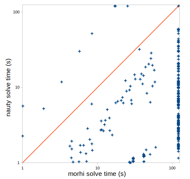
Figure 11. A comparison of behaviour of nauty and morphi on particular instances. Times are given in seconds

In the rest of this section, we provide the evaluation of the proof generation and certification, using our solver morphi (with the proving capabilities enabled), and our prototypical checker, also described in the previous section. We consider two different versions of morphi, implementing the two different proof generating strategies, explained in the previous section:

• morphi-d: the during-search strategy

• morphi-p: the post-search strategy

The instances used in this stage of evaluation are exactly those instances that our solver morphi without proof generating capabilities managed to solve in the time limit of 60 seconds (i.e. the instances selected in the previous stage of evaluation, 709 instances in total). Both versions of the solver morphi were run on all these 709 instances, this time without a time limit, with the proof generation enabled. In both cases, the generated proofs were verified using our prototypical checker.

The main result of the evaluation is that the proof verification was successful for all tested instances, i.e. for all generated proofs our checker confirmed their correctness.

For each instance we also measure several parameters that are important for estimating the impact of the proof generation and checking on the overall performance, as well as for comparing the two variants of the proof generating strategy. The solve time is the time spent in computing the canonical form. The prove time is the time spent in the proof generation. Notice that in case of morphi-d, we can only measure the sum of the solve time and the prove time, since the two phases are intermixed. The check time is the time spent in verifying the proof. We also measure the proof size.

Some interesting relations between the measured parameters on particular instances are depicted by scatter plots given in Figure 12, and corresponding minimal, maximal and average ratios are given in Table 3. We discuss these relations in more details in the following paragraphs.

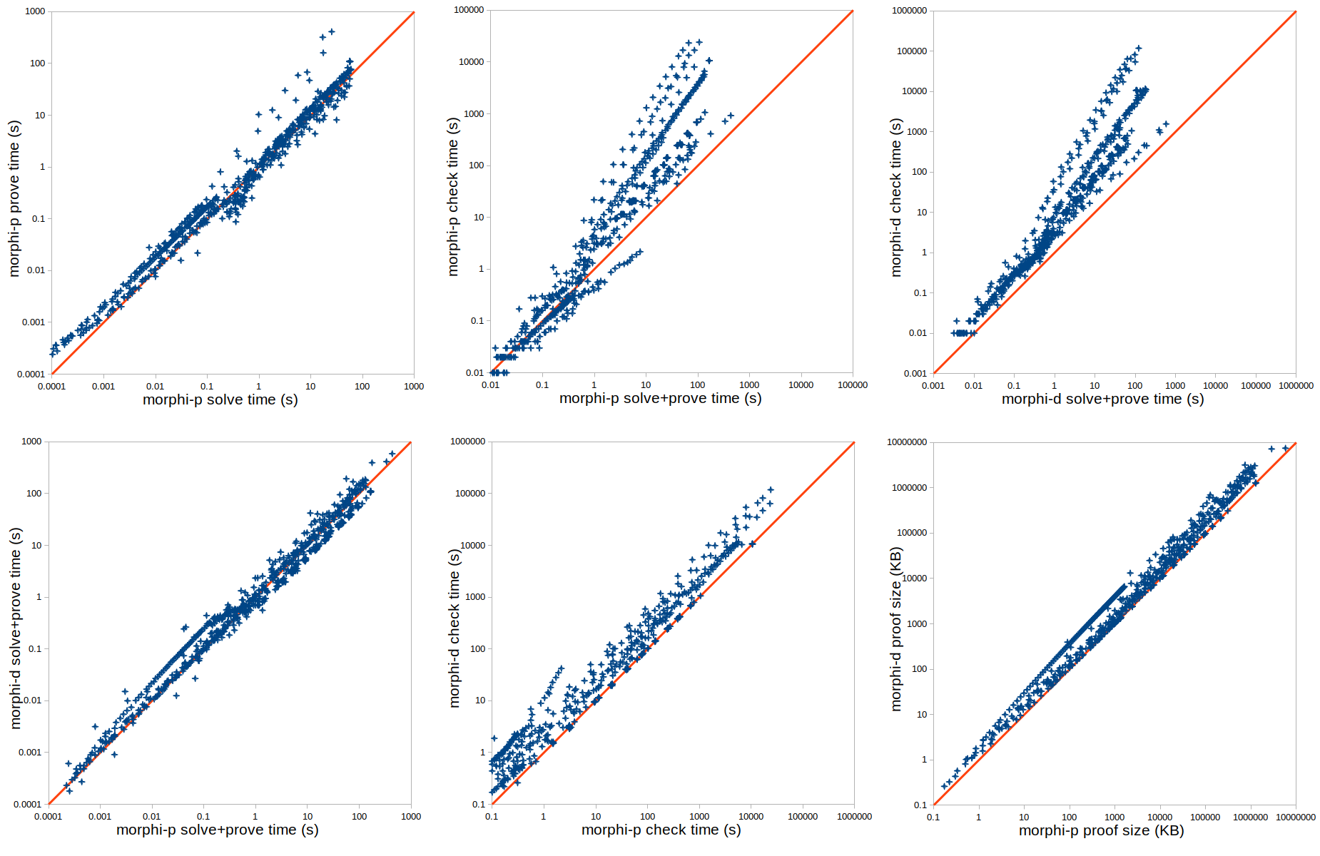
Figure 12. Behavior of morphi and the checker on particular instances. Times are given in seconds, and proof sizes are given in kilobytes

Ratio	Min	Max	Average
solve/prove (morphi-p)	0.053	4.090	0.886
(prove+solve)/check (morphi-p)	0.003	3.547	0.558
(prove+solve)/check (morphi-d)	0.001	1.009	0.219
morphi-p/morphi-d (solve+prove)	0.169	2.529	1.070
morphi-p/morphi-d (check)	0.048	1.192	0.555
morphi-p/morphi-d (proof size)	0.166	1.000	0.674

Table 3. Minimum, maximum and average ratios between the observed parameters on all tested instances

Solve time vs. prove time.

Top-left plot in Figure 12 shows the relation between the solve time and the prove time for morphi-p. The solve time was about 89% of the prove time on average, which means that the proof generation tends to take slightly more time than the search. In other words, the invocation of the algorithm with proof generation enabled on average takes over twice as much time as the canonical form search alone. This was somewhat expected, since the proof is generated by performing the search once more, using the information gathered during the first tree traversal.

Solve+prove time vs. check time.

Top-middle and top-right plots in Figure 12 show the relation between solve+prove time and check time, for morphi-p and morphi-d, respectively. From the plots it is clear that the proof verification tends to take significantly more time than the search and the proof generation together, and this is especially noticeable on “harder” instances. The average (solve+prove)/check ratio was 0.558 for morphi-p, with minimal ratio on all instances being 0.003. The phenomenon is even more prominent for morphi-d (0.219 average, 0.001 minimal). Such behavior can be explained by the fact that the checker is implemented with the simplicity of the code in mind (in order to make it more reliable), and not its efficiency. Most of the conditions in the rule applications are checked by brute force. On the other hand, the search algorithm’s implementation is heavily optimized for best performance.

Comparing the proof generating strategies.

Bottom-left, bottom-middle and bottom-right plots in Figure 12 compare the morphi-p and morphi-d with respect to the solve+prove times, check times and proof sizes, respectively. The solve+prove times were similar on average (morphi-d being slightly faster, with the average solve+prove time equal to 17.7s, while for morphi-p it was 18.9s). Most of the points on the bottom-left plot are very close to the diagonal, almost evenly distributed on both sides of it. The average solve+prove time ratio was very close to 1 (1.07). This suggests that, when the time consumed by the algorithm is concerned, it does not matter which proof generation strategy is employed. On the other hand, the size of a morphi-p proof was about 67% of the size of the corresponding morphi-d proof on average, and a morphi-p proof was never greater than the corresponding morphi-d proof. Finally, the check time for proofs generated by morphi-p was about 55.5% of the check time for proofs generated by morphi-d on average. This means that the proof checking will be more efficient if we employ the post-search proof generation strategy. One of the main reasons for that is significantly smaller average proof size, but this might not be the only reason. Namely, the check time does not depend only on the proof size, but also on the structure of the proof, since some rules are harder to check than others. The most expensive check is required by Equitable, InvariantsEqual, PruneInvariant and PruneLeaf rules, since it includes time consuming operations such as verifying the equitability of the coloring, calculating the hash function for colored graphs, or comparing the graphs. These operations tend to be more expensive as we move towards the leaves of the search tree, i.e. as the colorings become closer to discrete. In post-search proof generating strategy, the prunings tend to happen higher in the search tree during the second tree traversal (when the proof is actually generated), lowering the proportion of these expensive rules in the proof.

5.4. False proofs

It is important to stress that the checker does not only accept correct proofs, but that it indeed rejects false proofs as well. Some issues with the solver were found and resolved during development as a consequence of false proofs that had been rejected by the checker. For example, there were issues with the invariant calculation and the coloring refinement that led to incorrect canonical forms and proofs being produced for some instances. There was also an issue that caused emission of false facts into the proof in some occasions, specifically during the traversal of a pruned subtree in search for automorphisms. As a part of further testing, several artificial bugs were introduced into the solver which were successfully caught by the checker.

6. Related work

Certifying algorithms in general.

There are many applications in the industry or science where a user may benefit of having an algorithm which produces certificates that can confirm the correctness of its outputs. McConnell et al. [MMNS11] go one step further, suggesting that every algorithm should be certifying, i.e. be able to produce certificates. They establish a general theoretical framework for studying and developing certifying algorithms, and provide a number of examples of practical algorithms that could be extended to produce certificates. The authors stress two important properties of a certifying algorithm that must be fulfilled: simplicity, which means that it is easy to prove that the (correct) certificates really certify the correctness of the obtained outputs, and checkability, which means that it is easy to check the correctness of a certificate. In both cases, the property of being easy is not strictly defined.

In case of simplicity, it is expected that the fact that a certificate really proves the correctness of the corresponding output should be obvious and easily understandable. This may be considered as a potential drawback of our approach, since the soundness of our proof system is not obvious and requires a non-trivial proof. However, we did our best to provide an as precise as possible soundness proof in the appendix of this paper, with hope that it is convincing enough to the reader (we also prove the completeness, i.e. the existence of a certificate for each input, for which McConnell et al. [MMNS11] do not insist to be simple to prove). We have also formalized the soundness proof within Isabelle/HOL theorem prover, and we believe that the existence of a formal soundness proof is a good substitution for the simplicity property stressed by the authors.

When checkability is concerned, the authors suggest that an algorithm for certificate checking should either have a simple logical structure, such that its correctness can be easily established, or it should be formally verified [MMNS11]. We believe that our checker indeed has a simple logical structure, since its most complicated parts such as calculating $\operatorname{split}(G,\pi,i)$ function are implemented using a brute force, without any sofisticated data structures or programming techniques. Moreover, we have already argued (see Subsection 5.2) that its implementation is much simpler than the implementation of the canonical labelling algorithm itself, and can be more easily verified. In fact, we have already provided and formally verified an abstract proof checker specification in Isabelle/HOL. The remaining step is to refine this abstract specification into an efficient executable code, which we plan to do in the future.

McConnell et al. [MMNS11] also suggest that the complexity of a certificate checking algorithm should preferably be linear with respect to the size of its input, and its input is composed of an input/output pair of the certifying algorithm, and of the corresponding certificate. In our case, each rule from the certificate is read and checked exactly once, but checking of some rules may require traversing the graph’s adjacency matrix, so the complexity is not exactly linear. However, since the size of the proof is usually much greater than the size of the graph, the complexity may be considered to be almost linear.

Certifying algorithms in SAT solving.

Certificate checking has been successfully used, for example, in certifying unsatisfiability results given by SAT or SMT solvers [WHJ14, HKM16, Lam20], and this enabled application of external SAT and SMT solvers from within interactive theorem provers [Web06, Böh12, BBP11].

The proof system used in the case of SAT solvers is very simple and is based on the resolution. While early approaches considered simple resolution proofs [ZM03] which were very easy to check, but much harder to produce, modern approaches are mostly based on so-called reversed unit-propagation (RUP) proofs [Gel08], which are easy to generate, but harder to check. While this fact violates the checkability property to some extent, it is widely adopted by the SAT solving community, and proof formats such as DRAT [WHJ14] became an industry standard in the field. Our proof system has a similar trait, since we retained some complex computations within the checker, in order to make our proofs smaller and easier to generate. As with RUP proofs, we consider this as a good tradeoff.

Certifying pseudo-boolean reasoning.

The SAT problem is naturally generalized to the pseudo-boolean (PB) satisfiability problem [RM21], where it is also useful to have certifying capabilities. Recently, a simple but expressive proof format for proving the PB unsatisfiability was proposed by Elffers et al. [EGM⁺20], based on cutting planes [CCT87]. That proof format was then employed for expressing unsatisfiability proofs for different combinatorial search and optimization problems, such as constraint satisfaction problems involving the alldifferent constraint [EGM⁺20], the subgraph isomorphism problem [GMN21], and the maximum clique and the maximum common subgraph problem [GMM⁺20]. The main idea is to express some combinatorial problem $P$ as a pseudo-boolean problem $PB(P)$, and then to express the reasonings of a dedicated solver for $P$ in terms of PB constraints implied by the constraints of $PB(P)$ (such PB constraints are exported by the dedicated solver during the solving process). The obtained PB proof is then checked by an independent checker which relies on a small number of simple rules (such as addition of two PB constraints or multiplying/dividing a PB constraint with a positive constant), as well as on generalized RUP derivations [EGM⁺20]. The authors advocate the generality of their approach, enabling it to express the reasoning employed in solving many different combinatorial problems, using a simple and general language which does not know anything about the concepts and specific semantics of considered problems.

In contrast, our proof system is tied to a particular problem – the problem of constructing canonical graph labellings, and a particular class of algorithms – those that could be instantiated from the McKay/Piperno scheme [MP14]. Citing McKay, the canonical forms returned by the algorithm considered in this paper are “designed to be efficiently computed, rather than easily described” [McK98]. Since the canonical labelling specification is given in terms of the algorithm, it seems that certification must also be tied to it. This is the main reason that led to our decision to develop an algorithm-specific proof format which is powerful enough to capture all the reasonings that appear in the context of this particular class of labelling algorithms.

The question remains whether the canonical labelling problem, like some other graph problems previously mentioned, may be encoded in terms of PB constraints in a way simple enough to be trusted (as noted by Gocht et al. [GMM⁺20], an encoding should be simple – since it is not formally verified, any errors in the encoding may lead to “proving the wrong thing”). Moreover, the encoding should permit expressing the operations made by the canonical labelling algorithm in terms of PB constraints implied by the encoding. Up to the authors’ knowledge, it is not obvious whether such encoding exists. The main issue that we see in such an approach is that the canonical form of the graph, as defined by McKay and Piperno [MP14], is not simple to describe in advance using PB constraints, since it is defined implicitly by the canonical labelling algorithm itself. For instance, one should capture the notion of “coarsest equitable coloring finer than a given coloring $\pi$”, which is especially hard if we know that such a coloring is not unique, so we must fix one particular ordering of the cells (and that ordering must be also captured using the PB language). The similar case is with describing hash functions used in calculating node invariants.

7. Conclusions and further work

We have formulated a proof-system for certifying that a graph is a canonical form of another graph, which is a key step in verifying graph isomorphism. The proof system is based on the state-of-the-art scheme of McKay and Piperno and we proved its soundness and completeness. Our algorithm implementation produces proofs that can be checked by an independent proof checker. The implementation of the proof checker is much simpler than the implementation of the core algorithm, so it is easier to trust.

One of the main problems with our approach is that our proof format is very closely related to the canonical labelling algorithm itself. Therefore, it is very difficult to use our proof format and proof checker for different approaches to isomorphism checking. On the other hand, the McKay/Piperno scheme is broad enough to cover several state-of-the-art algorithms, and we believe that our proofs and checkers can be easily adapted to certify all these algorithms. Our prototype implementation morphi is slower compared to state-of-the-art implementations such as nauty, but still comparable on many instances. We plan to make further optimizations to morphi. We are also considering adapting nauty’s source-code to emit proofs in our format, which is not trivial, as nauty has been developed for more than 30 years and is a very complex and highly optimized software system.

The main direction of our further work is to go one step further and fully integrate isomorphism checking into an interactive theorem prover. We have already taken important steps in this direction: we have formally defined the McKay and Piperno’s abstract scheme in Isabelle/HOL and formally proved its correctness (Theorem 1), we have shown that our concrete functions $\bar{R}$, $\bar{T}$, and $\bar{\phi}$ satisfy the McKay/Piperno axioms, and we have formalized the rules of our proof system and formally proved its soundness. We have also provided and formally verified an abstract proof checker specification in Isabelle/HOL. In our further work it remains to refine our abstract proof checker specification into efficient executable code, which we plan to do using Imperative Refinement Framework [Lam16].

Another direction of our further work is to examine the possibilities of reducing the complexity of our proof system. Currently, our system operates with 9 different types of facts and has 18 different rules. Compared to some other well-known proof systems, such as those used in SAT or PB solving, which rely on few very simple rules, our system may be much harder to understand and trust, and proof checking becomes a non-trivial task. We tried to fill this gap by providing a formal proof of the soundness of our system in Isabelle/HOL, together with a (verified) abstract specification of our proof checker. However, it would be beneficial to develop a simpler proof system or to find a way to reduce our system to some existing proof system which is well understood and trusted (such as those mentioned above). We are currently not aware if this is possible in case of graph canonical labelling algorithms based on McKay and Piperno’s abstract scheme, so this remains a great challenge that may be interesting to tackle in further work.

Appendix A Proofs of lemmas and theorems

Theorem (1).

If $R$, $T$, and $\phi$ satisfy all axioms, then for the function $C$ determined by $R$, $T$ and $\phi$ it holds that two colored graphs $(G,\pi_{0})$ and $(G^{\prime},\pi_{0}^{\prime})$ are isomorphic if and only if $C(G,\pi_{0})=C(G^{\prime},\pi_{0}^{\prime})$.

Proof A.1.

Assume that $(G,\pi_{0})$ and $(G^{\prime},\pi_{0}^{\prime})$ are isomorphic. Then exists a permutation $\sigma\in S_{n}$ such that $(G^{\prime},\pi_{0}^{\prime})=(G^{\sigma},\pi_{0}^{\sigma})$. Since the functions $R$ and $T$ are label-invariant, it is easy to show that $\mathcal{T}(G^{\sigma},\pi_{0}^{\sigma},\nu^{\sigma})=\mathcal{T}(G,\pi_{0},\nu)^{\sigma}$. Moreover, since $\phi$ is also label-invariant, if $\nu$ is a leaf from $\mathcal{T}(G,\pi_{0})$, and $\nu^{\sigma}$ is the corresponding leaf from $\mathcal{T}(G^{\sigma},\pi_{0}^{\sigma})$, then $\phi(G,\pi_{0},\nu)=\phi(G^{\sigma},\pi_{0}^{\sigma},\nu^{\sigma})$, so the leaves that correspond to each other with respect to $\sigma$ have equal node invariants. Therefore, the sets of maximal leaves of the two trees correspond to each other, with respect to $\sigma$. Furthermore, if $R(G,\pi_{0},\nu)=\pi$, for some leaf $\nu\in\mathcal{T}(G,\pi_{0})$, then $R(G^{\sigma},\pi_{0}^{\sigma},\nu^{\sigma})=R(G,\pi_{0},\nu)^{\sigma}=\pi^{\sigma}=\sigma^{-1}\pi$, and we have $(G^{\sigma})^{\pi^{\sigma}}=(G^{\sigma})^{\sigma^{-1}\pi}=G^{\sigma\sigma^{-1}\pi}=G^{\pi}$, so the graphs that correspond to the leafs $\nu\in\mathcal{T}(G,\pi_{0})$ and $\nu^{\sigma}\in\mathcal{T}(G^{\sigma},\pi_{0}^{\sigma})$ are identical. Therefore, the maximal graphs that correspond to the maximal leaves in both trees are also identical, so $C(G,\pi_{0})=C(G^{\sigma},\pi_{0}^{\sigma})=C(G^{\prime},\pi_{0}^{\prime})$ (although the canonical leaves of the trees $\mathcal{T}(G,\pi_{0})$ and $\mathcal{T}(G^{\sigma},\pi_{0}^{\sigma})$ do not have to correspond to each other with respect to $\sigma$).

Conversely, assume that $C(G,\pi_{0})=C(G^{\prime},\pi_{0}^{\prime})$. Since $C(G,\pi_{0})$ is a graph assigned to some leaf of $\mathcal{T}(G,\pi_{0})$, then there exists a permutation $\sigma\in S_{n}$ such that $C(G,\pi_{0})=(G^{\sigma},\pi_{0}^{\sigma})$. Similarly, there exists a permutation $\sigma^{\prime}\in S_{n}$ such that $C(G^{\prime},\pi_{0}^{\prime})=(G^{\prime\sigma^{\prime}},\pi_{0}^{\prime\sigma^{\prime}})$. Since $(G^{\sigma},\pi_{0}^{\sigma})=(G^{\prime\sigma^{\prime}},\pi_{0}^{\prime\sigma^{\prime}})$, we have $(G^{\prime},\pi_{0}^{\prime})=(G^{\sigma},\pi_{0}^{\sigma})^{\sigma^{\prime-1}}=(G,\pi_{0})^{\sigma\sigma^{\prime-1}}$, so $(G,\pi_{0})$ and $(G^{\prime},\pi_{0}^{\prime})$ are isomorphic.

Lemma (2).

For each $\sigma\in S_{n}$, $\mathtt{make\_equitable}(G^{\sigma},\pi^{\sigma},\alpha^{\sigma})=\mathtt{make\_equitable}(G,\pi,\alpha)^{\sigma}$.

Proof A.2.

Let $\pi^{\prime}$ and $\pi_{\sigma}^{\prime}$ be the current colorings in invocations $\mathtt{make\_equitable}(G,\pi,\alpha)$ and $\mathtt{make\_equitable}(G^{\sigma},\pi^{\sigma},\alpha^{\sigma})$ respectively. Similarly, let $\alpha$ and $\alpha_{\sigma}$ be the current lists of splitting cells in the two invocations. We prove by induction that, for each $k$, after $k$ iterations of the $while$ loop in both invocations it holds that $\pi_{\sigma}^{\prime}={\pi^{\prime}}^{\sigma}$ and $\alpha_{\sigma}=\alpha^{\sigma}$. The statement holds initially, for $k=0$, since $\pi^{\prime}=\pi$, $\pi_{\sigma}^{\prime}=\pi^{\sigma}$ and $\alpha_{\sigma}=\alpha^{\sigma}$. Assume that statement holds for some $k$. First notice that $\pi^{\prime}$ is a discrete coloring after $k$ iterations if and only if $\pi_{\sigma}^{\prime}$ is discrete, since $\pi_{\sigma}^{\prime}={\pi^{\prime}}^{\sigma}$, by induction hypothesis. Similarly, $\alpha$ is empty if and only if $\alpha_{\sigma}$ is empty, since $\alpha_{\sigma}=\alpha^{\sigma}$. Therefore, either both invocations enter the next iteration of the $while$ loop, or both finish the execution of the algorithm after $k$-th iteration, returning $\pi^{\prime}$ and $\pi^{\prime\sigma}$, respectively. In the first case, if $W$ is the first cell of $\pi^{\prime}$ that belongs to $\alpha$, then $W^{\sigma}$ is the first cell of $\pi_{\sigma}^{\prime}$ belonging to $\alpha_{\sigma}$, since $\pi_{\sigma}^{\prime}={\pi^{\prime}}^{\sigma}$ and $\alpha_{\sigma}=\alpha^{\sigma}$ by induction hypothesis, and the relabelling does not change the order of the cells. Moreover, if a cell $X\in\pi^{\prime}$ is partitioned into $X_{1},X_{2},\ldots,X_{k}$, then the corresponding cell $X^{\sigma}\in{\pi^{\prime}}^{\sigma}$ is partitioned into $X_{1}^{\sigma},X_{2}^{\sigma},\ldots,X_{k}^{\sigma}$, with $|X_{i}^{\sigma}|=|X_{i}|$, since the partitioning (and the order of partitions) depends only on the number of adjacent vertices from $W$, which is not affected by relabelling. This implies that the statement also holds after $k+1$ iterations of the $while$ loop. This proves the lemma, since both invocations finish after equal numbers of iterations.

Lemma (3).

If $\pi^{\prime}=\mathtt{make\_equitable}(G,\pi,\alpha)$, then $\pi^{\prime}\preceq\pi$.

Proof A.3.

The lemma follows from the fact that the only type of transformation that is applied to the given coloring $\pi$ by the procedure $\mathtt{make\_equitable}$ is splitting of its cells, which always produces a finer coloring.

Lemma (4).

If $\pi=\bar{R}(G,\pi_{0},\nu)$, then:

1. $\pi\preceq\pi_{0}$

2. $\pi$ individualizes vertices from $\nu$

3. for each $\sigma\in S_{n}$, $\bar{R}(G^{\sigma},\pi_{0}^{\sigma},\nu^{\sigma})=\bar{R}(G,\pi_{0},\nu)^{\sigma}$

Proof A.4.

The lemma will be proved by induction on $k=|\nu|$. For $k=0$, we have $\nu=[\ ]$, the statement follows from Lemma 2 and Lemma 3. Assume that the statement holds for some $k$ and let $\nu=[\nu^{\prime},v]$, where $|\nu^{\prime}|=k$. Notice that $\bar{R}(G,\pi_{0},[\nu^{\prime},v])$ first invokes $\bar{R}(G,\pi_{0},\nu^{\prime})$. The statement holds for the coloring $\pi^{\prime}$ returned by the recursive call, by induction hypothesis. The procedure additionally individualizes the vertex $v$, obtaining the coloring $\pi^{\prime\prime}$, and then calls $\mathtt{make\_equitable}(G,\pi^{\prime\prime},\alpha)$, where $\alpha=\{\{v\}\}$. Let $\pi$ be the coloring returned by this call. Since $\pi^{\prime\prime}$ is obtained from $\pi^{\prime}$ by individualization of the vertex $v$, it holds $\pi^{\prime\prime}\preceq\pi^{\prime}$. By Lemma 3, we have $\pi\preceq\pi^{\prime\prime}$, and by induction hypothesis, it holds $\pi^{\prime}\preceq\pi_{0}$. Therefore, $\pi\preceq\pi_{0}$, by transitivity of $\preceq$. Since $\pi^{\prime}$ individualizes the vertices from $\nu^{\prime}$ (by induction hypothesis), then coloring $\pi$ individualizes the vertices from $\nu$ (since $\pi\preceq\pi^{\prime\prime}\preceq\pi^{\prime}$ and the vertex $v$ is also individualized in $\pi^{\prime\prime}$). Finally, since $\bar{R}(G^{\sigma},\pi_{0}^{\sigma},\nu^{\prime\sigma})=\pi^{\prime\sigma}$ (by induction hypothesis), and since the cell containing $v^{\sigma}$ in $\pi^{\prime\sigma}$ is $W^{\sigma}$, where $W$ is the cell containing $v$ in $\pi^{\prime}$, it follows that the coloring obtained from $\pi^{\prime\sigma}$ after the individualization of $v^{\sigma}$ will be equal to $\pi^{\prime\prime\sigma}$, where $\pi^{\prime\prime}$ is obtained from $\pi^{\prime}$ by individualization of $v$. Furthermore, $\{\{v^{\sigma}\}\}=\alpha^{\sigma}$, so we have $\mathtt{make\_equitable}(G^{\sigma},\pi^{\prime\prime\sigma},\alpha^{\sigma})=\mathtt{make\_equitable}(G,\pi^{\prime\prime},\alpha)^{\sigma}$, by Lemma 2.

Lemma (5).

Let $W$ be the cell of $\pi^{\prime}$ that is chosen as a splitting cell in some arbitrary iteration of the while loop of the procedure $\mathtt{make\_equitable}(G,\pi,\alpha)$. Let $W^{\prime}$ be any cell of $\pi^{\prime}$ that precedes $W$ in $\pi^{\prime}$ (that is, it corresponds to a smaller color). Then $W^{\prime}$ does not cause any splitting, i.e., for any two vertices of a same color in $\pi^{\prime}$ the numbers of their adjacent vertices from $W^{\prime}$ are equal.

Proof A.5.

To simplify terminology, we call the cells $W^{\prime}$ satisfying the condition stated in the last sentence of the lemma neutral. More precisely, we say that a set $X$ of vertices from a graph $G$ is neutral with respect to a coloring $\pi$, if for each cell $W$ of $\pi$ and for each two vertices $v_{1}$ and $v_{2}$ from $W$ the numbers of vertices from $X$ adjacent to $v_{1}$ and $v_{2}$ are equal. In that terminology, the lemma claims that any cell $W^{\prime}$ of $\pi^{\prime}$ preceding $W$ is neutral with respect to $\pi^{\prime}$.

Note that if some set $X$ is neutral with respect to a coloring $\pi$, then it is also neutral with respect to any coloring $\overline{\pi}$ finer than $\pi$.

Furthermore, we say that a cell $X$ of $\pi$ is conditionally neutral with respect to $\pi$ if for each coloring $\overline{\pi}$ finer than or equal to $\pi$ if all the cells that precede $X$ in $\pi$ are neutral with respect to $\overline{\pi}$, then $X$ is also neutral with respect to $\overline{\pi}$. Note that if a cell $X$ is neutral with respect to $\pi$, it is also conditionally neutral with respect to $\pi$.

We first prove the following two propositions.

Proposition 18.

Let $X$ be a cell of a coloring $\pi$ which is conditionally neutral with respect to $\pi$, and let $\overline{\pi}$ be any coloring finer than $\pi$ (i.e. obtained by partitioning some of its cells). Let $X_{1},\ldots,X_{k}$ (in that order) be partitions of $\overline{\pi}$ obtained by partitioning the cell $X$ of $\pi$. Then $X_{k}$ is conditionally neutral with respect to $\overline{\pi}$.

To prove this proposition, first notice that $\overline{\pi}\preceq\pi$. Let $\hat{\pi}$ be any coloring finer than $\overline{\pi}$ such that all the cells of $\overline{\pi}$ that precede $X_{k}$ are neutral with respect to $\hat{\pi}$. We must prove that $X_{k}$ is also neutral with respect to $\hat{\pi}$. Let $Y$ be any cell of $\pi$ that precedes $X$ in $\pi$, and let $Y_{1},\ldots,Y_{m}$ be the cells of $\overline{\pi}$ obtained by partitioning the cell $Y$. Since $Y_{1},\ldots,Y_{m}$ precede $X_{k}$ in $\overline{\pi}$, these cells are neutral with respect to $\hat{\pi}$ by assumption. Then it is easy to argue that $Y$ is also neutral with respect to $\hat{\pi}$ – the number of adjacent vertices from $Y$ to each vertex $v$ is obtained by summing the numbers of adjacent vertices from $Y_{1},\ldots,Y_{m}$, so for any two same-colored vertices (with respect to $\hat{\pi}$) such sums must be equal. Now, since $\hat{\pi}\preceq\overline{\pi}\preceq\pi$, and all the cells that precede $X$ in $\pi$ are neutral with respect to $\hat{\pi}$, then $X$ must be also neutral with respect to $\hat{\pi}$ (because it is conditionally neutral with respect to $\pi$ by assumption). Furthermore, since the cells $X_{1},\ldots,X_{k-1}$ are also neutral with respect to $\hat{\pi}$ by assumption (because they precede $X_{k}$ in $\overline{\pi}$), then the cell $X_{k}$ is also neutral with respect to $\hat{\pi}$ (since $X$ is neutral with respect to $\hat{\pi}$, and the number of adjacent vertices from $X_{k}$ to any vertex $v$ can be obtained by subtracting the sum of the numbers of its adjacent vertices from $X_{1},\ldots,X_{k-1}$ from the number of its adjacent vertices from $X$. Again, for the same-colored vertices with respect to $\hat{\pi}$, such numbers must be equal). Now it follows that $X_{k}$ is conditionally neutral with respect to $\overline{\pi}$, as stated by the proposition.

Proposition 19.

Let $X_{1},\ldots,X_{k}$ be the first $k$ cells of a coloring $\pi$. If $X_{1},\ldots,X_{k}$ are conditionally neutral with respect to $\pi$, then they are also neutral with respect to $\pi$.

This proposition may be proven by induction on the cell index. For the cell $X_{1}$ the statement trivially holds, since there are no cells that precede it in $\pi$, so it must be neutral with respect to any coloring finer than or equal to $\pi$, including $\pi$ itself. Assume the statement holds for $X_{1},\ldots,X_{i-1}$, and let us prove that it holds for $X_{i}$ ($i\leq k$). Since $X_{i}$ is conditionally neutral with respect to $\pi$ it must be neutral with respect to any coloring finer than or equal to $\pi$ such that all the cells $X_{1},\ldots,X_{i-1}$ are also neutral with respect to it. By induction hypothesis, $X_{1},\ldots,X_{i-1}$ are neutral with respect to $\pi$, and since $\pi\preceq\pi$, the cell $X_{i}$ must also be neutral with respect to $\pi$.

Proposition 20.

In the procedure $\mathtt{make\_equitable}(G,\pi,\alpha)$, at the beginning of each iteration of the while loop, any cell $X$ of $\pi^{\prime}$ that is not present in $\alpha$ is conditionally neutral with respect to $\pi^{\prime}$.

This claim can be proven by induction on the number of iterations. In the base case, before the first iteration of the loop (when $\pi^{\prime}=\pi$), we have two cases to consider. The first case is when the procedure is called initially, with $\alpha$ containing all the cells of $\pi$. In that case, the statement trivially holds, since there are no cells of $\pi^{\prime}$ that are not in $\alpha$. The second case is when the procedure is invoked with only one singleton cell $\{v\}$ in $\alpha$, where $v$ is the last individualized vertex. Let $\overline{\pi}$ be the coloring obtained from $\pi$ by partitioning the cell $V$ containing $v$ into $\{v\}$ and $V\setminus\{v\}$ (in that order). Since the coloring $\pi$ was already equitable before individualization of $v$, all the cells of $\pi$ (including $V$) are neutral with respect to $\pi$. Therefore, all the cells of $\pi$ distinct from $V$ (which are also the cells of $\overline{\pi}$ and are not in $\alpha$) are neutral with respect to $\overline{\pi}$, and therefore, conditionally neutral with respect to $\overline{\pi}$. On the other hand, since $V$ is neutral with respect to $\pi$, it is also conditionally neutral with respect to $\pi$. By 18, the cell $V\setminus\{v\}$ is conditionally neutral with respect to $\overline{\pi}$. Thus, all cells of $\overline{\pi}$ not in $\alpha$ are conditionally neutral with respect to $\overline{\pi}$.

In order to prove the induction step, let us assume that the statement holds before $k$-th iteration. Let $W\in\alpha$ be the next splitting cell chosen by the algorithm, and let $\overline{\pi}$ be the coloring obtained from $\pi^{\prime}$ by partitioning its cells with respect to $W$. At the end of $k$-th iteration, the following cells of $\overline{\pi}$ will not be in $\alpha$:

• since $W$ is removed from $\alpha$ at the beginning of $k$-th iteration, if $W$ is partitioned to $W_{1},\ldots,W_{k}$ (in that order), then $W_{k}$ will not be in $\alpha$. Since $\overline{\pi}$ is obtained from $\pi^{\prime}$ by partitioning its cells with respect to $W$, then $W$ is neutral with respect to $\overline{\pi}$, and also with respect to any coloring $\hat{\pi}$ finer than $\overline{\pi}$. Therefore, if $W_{1},\ldots,W_{k-1}$ are neutral with respect to $\hat{\pi}$, the cell $W_{k}$ will be also neutral with respect to $\hat{\pi}$. By definition, it follows that $W_{k}$ is conditionally neutral with respect to $\overline{\pi}$.

• for any cell $X$ of $\pi^{\prime}$ that was not in $\alpha$ at the beginning of $k$-th iteration, if $X$ is partitioned to $X_{1},\ldots,X_{k}$ (in that order), $X_{k}$ will not be in $\alpha$. By induction hypothesis, $X$ is conditionally neutral with respect to $\pi^{\prime}$, so by 18, $X_{k}$ is conditionally neutral with respect to $\overline{\pi}$.

Therefore, all the cells of $\overline{\pi}$ not in $\alpha$ at the end of $k$-th iteration are conditionally neutral with respect to $\overline{\pi}$. By proving the induction step, we have proven the proposition.

Now let us return to the proof of the main lemma. It easily follows from the previous propositions, since all the cells preceding $W$ in $\pi^{\prime}$ are not in $\alpha$, thus conditionally neutral with respect to $\pi^{\prime}$ by 20, and therefore neutral with respect to $\pi^{\prime}$ by 19.

Lemma (6).

For each $\sigma\in S_{n}$ it holds $\bar{T}(G^{\sigma},\pi_{0}^{\sigma},\nu^{\sigma})=\bar{T}(G,\pi_{0},\nu)^{\sigma}$.

Proof A.6.

The lemma holds since, according to Lemma 4, $\bar{R}(G^{\sigma},\pi_{0}^{\sigma},\nu^{\sigma})=\bar{R}(G,\pi_{0},\nu)^{\sigma}$, so their first non-singleton cells also correspond to each other, with respect to $\sigma$.

Lemma (7).

The following properties of the function $\bar{\phi}$ hold:

1. If $|\nu^{\prime}|=|\nu^{\prime\prime}|$ and $\bar{\phi}(G,\pi_{0},\nu^{\prime})<\bar{\phi}(G,\pi_{0},\nu^{\prime\prime})$, then $\bar{\phi}(G,\pi_{0},[\nu^{\prime},w_{1}])<\bar{\phi}(G,\pi_{0},[\nu^{\prime\prime},w_{2}])$, for each $w_{1}\in T(G,\pi_{0},\nu^{\prime})$, $w_{2}\in T(G,\pi_{0},\nu^{\prime\prime})$

2. For each $\nu$ and nonempty $\nu^{\prime}$ such that $[\nu,\nu^{\prime}]$ is a tree node, it holds that $\bar{\phi}(G,\pi_{0},\nu)<\bar{\phi}(G,\pi_{0},[\nu,\nu^{\prime}])$.

3. $\bar{\phi}(G^{\sigma},\pi_{0}^{\sigma},\nu^{\sigma})=\bar{\phi}(G,\pi_{0},\nu)$ for each node $\nu$ and for each permutation $\sigma\in S_{n}$

Proof A.7.

The first two properties hold trivially, since the node invariants are compared lexicographically. For the third property, recall that we assumed that the function $\operatorname{f}_{hash}$ is label invariant, i.e. $\operatorname{f}_{hash}(G^{\sigma},\pi^{\sigma})=\operatorname{f}_{hash}(G,\pi)$. By Lemma 4, the equality:

$$\operatorname{f}_{hash}(G^{\sigma},\bar{R}(G^{\sigma},\pi_{0}^{\sigma},[\nu]_{i}^{\sigma}))=\operatorname{f}_{hash}(G^{\sigma},\bar{R}(G,\pi_{0},[\nu]_{i})^{\sigma})=\operatorname{f}_{hash}(G,\bar{R}(G,\pi_{0},[\nu]_{i}))$$

holds for each $i\leq|\nu|$. Therefore, we have $\bar{\phi}(G^{\sigma},\pi_{0}^{\sigma},\nu^{\sigma})=\bar{\phi}(G,\pi_{0},\nu)$.

Lemma (8).

For each of the rules in our proof system, if all its premises are valid facts for the graph $(G,\pi_{0})$, and all additional conditions required by the rule are fulfilled, then the facts that are derived by the rule are also valid facts for the graph $(G,\pi_{0})$.

Proof A.8.

We prove the statement of the lemma for each of the rules of our proof system. For the rule ColoringAxiom, first notice that the fact $\pi_{0}\xrightarrow{eq}\bar{R}(G,\pi_{0},[\ ])$ is obviously valid, since $\bar{R}(G,\pi_{0},[\ ])$ is obtained by invoking the procedure $\mathtt{make\_equitable}(G,\pi_{0},\alpha)$, where $\alpha$ is the set of all cells of $\pi_{0}$ (Algorithm 2). Also, the empty sequence is the root node of any search tree, so the fact $[\ ]\in\mathcal{T}(G,\pi_{0})$ is also valid.

For the rule Individualize, from the first premise we have that the coloring assigned to the node $\nu$ is equal to $\pi$. From the second premise, the sequence $[\nu,v]$ is also a node of the search tree $\mathcal{T}(G,\pi_{0})$. Since the coloring assigned to the node $[\nu,v]$ is constructed from $\pi$ by individualizing the vertex $v$ and then making the coloring equitable (Algorithm 2) the fact $\operatorname{individualize}(\pi,v)\xrightarrow{eq}\bar{R}(G,\pi_{0},[\nu,v])$ is also valid.

For the rule SplitColoring, from the premise we have that the coloring assigned to the node $\nu$ is obtained by invoking the procedure $\mathtt{make\_equitable}$ for $\pi$. A consequence of Lemma 5 is that the coloring obtained after the first iteration of the while loop in the procedure $\mathtt{make\_equitable}$ (Algorithm 1) will be the coloring $split(G,\pi,i)$, where $i=min\{j\ |\ split(G,\pi,j)\prec\pi\}$ (and the rule assumes that such $i$ exists). Therefore, the rest of the iterations of the while loop will start with the coloring $split(G,\pi,i)$ and produce the coloring $\bar{R}(G,\pi_{0},\nu)$ at the end of the loop. It is easy to see that the same result would be obtained if $\mathtt{make\_equitable}$ was invoked for the coloring $split(G,\pi,i)$, that is, we have $split(G,\pi,i)\xrightarrow{eq}\bar{R}(G,\pi_{0},\nu)$.

For the rule Equitable, the premise tells us that the coloring assigned to the node $\nu$ is obtained from $\pi$ by invoking the procedure $\mathtt{make\_equitable}$. Since the rule assumes that there are no cells for which $\operatorname{split}(G,\pi,i)\prec\pi$, the coloring $\pi$ is equitable, so the application of the procedure $\mathtt{make\_equitable}$ on $\pi$ produces $\pi$ itself. This means that $\bar{R}(G,\pi_{0},\nu)=\pi$.

For the rule TargetCell, its premise is the fact $\bar{R}(G,\pi_{0},\nu)=\pi$, which claims that $\pi$ is the coloring assigned to the node $\nu$. Since the target cell is always the first non-singleton cell of the coloring assigned to a node (and the rule assumes that such a cell exists for the coloring $\pi$), the first fact the rule derives is valid. Furthermore, the sequences of the form $[\nu,v]$, where $v$ belongs to the target cell corresponding to $\nu$ are also the nodes of the tree, so the remaining facts derived by the rule are also valid.

For the rule InvariantAxiom, the fact $\bar{\phi}(G,\pi_{0},[\ ])=\bar{\phi}(G\pi_{0},[\ ])$ is obviously true, by reflexivity.

For the rule InvariantsEqual, if the invariants are equal for the parent nodes of the two given nodes $\nu_{1}$ and $\nu_{2}$ (which is one of the premises of the rule), and $\operatorname{f}_{hash}$ function takes equal values on $(G,\pi_{1})$ and $(G,\pi_{2})$, where $\pi_{1}$ and $\pi_{2}$ are the colorings corresponding to $\nu_{1}$ and $\nu_{2}$ respectively, then the node invariants are also equal for $\nu_{1}$ and $\nu_{2}$.

The correctness of the rule InvariantsEqualSym follows from the symmetry of the equality.

For the rule OrbitsAxiom, the fact of the form $\{v\}\vartriangleleft\operatorname{orbits}(G,\pi_{0},\nu)$ derived by the rule is always valid, provided that $v$ is a vertex of $G$ (which is assumed by the rule).

For the rule MergeOrbits, let $\sigma\in Aut(G,\pi_{0})$, $w_{1}\in\Omega_{1}$ and $w_{2}\in\Omega_{2}$ satisfy the conditions required by the rule, and let $u_{1}$ and $u_{2}$ be arbitrarily chosen vertices from $\Omega_{1}$ and $\Omega_{2}$, respectively. Since we have the facts $\Omega_{1}\vartriangleleft\operatorname{orbits}(G,\pi_{0},\nu)$ and $\Omega_{2}\vartriangleleft\operatorname{orbits}(G,\pi_{0},\nu)$ as premises, it holds that $\Omega_{1}$ and $\Omega_{2}$ are indeed subsets of some orbits with respect to $Aut(G,\pi)$, where $\pi=\bar{R}(G,\pi_{0},\nu)$. Therefore, there exist $\sigma_{1},\sigma_{2}\in Aut(G,\pi)$ such that $w_{1}^{\sigma_{1}}=u_{1}$ and $w_{2}^{\sigma_{2}}=u_{2}$. Since $\nu^{\sigma}=\nu$, the permutation $\sigma$ also belongs to $Aut(G,\pi)$ (because $\pi^{\sigma}=\bar{R}(G,\pi_{0},\nu)^{\sigma}=\bar{R}(G^{\sigma},\pi_{0}^{\sigma},\nu^{\sigma})=\bar{R}(G,\pi_{0},\nu)=\pi$). Now we have $u_{2}=u_{1}^{\sigma_{1}^{-1}\sigma\sigma_{2}}$, where $\sigma_{1}^{-1}\sigma\sigma_{2}\in Aut(G,\pi)$, so $u_{1}$ and $u_{2}$ belong to the same orbit with respect to $Aut(G,\pi)$. Therefore, $\Omega_{1}\cup\Omega_{2}$ is a subset of some orbit with respect to $Aut(G,\pi)$.

For PruneInvariant, from premises and the condition $\operatorname{f}_{hash}(G,\pi_{1})>\operatorname{f}_{hash}(G,\pi_{2})$ it follows $\bar{\phi}(G,\pi_{0},[\nu^{\prime},v^{\prime}])>\bar{\phi}(G,\pi_{0},[\nu^{\prime\prime},v^{\prime\prime})$, since the node invariants are compared lexicographically. The node invariant function $\bar{\phi}$ satisfies the axiom $\phi 1$ (Lemma 7), so the invariant of any leaf $\nu_{1}$ of the tree $\mathcal{T}(G,\pi_{0},[\nu^{\prime},v^{\prime}])$ is greater than the invariant of any leaf $\nu_{2}$ of the tree $\mathcal{T}(G,\pi_{0},[\nu^{\prime\prime},v^{\prime\prime}])$. Therefore, the canonical leaf cannot belong to the tree $\mathcal{T}(G,\pi_{0},[\nu^{\prime\prime},v^{\prime\prime}])$.

For the rule PruneLeaf, we have two cases – either $\pi_{1}$ is not discrete, or $G^{\pi_{1}}>G^{\pi_{2}}$. In the first case, the node $\nu^{\prime}$ is not a leaf, and all the leaves from $\mathcal{T}(G,\pi_{0},\nu^{\prime})$ have greater node invariants than the node $\nu^{\prime\prime}$ (since $\bar{\phi}(G,\pi_{0},\nu^{\prime})=\bar{\phi}(G,\pi_{0},\nu^{\prime\prime})$ and node invariants are compared lexicographically). Therefore, $\nu^{\prime\prime}$ is not the canonical leaf. In the second case, the nodes $\nu^{\prime}$ and $\nu^{\prime\prime}$ are both leaves with equal node invariants, but the graph that corresponds to the leaf $\nu^{\prime}$ is greater than the graph corresponding to the leaf $\nu^{\prime\prime}$. Again, the leaf $\nu^{\prime\prime}$ is not the canonical leaf.

For PruneAutomorphism, since $\sigma\in Aut(G,\pi_{0})$ and $\nu^{\prime\sigma}=\nu^{\prime\prime}$, we have $\mathcal{T}(G,\pi_{0},\nu^{\prime\prime})=\mathcal{T}(G^{\sigma},\pi_{0}^{\sigma},\nu^{\prime\sigma})=\mathcal{T}(G,\pi_{0},\nu^{\prime})^{\sigma}$, i.e. the trees $\mathcal{T}(G,\pi_{0},\nu^{\prime})$ and $\mathcal{T}(G,\pi_{0},\nu^{\prime\prime})$ correspond to each other with respect to $\sigma$. Assume the opposite, that $\mathcal{T}(G,\pi_{0},\nu^{\prime\prime})$ contains the canonical leaf $\nu^{*}$ of $\mathcal{T}(G,\pi_{0})$. Now the leaf ${\nu^{*}}^{\sigma^{-1}}$ belongs to the tree $\mathcal{T}(G,\pi_{0},\nu^{\prime})$. Let $\pi^{*}=\bar{R}(G,\pi_{0},\nu^{*})$ and $\pi^{\prime}=\bar{R}(G,\pi_{0},{\nu^{*}}^{\sigma^{-1}})$. Since $\sigma$ is an automorphism of $(G,\pi_{0})$, we have $\sigma^{-1}\pi^{\prime}=\pi^{\prime\sigma}=\bar{R}(G,\pi_{0},{\nu^{*}}^{\sigma^{-1}})^{\sigma}=\bar{R}(G,\pi_{0},\nu^{*})=\pi^{*}$, so $\sigma=\pi^{\prime}{\pi^{*}}^{-1}$. Now it holds $(G,\pi_{0})=(G,\pi_{0})^{\sigma}=(G,\pi_{0})^{\pi^{\prime}{\pi^{*}}^{-1}}=((G,\pi_{0})^{\pi^{\prime}})^{{\pi^{*}}^{-1}}$, and thus it follows $(G,\pi_{0})^{\pi^{\prime}}=(G,\pi_{0})^{\pi^{*}}=C(G,\pi_{0})$. Therefore, the leaf ${\nu^{*}}^{\sigma^{-1}}$ also corresponds to the canonical form $C(G,\pi_{0})$. But ${\nu^{*}}^{\sigma^{-1}}$ is lexicographically smaller than $\nu^{*}$, which contradicts the assumption that $\nu^{*}$ is the canonical leaf.

For the rule PruneOrbits, since $w_{1}$ and $w_{2}$ belong to the same orbit $\Omega$ with respect to $Aut(G,\pi)$ (where $\pi=\bar{R}(G,\pi_{0},\nu)$), there exists $\sigma\in Aut(G,\pi)$ such that $w_{2}=w_{1}^{\sigma}$. Since $\pi^{\sigma}=\pi$, and $\pi\prec\pi_{0}$, it also holds $\pi_{0}^{\sigma}=\pi_{0}$, so $\sigma\in Aut(G,\pi_{0})$. Moreover, for any vertex $v$ it holds $\pi(v^{\sigma})=\pi^{\sigma}(v^{\sigma})=\pi(v)$, so if $v\in\nu$, it must be $v^{\sigma}=v$, since $v$ is in a singleton cell of $\pi$. Therefore, $[\nu,w_{1}]^{\sigma}=[\nu,w_{2}]$, and $\mathcal{T}(G,\pi_{0},[\nu,w_{2}])=\mathcal{T}(G,\pi_{0},[\nu,w_{1}]^{\sigma})=\mathcal{T}(G^{\sigma},\pi_{0}^{\sigma},[\nu,w_{1}]^{\sigma})=\mathcal{T}(G,\pi_{0},[\nu,w_{1}])^{\sigma}$, so subtrees $\mathcal{T}(G,\pi_{0},[\nu,w_{1}])$ and $\mathcal{T}(G,\pi_{0},[\nu,w_{2}])$ correspond to each other with respect to $\sigma$. Similarly as for the rule PruneAutomorphism, we can now prove that the canonical leaf cannot belong to $\mathcal{T}(G,\pi_{0},[\nu,w_{2}])$, since $[\nu,w_{1}]<[\nu,w_{2}]$.

For the rule PruneParent, we may notice that if all the children of a node $\nu$ are not ancestors of the canonical leaf, then $\nu$ is also not an ancestor of the canonical leaf.

For the rule PathAxiom, the derived fact $\operatorname{on\_path}(G,\pi_{0},[\ ])$ is obviously valid, since the canonical leaf always exists, so the root node must be its ancestor.

For the rule ExtendPath, from its first premise it holds that $\nu$ is an ancestor of the canonical leaf. By the second premise of the rule, the children of the node $\nu$ are the nodes $[\nu,w^{\prime}]$, where $w^{\prime}\in W$, and the rule assumes that $w$ is one of them. According to the rest of the premises, all of the children of $\nu$, except the node $[\nu,w]$, are not ancestors of the canonical leaf. This means that the node $[\nu,w]$ must be an ancestor of the canonical leaf.

Finally, for the rule CanonicalLeaf, by its first premise it holds that the node $\nu$ is an ancestor of the canonical leaf. Since the rule assumes that the coloring $\pi$ (assigned to the node $\nu$ by second premise) is discrete, the node $\nu$ is a leaf, and therefore it is the canonical leaf, so $(G^{\pi},\pi_{0}^{\pi})$ is the canonical form of the graph $(G,\pi_{0})$.

Lemma (9).

For any proof that corresponds to the graph $(G,\pi_{0})$, all the facts that it derives are valid facts for $(G,\pi_{0})$.

Proof A.9.

The lemma can be proven by the total induction on the proof length. That is, we can assume that the statement holds for each fact that can be derived by a proof of a length smaller than $k$, and then prove that the statement also holds for each fact that is derived by a proof of the length exactly $k$. If a fact $F$ is derived by a proof of the length exactly $k$, we can assume that $F$ is obtained by the last rule application in that proof (otherwise there would exist a shorter proof of the same fact). A rule can be applied only if all its premises are already derived (that is, by proofs shorter than $k$, which means that they are valid, by the induction hypothesis), and all the additional conditions required by the rule are fulfilled. According to Lemma 8, the derived fact $F$ is then also valid. By proving the induction step, we have proven the lemma.

Theorem (10).

Let $(G,\pi_{0})$ be a colored graph. Assume a proof that corresponds to $(G,\pi_{0})$ such that it derives the fact $C(G,\pi_{0})=(G^{\prime},\pi^{\prime})$. Then $(G^{\prime},\pi^{\prime})$ is the canonical form of the graph $(G,\pi_{0})$.

Proof A.10.

The theorem is a direct consequence of Lemma 9, since all the facts that are derived by the proof are valid facts, including the fact $C(G,\pi_{0})=(G^{\prime},\pi^{\prime})$, which means that $(G^{\prime},\pi^{\prime})$ is the canonical form of the graph $(G,\pi_{0})$.

Lemma (11).

Let $\nu$ be a node of the search tree $\mathcal{T}(G,\pi_{0})$ and let $\pi$ be the coloring assigned to $\nu$. Then the facts $\nu\in\mathcal{T}(G,\pi_{0})$ and $\bar{R}(G,\pi_{0},\nu)=\pi$ can be derived in our proof system. Furthermore, if $\pi$ is not discrete, and $W$ is the first non-singleton cell of $\pi$, then the fact $\bar{T}(G,\pi_{0},\nu)=W$ can also be derived.

Proof A.11.

First we prove that for any node $\nu$ from $\mathcal{T}(G,\pi_{0})$ and any coloring $\pi_{1}$ of $G$, if we assume the fact $\pi_{1}\xrightarrow{eq}\bar{R}(G,\pi_{0},\nu)$, then we can derive a fact $\bar{R}(G,\pi_{0},\nu)=\pi_{2}$ for some equitable coloring $\pi_{2}$ such that $\pi_{2}\preceq\pi_{1}$. We can prove this statement using the well-founded induction, since the relation $\prec$ is well-founded (we have finitely many distinct colorings of $G$). Let us assume that the statement holds for all colorings strictly finer than $\pi_{1}$, and let us prove that the statement then also holds for $\pi_{1}$. If $\pi_{1}$ is itself equitable, then we can apply the rule $\mathtt{Equitable}$ to derive the fact $\bar{R}(G,\pi_{0},\nu)=\pi_{1}$, and $\pi_{1}\preceq\pi_{1}$, so the statement also holds for $\pi_{1}$. Otherwise, let $i$ be the smallest color of $\pi_{1}$ such that $\operatorname{split}(G,\pi_{1},i)\prec\pi_{1}$. Using the rule $\mathtt{SplitColoring}$, we can derive the fact $\operatorname{split}(G,\pi_{1},i)\xrightarrow{eq}\bar{R}(G,\pi_{0},\nu)$. Now, since $\operatorname{split}(G,\pi_{1},i)\prec\pi_{1}$, by inductive hypothesis there is an equitable coloring $\pi_{2}$ finer than $\operatorname{split}(G,\pi_{1},i)$ such that we can derive the fact $\bar{R}(G,\pi_{0},\nu)=\pi_{2}$, assuming the fact $\operatorname{split}(G,\pi_{1},i)\xrightarrow{eq}\bar{R}(G,\pi_{0},\nu)$. But the fact $\operatorname{split}(G,\pi_{1},i)\xrightarrow{eq}\bar{R}(G,\pi_{0},\nu)$ is derived from the fact $\pi_{1}\xrightarrow{eq}\bar{R}(G,\pi_{0},\nu)$ by one application of the $\mathtt{SplitColoring}$ rule, so we can also derive the fact $\bar{R}(G,\pi_{0},\nu)=\pi_{2}$ assuming the fact $\pi_{1}\xrightarrow{eq}\bar{R}(G,\pi_{0},\nu)$. Therefore, the statement also holds for $\pi_{1}$. By well-founded induction, the statement now holds for all colorings of $G$.

Now we can prove the main statement of the lemma, by induction on $k=|\nu|$. For $k=0$, we have $\nu=[\ ]$. The fact $[\ ]\in\mathcal{T}(G,\pi_{0})$ can be derived by applying the rule $\mathtt{ColoringAxiom}$. The same rule also derives the fact $\pi_{0}\xrightarrow{eq}\bar{R}(G,\pi_{0},[\ ])$. By the previous statement, there is an equitable coloring $\pi_{0}^{\prime}$ finer than $\pi_{0}$ such that we can derive the fact $\bar{R}(G,\pi_{0},[\ ])=\pi_{0}^{\prime}$. By Lemma 9, $\pi_{0}^{\prime}$ must be the coloring assigned to the node $[\ ]$. Finally, if $\pi_{0}^{\prime}$ is not discrete, we can apply the rule $\mathtt{TargetCell}$ to derive the fact $\bar{T}(G,\pi_{0},[\ ])=W$ from the fact $\bar{R}(G,\pi_{0},[\ ])=\pi_{0}^{\prime}$, where $W$ is the first non-singleton cell of $\pi_{0}^{\prime}$. Therefore, we have proven that the lemma holds for $k=0$.

Let us now assume that the lemma holds for some $k$, and let $\nu$ be an arbitrary node of $\mathcal{T}(G,\pi_{0})$ such that $|\nu|=k+1$. If $\nu=[\nu^{\prime},v]$, then $\nu^{\prime}$ is also a node of $\mathcal{T}(G,\pi_{0})$, and $v$ must belong to $W^{\prime}$, where $W^{\prime}$ is the target cell corresponding to $\nu^{\prime}$. Since $|\nu^{\prime}|=k$, by the induction hypothesis, we can derive the facts $\nu^{\prime}\in\mathcal{T}(G,\pi_{0})$, $\bar{R}(G,\pi_{0},\nu^{\prime})=\pi^{\prime}$, where $\pi^{\prime}$ is the coloring assigned to the node $\nu^{\prime}$, and $\bar{T}(G,\pi_{0},\nu^{\prime})=W^{\prime}$. Moreover, the fact $\bar{T}(G,\pi_{0},\nu^{\prime})=W^{\prime}$ can be only derived by the rule TargetCell, and this rule also derives the fact $[\nu^{\prime},v]\in\mathcal{T}(G,\pi_{0})$, since $v\in W^{\prime}$. Now, by application of the rule $\mathtt{Individualize}$, we can derive the fact $\operatorname{individualize}(\pi^{\prime},v)\xrightarrow{eq}\bar{R}(G,\pi_{0},[\nu^{\prime},v])$. By the previous statement, there exists an equitable coloring $\pi^{\prime\prime}$ finer than $\operatorname{individualize}(\pi^{\prime},v)$ such that we can derive the fact $\bar{R}(G,\pi_{0},[\nu^{\prime},v])=\pi^{\prime\prime}$, assuming the fact $\operatorname{individualize}(\pi^{\prime},v)\xrightarrow{eq}\bar{R}(G,\pi_{0},[\nu^{\prime},v])$ (that we have already derived). By Lemma 9, the coloring $\pi^{\prime\prime}$ must be the coloring assigned to the node $[\nu^{\prime},v]$. Again, if $\pi^{\prime\prime}$ is not discrete, by applying the rule $\mathtt{TargetCell}$ we can derive the fact $\bar{T}(G,\pi_{0},[\nu^{\prime},v])=W$, where $W$ is the first non-singleton cell of $\pi^{\prime\prime}$. Therefore, we have proven that the lemma also holds for $k+1$. By proving the induction step, we have proven the lemma.

Lemma (12).

Let $\nu_{1}$ and $\nu_{2}$ be two nodes such that $|\nu_{1}|=|\nu_{2}|$, and that have equal node invariants. Then there is a proof that derives the fact $\bar{\phi}(G,\pi_{0},\nu_{1})=\bar{\phi}(G,\pi_{0},\nu_{2})$.

Proof A.12.

We prove this lemma by induction on $k=|\nu_{1}|=|\nu_{2}|$. For $k=0$, we have $\nu_{1}=\nu_{2}=[\ ]$, and since there is a proof that derives the fact $[\ ]\in\mathcal{T}(G,\pi_{0})$ (Lemma 11), we can apply the rule $\mathtt{InvariantAxiom}$ to derive the fact $\bar{\phi}(G,\pi_{0},[\ ])=\bar{\phi}(G,\pi_{0},[\ ])$. Assume that the statement holds for some $k$, and let $\nu_{1}=[\nu^{\prime},v^{\prime}]$ and $\nu_{2}=[\nu^{\prime\prime},v^{\prime\prime}]$ be arbitrary nodes such that $|\nu^{\prime}|=|\nu^{\prime\prime}|=k$. Let $\pi_{1}$ and $\pi_{2}$ be the colorings that are assigned to nodes $\nu_{1}$ and $\nu_{2}$, respectively. By Lemma 11, there are proofs of the facts $\bar{R}(G,\pi_{0},\nu_{1})=\pi_{1}$ and $\bar{R}(G,\pi_{0},\nu_{2})=\pi_{2}$. Since the node invariants of $\nu_{1}$ and $\nu_{2}$ are equal, and since the node invariants are compared lexicographically, it follows that the node invariants of their parent nodes $\nu^{\prime}$ and $\nu^{\prime\prime}$ are also equal, and that $\operatorname{f}_{hash}(G,\pi_{1})=\operatorname{f}_{hash}(G,\pi_{2})$. By the induction hypothesis, there is a proof of the fact $\bar{\phi}(G,\pi_{0},\nu^{\prime})=\bar{\phi}(G,\pi_{0},\nu^{\prime\prime})$. Now we can apply the rule $\mathtt{InvariantsEqual}$ to derive the fact $\bar{\phi}(G,\pi_{0},\nu_{1})=\bar{\phi}(G,\pi_{0},\nu_{2})$. By proving the induction step, we have proven the lemma.

Lemma (13).

If $\nu$ is a non-canonical leaf of $\mathcal{T}(G,\pi_{0})$, then there is a proof that derives the fact $\operatorname{pruned}(G,\pi_{0},[\nu]_{i})$ for some $i\leq|\nu|$.

Proof A.13.

Let $\nu^{*}$ be the canonical leaf of $\mathcal{T}(G,\pi_{0})$, and let $|\nu^{*}|=l$. Let $\nu$ be a non-canonical leaf, and let $|\nu|=k$. Since $\nu$ is not canonical, one of the following cases must be true:

• $\bar{\phi}(G,\pi_{0},\nu^{*})>\bar{\phi}(G,\pi_{0},\nu)$: since the node invariants are compared lexicographically, we have the following two subcases:

  • there is some $m$, such that $m\leq k$ and $m\leq l$, and such that $\bar{\phi}(G,\pi_{0},[\nu^{*}]_{m})>\bar{\phi}(G,\pi_{0},[\nu]_{m})$. Assume that $m$ is the smallest number with that property. Let $\pi_{1}$ and $\pi_{2}$ be the colorings assigned to the nodes $[\nu^{*}]_{m}$ and $[\nu]_{m}$. Now we have that $\bar{\phi}(G,\pi_{0},[\nu^{*}]_{m-1})$ and $\bar{\phi}(G,\pi_{0},[\nu]_{m-1})$ are equal, and $\operatorname{f}_{hash}(G,\pi_{1})>\operatorname{f}_{hash}(G,\pi_{2})$. Since there are proofs that derive the fact $\bar{\phi}(G,\pi_{0},[\nu^{*}]_{m-1})=\bar{\phi}(G,\pi_{0},[\nu]_{m-1})$ (Lemma 12), and the facts $\bar{R}(G,\pi_{0},[\nu^{*}]_{m})=\pi_{1}$ and $\bar{R}(G,\pi_{0},[\nu]_{m})=\pi_{2}$ (Lemma 11), we can apply the rule $\mathtt{PruneInvariant}$ to derive the fact $\operatorname{pruned}(G,\pi_{0},[\nu]_{m})$.

  • the invariant $\bar{\phi}(G,\pi_{0},\nu)$ is a prefix of $\bar{\phi}(G,\pi_{0},\nu^{*})$. This means that $k<l$, and the invariants $\bar{\phi}(G,\pi_{0},[\nu^{*}]_{k})$ and $\bar{\phi}(G,\pi_{0},\nu)$ are equal. Let $\pi_{1}$ and $\pi_{2}$ be the colorings assigned to the nodes $[\nu^{*}]_{k}$ and $\nu$, respectively. Since $\nu$ is a leaf, the coloring $\pi_{2}$ is discrete. On the other hand, the node $[\nu^{*}]_{k}$ is not a leaf, so $\pi_{1}$ is not discrete. By Lemma 12, there is a proof that derives the fact $\bar{\phi}(G,\pi_{0},[\nu^{*}]_{k})=\bar{\phi}(G,\pi_{0},\nu)$, and by Lemma 11 there are proofs that derive the facts $\bar{R}(G,\pi_{0},[\nu^{*}]_{k})=\pi_{1}$ and $\bar{R}(G,\pi_{0},\nu)=\pi_{2}$. Thus, we can apply the rule $\mathtt{PruneLeaf}$ to derive the fact $\operatorname{pruned}(G,\pi_{0},\nu)$.

• $\bar{\phi}(G,\pi_{0},\nu^{*})=\bar{\phi}(G,\pi_{0},\nu)$, but $G_{\nu^{*}}>G_{\nu}$: since the node invariants of $\nu^{*}$ and $\nu$ are equal, it must hold $l=k$, because node invariants are compared lexicographically. By Lemma 12, there is a proof that derives the fact $\bar{\phi}(G,\pi_{0},\nu^{*})=\bar{\phi}(G,\pi_{0},\nu)$. Let $\pi^{*}$ and $\pi$ be the colorings assigned to $\nu^{*}$ and $\nu$, respectively. By Lemma 11, there are proofs deriving the facts $\bar{R}(G,\pi_{0},\nu^{*})=\pi^{*}$ and $\bar{R}(G,\pi_{0},\nu)=\pi$. Since $\nu^{*}$ and $\nu$ are leaves, both $\pi^{*}$ and $\pi$ are discrete. From $G_{\nu^{*}}=G^{\pi^{*}}$ and $G_{\nu}=G^{\pi}$ we have $G^{\pi^{*}}>G^{\pi}$. Now we can apply the rule $\mathtt{PruneLeaf}$ to derive the fact $\operatorname{pruned}(G,\pi_{0},\nu)$.

• $\bar{\phi}(G,\pi_{0},\nu^{*})=\bar{\phi}(G,\pi_{0},\nu)$ and $G_{\nu^{*}}=G_{\nu}$, but $\nu^{*}<_{lex}\nu$: again, since the invariants of $\nu^{*}$ and $\nu$ are equal, it must hold $l=k$. Assume that $\pi^{*}=\bar{R}(G,\pi_{0},\nu^{*})$ and $\pi=\bar{R}(G,\pi_{0},\nu)$. Notice that $G^{\pi^{*}}=G^{\pi}$ implies $(G^{\pi^{*}},\pi_{0}^{\pi^{*}})=(G^{\pi},\pi_{0}^{\pi})$, since both $\pi^{*}$ and $\pi$ are discrete colorings finer than $\pi_{0}$. Now it holds $(G,\pi_{0})^{\sigma}=(G,\pi_{0})$, for $\sigma=\pi^{*}\pi^{-1}$, so $\sigma\in Aut(G,\pi_{0})$. Since ${\pi^{*}}^{\sigma}=\sigma^{-1}\pi^{*}=(\pi^{*}\pi^{-1})^{-1}\pi^{*}=\pi{\pi^{*}}^{-1}\pi^{*}=\pi$, we have $\bar{R}(G,\pi_{0},\nu)=\pi={\pi^{*}}^{\sigma}=\bar{R}(G,\pi_{0},\nu^{*})^{\sigma}=\bar{R}(G^{\sigma},\pi_{0}^{\sigma},{\nu^{*}}^{\sigma})=\bar{R}(G,\pi_{0},{\nu^{*}}^{\sigma})$, so it must hold ${\nu^{*}}^{\sigma}=\nu$, since no two distinct leaves correspond to the same coloring. Finally, by Lemma 11, there are proofs of the facts $\nu^{*}\in\mathcal{T}(G,\pi_{0})$ and $\nu\in\mathcal{T}(G,\pi_{0})$. Now we can apply the rule $\mathtt{PruneAutomorphism}$ to derive the fact $\operatorname{pruned}(G,\pi_{0},\nu)$.

Thus, in all cases, we can derive the fact $\operatorname{pruned}(G,\pi_{0},[\nu]_{i})$ for some $i\leq|\nu|$.

Lemma (14).

If a subtree $\mathcal{T}(G,\pi_{0},\nu)$ does not contain the canonical leaf, then there is a proof that derives the fact $\operatorname{pruned}(G,\pi_{0},[\nu]_{i})$ for some $i\leq|\nu|$.

Proof A.14.

Let define the height $h(\nu)$ of a node $\nu\in\mathcal{T}(G,\pi_{0})$ as a maximal distance to some of its descendant leaves. We prove the lemma by induction on the node height. If $h(\nu)=0$, then $\nu$ is a leaf, and the statement follows from Lemma 13. Let us assume that the statement holds for all nodes whose height is smaller than some $l>0$, and let $\nu$ be an arbitrary node such that $h(\nu)=l$. Assume that $W$ is a target cell assigned to the node $\nu$. Then, by Lemma 11, there is a proof of the fact $\bar{T}(G,\pi_{0},\nu)=W$. For each $w\in W$, the height of the node $[\nu,w]$ is smaller than $l$, and the subtree $\mathcal{T}(G,\pi_{0},[\nu,w])$ also does not contain the canonical leaf, so by induction hypothesis, there is a proof that derives either the fact $\operatorname{pruned}(G,\pi_{0},[\nu,w])$, or a fact $\operatorname{pruned}(G,\pi_{0},[\nu]_{i})$ for some $i\leq|\nu|$. If the second case is true for at least one $w\in W$, then the statement also holds for the node $\nu$. Otherwise, for each $w\in W$ there is a proof of the fact $\operatorname{pruned}(G,\pi_{0},[\nu,w])$, so we can apply the rule $\mathtt{PruneParent}$ to derive the fact $\operatorname{pruned}(G,\pi_{0},\nu)$. By proving the induction step, we proved the lemma.

Lemma (15).

If a node $\nu$ is an ancestor of the canonical leaf of the tree $\mathcal{T}(G,\pi_{0})$, then there is a proof that derives the fact $\operatorname{on\_path}(G,\pi_{0},\nu)$.

Proof A.15.

The lemma will be proved by induction on $k=|\nu|$. For $k=0$, the node $\nu$ is the root node $[\ ]$. We can apply the rule $\mathtt{PathAxiom}$ to derive the fact $\operatorname{on\_path}(G,\pi_{0},[\ ])$. Assume that the statement holds for some $k$, and let $\nu=[\nu^{\prime},v]$ be an ancestor of the canonical node such that $|\nu^{\prime}|=k$. Since $\nu^{\prime}$ is also an ancestor of the canonical leaf, by induction hypothesis there is a proof that derives the fact $\operatorname{on\_path}(G,\pi_{0},\nu^{\prime})$. Let $W$ be the target cell assigned to the node $\nu^{\prime}$. By Lemma 11, there is a proof that derives the fact $\bar{T}(G,\pi_{0},\nu^{\prime})=W$. Notice that $v\in W$ and for each $w\in W\setminus\{v\}$ the node $[\nu^{\prime},w]$ is not an ancestor of the canonical leaf, that is, the subtree $\mathcal{T}(G,\pi_{0},[\nu^{\prime},w])$ does not contain the canonical leaf. By Lemma 14, either there is a proof that derives the fact $\operatorname{pruned}(G,\pi_{0},[\nu^{\prime},w])$, or a proof deriving the fact $\operatorname{pruned}(G,\pi_{0},[\nu^{\prime}]_{i})$ for some $i\leq k$. But in the second case the pruned node $[\nu^{\prime}]_{i}$ would be an ancestor of the canonical leaf, which is not possible, by Lemma 9. Therefore, there exists a proof that derives the fact $\operatorname{pruned}(G,\pi_{0},[\nu^{\prime},w])$ for each $w\in W\setminus\{v\}$. Thus, we can apply the rule $\mathtt{ExtendPath}$ to derive the fact $\operatorname{on\_path}(G,\pi_{0},[\nu^{\prime},v])$. We proved the induction step, so the lemma holds.

Lemma (16).

If $\pi^{*}$ is the coloring that corresponds to the canonical leaf $\nu^{*}$ of the tree $\mathcal{T}(G,\pi_{0})$, then there is a proof that derives the fact $C(G,\pi_{0})=(G^{\pi^{*}},\pi_{0}^{\pi^{*}})$.

Proof A.16.

Since the canonical leaf $\nu^{*}$ is an ancestor of itself, by Lemma 15, there is a proof that derives the fact $\operatorname{on\_path}(G,\pi_{0},\nu^{*})$. Also, by Lemma 11, there is a proof that derives the fact $\bar{R}(G,\pi_{0},\nu^{*})=\pi^{*}$. Since $\nu^{*}$ is a leaf, $\pi^{*}$ is discrete, so we can apply the rule $\mathtt{CanonicalLeaf}$ to derive the fact $C(G,\pi_{0})=(G^{\pi^{*}},\pi_{0}^{\pi^{*}})$.

Theorem (17).

Let $(G,\pi_{0})$ be a colored graph, and let $(G^{\prime},\pi^{\prime})$ be its canonical form. Then there is a proof that corresponds to $(G,\pi_{0})$ deriving the fact $C(G,\pi_{0})=(G^{\prime},\pi^{\prime})$.

Proof A.17.

By Lemma 16, we can derive the fact $C(G,\pi_{0})=(G^{\pi^{*}},\pi_{0}^{\pi^{*}})$, where $\pi^{*}$ is the coloring corresponding to the canonical leaf $\nu^{*}$. Since the colored graph $(G^{\pi^{*}},\pi_{0}^{\pi^{*}})$ is the canonical graph of $(G,\pi_{0})$ by definition, our theorem holds.

References

- [ABK+18] Jeremy Avigad, Jasmin Christian Blanchette, Gerwin Klein, Lawrence Paulson, Andrei Popescu, and Gregor Snelting. Introduction to Milestones in Interactive Theorem Proving. J. Autom. Reason., 61(1-4):1–8, june 2018. doi:10.1007/s10817-018-9465-5.
- [BBP11] Jasmin Christian Blanchette, Sascha Böhme, and Lawrence C. Paulson. Extending Sledgehammer with SMT Solvers. In Nikolaj Bjørner and Viorica Sofronie-Stokkermans, editors, Automated Deduction – CADE-23, pages 116–130, Berlin, Heidelberg, 2011. Springer Berlin Heidelberg. doi:10.1007/978-3-642-22438-6_11.
- [BKL83] L. Babai, W. M. Kantor, and E. M. Luks. Computational complexity and the classification of finite simple groups. In 24th Annual Symposium on Foundations of Computer Science (sfcs 1983), pages 162–171, 1983. doi:10.1109/SFCS.1983.10.
- [Böh12] Sascha Böhme. Proving Theorems of Higher-Order Logic with SMT Solvers. PhD thesis, Technical University Munich, 2012. URL: https://nbn-resolving.org/urn:nbn:de:bvb:91-diss-20120511-1084525-1-4.
- [CCT87] William Cook, Collette R Coullard, and Gy Turán. On the complexity of cutting-plane proofs. Discrete Applied Mathematics, 18(1):25–38, 1987. doi:10.1016/0166-218X(87)90039-4.
- [EGM+20] Jan Elffers, Stephan Gocht, Ciaran McCreesh, et al. Justifying all differences using pseudo-boolean reasoning. In Proceedings of the AAAI Conference on Artificial Intelligence, volume 34, pages 1486–1494, 2020. doi:10.1609/aaai.v34i02.5507.
- [Gel08] Allen Van Gelder. Verifying RUP Proofs of Propositional Unsatisfiability. In ISAIM, 2008.
- [GMM+20] Stephan Gocht, Ross McBride, Ciaran McCreesh, Jakob Nordström, Patrick Prosser, and James Trimble. Certifying solvers for clique and maximum common (connected) subgraph problems. In International Conference on Principles and Practice of Constraint Programming, pages 338–357. Springer, 2020. doi:10.1007/978-3-030-58475-7_20.
- [GMN21] Stephan Gocht, Ciaran McCreesh, and Jakob Nordström. Subgraph isomorphism meets cutting planes: solving with certified solutions. In Proceedings of the Twenty-Ninth International Conference on International Joint Conferences on Artificial Intelligence, pages 1134–1140, 2021. doi:10.24963/ijcai.2020/158.
- [Gon07] Georges Gonthier. The four colour theorem: Engineering of a formal proof. In Deepak Kapur, editor, Computer Mathematics, 8th Asian Symposium, ASCM 2007, Singapore, December 15-17, 2007. Revised and Invited Papers, volume 5081 of Lecture Notes in Computer Science, page 333. Springer, 2007. doi:10.1007/978-3-540-87827-8\_28.
- [HAB+17] Thomas Hales, Mark Adams, Gertrud Bauer, Tat Dat Dang, John Harrison, Hoang Le Truong, Cezary Kaliszyk, Victor Magron, Sean McLaughlin, and Tat Thang et al. Nguyen. A Formal Proof of the Kepler Conjecture. Forum of Mathematics, Pi, 5:e2, 2017. doi:10.1017/fmp.2017.1.
- [Hal08] Thomas Hales, editor. Notices of the AMS: Special issue on Formal Proof, volume 55(11). American Mathematical Society, 2008. URL: http://www.ams.org/notices/200811/.
- [HKM16] Marijn J. H. Heule, Oliver Kullmann, and Victor W. Marek. Solving and Verifying the Boolean Pythagorean Triples Problem via Cube-and-Conquer. In Nadia Creignou and Daniel Le Berre, editors, Theory and Applications of Satisfiability Testing - SAT 2016 - 19th International Conference, Bordeaux, France, July 5-8, 2016, Proceedings, volume 9710 of Lecture Notes in Computer Science, pages 228–245. Springer, 2016. doi:10.1007/978-3-319-40970-2\_15.
- [KG07] Sava Krstic and Amit Goel. Architecting Solvers for SAT Modulo Theories: Nelson-Oppen with DPLL. In Boris Konev and Frank Wolter, editors, Frontiers of Combining Systems, 6th International Symposium, FroCoS 2007, Liverpool, UK, September 10-12, 2007, Proceedings, volume 4720 of Lecture Notes in Computer Science, pages 1–27. Springer, 2007. doi:10.1007/978-3-540-74621-8\_1.
- [LAC11] José Luis López-Presa, Antonio Fernández Anta, and Luis Núñez Chiroque. Conauto-2.0: Fast isomorphism testing and automorphism group computation. CoRR, abs/1108.1060, 2011. arXiv:1108.1060, doi:10.48550/arXiv.1108.1060.
- [Lam16] Peter Lammich. The imperative refinement framework. Archive of Formal Proofs, August 2016. https://isa-afp.org/entries/Refine_Imperative_HOL.html, Formal proof development.
- [Lam20] Peter Lammich. Efficient verified (UN)SAT certificate checking. J. Autom. Reason., 64(3):513–532, 2020. doi:10.1007/s10817-019-09525-z.
- [Mar20] Filip Marić. Verifying Faradžev-Read Type Isomorph-Free Exhaustive Generation. Automated Reasoning, 12167:270 – 287, 2020. doi:10.1007/978-3-030-51054-1_16.
- [McK98] Brendan D McKay. Isomorph-Free Exhaustive Generation. Journal of Algorithms, 26(2):306–324, 1998. doi:10.1006/jagm.1997.0898.
- [MJ11] Filip Marić and Predrag Janicic. Formalization of Abstract State Transition Systems for SAT. Log. Methods Comput. Sci., 7, 2011. doi:10.2168/LMCS-7(3:19)2011.
- [MMNS11] Ross M McConnell, Kurt Mehlhorn, Stefan Näher, and Pascal Schweitzer. Certifying algorithms. Computer Science Review, 5(2):119–161, 2011. doi:10.1016/j.cosrev.2010.09.009.
- [MoCS81] B.D. McKay and Vanderbilt University. Department of Computer Science. Practical Graph Isomorphism. Technical report (Vanderbilt University. Department of Computer Science). Department of Computer Science, Vanderbilt University, 1981. URL: https://books.google.rs/books?id=MEimGwAACAAJ.
- [MP14] Brendan D. McKay and Adolfo Piperno. Practical graph isomorphism, II. Journal of Symbolic Computation, 60:94–112, 2014. doi:10.1016/j.jsc.2013.09.003.
- [NAK16] Mathias Niepert, Mohamed Ahmed, and Konstantin Kutzkov. Learning convolutional neural networks for graphs. In Maria Florina Balcan and Kilian Q. Weinberger, editors, Proceedings of The 33rd International Conference on Machine Learning, volume 48 of Proceedings of Machine Learning Research, pages 2014–2023, New York, New York, USA, 20–22 Jun 2016. PMLR. doi:10.5555/3045390.3045603.
- [Nip11] Tobias Nipkow. Verified Efficient Enumeration of Plane Graphs Modulo Isomorphism. In Marko van Eekelen, Herman Geuvers, Julien Schmaltz, and Freek Wiedijk, editors, Interactive Theorem Proving, pages 281–296, Berlin, Heidelberg, 2011. Springer Berlin Heidelberg. doi:10.1007/978-3-642-22863-6_21.
- [NOT06] Robert Nieuwenhuis, Albert Oliveras, and Cesare Tinelli. Solving SAT and SAT Modulo Theories: From an Abstract Davis–Putnam–Logemann–Loveland Procedure to DPLL(T). J. ACM, 53(6):937–977, nov 2006. doi:10.1145/1217856.1217859.
- [RM21] Olivier Roussel and Vasco Manquinho. Pseudo-Boolean and cardinality constraints. In Handbook of satisfiability, pages 1087–1129. IOS Press, 2021.
- [Web06] Tjark Weber. Integrating a SAT Solver with an LCF-style Theorem Prover. Electronic Notes in Theoretical Computer Science, 144(2):67–78, 2006. Proceedings of the Third Workshop on Pragmatics of Decision Procedures in Automated Reasoning (PDPAR 2005). doi:10.1016/j.entcs.2005.12.007.
- [WHJ14] Nathan Wetzler, Marijn Heule, and Warren A. Hunt Jr. DRAT-trim: Efficient Checking and Trimming Using Expressive Clausal Proofs. In Carsten Sinz and Uwe Egly, editors, Theory and Applications of Satisfiability Testing - SAT 2014 - 17th International Conference, Held as Part of the Vienna Summer of Logic, VSL 2014, Vienna, Austria, July 14-17, 2014. Proceedings, volume 8561 of Lecture Notes in Computer Science, pages 422–429. Springer, 2014. doi:10.1007/978-3-319-09284-3\_31.
- [ZM03] Lintao Zhang and Sharad Malik. Validating SAT solvers using an independent resolution-based checker: Practical implementations and other applications. In 2003 Design, Automation and Test in Europe Conference and Exhibition, pages 880–885. IEEE, 2003. doi:10.1109/DATE.2003.1253717.