Lorentz violation in Dirac and Weyl semimetals

Abstract

We propose a correspondence between the description of emergent Lorentz symmetry in condensed-matter systems and the established general effective field theory for Lorentz violation in fundamental theories of spacetime and matter. This correspondence has potential implications in both directions. We illustrate the proposal by investigating its consequences for the spectral and transport properties of Dirac and Weyl semimetals. Particular realizations of this framework give rise to Dirac nodal spectra with nodal lines and rings. We demonstrate a bulk-boundary correspondence between bulk topological invariants and drumhead surface states of these Dirac nodal semimetals. We calculate their transport coefficients in leading-order perturbation theory, thereby characterizing the unconventional electromagnetic response due to small deviations from emergent Lorentz invariance. Some prospective future applications of the correspondence are outlined.

I Introduction

The realization that space and time are closely intertwined revolutionized physics over a century ago. Since then, the Lorentz symmetry of spacetime has become a cornerstone of our best theoretical description of fundamental particles and fields, which is an amalgamation of General Relativity and the Standard Model. In recent years, another role for Lorentz symmetry has appeared, as an emergent property of certain condensed-matter systems such as semimetals and some unconventional superconductors. The existence of mathematically related symmetries in these two different contexts suggests intriguing prospects for interdisciplinary advances, including the cross transferral and exploitation of concepts and methods.

The present work draws on a specific parallel between prospective deviations from Lorentz symmetry in high-energy physics and departures from emergent Lorentz symmetry in condensed-matter systems. In high-energy physics, establishing a consistent unified theory of gravity and quantum physics remains an open challenge. Any such theory can be expected to generate small but observable deviations from known physics, which could include tiny violations of Lorentz invariance. In condensed-matter physics, Lorentz symmetry is explicitly broken in low-energy phases of matter. However, the electronic energy bands in a crystalline solid can exhibit an emergent Lorentz symmetry at low energies that governs the dynamics of quasiparticle excitations above the ground state. The explicit or spontaneous breaking of this symmetry is then manifested as various electronic phases of the system. Here, we provide a general perspective for establishing the correspondence between these two types of Lorentz violation, and we examine some specific consequences in the context of semimetals.

A powerful field-theoretic technique for describing low-energy signals arising in an underlying high-energy theory is effective field theory [1]. The prospective Lorentz violations emerging from a unified theory of gravity and quantum physics are described in a general and model-independent way by an effective field theory known as the Standard-Model Extension (SME) [2, 3, 4]. This framework can be used to classify, enumerate, and interpret the various possible physical effects of departures from Lorentz symmetry. It also forms the basis for numerous precision experimental searches for Lorentz violation [5], with a reach in some cases exceeding sensitivity to the Planck-scale effects expected to govern the behavior of spacetime and matter in the underlying unified theory.

A field-theoretic approach is also widely used in studies of condensed-matter systems with emergent Lorentz symmetry. For example, Dirac materials with isolated band touching points host quasiparticles with dynamics governed by the Dirac equation, thereby intrinsically implementing quantum electrodynamics in the presence of gauge potentials. For descriptions of Dirac and Weyl semimetals [6, 7, 8, 9, 10, 11], it is thus natural to adopt field-theoretic methods and their lattice implementations [12, 13, 14, 15, 16, 17, 18, 19, 20, 21, 22, 23, 24, 25, 26, 27, 28, 29, 30, 31, 32]. Examples with emergent Lorentz symmetry in 2+1 dimensions also exist, including the high-temperature superconducting state of cuprates with two-dimensional $d$-wave pairing symmetry [33, 34, 35, 36, 37], surfaces of various topological insulators [38, 39, 40, 41, 42], and graphene [43, 44], a two-dimensional sheet of carbon atoms arranged on a honeycomb lattice.

The thesis of the present work is that the comprehensive SME framework for Lorentz violation provides a basis for the classification and phenomenological exploration of general quasiparticle excitations in the band structures of Dirac and Weyl materials, and that in turn the features of emergent Lorentz symmetry in these materials offer insights into aspects of Lorentz violation in the SME framework. The implications of this thesis are substantial in both directions. On one side, it offers prospects for the description, realization, and perhaps even design of novel phases of matter based on the general SME framework. On the other side, the existence of phases of matter realizing an emergent Lorentz violation implies the potential to shed light on open challenges in the SME context, such as the theoretical issue of quantum stability and the physical meaning of large coefficients for Lorentz violation [45], and ambiguities in radiative corrections [3, 46, 47, 48, 49, 50, 51, 52]. Potential mathematical implications also exist on both sides. For example, for many simple types of Lorentz violation, a consistent dynamical spacetime cannot be accommodated by Riemann geometry and instead may require a generalization such as Finsler geometry [4, 53]. The correspondence proposed here thus leads us to anticipate that Finsler geometry plays a role in quasiparticle dynamics in Dirac and Weyl semimetals and, conversely, that these systems can serve as laboratories for analogues of fundamental particle dynamics governed by Finsler geometry, including scenarios that are experimentally accessible but mathematically intractable.

The goal of the present work is to pave the way for future comprehensive studies of these ideas and to illustrate some of the benefits of this thesis. Here, we focus specifically on implications of the SME framework for emergent Lorentz symmetry in the low-energy effective theory of various types of Dirac and Weyl semimetals. Special cases previously considered correspond to particular terms in the SME formalism. For Weyl semimetals, certain violations can be parametrized by a single axial background gauge field, and the electromagnetic response has been analyzed with field-theoretic methods [12, 13, 14, 15, 16, 17, 19, 20, 21, 22, 23, 24, 25, 26, 27, 28]. Studies of related systems have considered some additional types of Lorentz violations [29, 30, 31, 32]. These and other systems are described here using SME-based lattice models, which provide a starting point for understanding higher-order contributions in the energy bands at energy scales relevant in real materials and allow for nonperturbative effects in SME coefficients for Lorentz violation. We thereby find novel phases of matter, such as nodal Dirac semimetals arising from Lorentz-violating tensorial spin-orbit couplings. For these models, we investigate the topological properties of the nodal lines and rings, and we characterize the surface bound states. In high-energy physics, the SME is typically viewed as a perturbative framework, and in the present context this perspective is well suited to order-by-order computations of semimetal transport coefficients in powers of the fine-structure constant and the SME coefficients for Lorentz violation. We analyze the leading effects of all coefficients for Lorentz violation on the electromagnetic response of Dirac materials, revealing an unconventional response in the presence of tensorial spin-orbit couplings along with various velocity anisotropies.

The paper is organized as follows. Section II is dedicated to a brief introduction of the SME. In Sec. III, we formulate lattice Hamiltonians based on the SME and study their energy bands for the cases of a background axial gauge field and a background tensorial spin-orbit coupling. In Sec. IV, we characterize the nontrivial topology of the bands in terms of their bulk topological invariants and their surface states. Section V presents perturbative calculations of transport coefficients in the SME, including for a background axial gauge field, a background tensorial spin-orbit coupling, and velocity anisotropies. Finally, Sec. VI provides a summary of our findings and an outlook on some interesting open issues for future investigation.

II SME Basics

Small departures from exact Lorentz invariance in nature could arise in an underlying unified theory such as strings [54, 55]. A general description of the ensuing Lorentz violations appearing at attainable energy scales can be formulated using effective field theory [56], yielding the SME framework [2, 3, 4]. The SME degrees of freedom include those of all known elementary particles and their interactions. The SME action consists of the Einstein-Hilbert action for General Relativity coupled to the action for the Standard Model, together with all possible terms formed from Lorentz-violating operators that respect general coordinate invariance. Each Lorentz-violating term is constructed using a background field that remains unaffected by Lorentz transformations of the experimental system of interest. The background field is coupled to an operator formed from dynamical fields to yield a term in the action that is a scalar under general coordinate transformations. The components of the background field are called coefficients for Lorentz violation. In a realistic effective field theory of this type, any terms that break CPT symmetry, which is the product of charge conjugation C, parity inversion P, and time reversal T, must also break Lorentz invariance [2, 57]. The set of SME coefficients therefore controls CPT violation as well as Lorentz violation. Reviews of the SME can be found in Refs. [58, 59, 60, 61].

In the present work, we are interested in the behavior of electromagnetically coupled spin-$\frac{1}{2}$ quasiparticle excitations in condensed-matter systems, so the relevant SME limit is that of a single species of spin-$\frac{1}{2}$ Dirac fermions subject to a U(1) gauge interaction. For practical purposes, we further restrict our analysis to the minimal nongravitational SME [2, 3]. Terms in the Lagrange density of this version of the SME contain only field operators of mass dimensions $d\leq 4$, a feature shared by established descriptions of electronic quasiparticle properties in Weyl and Dirac semimetals. More general SME contributions, including field operators with $d>4$ in the nonminimal SME [62, 63, 64, 65] and gravitational field operators [4, 66, 67, 68], may well also be of interest for condensed-matter systems, but an investigation of their roles in this context lies beyond our present scope.

With the above considerations in mind, we are led to focus on the following flat-spacetime SME limit [45]:

$$S=\frac{1}{2}\int\mathrm{d}^{4}x\,\bar{\psi}\left(\mathrm{i}\Gamma^{\mu}D_{\mu}-M\right)\psi+\text{h.c.}$$ (1)

In this expression, $\psi$ denotes a four-component spinor field, and $\bar{\psi}\equiv\psi^{\dagger}\gamma^{0}$ is its Dirac conjugate, as usual. The generalized Dirac and mass matrices, $\Gamma^{\mu}\equiv\gamma^{\mu}+\delta\Gamma^{\mu}$ and $M\equiv m+\delta M$, are composed of the ordinary Lorentz-symmetric pieces $\gamma^{\mu}$ and $m$ and Lorentz-violating contributions $\delta\Gamma^{\mu}$ and $\delta M$. Minimal coupling to the vector potential $A_{\mu}$ is implemented via the conventional U(1)-covariant derivative $D_{\mu}=\partial_{\mu}-\mathrm{i}qA_{\mu}$ with the particle charge $q$. Repeated spacetime indices are understood to be summed over, and our conventions for the Minkowski metric, the Levi-Civita symbol, and the Dirac matrices are $\eta^{\mu\nu}=\text{diag}(1,-1,-1,-1)$, $\epsilon^{0123}=+1$, $\{\gamma^{\mu},\gamma^{\nu}\}=2\eta^{\mu\nu}$, $\gamma_{5}=\mathrm{i}\gamma^{0}\gamma^{1}\gamma^{2}\gamma^{3}$, and $\sigma^{\mu\nu}=\frac{\mathrm{i}}{2}[\gamma^{\mu},\gamma^{\nu}]$. Unless stated otherwise, we work in natural units $\hbar=c=e=1$.

To expose the spacetime-transformation behavior of the various components of $\delta\Gamma^{\mu}$ and $\delta M$, it is customary to decompose these quantities in terms of the 16 Dirac matrices as follows:

$$\delta\Gamma^{\mu} :=c^{\nu\mu}\gamma_{\nu}+d^{\nu\mu}\gamma_{5}\gamma_{\nu}+e^{\mu}+\mathrm{i}f^{\mu}\gamma_{5}+\tfrac{1}{2}g^{\kappa\lambda\mu}\sigma_{\kappa\lambda}\,,$$ (2a)

$$\delta M :=a^{\mu}\gamma_{\mu}+b^{\mu}\gamma_{5}\gamma_{\mu}+\tfrac{1}{2}H^{\mu\nu}\sigma_{\mu\nu}\,.$$ (2b)

Here, the SME coefficients $a_{\mu}$, $b_{\mu}$, $c_{\mu\nu}$, $d_{\mu\nu}$, $e_{\mu}$, $f_{\mu}$, $g_{\lambda\mu\nu}$, and $H_{\mu\nu}$ control the type and size of deviations from Lorentz symmetry, and in the present flat-spacetime context, they may consistently be assumed to be constant. Without loss of generality, $c_{\mu\nu}$ and $d_{\mu\nu}$ can be taken as traceless, $H_{\mu\nu}$ as antisymmetric, and $g_{\kappa\lambda\mu}$ as antisymmetric in its first two indices. The coefficients $a_{\mu}$, $b_{\mu}$, $e_{\mu}$, and $g_{\kappa\lambda\mu}$ parametrize CPT-odd behavior, while $c_{\mu\nu}$, $d_{\mu\nu}$, $f_{\mu}$, and $H_{\mu\nu}$ are associated with CPT-even physics.

We remark in passing that in certain limits of the SME, various coefficients for Lorentz violation lead only to suppressed effects or become entirely undetectable. For example, in the present flat-spacetime, single-fermion situation, a judiciously chosen field redefinition removes $a_{\mu}$ from the action rendering these coefficients unobservable [2, 3, 66]. Likewise, the $f_{\mu}$ coefficients can be completely absorbed into $c_{\mu\nu}$ by rescaling the Dirac matrices [69, 70] and are thus superfluous. For perturbatively small SME coefficients, additional leading-order transformations exist that either remove certain further SME coefficients from the action (1) or demonstrate their equivalence to other coefficients in the Lagrange density.

The set $\{\openone_{4},\gamma_{5},\gamma^{\mu},\gamma_{5}\gamma^{\mu},\sigma^{\mu\nu}\}$ spans the space of $(4\times 4)$ matrices, so that the parametrizations (2a) and (2b) contain all possible nontrivial corrections to the free Dirac equation with fewer than two derivatives. It follows that general spin-$\frac{1}{2}$ quasiparticle excitations in condensed-matter systems, including ones not yet realized experimentally, are encompassed by the action (1), with all generalizations to higher derivatives contained in the full SME. This broad scope, together with an abundance of existing theoretical SME explorations in high-energy physics, establishes the SME as a valuable framework for understanding, modeling, and predicting key features of Weyl and Dirac semimetals.

Examples of this assessment can readily be identified. Spin-independent and spin-dependent anisotropies in the Fermi velocity are associated with the SME coefficients $c^{\mu\nu}$ and $d^{\mu\nu}$, respectively. Furthermore, semimetals with Weyl nodes separated by $2b^{\mu}$ in four-momentum space are known to be governed by the $b^{\mu}$ contribution in the SME [23]. Many aspects of the action in Eq. (1) have been investigated in high-energy physics, such as its general plane-wave dispersion and propagation; explicit eigenspinor solutions, spin sums, and propagators; field redefinitions; canonical field quantization; classical-particle limit; statistical physics; and its phenomenology [2, 71, 3, 72, 45, 73, 74, 75, 76, 77, 78, 79, 80, 69, 81, 82, 83, 84, 85, 86, 87, 88, 89, 70, 66, 90, 91, 92, 93, 94, 95]. Further results, which may also include SME terms of higher mass dimensions or involve the QED extension of this action can be found in Refs. [96, 97, 98, 51, 52, 99, 100, 101, 64, 102, 103, 104, 105, 106, 107, 108, 109, 110, 111, 112, 113, 114, 115]. Therefore, Eq. (1) comes with a well developed tool kit for applications in condensed-matter systems. Part of this work will outline in more detail how known results for Weyl and Dirac semimetals closely mesh with SME physics of $b^{\mu}$ and $c^{\mu\nu}$.

The action (1) also permits investigations of band structures that are possible in principle, but have not yet been established. We will illustrate this capability of the SME in the context of its $g_{\kappa\lambda\mu}$ contribution. The associated dispersion can be extracted as usual via a plane-wave ansatz $\psi(x)\sim\exp(-\mathrm{i}k\cdot x)$, $k^{\mu}=(k^{0},\mathbf{k})$, in the modified Dirac equation emerging from the action (1). This dispersion can only depend on $g_{\kappa\lambda\mu}$ through $K_{\kappa\lambda}{}:={}g_{\kappa\lambda\mu}k^{\mu}$ and $L_{\kappa}{}:={}g_{\kappa\lambda\mu}k^{\lambda}k^{\mu}$, and an explicit calculation yields

$$0 =(k^{2}-m^{2})^{2}-4K^{2}(k^{2}+m^{2})-4K^{4}$$

$$\phantom{{}={}}{}+16L^{2}+16K^{\kappa}{}_{\lambda}K^{\lambda}{}_{\mu}K^{\mu}{}_{\nu}K^{\nu}{}_{\kappa}\,,$$ (3)

where $K^{2}{}:={}K^{\mu\nu}K_{\mu\nu}$. In general, the latter represents a quartic equation in the energy variable $k^{0}$ for a given three-momentum $\mathbf{k}$. Its four roots correspond to particle and antiparticle states with two spin degrees of freedom each. Exact expressions for the roots can be given, but they are not particularly transparent. However, leading-order results, valid for $|g_{\kappa\lambda\mu}|\ll 1$, can be found from:

$$k^{2}-m^{2}\simeq\pm 4\,\sqrt{\tfrac{1}{2}K^{2}m^{2}-L^{2}}\,.$$ (4)

Here, it is understood that $K_{\kappa\lambda}$ and $L_{\kappa}$ are constructed with the zeroth-order roots $k_{\pm}^{\mu}\equiv(\pm\sqrt{\mathbf{k}^{2}+m^{2}},\mathbf{k})$. The $\pm$ signs in Eq. (4) and in $k_{\pm}^{\mu}$ are uncorrelated, so that all the usual degeneracies are typically lifted.

The antisymmetric structure of $g_{\kappa\lambda\mu}$ in its first two indices results in 24 independent components. For many purposes, it is useful to decompose them into Lorentz-irreducible pieces:

$$g_{\kappa\lambda\mu}=g^{(M)}_{\kappa\lambda\mu}+\epsilon_{\kappa\lambda\mu}{}^{\nu}g^{(A)}_{\nu}-\tfrac{1}{3}\big{(}\eta_{\kappa\mu}g^{(T)}_{\lambda}-\eta_{\lambda\mu}g^{(T)}_{\kappa}\big{)}\,,$$ (5a)

where

$$g^{(M)}_{\kappa\lambda\mu} {}:={}{}+\tfrac{1}{3}(g_{\kappa\lambda\mu}+g_{\kappa\mu\lambda}+\eta_{\kappa\mu}g_{\lambda\nu}{}^{\nu})$$

$$\phantom{{}:={}}-\tfrac{1}{3}(g_{\lambda\kappa\mu}+g_{\lambda\mu\kappa}+\eta_{\lambda\mu}g_{\kappa\nu}{}^{\nu})\,,$$ (5b)

$$g^{(A)}_{\nu} {}:={}{}-\tfrac{1}{6}\epsilon_{\kappa\lambda\mu\nu}g^{\kappa\lambda\mu}\,,$$ (5c)

$$g^{(T)}_{\kappa} {}:={}{}+\eta^{\lambda\mu}g_{\kappa\lambda\mu}=g_{\kappa\lambda}{}^{\lambda}\,.$$ (5d)

Here, $g^{(A)}_{\nu}$ and $g^{(T)}_{\kappa}$ each contain four independent components and denote the fully antisymmetric and trace pieces, respectively. The mixed-symmetry piece $g^{(M)}_{\kappa\lambda\mu}$ is non-axial, $\epsilon^{\kappa\lambda\mu\nu}g^{(M)}_{\kappa\lambda\mu}=0$, and traceless, $\eta^{\lambda\mu}g^{(M)}_{\kappa\lambda\mu}=0$. These eight constraints leave $g^{(M)}_{\kappa\lambda\mu}$ with 16 independent components. At leading order, $mg^{(A)}_{\nu}$ can be absorbed into $b_{\nu}$, and $g^{(T)}_{\kappa}$ can be removed with a field redefinition. For these reasons, we will focus on $g^{(M)}_{\kappa\lambda\mu}$ in this work.

III Lattice models

Lattice models whose low-energy theory contains desired terms in the SME can be constructed in various ways. Here, we illustrate this fact by taking the minimal SME as our starting point and constructing the corresponding lattice Bloch Hamiltonians via a Wilson map for every spatial direction $j$,

$$-\mathrm{i}\partial_{j} \mapsto v\sin k_{j}=:v_{j}(\mathbf{k}),$$ (6a)

$$m \mapsto m+B\sum_{j=1}^{3}[1-\cos(k_{j})]=:\mu(\mathbf{k}).$$ (6b)

Here, $\mathbf{k}=(k_{1},k_{2},k_{3})$ is the lattice momentum in the Brillouin zone $[-\pi,\pi]^{3}$ where we choose the lattice spacing as the length unit. The electromagnetic vector potential is introduced on the lattice by the Peierls substitution, $\mathbf{k}\mapsto\mathbf{k}-\mathbf{A}$, where $\mathbf{A}=(A_{1},A_{2},A_{3})$. The lattice parameters $m$ and $B$ control the gap structure of the model: for $\mathrm{sgn}(m)\mathrm{sgn}(m+B)>0$, the energy bands are gapped, while for $m=0$ the gap closes at discrete points in the Brillouin zone, realizing a semimetal. The parameter $v$ is the Fermi velocity at $\mathbf{k}=0$.

Incorporating the temporal direction indicated by the index $\mu=0$ in $\delta\Gamma^{\mu}$ of Eq. (2a) needs some care, since it provides the link between the equations of motion obtained from the action (1) and the Hamiltonian [45, 66]. Here, we assume $\Gamma^{0}=\gamma^{0}$ for simplicity, whereupon $\delta\Gamma^{0}=0$. This requirement restricts the number of nonzero elements of the Lorentz-violating background fields. Specifically, we will be setting $c_{\lambda 0}=g_{\kappa\lambda 0}=d_{\lambda 0}=e_{0}=f_{0}=0$ in our lattice models. Then, the generic Hamiltonian based on the Dirac-fermion sector of the minimal SME given by Eq. (1) takes the form

$$H(\mathbf{k})=\gamma^{0}\Gamma^{j}v_{j}(\mathbf{k}-\mathbf{A})+\gamma^{0}M(\mathbf{k}-\mathbf{A})+A_{0}\,,$$ (7)

where, again, a sum over the repeated index $j$ is understood. For the explicit form of the free Hamiltonian, consult Ref. [116].

In the following, we consider two cases in detail: the well-studied Weyl semimetal with only a nonzero $b_{\mu}$ background field and a novel Lorentz-violating Dirac semimetal with a nonzero $g_{\kappa\lambda\nu}$ background field.

III.1 The $\boldsymbol{b}$ term: Weyl semimetals

An effective microscopic model for Weyl semimetals based on the $b$ term of Eq. (1) has been considered in Refs. [13, 12, 14, 15, 16, 17, 19, 20, 21, 22, 23, 24, 25, 26, 27, 28]. Note that the conventions for the $b$ term employed in the SME action of Eq. (1) are different from those typically used in the condensed-matter context. First, the Lagrangian employed in Eq. (1) is Hermitian by construction. Second, the $b$ term occurring in the SME comes with the opposite sign relative to the corresponding term in, e.g., Ref. [12].

Keeping only the $b$ term nonzero among the Lorentz-violating background fields and setting $A_{\mu}=0$, we arrive at the following lattice Hamiltonian from Eqs. (6), (7):

$$H_{b}(\mathbf{k})=\gamma^{0}\gamma^{j}[v_{j}(\mathbf{k})-b_{j}\gamma_{5}]+\gamma^{0}\mu(\mathbf{k})-b_{0}\gamma_{5}\,.$$ (8)

As of now, we will suppress the explicit dependence of $\mathbf{v}$ and $\mu$ on $\mathbf{k}$ for brevity. For a purely timelike background field $b_{\mu}=(b_{0},0)$, the dispersion has the form

$$E_{b}^{\text{t}}=\pm\sqrt{\left(|\mathbf{v}|\pm b_{0}\right)^{2}+\mu^{2}}\,,$$ (9)

where $\mathbf{v}=(v_{1},v_{2},v_{3})$ and the signs are chosen independently. For a purely spacelike background field $b_{\mu}=(0,\mathbf{b})$, the dispersion reads,

$$E_{b}^{\text{s}}=\pm\sqrt{|\mathbf{v}_{\perp b}|^{2}+\left(\sqrt{|\mathbf{v}_{\parallel b}|^{2}+\mu^{2}}\pm|\mathbf{b}|\right)^{2}}\,,$$ (10)

where $\mathbf{v}_{\parallel b}:=(\mathbf{v}\cdot\mathbf{b}/|\mathbf{b}|)\mathbf{b}$ and $\mathbf{v}_{\perp b}:=\mathbf{v}-\mathbf{v}_{\parallel b}$ are the components of $\mathbf{v}$ parallel and perpendicular to $\mathbf{b}$, respectively.

The closed form of the dispersion in the general case is cumbersome. However, for $\mu\equiv 0$, it simplifies to $E_{b}^{\text{0}}(\mathbf{k})=\pm\left[b_{0}+|\mathbf{v}\pm\mathbf{b}|\right]$. This is useful in deducing the general dispersion for $m=0$ and small $b_{\mu}$ near $\mathbf{k}=0$ as

$$E_{b}(\mathbf{k})=\pm[b_{0}+|v\mathbf{k}\pm\mathbf{b}|]+\mathcal{O}(B^{2})\,,$$ (11)

with $B$ employed in Eq. (6b). The latter result shows the presence of Weyl nodes at energies $E_{0}^{\pm}=\pm b_{0}+\mathcal{O}(B^{2})$ and momenta $\mathbf{k}^{\pm}_{0}=\pm\mathbf{b}/v+\mathcal{O}(B^{2})$ [23].

III.2 The $\boldsymbol{g}$ term: Dirac nodal semimetals

We will now focus on the $g$ term, defined in Eq. (1), and its understanding within the context of semimetals. For $A_{\mu}=0$, keeping only the $g$ term and having set $g_{\kappa\lambda 0}=0$ in the Hamiltonian formulation, we have

$$H_{g}(\mathbf{k})=\gamma^{0}\gamma^{j}v_{j}(\mathbf{k})+\frac{1}{2}\gamma^{0}\sigma^{\kappa\lambda}g_{\kappa\lambda j}v_{j}(\mathbf{k})+\gamma^{0}\mu(\mathbf{k})\,,$$ (12)

from Eqs. (6) and (7). In the remainder of this paper, we will only consider the effect of the mixed component $g^{(M)}_{\kappa\lambda\mu}$ of Eq. (5) and set $g^{(A)}_{\mu}=g^{(T)}_{\mu}=0$.

As we discard the four components $g_{\kappa\lambda 0}$, we can parametrize the remaining twelve components of the mixed piece in terms of two $(3\times 3)$ matrices $g_{0}$ and $g_{1}$ with spatial components

$$(g_{0})_{ij} :=g_{0ij}\,,$$ (13a)

$$(g_{1})_{ij} :=\frac{1}{2}\epsilon_{ikl}g_{klj}\,,$$ (13b)

with the Levi-Civita symbol $\epsilon_{ikl}=\epsilon^{ikl}$ in three dimensions. We note from Eq. (5d) that $g_{0}^{(T)}=-\mathrm{tr}(g_{0})$ and $g_{k}^{(T)}=-\epsilon_{kij}(g_{1})_{ij}$, where $k$ is a spatial component. Similarly, from Eq. (5c), $g_{0}^{(A)}=\mathrm{tr}(g_{1})$ and $g_{k}^{(A)}=\epsilon_{kij}(g_{0})_{ij}$. In what follows, we will set $g^{(T)}_{\mu}=g^{(A)}_{\mu}=0$, which renders the matrices $g_{0}$ and $g_{1}$ symmetric and traceless. In this case, they have twelve independent coefficients in total.

Then, the Hamiltonian of Eq. (12) takes the form

$$H_{g}=\gamma^{0}\gamma^{j}v_{j}+i\gamma^{j}(g_{0}\mathbf{v})_{j}+\gamma^{j}\gamma^{5}(g_{1}\mathbf{v})_{j}+\gamma^{0}\mu\,,$$ (14)

where we again omit dependences on $\mathbf{k}$. The corresponding dispersion can be written in closed form for some special cases. For $g_{1}=0$, we have

$$E_{g0}=\pm\sqrt{|\mathbf{v}_{\parallel g_{0}}|^{2}+\left(|\mathbf{v}_{\perp g_{0}}|\pm|g_{0}\mathbf{v}|\right)^{2}+\mu^{2}}\,,$$ (15)

where $\mathbf{v}_{\parallel g_{0}}:=(\mathbf{v}^{\raisebox{-1.0pt}{{\scriptsize{T}}}}g_{0}\mathbf{v}/|g_{0}\mathbf{v}|^{2})g_{0}\mathbf{v}$ and $\mathbf{v}_{\perp g_{0}}:=\mathbf{v}-\mathbf{v}_{\parallel g_{0}}$ are the components of $\mathbf{v}$ parallel and perpendicular to $g_{0}\mathbf{v}$, respectively. This spectrum is gapped everywhere except at the Dirac point where $\mu=|\mathbf{v}|=0$. For $g_{0}=0$, we find

$$E_{g1}=\pm\sqrt{|\mathbf{v}_{\parallel g_{1}}|^{2}+\left(\sqrt{|\mathbf{v}_{\perp g_{1}}|^{2}+\mu^{2}}\pm|g_{1}\mathbf{v}|\right)^{2}}\,,$$ (16)

where $\mathbf{v}_{\parallel g_{1}}=(\mathbf{v}^{\raisebox{-1.0pt}{{\scriptsize{T}}}}g_{1}\mathbf{v}/|g_{1}\mathbf{v}|^{2})g_{1}\mathbf{v}$ and $\mathbf{v}_{\perp g_{1}}=\mathbf{v}-\mathbf{v}_{\parallel g_{1}}$ are the components of $\mathbf{v}$ parallel and perpendicular to $g_{1}\mathbf{v}$, respectively. We note that $E_{g0}$ and $E_{g1}$ are closely analogous to $E^{\text{t}}_{b}$ of Eq. (9) and $E^{\text{s}}_{b}$ of Eq. (10), respectively, for the $b$ term, except: (i) the parallel and perpendicular directions of $\mathbf{v}$ are switched, and (ii) the $b$ term is fixed and finite, whereas the $g$ terms vanish at the Dirac point along with $\mathbf{v}$ itself.

We now analyze the spectrum in a system with periodic boundary conditions. We first give a geometric interpretation of $g_{0}$ and $g_{1}$: since they are traceless, symmetric matrices, they can be rotated to a set of orthogonal principal axes labeled with $(a,b,c)$, where they take the diagonal form $\text{diag}(g_{a},g_{b},g_{c})$ with $g_{a}+g_{b}+g_{c}=0$. Therefore, each such matrix can be represented by a rotation to the principal coordinate system (with three free parameters) and a combination of reflections around two principal axes (with two free parameters). In the following, when needed we shall work in this principal coordinate system, in which we denote $\mathbf{v}=(v_{a},v_{b},v_{c})$.

Note that the double degeneracy of the original Dirac energy bands is lifted by the $g$ term, except along certain lines where $g_{0}\mathbf{v}=0$ or $g_{1}\mathbf{v}=0$, respectively, for the $g_{1}=0$ or $g_{0}=0$ case. Of course, such degenerate lines exist only if one of the eigenvalues of $g_{0}$ or $g_{1}$ vanishes.

Interestingly, the Dirac point may now be accompanied by nodal lines at $\mathbf{k}\neq 0$ where the two central energy bands are degenerate at $E_{g0}=\pm|\mu(\mathbf{k})|$ and $E_{g1}=0$. Such nodal lines exist when $|\mathbf{v}_{\parallel g_{0}}|=0$ and $|\mathbf{v}_{\perp g_{0}}|=|g_{0}\mathbf{v}|$ for the $g_{0}$ term, or $|\mathbf{v}_{\parallel g_{1}}|=0$ and $|\mathbf{v}_{\perp g_{1}}|^{2}+\mu^{2}=|g_{1}\mathbf{v}|^{2}$ for the $g_{1}$ term. Since the condition for nodal lines of $g_{0}$ can be obtained from that of $g_{1}$ by setting $\mu=0$, we will study the more general case of $g_{1}$ nodal lines and drop the reference to $0$ and $1$ for brevity. Near the Dirac point with $m=0$, we can set $\mu=\mathcal{O}(k^{2})\to 0$ compared to $|\mathbf{v}|=\mathcal{O}(k$), and the two conditions coincide.

Since $\mathbf{v}_{\parallel g}=0$, we may replace $\mathbf{v}_{\perp g}=\mathbf{v}$ and simplify the condition for nodal lines to

$$\mathbf{v}^{\raisebox{-1.0pt}{{\scriptsize{T}}}}g\,\mathbf{v} =0\,,$$ (17a)

$$\mathbf{v}^{\raisebox{-1.0pt}{{\scriptsize{T}}}}(g^{2}-\openone_{3})\mathbf{v} =\mu^{2}\,,$$ (17b)

where we have used $\mathbf{v}_{\parallel g}\propto\mathbf{v}^{\raisebox{-1.0pt}{{\scriptsize{T}}}}g\,\mathbf{v}$ and $|g\mathbf{v}|^{2}=\mathbf{v}^{\raisebox{-1.0pt}{{\scriptsize{T}}}}g^{2}\;\mathbf{v}$ for a symmetric matrix $g=g^{\raisebox{-1.0pt}{{\scriptsize{T}}}}$. The latter equations describe quadric surfaces that can be brought to normal form by diagonalizing the matrices $g$ and $g^{2}-\openone_{3}$, respectively.

If one of the eigenvalues vanishes, say $g_{a}=0=g_{b}+g_{c}$, then Eq. (17a) yields $v_{b}^{2}=v_{c}^{2}$. From Eq. (17b), we have $2(g_{b}^{2}-1)v_{b}^{2}=v_{a}^{2}$. The nodal lines then exist for $|g_{c}|>1$. Near the Dirac point, we can set $\mu\to 0$ compared to linear terms in $\mathbf{v}$ to find nodal lines along the four directions $(\pm\sqrt{2(g_{c}^{2}-1)},\pm 1,1)$ in the principal basis. One expects that these nodal lines should exist also when $|g_{a}|\ll 1$ in approximately the same direction. Indeed, we will show in the full solution below that this is the case. The argument works similarly for the other principal directions $b$ and $c$, as summarized in Table 1.

Condition	Nodal direction in principal axes
$|g_{a}|\ll 1$, $|g_{b}|\gtrsim 1$	$\left(\pm\sqrt{2(g_{b}^{2}-1)},\pm 1,1\right)$
$|g_{b}|\ll 1$, $|g_{c}|\gtrsim 1$	$\left(1,\pm\sqrt{2(g_{c}^{2}-1)},\pm 1\right)$
$|g_{c}|\ll 1$, $|g_{a}|\gtrsim 1$	$\left(\pm 1,1,\pm\sqrt{2(g_{a}^{2}-1)}\right)$

Table 1: Nodal lines of $E_{g0}$ and $E_{g1}$ stated in Eq. (15) and Eq. (16), respectively, near the Dirac point for $g_{0}$ and $g_{1}$ with a vanishing eigenvalue $g_{a}$, $g_{c}$, or $g_{b}$.

Let us now look at the general case assuming nonzero eigenvalues. Then we can solve Eq. (17a) for $v_{c}^{2}=(g_{a}v_{a}^{2}+g_{b}v_{b}^{2})/(g_{a}+g_{b})$ and replace in Eq. (17b) to find the set of equations

$$g_{a}v_{a}^{2}+g_{b}v_{b}^{2} =-g_{c}v_{c}^{2}\,,$$ (18a)

$$G_{b}v_{a}^{2}-G_{a}v_{b}^{2} =-g_{c}\mu^{2}\,,$$ (18b)

where

$$G_{a} =(g_{b}-g_{c})(g_{b}g_{c}+1)\,,$$ (19a)

$$G_{b} =(g_{c}-g_{a})(g_{c}g_{a}+1)\,.$$ (19b)

Solving for $v_{a}^{2}$ and $v_{b}^{2}$, we find

$$v_{a}^{2} =\frac{G_{a}v_{c}^{2}+g_{b}\mu^{2}}{G_{c}}\,,$$ (20a)

$$v_{b}^{2} =\frac{G_{b}v_{c}^{2}-g_{a}\mu^{2}}{G_{c}}\,.$$ (20b)

with

$$G_{c}=(g_{a}-g_{b})(g_{a}g_{b}+1)\,.$$ (20c)

Note that Eqs. (20a) and (20b) can be obtained from Eq. (18b) by appropriate cyclic permutations of $(a,b,c)$. This makes sense since the choice of $v_{a},v_{c}$ in Eq. (18b) is arbitrary.

The existence of nodal lines can be inferred from the relative signs of $G_{a},G_{b}$ and $G_{c}$. Importantly, near the original Dirac point, we may set $\mu\to 0$ compared to the linear terms, and the nodal lines exist when $G_{a}$, $G_{b}$, and $G_{c}$ all have the same sign. These regions are shown in Fig. 1. As expected, they include the cases with a single vanishingly small eigenvalue in Table 1.

At the borders of these regions, say when $G_{a}=0$, we have $g_{b}g_{c}+1=0$. Then, $G_{c}=g_{b}^{2}G_{b}$ so that $G_{b}$ and $G_{c}$ have the same sign. In the case of $E_{g1}$, $\mu\neq 0$ away from the Dirac point and solutions for $v_{a}^{2}=(g_{b}/G_{c})\mu^{2}$ exist when $g_{b}$ and $G_{c}$ have the same signs. Then, the second equation $G_{b}v_{c}^{2}=G_{c}v_{b}^{2}+g_{a}\mu^{2}$ has solutions that form lines through the Dirac point, along which $G_{b}v_{c}^{2}\approx G_{c}v_{b}^{2}$ near the Dirac point. In the case of $E_{g0}$, nodal lines also exist in the plane $v_{a}=0$ with $G_{b}v_{c}^{2}=G_{c}v_{b}^{2}$ exactly. The analysis is similar for the other borders when $G_{b}=0$ or $G_{c}=0$. Borders along which solutions exist are shown with solid (blue) curves in Fig. 1.

We may also have $G_{a}=0$ when $g_{b}=g_{c}=-g_{a}/2$. Then, $G_{c}=-G_{b}=3g_{b}(2g_{b}^{2}-1)$ and the equations for the nodes simplify to $(v_{b}^{2}+v_{c}^{2})/2=v_{a}^{2}=(g_{b}/G_{c})\mu^{2}$, which have solutions only for $\mu\neq 0$ when $G_{c}/g_{b}=3(2g_{b}^{2}-1)>0$, hence $|g_{b}|>1/\sqrt{2}$. Thus, these solutions exist only in the case of $E_{g1}$ and form closed nodal rings around the Dirac point at the intersection of the surfaces formed by $v_{b}^{2}+v_{c}^{2}=2v_{a}^{2}$ and $v_{a}^{2}=(g_{b}/G_{c})\mu^{2}$. The nodal rings exist along the solid (green) lines in Fig. 1.

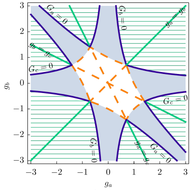
Figure 1: Diagram of solutions for the nodal lines of $E_{g0}$ and $E_{g1}$ near the Dirac point, with $E_{g0},E_{g_{1}}$ taken from Eq. (15) and Eq. (16), respectively. In the solid (blue) regions, there are nodal lines near the Dirac point. The dark solid (blue) borders indicate that there are nodal lines through the Dirac point. When two eigenvalues of $g_{0}$ and $g_{1}$ are equal along the light solid (green) lines, there are nodal rings in $E_{g1}$. The hatched (green) regions are where nodal rings also form when the eigenvalues are not strictly equal. Analytical forms of the solutions are obtained perturbatively near light solid (green) lines as in Eq. (22a). There are no nodal lines along the dashed curves and lines. The directions $g_{a}=0$, $g_{b}=-g_{a}$, and $g_{b}=0$ bisecting the dark (blue) regions correspond to the cases in Table 1.

Clearly, the nodal rings do not appear or disappear discontinuously as we vary the eigenvalues. Instead, we expect that there be a region around the lines of equal eigenvalues in Fig. 1 for which nodal rings exists in the spectrum of $E_{g1}$. We can see this for $g_{b}\gtrsim 1/\sqrt{2}$, where we expect the rings to be close to the Dirac points. For $g_{b}\approx g_{c}$, we can use $\mathbf{v}\approx v\mathbf{k}$ and $\mu\approx B\mathbf{k}^{2}/2$ to find to the lowest-order in $\epsilon:=(g_{c}-g_{b})/g_{b}$ that, when projected to the $b$-$c$ plane, the nodal rings form an ellipse

$$\zeta_{b}k_{b}^{2}+\zeta_{c}k_{c}^{2}=\zeta_{a}k_{a0}^{2}\,,$$ (21a)

where

$$k_{a0}^{2} =(2g_{b}^{2}-1)\frac{4v^{2}}{3B^{2}}\,,$$ (21b)

$$\zeta_{a} =2+\epsilon\,,~{}\zeta_{b}=1+\frac{4}{3}\epsilon\,,~{}\zeta_{c}=1+\frac{4g_{b}^{2}-5}{3(2g_{b}^{2}-1)}\epsilon\,.$$ (21c)

In the full $\mathbf{k}$ space, the nodes are found on the surface

$$k_{a}^{2}=k_{a0}^{2}+A(k_{c})\epsilon\,,$$ (22a)

where

$$A(k_{c})=\frac{5g_{b}^{2}-1}{3(2g_{b}^{2}-1)}k_{c}^{2}-\frac{4}{3}k_{a0}^{2}\,.$$ (22b)

When $g_{b}=g_{c}>1/\sqrt{2}$, $\epsilon=0$ exactly and we find a circular nodal ring with radius $\sqrt{2}|k_{a0}|$ in the $b$-$c$ planes at $k_{a}=\pm k_{a0}$. We have checked numerically that nodal rings exist for the hatched (green) regions in Fig. 1.

On the lattice, the growing effect of $\mu(\mathbf{k})$ away from the Dirac point can cause the nodal lines of $E_{g1}$ to close into an $\infty$ shape. The nodal lines of $E_{g0}=\pm|\mu|$, on the other hand, continue away from the Dirac point to the Brillouin zone edge. In Figs. 2 and 3, we plot typical dispersions exemplifying the topology of nodal lines.

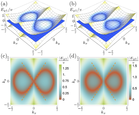
Figure 2: The energy bands for $g_{1}=\text{diag}(g_{a},0,-g_{a})$ with $g_{a}=1.5$ (in the dark blue region with $g_{b}=0$ in Fig. 1 and second row of Table 1) with the principal axes $(a,b,c)=(x,y,z)$. The energy of the two central bands are shown in (a,b) in units of $v$, and the planes show the surface of zero energy. In (a,c), $m=0$ and the $\infty$-shaped nodal lines go through the Dirac point of $E_{g1}(k_{x},k_{y},\pm k_{x})$. In (b,d), $m=0.2v$ and the nodal lines are gapped out at the Dirac point and turn into rings. The dashed lines in density plots (c,d) show the nodal directions $k_{y}=\pm\sqrt{2g_{a}^{2}-1}k_{x}$ through the Dirac point. We have assumed $B=v$ everywhere.

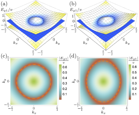
Figure 3: The energy bands for $g_{1}=g_{b}\,\text{diag}(-2-\epsilon,1,1+\epsilon)$ with $g_{b}=0.75$ and (a,c) $\epsilon=0$, (b,d) $\epsilon=0.04$, respectively, on and near the line $g_{b}=g_{c}$ in Fig. 1 with the principal axes $(a,b,c)=(x,y,z)$. The energy of the two central bands in (a,b) are in units of $v$ and show nodal rings of $E_{g1}(k_{x},k_{y},k_{z})$ (a) on the planes $k_{x}=\pm k_{x0}=\pm(2v/B)\sqrt{(2g_{b}^{2}-1)/3}=0.41$ and (b) $k_{x}=\pm\sqrt{k_{x0}^{2}+A(k_{z})\epsilon}$, see Eqs. (22a-22b). The nodal rings shown on the density plots match well with the dashed (c) circle of radius $\sqrt{2}|k_{x0}|=0.58$ and (d) ellipse defined in Eq. (21a). We have assumed $m=0$ and $B=v$ for the lattice parameters.

IV Topology of the band structure

IV.1 Topological invariants

The topologically nontrivial nodal structure of the dispersion for a system with periodic boundary conditions can be characterized by bulk topological invariants. For example, for the $b$ term, the Chern number of the Hamiltonian (8) with respect to the momenta perpendicular to $\mathbf{b}$ and as a function of the momentum component $q$ parallel to $\mathbf{b}$ is $C_{b}(q)=\pm\Theta(|q|<|\mathbf{b}|)$, where the step function $\Theta(s)$ is $1$ if $s$ is true and $0$ otherwise. The nonzero values of $C_{b}$ signify the topological nature of the Weyl semimetal.

For the $g$ term, we utilize the chiral symmetry of the Hamiltonian (14) when $g_{0}=0$ under the chiral operator $C=\mathrm{i}\gamma^{0}\gamma^{5}$,

$$\{H_{g_{1}},C\}=0\,,$$ (23)

to define an integer-valued winding number as a topological invariant. In the chiral eigenbasis, where we have $C=\sigma_{z}\otimes\openone_{2}$ and $H_{g}=\sigma_{x}\otimes h_{x}+\sigma_{y}\otimes h_{y}$, the winding number is defined as

$$W_{C}[H_{g_{1}}]:=\frac{1}{2\pi\mathrm{i}}\oint\frac{\partial\ln\det h(q)}{\partial q}\mathrm{d}q\in\mathbb{Z}\,,$$ (24)

where $h=h_{x}-\mathrm{i}h_{y}$ and $q$ is a cyclic lattice momentum variable. The winding number is a function of $\mathbf{p}$, the momentum perpendicular to the cyclic momentum direction parametrized by $q$. For example, consider a two-dimensional system with momenta $(\mathbf{p},q)$, where $\mathbf{p}$ is normal to $q$. If the system contains a pair of Dirac points with opposite chiralities at $(\pm\mathbf{p}_{0},0)$, the winding number reads $W_{C}(\mathbf{p})=\pm\Theta(|\mathbf{p}|<|\mathbf{p}_{0}|)$. The sign here is determined by the orientation of the Dirac points with respect to the direction of integration over $q$.

We shall now demonstrate the topological characterization of the nodal lines and rings using this winding number under chiral symmetry. In Figs. 4(a) and (b), we sketch the two cases corresponding to Figs. 2(a) and 3(a). Taking $\mathbf{p}$ to be the lattice momentum parallel to the green-shaded plane and the cyclic direction $q$ normal to it, we can see that as the (orange) plane containing $q$ and $\mathbf{p}$ scans the green plane (sampling different $\mathbf{p}$), two Dirac points emerge at the intersection with the nodal lines and move within the plane. Therefore, we expect the winding number $W_{C}(\mathbf{p})=\pm 1$ when $\mathbf{p}$ is sampling the area enclosed by the nodal lines, as sketched by the black and white shaded areas on the green plane. As the planes are rotated, the existence of other nodal lines and rings can lead to a partial cancellation of the winding number, since they contribute opposite signs to overlapping areas of $\mathbf{p}$.

We show the results of a numerical calculation of the winding numbers in Figs. 4(c) and 4(d) corresponding to the cases shown in panels (a) and (b), respectively, of the same figure. The parametrization of the plane of $\mathbf{p}$ in Fig. 4(c) is the same as that used in Fig. 2(a). In Fig. 4(d), the plane of $\mathbf{p}$ is tilted by 45^∘ in the $k_{x}$-$k_{y}$ plane compared to Fig. 4(a) so as to resolve the two nodal rings in the spectrum. As expected, the partial overlap of the two rings at this angle leads to an area with winding number $+1-1=0$.

IV.2 Surface states

For a topological system with open boundaries, surface bound states may arise depending on the surface orientation and the nature of the bulk topology. For example, for the Weyl semimetal with $\mathbf{b}\neq 0$ (see Sec. III.1), the generic dispersion for a boundary that is not orthogonal to $\mathbf{b}$ is an energy surface terminating at a contour that contains the projections of Weyl nodes on the boundary and whose curvature depends on the direction of the boundary. Thus, as is well-known, generic constant-energy contours for bound states on such open boundaries are open “Fermi arcs” [8] terminating on the contour containing the Weyl-node projections.

The topological winding number $W_{C}$ calculated in the previous section corresponds to zero-energy bound states on surfaces terminating the bulk normal to the direction of the cyclic momentum $q$. These bound states are eigenstates of the chiral operator with an eigenvalue equal to $\mathrm{sgn}(W_{C})$ and, thus, their energy is pinned to zero by the chiral symmetry. Therefore, with open boundary conditions on surface terminations parallel to the green planes in Figs. 4(a) and (b), we expect to obtain zero-energy surface bound states for all momenta $\mathbf{p}$ along the surface for which $W_{C}(\mathbf{p})\neq 0$. Such surface bound states form a flat band over a finite area of $\mathbf{p}$ and, thus, have been called “drumhead” surface states.

The existence and the properties of such surface bound states can be studied in a number of ways that incorporate the physics near the boundary. In the continuum formulation, one needs to impose the boundary conditions judiciously so that the resulting Hamiltonian is self-adjoint [117, 118]. Here, instead, we study surface spectra by terminating the lattice Hamiltonians appropriately to form open boundaries.

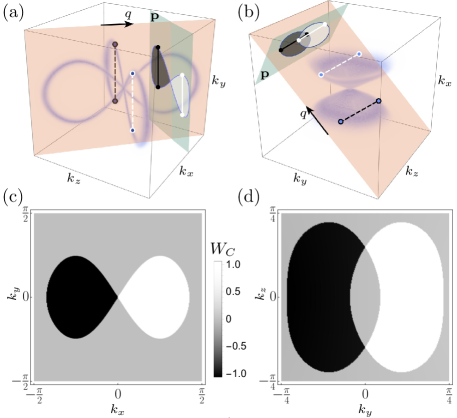
Figure 4: The winding number $W_{C}(\mathbf{p})$ for $g_{1}=\text{diag}(g_{a},0,-g_{a})$ with $g_{a}=1.5$ (a,c) and $g_{1}=g_{b}\,\text{diag}(-2-\epsilon,1,1+\epsilon)$ with $g_{b}=0.75$, $\epsilon=0.04$ (c,d). The plots in (a) and (b) show the calculated nodal lines and rings, respectively, with the cyclic direction $q$ used to define the winding number contained in the (orange) plane normal to the (green) plane of $\mathbf{p}$. As the plane containing $q$ scans values of $\mathbf{p}$, the projection of the nodal lines forms regions with $W_{C}(\mathbf{p})=\pm 1$. In (d), we take $\epsilon=0$. The values of the other parameters are $m=0$ and $B=v$.

To simplify the choice of the boundary along lattice directions and still be able to resolve surface states with opposite chiral eigenvalues, we choose $g_{0}=0$ and

$$g_{1}=g_{a}\begin{pmatrix}1&0&0\\ 0&0&-1\\ 0&-1&-1\end{pmatrix}\,,$$ (25)

where the columns and rows are along the lattice directions $j$. Then, $g_{b}=-\phi g_{a}$, $g_{c}=\phi^{-1}g_{a}$, with the golden ratio $\phi=\frac{\sqrt{5}+1}{2}$, and the eigenvectors of $g_{1}$ are

$$a:\begin{pmatrix}1\\ 0\\ 0\end{pmatrix}\,,\ b:\begin{pmatrix}0\\ \phi^{-1}\\ 1\end{pmatrix}\,,\ c:\begin{pmatrix}0\\ -\phi\\ 1\end{pmatrix}\,.\$$ (26)

Thus, implementing the conditions in Fig. 1, an $\infty$-shaped nodal line is expected for $\sqrt{\phi^{-1}}\approx 0.786<|g_{a}|<1$. For $|g_{a}|=1$, the two $\infty$-shaped nodal lines become tangent and for $|g_{a}|>1$ open into nodal rings. The directions of nodal lines passing through the Dirac point (for $m=0$) and the orientation of the nodal rings are now tilted relative to the lattice directions.

In Figs. 5 and 6, we present numerical results for $g_{a}=0.9$ and $g_{a}=1.3$, respectively, corresponding to the cases with $\infty$-shaped nodal lines and rings. In panel (a) of each figure, the contour of near-zero energy states in the bulk Brillouin zone $(k_{x},k_{y},k_{z})$ are shown as a density plot of $|E_{g_{1}}|$ with $E_{g_{1}}$ of Eq. (16). In panel (b) of each figure, a two-dimensional projection of the minimum energy on the $k_{x}$-$k_{z}$ plane, $E^{\text{min}}_{g_{1}}\equiv\min_{k_{y}}E_{g_{1}}(k_{x},k_{y},k_{z})$, is presented. This illustrates the expected path that pairs of Dirac points traverse as the plane containing the cyclic momentum $q\equiv k_{y}$ used for calculating the winding number scans values of $\mathbf{p}\equiv(k_{x},k_{z})$. This winding number is plotted in panel (c) of each figure.

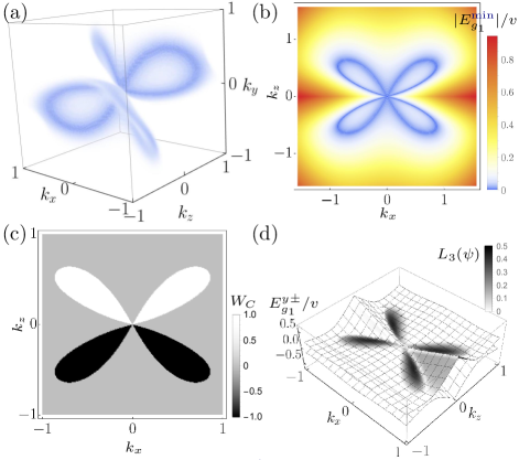
Figure 5: Bulk-boundary correspondence for $H_{g_{1}}$ with $g_{1}$ given by Eq. (25) and $g_{a}=0.9$: (a) The contour of nodal lines; (b) The projection of nodal lines on the $k_{x}$-$k_{z}$ plane showing $E^{\text{min}}_{g_{1}}(k_{x},k_{z})\equiv\min_{k_{y}}E_{g_{1}}(k_{x},k_{y},k_{z})$; (c) the winding number $W_{C}(k_{x},k_{z})$ with cyclic integration along $k_{y}$; (d) the two lowest (closest to zero) energy bands $E_{g_{1}}^{y\pm}$ in an open geometry along the $y$ direction with a lattice size $N_{y}=150$ and color showing the relative wavefunction weight $L_{\delta}(\psi)$ for $\delta=3$ sites near the boundary, see Eq. (27).

Finally, in panel (d) of each figure we plot the lowest two energies (i.e., those closest to zero) in a geometry with open boundaries along the $y$ direction, forming bands $E_{g_{1}}^{y\pm}(k_{x},k_{z})$ as a function of momenta along the periodic directions. These bands contain both bulk and surface bound states. At momenta $\mathbf{p}=(k_{x},k_{z})$ for which there are states in the bulk gap, we would expect the lowest energies to be surface bound states. Such $\mathbf{p}$ should also correspond to nonzero values of $W_{C}(\mathbf{p})$. In order to distinguish bulk and surface bound states, we calculate a measure of edge localization of a wavefunction $\psi$,

$$L_{\delta}(\psi)=\sum_{0\leq|y-y_{b}|\leq\delta}|\psi(y)|^{2}/\left\|\psi\right\|^{2}\,,$$ (27)

where $y_{b}$ are the positions of the boundaries along the $y$ direction, and $\delta$ is the number of sites in the vicinity of the boundary. For a normalized state, $\left\|\psi\right\|^{2}=1$.

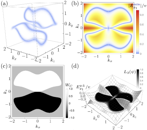
Figure 6: Bulk-boundary correspondence for $H_{g_{1}}$ with $g_{1}$ given by Eq. (25) and $g_{a}=1.3$. Panels show the same data as in Fig. 5.

The results presented in Figs. 5 and 6 clearly show the expected bulk-boundary correspondence between the bulk topological invariant $W_{C}$ and the existence of surface bound states. For $g=0.9$ (Fig. 5), the states in the bulk gap are found close to the surface with half of their weight within a layer of thickness that is $2\%$ of the length of the system in the open direction. For $g=1.3$ (Fig. 6), the bound states have nearly all their weight in the same layer.

V Transport

Topological semimetals are known to exhibit novel transport phenomena. In particular, it has been shown that the Hall conductivity in Weyl semimetals, induced by an applied electromagnetic field, can be derived from the chiral anomaly related to the action in Eq. (1) with nonzero $b$ coefficients [14, 15, 16, 20]. In this view, one may rotate away the $b$ term from the action at tree-level by an appropriate chiral rotation of the Dirac fields. As the partition function is not invariant under the same rotation, quantum corrections induce a nonconservation of chiral charge in the system. These observations provide a strong link between the microscopic theory of Weyl semimetals and the continuum effective action. In this section, we generalize the effective-action approach to transport phenomena and exhaust all possible induced fermion currents generated by quantum corrections at leading order in the coefficients in Eq. (1). In this section, we follow the conventions outlined in Refs. [119, 97], i.e., natural units $\hbar=c=\varepsilon_{0}=1$ are used.

V.1 Fermion current

From the perspective of the continuum action, a systematic way to approach the calculation of induced currents starts with the effective action in $3+1$ Minkowski spacetime

$$Z(A)=\int\mathcal{D}\bar{\psi}\mathcal{D}\psi\,\mathrm{e}^{\mathrm{i}S}\,,$$ (28)

where $S$ is the action of the SME fermion sector stated in Eq. (1), which is minimally coupled to an electromagnetic field. Furthermore, $\mathcal{D}$ indicates a path integral over appropriate Dirac spinor field configurations. The latter $Z(A)$ encodes the response of the system to an electromagnetic background field described by the four-potential $A_{\mu}$. By definition, the induced fermion current is then given by

$$\mathinner{\langle{j^{\mu}}\rangle} =\frac{\int\mathcal{D}\bar{\psi}\mathcal{D}\psi\left[\bar{\psi}\Gamma^{\mu}\psi\right]\mathrm{e}^{\mathrm{i}S}}{\int\mathcal{D}\bar{\psi}\mathcal{D}\psi\,\mathrm{e}^{\mathrm{i}S}}$$

$$=\frac{1}{Z(A)}\left(-\mathrm{i}\frac{\delta}{\delta A_{\mu}(x)}\right)Z(A)\,.$$ (29)

In the latter formula, $\Gamma^{\mu}$ is defined as in Eq. (1), $\frac{\delta}{\delta A_{\mu}}$ denotes the functional derivative for $A_{\mu}$, and we have set the charge $q=1$. The low-energy fluctuations around the vacuum are therefore obtained by integrating out the fermion fields:

$$Z(A) =\int\mathcal{D}\bar{\psi}\mathcal{D}\psi\,\exp\left(\mathrm{i}\int\mathrm{d}^{4}x\,\bar{\psi}\Delta_{A}\psi\right)$$

$$=\det(\Delta_{A})\,,$$ (30)

with the modified Dirac operator $\Delta_{A}$ based on Eq. (1) and minimally coupled to $A_{\mu}$. In the limit of a weak electromagnetic coupling, this form of the effective action can be expanded as a series in powers of $A_{\mu}$ or, equivalently, in powers of the electromagnetic coupling:

$$Z(A)=\det(\Delta)e^{\mathcal{S}(A)}\,,$$ (31a)

where $$\Delta=\mathrm{i}\not{\partial}-m$$ is the standard Dirac operator and

$$\mathcal{S}(A)=-\sum_{n=1}^{\infty}\frac{(-\mathrm{i})^{n}}{n}\int\mathrm{d}x_{1}\cdots\mathrm{d}x_{n}\,f(x_{1},x_{2}\dots x_{n})\,,$$ (31b)

with

$$f(x_{1},x_{2}\dots x_{n}) =\mathrm{tr}[\not{A}(x_{1})G_{F}(x_{2}-x_{1})\cdots$$

$$\phantom{{}={}}\quad\times\not{A}(x_{n})G_{F}(x_{1}-x_{n})]\,.$$ (31c)

Here, $\not{A}:=\gamma^{\mu}A_{\mu}$ and $G_{F}$ is the fermion propagator formally containing corrections from coefficients for Lorentz violation at all orders. The trace is computed with respect to the matrix structure in spinor space. Using this form of the effective action, the leading and sub-leading terms in the electric charge contributing to the induced current are given by

$$\mathinner{\langle{j^{\mu}}\rangle}=\Pi^{\mu\nu}A_{\nu}+\mathrm{V}^{\mu\lambda\kappa}A_{\lambda}A_{\kappa}\,,$$ (32)

where $\mathrm{i}\Pi^{\mu\nu}$ is the vacuum polarization at order $q^{2}$ and $\mathrm{i}\mathrm{V}^{\mu\lambda\kappa}$ is the three-photon vertex correction defined as the sum of all one-particle-irreducible diagrams contributing to the two- and three-point correlation functions in the effective theory, respectively. Note that we have ignored the first-order term in $Z(A)$, which is linear in $A_{\mu}$. In QED, this term vanishes due to Furry’s theorem. In general, it does not vanish for each of the controlling coefficients in Eq. (1). However, at leading order it does so for all coefficients that can give a nonzero contribution to the induced current. For further details regarding the calculation of induced currents, see also Refs. [120, 121].

Thus, the linear and quadratic response for any given coefficient in Eq. (1) can be evaluated simply by computing the modified vacuum polarization or vertex function either by perturbative calculation or otherwise. In this work, we will focus only on the linear response and truncate at leading order in both the electromagnetic coupling and coefficients for Lorentz violation. In the perturbative approach, the response is given by the one-loop vacuum polarization with first-order corrections from coefficients for Lorentz violation. Incorporating the C, P, and T properties of each coefficient in Eq. (1), the generalization of Furry’s theorem reveals that the only coefficients which give a nonzero contribution to the induced linear response at this order are the $b$, $g$, and $c$ terms [97]. We note that by the same logic only the $d$ and $H$ terms are potentially relevant for nonlinear response. However, it was previously found by explicit calculation that these contributions to the modified vertex function vanish [98]. Since all other coefficients in Eq. (1) may be neglected in Lorentz-violating QED due to field redefinitions, our results presented in this section encompass all possible effects in the low-energy response of the system at leading order in Lorentz violation. While the result for the $b$ term has already been widely explored in the context of Weyl semimetals, we establish the method of the effective action outlined here by reproducing known results which have been calculated by independent methods.

Figure 7: Diagrams contributing to the one-loop modified vacuum polarization at leading order in $g$. Effective vertices are indicated by ‘$\bullet$’ and denote a Lorentz-violating vertex insertion. See Ref. [97] for details.

V.2 Chiral anomaly of the $\boldsymbol{b}$ term

Recall from the previous section that the linear induced current is related to the vacuum polarization of the underlying theory. In the case of $b^{\mu}\neq 0$, the vacuum polarization has been previously calculated [48]. The Hall conductivity for spacelike $b^{\mu}$ with $\mathbf{b}^{2}<m^{2}$ is known to vanish [16]. Thus, we consider the regime $\mathbf{b}^{2}>m^{2}$ characterized by the following nonzero contribution:

$$\mathrm{i}\Pi^{\mu\nu}_{b}=\frac{1}{2\pi^{2}}\epsilon^{\mu\nu\alpha\beta}b_{\beta}p_{\alpha}\sqrt{1-\frac{m^{2}}{|b^{2}|}}\,.$$ (33)

It is worth commenting that this result is ambiguous with respect to the chosen regularization scheme and could be shifted by an undetermined constant [3, 46, 47, 49, 48, 50]. However, the additional microscopic details in the condensed-matter setting, in particular the requirement that the Hall current vanish for spacelike $b_{\mu}$, enforce this constant to be zero. For an extensive discussion, see Ref. [12].

Equation (33) immediately gives the induced current

$$\mathinner{\langle{j^{\mu}}\rangle} =\Pi_{b}^{\mu\nu}A_{\nu}(p)$$

$$=\frac{1}{2\pi^{2}}\sqrt{1-\frac{m^{2}}{|b^{2}|}}\epsilon^{\mu\nu\alpha\beta}b_{\beta}(-\mathrm{i}p_{\alpha})A_{\nu}(p)$$

$$=\frac{1}{4\pi^{2}}\sqrt{1-\frac{m^{2}}{|b^{2}|}}\epsilon^{\mu\nu\alpha\beta}b_{\beta}F_{\alpha\nu}\,,$$ (34)

where $F_{\mu\nu}=\partial_{\mu}A_{\nu}-\partial_{\nu}A_{\mu}$ is the electromagnetic field strength tensor in configuration space. For $m^{2}=0$, this agrees with the result obtained via calculation of the chiral anomaly using the Fujikawa method [15] where the latter is given in position space. From Eq. (34), we can easily identify the conductivity of the medium generated by $b^{\mu}$ from the spatial components of the current via $\mathinner{\langle{j^{i}}\rangle}=\sigma^{ij}E_{j}$. Using $\mathbf{E}=-\nabla\phi-\frac{\partial\mathbf{A}}{\partial t}$ and taking the $x$ component of the current, we obtain the well-known Hall conductivity

$$\sigma^{xy}=\frac{1}{2\pi^{2}}{\sqrt{|b^{2}|-m^{2}}}\epsilon^{xyl}\hat{b}_{l}\,,$$ (35)

where $\hat{b}_{l}$ is the $l$-th component of the unit vector $\hat{\mathbf{b}}\equiv\mathbf{b}/|\mathbf{b}|$ pointing along the spatial part $\mathbf{b}$.

V.3 Novel effects of the $\boldsymbol{g}$ term

We proceed now to the calculation of the induced fermion current associated with the $g$ term. Before presenting the main results, it is worth pointing out a few subtleties. Recall from Eq. (5) in Sec. II that the $g$ term can be decomposed into three irreducible representations of the Lorentz group, with the fully antisymmetric part $g^{(A)}_{\mu}$, the trace piece $g_{\mu}^{(T)}$, and the mixed-symmetry part $g^{(M)}_{\kappa\lambda\mu}$. The induced current generated by $g^{(A)}_{\mu}$ is redundant with that of the $b$ term. This can be understood from the fact that $mg^{(A)}_{\mu}$ can be rotated to a $b$-like contribution due to the field redefinitions mentioned in Sec. II. As was also described, the trace component $g^{(T)}_{\mu}$ is unphysical and can also be removed from Eq. (1) without loss of generality. Thus, any new and physically relevant result must come from $g^{(M)}_{\kappa\lambda\mu}$, which was our initial motivation for setting $g^{(A)}_{\mu}=g^{(T)}_{\mu}=0$ starting from Eq. (13).

The one-loop vacuum polarization is straightforward to compute in the perturbative regime via Feynman diagrams. In Fig. 7, we show the diagrams needed for the modified vacuum polarization where vertices corresponding to an insertion of $g^{(M)}_{\kappa\lambda\mu}$ are denoted by the symbol ‘$\bullet$’. Note that while the first class of diagrams, $(1)$ and $(2)$, involve modified QED vertices, diagrams $(3)$ and $(4)$ involve a chirality flip on the internal fermion line. Thus, it is expected that the induced current be proportional to $m$ in contrast to the corresponding results generated by $b$. For a complete list of the associated Feynman rules, see Ref. [97].

Proceeding with standard techniques to calculate the loop, we find

$$\mathinner{\langle{j_{\mu}}\rangle}=\Pi_{\mu\nu}A^{\nu}=-\frac{\mathrm{i}m}{2\pi^{2}}\mathcal{F}(p^{2},m^{2})\left[g^{(M)}_{\mu\nu\alpha}p^{2}+p^{\lambda}\left(p_{\nu}g^{(M)}_{\lambda\mu\alpha}-p_{\mu}g^{(M)}_{\lambda\nu\alpha}\right)\right]p^{\alpha}A^{\nu}\,,$$ (36a)

where we introduced a dimensionless parameter $$x:=\sqrt{p^{2}}/2m$$ as well as a dimensionless function

$$p^{2}\mathcal{F}(p^{2},m^{2}):=\hat{\mathcal{F}}(x)\,,$$ (36b)

such that

$$\hat{\mathcal{F}}(x)=1-\frac{\ln\left[1+2x(\sqrt{x^{2}-1}-x)\right]}{2x\sqrt{x^{2}-1}}=\begin{cases}1-\frac{\ln[1+2|x|(|x|+\sqrt{|x^{2}|+1})]}{2|x|\sqrt{|x^{2}|+1}}\,,&x^{2}<0\\ ~{}\\ 1-\frac{\sin^{-1}(x)}{x\sqrt{1-x^{2}}}\,,&0<x^{2}<1\\ ~{}\\ 1-\frac{\mathrm{i}\pi+\ln|1+2x(\sqrt{x^{2}-1}-x)|}{2x\sqrt{x^{2}-1}}\,,&x^{2}>1\,.\end{cases}$$ (36c)

Note that $\hat{\mathcal{F}}(|x|\to 0)=2|x|^{2}/3+\mathcal{O}(|x|^{4})$ and $\hat{\mathcal{F}}(|x|\to\infty)=1+\mathcal{O}[\ln|x|/|x|^{2}]$ for $x^{2}<0$ as well as $\hat{\mathcal{F}}(x\to 0)=-2x^{2}/3+\mathcal{O}(x^{4})$ and $\hat{\mathcal{F}}(x\to\infty)=1+\mathcal{O}[\ln(x)/x^{2}]$ for $x^{2}>0$. It is worthwhile to note that this result is finite and thus there are no ambiguities related to divergences or the regularization scheme. This can be understood from the momentum structure appearing in the vacuum polarization. Note that each factor in Eq. (36a) appears with three factors of momenta. Thus, any divergence related to the vacuum polarization generated would need to be absorbed by a corresponding counterterm proportional to the $g$ term, three factors of $\partial_{\mu}$, and two factors of $A_{\mu}$. However, it is clear that there is no such counterterm that would be gauge-invariant and renormalizable. Thus, in the minimal SME, defined by Eq. (1), which is gauge-invariant and renormalizable by construction, no such divergence can appear. Additionally, it should be understood that this result is valid for any irreducible component of $g_{\mu\nu\alpha}$, and we have simply assumed that $g^{(A)}_{\mu}=g^{(T)}_{\mu}=0$ in the final result so that $g_{\mu\nu\alpha}=g^{(M)}_{\mu\nu\alpha}$.

We note that while $\mathinner{\langle{j^{\mu}}\rangle}$ is a gauge-invariant quantity, the same is not obvious of the right-hand side of Eq. (36a). Using the definition of the electromagnetic field-strength tensor $F^{\mu\nu}$ in momentum space, we can recast Eq. (36a) in a way where gauge invariance is manifest:

$$\mathinner{\langle{j_{\mu}}\rangle}=\frac{m}{2\pi^{2}p^{2}}\hat{\mathcal{F}}(x)\left(g^{(M)}_{\mu\nu\alpha}p_{\lambda}-\frac{1}{2}{g^{(M)}_{\lambda\nu\alpha}}p_{\mu}\right)p^{\alpha}F^{\lambda\nu}\,.$$ (37)

Following the discussion of Sec. III.1, it is of interest to make the connection of this result to the components of $g^{\kappa\lambda\nu}$ which are relevant in the Hamiltonian formulation of the model, i.e., when $g^{(M)}_{\kappa\lambda 0}=0$.

Parametrizing in terms of the matrices $g_{0}$ and $g_{1}$ of Eqs. (13a) and (13b) and denoting the momentum four-vector $p^{\mu}=(\omega,\mathbf{p})$, the charge density $\mathinner{\langle{\rho}\rangle}\equiv\mathinner{\langle{j^{0}}\rangle}$ and the spatial current $\mathinner{\langle{\mathbf{j}}\rangle}$ take the form

$$\mathinner{\langle{\rho(\omega,\mathbf{p})}\rangle} =\frac{m\omega\hat{\mathcal{F}}(x)}{2\pi^{2}p^{2}}\left[(g_{0}\mathbf{p})\cdot\mathbf{E}+(g_{1}\mathbf{p})\cdot\mathbf{B}\right]\,,$$ (38a)

$$\mathinner{\langle{\mathbf{j}(\omega,\mathbf{p})}\rangle} =\frac{m\hat{\mathcal{F}}(x)}{2\pi^{2}p^{2}}\mathbf{p}\left[(g_{0}\mathbf{p})\cdot\mathbf{E}+(g_{1}\mathbf{p})\cdot\mathbf{B}\right]\,.$$ (38b)

Here, we have assumed that the applied electromagnetic background field obeys the source-free Maxwell equations.

Thus, $g_{0}$ and $g_{1}$ characterize, respectively, the electric conductivity tensor and the magnetoelectric response of the system. Remarkably, for $g_{1}\neq 0$ the application of a magnetic field pulse can result in both a charge density and an electric current. For example, for static electromagnetic fields $E(\mathbf{r})$ and $B(\mathbf{r})$, we find $\mathinner{\langle{\rho}\rangle}=0$ and

$$\mathinner{\langle{\mathbf{j}}\rangle}=\frac{m}{2\pi^{2}}\left[\boldsymbol{\nabla}(g_{0}\boldsymbol{\nabla})\cdot{\mathbf{E}}^{\prime}+\boldsymbol{\nabla}(g_{1}\boldsymbol{\nabla})\cdot{\mathbf{B}}^{\prime}\right]\,,$$ (39a)

where the fields are obtained via $${\mathbf{E}}^{\prime}(\mathbf{r})=\int\mathrm{d}^{3}\mathbf{r}^{\prime}\,\tilde{\mathcal{F}}(\mathbf{r}-\mathbf{r}^{\prime})\mathbf{E}(\mathbf{r}^{\prime}) {\mathbf{B}}^{\prime}(\mathbf{r}) x^{2}<0 |x|\to 0 |x|\to\infty$$ and similarly for . The integration kernel follows from a Fourier transform of Eq. (36b). We employ the following asymptotic form of Eq. (36b) that is valid for and has the correct asymptotic behavior for and :

$$\hat{\mathcal{F}}(x)|_{x^{2}<0}\sim\frac{|x|^{2}}{|x|^{2}+3/2}\,.$$ (39b)

Then,

$$\tilde{\mathcal{F}}(\mathbf{r})=\int\frac{\mathrm{d}^{3}\mathbf{p}}{(2\pi)^{3}}\,\mathcal{F}(-|\mathbf{p}|^{2},m^{2})\mathrm{e}^{-\mathrm{i}\mathbf{p}\cdot\mathbf{r}}\approx\frac{\mathrm{e}^{-\sqrt{6}m|\mathbf{r}|}}{4\pi|\mathbf{r}|}\,.$$ (39c)

Thus, the kernel is approximately a screened Coulomb potential.

V.4 The $\boldsymbol{c}$ term

To complete the list of coefficients for Lorentz violation that give a nonzero induced current at leading order in Lorentz violation, we consider the $c$ term. In this case, the antisymmetric and trace components of $c$ can be removed via appropriate field redefinitions following a similar reasoning as that for the $g$ term. Thus, in our derivation we retain only the symmetric, traceless components of $c^{\mu\nu}$. The one-loop vacuum polarization at leading order in Lorentz violation is then given by

$$\mathinner{\langle{j^{\mu}}\rangle}=-\frac{1}{6\pi^{2}}\left\{\hat{\mathcal{K}}_{1}(x)\left[c^{\mu\nu}p^{2}-p^{\mu}(p\cdot c)^{\nu}-p^{\nu}(p\cdot c)^{\mu}\right]+{p\cdot c\cdot p}\left(\hat{\mathcal{K}}_{2}(x)\eta^{\mu\nu}+\hat{\mathcal{K}}_{3}(x)\frac{p^{\mu}p^{\nu}}{p^{2}}\right)\right\}A_{\nu}\,,$$ (40a)

with the dimensionless functions

$$\hat{\mathcal{K}}_{1}(x) =\left[\frac{5}{3}+\frac{1}{\epsilon}+\ln\left(\frac{\bar{\mu}^{2}}{m^{2}}\right)\right]+\left(1+\frac{1}{2x^{2}}\right)\hat{\mathcal{C}}(x)+\frac{1}{x^{2}}\,,$$ (40b)

$$\hat{\mathcal{K}}_{2}(x) =\left[\frac{2}{3}+\frac{1}{\epsilon}+\ln\left(\frac{\bar{\mu}^{2}}{m^{2}}\right)\right]+\frac{4x^{4}-2x^{2}+1}{4x^{2}(x^{2}-1)}\hat{\mathcal{C}}(x)-\frac{1}{2x^{2}}\,,$$ (40c)

$$\hat{\mathcal{K}}_{3}(x) =-\frac{3}{4x^{2}(x^{2}-1)}\hat{\mathcal{C}}(x)+1+\frac{3}{2x^{2}}\,,$$ (40d)

where, again, $$x=\sqrt{p^{2}}/2m \bar{\mu}^{2}=\mu^{2}_{r}\mathrm{e}^{\gamma_{E}}/4\pi \gamma_{E} \mu_{r}$$ and we have used dimensional regularization to evaluate the divergent pieces of the diagram, thus introducing the unphysical mass scale , with the Euler-Mascheroni constant. Furthermore, is an arbitrary reference mass scale needed for dimensional consistency. For brevity, we have also introduced the dimensionless function

$$\hat{\mathcal{C}}(x)=\frac{\sqrt{x^{2}-1}}{x}\ln\left[1+2x\left(\sqrt{x^{2}-1}-x\right)\right]\,.$$ (40e)

Note that $\hat{\mathcal{C}}(x\to 0)=-2+2x^{2}/3+\mathcal{O}(x^{4})$ and $\hat{\mathcal{C}}(x\to\infty)=\ln[-1/(4x^{2})]+\mathcal{O}(\ln[-1/(4x^{2})]/x^{2})$.

In this case, there are divergent pieces that appear in the loop evaluation. The divergent pieces can be removed by appropriate counterterms in a gauge-invariant, renormalizable way [97]. One possible option would be to utilize the on-shell renormalization scheme, which has the advantages that the fermion mass $m$ appearing in the Lagrangian retains the meaning of the physical mass as opposed to the running mass and effectively removes the unphysical mass scale $\bar{\mu}^{2}$ from the vacuum polarization. In effect, the Lagrangian parameters will evolve with the choice of reference scale [97]. Irrespective of the choice of renormalization scheme the full expression we obtain is in agreement with the general considerations presented in Ref. [3].

Finally, we come to the form of the induced current in which gauge invariance is manifest:

$$\mathinner{\langle{j^{\mu}}\rangle} =-\frac{\mathrm{i}}{8\pi^{2}}\bigg{[}\hat{\mathcal{K}}_{1}(x)c^{\mu\alpha}p^{\nu}F_{\nu\alpha}+\hat{\mathcal{K}}_{2}(x)c^{\alpha\beta}p_{\beta}F^{\mu}_{\phantom{\mu}\alpha}$$

$$\phantom{{}={}}\hskip 31.2982pt+\hat{\mathcal{K}}_{3}(x)c^{\alpha\beta}p_{\beta}p^{\mu}p^{\nu}F_{\alpha\nu}\bigg{]}\,.$$ (41)

Taking into account the components relevant to the Hamiltonian formulation, where $c^{\mu 0}=0$, we find that the charge and current densities can be written as

$$\mathinner{\langle{\rho}\rangle} =-\mathrm{i}\frac{\hat{\mathcal{K}}_{2}(x)}{8\pi^{2}}c_{ij}p_{j}E_{j}\,,$$ (42a)

$$\mathinner{\langle{j^{k}}\rangle} =-\mathrm{i}\frac{\hat{\mathcal{K}}_{2}(x)}{8\pi^{2}}\epsilon^{kil}c_{ij}p_{j}B_{l}\,,$$ (42b)

respectively.

VI Summary and outlook

This paper proposes a correspondence between the field-theoretic description of emergent Lorentz symmetry in condensed-matter systems and the SME framework, which is the comprehensive effective field theory for Lorentz violation appropriate for studies of fundamental theories of spacetime and matter. The correspondence provides a foundation for classifying and characterizing general quasiparticle excitations using the SME, and conversely it implies that features of emergent Lorentz symmetry in certain materials can yield insights into Lorentz-violating properties of spacetime and matter.

The body of this work focuses on emergent Lorentz invariance in three-dimensional Dirac materials as viewed from the general perspective offered by the SME. The correspondence with the SME enables the classification of field-theoretic terms in the action governing departures from emergent Lorentz symmetry, according to the mass dimension and spinor structure of the operator. This permits the construction of lattice Hamiltonians that incorporate all types of Lorentz violations around the original Lorentz-symmetric Dirac nodes of the material.

Part of our investigations involve the study of changes to the Dirac nodal structure arising from the presence of specific types of SME coefficients for Lorentz violation. We discuss a modification of the Dirac operator, known as the $b$ term and previously examined in the literature, which leads to a Weyl semimetal with two nodes of opposite chirality separated in momentum and/or energy. We also consider another modification of the Dirac operator called the $g$ term, previously unexplored in the condensed-matter context, that describes Dirac nodal semimetals with intersecting Dirac lines and/or Dirac nodal rings. The bulk topological invariants and the existence and properties of surface bound states are explored. The band structures associated with the $b$ and $g$ terms are strikingly different, a noteworthy feature given that the C-, P-, and T-symmetry properties of the Hamiltonian components involving $(g_{0})_{ij}$ and $(g_{1})_{ij}$ of Eq. (13) are identical to those involving $b_{j}$ and $b_{0}$, respectively, as can be verified from Table 1 of Ref. [97]. The general effective action describing P- or T-symmetry violation in semimetals must therefore incorporate both terms, which generate distinct band structures.

Another part of our investigation concerns the transport coefficients for various types of semimetals. At leading order in perturbation theory, we calculate the transport coefficients for the $b$ and $g$ terms and for another modification of the Dirac operator called the $c$ term. Interestingly, even at perturbatively small values, the $g$ term modifies the Maxwell equations in the material in unconventional ways. In particular, the current- and charge-density response of the material is determined by the second derivatives of nonlocal screened electromagnetic fields, as given in Eqs. (38) and (39).

The correspondence proposed here between deviations from emergent Lorentz symmetry in materials and the SME framework suggests various future research topics spanning condensed-matter and high-energy physics. Several of these arise directly from the approach and results obtained in the present work. For example, the lattice models for a few types of minimal SME coefficients remain to be investigated in detail, including ones such as $c_{\lambda 0}$ and $g_{\kappa\lambda 0}$ that are disregarded here to minimize complications in the Hamiltonian description. The associated band structures, topological invariants, and bound surface states would be interesting to establish. An intriguing open issue in the general case is the identification of appropriate boundary conditions and the resulting surface states in the presence of Lorentz-violating terms. For the $b$ term associated with Weyl semimetals, the most general boundary conditions can be found through self-adjoint extensions of the Hamiltonian [118], and it would be valuable to generalize this method to other SME coefficients.

Our study of transport coefficients could also be broadened. While we have exhausted the list of minimal coefficients for Lorentz violation that lead to a nonvanishing induced current at leading order, certain SME coefficients in the action (1) may generate a nonvanishing fermion current from the vacuum polarization when evaluated at second and higher orders in Lorentz violation. Arguments analogous to Furry’s theorem suggest that a nonzero current is to be expected from contributions such as the $d$ and $H$ terms in Eq. (1). Second-order effects from the $b$, $c$, and $g$ terms may also induce a nonlinear fermion current through the modified vertex function. It would be of interest to investigate the transport coefficients nonperturbatively, by including the full dispersion for large SME coefficients.

Intriguing open issues in the broader context are also suggested by the correspondence between the SME and condensed-matter systems. The full SME incorporates additional terms with field operators of mass dimensions $d>4$, along with couplings to all known gauge fields and gravity [62, 63, 64, 65, 4, 66, 67, 68]. These terms represent a large set of modifications to the Dirac operator that as yet remain unexplored in the condensed-matter context, so there is considerable potential for the discovery and possibly even the design of interesting and novel materials emergent Lorentz symmetry. In the other direction, condensed-matter systems offer prospects for informing SME physics. Issues in the SME such as the conditions for quantum stability, the interpretation of scenarios with large coefficients for Lorentz violation, and the understanding of ambiguities in radiative corrections could be addressed in the context of materials with departures from emergent Lorentz symmetry, both via methods from condensed-matter theory and through material realizations of SME systems in the laboratory.

Another interesting angle to pursue is the connection to Finsler geometry. In the SME, the trajectory of the centroid of a fermion or scalar wavepacket in the presence of Lorentz violation is known to correspond to a geodesic in a Riemann-Finsler spacetime [53, 122, 123, 124, 125, 126, 127, 128, 129]. We therefore anticipate that Finsler geometry underlies the motion of quasiparticles in Dirac and Weyl semimetals and other materials exhibiting departures from emergent Lorentz symmetry. This situation offers the potential for interdisciplinary advances in several directions. For example, results in Finsler geometry can be expected to provide insights into the physics of various materials with emergent Lorentz symmetry, while these systems in turn provide analogue models and laboratory realizations for challenging mathematical issues. Overall, the numerous topics open for investigation across these seemingly disparate subjects offer rich prospects for future advances.