Chen, Fampa and Lee

Computing with convex relaxations for MESP

On computing with some convex relaxations
for the maximum-entropy sampling problem

Zhongzhu Chen University of Michigan, zhongzhc@umich.edu Marcia Fampa Universidade Federal do Rio de Janeiro, fampa@cos.ufrj.br Jon Lee University of Michigan, jonxlee@umich.edu

Based on a factorization of an input covariance matrix, we define a mild generalization of an upper bound of Nikolov (2015) and Li and Xie (2020) for the NP-Hard constrained maximum-entropy sampling problem (CMESP). We demonstrate that this factorization bound is invariant under scaling and also independent of the particular factorization chosen. We give a variable-fixing methodology that could be used in a branch-and-bound scheme based on the factorization bound for exact solution of CMESP, and we demonstrate that its ability to fix is independent of the factorization chosen. We report on successful experiments with a commercial nonlinear-programming solver. We further demonstrate that the known “mixing” technique can be successfully used to combine the factorization bound with the factorization bound of the complementary CMESP, and also with the “linx bound” of Anstreicher (2020).

maximum-entropy sampling, convex relaxation, integer nonlinear optimization, mixing bounds

1 Introduction

Let $C$ be a symmetric positive semidefinite matrix with rows/columns indexed from $N:=\{1,2,\ldots,n\}$, with $n>1$. For $0<s<n$, we define the maximum-entropy sampling problem

(MESP) $$\begin{array}[]{ll}z(C,s):=&\max\left\{\operatorname{ldet}C[S(x),S(x)]~{}:~{}\mathbf{e}^{\top}x=s,~{}x\in\{0,1\}^{n}\right\},\end{array}$$

where $S(x)$ denotes the support of $x\in\{0,1\}^{n}$, $C[S,S]$ denotes the principal submatrix indexed by $S$, and $\operatorname{ldet}$ denotes the natural logarithm of the determinant.

This problem, which has application to contracting environmental monitoring networks (see Zidek, Sun, and Le (2000), Caselton and Zidek (1984), Caselton, Kan, and Zidek (1992), Wu and Zidek (1992), Lee (2012), for example), is a mathematical-programming formulation of the NP-Hard problem of finding a subset of $s$ random variables from a Gaussian random $n$-vector having covariance matrix $C$, so as to maximize the “information” (measured by “differential entropy”); see Shewry and Wynn (1987), Ko, Lee, and Queyranne (1995), Sebastiani and Wynn (2000), Lee (2012), Anstreicher (2020), and the many references they contain.

In practical applications, there are often side constraints (e.g., based on budgetary restriction, geographical considerations, etc). In this spirit, for $A\in\mathbb{R}^{m\times n}$ and $b\in\mathbb{R}^{m}$, we further define the constrained maximum-entropy sampling problem

(CMESP) $$\begin{array}[]{ll}z(C,s,A,b):=&\max\left\{\textstyle\vphantom{\sum_{j\in S}}\operatorname{ldet}C[S(x),S(x)]~{}:~{}\mathbf{e}^{\top}x=s,~{}Ax\leq b,~{}x\in\{0,1\}^{n}\right\}.\\ \end{array}$$

The main approach for solving MESP and CMESP to optimality is branch-and-bound. Lower bounds are calculated by local search, rounding, etc. Branching is done by deleting a symmetric row/column pair from $C$ for a “down branch” and calculating a Schur complement for an “up branch”. Upper bounds are calculated in a variety of ways. One class of methods uses spectral information; see Ko, Lee, and Queyranne (1995), Lee (1998), Hoffman, Lee, and Williams (2001), Anstreicher and Lee (2004), Burer and Lee (2007). Another class of methods is based on convex relaxations; see Anstreicher, Fampa, Lee, and Williams (1999), Anstreicher (2018, 2020). Recently, Nikolov (2015) and Li and Xie (2020) developed a convex relaxation based on spectral information.

It is easy to check that

$$z(C,s,A,b)=z(C^{-1},n-s,-A,b-A\mathbf{e})+\operatorname{ldet}C~{}.$$

So we have a notion of a complementary CMESP problem

(CMESP-comp) $$z(C^{-1},n-s,-A,b-A\mathbf{e})=$$

$$\qquad\max\left\{\textstyle\vphantom{\sum_{j\in S}}\operatorname{ldet}C^{-1}[S(x),S(x)]~{}:~{}\mathbf{e}^{\top}x=n-s,~{}A(\mathbf{e}-x)\leq b,~{}x\in\{0,1\}^{n}\right\},$$

and complementary bounds (i.e., bounds for the complementary problem plus $\operatorname{ldet}C$) immediately give us bounds on $z(C,s,A,b)$. Some upper bounds on $z(C,s,A,b)$ also shift by $\operatorname{ldet}C$ under complementing, in which case there is no additional value in computing the complementary bound.

It is also easy to check that

$$z(C,s,A,b)=z(\gamma C,s,A,b)-s\log\gamma,$$

where the scale factor $\gamma>0$. So we have a notion of a scaled CMESP problem defined by the data $\gamma C$, $s$, $A$, $b$, and scaled bounds (i.e., bounds for the scaled problem minus $s\log\gamma$) immediately give us bounds on $z(C,s,A,b)$. Some upper bounds on $z(C,s,A,b)$ also shift by $-s\log\gamma$ under scaling, in which case there is no additional value in computing the scaled bound.

In Section 2, we discuss some upper bounds for CMESP. In particular, we present the “factorization bound” for CMESP, as a convex formulation 2.2 of the Lagrangian dual of a nonconvex formulation 2.1, and some of its important properties from a computational point of view. In particular:

• We demonstrate that the factorization bound changes by the same amount as $z(C,s,A,b)$, when $C$ is scaled by some $\gamma>0$.

• We give a variable fixing methodology based on a feasible solution of 2.2. Variable fixing has also been studied for CMESP in the context of other convex relaxations; see Anstreicher, Fampa, Lee, and Williams (1996, 1999, 2001), Anstreicher (2018, 2020).

• We demonstrate that the factorization bound and its ability to fix variables, based on a matrix factorization $C=FF^{\top}$, is independent of the factorization (and so mathematically, it provides the same bound as that of Nikolov (2015) and Li and Xie (2020)).

• We demonstrate that the factorization bound dominates the well-known “spectral bound”.

• Although it is possible to directly attack 2.2 to calculate the factorization bound, it is much more fruitful to work with 2.3, a convex formulation of the Lagrangian dual of 2.2. In connection with this, we provide a mechanism to get a minimum-gap feasible solution of 2.2, relative to a feasible (and possibly non-optimal) solution of 2.3 (which is useful for getting a true upper bound for CMESP). We also describe how to get the gradient of the objective function of 2.3 (under a technical condition), which is necessary for applying any reasonable technique for efficiently solving 2.3.

• We review the 2.4 bound for CMESP, and we present some of its key properties that are useful for computing.

• We review the “mixing” bound of Chen, Fampa, Lambert, and Lee (2021), and we work out a dual formulation for it, as well as a fixing methodology in an important case that generalizes what we can do for 2.3, complementary 2.3, and 2.4.

In Section 3, we discuss the numerical experiments where, using a commercial nonlinear-programming solver, we calculate upper bounds for benchmark instances of MESP from the literature with the three relaxations presented, namely 2.3, complementary 2.3 and 2.4, and with the “mixing” strategy described in Chen, Fampa, Lambert, and Lee (2021). Generally, we found that a commercial nonlinear-programming solver is quite viable for our relaxations, even for 2.3 which may have nondifferentiabilty. Our main findings:

• We compared integrality gaps given by the difference between the upper bounds computed with the relaxations and the lower bounds computed with a greedy/interchange heuristic or with the optimal value when we could obtain it by branch-and-bound. We found that all the three relaxations, 2.3, complementary 2.3, and 2.4, achieve the best bounds for some of the instances, however 2.3 and 2.4 achieve together most of the best bounds.

• We compared the times to solve the relaxations and analyzed the impact of two factors in the times: the smoothness of the objective functions of the relaxations and the ranks of the covariance matrices. The possibility of 2.3 and complementary 2.3 encountering points at which the objective function is nondifferentiable led us to the application of a BFGS-based algorithm to solve these relaxations, and the smoothness of 2.4 results in the application of a Newton-based algorithm to solve it. We see a better convergence of the Newton-based algorithm, resulting in best times for 2.4 and with less variability among the different values of $s$, except for our largest instance with $n=2000$ and a covariance matrix with rank $r=949$. In this case, 2.4 presents the drawback of dealing with an order-$n$ matrix in its objective function, while 2.3 deals with an order-$r$ matrix.

• We demonstrated how the “mixing” procedure can decrease the bounds obtained with the three relaxations when we mix two relaxations that obtain very similar bounds when applied separately. This is mostly observed when we mix 2.3 and 2.4. For the majority of the instances, 2.3 presents better bounds for values of $s$ up to an intermediate value, and for larger values of $s$, 2.4 presents better bounds. For values of $s$ close to this intermediate value, the mixing strategy effectively decreases the bound obtained by each relaxation.

• We demonstrated how the fixing methodology can fix a significant number of variables, especially when applied iteratively, to our largest instance.

In Section 4, we summarize our results and point to future work.

Notation. We let $\mathbb{S}^{n}_{+}$ (resp., $\mathbb{S}^{n}_{++}$) denote the set of positive semidefinite (resp., definite) symmetric matrices of order $n$. We denote by $\lambda_{\ell}(M)$ the $\ell$-th greatest eigenvalue of a matrix $M\in\mathbb{S}^{n}_{+}$ . We denote an all-ones vector by $\mathbf{e}$ and the $i$-th standard unit vector by $\mathbf{e}_{i}$ . For matrices $A$ and $B$ with the same shape, $A\circ B$ is the Hadamard (i.e., element-wise) product, and $A\bullet B:=\operatorname{tr}(A^{\top}B)$ is the matrix dot-product. For a matrix $A$, we denote row $i$ by $A_{i\cdot}$ and column $j$ by $A_{\cdot j}$ .

2 Upper bounds

There are a wide variety of upper bounding methods for CMESP. The tightest bounds, from a practical computational viewpoint, seem to be Anstreicher’s “linx bound” and the “factorization bound”. In this section, we describe and develop these bounds, with an eye on practical and efficient computation.

2.1 Fact

We begin by introducing a mild generalization of a nonconvex programming bound developed by Nikolov (2015) and Li and Xie (2020). Suppose that the rank of $C$ is $r\geq s$. Then we factorize $C=FF^{\top}$, with $F\in\mathbb{R}^{n\times k}$, for some $k$ satisfying $r\leq k\leq n$. We note that this could be a Cholesky-type factorization (i.e., $k:=r$ and $F$ lower triangular), as in Nikolov (2015) and Li and Xie (2020). But it could alternatively be derived from a spectral decomposition of $C$; that is, $C=\sum_{\ell=1}^{r}\lambda_{\ell}v_{\ell}v_{\ell}^{\top}$, where we put $\sqrt{\lambda_{\ell}}v_{\ell}$ as column $\ell$ of $F$, $\ell=1,\ldots,k:=r$. Another very useful possibility is to let $k:=n$, and choose $F$ to be the matrix square root, $C^{1/2}$, which is always symmetric.

Next, for $x\in[0,1]^{n}$, we define $F(x):=\sum_{j\in N}F_{j\cdot}^{\top}F_{j\cdot}~{}x_{j}~{}=F^{\top}\operatorname{Diag}(x)F$ and

$$\begin{array}[]{ll}z_{{\tiny\mbox{Fact}}}(C,s,A,b;F):=&\max\displaystyle\sum_{\ell=1}^{s}\log\left(\lambda_{\ell}(F(x))\right)\\ &\mbox{subject to:}\\ &\quad\mathbf{e}^{\top}x=s,~{}Ax\leq b,~{}0\leq x\leq\mathbf{e}.\end{array}$$

It is easy to check that $z(C,s,A,b)\leq z_{{\tiny\mbox{Fact}}}(C,s,A,b;F)$, for any factorization of $C$ (c.f. Ko, Lee, and Queyranne (1995)). Unfortunately, 2.1 is not a convex program, so it is not a practical relaxation to work with.

2.2 DFact

We define

$$f(\Theta,\nu,\pi,\tau):=-\sum_{\ell=k-s+1}^{k}\log\left(\lambda_{\ell}\left(\Theta\right)\right)+\nu^{\top}\mathbf{e}+\pi^{\top}b+\tau s-s,$$

and the factorization bound

$$\begin{array}[]{ll}z_{{\tiny\mbox{DFact}}}(C,s,A,b;F):=&\min~{}f(\Theta,\nu,\pi,\tau)\\ &\mbox{subject to:}\\ &\quad\operatorname{diag}(F\Theta F^{\top})+\upsilon-\nu-A^{\top}\pi-\tau\mathbf{e}=0,\\ &\quad\Theta\succ 0,~{}\upsilon\geq 0,~{}\nu\geq 0,~{}\pi\geq 0.\end{array}$$

2.2 is equivalent to the Lagrangian dual of 2.1, and it is a convex program. The objective function of 2.2 is analytic at every point $(\hat{\Theta},\hat{\upsilon},\hat{\nu},\hat{\pi},\hat{\tau})$ for which $\lambda_{k-s}(\hat{\Theta})>\lambda_{k-s+1}(\hat{\Theta})$. In fact, we have seen in our experiments, a good solver can get to an optimum, even when this condition fails.

It turns out that the factorization bound for MESP has a close relationship with the spectral bound of Ko, Lee, and Queyranne (1995): $\sum_{\ell=1}^{s}\log\lambda_{\ell}(C)$. First, we establish that like the spectral bound for MESP, the factorization bound for CMESP is invariant under multiplication of $C$ by a scale factor $\gamma$, up to the additive constant $-s\log\gamma$, a property that is not shared with other convex-optimization bounds.

Theorem 2.1

For all $\gamma>0$ and factorizations $C=FF^{\top}$, we have

$$z_{{\tiny\mbox{DFact}}}(C,s,A,b;F)=z_{{\tiny\mbox{DFact}}}(\gamma C,s,A,b;\sqrt{\gamma}F)-s\log\gamma.$$

Proof.

Proof. We simply observe that for every feasible solution $(\hat{\Theta},\hat{\upsilon},\hat{\nu},\hat{\pi},\hat{\tau})$ of 2.2, we have that $(\frac{1}{\gamma}\hat{\Theta},\hat{\upsilon},\hat{\nu},\hat{\pi},\hat{\tau})$ is a feasible solution of 2.2 with $F$ replaced by $\sqrt{\gamma}F$. Then we observe that $\lambda_{\ell}\left(\frac{1}{\gamma}\hat{\Theta}\right)=\frac{1}{\gamma}\lambda_{\ell}(\hat{\Theta})$, for all $\ell$. This mapping between feasible solutions is a bijection, so the result follows. ∎

Because the factorization bound shifts by the same amount as $z(C,s,A,b)$, under scaling of $C$ by $\gamma$, we cannot improve on the factorization bound by scaling. In contrast, the linx bound is very sensitive to the choice of the scale factor, and while we can compute an optimal scale factor for the linx bound (see Chen, Fampa, Lambert, and Lee (2021)), it is a significant computational burden to do so.

Next, we present another useful result that guides practical usage.

Theorem 2.2

Let $C=F_{j}F_{j}^{\top}$, for $j=1,2$, be two different factorizations of $C$, and let $(\hat{\Theta}_{1},\hat{\upsilon},\hat{\nu},\hat{\pi},\hat{\tau})$ be a feasible solution to 2.2, for $F:=F_{1}$. Then, there is a feasible solution $(\hat{\Theta}_{2},\hat{\upsilon},\hat{\nu},\hat{\pi},\hat{\tau})$ to 2.2, for $F:=F_{2}$, such that $f(\hat{\Theta}_{1},\hat{\nu},\hat{\pi},\hat{\tau})=f(\hat{\Theta}_{2},\hat{\nu},\hat{\pi},\hat{\tau})$.

Proof.

Proof.Let $r$ be the rank of $C$, and let $C=\sum_{\ell=1}^{n}\lambda_{\ell}u_{\ell}u_{\ell}^{\top}$ be a spectral decomposition of $C$. Suppose that $C=FF^{\top}$, with $F\in\mathbb{R}^{n\times k}$, and $r\leq k\leq n$. Our preliminary goal is to build a special singular-value decomposition of $F$.

Let $\sigma_{\ell}:=\sqrt{\lambda_{\ell}}$, for $1\leq\ell\leq k$. Now define $v_{\ell}\in\mathbb{R}^{k}$, for $1\leq\ell\leq r$ by $v_{\ell}:=\frac{1}{\sigma_{\ell}}F^{\top}u_{\ell}$.

We can easily check that for $1\leq i\leq\ell\leq r$, we have

$$v_{i}^{\top}v_{\ell}=\frac{1}{\sigma_{i}\sigma_{\ell}}u_{i}^{\top}FF^{\top}u_{\ell}=\frac{1}{\sigma_{i}\sigma_{\ell}}u_{i}Cu_{\ell}=\frac{\lambda_{\ell}}{\sigma_{i}\sigma_{\ell}}u_{i}^{\top}u_{\ell}=\left\{\begin{array}[]{ll}1,&\hbox{ for $i=\ell$;}\\ 0,&\hbox{ for $i<\ell$.}\end{array}\right.$$

That is, $\{v_{\ell}~{}:~{}1\leq\ell\leq r\}$ is a set of $r$ orthonormal vectors in $\mathbb{R}^{k}$. So, for $r<\ell\leq k$, we can now choose $v_{i}$ so as to complete $\{v_{\ell}~{}:~{}1\leq\ell\leq r\}$ to an orthonormal basis of $\mathbb{R}^{k}$.

Next, we have

$$\sum_{\ell=1}^{k}\sigma_{\ell}u_{\ell}v_{\ell}^{\top}=\sum_{\ell=1}^{r}\sigma_{\ell}u_{\ell}v_{\ell}^{\top}=\sum_{\ell=1}^{r}u_{\ell}u_{\ell}^{\top}F=\sum_{\ell=1}^{n}u_{\ell}u_{\ell}^{\top}F=I_{n}F=F$$

(note that above we have use the fact that $\|u_{\ell}^{\top}F\|^{2}=u_{\ell}^{\top}FF^{\top}u_{\ell}=\lambda_{\ell}=0$ for $r<\ell\leq n$, which implies that $u_{\ell}^{\top}F=0^{\top}_{k}$ for $r<\ell\leq n$), and so we can conclude that $F=\sum_{\ell=1}^{k}\sigma_{\ell}u_{\ell}v_{\ell}^{\top}$ is a singular-value decomposition for $F$.

The important takeaway is that the $u_{\ell}\in\mathbb{R}^{n}$ ($1\leq\ell\leq n$) and the nonzero $\sigma_{\ell}$ ($1\leq\ell\leq r$) in the singular-value decomposition that we constructed for $F$ only depend on $C$, not on the particular factorization $C=FF^{\top}$.

It is convenient now to establish that in a factorization matrix $F$, we can without loss of generality take $k=n$, by appending 0 columns to $F$ if needed, and this will not affect the bound $z_{{\tiny\mbox{DFact}}}(C,s,A,b;F)$. Let $\bar{F}:=[F~{}|~{}0_{n\times(n-k)}]$, and consider

$$\bar{\Theta}=\left(\begin{array}[]{cc}\hat{\Theta}&\times\\ \times&\times\\ \end{array}\right)\in\mathbb{S}^{n}_{+}~{}.$$

It is trivial to check that $\bar{F}\bar{\Theta}\bar{F}^{\top}=F\hat{\Theta}F^{\top}$. And by Cauchy’s eigenvalue interlacing inequalities (see Horn and Johnson (1985), for example), we have $\lambda_{\ell+n-k}(\bar{\Theta})\leq\lambda_{\ell}(\hat{\Theta})$, for $1\leq\ell\leq k$. Therefore, we have $z_{{\tiny\mbox{DFact}}}(C,s,A,b;\bar{F})\geq z_{{\tiny\mbox{DFact}}}(C,s,A,b;F)$. In the other direction, suppose that $\hat{\Theta}\in\mathbb{S}^{k}_{+}$ . Now define

$$\bar{\Theta}:=\left(\begin{array}[]{cc}\hat{\Theta}&0^{\top}\\ 0&\lambda_{1}(\hat{\Theta})I_{n-k}\\ \end{array}\right)\in\mathbb{S}^{n}_{+}~{}.$$

As above, we have $\bar{F}\bar{\Theta}\bar{F}^{\top}=F\hat{\Theta}F^{\top}$. And by construction, we have $\lambda_{\ell+n-k}(\bar{\Theta})=\lambda_{\ell}(\hat{\Theta})$, for $1\leq\ell\leq k$. And therefore, we have $z_{{\tiny\mbox{DFact}}}(C,s,A,b;\bar{F})\leq z_{{\tiny\mbox{DFact}}}(C,s,A,b;F)$.

With this we can now conclude that if we have two different factorizations of $C$, say $C=F_{j}F_{j}^{\top}$ for $j=1,2$, we can without loss of generality assume for each that $F_{j}$ has $k=n$ columns, and further that we can choose singular-value decompositions of the form $F_{j}=U\Sigma V_{j}^{\top}$ , where here we now take $U$, $\Sigma$, $V_{1}$ and $V_{2}$ to all be $n\times n$.

Now, right multiplying $U\Sigma V_{2}^{\top}=F_{2}$ by $V_{2}V_{1}^{\top}$, we get $U\Sigma V_{2}^{\top}V_{2}V_{1}^{\top}=F_{2}V_{2}V_{1}^{\top}$, and so we have $F_{1}=F_{2}V_{2}V_{1}^{\top}$.

Finally, for $\Theta_{1}\succ 0$, we have $F_{1}\Theta_{1}F_{1}^{\top}=F_{2}V_{2}V_{1}^{\top}\Theta_{1}V_{1}V_{2}^{\top}F_{2}^{\top}~{},$ and so by taking $\Theta_{2}:=V_{2}V_{1}^{\top}\Theta_{1}V_{1}V_{2}^{\top}$, we get $F_{1}\Theta_{1}F_{1}^{\top}=F_{2}\Theta_{2}F_{2}^{\top}$, with $\Theta_{2}$ being similar to $\Theta_{1}$. Therefore, we have that $\lambda_{\ell}(\Theta_{1})=\lambda_{\ell}(\Theta_{2})$, for all $\ell$, and so we can transform any feasible solution of 2.2 with respect to factor $F:=F_{1}$ into a feasible solution of 2.2 having the same objective value with respect to factor $F:=F_{2}$. The result follows. ∎

Corollary 2.3

The value of the factorization bound is independent of the particular factorization.

Remark 2.4

Corollary 2.3 follows directly from Theorem 2.2. We note that the proof of Theorem 2.2 not only confirms the statement in Corollary 2.3, but also presents a methodology for constructing a feasible solution $(\hat{\Theta}_{2},\hat{\upsilon},\hat{\nu},\hat{\pi},\hat{\tau})$ to 2.2 for a given factorization of $C$, from a feasible solution $(\hat{\Theta}_{1},\hat{\upsilon},\hat{\nu},\hat{\pi},\hat{\tau})$ to 2.2 for any other factorization, where both solutions have the same objective value with respect to the corresponding factor. In Section 2.3, we also present a short proof for Corollary 2.3.

Next, we establish that the factorization bound for MESP dominates the spectral bound for MESP. While the spectral bound is much cheaper to compute, because of this result, there is never any point of computing the spectral bound if we have already computed the factorization bound. In another way of thinking, if the spectral bound comes close to allowing us to discard a subproblem in the context of branch-and bound, it should be well worth computing the factorization bound to attempt to discard the subproblem.

Theorem 2.5

Let $C\in\mathbb{S}^{n}_{+}$, with $r:=\mbox{rank}(C)$, and $s\leq r$. Then, for all factorizations $C=FF^{\top}$, we have

$$z_{{\tiny\mbox{DFact}}}(C,s,\cdot,\cdot\,\,;F)\leq\sum_{\ell=1}^{s}\log\lambda_{\ell}(C)~{}.$$

Proof.

Proof.

Let $C=\sum_{\ell=1}^{r}\lambda_{\ell}(C)u_{\ell}u_{\ell}^{\top}$ be a spectral decomposition of $C$. By Theorem 2.2, it suffices to take $F$ to be the symmetric matrix $\sum_{\ell=1}^{r}\sqrt{\lambda_{\ell}(C)}u_{\ell}u_{\ell}^{\top}$.

We consider the solution for 2.2 given by: $\hat{\Theta}:=C^{\dagger}+\frac{1}{\lambda_{r}(C)}\left(I-CC^{\dagger}\right)$, where $C^{\dagger}:=\sum_{\ell=1}^{r}\frac{1}{\lambda_{\ell}(C)}u_{\ell}u_{\ell}^{\top}$ is the Moore-Penrose pseudoinverse of $C$, $\hat{\upsilon}:=\mathbf{e}-\operatorname{diag}(F\hat{\Theta}F^{\top})$, $\hat{\nu}:=0$, $\hat{\pi}:=0$, and $\hat{\tau}:=1$. We can verify that the $r$ least eigenvalues of $\hat{\Theta}$ are $\frac{1}{\lambda_{1}(C)},\frac{1}{\lambda_{2}(C)},\ldots,\frac{1}{\lambda_{r}(C)}$ and the $n-r$ greatest eigenvalues are all equal to $\frac{1}{\lambda_{r}(C)}$. Therefore, $\hat{\Theta}$ is positive definite.

The equality constraint of 2.2 is clearly satisfied at this solution. Additionally, we can verify that $F\hat{\Theta}F^{\top}=\sum_{\ell=1}^{r}u_{\ell}u_{\ell}^{\top}$. As the positive semidefinite matrix $\sum_{\ell=r+1}^{n}u_{\ell}u_{\ell}^{\top}$ is equal to $I-\sum_{\ell=1}^{r}u_{\ell}u_{\ell}^{\top}$, we conclude that $\operatorname{diag}(F\hat{\Theta}F^{\top})\leq\mathbf{e}$. Therefore, $\hat{\upsilon}\geq 0$, and the solution constructed is a feasible solution to 2.2. Finally, we can see that the objective value of this solution is equal to the spectral bound. The result then follows. ∎

Remark 2.6

We note that when $C$ is nonsingular, then $F=C^{1/2}$, and using the symmetry of $C^{1/2}$, it is easy to directly check that with $\hat{\Theta}:=C^{-1}$, $\hat{\tau}:=1$, $\hat{\upsilon}:=\hat{\nu}:=0$, and $\hat{\pi}:=0$, we have a feasible solution of 2.2 with objective value equal to the spectral bound.

Next, we consider variable fixing, in the context of solving CMESP.

Theorem 2.7

Let

• LB be the objective-function value of a feasible solution for CMESP,

• $(\hat{\Theta},\hat{\upsilon},\hat{\nu},\hat{\pi},\hat{\tau})$ be a feasible solution for 2.2 with objective-function value $\hat{\zeta}$.

Then, for every optimal solution $x^{*}$ for CMESP, we have:

$$\begin{array}[]{ll}x_{j}^{*}=0,~{}\forall~{}j\in N\mbox{ such that }\hat{\zeta}-\mbox{LB}<\hat{\upsilon}_{j}~{},\\ x_{j}^{*}=1,~{}\forall~{}j\in N\mbox{ such that }\hat{\zeta}-\mbox{LB}<\hat{\nu}_{j}~{}.\\ \end{array}$$

Proof.

Proof. Consider 2.1 with the additional constraint $x_{i}=1$. The dual becomes then,

(1) $$\begin{array}[]{ll}\min&-\displaystyle\sum_{\ell=k-s+1}^{k}\log\left(\lambda_{\ell}\left(\Theta\right)\right)+\nu^{\top}\mathbf{e}+\pi^{\top}b+\tau s-s-\omega\\ &\mbox{subject to:}\\ &\operatorname{diag}(F\Theta F^{\top})+\upsilon-\nu-A^{\top}\pi-\tau\mathbf{e}+\omega\mathbf{e}_{j}=0,\\ &\Theta\succ 0,~{}\upsilon\geq 0,~{}\nu\geq 0,~{}\pi\geq 0.\end{array}$$

where $\omega$ is the new dual variable. Notice that, as long as $\hat{\upsilon}_{j}-\omega\geq 0$, $(\hat{\Theta},\hat{\upsilon}-\omega\mathbf{e}_{j},\hat{\nu},\hat{\pi},\hat{\tau},\omega)$ is a feasible solution of the modified dual, with objective value $\hat{\zeta}-\omega$. So, to minimize the objective value of our feasible solution of the modified dual, we set $\omega$ equal to $\hat{\upsilon}_{j}$. We conclude that $\hat{\zeta}-\hat{\upsilon}_{j}$ is an upper bound on the objective value of every solution of CMESP that satisfies $x_{j}=1$. So if $\hat{\zeta}-\hat{\upsilon}_{j}<LB$, then no optimal solution of CMESP can have $x_{j}=1$.

Similarly, consider 2.1 with the additional constraint $x_{j}=0$. In this case, the new dual problem is equivalent to (1), except that the objective function does not have the term $-\omega$. Therefore, as long as $\hat{\nu}_{j}+\omega\geq 0$, $(\hat{\Theta},\hat{\upsilon},\hat{\nu}+\omega\mathbf{e}_{j},\hat{\pi},\hat{\tau},\omega)$ is a feasible solution of this modified dual with objective value $\hat{\zeta}+\omega$, and to minimize the objective value of the feasible solution, we set $\omega$ equal to $-\hat{\nu}_{j}$. Now, we conclude that $\hat{\zeta}-\hat{\nu}_{j}$ is an upper bound on the objective value of every solution of CMESP that satisfies $x_{j}=0$. So if $\hat{\zeta}-\hat{\nu}_{j}<LB$, then no optimal solution of CMESP can have $x_{j}=0$. ∎

Remark 2.8

We note that Theorem 2.2 implies that all factorizations $C=FF^{\top}$ have the same power to fix variables.

It is quite possible to develop a direct nonlinear-programming algorithm to attack 2.2. For any reasonably-fast algorithm, we would need the gradient of 2.2 objective function. Toward this, we consider a spectral decomposition of $\hat{\Theta}$, that is $\hat{\Theta}=\sum_{\ell=1}^{k}\lambda_{\ell}(\hat{\Theta})u_{\ell}(\hat{\Theta})u_{\ell}(\hat{\Theta})^{\top}$. If $\lambda_{k-s}(\hat{\Theta})>\lambda_{k-s+1}(\hat{\Theta})$, then, using (Tsing, Fan, and Verriest 1994, Theorem 3.1), the gradient of the objective function of 2.2 is given by

$$\frac{\partial f(\hat{\Theta},\hat{\nu},\hat{\pi},\hat{\tau})}{\partial\Theta}=-\sum_{\ell=k-s+1}^{k}\frac{1}{\lambda_{\ell}(\hat{\Theta})}u_{\ell}(\hat{\Theta})u_{\ell}(\hat{\Theta})^{\top};\quad\frac{\partial f(\hat{\Theta},\hat{\nu},\hat{\pi},\hat{\tau})}{\partial\nu}=\mathbf{e};$$

$$\frac{\partial f(\hat{\Theta},\hat{\nu},\hat{\pi},\hat{\tau})}{\partial\pi}=b;\quad\frac{\partial f(\hat{\Theta},\hat{\nu},\hat{\pi},\hat{\tau})}{\partial\tau}=s.$$

Without the technical condition $\lambda_{k-s}(\hat{\Theta})>\lambda_{k-s+1}(\hat{\Theta})$, the formulae above still gives a subgradient of $f$ (see Nikolov (2015) for details).

2.3 DDFact

While it turns out that the bound given by 2.2 is generally quite good, and it has the potential to fix variables at 0/1 values via Theorem 2.7, the model 2.2 is not easy to solve directly. We instead present its (equivalent) Lagrangian dual, 2.3, which is much easier to work with computationally.

Lemma 2.9

(see (Nikolov 2015, Lemma 13)) Let $\lambda\in\mathbb{R}_{+}^{k}$ with $\lambda_{1}\geq\lambda_{2}\geq\cdots\geq\lambda_{k}$ and let $0<s\leq k$. There exists a unique integer $\iota$, with $0\leq\iota<s$, such that

$$\lambda_{\iota}>\frac{1}{s-\iota}\sum_{\ell=\iota+1}^{k}\lambda_{\ell}\geq\lambda_{\iota+1},$$

with the convention $\lambda_{0}=+\infty$.

Suppose that $\lambda\in\mathbb{R}^{k}_{+}$, and assume that $\lambda_{1}\geq\lambda_{2}\geq\cdots\geq\lambda_{k}$. Given an integer $s$ with $0<s\leq k$, let $\iota$ be the unique integer defined by Lemma 2.9. We define

$$\phi_{s}(\lambda):=\sum_{\ell=1}^{\iota}\log\left(\lambda_{\ell}\right)+(s-\iota)\log\left(\frac{1}{s-{\iota}}\sum_{\ell=\iota+1}^{k}\lambda_{\ell}\right).$$

Next, for $X\in\mathbb{S}_{+}^{k}$, we define $\Gamma_{s}(X):=\phi_{s}(\lambda_{1}(X),\ldots,\lambda_{k}(X))$. Finally, we define

$$\begin{array}[]{ll}z_{{\tiny\mbox{DDFact}}}(C,s,A,b;F):=&\max~{}\Gamma_{s}(F(x))\\ &\mbox{subject to:}\\ &\quad\mathbf{e}^{\top}x=s,~{}Ax\leq b,~{}0\leq x\leq\mathbf{e}.\end{array}$$

It is a result of Nikolov (2015) that 2.3 is a convex program, and that it is in fact equivalent to the Lagrangian dual of 2.2. Checking a Slater’s condition, we have that $z_{{\tiny\mbox{DDFact}}}(C,s,A,b;F)=z_{{\tiny\mbox{DFact}}}(C,s,A,b;F)$. The advantage of solving 2.3 instead of 2.2 is that it has many fewer variables. But, variable fixing (see Theorem 2.7) relies on a good feasible solution of 2.2. Moreover, certifying the quality of a feasible solution of 2.3 also requires a good feasible solution of 2.2. Motivated by these points, we show how to construct a feasible solution of 2.2 from a feasible solution $\hat{x}$ of 2.3 with finite objective value, with the goal of producing a small gap.

We consider the spectral decomposition $F(\hat{x})=\sum_{\ell=1}^{k}\hat{\lambda}_{\ell}\hat{u}_{\ell}\hat{u}_{\ell}^{\top},$ with $\hat{\lambda}_{1}\geq\hat{\lambda}_{2}\geq\cdots\geq\hat{\lambda}_{\hat{r}}>\hat{\lambda}_{\hat{r}+1}=\cdots=\hat{\lambda}_{k}=0$. Notice that $\mbox{rank}(F(\hat{x}))=\hat{r}\geq s$. Following Nikolov (2015), we define $\hat{\Theta}:=\sum_{\ell=1}^{k}{\hat{\beta}}_{\ell}\hat{u}_{\ell}\hat{u}_{\ell}^{\top}$, where

(2) $$\hat{\beta}_{\ell}:=\left\{\begin{array}[]{ll}\textstyle 1/\hat{\lambda}_{\ell},&~{}1\leq\ell\leq\hat{\iota};\\ 1/\hat{\delta},&~{}\hat{\iota}<\ell\leq\hat{r};\\ (1+\epsilon)/\hat{\delta},&~{}\hat{r}<\ell\leq k,\end{array}\right.$$

for any $\epsilon>0$, where $\hat{\iota}$ is the unique integer defined in Lemma 2.9 for $\lambda_{\ell}=\hat{\lambda}_{\ell}$, and $\hat{\delta}:=\frac{1}{s-\hat{\iota}}\sum_{\ell=\hat{\iota}+1}^{k}\hat{\lambda}_{\ell}$ . From Lemma 2.9, we have that $\hat{\iota}<s$. Then,

(3) $$-\sum_{\ell=1}^{s}\log\left(\hat{\beta}_{\ell}\right)=\sum_{\ell=1}^{\hat{\iota}}\log\left(\hat{\lambda}_{\ell}\right)+(s-\hat{\iota})\log(\hat{\delta})=\Gamma_{s}(F(\hat{x})).$$

The minimum duality gap between $\hat{x}$ in 2.3 and feasible solutions of 2.2 of the form $(\hat{\Theta},\upsilon,\nu,\pi,\tau)$ is the optimal value of

($$G(\hat{\Theta}) \begin{array}[]{l}\min~{}\nu^{\top}\mathbf{e}+\pi^{\top}b+\tau s-s\\ \mbox{subject to:}\\ \quad\upsilon-\nu-A^{\top}\pi-\tau\mathbf{e}=-\operatorname{diag}(F\hat{\Theta}F^{\top}),\\ \quad\upsilon\geq 0,~{}\nu\geq 0,~{}\pi\geq 0.\end{array}$$)

Note that $G(\hat{\Theta})$ is always feasible (e.g., $\upsilon:=0$, $\nu:=\operatorname{diag}(F\hat{\Theta}F^{\top})$, $\pi:=0$, $\tau:=0$). Also, $G(\hat{\Theta})$ has a simple closed-form solution for MESP, that is when there are no $Ax\leq b$ constraints (see Li and Xie (2020)).

Next, we restrict our attention to MESP, and we consider the behavior of the optimal value of $G(\hat{\Theta})$ as a function of $\epsilon$. Let $x^{*}\in\{0,1\}^{n}$ be the support vector of the $s$ greatest elements of $\operatorname{diag}(F\hat{\Theta}F^{\top})$. Then the optimal value of $G(\hat{\Theta})$ (and its dual) is $\operatorname{diag}(F\hat{\Theta}F^{\top})^{\top}x^{*}-s=\sum_{\ell=1}^{k}\operatorname{diag}((F\hat{U})^{\top}\operatorname{Diag}(x^{*})(F\hat{U}))_{\ell}\hat{\beta}_{\ell}-s$, where $\hat{U}$ is the matrix having $\ell$-th column equal to $\hat{u}_{\ell}$, for $1\leq\ell\leq k$. It is easy to see that the diagonal elements of $(F\hat{U})^{\top}\operatorname{Diag}(x^{*})(F\hat{U})$ are nonnegative. Therefore, with $x^{*}$ fixed, $\sum_{\ell=1}^{k}\operatorname{diag}((F\hat{U})^{\top}\operatorname{Diag}(x^{*})(F\hat{U}))_{\ell}\hat{\beta}_{\ell}$ is non-decreasing in $\epsilon$. Now the optimal value of the dual of $G(\hat{\Theta})$, is the point-wise $\max$, over the choices of $x^{*}\in\{0,1\}^{n}$ satisfying $\mathbf{e}^{\top}x^{*}=s$. So, the optimal value of the dual of $G(\hat{\Theta})$ is the point-wise max of linear functions, each of which is non-decreasing in $\epsilon$. And so the optimal value of the dual is also non-decreasing in $\epsilon$.

For developing a reasonable nonlinear-programming algorithm for 2.3, we need an expression for the gradient of its objective function.

Theorem 2.10

Let $F(\hat{x})=\sum_{\ell=1}^{k}\hat{\lambda}_{\ell}\hat{u}_{\ell}\hat{u}_{\ell}^{\top}$ be a spectral decomposition of $F(\hat{x})$. Let $\hat{\iota}$ be the value of $\iota$ in Lemma 2.9, where $\lambda$ in Lemma 2.9 is $\hat{\lambda}:=\lambda(F(\hat{x}))$. If $\frac{1}{s-\hat{\iota}}\sum_{\ell=\hat{\iota}+1}^{k}\hat{\lambda}_{\ell}>\hat{\lambda}_{\hat{\iota}+1}$, then, for $j=1,2,\ldots,n$,

$$\frac{\partial}{\partial x_{j}}\Gamma_{s}(F(\hat{x}))=\sum_{\ell=1}^{\hat{\iota}}\frac{1}{\hat{\lambda}_{\ell}}(F_{j\cdot}\hat{u}_{\ell})^{2}+\sum_{\ell=\hat{\iota}+1}^{k}\frac{s-\hat{\iota}}{\sum_{i=\hat{\iota}+1}^{k}\hat{\lambda}_{i}}(F_{j\cdot}\hat{u}_{\ell})^{2}~{}.$$

Proof.

Proof. Under the hypothesis $\frac{1}{s-\hat{\iota}}\sum_{\ell=\hat{\iota}+1}^{k}\hat{\lambda}_{\ell}>\hat{\lambda}_{\hat{\iota}+1}$, in an open neighborhood of $\hat{\lambda}$, the value of $\hat{\iota}$ is constant. We can further check that $\hat{\lambda}_{\hat{\iota}}>\hat{\lambda}_{\hat{\iota}+1}$. Therefore, at the associated $\hat{x}$, we can employ (Tsing, Fan, and Verriest 1994, Theorem 3.1), and we calculate

$$\frac{\partial}{\partial x_{j}}\Gamma_{s}(F(\hat{x}))=\sum_{\ell=1}^{k}\frac{\partial\phi_{s}(\lambda(F(\hat{x})))}{\partial\lambda_{\ell}}h_{j}^{\ell}(\hat{x})~{},$$

where

$$h_{j}^{\ell}(\hat{x})=\hat{u}_{\ell}^{\top}\frac{\partial F(\hat{x})}{\partial x_{j}}\hat{u}_{\ell}=\hat{u}_{\ell}^{\top}F_{j\cdot}^{\top}F_{j\cdot}\hat{u}_{\ell}=(F_{j\cdot}\hat{u}_{\ell})^{2}~{}.$$

Calculating

$$\frac{\partial\phi_{s}(\hat{\lambda})}{\partial\lambda_{\ell}}=\left\{\begin{array}[]{ll}1/\hat{\lambda}_{\ell}~{},&\hbox{if $\ell\leq\hat{\iota}$;}\\[5.0pt] \frac{s-\hat{\iota}}{\sum_{i=\hat{\iota}+1}^{k}\hat{\lambda}_{i}},&\hbox{if $\ell>\hat{\iota}$,}\end{array}\right.\\$$

the result follows. ∎

Without the technical condition $\frac{1}{s-\hat{\iota}}\sum_{\ell=\hat{\iota}+1}^{k}\hat{\lambda}_{\ell}>\hat{\lambda}_{\hat{\iota}+1}$, the formulae above still give a subgradient of $\Gamma_{s}$ (see Li and Xie (2020) for details).

Finally, considering 2.3, we can now present a short proof for Corollary 2.3.

Proof [Corollary 2.3]. As $z_{{\tiny\mbox{DDFact}}}(C,s,A,b;F)=z_{{\tiny\mbox{DFact}}}(C,s,A,b;F)$, it suffices to show that the objective value of 2.3 at any feasible solution $\hat{x}$, does not dependent on the factorization $C=FF^{\top}$. We have that $F(\hat{x}):=F^{\top}\operatorname{Diag}(\hat{x})F$ has the same non-zero eigenvalues as the matrix $\left(\operatorname{Diag}\left(\hat{x}\right)\right)^{\frac{1}{2}}FF^{\top}\left(\operatorname{Diag}\left(\hat{x}\right)\right)^{\frac{1}{2}}$, which is equal to $\left(\operatorname{Diag}\left(\hat{x}\right)\right)^{\frac{1}{2}}C\left(\operatorname{Diag}\left(\hat{x}\right)\right)^{\frac{1}{2}}$. The result follows.

2.4 linx

For $x\in[0,1]^{n}$ and $\gamma>0$, we define $K_{\gamma}(x):=\gamma C\operatorname{Diag}(x)C+\operatorname{Diag}(\mathbf{e}-x)$. The (scaled) linx bound for CMESP is

$$z_{{\tiny\mbox{linx}}}(C,s,A,b;\gamma):=\max\left\{\textstyle{\frac{1}{2}}(\operatorname{ldet}K_{\gamma}(x)-s\log\gamma)~{}:~{}\mathbf{e}^{\top}x=s,~{}Ax\leq b,~{}0\leq x\leq\mathbf{e}\right\}$$

(see Anstreicher (2020)).

It turns out that the linx bound is invariant under complementing (Anstreicher (2020); also see Fampa and Lee (2021)), while the factorization bound is not; therefore, we can obtain a different bound value for CMESP by considering the factorization bound (but not the linx bound) on the complementary problem.

We can give an expression for the gradient and the Hessian of the 2.4 objective function. Using well-known facts, we can work out that for all $\hat{x}$ in the domain of the objective function, we have

$$\nabla f(x)=\frac{1}{2}\left(\operatorname{diag}(\gamma CK_{\gamma}(\hat{x})^{-1}C)-\operatorname{diag}(K_{\gamma}(\hat{x})^{-1})\right),$$

and

$$\nabla^{2}\left(\textstyle{\frac{1}{2}}\operatorname{ldet}K_{\gamma}(\hat{x})\right)=$$

$$\quad\textstyle{\frac{1}{2}}\Bigg{(}-\gamma^{2}(CK_{\gamma}(\hat{x})^{-1}C)\circ(CK_{\gamma}(\hat{x})^{-1}C)$$

$$\quad\quad+\gamma\Big{(}(K_{\gamma}(\hat{x})^{-1}C)\circ(K_{\gamma}(\hat{x})^{-1}C)+((K_{\gamma}(\hat{x})^{-1}C)\circ(K_{\gamma}(\hat{x})^{-1}C))^{\top}\Big{)}-K_{\gamma}(\hat{x})^{-1}\circ K_{\gamma}(\hat{x})^{-1}\Bigg{)}.$$

2.5 Mixing

We consider $m\geq 1$ convex relaxations for CMESP, indexed by $i=1,\ldots,m$:

$$v_{i}:=\max\left\{f_{i}(L_{i}(x))~{}:~{}\mathbf{e}^{\top}x=s,~{}Ax\leq b,~{}0\leq x\leq\mathbf{e}\right\},$$

where, for $i=1,\ldots,m$, $k_{i}\leq n$, $L_{i}:\mathbb{R}^{n}\rightarrow\mathbb{S}^{k_{i}}_{+}$ are affine functions, and $f_{i}:\mathbb{S}^{k_{i}}_{+}\rightarrow\mathbb{R}$ are concave functions. We write $L_{i}(x):=L_{i0}+L_{i1}x_{1}+\cdots+L_{in}x_{n}$ and $L_{ij}\in\mathbb{S}^{k_{i}}$, for $i=1,\ldots,m$ and $j=0,\ldots,n$, and we note that the objective functions of 2.3, complementary 2.3, and 2.4 can be written as $f_{i}(L_{i}(x))$ (see §2.5.1).

For a “weight vector” $\alpha\in\mathbb{R}^{m}_{+}$, such that $\mathbf{e}^{\top}\alpha=1$, we define the mixing bound (see Chen, Fampa, Lambert, and Lee (2021) for a more general setting):

(mix) $$v(\alpha):=\max\left\{\sum_{i=1}^{m}\alpha_{i}f_{i}(L_{i}(x))~{}:~{}\mathbf{e}^{\top}x=s,~{}Ax\leq b,~{}0\leq x\leq\mathbf{e}\right\}.$$

The goal is to minimize the mixing bound over $\alpha$ (and any parameters for the individual bounds).

We construct the Lagrangian dual of mix for a broad class of cases that covers our applications of mixing. For $i=1,\ldots,m$, we assume that for any given $\hat{\Theta}_{i}\in\mathbb{S}^{k_{i}}_{++}$, there is a closed-form solution $\hat{W_{i}}$ to $\sup\{f_{i}(W_{i})-\hat{\Theta}_{i}\bullet W_{i}~{}:~{}W_{i}\succeq 0\}$, such that $\hat{\Theta}_{i}\bullet\hat{W}_{i}=:\rho_{i}\in\mathbb{R}$ and $\Omega_{i}:\mathbb{S}^{k_{i}}_{++}\rightarrow\mathbb{R}$, is defined by $\Omega_{i}(\hat{\Theta}_{i}):=f_{i}(\hat{W}_{i})$. Furthermore, we assume that the supremum is $+\infty$ if $\hat{\Theta}_{i}\nsucc 0$.

With the assumptions above, the Lagrangian dual problem of mix is equivalent to (see the Appendix for details)

$$\begin{array}[]{ll}&z_{{\tiny\mbox{Dmix}}}(C,s,A,b):=\\ &~{}~{}\min~{}\displaystyle\sum_{i=1}^{m}\alpha_{i}\Big{(}\Omega_{i}(\Theta_{i})-\rho_{i}+\Theta_{i}\bullet L_{i0}\Big{)}+\nu^{\top}\mathbf{e}+\pi^{\top}b+\tau s\\ &~{}~{}\mbox{subject to:}\\ &\quad\displaystyle\sum_{i=1}^{m}\alpha_{i}\Big{(}\Theta_{i}\bullet L_{ij}\Big{)}+\upsilon_{j}-\nu_{j}-\pi^{\top}A_{\cdot j}-\tau=0,~{}\mbox{ for }j\in N,\\ &\quad\Theta_{1}\succ 0,\ldots,\Theta_{m}\succ 0,~{}\upsilon\geq 0,~{}\nu\geq 0,~{}\pi\geq 0.\end{array}$$

Theorem 2.11

Let

• LB be the objective-function value of a feasible solution for CMESP,

• $(\hat{\Theta}_{1},\ldots,\hat{\Theta}_{m},\hat{\upsilon},\hat{\nu},\hat{\pi},\hat{\tau})$ be a feasible solution for 2.5 with objective-function value $\hat{\zeta}$.

Then, for every optimal solution $x^{*}$ for CMESP, we have:

$$\begin{array}[]{ll}x_{j}^{*}=0,~{}\forall~{}j\in N\mbox{ such that }\hat{\zeta}-\mbox{LB}<\hat{\upsilon}_{j}~{},\\ x_{j}^{*}=1,~{}\forall~{}j\in N\mbox{ such that }\hat{\zeta}-\mbox{LB}<\hat{\nu}_{j}~{}.\\ \end{array}$$

Proof.

Proof. Analogous to the proof of Theorem 2.7. ∎

Next, we generalize to 2.5, the procedure presented in §2.3 to construct a feasible solution of 2.2 from a feasible solution of 2.3. A good feasible solution for 2.5 can be used to validate the quality of the solution obtained for mix, and to fix variables by applying the result of Theorem 2.11.

We let $\hat{x}$ be a feasible solution of mix in the domain of $f_{i}$ and define $\hat{W}_{i}:=L_{i}(\hat{x})$, for $i=1,\ldots,m$. First, we assume that it is possible to compute $\hat{\Theta}_{i}$, such that $\Omega_{i}(\hat{\Theta}_{i})=f_{i}(\hat{W}_{i})$, for $i=1,\ldots,m$. Then, the minimum duality gap between $\hat{x}$ in mix and feasible solutions of 2.5 of the form $(\hat{\Theta}_{1},\ldots,\hat{\Theta}_{m},{\upsilon},{\nu},{\pi},{\tau})$ is the optimal value of the linear program

($$G(\hat{\Theta}_{1},\ldots,\hat{\Theta}_{m}) \begin{array}[]{l}\min~{}\nu^{\top}\mathbf{e}+\pi^{\top}b+\tau s-\displaystyle\sum_{i=1}^{m}\alpha_{i}\Big{(}\rho_{i}-\hat{\Theta}_{i}\bullet L_{i0}\Big{)}\\ \quad\mbox{subject to:}\\ \quad\upsilon_{j}-\nu_{j}-\pi^{\top}A_{\cdot j}-\tau=-\displaystyle\sum_{i=1}^{m}\alpha_{i}\left(\hat{\Theta}_{i}\bullet L_{ij}\right),~{}\mbox{ for }j\in N,\\ \quad\upsilon\geq 0,~{}\nu\geq 0,~{}\pi\geq 0.\end{array}$$)

Analogously to $G(\hat{\Theta})$, we can verify that $G(\hat{\Theta}_{1},\ldots,\hat{\Theta}_{m})$ is always feasible and has a simple closed-form solution for MESP. In fact, the only differences between $G(\hat{\Theta})$ and $G(\hat{\Theta}_{1},\ldots,\hat{\Theta}_{m})$ are the constant in the objective function and the right-hand side of the constraints.

2.5.1 Considering 2.3, complementary 2.3, and 2.4 in mix

Considering $f_{i}(L_{i}(x))$ as the objective function of 2.3 we have $f_{i}(\cdot):=\Gamma_{s}(\cdot)$ and $L_{i}(x):=F^{\top}\operatorname{Diag}(x)F$, so $k_{i}:=k$, $L_{i0}:=0$ and $L_{ij}:=F_{j\cdot}^{\top}F_{j\cdot}$ , for $j=1,\ldots,n$. We also have $\rho_{i}:=s$ and $\Omega_{i}(\Theta_{i}):=-\sum_{\ell=k-s+1}^{k}\log(\lambda_{\ell}(\Theta_{i}))$. For a given feasible solution $\hat{x}$ of mix in the domain of $f_{i}$ and $\hat{W}_{i}:=L_{i}(\hat{x})$, we construct $\hat{\Theta}_{i}$ as discussed in §2.3, and we see in (3), that $\Omega_{i}(\hat{\Theta}_{i})=f_{i}(\hat{W}_{i})$.

Considering $f_{i}(L_{i}(x))$ as the objective function of complementary 2.3 we have $f_{i}(\cdot):=\Gamma_{n-s}(\cdot)+\operatorname{ldet}C$ and $L_{i}(x):=F^{-1}\operatorname{Diag}(\mathbf{e}-x)F^{-\top}$, so $k_{i}:=k(=n)$, $L_{i0}:=F^{-1}F^{-\top}$ and $L_{ij}:=-F_{j\cdot}^{-1}F_{j\cdot}^{-\top}$ , for $j=1,\ldots,n$. We also have $\rho_{i}:=n-s$ and $\Omega_{i}(\Theta_{i}):=-\sum_{\ell=k-n+s+1}^{k}\log(\lambda_{\ell}(\Theta_{i}))+\operatorname{ldet}C$. For a given feasible solution $\hat{x}$ of mix in the domain of $f_{i}$ and $\hat{W}_{i}:=L_{i}(\hat{x})$, we construct $\hat{\Theta}_{i}$ as discussed in §2.3, and we see in (3), that $\Omega_{i}(\hat{\Theta}_{i})=f_{i}(\hat{W}_{i})$.

Considering $f_{i}(L_{i}(x))$ as the objective function of 2.4 we have $f_{i}(\cdot):=\frac{1}{2}\left(\operatorname{ldet}(\cdot)-s\log\gamma\right)$ and $L_{i}(x):=\gamma C\operatorname{Diag}(x)C+\operatorname{Diag}(\mathbf{e}-x)$, so $k_{i}:=n$, $L_{i0}:=I$ and $L_{ij}:=\gamma C_{j\cdot}^{\top}C_{j\cdot}-\mathbf{e}_{j}\mathbf{e}_{j}^{\top}$ , for $j=1,\ldots,n$. We also have $\rho_{i}:=n/2$ and $\Omega_{i}(\Theta_{i}):=-\frac{1}{2}\left(\operatorname{ldet}(2\Theta_{i})+s\log\gamma\right)$. For a given feasible solution $\hat{x}$ of mix in the domain of $f_{i}$ and $\hat{W}_{i}:=L_{i}(\hat{x})$, we set $\hat{\Theta}_{i}:=\frac{1}{2}\hat{W}_{i}^{-1}$, and we see that $\Omega_{i}(\hat{\Theta}_{i})=f_{i}(\hat{W}_{i})$.

We note that if the objective of mix is a weighted combination of the three functions mentioned above and $\hat{x}$ is an optimal solution to mix, then the optimal objective value of $G(\hat{\Theta}_{1},\ldots,\hat{\Theta}_{m})$ is zero, that is, the dual solution constructed to 2.5 is also optimal.

3 Implementation and experiments

3.1 Setup for the computational experiments

Li and Xie (2020) worked with solving 2.3 with respect to MESP, using a custom-built Frank-Wolf (see Frank and Wolfe (1956)) style code, written in Python. They only worked with the relaxation, and did not seek to solve MESP to optimality.

The linx bound for CMESP was introduced by Anstreicher (2020), where bound calculations were carried out with the conical-optimization software SDPT3 (see Toh, Todd, and Tütüncü (1999)), within the very-convenient Yalmip Matlab framework (see Löfberg (2004)), and a full branch-and-bound code for MESP was written in Matlab.

In our experiments, we calculate all of our bounds using a single state-of-the-art commercial nonlinear-programming solver, to facilitate fair comparisons between bounding methods, and also to see what is possible in such a computational setting.

We experimented on instances of MESP and CMESP with 2.4, 2.3 and complementary 2.3 (i.e, 2.3 applied to CMESP-comp). We ran our experiments under Windows, on an Intel Xeon E5-2667 v4 @ 3.20 GHz processor equipped with 8 physical cores (16 virtual cores) and 128 GB of RAM. We implemented our code in Matlab using the commercial software Knitro, version 12.4, as our nonlinear-programming solver. Knitro offers BFGS-based algorithms and Newton-based algorithms to solve nonlinear programs. In the first case, Knitro only needs function values and gradients from the user, in the latter, Knitro also needs second derivatives. By experimenting on top of one state-of-the-art general-purpose nonlinear-programming code, we hoped to get good and rapid convergence and get running times that can reasonably be compared for the different relaxations. In all of our experiments we set Knitro parameters as follows: algorithm $=3$ to use an active-set method, convex $=1$ (true), gradopt $=1$ (we provided exact gradients), maxit $=1000$. We set opttol $=10^{-10}$, aiming to satisfy the KKT optimality conditions to a very tight tolerance. We set xtol $=10^{-15}$ (relative tolerance for lack of progress in the solution point) and feastol $=10^{-10}$ (relative tolerance for the feasibility error), aiming for the best solutions that we could reasonably find.

3.2 Test instances

To compare the bounds obtained with the three relaxations, we consider four covariance matrices from the literature, with $n=63,90,124,2000$. For each matrix, we consider different values of $s$ defining a set of test instances of MESP. The $n=63$ and $n=124$ matrices are benchmark covariance matrices obtained from J. Zidek (University of British Columbia), coming from an application to re-designing an environmental monitoring network; see Guttorp, Le, Sampson, and Zidek (1993) and Hoffman, Lee, and Williams (2001). The $n=90$ matrix is based on temperature data from monitoring stations in the Pacific Northwest of the United States; see Anstreicher (2020). These $n=63,90,124$ matrices are all nonsingular. All of these matrices have been used extensively in testing and developing algorithms for MESP; see Ko, Lee, and Queyranne (1995), Lee (1998), Anstreicher, Fampa, Lee, and Williams (1999), Lee and Williams (2003), Hoffman, Lee, and Williams (2001), Anstreicher and Lee (2004), Burer and Lee (2007), Anstreicher (2018, 2020). The largest covariance matrix that we considered in our experiments is an $n=2000$ matrix with rank $949$, based on Reddit data, used in Li and Xie (2020) and from Dey, Mazumder, and Wang (2021) (also see Bagroy, Kumaraguru, and De Choudhury (2017)).

To ameliorate some instability in running times, for $n=63,90,124$ we repeated every experiment ten times, and for $n=2000$, we repeated every experiment five times, and present average timing results.

3.3 Numerical experiments for $n=63,90,124$

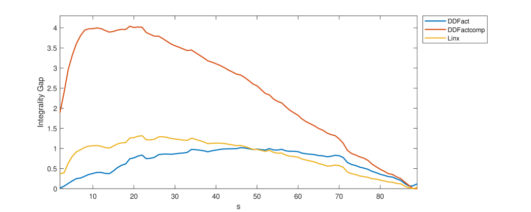
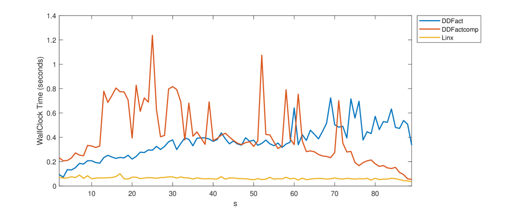
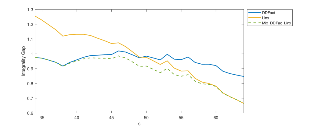
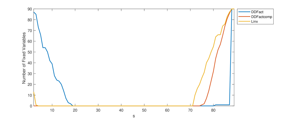
Figure 2: Bounds/times comparison and effect of the mixing and variable-fixing methodologies for $n=90$

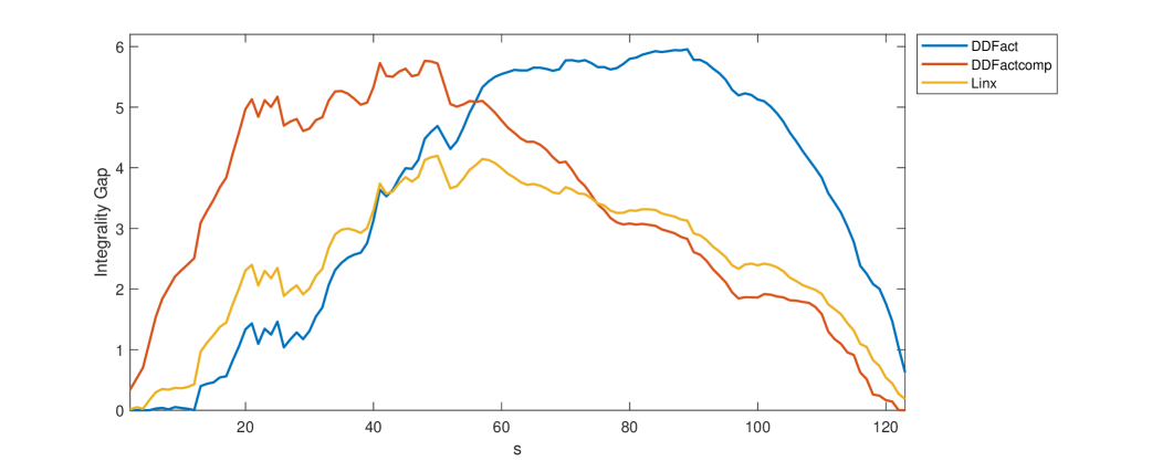
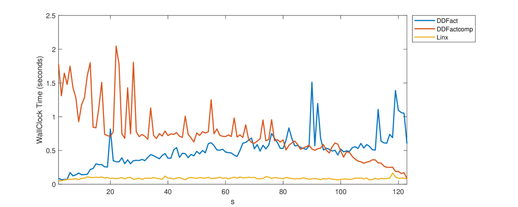
xxx

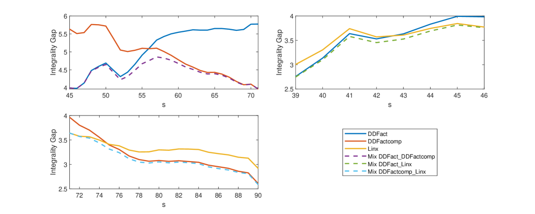
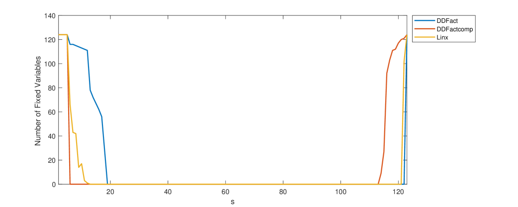
Figure 3: Bounds/times comparison and effect of the mixing and variable-fixing methodologies for $n=124$

For the three nonsingular covariance matrices used in our experiments, we solved 2.4, 2.3 and complementary 2.3, for all $2\leq s\leq n-1$. For each matrix, we present four plots. In the first plots of Figures 1, 2 and 3, we present the integrality gap for each bound and each $s$. Each such gap is given by the difference between the upper bound computed by solving the relaxation and a lower bound obtained using a heuristic of (Lee 1998, Sec. 4) followed by a simple local search (see (Ko, Lee, and Queyranne 1995, Sec. 4)).

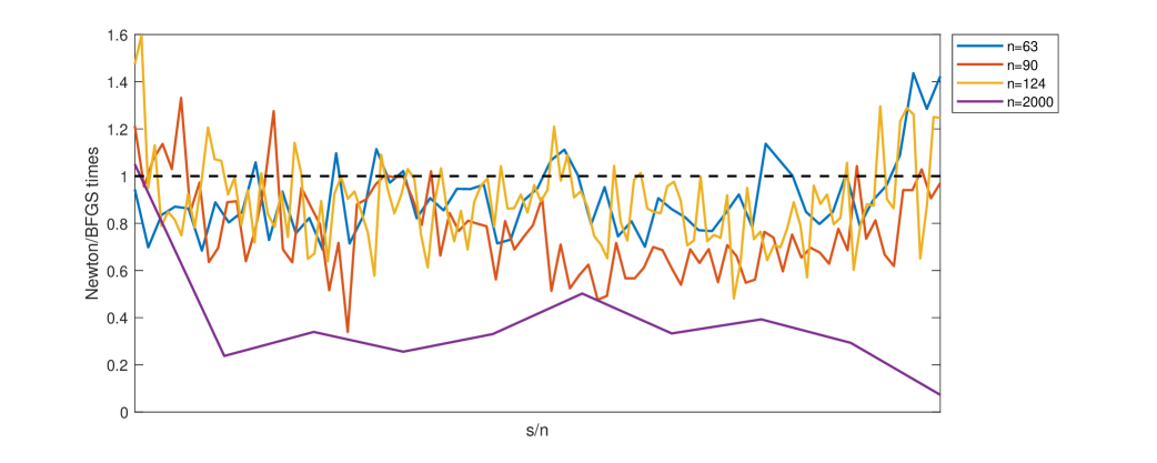
Figure 7: Newton/BFGS time for 2.4

In the second plots of those figures, we present the average wall-clock times (in seconds) used by Knitro to solve the relaxations. Some observations about the times presented are important. First, we note that the times depicted on the plots correspond to the application of a BFGS-based algorithm to solve 2.3 and complementary 2.3, and to the application of a Newton-based algorithm to solve 2.4. As an experiment, we also applied a BFGS-based algorithm to solve 2.4, not passing the Hessian to the solver, but, as expected, the results were worse concerning both time and convergence of the algorithm. The difference between the times can be seen in Table 6 (aggregated over $s$) and Figure 7. On the other hand, we did not apply a Newton-based algorithm to 2.3 and complementary 2.3 because we cannot guarantee that the objective function of these relaxations is differentiable at every iterate (of the nonlinear-programming solver). We should also note that the times shown in the plots for 2.4 do not include the times to compute the value of the parameter $\gamma$ in the problem formulation. This parameter value has a great impact on the 2.4 bound. We present the times to compute them, aggregated over $s$, in Table 6. Finally, we should mention that Knitro did not prove optimality for several instances solved. However, we could confirm the optimality of all solutions returned by Knitro, up to the optimality tolerance considered, by constructing a dual solution with duality gap less than the tolerance, with respect to the primal solution obtained by Knitro. To construct the dual solutions, we solved various special cases of the linear program $G(\hat{\Theta}_{1},\ldots,\hat{\Theta}_{m})$ (see §2.5). For 2.3, the construction uses (2), where we took $\epsilon=0$, which gives us a dual solution that is feasible within numerical accuracy.

On our experiments with instances of MESP (i.e., no side constraints), these linear programs have closed-form solutions and the times to compute them are not significant.

In the third plots of Figures 1, 2 and 3, we demonstrate the capacity of the mixing methodology described in §2.5 to decrease the integrality gap. As observed in Chen, Fampa, Lambert, and Lee (2021), the methodology is particularly effective when considering in mix, a weighted sum of the objective functions of two relaxations, such that the bounds obtained by each relaxation are close to each other. We exploit this observation in our experiments. For each covariance matrix, we select one or more pairs of relaxations for which the integrality-gap curves (presented in the first plots of the figures) cross each other at some point. Then, we mix these two relaxations and compute new mixed bounds for all values of $s$ in a promising interval, approximately centered at the point where the two curves cross. To select the parameter $\alpha$ that weights the objective in mix, we simply apply a bisection algorithm.

Finally, in the fourth plots of Figures 1, 2, and 3, we demonstrate how effective the strategy described in Theorems 2.7 and 2.11 can be to fix variables (e.g., the context could be fixing variables at the root node of the enumeration tree in applying a branch-and-bound algorithm). In all of our experiments, we use a fixing threshold of $10^{-10}$ which can be considered as rather safe in the context of the accuracy that we use to compute the relevant quantities. Although the mixing strategy can decrease the integrality gap for some instances, in our experiments this improvement is not enough to allow more variables to be fixed. Therefore, we do not consider the mixed bounds in these plots.

3.4 Analysis of the results for $n=63,90,124$

The analysis of the plots for the $n=63$ and $n=90$ covariance matrices are very similar to each other and are summarized in the following.

• We see from the first plots of Figures 1 and 2 that the complementary 2.3 bound is not competitive with the 2.3 and 2.4 bounds for these instances. For most values of $s$ the first bound is much worse than the two others. The complementary 2.3 bound is only a bit better than the 2.3 bound for very large values of $s$ and it is never better than the 2.4 bound. The integrality-gap curves for 2.3 and 2.4 cross at points close to an intermediate value of $s$. For smaller $s$, 2.3 gives the best bound and for larger $s$, 2.4 is the winner.

• Concerning the wall-clock time to compute the bounds, we see again a big disadvantage of complementary 2.3 in the second plots of Figures 1 and 2. Although it is faster than 2.3 on some instances with large $s$, we see that on most instances its time is much longer than the times for the two other relaxations, and with the greatest variability among the different values of $s$. The solution of 2.4 is always significantly faster than the solution of the two other relaxations for these instances. Finally, we note that the variation in the time to solve 2.4 for all values of $s$ is less than $1\%$, while there is a great variability for the other two relaxations.

• We see in the first plots of Figures 1 and 2 that the curves corresponding to 2.3 and 2.4 cross at points close to intermediate values of $s$, indicating a promising interval of values to mix these relaxations for both $n=63$ and $n=90$. Considering such intervals, we see in the third plots of Figures 1 and 2, how mixing 2.3 and 2.4 can in fact, decrease the integrality gap for some instances, being mostly effective for the values of $s$ for which the 2.3 bound and the 2.4 bound are very close to each other.

• In the fourth plots of Figures 1 and 2 we verify the increasing capacity to fix variables as the bound gets stronger. Interestingly, we see that for large values of $s$, complementary 2.3 bounds can lead to more variables fixed than the better 2.3 bound.

For $n=124$, we have a slightly different analysis because, as we see in the first plot of Figure 3, the complementary 2.3 bound becomes better than the 2.3 bound for all $s$ larger than an intermediate value. We note that we can observe this same behavior with the “NLP” relaxation for CMESP used in Anstreicher, Fampa, Lee, and Williams (1999). Moreover, we see in the first plot of Figure 3, two points where the curves cross, showing three interesting intervals for $s$, where each one of the three relaxations gives the best bound. Concerning the wall-clock time, the observations about the second plot of Figure 3 are similar to the ones about the second plots of Figures 1 and 2, confirming that the time to solve 2.4 is shorter and with a smaller variability with $s$, when compared to the two other relaxations. In the third plot of Figure 3, we exploit the three crossing points of the integrality-gap curves for $n=124$, and show separately the capacity of the mixing methodology to decrease the gaps when we mix the two relaxations corresponding to each crossing point. It is interesting to note that the mixing methodology is more effective when the crossing curves are less flat at those points, that is, when the gaps change faster as $s$ changes. Finally, we have different observations about the fourth plot of Figure 3 when compared to the smaller instances, concerning the capacity of the relaxations to fix variables. As 2.3 and complementary 2.3 lead to very small integrality gaps at both ends of the curves, we observe in the fourth plot of Figure 3 their stronger capacity of fixing variables on the corresponding values of $s$, when compared to 2.4. For $n=124$, we see that 2.4 gives the best bounds for intermediate values of $s$ only. These are clearly the most difficult instances for $n=124$. Therefore, the integrality gap is usually not small enough on these instances to allow variable fixing.

3.5 Numerical experiments with the large instance ($n=2000$)

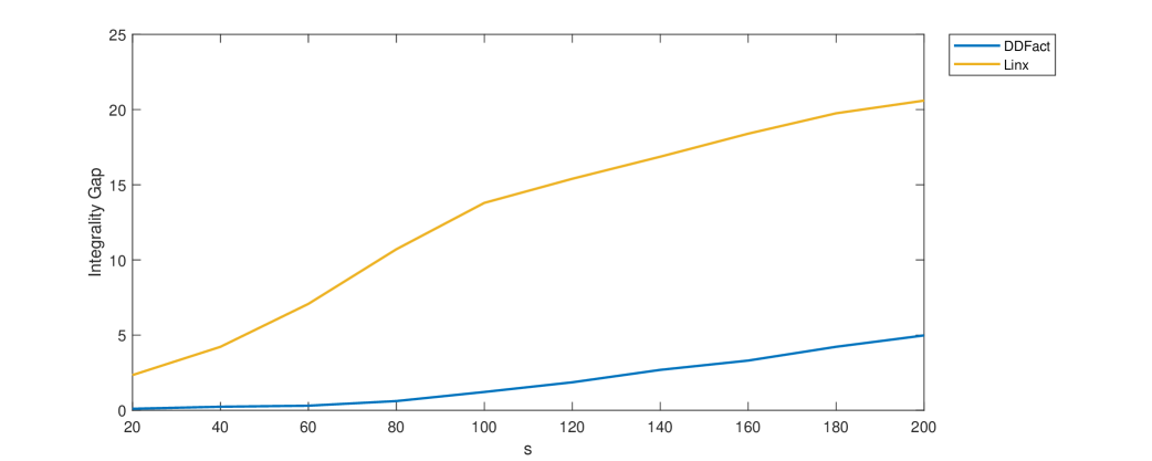
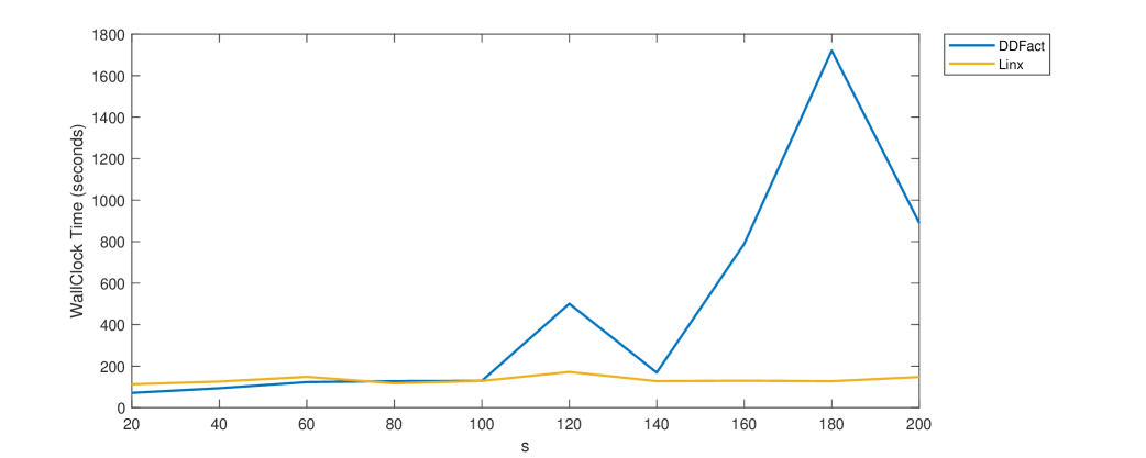
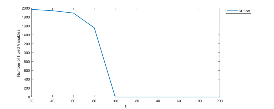
Figure 4: Bounds/times comparison and effect of the variable-fixing methodology for $n=2000$

The bounds computed for the $n=2000$ matrix are analyzed in Figure 4. As this larger matrix is singular, we could not apply the complementary 2.3 relaxation to obtain a bound. In the first plot, we present the integrality gaps for 2.3 and 2.4 for all $20\leq s\leq 200$ that are multiples of 20. For lower bounds in computing the gaps, we obtained them by the same heuristic applied to our smaller instances with $n=63,90,124$. We clearly see the superiority of 2.3 for this input matrix, for these relatively small values of $s$, following the behavior observed for the smaller instances. Concerning the wall-clock time, we still see in the second plot that 2.4 can be solved faster on the most difficult instances with $s\geq 100$, and once more, we see a very small variability in the times for 2.4, unlike what we see for 2.3. The significant rank deficiency of the covariance matrix of these instances would seem to be a disadvantage for 2.4 relative to 2.3, with regard to the computational time needed to solve them; this is because the order of the matrix considered in the objective function of 2.4 is always equal to the order of the covariance matrix, while for 2.3 it is given by its rank. As 2.4 could not fix variables for any value of $s$, we present in the third plot only the number of variables fixed for each $s$, considering the 2.3 bound, and we can see that the fixing procedure is very effective when $s\leq 80$ .

Our success with fixing using the 2.3 bound on the $n=2000$ matrix, for $s=20,40,60,80$, gave us some hope to solve these instances to optimality, or at least reduce them to a size where we could realistically hope that branch-and-bound could succeed. So we devised an iterative fixing scheme, applying fixing to a sequence of reduced instances, with the goal of solving to optimality or at least fixing substantially more variables. At each iteration, we calculated and attempted to fix based on the 2.3 bound and the 2.4 bound. We re-applied the heuristic for a reduced problem, in case it could improve on the lower bound of its parent. Even though the 2.4 bound cannot fix any variables at the first iteration, for $s=20,40,60$, it enabled us to fix more variables for reduced problems. For $s=20,40,60$, we could solve to optimality. The results are summarized in Table 5, where $s^{\prime}$ and $n^{\prime}$ are the parameters for reduced problems, by iteration, and $*$ indicates the iteration where we can assert that fixing identified the optimal solution. Unfortunately, for $s=80$, 2.4 could not fix anything after one round of 2.3 fixing. We noted that for $s=20,40,60$, the heuristic applied to the $n=2000$ root instance gave what turned out to be the optimal solution. It is possible that we did not succeed on $s=80$ because our lower bound is not strong enough.

We carried out some additional experiments for the $n=2000$ matrix, with $s=860,880,\ldots,940$ (recall that the rank of $C$ is 949). For these instances, 2.3 is very hard for Knitro to solve: the solution times for 2.3 are an order of magnitude larger as compared to the instances with $20\leq s\leq 200$; this is not the case for 2.4. Additionally, Knitro failed to converge for $s=920$. In any case, for all of these problems that we could solve, we had huge integrality gaps, and no variables could be fixed based on either 2.4 or 2.3.

3.6 More specifics about the computational time

In Table 6, we show means and standard deviations of the average wall-clock times (in seconds) for the main procedures considered in our experiments and for each $n$. For $n=63,90,124$, the statistics consider the solution for all $2\leq s\leq n-1$. For $n=2000$, the statistics consider all $20\leq s\leq 200$ that are multiples of 20.

In Table 6, the columns “DDFact”, “DDFactcomp” and “linx (Newton)” summarize information depicted in the second plots of Figures 1, 2, and 3. For each $n$, the mean and standard deviation of the times increase in the order: 2.4, 2.3, complementary 2.3, and the means and standard deviations are all significantly better for 2.4.

In Table 6, the column “linx (BFGS)” presents the mean and standard deviation of the times (across all $s$) when 2.4 is solved by Knitro without passing the Hessian of the objective function to the solver, i.e., with the application of a BFGS-based algorithm. We see that not passing the Hessian of the objective function to the solver leads to a significant increase in the solution time, and also in the variability of the times across the different values of $s$. Although we can see performance aggregated over $s$ in the “linx (Newton)” and “linx (BFGS)” columns, in Figure 7, we get a more complete view of the strong dominance, across most $s$ for each input matrix $C$. We have plotted the time for linx (Newton) divided by time for linx (BFGS), against $s/n$. With the vast majority of the ratios being less than one for each input matrix, and this emphatically being the case for the $n=2000$ matrix, we can confidently recommend passing the Hessian to Knitro when solving 2.4.

In Table 6, the column “$\gamma$ (Newton)” in Table 6 presents statistics for the time used to compute the value of the parameter $\gamma$ used in 2.4 across the different $s$. To optimize $\gamma$ we do a one-dimensional search, exploiting the fact that the 2.4 bound is convex in the logarithm of $\gamma$ (see Chen, Fampa, Lambert, and Lee (2021)), and we use Knitro passing the Hessian at each iteration of the one-dimensional search. We observe that, compared to solving 2.4, optimizing $\gamma$ is very expensive, however, we should note that the optimization procedure applied had no concern with time. When time is relevant, as in the context of a branch-and-bound algorithm, we can apply a faster procedure, like the one applied in Anstreicher (2020). Furthermore, we should notice that in a branch-and-bound context, the 2.4 bound is computed for each subproblem considered, but the parameter $\gamma$ should not be optimized for every one of them. As done in Anstreicher (2020), it would be more efficient to use the same parameter value as the one used on the parent node most of the times.

3.7 Some experiments with CMESP

To illustrate the application of our bounds to CMESP, we repeated the experiments performed with the instances of MESP with covariance matrix of dimension $n=63$ and $5\leq s\leq 47$, but now including five side constraints $a_{i}^{\top}x\leq b_{i}$, for $i=1,\ldots,5$. The left-hand side of constraint $i$ is given by a uniformly-distributed random vector $a_{i}$ with integer components between $1$ and $5$. The right-hand side of the constraints was selected so that, for every $5\leq s\leq 47$, the best known solution $x^{*}(s)$ of the instance of MESP is violated by at least one constraint. For that, each $b_{i}$ was selected as the $80$-th percentile of the values $a_{i}^{\top}x^{*}(s)-1$, for all $5\leq s\leq 47$. We note that when considering side constraints, the linear program $G(\hat{\Theta}_{1},\ldots,\hat{\Theta}_{m})$ does not have a closed-form solution. In this case, we solve it with Knitro. The time needed to calculate the dual solution with the Knitro linear-programming solver is no more than $5\%$ of the time needed to calculate the 2.3 bound or the complementary 2.3 bound. However, for the 2.4 bound, the variability of the times is large; for some instances, the time needed to construct the dual solution can even exceed the time needed to calculate the 2.4 bound.

In Figure 8 we present plots for CMESP, analogous to those shown in Figure 1 for MESP, considering our instances of dimension $n=63$. We have a very similar analysis of the results presented in both figures, illustrating the robustness of our approach when including side constraints to MESP.

4 Discussion

We developed some useful properties of the 2.3 bound, aimed at guiding computational practice. In particular, we saw that (i) the 2.3 bound is invariant under the chosen factorization of the input matrix $C$, (ii) the 2.3 bound cannot be improved by scaling $C$, and (iii) the 2.3 bound dominates the spectral bound. We developed a fixing scheme for 2.3, we demonstrated how to mix 2.3 with 2.4 and with complementary 2.3 (see (Chen, Fampa, Lambert, and Lee 2021, Sec. 7)) for general comments on how and when mixing could potentially be employed within branch-and-bound), and we gave a general variable-fixing scheme for these mixings.

Overall, we found that working with a general-purpose nonlinear-programming solver is quite practical for solving 2.4 and 2.3 relaxations of CMESP. For 2.3, this is despite the fact that its objective function is not guaranteed to be smooth at all iterates (of the nonlinear-programming solver). We found that for 2.4, which has a smooth objective function, passing the Hessian to the nonlinear-programming solver is quite effective; the running times are much better, in mean and variance, compared to a BFGS-based approach. We found that various mixings of 2.4, 2.3 and complementary 2.3 can lead to improved bounds. We found that fixing can be quite effective for 2.3 and complementary 2.3. Unfortunately, we did not find mixing to be useful for fixing additional variables, as compared to fixing variables based on each relaxation separately, on the benchmark instances that we experimented with. But we did find iterative fixing, employing the 2.4 and 2.3 fixing rules in concert, to be quite effective on large and difficult instances; for the $n=2000$ matrix and $s=20,40,60$, we could find and verify optimal solutions for the first time, and without any branching.

In future work, we plan to develop a full branch-and-bound implementation aimed at solving difficult instances of CMESP to optimality. Our experiments on benchmark covariance matrices indicate that such an approach should use both the 2.4 and 2.3 bounds. In particular 2.4 often seems to be valuable for the large values of $s$ (where 2.3 deteriorates). We can hope that variable fixing can be exploited for subproblems, and we expect that mixing is likely to be most valuable for subproblems that have $s$ near the middle of the range.

Additionally, we plan on working further on improving the algorithmics for the 2.3 relaxation, for modern settings in which the order $n$ of the covariance matrix greatly exceeds its rank $r$. Specifically: (i) we plan to take better advantage of the fact that the matrix in the objective function of 2.3 is order $r$ while in 2.4 it is order $n$; (ii) while the objective function of 2.3 is not guaranteed to be smooth at all iterates, we found that it usually is, and so we plan to use second-order information to improve convergence.

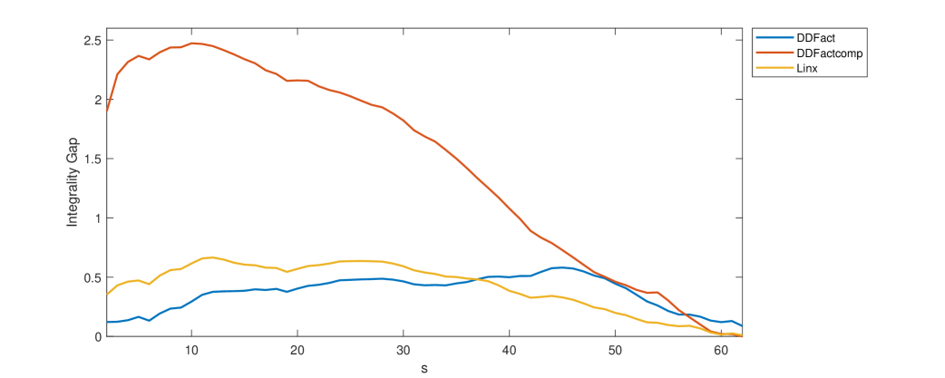
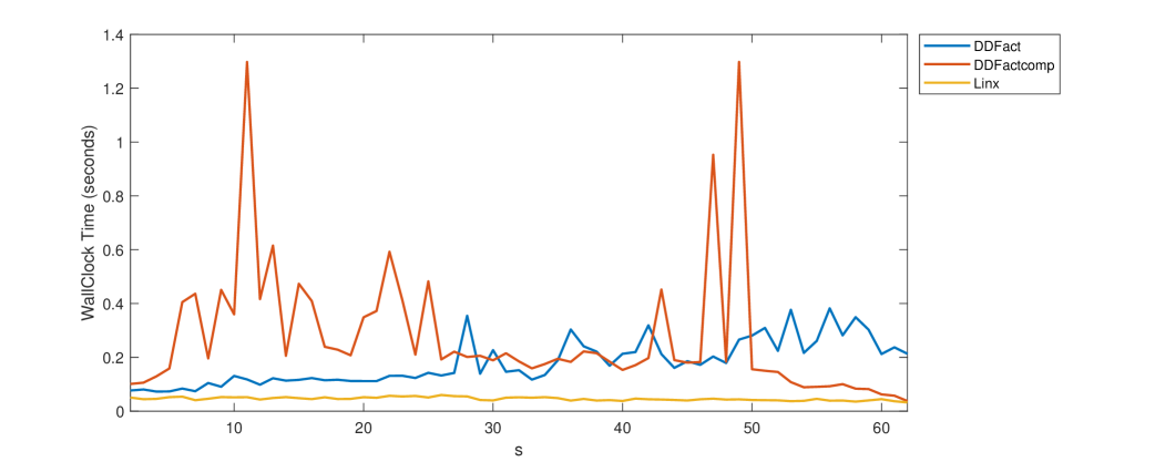
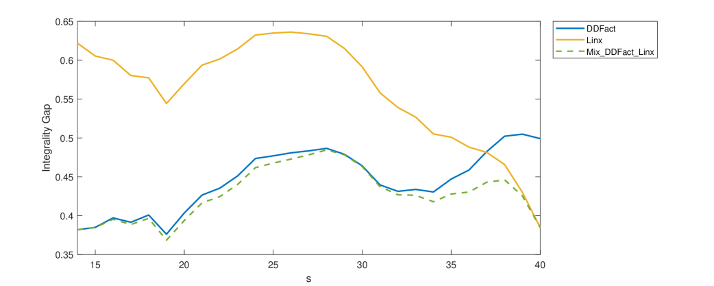
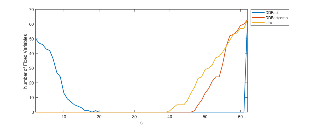
Figure 1: Bounds/times comparison and effect of the mixing and variable-fixing methodologies for $n=63$

Iter	$s^{\prime}$	$n^{\prime}$	$s^{\prime}$	$n^{\prime}$	$s^{\prime}$	$n^{\prime}$	$s^{\prime}$	$n^{\prime}$
0	20	2000	40	2000	60	2000	80	2000
1	20	28	40	58	60	110	80	442
2	2	7	6	13	22	68
3	$*$	$*$	3	4	16	24
4			1	2	1	2
5			$*$	$*$	$*$	$*$

Table 5: Iterated fixing for $n=2000$

$n$	DDFact		DDFactcomp		linx (Newton)		linx (BFGS)		$\gamma$ (Newton)
	mean	std	mean	std	mean	std	mean	std	mean	std
63	0.1807	0.0828	0.2756	0.2496	0.0459	0.0061	0.0518	0.0092	0.4202	0.0832
90	0.3653	0.1327	0.4163	0.2398	0.0629	0.0094	0.0849	0.0202	0.6727	0.1376
124	0.5023	0.2373	0.7451	0.3892	0.0874	0.0142	0.1005	0.0177	1.3043	0.2675
2000	461.49	536.37	-	-	133.69	17.54	542.93	530.50	2242.90	645.37

Table 6: Wallclock time (sec)

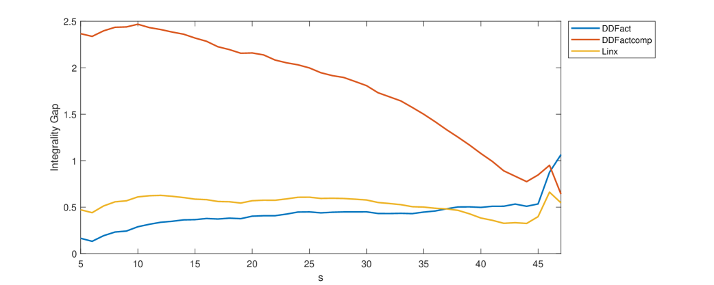
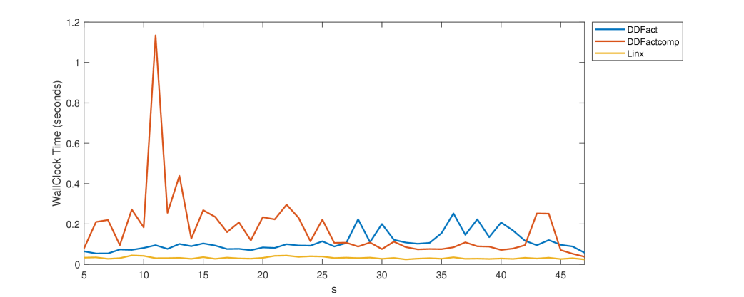
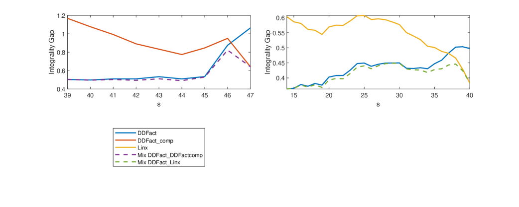
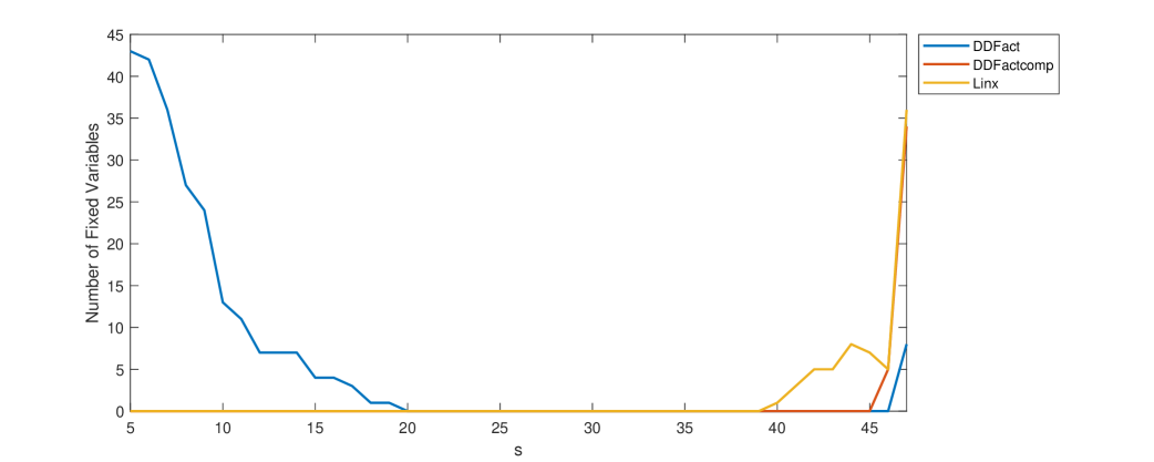
Figure 8: Bounds/times comparison and effect of the mixing and variable-fixing methodologies for $n=63$ with 5 side constraints (CMESP)

J. Lee was supported in part by AFOSR grant FA9550-19-1-0175. M. Fampa was supported in part by CNPq grants 305444/2019-0 and 434683/2018-3.

Lagrangian dual for mixing

The formulation mix can be recast as

$$\max\left\{\sum_{i=1}^{m}\alpha_{i}f_{i}(W_{i})~{}:~{}\mathbf{e}^{\top}x=s,~{}Ax\leq b,~{}0\leq x\leq\mathbf{e},~{}\alpha_{i}L_{i}(x)=\alpha_{i}W_{i},~{}i=1,\ldots,m~{}\right\}.$$

Next, we consider the Lagrangian function

$$\mathcal{L}(W_{1},\ldots,W_{m},x,\Theta_{1},\ldots,\Theta_{m},\upsilon,\nu,\pi,\tau):=$$

$$\quad\displaystyle\sum_{i=1}^{m}\alpha_{i}\Big{(}f_{i}(W_{i})+\Theta_{i}\bullet(L_{i}(x)-W_{i})\Big{)}+\upsilon^{\top}x+\nu^{\top}(\mathbf{e}-x)+\pi^{\top}(b-Ax)+\tau(s-\mathbf{e}^{\top}x),$$

with $\mbox{dom }\mathcal{L}=\left(\mathbb{S}^{k_{i}}_{+}\right)^{m}\!\times\!\mathbb{R}^{n}\!\times\!\left(\mathbb{S}^{k_{i}}\right)^{m}\!\times\!\mathbb{R}^{n}\!\times\!\mathbb{R}^{n}\!\times\!\mathbb{R}^{m}\!\times\!\mathbb{R}$. The corresponding dual function is

$$\mathcal{L}^{*}(\Theta_{1},\ldots,\Theta_{m},\upsilon,\nu,\pi,\tau):=\sup_{W_{i}\succeq 0,~{}x}\mathcal{L}(W_{1},\ldots,W_{m},x,\Theta_{1},\ldots,\Theta_{m},\upsilon,\nu,\pi,\tau),$$

and the Lagrangian dual problem is

$$\min\{\mathcal{L}^{*}(\Theta_{1},\ldots,\Theta_{m},\upsilon,\nu,\pi,\tau)~{}:~{}\upsilon\geq 0,~{}\nu\geq 0,~{}\pi\geq 0\}.$$

We note that

$$\sup_{W_{i}\succeq 0,~{}x}\mathcal{L}(W_{1},\ldots,W_{m},x,\Theta_{1},\ldots,\Theta_{m},\upsilon,\nu,\pi,\tau)=$$

$$\qquad\displaystyle\sum_{i=1}^{m}\alpha_{i}\sup_{W_{i}\succeq 0}\Big{(}f_{i}(W_{i})-\Theta_{i}\bullet W_{i}\Big{)}$$

$$\qquad\quad+\sup_{x}\left\{\displaystyle\sum_{i=1}^{m}\alpha_{i}\Big{(}\Theta_{i}\bullet L_{i}(x)\Big{)}+\upsilon^{\top}x+\nu^{\top}(\mathbf{e}-x)+\pi^{\top}(b-Ax)+\tau(s-\mathbf{e}^{\top}x)\right\}.$$

For $i=1,\ldots,m$, we assume that for any given $\hat{\Theta}_{i}\in\mathbb{S}^{k_{i}}_{++}$, there is a closed-form solution $\hat{W_{i}}$ to $\sup\{f_{i}(W_{i})-\hat{\Theta}_{i}\bullet W_{i}~{}:~{}W_{i}\succeq 0\}$, such that $\hat{\Theta}_{i}\bullet\hat{W}_{i}=:\rho_{i}\in\mathbb{R}$ and $\Omega_{i}:\mathbb{S}^{k_{i}}_{++}\rightarrow\mathbb{R}$, is defined by $\Omega_{i}(\hat{\Theta}_{i}):=f_{i}(\hat{W}_{i})$ and is convex. Furthermore, we assume that the supremum is $+\infty$ if $\Theta_{i}\nsucc 0$. Therefore

$$\displaystyle\alpha_{i}\sup_{W_{i}\succeq 0}\Big{(}f_{i}(W_{i})-\Theta_{i}\bullet W_{i}\Big{)}=\left\{\begin{array}[]{ll}\alpha_{i}\Big{(}\Omega_{i}(\Theta_{i})-\rho_{i}\Big{)},&\mbox{ if }\Theta_{i}\succ 0;\\ +\infty,&\mbox{ otherwise.}\end{array}\right.$$

We have

$$\sup_{x}\left\{\displaystyle\sum_{i=1}^{m}\alpha_{i}\Big{(}\Theta_{i}\bullet L_{i}(x)\Big{)}+\upsilon^{\top}x+\nu^{\top}(\mathbf{e}-x)+\pi^{\top}(b-Ax)+\tau(s-\mathbf{e}^{\top}x)\right\}$$

$$\quad\quad=\left\{\begin{array}[]{l}\displaystyle\sum_{i=1}^{m}\alpha_{i}\Big{(}\Theta_{i}\bullet L_{i0}\Big{)}+\nu^{\top}\mathbf{e}+\pi^{\top}b+\tau s,\\ \quad\quad\mbox{if}~{}\displaystyle\sum_{i=1}^{m}\alpha_{i}\Big{(}\Theta_{i}\bullet L_{ij}\Big{)}+\upsilon_{j}-\nu_{j}-\pi^{\top}A_{\cdot j}-\tau=0,~{}\mbox{ for }j\in N;\\ +\infty,\quad\mbox{otherwise.}\end{array}\right.$$

We see that the Lagrangian dual problem is equivalent to 2.5.

References

- Anstreicher (2018) Anstreicher KM (2018) Maximum-entropy sampling and the Boolean quadric polytope. Journal of Global Optimization 72(4):603–618.
- Anstreicher (2020) Anstreicher KM (2020) Efficient solution of maximum-entropy sampling problems. Operations Research 68(6):1826–1835.
- Anstreicher et al. (1996) Anstreicher KM, Fampa M, Lee J, Williams J (1996) Continuous relaxations for constrained maximum-entropy sampling. Integer programming and Combinatorial Optimization (Vancouver, BC, 1996), volume 1084 of Lecture Notes in Comput. Sci., 234–248 (Springer, Berlin).
- Anstreicher et al. (1999) Anstreicher KM, Fampa M, Lee J, Williams J (1999) Using continuous nonlinear relaxations to solve constrained maximum-entropy sampling problems. Mathematical Programming, Series A 85(2):221–240.
- Anstreicher et al. (2001) Anstreicher KM, Fampa M, Lee J, Williams J (2001) Maximum-entropy remote sampling. Discrete Applied Mathematics 108(3):211–226.
- Anstreicher and Lee (2004) Anstreicher KM, Lee J (2004) A masked spectral bound for maximum-entropy sampling. mODa 7—Advances in Model-Oriented Design and Analysis, 1–12, Contrib. Statist. (Physica, Heidelberg).
- Bagroy et al. (2017) Bagroy S, Kumaraguru P, De Choudhury M (2017) A social media based index of mental well-being in college campuses. Proceedings of the 2017 CHI Conference on Human Factors in Computing Systems, 1634–1646 (Association for Computing Machinery), https://doi.org/10.1145/3025453.3025909.
- Burer and Lee (2007) Burer S, Lee J (2007) Solving maximum-entropy sampling problems using factored masks. Mathematical Programming 109(2-3, Ser. B):263–281.
- Caselton et al. (1992) Caselton WF, Kan L, Zidek JV (1992) Quality data network designs based on entropy. Walden A, Guttorp P, eds., Statistics in the environmental and earth sciences, 10–38, London: Elsevier Science (London: Elsevier Science).
- Caselton and Zidek (1984) Caselton WF, Zidek JV (1984) Optimal monitoring network design. Statistics and Probability Letters 2:223–227.
- Chen et al. (2021) Chen Z, Fampa M, Lambert A, Lee J (2021) Mixing convex-optimization bounds for maximum-entropy sampling. Mathematical Programming, Series B 188:539–568.
- Dey et al. (2021) Dey SS, Mazumder R, Wang G (2021) Using -relaxation and integer programming to obtain dual bounds for sparse PCA. Operations Research (in press) .
- Fampa and Lee (2021) Fampa M, Lee J (2021) Maximum-entropy sampling: algorithms and application (Springer), in press.
- Frank and Wolfe (1956) Frank M, Wolfe P (1956) An algorithm for quadratic programming. Naval Research Logistics Quarterly 3(1–2):95–110.
- Guttorp et al. (1993) Guttorp P, Le ND, Sampson PD, Zidek JV (1993) Using entropy in the redesign of an environmental monitoring network. Patil G, Rao C, Ross N, eds., Multivariate Environmental Statistics, volume 6, 175–202 (North-Holland).
- Hoffman et al. (2001) Hoffman A, Lee J, Williams J (2001) New upper bounds for maximum-entropy sampling. mODa 6—Advances in Model-Oriented Design and Analysis (Puchberg/Schneeberg, 2001), 143–153, Contrib. Statist. (Physica, Heidelberg).
- Horn and Johnson (1985) Horn RA, Johnson CR (1985) Matrix Analysis (Cambridge University Press, Cambridge), First edition, ISBN 0-521-38632-2.
- Ko et al. (1995) Ko CW, Lee J, Queyranne M (1995) An exact algorithm for maximum entropy sampling. Operations Research 43(4):684–691.
- Lee (1998) Lee J (1998) Constrained maximum-entropy sampling. Operations Research 46(5):655–664.
- Lee (2012) Lee J (2012) Maximum entropy sampling. El-Shaarawi A, Piegorsch W, eds., Encyclopedia of Environmetrics, 2nd ed., 1570–1574 (Boston: Wiley).
- Lee and Williams (2003) Lee J, Williams J (2003) A linear integer programming bound for maximum-entropy sampling. Mathematical Programming, Series B 94(2–3):247–256.
- Li and Xie (2020) Li Y, Xie W (2020) Best principal submatrix selection for the maximum entropy sampling problem: scalable algorithms and performance guarantees. Preprint at: https://arxiv.org/abs/2001.08537.
- Löfberg (2004) Löfberg J (2004) Yalmip : A toolbox for modeling and optimization in Matlab. Proceedings of the CACSD Conference.
- Nikolov (2015) Nikolov A (2015) Randomized rounding for the largest simplex problem. Proc. of the 47th Annual ACM Symposium on Theory of Computing, 861–870, STOC ’15 (New York: ACM).
- Sebastiani and Wynn (2000) Sebastiani P, Wynn HP (2000) Maximum entropy sampling and optimal Bayesian experimental design. Journal of the Royal Statistical Society: Series B (Statistical Methodology) 62(1):145–157.
- Shewry and Wynn (1987) Shewry MC, Wynn HP (1987) Maximum entropy sampling. Journal of Applied Statistics 46:165–170.
- Toh et al. (1999) Toh KC, Todd MJ, Tütüncü RH (1999) SDPT3: A Matlab software package for semidefinite programming, version 1.3. Optimization Methods and Software 11(1-4):545–581.
- Tsing et al. (1994) Tsing NK, Fan MK, Verriest EI (1994) On analyticity of functions involving eigenvalues. Linear Algebra and its Applications 207:159 – 180.
- Wu and Zidek (1992) Wu S, Zidek JV (1992) An entropy-based analysis of data from selected nadp/ntn network sites for 1983–1986. Atmospheric Environment. Part A. General Topics 26(11):2089 – 2103.
- Zidek et al. (2000) Zidek JV, Sun W, Le ND (2000) Designing and integrating composite networks for monitoring multivariate Gaussian pollution fields. Journal of the Royal Statistical Society. Series C. Applied Statistics 49(1):63–79.