A Bayesian network model for predicting cardiovascular risk

Abstract

We propose a Bayesian network model to make inferences and predictions about cardiovascular risk. Both the structure and the probability tables in the underlying model are built using a large dataset collected in Spain from annual work health assessments, with uncertainty characterized through posterior distributions. We illustrate its use for public health practice, policy and research purposes. A freely available version of the software is included in an Appendix.

[inst1]organization=Nutrition and Genomics, JM-USDA-HNRCA, Tufts University,city=Boston, state=MASS, country=USA

[inst2]organization=ICMAT-CSIC,city=Madrid, country=Spain [inst3]organization=i+Health, Dpt. Health Sciences, European University Miguel de Cervantes,city=Valladolid, country=Spain [inst4]organization=Physical Activity and Health Research Group, Inst. Inv. Sanitaria Hospital 12 de Octubre,city=Madrid, country=Spain [inst5]organization=Fac. Sports Sciences, Universidad Europea de Madrid,city=Madrid, country=Spain [inst6]organization=Inst. de Mathématiques Apliqueés, Université Catholique de L’Ouest,city=Angers, country=France

1 Introduction

Cardiovascular diseases (CVD) are the leading cause of mortality in Europe and are responsible for over 3.9 million deaths per year (45% of all deaths). Additionally, the yearly costs for CVD treatment surpass 210 billion euros in Europe (1).

Prediction scores are important tools for the prevention and management of CVD. In the clinical setting, accurate individual prediction of CVD risk is highly desirable to support the screening of high-risk patients, guide clinicians to determine and develop appropriate intervention strategies, and increase patient adherence.

CVD epidemiology can be traced back to the 1930s, with early studies describing an increased prevalence of CVD-related mortality with industrialization and affluence. The still ongoing Framingham Heart Study was founded in 1948 to examine the epidemiology of CVD and has provided a wealth of information on CVD risk factors (CVRFs) (2). Such factors are defined as measurable characteristics associated with increased disease frequency and are viewed as significant independent predictors of an increased risk of presenting such disease. The World Health Organization (WHO) has established a set of modifiable and non-modifiable CVRFs, which mainly address myocardial infarction (heart attack) and stroke (3). Non-modifiable factors are those over which individuals have no control, including genetics, age, sex, and ethnicity. By contrast, modifiable CVRFs comprise behavioral factors that may evolve with individual activity, including physical activity (PA), diet, alcohol, and tobacco consumption. The list of modifiable CVRFs is complemented by health indicators directly influenced by individuals’ behavior, including body mass index, blood pressure, and lipidemia, among others. It is worth noting that the list of CVRFs established by the WHO is subject to frequent revision and validation (4; 1).

Interest in Bayesian networks (BNs) (5) in the healthcare community has increased over the last two decades (6), (7), (8). Their ability to consistently and systematically integrate large amounts of data makes them well-suited to quantify the conditional probability tables that BNs require. In particular, for CVD diagnosis and prognosis, BNs represent a natural set-up for analyzing dependence across variables concerning related risk factors for CVD. For instance, (9) developed a BN for coronary angiography risk assessment. Some years later, (10) proposed a BN to perform real-time CVD diagnosis focusing on myocardial infarction, infective endocarditis and hyperpotassemia. (11) built a simple BN model of the CV system and evaluated its ability to predict unobservable variables regarding the internal patient state. In relation to CVD epidemiology, one of the earliest studies constructing a BN linking various CVRFs to estimate CVD risk was performed by (12). Later, (13) constructed an epidemiological CVD BN using data collected on individuals free of CVD, with the purpose of following-up patients over two years and assessing CVD events. Likewise, (14) proposed a discrete BN to identify and analyze the relationships among thirteen epidemiological features in the heart domain.

The purpose of the present study was to analyze relationships between several well-established CVRFs and additional factors that may contribute to CVD, focusing on the positive impact of PA (see (15; 16) for earlier insights into the relevance of PA for CVD). To achieve this objective, we used a discrete BN, with each node representing a CVRF or a medical condition. Both the BN structure and its probability tables are learnt from a large dataset originating from annual health assessments. Importantly, we characterize the uncertainty about such probabilities through (higher-order) distributions. While the typical objective in the aforementioned literature is the analysis of CVD risk scores, here we emphasize the predictive assessment of various CVRFs and further integrate additional factors such as depression, sleep duration or socioeconomic status, and analyze them through a BN-based framework. One of the main advantages of our model is that it allows assessing predictions for each factor, or sets of factors, using probabilistic inference. This can be used as a complementary decision-support tool to facilitate diagnosis and treatment by allowing practitioners to better foresee patients’ conditions. Moreover, it can also serve as a validating tool to check how likely the patient’s condition could have been forecast by the model based on past data.

The paper is structured as follows: Section 2 describes the dataset used to structure and calibrate the BN; in section  3, we formulate the BN model describing the structure learning process as well as the marginal distribution for each node; section 4 presents several uses of the model; and, finally, section 5 summarizes and discusses our findings. An appendix briefly describes a freely available software to perform predictions based on our proposed BN.

2 Data set

Data were extracted from the annual work health assessments of adult workers affiliated with a private insurance provider in Spain, from 2012 to 2016 and were anonymized and secured. Data were complemented with census information based on postal code, allowing us to infer the associated socioeconomic status (combining occupation, economic activity and professional situation averaged across the entire postal code) and education level (level 0 to 4, where 0 represents illiterate people and 4 represents people with a university degree or higher). We removed outliers, duplicates, misrecorded and missing values, and retained only the last assessment available for each individual leading to a total of 205,087 health assessments over the 4-year period.

The variables relevant in this study are listed in Table 1 and are grouped as follows:

• Non-modifiable CVRFs: sex, age, education, and socioeconomic status.

• Modifiable CVRFs: body mass index (BMI), PA, sleep duration, smoking profile, anxiety, and depression.

• Medical conditions: hypertension, hypercholesterolemia, and diabetes.

Table 1 provides the values of the variables.

Variable	Definition	Levels
$v_{1}$	Sex	{female, male}
$v_{2}$	Age	{[18-24], (24-34], (34-44],
		(44-54], (54-64], (64-74]}
$v_{3}$	Education level	{1,2,3}
$v_{4}$	Socioeconomic status	{1,2,3}
$v_{5}$	Body mass index	{underw., normal, overw., obese}
$v_{6}$	Physical activity	{ insufficiently active (1), regularly active (2) }
$v_{7}$	Sleep duration	{ Short; Normal; Excessive}
$v_{8}$	Smoker profile	{non-smoker, ex-smoker, smoker}
$v_{9}$	Anxiety	{yes, no}
$v_{10}$	Depression	{yes, no}
$v_{11}$	Hypertension	{yes, no}
$v_{12}$	Hypercholesterolemia	{yes, no}
$v_{13}$	Diabetes	{yes, no}

Table 1: Variables in model

Age was categorized into six age groups following the grouping of the Spanish National Statistical Institute in their National Sport Habits survey, as in (15): (18-24), (24-34), (34-44), (44-54), (54-64) and (64-74). Education and socioeconomic levels were discretized to 1, 2, 3 (larger indices for higher education or socioeconomic levels).

As for modifiable CVRFs, we followed the WHO BMI guidelines for underweight (<18.5 kg/m²), normal weight (18.5-25 kg/m²), overweight (25-29.9 kg/m²), and obese ( $\geq$ 30 kg/m²) classes. Participants’ self-reported leisure-time PA levels were assessed as in (16), allowing the categorization of insufficiently active (not meeting WHO minimum recommendations for aerobic PA in adults, i.e., <150min/wk and <75min/wk in moderate and vigorous PA, respectively), or regularly active (meeting WHO guidelines). Sleep duration was categorized as short (less than 6 hours), normal (6-9 hours) and excessive (> 9 hours). The smoker profile indicated whether the patient was currently an active smoker, had never smoked or was an active smoker in the past. Finally, we extracted from the data whether the patient had been clinically diagnosed with anxiety and depression.

With regard to medical conditions, in addition to previous medical history, we also determined whether patients had diabetes (i.e., medicated or glycaemia $\geq 125$ mg/dL), hypercholesterolemia (medicated or total cholesterol $\geq 240$ mg/dL), or hypertension (medicated or systolic/diastolic blood pressure $\geq 140$/$90$mm Hg).

Table 2 lists the proportion of cases in various categories reflecting, by and large, the standard structure of the Spanish labor force (with the exception of the lower presence of females and of more senior people in our study than in the overall labor market due to the types of companies served by the insurance provider) and its health status. In particular, we found a high proportion of (i) overweight to obese subjects; (ii) smokers; (iii) hypertensive and hypercholesterolemic individuals; and (iv) a high proportion of subjects not meeting the WHO-recommended PA levels. By contrast, anxiety, diabetes and depression were at relatively low levels.

Variables	States	Marginal		Variables	States	Marginal
BMI	Underweight	1.16%		Diabetes	Yes	2.51%
	Normal	40.74%			No	97.49%
	Overweight	40.31%		Hypertension	Yes	15.05%
	Obese	17.79%			No	84.95%
Sex	Female	32.10%		Hypercholest.	Yes	30.53%
	Male	67.90%			No	69.47%
Smoker	Non-Smoker	50.14%		Physical Act.	1	75.63%
profile	Ex-Smoker	20.49%			2	24.37%
	Smoker	29.37%
Age(y)	(18-24)	0.71%		Educ. lev.	1	0.21%
	(24-34)	17.10 %			2	76.65%
	(34-44)	36.81%			3	23.14%
	(44-54]	30.37%		Sleep Dur.	< 6h	11.66%
	(54-64)	14.83%			(6h-9h)	88.25%
	(64-74)	0.18%			> 9h	0.09%
Socioeconomic	1	37.83%		Depression	No	99.52%
status	2	35.15%			Yes	0.48%
	3	27.02%
Anxiety	Yes	2.68%
	No	97.32%

Table 2: Percentage of observations at each class

We performed this exploratory analysis for each of the years as a sensitivity analysis, revealing relatively minor differences. This suggested stability of the workforce health structure over the five years available, allowing us to safely aggregate the data over that period.

3 A Bayesian network for cardiovascular risk factors

We built a discrete BN to estimate the joint distribution underlying the available data as the basis to make inferences and predictions on cases of relevance. The variables in the BN nodes were coded as in Table 1. We used a two-stage search-and-score procedure to learn the structure of the BN.

First, we employed greedy thick thinning (17), a Bayesian search algorithm to estimate the initial structure from the data, which is based on a conditional independence test that scores BN structures according to a conditional dependence measure. It is suitable when the amount of available data is large, as in our case, as it converges asymptotically to the eventual actual structure (18).

The second stage was an empirical iterative procedure involving several (three) experts in the CVD domain. The experts were shown various BN structures and asked to prune or add relevant edges reasoning on a cause-effect mechanism between “parent-children” sets of nodes. Various iterations were needed to agree on the final BN structure shown in Figure 1, with different colors for medical conditions (blue) and modifiable (white) and non-modifiable (pink) CVRFs. As a consequence of the graphical representation, the underlying suggested probabilistic model over the thirteen variables is

$$p(v_{1},\dots,v_{13}) =\Big{[}p(v_{1})p(v_{2})p(v_{3}|v_{1},v_{8})p(v_{4}|v_{1},v_{2},v_{3},v_{5},v_{6},v_{8})\Big{]}\times$$

$$\Big{[}p(v_{5}|v_{2},v_{6},v_{8})p(v_{6}|v_{1},v_{2},v_{7},v_{8})p(v_{7}|v_{2})p(v_{8}|v_{1},v_{2})$$

$$p(v_{9}|v_{1},v_{7},v_{10},v_{11})p(v_{10}|v_{1},v_{3})\Big{]}\times$$

$$\Big{[}p(v_{11}|v_{5},v_{6},v_{7})p(v_{12}|v_{1},v_{2},v_{3},v_{6},v_{7},v_{8})p(v_{13}|v_{1},v_{2},v_{6})\Big{]},$$

where we have marked the three blocks of variables considered.

Figure 1: Layout of the Bayesian network structure. White (modifiable cardiovascular risk factors); light pink (non-modifiable cardiovascular risk factors); light blue (medical conditions). Abbreviations: $Edu$, education level; $SeC$, socioeconomic status ; $BMI$, body mass index; $PA$, physical activity; $SD$, sleep duration; $Smok$, smoker profile; $HypCh$, hypercholesterolemia; $Diab$: diabetes.

After defining the structure, we assessed the probability tables at various nodes using standard multinomial-Dirichlet models with uniform priors (19). As an example, we provide the expected values of the distributions at node $v_{7}$, sleep duration, in Table 3. Of note, the last column in the table suggests that 19.64% of the population in this age group sleeps less than 6 hours and 80.33% sleeps between 6 and 9 hours.

Sleep Duration (h) /age(y)	18-24	24-34	34-44	44-54	54-64	64-74
$<6$	4.67	6.94	10.16	13.50	17.30	19.64
$6-9$	94.98	92.93	89.77	86.43	82.61	80.33
$>9$	0.35	0.13	0.07	0.07	0.09	0.03

Table 3: Probability table at node $v_{7}$. Probabilities as expected values of the corresponding posterior distributions are expressed as percentages.

The proportion of workers with low sleep hours seems to increase with age. As an example, we tested whether the proportion of low sleeping hours for the 64–74 age group (whose posterior distribution is $\beta e(79,353)$) is larger than that for the 18–24 age group (whose posterior distribution is $\beta e(59,1900)$), with Bayesian hypothesis testing methods (20). Our simulation showed that the probability for the first proportion being larger than the second is almost 100%, supporting the above statement. On the other hand, when comparing the proportions for the 64–74 and 54–64 age groups, the posterior probability was 75.7%. Henceforth, we will use the point estimates of the probabilities based on posterior expectations. The model has been cross-validated, displaying proper generalization with unseen data (21).

4 Treatment practices and policy uses

We now describe several treatment practices and policy uses of the graphical structure, exploiting the ability of BNs to makes inferences, issue forecasts and support decisions: information, measurements and observations can be inserted and propagated throughout the network and modify the distributions in other nodes based on probabilistic computations using Bayes’ formula (5), possibly applied several times. Accordingly, the network becomes a probabilistic database that summarizes the uncertainty about the CVD domain and may be queried to respond to diagnosis, treatment and policy issues.

4.1 Diagnosis and evidence propagation

First, we provide examples that combine inserted pieces of information to evaluate the predictive probability that a patient develops hypertension, a key point when dealing with CVD.

We first describe how such probabilities can be computed. These could refer to an individual with specific features for which we would forecast their likelihood of developing a particular medical condition, or to a group of individuals with such features for which we aim to predict the proportion of individuals that could develop such condition. For example, consider the scenario of a male aged over 44, sleeping less than 6 hours per night, overweight, sedentary, and having anxiety. The conditional probability that this person has hypertension, given the previous information, is described through

$$Pr(v_{11}=y\,|\,v_{1}=male,v_{2}\geq 45,v_{5}=overw.,v_{6}=1,v_{7}=\{<6h\}),v_{9}=y)=$$

$$\frac{Pr(v_{1}=male,v_{2}\geq 45,v_{5}=overw.,v_{6}=1,v_{7}=\{<6h\}),v_{9}=y,v_{11}=y)}{Pr(v_{1}=male,v_{2}\geq 45,v_{5}=overw.,v_{6}=1,v_{7}=\{<6h\}),v_{9}=y)}$$ (1)

Simple but computationally intensive, calculations based on the law of total probability would compute the probability of interest, which is 25.26%, well above the marginal probability (15.05%) of such an event shown in Table 2. This suggests an important increase in the probability of having hypertension for individuals with such a profile. In this case, had the individual not been diagnosed with such a medical condition, they should be notified about the elevated risk and the associated problems. Suppose now that the above calculations refer to a group with such features. Then, we would have identified a group in which to concentrate communication and intervention efforts, given the non-negligible increased probability of having the condition.

Table 4 lists other relevant examples, with a focus on the impact of PA. Specifically, using case (1) as a benchmark, we first consider the impact of PA (insufficiently active [1], regularly active [2]) in the first two lines: note the positive impact (more PA, smaller probability of developing hypertension) in such a group of patients. Next, using these two cases as a benchmark, we consider how sex affects the probabilities (the remaining features being the same) in the last column, two first rows; in both cases, women with such a health condition would tend to have a slightly greater probability of developing hypertension, although PA would still be beneficial.

Similarly, obesity (next two lines) entails a much higher risk of hypertension for both female and male workers than overweight at all PA levels, although PA still seems beneficial. Of course, when we consider the possibility that the person is overweight or obese (in addition to the other conditions), we obtain intermediate results, as shown in the last two rows.

BMI	Physical activity	Probability Male	Probability Female
Overw.	1	25.26	26.34
Overw.	2	19.79	20.70
Obese	1	45.54	46.95
Obese	2	34.49	35.78
Overw., obese	1	32.85	33.82
Overw., obese	2	22.90	23.85

Table 4: Probability of developing hypertension given various patient conditions for age greater than 44, poor sleeping level and anxiety.

4.2 Health research through hypothesizing evidence

We can also hypothesize evidence to address various types of health research issues. As an example, let us consider the impact of socioeconomic status on health conditions, as reflected in Table 5. The last column shows the prevalence of hypertension given the three socioeconomic levels: 14.65% (level 3), 14.90% (level 2) and 15.48% (level 1). This suggests a slightly increased prevalence of hypertension as the socioeconomic status decreases.

Status	Anxiety	Depression	Diabetes	Hypercholesterolemia	Hypertension
3	2.75	0.45	2.38	29.71	14.65
2	2.70	0.49	2.49	30.61	14.90
1	2.61	0.49	2.62	31.03	15.48

Table 5: Probability of health conditions given socio-economic status.

Similarly, we detect a slightly higher prevalence of hypercholesterolemia and diabetes with lower socioeconomic status. By contrast, higher socioeconomic status entails a slightly higher prevalence of anxiety. No effect is noted for depression.

Table 6 describes the BMI population structure depending on the socioeconomic status. For example, for the upper status 3, the structure is 1.18% for underweight, 42.53% for normal, 39.63% for overweight, and 16.66% for obese.

Status	Underweight	Normal	Overweight	Obese
3	1.18	42.53	39.63	16.66
2	1.22	41.54	40.09	17.15
1	1.10	38.70	41.01	19.19

Table 6: Probability of BMI population structure given socio-economic status.

Overall, Table 6 suggests a slightly worse BMI structure for the lower-income population.

4.3 Therapies through influential findings

Once we have determined a case of interest (group or individual) and assessed the relevant probability, we may wish to ascertain the influential findings over such statement. For this, we need only to eliminate the conditioning events one-by-one and determine the impact on the target probability, assessing the most influential finding based on the greatest reduction in probability. This is especially relevant in connection to modifiable CVRFs, for which we could explore the best modifications to suggest and communicate interventions to the individual or group by identifying those leading to the most significant reductions.

Consider a base case of a male individual aged 44–54 with education and socioeconomic status 3, who is obese, inactive, non-smoker, short sleep duration, and has anxiety but no depression. His probability of developing hypertension is 45.63%. Table 7 shows the probabilities when one of the included modifiable CVRFs is improved to its normal level and the others remain above normal. For example, the first row reflects that the probability of that individual having hypertension if we can improve his BMI level to normal is 11.30%.

MCVRF	Level	Probability
BMI	Normal	11.30
Physical activity	Regularly active	34.57
Sleep	Normal	39.69
Anxiety	No	37.02

Table 7: Probability of hypertension given improved conditions for a male aged 44-54, education and socioeconomic status 3, obese, low PA, insufficient sleep, with anxiety but no depression.

Consequently, it seems that the most effective intervention would be to recommend a diet to bring the BMI back to normal. Should we be able to improve the four conditions (i.e., reduce BMI, increase PA and sleep duration, while eliminating anxiety), the probability is reduced to 4.80%.

Note though, that, in order to elect the best recommendations, we would need to consider the possible impacts (e.g., costs, comfort, quality of life) of the medical conditions and treatments, possibly through a utility function and expected utility calculations (19).

5 Discussion

We have built a discrete BN that relates modifiable and non-modifiable CVRFs and relevant medical conditions and illustrated its use to forecast various conditions, support health research, determine relevant findings and facilitate treatment and policy choices. We have acknowledged uncertainty in the probability tables through posterior distributions.

Once the network is built (i.e., its structure and probability tables), implementing its computations is relatively straightforward using software like GeNIe or R. As an example, the appendix describes one version in GeNIe. Based on this, we could build a decision support system to facilitate clinical and policy decisions.

Two dynamic aspects not reflected in our model are relevant. First, additional data will be acquired annually by the insurance provider and the probability tables will be updated using Bayes’ formula. Second, we have aggregated the data over the years because of homogeneity, as described in Section 2; it would be interesting to develop a dynamic BN model to test for health status changes over time.

Finally, for more coherent decision support in choosing the best recommendation, we would need to consider the possible overall impact of the medical conditions and treatments using utility functions. In such cases, we would find the portfolio of recommendations with maximum expected utility.

Appendix: A GeNIe implementation of the model

A GeNIe version of the model (only for academic use) is available from https://github.com/jmcamachor1/CVD_GeNIe_network. Figure 2 displays the interface of the software, which requires prior downloading of GeNIe for proper functioning.

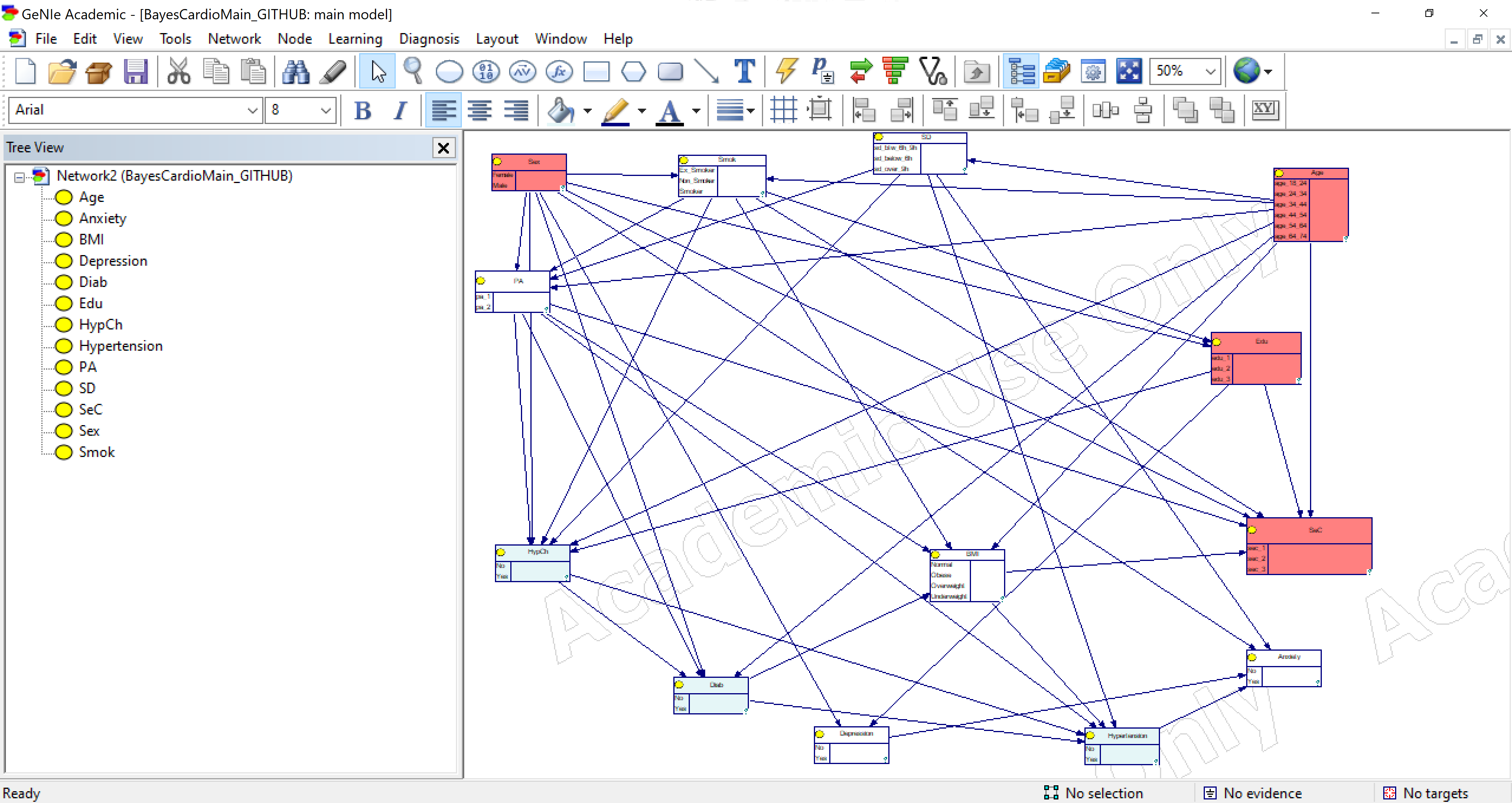
Figure 2: Interface of our model GeNIe implementation.

Based on it, we need only to use the GeNIe features to set evidence at nodes and declare other nodes as targets to find the required conditional probabilities. Clearing such evidence and targets reinitiates the original model and habilitates new probabilistic queries to the network. In such a way, we have robust interactive means to undertake research based on the proposed model.

Declaration of competing interest

We confirm that there are not conflict of interest associated with this publication.

Acknowledgements

Research supported by the AXA-ICMAT Chair in Adversarial Risk Analysis and the Spanish Ministry of Science program MTM2017-86875- C3-1-R. We are grateful to Quirónprevención for the provision of data. Research by A. Lucia is funded by the Spanish Ministry of Economy and Competitiveness and FEDER funds from the European Union (Grant P/18/00139). Discussions with Victoria Ley are gratefully acknowledged.

References

- (1) E. Wilkins, L. Wilson, K. Wickramasinghe, P. Bhatnagar, M. Rayner, N. Townsend, European Cardiovascular Disease Statistics, Tech. rep., European Heart Network (2017).
- (2) S. S. Mahmood, D. Levy, R. S. Vasan, T. J. Wang, The Framingham Heart Study and the epidemiology of cardiovascular disease: a historical perspective, The Lancet 383 (9921) (2014) 999–1008, https://doi.org/10.1016/S0140-6736(13)61752-3.
- (3) S. Kaptoge, al, World Health Organization cardiovascular disease risk charts: revised models to estimate risk in 21 global regions, The Lancet Global Health 7 (10) (2019) e1332–e1345, https://doi.org/10.1016/S2214-109X(19)30318-3.
- (4) E. Benjamin, et al., Heart Disease and Stroke statistics—2019 Update: A Report From the American Heart Association, Circulation 139 (10) (2019) e56–e528, https://doi.org/10.1161/CIR.0000000000000659.
- (5) T. Nielsen, F. Jensen, Bayesian Networks and Decision Graphs, Springer, New York, 2008.
- (6) E. Kyrimi, S. McLachlan, K. Dube, M. R. Neves, A. Fahmi, N. Fenton, A comprehensive scoping review of Bayesian networks in healthcare: Past, present and future, Artificial Intelligence in Medicine (2021) 102108https://doi.org/10.1016/j.artmed.2021.102108.
- (7) E. Kyrimi, K. Dube, N. Fenton, A. Fahmi, M. R. Neves, W. Marsh, S. McLachlan, Bayesian Networks in Healthcare: What is preventing their adoption?, Artificial Intelligence in Medicine (2021) 102079https://doi.org/10.1016/j.artmed.2021.102079.
- (8) S. McLachlan, K. Dube, G. A. Hitman, N. E. Fenton, E. Kyrimi, Bayesian networks in healthcare: Distribution by medical condition, Artificial Intelligence in Medicine 107 (2020) 101912, https://doi.org/10.1016/j.artmed.2020.101912.
- (9) K. Farooq, A. Hussain, S. Leslie, C. Eckl, C. MacRae, W. Slack, An Ontology Driven and Bayesian Network Based Cardiovascular Decision Support Framework, in: Advances in Brain Inspired Cognitive Systems, Springer Berlin Heidelberg, 2012, pp. 31–41, https://doi.org/10.1007/978-3-642-31561-9_4.
- (10) W. Tylman, T. Waszyrowski, A. Napieralski, M. Kamiński, T. Trafidło, Z. Kulesza, R. Kotas, P. Marciniak, R. Tomala, M. Wenerski, Real-time prediction of acute cardiovascular events using hardware-implemented Bayesian networks, Computers in Biology and Medicine 69 (2016) 245–253, https://doi.org/10.1016/j.compbiomed.2015.08.015.
- (11) J. M. Roberts, T. A. Parlikar, T. Heldt, G. C. Verghese, Bayesian Networks for Cardiovascular Monitoring, in: 2006 International Conference of the IEEE Engineering in Medicine and Biology Society, IEEE, 2006, pp. 205–209, https://doi.org/110.1109/IEMBS.2006.259985.
- (12) C. Twardy, A. Nicholson, K. Korb, J. Mcneil, Epidemiological data mining of cardiovascular Bayesian networks, Electronic Journal of Health Informatics 1 (2006) 1–13.
- (13) S. Thornley, R. J. Marshall, S. Wells, R. Jackson, Using Directed Acyclic Graphs for Investigating Causal Paths for Cardiovascular Disease, Journal of Biometrics & Biostatistics 04 (05) (2013) 1–6, https://doi.org/10.4172/2155-6180.1000182.
- (14) P. Fuster-Parra, P. Tauler, M. Bennasar-Veny, A. Ligęza, A. López-González, A. Aguiló, Bayesian network modeling: A case study of an epidemiologic system analysis of cardiovascular risk, Computer Methods and Programs in Biomedicine 126 (2016) 128–142, https://doi.org/10.1016/j.cmpb.2015.12.010.
- (15) P. Fernandez-Navarro, M. Aragones, V. Ley, Leisure-time physical activity and prevalence of non-communicable pathologies and prescription medication in Spain, PLoS ONE 1 (13) (2018) 1–13, https://doi.org/10.1371/journal.pone.0191542.
- (16) A. Santos-Lozano, A. T. Barrán, P. Fernández-Navarro, P. L. Valenzuela, A. Castillo-Garcia, L. M. Ruilope, D. R. Insua, J. M. Ordovas, V. Ley, A. Lucia, Association between physical activity and cardiovascular risk factors: Dose and sex matter, Journal of Sport and Health Science (2021) 604–606, https://doi.org/10.1016/j.jshs.2021.03.002.
- (17) J. Cheng, D. A. Bell, W. Liu, An Algorithm for Bayesian Belief Network Construction from Data, in: Proceedings of AI & STAT’97, 1997, pp. 83–90.
- (18) J. Pearl, Probabilistic Reasoning in Intelligent Systems, Morgan Kauffman Publishers, 1988.
- (19) S. French, D. Rios Insua, Statistical Decision Theory, Wiley, New York, 2000.
- (20) F. J. Giron, Bayesian Hypothesis Testing of Statistical Hypothesis, Real Academia de Ciencias, 2020.
- (21) R. Nagarajan, M. Scutari, S. Lèbre, Bayesian Networks in R: with Applications in Systems Biology, Springer, 2013.