Infinite energy maps and rigidity
Georgios Daskalopoulos
Department of Mathematics
daskal@math.brown.edu
and
Chikako Mese
Johns Hopkins University
cmese@math.jhu.edu
Abstract.
We extend Siu’s and Sampson’s celebrated rigidity results to non-compact domains. More precisely,
let M 𝑀 M M ~ ~ 𝑀 \tilde{M} X ~ ~ 𝑋 \tilde{X} g 𝑔 g p 𝑝 p 3 g − 3 + p > 0 3 𝑔 3 𝑝 0 3g-3+p>0 ρ : π 1 ( M ) → 𝖨𝗌𝗈𝗆 ( X ~ ) : 𝜌 → subscript 𝜋 1 𝑀 𝖨𝗌𝗈𝗆 ~ 𝑋 \rho:\pi_{1}(M)\rightarrow\mathsf{Isom}(\tilde{X}) ρ 𝜌 \rho u ~ : M ~ → X ~ : ~ 𝑢 → ~ 𝑀 ~ 𝑋 \tilde{u}:\tilde{M}\rightarrow\tilde{X} 𝗋𝖺𝗇𝗄 ( d u ~ ) ≥ 3 𝗋𝖺𝗇𝗄 𝑑 ~ 𝑢 3 \mathsf{rank}(d\tilde{u})\geq 3 u ~ ~ 𝑢 \tilde{u} [JZ ] and [M ] . We also extend these results to the case when the target is a Riemannian manifold with sectional curvature bounded from above by a negative constant.
GD supported in part by NSF DMS-2105226, CM supported in part by NSF DMS-2005406.
In his influential paper [Siu1 ] , Y.-T. Siu proved that harmonic maps between Kähler manifolds of complex dimension ≥ 2 absent 2 \geq 2 [Sa ] showed that a harmonic map from a compact Kähler manifold to a Riemannian manifold of nonpositive Hermitian sectional curvature is pluriharmonic. The compactness of the domain can be replaced by completeness and finite volume, provided that there exists a finite energy map (cf. [Siu2 ] and [Co1 ] ). However, in many situations, it may be difficult or even impossible to prove that a finite energy maps exists. The goal of this manuscript is to extend Siu’s and Sampson’s work by proving the existence of possibly infinite energy pluriharmonic or even holomorphic maps between Kähler manifolds.
Infinite energy harmonic maps between manifolds previously appeared the work of Lohkamp and Wolf. Lohcamp [Loh ] proved the existence of a harmonic map in a given homotopy class of maps between two non-compact manifolds, provided that a certain simplicity condition is satisfied. The most important case is when the domain is metrically a product near infinity. Wolf [Wo ] studied harmonic maps of infinite energy when the domain is a nodal Riemann surface and applied this study to describe degenerations of surfaces in the Riemann moduli space.
A few years later, Jost and Zuo (cf. [JZ ] , [Z ] ) sketched a proof of the existence of infinite energy pluriharmonic maps from non-compact Kähler manifolds to symmetric spaces and buildings.
In a remarkable paper, Mochizuki [M ] rigorously constructed pluriharmonic maps into the symmetric space G L ( r , ℂ ) / U ( r ) 𝐺 𝐿 𝑟 ℂ 𝑈 𝑟 GL(r,\mathbb{C})/U(r) [Do ] , [Co1 ] ).
Mochizuki brought into the picture a new Bochner formula (cf. [M , Proposition 21.42] ) for harmonic bundles that can be used to bypass the potential obstruction coming from the non-triviality of the normal bundle of the divisor at infinity.
In this paper, we prove the existence of pluriharmonic maps without assuming the existence of a finite energy maps nor the triviality assumption. One of the contributions of this paper is to broaden Mochizuki’s Bochner formula for harmonic maps. Applying these Bochner formulas, we prove the following theorems:
Theorem 1 .
Let M 𝑀 M X ~ ~ 𝑋 \tilde{X} ρ : π 1 ( M ) → X ~ : 𝜌 → subscript 𝜋 1 𝑀 ~ 𝑋 \rho:\pi_{1}(M)\rightarrow\tilde{X}
•
M 𝑀 M is a smooth quasi-projective variety with universal cover M ~ ~ 𝑀 \tilde{M}
•
X ~ ~ 𝑋 \tilde{X} is a symmetric space of non-compact type
•
ρ : π 1 ( M ) → 𝖨𝗌𝗈𝗆 ( X ~ ) : 𝜌 → subscript 𝜋 1 𝑀 𝖨𝗌𝗈𝗆 ~ 𝑋 \rho:\pi_{1}(M)\rightarrow\mathsf{Isom}(\tilde{X}) is a proper homomorphism that does not fix an unbounded closed convex strict subset of X ~ ~ 𝑋 \tilde{X} .
Then there exists a unique ρ 𝜌 \rho u ~ : M ~ → X ~ : ~ 𝑢 → ~ 𝑀 ~ 𝑋 \tilde{u}:\tilde{M}\rightarrow\tilde{X}
Here, sub-logarithmic growth means that the map grows slower than a logarithmic function as it approaches the divisor, cf. Definition 6.9 17.3
Theorem 2 .
In Theorem 1 X ~ ~ 𝑋 \tilde{X} ρ 𝜌 \rho u ~ : M ~ → X ~ : ~ 𝑢 → ~ 𝑀 ~ 𝑋 \tilde{u}:\tilde{M}\rightarrow\tilde{X} 𝗋𝖺𝗇𝗄 ℝ ( d u ~ ) ≥ 3 subscript 𝗋𝖺𝗇𝗄 ℝ 𝑑 ~ 𝑢 3 \mathsf{rank}_{\mathbb{R}}(d\tilde{u})\geq 3 u ~ ~ 𝑢 \tilde{u}
Theorem 3 .
The conclusions of Theorem 1 2 X ~ ~ 𝑋 \tilde{X} κ < 0 𝜅 0 \kappa<0 1 X ~ ~ 𝑋 \tilde{X} X ~ ~ 𝑋 \tilde{X} κ < 0 𝜅 0 \kappa<0
Theorem 4 .
The conclusion of Theorem 1 X ~ ~ 𝑋 \tilde{X}
Theorem 5 .
The conclusion of Theorem 1 X ~ ~ 𝑋 \tilde{X} ρ 𝜌 \rho X ~ ~ 𝑋 \tilde{X}
Theorems 1 2 4 [JZ ] and [Z ] where some of the ideas originate.
One of the contributions of this paper is to provide complete proofs. However, our main motivation of this paper is to develop techniques
to study rigidity questions associated to the mapping class group of surfaces. Indeed, in a sequel to this paper, we will use Theorem 5 [DM4 ] :
Holomorphic Rigidity of Teichmüller space .
Let Γ Γ \Gamma 𝒯 𝒯 \mathcal{T} S 𝑆 S g 𝑔 g p 𝑝 p 3 g − 3 + p > 0 3 𝑔 3 𝑝 0 3g-3+p>0 Γ Γ \Gamma M ~ ~ 𝑀 \tilde{M} M ′ superscript 𝑀 ′ M^{\prime} M ~ / Γ ~ 𝑀 Γ \tilde{M}/\Gamma M ~ ~ 𝑀 \tilde{M} 𝒯 𝒯 \mathcal{T} S 𝑆 S
The above statement strengthens [DM4 , Corollary 1.5] . In [DM4 ] , we made the assumption that M 𝑀 M M ¯ ¯ 𝑀 \overline{M} M ¯ \ M \ ¯ 𝑀 𝑀 \overline{M}\backslash M ≥ 3 absent 3 \geq 3 [JY1 , Lemma 4] , where they use this to prove the existence of an equivariant homotopy equivalence of finite energy between M ~ ~ 𝑀 \tilde{M} 𝒯 𝒯 \mathcal{T} [DM4 , Corollary 1.5] . With the theory developed in this paper, we will show that we can remove this unnecessary assumption.
Acknowledgements. The authors would like to thank T. Mochizuki and Y. Siu for illuminating discussions.
In Chapter 1 X ~ ~ 𝑋 \tilde{X} I 𝐼 I Δ I subscript Δ 𝐼 \Delta_{I} P ∈ X ~ 𝑃 ~ 𝑋 P\in\tilde{X}
d ( P , I ( P ) ) = Δ I . 𝑑 𝑃 𝐼 𝑃 subscript Δ 𝐼 d(P,I(P))=\Delta_{I}.
We want to allow for isometries that are more general than semi-simple ones. This motivates the following: An isometry I : X ~ → X ~ : 𝐼 → ~ 𝑋 ~ 𝑋 I:\tilde{X}\rightarrow\tilde{X} exponential decay to its translation length if there exists a geodesic ray c : [ 0 , ∞ ) → X ~ : 𝑐 → 0 ~ 𝑋 c:[0,\infty)\rightarrow\tilde{X}
d ( c ( t ) , I ( c ( t ) ) ) = Δ I ( 1 + b e − a t ) 𝑑 𝑐 𝑡 𝐼 𝑐 𝑡 subscript Δ 𝐼 1 𝑏 superscript 𝑒 𝑎 𝑡 d(c(t),I(c(t)))=\Delta_{I}(1+be^{-at})
for some constants a , b > 0 𝑎 𝑏
0 a,b>0 [JZ , 3.2.3] ).
We show that all isometries of X ~ ~ 𝑋 \tilde{X} 1 3 4
In Chapter 2 the key tools of this paper: the variations on the Siu’s and Sampson’s Bochner formulas . If the domain Kähler manifold M 𝑀 M M 𝑀 M 1 4.9 5.9 [M , Proposition 21.42] .
Chapter 3 4 5 1 2 3 [M ] with adjustments made on the account of the more general target spaces.
A brief sketch of the proof is given below.
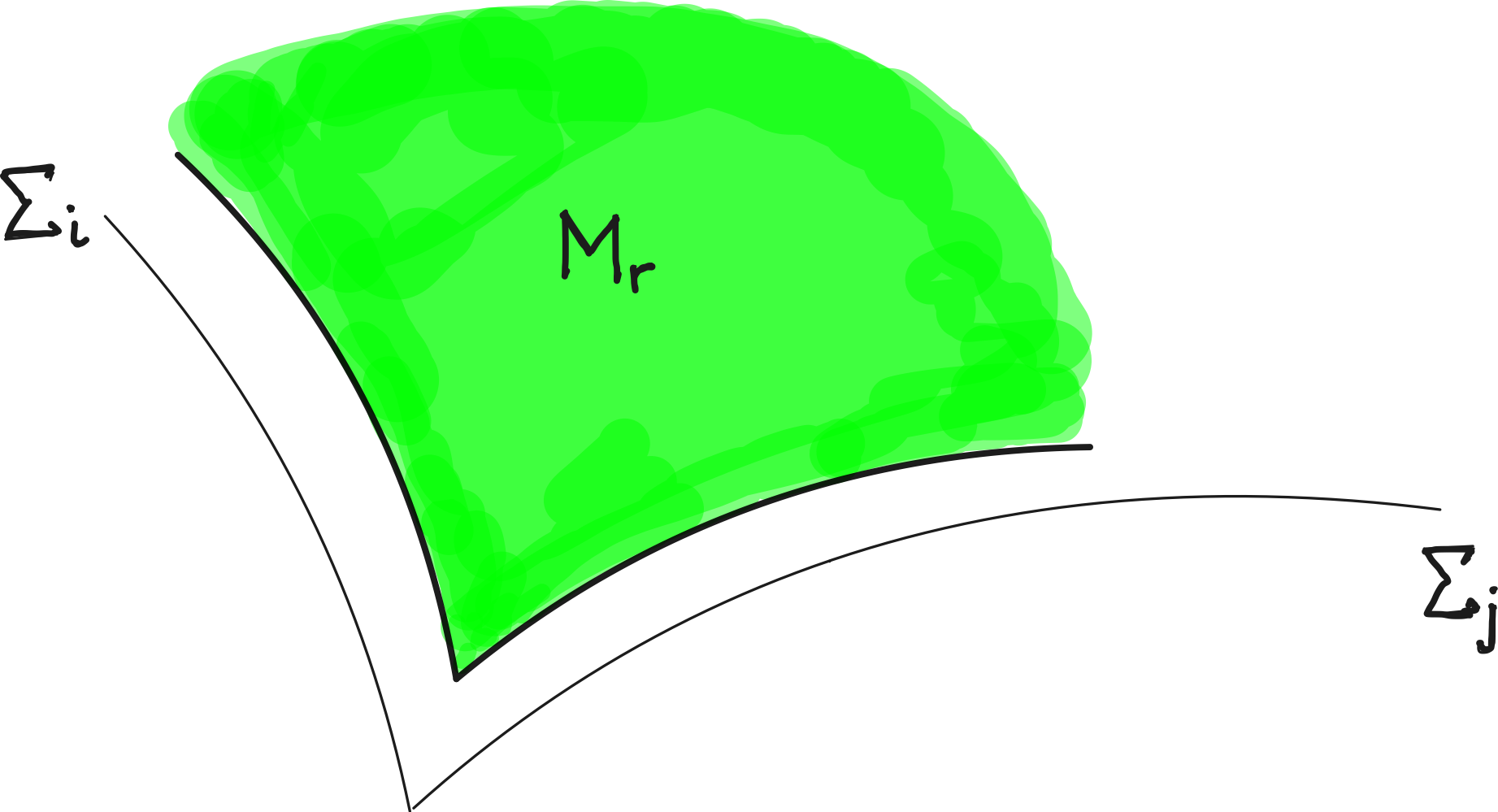
Let M 𝑀 M X ~ ~ 𝑋 \tilde{X} ρ : π 1 ( M ) → X ~ : 𝜌 → subscript 𝜋 1 𝑀 ~ 𝑋 \rho:\pi_{1}(M)\rightarrow\tilde{X} 1 dim ℂ M = n subscript dimension ℂ 𝑀 𝑛 \dim_{\mathbb{C}}M=n n 𝑛 n 5 M = M ¯ \ Σ 𝑀 \ ¯ 𝑀 Σ M=\bar{M}\backslash\Sigma M ¯ ¯ 𝑀 \bar{M} ≥ 2 absent 2 \geq 2 Σ Σ \Sigma
•
Y ¯ ⊂ M ¯ ¯ 𝑌 ¯ 𝑀 \bar{Y}\subset\bar{M} Y ¯ ∩ Σ ¯ 𝑌 Σ \bar{Y}\cap\Sigma
•
Y = Y ¯ \ Σ 𝑌 \ ¯ 𝑌 Σ Y=\bar{Y}\backslash\Sigma
•
ι : Y ↪ M : 𝜄 ↪ 𝑌 𝑀 \iota:Y\hookrightarrow M
•
ρ Y : π 1 ( Y ) → X ~ : subscript 𝜌 𝑌 → subscript 𝜋 1 𝑌 ~ 𝑋 \rho_{Y}:\pi_{1}(Y)\rightarrow\tilde{X} ρ Y = ρ ∘ ι ∗ subscript 𝜌 𝑌 𝜌 subscript 𝜄 \rho_{Y}=\rho\circ\iota_{*}
then there exists a unique pluriharmonic ρ Y subscript 𝜌 𝑌 \rho_{Y} u ~ Y : Y ~ → X ~ : subscript ~ 𝑢 𝑌 → ~ 𝑌 ~ 𝑋 \tilde{u}_{Y}:\tilde{Y}\rightarrow\tilde{X} { Y ¯ s } subscript ¯ 𝑌 𝑠 \{\bar{Y}_{s}\} M ¯ ¯ 𝑀 \bar{M} u ~ : M ~ → X ~ : ~ 𝑢 → ~ 𝑀 ~ 𝑋 \tilde{u}:\tilde{M}\rightarrow\tilde{X}
(0.1) u ~ = u ~ Y s on Y s := Y ¯ s \ Σ ~ 𝑢 subscript ~ 𝑢 subscript 𝑌 𝑠 on Y s := Y ¯ s \ Σ \tilde{u}=\tilde{u}_{Y_{s}}\mbox{ on $Y_{s}:=\bar{Y}_{s}\backslash\Sigma$}
is a well-defined, thereby proving the existence result for dim ℂ M = n subscript dimension ℂ 𝑀 𝑛 \dim_{\mathbb{C}}M=n n = 1 𝑛 1 n=1 n = 2 𝑛 2 n=2
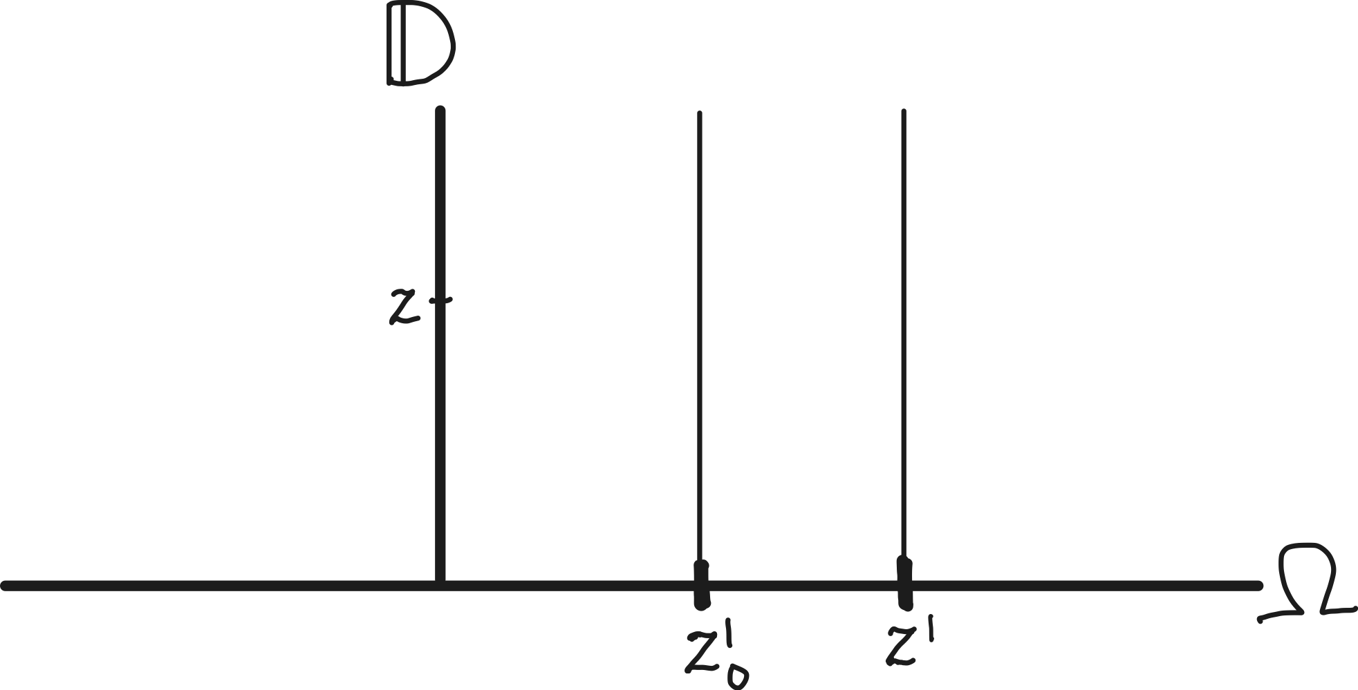
First assume dim ℂ M = 1 subscript dimension ℂ 𝑀 1 \dim_{\mathbb{C}}M=1 3 X ~ ~ 𝑋 \tilde{X} X 𝑋 X γ : 𝕊 1 → X : 𝛾 → superscript 𝕊 1 𝑋 \gamma:\mathbb{S}^{1}\rightarrow X X 𝑋 X γ 𝛾 \gamma E γ superscript 𝐸 𝛾 E^{\gamma} v 𝑣 v γ 𝛾 \gamma [ 0 , ∞ ) × 𝕊 1 0 superscript 𝕊 1 [0,\infty)\times\mathbb{S}^{1} γ 𝛾 \gamma { t } × 𝕊 1 𝑡 superscript 𝕊 1 \{t\}\times\mathbb{S}^{1} t 𝑡 t k : 𝕊 1 → X : 𝑘 → superscript 𝕊 1 𝑋 k:\mathbb{S}^{1}\rightarrow X
v : [ 1 , ∞ ) × 𝕊 1 → X : 𝑣 → 1 superscript 𝕊 1 𝑋 v:[1,\infty)\times\mathbb{S}^{1}\rightarrow X
be a Lipschitz continuous map with
v ( 1 , θ ) = k ( 1 , θ ) , 𝑣 1 𝜃 𝑘 1 𝜃 \displaystyle v(1,\theta)=k(1,\theta), ∀ θ ∈ 𝕊 1 , for-all 𝜃 superscript 𝕊 1 \displaystyle\forall\theta\in\mathbb{S}^{1},
v ( t , θ ) = γ ( θ ) , 𝑣 𝑡 𝜃 𝛾 𝜃 \displaystyle v(t,\theta)=\gamma(\theta), ∀ t ∈ [ 1 , ∞ ) , θ ∈ 𝕊 1 . formulae-sequence for-all 𝑡 1 𝜃 superscript 𝕊 1 \displaystyle\forall t\in[1,\infty),\,\theta\in\mathbb{S}^{1}.
The energy of v 𝑣 v [ 0 , T ] × 𝕊 1 0 𝑇 superscript 𝕊 1 [0,T]\times\mathbb{S}^{1} T ⋅ E γ + C ⋅ 𝑇 superscript 𝐸 𝛾 𝐶 T\cdot E^{\gamma}+C C 𝐶 C T 𝑇 T
u T : [ 0 , T ] × 𝕊 1 → X : subscript 𝑢 𝑇 → 0 𝑇 superscript 𝕊 1 𝑋 u_{T}:[0,T]\times\mathbb{S}^{1}\rightarrow X
be the Dirichlet solution on the finite cylinder [ 0 , T ] × 𝕊 1 0 𝑇 superscript 𝕊 1 [0,T]\times\mathbb{S}^{1} v 𝑣 v u T subscript 𝑢 𝑇 u_{T} u T subscript 𝑢 𝑇 u_{T} T ⋅ E γ + C ⋅ 𝑇 superscript 𝐸 𝛾 𝐶 T\cdot E^{\gamma}+C γ 𝛾 \gamma u T subscript 𝑢 𝑇 u_{T} [ 0 , t ] × 𝕊 1 0 𝑡 superscript 𝕊 1 [0,t]\times\mathbb{S}^{1} 0 < t ≤ T 0 𝑡 𝑇 0<t\leq T t ⋅ E γ ⋅ 𝑡 superscript 𝐸 𝛾 t\cdot E^{\gamma} u T subscript 𝑢 𝑇 u_{T} [ t 1 , t 2 ] × 𝕊 1 subscript 𝑡 1 subscript 𝑡 2 superscript 𝕊 1 [t_{1},t_{2}]\times\mathbb{S}^{1} T 𝑇 T ( t 2 − t 1 ) ⋅ E γ + C ⋅ subscript 𝑡 2 subscript 𝑡 1 superscript 𝐸 𝛾 𝐶 (t_{2}-t_{1})\cdot E^{\gamma}+C { u T } T ≥ 1 subscript subscript 𝑢 𝑇 𝑇 1 \{u_{T}\}_{T\geq 1} [ 0 , ∞ ) × 𝕊 1 0 superscript 𝕊 1 [0,\infty)\times\mathbb{S}^{1} T i → ∞ → subscript 𝑇 𝑖 T_{i}\rightarrow\infty u T i subscript 𝑢 subscript 𝑇 𝑖 u_{T_{i}} u : [ 0 , ∞ ) × 𝕊 1 → X : 𝑢 → 0 superscript 𝕊 1 𝑋 u:[0,\infty)\times\mathbb{S}^{1}\rightarrow X Σ Σ \Sigma γ 𝛾 \gamma ρ ( [ γ ] ) 𝜌 delimited-[] 𝛾 \rho([\gamma]) [ γ ] ∈ π 1 ( M ) delimited-[] 𝛾 subscript 𝜋 1 𝑀 [\gamma]\in\pi_{1}(M) [Loh ] . The main contribution of Chapter 3 6.5 6.6 n 𝑛 n 0.1
Next, assume dim ℂ M = 2 subscript dimension ℂ 𝑀 2 \dim_{\mathbb{C}}M=2 4 dim ℂ M = 1 subscript dimension ℂ 𝑀 1 \dim_{\mathbb{C}}M=1 [JZ , Sec. 3.2] ). By the assumption that the divisor Σ ⊂ M ¯ Σ ¯ 𝑀 \Sigma\subset\bar{M} Σ Σ \Sigma Σ j subscript Σ 𝑗 \Sigma_{j} σ j subscript 𝜎 𝑗 \sigma_{j} 𝒪 ( Σ j ) 𝒪 subscript Σ 𝑗 \mathcal{O}(\Sigma_{j}) Σ j subscript Σ 𝑗 \Sigma_{j} h j subscript ℎ 𝑗 h_{j} 𝒪 ( Σ j ) 𝒪 subscript Σ 𝑗 \mathcal{O}(\Sigma_{j}) M = M ¯ \ Σ 𝑀 \ ¯ 𝑀 Σ M=\bar{M}\backslash\Sigma g 𝑔 g 11.1 [CoGr ] ) making M 𝑀 M [M ] , we construct a fiber-wise harmonic map along the divisor at infinity. In other words, we construct a prototype map v 𝑣 v 𝔻 ∗ superscript 𝔻 \mathbb{D}^{*} 𝔻 𝔻 \mathbb{D} Σ j subscript Σ 𝑗 \Sigma_{j} v 𝑣 v 𝔻 ∗ superscript 𝔻 \mathbb{D}^{*} [ 0 , ∞ ) × 𝕊 1 0 superscript 𝕊 1 [0,\infty)\times\mathbb{S}^{1} v 𝑣 v M 𝑀 M ρ 𝜌 \rho u : M → X ~ : 𝑢 → 𝑀 ~ 𝑋 u:M\rightarrow\tilde{X} u 𝑢 u 9.8 2 [M , Section 6.3] in terms of flat vector bundles) allows us to prove pluriharmonicity and even holomorphicity of u 𝑢 u
In Chapter 6 [GS ] and to the Weil-Petersson completion of Teichmüller space developed in [DM1 ] , [DM2 ] , [DM3 ] and [DM4 ] with ideas in the previous chapters to prove Theorem 4 [RC , Proposition 2.1] (resp. Thurston’s classification of mapping classes and [DW ] ).
Chapter 1
§2 2
§3 3
Chapter 2
§4 4
§5 5
§6 2 6
Chapter 3
§7 7
§8 6.5 8
§9 6.6 9
Chapter 4
§10 10
§11 11
§12 12
§13 13
§14 14
§15 15
§16 4 16
Chapter 5
§17 17
§18 1 2 3 18
Chapter 6
§19 19
§20 4 5 20
Chapter 1 Preliminaries
1. Definitions
1.1. NPC spaces
We refer to [BH ] for more details than provided here.
Definition 1.1 .
A curve c : [ a , b ] → X ~ : 𝑐 → 𝑎 𝑏 ~ 𝑋 c:[a,b]\rightarrow\tilde{X} geodesic if 𝗅𝖾𝗇𝗀𝗍𝗁 ( l | [ α , β ] ) = d ( c ( α ) , c ( β ) ) 𝗅𝖾𝗇𝗀𝗍𝗁 evaluated-at 𝑙 𝛼 𝛽 𝑑 𝑐 𝛼 𝑐 𝛽 \mathsf{length}(l|_{[\alpha,\beta]})=d(c(\alpha),c(\beta)) [ α , β ] ⊂ [ a , b ] 𝛼 𝛽 𝑎 𝑏 [\alpha,\beta]\subset[a,b] X ~ ~ 𝑋 \tilde{X} geodesic space if there exists a geodesic connecting every pair of points in X ~ ~ 𝑋 \tilde{X}
Definition 1.2 .
An NPC space X ~ ~ 𝑋 \tilde{X} P , R , Q ∈ X ~ 𝑃 𝑅 𝑄
~ 𝑋 P,R,Q\in\tilde{X} c : [ 0 , l ] → X ~ : 𝑐 → 0 𝑙 ~ 𝑋 c:[0,l]\rightarrow\tilde{X} c ( 0 ) = Q 𝑐 0 𝑄 c(0)=Q c ( l ) = R 𝑐 𝑙 𝑅 c(l)=R
d 2 ( P , Q t ) ≤ ( 1 − t ) d 2 ( P , Q ) + t d 2 ( P , R ) − t ( 1 − t ) d 2 ( Q , R ) superscript 𝑑 2 𝑃 subscript 𝑄 𝑡 1 𝑡 superscript 𝑑 2 𝑃 𝑄 𝑡 superscript 𝑑 2 𝑃 𝑅 𝑡 1 𝑡 superscript 𝑑 2 𝑄 𝑅 d^{2}(P,Q_{t})\leq(1-t)d^{2}(P,Q)+td^{2}(P,R)-t(1-t)d^{2}(Q,R)
where Q t = c ( t l ) subscript 𝑄 𝑡 𝑐 𝑡 𝑙 Q_{t}=c(tl)
Notation 1.3 .
It follows immediately from Definition 1.2 P , Q ∈ X ~ 𝑃 𝑄
~ 𝑋 P,Q\in\tilde{X} t ∈ [ 0 , 1 ] 𝑡 0 1 t\in[0,1] unique point with distance from P 𝑃 P t d ( P , Q ) 𝑡 𝑑 𝑃 𝑄 td(P,Q) Q 𝑄 Q ( 1 − t ) d ( P , Q ) 1 𝑡 𝑑 𝑃 𝑄 (1-t)d(P,Q)
( 1 − t ) P + t Q . 1 𝑡 𝑃 𝑡 𝑄 (1-t)P+tQ.
Definition 1.4 .
Let X ~ ~ 𝑋 \tilde{X} c , c ′ : [ 0 , ∞ ) → X : 𝑐 superscript 𝑐 ′
→ 0 𝑋 c,c^{\prime}:[0,\infty)\rightarrow X equivalent if there exists a constant K 𝐾 K d ( c ( t ) , c ′ ( t ) ) ≤ K 𝑑 𝑐 𝑡 superscript 𝑐 ′ 𝑡 𝐾 d(c(t),c^{\prime}(t))\leq K t ∈ [ 0 , ∞ ) 𝑡 0 t\in[0,\infty) c 𝑐 c [ c ] delimited-[] 𝑐 [c] ∂ X ~ ~ 𝑋 \partial\tilde{X} X ~ ~ 𝑋 \tilde{X}
Definition 1.5 .
For any κ > 0 𝜅 0 \kappa>0 X ~ ~ 𝑋 \tilde{X} ( − κ ) 𝜅 (-\kappa) P , Q , R 𝑃 𝑄 𝑅
P,Q,R Q t subscript 𝑄 𝑡 Q_{t} 1.2
(1.1) cosh d ( P , Q t ) ≤ sinh ( 1 − t ) κ d ( P , Q ) sinh κ d ( P , Q ) ) cosh d ( P , Q ) + sinh t κ d ( P , Q ) sinh κ d ( P , Q ) ) cosh d ( P , R ) . \cosh d(P,Q_{t})\leq\frac{\sinh(1-t)\kappa d(P,Q)}{\sinh\kappa d(P,Q))}\cosh d(P,Q)+\frac{\sinh t\kappa d(P,Q)}{\sinh\kappa d(P,Q))}\cosh d(P,R).
Definition 1.6 .
We say that an NPC space X ~ ~ 𝑋 \tilde{X} negatively curved if, for any point P ∈ X ~ 𝑃 ~ 𝑋 P\in\tilde{X} r > 0 𝑟 0 r>0 κ > 0 𝜅 0 \kappa>0 P , Q , R ∈ B r ( P ) 𝑃 𝑄 𝑅
subscript 𝐵 𝑟 𝑃 P,Q,R\in B_{r}(P) 1.1
1.2. Maps into NPC spaces
In this paper, we consider harmonic maps into NPC spaces. In many cases, the target space X ~ ~ 𝑋 \tilde{X} u : Ω → X ~ : 𝑢 → Ω ~ 𝑋 u:\Omega\rightarrow\tilde{X}
E u = ∫ Ω | d f | 2 𝑑 vol g superscript 𝐸 𝑢 subscript Ω superscript 𝑑 𝑓 2 differential-d subscript vol 𝑔 E^{u}=\int_{\Omega}|df|^{2}d\mbox{vol}_{g}
where ( Ω , g ) Ω 𝑔 (\Omega,g) d vol g 𝑑 subscript vol 𝑔 d\mbox{vol}_{g} Ω Ω \Omega u : M ~ → X ~ : 𝑢 → ~ 𝑀 ~ 𝑋 u:\tilde{M}\rightarrow\tilde{X} harmonic if it is locally energy minimizing; i.e. for any p ∈ M ~ 𝑝 ~ 𝑀 p\in\tilde{M} r > 0 𝑟 0 r>0 u | B r ( p ) evaluated-at 𝑢 subscript 𝐵 𝑟 𝑝 u|_{B_{r}(p)} v : B r ( p ) → X ~ : 𝑣 → subscript 𝐵 𝑟 𝑝 ~ 𝑋 v:B_{r}(p)\rightarrow\tilde{X} u | B r ( p ) evaluated-at 𝑢 subscript 𝐵 𝑟 𝑝 u|_{B_{r}(p)}
In other cases, we consider the target X ~ ~ 𝑋 \tilde{X} [KS1 ] for more details than provided here.
Let ( Ω , g ) Ω 𝑔 (\Omega,g) Ω ϵ subscript Ω italic-ϵ \Omega_{\epsilon} Ω Ω \Omega ϵ italic-ϵ \epsilon ∂ Ω Ω \partial\Omega B ϵ ( x ) subscript 𝐵 italic-ϵ 𝑥 B_{\epsilon}(x) x 𝑥 x S ϵ ( x ) = ∂ B ϵ ( x ) subscript 𝑆 italic-ϵ 𝑥 subscript 𝐵 italic-ϵ 𝑥 S_{\epsilon}(x)=\partial B_{\epsilon}(x) f : Ω → X : 𝑓 → Ω 𝑋 f:\Omega\rightarrow X L 2 superscript 𝐿 2 L^{2} f ∈ L 2 ( Ω , X ) 𝑓 superscript 𝐿 2 Ω 𝑋 f\in L^{2}(\Omega,X)
∫ Ω d 2 ( f , P ) 𝑑 vol g < ∞ . subscript Ω superscript 𝑑 2 𝑓 𝑃 differential-d subscript vol 𝑔 \int_{\Omega}d^{2}(f,P)d\mbox{vol}_{g}<\infty.
For f ∈ L 2 ( Ω , X ) 𝑓 superscript 𝐿 2 Ω 𝑋 f\in L^{2}(\Omega,X)
e ϵ : Ω → 𝐑 , e ϵ ( x ) = { ∫ y ∈ S ϵ ( x ) d 2 ( f ( x ) , f ( y ) ) ϵ 2 d σ x , ϵ ϵ x ∈ Ω ϵ 0 otherwise : subscript 𝑒 italic-ϵ formulae-sequence → Ω 𝐑 subscript 𝑒 italic-ϵ 𝑥 cases subscript 𝑦 subscript 𝑆 italic-ϵ 𝑥 superscript 𝑑 2 𝑓 𝑥 𝑓 𝑦 superscript italic-ϵ 2 𝑑 subscript 𝜎 𝑥 italic-ϵ
italic-ϵ 𝑥 subscript Ω italic-ϵ 0 otherwise e_{\epsilon}:\Omega\rightarrow{\bf R},\ \ \ e_{\epsilon}(x)=\left\{\begin{array}[]{ll}\displaystyle{\int_{y\in S_{\epsilon}(x)}\frac{d^{2}(f(x),f(y))}{\epsilon^{2}}\frac{d\sigma_{x,\epsilon}}{\epsilon}}&x\in\Omega_{\epsilon}\\
0&\mbox{otherwise}\end{array}\right.
where σ x , ϵ subscript 𝜎 𝑥 italic-ϵ
\sigma_{x,\epsilon} S ϵ ( x ) subscript 𝑆 italic-ϵ 𝑥 S_{\epsilon}(x)
E ϵ f : C c ( X ) → 𝐑 , E ϵ f ( φ ) = ∫ Ω φ e ϵ 𝑑 vol g . : subscript superscript 𝐸 𝑓 italic-ϵ formulae-sequence → subscript 𝐶 𝑐 𝑋 𝐑 subscript superscript 𝐸 𝑓 italic-ϵ 𝜑 subscript Ω 𝜑 subscript 𝑒 italic-ϵ differential-d subscript vol 𝑔 E^{f}_{\epsilon}:C_{c}(X)\rightarrow{\bf R},\ \ \ \ E^{f}_{\epsilon}(\varphi)=\int_{\Omega}\varphi e_{\epsilon}d\mbox{vol}_{g}.
We say f 𝑓 f f ∈ W 1 , 2 ( Ω , X ) 𝑓 superscript 𝑊 1 2
Ω 𝑋 f\in W^{1,2}(\Omega,X)
E f := sup φ ∈ C c ( Ω ) , 0 ≤ φ ≤ 1 lim sup ϵ → 0 E ϵ f ( φ ) < ∞ . assign superscript 𝐸 𝑓 subscript supremum formulae-sequence 𝜑 subscript 𝐶 𝑐 Ω 0 𝜑 1 subscript limit-supremum → italic-ϵ 0 subscript superscript 𝐸 𝑓 italic-ϵ 𝜑 E^{f}:=\sup_{\varphi\in C_{c}(\Omega),0\leq\varphi\leq 1}\limsup_{\epsilon\rightarrow 0}E^{f}_{\epsilon}(\varphi)<\infty.
It is shown in [KS1 ] that if f 𝑓 f e ϵ ( x ) d vol g subscript 𝑒 italic-ϵ 𝑥 𝑑 subscript vol 𝑔 e_{\epsilon}(x)d\mbox{vol}_{g} e ( x ) 𝑒 𝑥 e(x) e ϵ ( x ) d vol g ⇀ e ( x ) d vol g ⇀ subscript 𝑒 italic-ϵ 𝑥 𝑑 subscript vol 𝑔 𝑒 𝑥 𝑑 subscript vol 𝑔 e_{\epsilon}(x)d\mbox{vol}_{g}\rightharpoonup e(x)d\mbox{vol}_{g} | ∇ f | 2 ( x ) superscript ∇ 𝑓 2 𝑥 |\nabla f|^{2}(x) e ( x ) 𝑒 𝑥 e(x) f 𝑓 f Ω Ω \Omega
E f [ Ω ] = ∫ Ω | ∇ f | 2 𝑑 vol g . superscript 𝐸 𝑓 delimited-[] Ω subscript Ω superscript ∇ 𝑓 2 differential-d subscript vol 𝑔 E^{f}[\Omega]=\int_{\Omega}|\nabla f|^{2}d\mbox{vol}_{g}.
Definition 1.7 .
We say a continuous map u : Ω → X ~ : 𝑢 → Ω ~ 𝑋 u:\Omega\rightarrow\tilde{X} Ω Ω \Omega harmonic if it is locally energy minimizing; more precisely, at each p ∈ Ω 𝑝 Ω p\in\Omega Ω Ω \Omega p 𝑝 p u 𝑢 u
For V ∈ Γ Ω 𝑉 Γ Ω V\in\Gamma\Omega Γ Ω Γ Ω \Gamma\Omega Ω Ω \Omega | f ∗ ( V ) | 2 superscript subscript 𝑓 𝑉 2 |f_{*}(V)|^{2} L 1 superscript 𝐿 1 L^{1} | f ∗ ( V ) | 2 superscript subscript 𝑓 𝑉 2 |f_{*}(V)|^{2} f 𝑓 f
π f ( V , W ) = Γ Ω × Γ Ω → L 1 ( Ω , 𝐑 ) subscript 𝜋 𝑓 𝑉 𝑊 Γ Ω Γ Ω → superscript 𝐿 1 Ω 𝐑 \pi_{f}(V,W)=\Gamma\Omega\times\Gamma\Omega\rightarrow L^{1}(\Omega,{\bf R})
where
π f ( V , W ) = 1 2 | f ∗ ( V + W ) | 2 − 1 2 | f ∗ ( V − W ) | 2 . subscript 𝜋 𝑓 𝑉 𝑊 1 2 superscript subscript 𝑓 𝑉 𝑊 2 1 2 superscript subscript 𝑓 𝑉 𝑊 2 \pi_{f}(V,W)=\frac{1}{2}|f_{*}(V+W)|^{2}-\frac{1}{2}|f_{*}(V-W)|^{2}.
We refer to [KS1 ] for more
details.
Let ( x 1 , … , x n ) superscript 𝑥 1 … superscript 𝑥 𝑛 (x^{1},\dots,x^{n}) ( Ω , g ) Ω 𝑔 (\Omega,g) g = ( g i j ) 𝑔 subscript 𝑔 𝑖 𝑗 g=(g_{ij}) g − 1 = ( g i j ) superscript 𝑔 1 superscript 𝑔 𝑖 𝑗 g^{-1}=(g^{ij}) f 𝑓 f [KS1 , (2.3vi)] )
| ∇ f | 2 = g i j π f ( ∂ ∂ x i , ∂ ∂ x j ) superscript ∇ 𝑓 2 superscript 𝑔 𝑖 𝑗 subscript 𝜋 𝑓 superscript 𝑥 𝑖 superscript 𝑥 𝑗 |\nabla f|^{2}=g^{ij}\pi_{f}(\frac{\partial}{\partial x^{i}},\frac{\partial}{\partial x^{j}})
Next assume ( Ω , g ) Ω 𝑔 (\Omega,g) ( z 1 = x 1 + i x 2 , … , z n = x 2 n − 1 + i x 2 n ) formulae-sequence superscript 𝑧 1 superscript 𝑥 1 𝑖 superscript 𝑥 2 …
superscript 𝑧 𝑛 superscript 𝑥 2 𝑛 1 𝑖 superscript 𝑥 2 𝑛 (z^{1}=x^{1}+ix^{2},\dots,z^{n}=x^{2n-1}+ix^{2n}) π f subscript 𝜋 𝑓 \pi_{f} ℂ ℂ \mathbb{C}
∂ f ∂ z i ⋅ ∂ f ∂ z ¯ j = π f ( ∂ ∂ z i , ∂ ∂ z ¯ j ) ⋅ 𝑓 superscript 𝑧 𝑖 𝑓 superscript ¯ 𝑧 𝑗 subscript 𝜋 𝑓 superscript 𝑧 𝑖 superscript ¯ 𝑧 𝑗 \frac{\partial f}{\partial z^{i}}\cdot\frac{\partial f}{\partial\bar{z}^{j}}=\pi_{f}(\frac{\partial}{\partial z^{i}},\frac{\partial}{\partial\bar{z}^{j}})
and
| ∂ f ∂ z i | 2 = π f ( ∂ ∂ z i , ∂ ∂ z ¯ i ) . superscript 𝑓 superscript 𝑧 𝑖 2 subscript 𝜋 𝑓 superscript 𝑧 𝑖 superscript ¯ 𝑧 𝑖 \left|\frac{\partial f}{\partial z^{i}}\right|^{2}=\pi_{f}(\frac{\partial}{\partial z^{i}},\frac{\partial}{\partial\bar{z}^{i}}).
Thus,
1 4 | ∇ f | 2 = g i j ¯ ∂ f ∂ z i ⋅ ∂ f ∂ z ¯ j . 1 4 superscript ∇ 𝑓 2 ⋅ superscript 𝑔 𝑖 ¯ 𝑗 𝑓 superscript 𝑧 𝑖 𝑓 superscript ¯ 𝑧 𝑗 \frac{1}{4}|\nabla f|^{2}=g^{i\bar{j}}\frac{\partial f}{\partial z^{i}}\cdot\frac{\partial f}{\partial\bar{z}^{j}}.
1.3. Isometries of an NPC space
Throughout this paper, we denote the group of isometries of an NPC space X ~ ~ 𝑋 \tilde{X} 𝖨𝗌𝗈𝗆 ( X ~ ) 𝖨𝗌𝗈𝗆 ~ 𝑋 \mathsf{Isom}(\tilde{X})
Definition 1.8 .
For I ∈ 𝖨𝗌𝗈𝗆 ( X ~ ) 𝐼 𝖨𝗌𝗈𝗆 ~ 𝑋 I\in\mathsf{Isom}(\tilde{X})
Δ I := inf P ∈ X ~ d ( I ( P ) , P ) assign subscript Δ 𝐼 subscript infimum 𝑃 ~ 𝑋 𝑑 𝐼 𝑃 𝑃 \Delta_{I}:=\inf_{P\in\tilde{X}}d(I(P),P)
denote its translation length and define
𝖬𝗂𝗇 ( I ) := { P ∈ X ~ : d ( I ( P ) , P ) = Δ I } . assign 𝖬𝗂𝗇 𝐼 conditional-set 𝑃 ~ 𝑋 𝑑 𝐼 𝑃 𝑃 subscript Δ 𝐼 \mathsf{Min}(I):=\{P\in\tilde{X}:d(I(P),P)=\Delta_{I}\}.
The isometry I 𝐼 I elliptic if Δ I = 0 subscript Δ 𝐼 0 \Delta_{I}=0 𝖬𝗂𝗇 ( I ) ≠ ∅ 𝖬𝗂𝗇 𝐼 \mathsf{Min}(I)\neq\emptyset hyperbolic if Δ I > 0 subscript Δ 𝐼 0 \Delta_{I}>0 𝖬𝗂𝗇 ( I ) ≠ ∅ 𝖬𝗂𝗇 𝐼 \mathsf{Min}(I)\neq\emptyset I 𝐼 I I 𝐼 I semisimple . Otherwise, I 𝐼 I parabolic .
Lemma 1.9 .
If X ~ ~ 𝑋 \tilde{X} I ∈ 𝖨𝗌𝗈𝗆 ( X ~ ) 𝐼 𝖨𝗌𝗈𝗆 ~ 𝑋 I\in\mathsf{Isom}(\tilde{X})
(1.2) c : [ 0 , ∞ ) → X ~ such that lim s → ∞ d ( I ( c ( s ) ) , c ( s ) ) = Δ I . : 𝑐 → 0 ~ 𝑋 such that subscript → 𝑠 𝑑 𝐼 𝑐 𝑠 𝑐 𝑠 subscript Δ 𝐼 c:[0,\infty)\rightarrow\tilde{X}\ \mbox{ such that }\ \lim_{s\rightarrow\infty}d(I(c(s)),c(s))=\Delta_{I}.
Proof.
Let P i ∈ X ~ subscript 𝑃 𝑖 ~ 𝑋 P_{i}\in\tilde{X}
lim i → ∞ d ( I ( P i ) , P i ) = Δ I . subscript → 𝑖 𝑑 𝐼 subscript 𝑃 𝑖 subscript 𝑃 𝑖 subscript Δ 𝐼 \lim_{i\rightarrow\infty}d(I(P_{i}),P_{i})=\Delta_{I}.
Fix P 0 ∈ X ~ subscript 𝑃 0 ~ 𝑋 P_{0}\in\tilde{X} T i = d ( P i , P 0 ) subscript 𝑇 𝑖 𝑑 subscript 𝑃 𝑖 subscript 𝑃 0 T_{i}=d(P_{i},P_{0}) 𝖬𝗂𝗇 ( I ) = ∅ 𝖬𝗂𝗇 𝐼 \mathsf{Min}(I)=\emptyset T i → ∞ → subscript 𝑇 𝑖 T_{i}\rightarrow\infty c i : [ 0 , T i ] → X ~ : subscript 𝑐 𝑖 → 0 subscript 𝑇 𝑖 ~ 𝑋 c_{i}:[0,T_{i}]\rightarrow\tilde{X} P 0 subscript 𝑃 0 P_{0} P i subscript 𝑃 𝑖 P_{i} X ~ ~ 𝑋 \tilde{X} c i ( s ) subscript 𝑐 𝑖 𝑠 c_{i}(s) c ( s ) 𝑐 𝑠 c(s)
Definition 1.10 .
Let Γ Γ \Gamma Λ Λ \Lambda Γ Γ \Gamma X ~ ~ 𝑋 \tilde{X} ρ : Γ → 𝖨𝗌𝗈𝗆 ( X ~ ) : 𝜌 → Γ 𝖨𝗌𝗈𝗆 ~ 𝑋 \rho:\Gamma\rightarrow\mathsf{Isom}(\tilde{X}) δ : X ~ → [ 0 , ∞ ) : 𝛿 → ~ 𝑋 0 \delta:\tilde{X}\rightarrow[0,\infty)
δ ( P ) = max { d ( ρ ( λ ) P , P ) : λ ∈ Λ } . 𝛿 𝑃 : 𝑑 𝜌 𝜆 𝑃 𝑃 𝜆 Λ \delta(P)=\max\{d(\rho(\lambda)P,P):\lambda\in\Lambda\}.
We say ρ 𝜌 \rho proper if the sublevel sets of the function δ 𝛿 \delta X ~ ~ 𝑋 \tilde{X} c > 0 𝑐 0 c>0 P 0 ∈ X subscript 𝑃 0 𝑋 P_{0}\in X R 0 > 0 subscript 𝑅 0 0 R_{0}>0
{ P ∈ X ~ : δ ( P ) ≤ c } ⊂ B R 0 ( P 0 ) . conditional-set 𝑃 ~ 𝑋 𝛿 𝑃 𝑐 subscript 𝐵 subscript 𝑅 0 subscript 𝑃 0 \{P\in\tilde{X}:\delta(P)\leq c\}\subset B_{R_{0}}(P_{0}).
1.4. Equivariant maps and section of the flat X ~ ~ 𝑋 \tilde{X}
Following Donaldson [Do ] , we will replace equivariant maps with sections of an associated fiber bundle.
Assume we have the following:
•
a complete Riemannian manifold ( M , g ) 𝑀 𝑔 (M,g) Π : M ~ → M : Π → ~ 𝑀 𝑀 \Pi:\tilde{M}\rightarrow M
•
•
action of π 1 ( M ) subscript 𝜋 1 𝑀 \pi_{1}(M) M ~ ~ 𝑀 \tilde{M}
•
homomorphism ρ : π 1 ( M ) → 𝖨𝗌𝗈𝗆 ( X ~ ) : 𝜌 → subscript 𝜋 1 𝑀 𝖨𝗌𝗈𝗆 ~ 𝑋 \rho:\pi_{1}(M)\rightarrow\mathsf{Isom}(\tilde{X})
Definition 1.11 .
A map f ~ : M ~ → X ~ : ~ 𝑓 → ~ 𝑀 ~ 𝑋 \tilde{f}:\tilde{M}\rightarrow\tilde{X} ρ 𝜌 \rho
f ~ ( γ p ) = ρ ( γ ) f ~ ( p ) , ∀ γ ∈ π 1 ( M ) , p ∈ M ~ . formulae-sequence ~ 𝑓 𝛾 𝑝 𝜌 𝛾 ~ 𝑓 𝑝 formulae-sequence for-all 𝛾 subscript 𝜋 1 𝑀 𝑝 ~ 𝑀 \tilde{f}(\gamma p)=\rho(\gamma)\tilde{f}(p),\ \ \forall\gamma\in\pi_{1}(M),\ p\in\tilde{M}.
The quotient space under the action of π 1 ( M ) subscript 𝜋 1 𝑀 \pi_{1}(M) M ~ × X ~ ~ 𝑀 ~ 𝑋 \tilde{M}\times\tilde{X} twisted product
M ~ × ρ X ~ . subscript 𝜌 ~ 𝑀 ~ 𝑋 \tilde{M}\times_{\rho}\tilde{X}.
In other words, M ~ × ρ X ~ subscript 𝜌 ~ 𝑀 ~ 𝑋 \tilde{M}\times_{\rho}\tilde{X} [ ( p , x ) ] delimited-[] 𝑝 𝑥 [(p,x)] ( p , x ) ∈ M ~ × X ~ 𝑝 𝑥 ~ 𝑀 ~ 𝑋 (p,x)\in\tilde{M}\times\tilde{X} γ ∈ π 1 ( M ) 𝛾 subscript 𝜋 1 𝑀 \gamma\in\pi_{1}(M) ρ ( γ ) 𝜌 𝛾 \rho(\gamma)
M ~ × ρ X ~ → M → subscript 𝜌 ~ 𝑀 ~ 𝑋 𝑀 \tilde{M}\times_{\rho}\tilde{X}\rightarrow M
with fibers over p ∈ M 𝑝 𝑀 p\in M X ~ ~ 𝑋 \tilde{X} flat X ~ ~ 𝑋 \tilde{X} over M 𝑀 M ρ 𝜌 \rho
There is a one-to-one correspondence between sections of this fibration and ρ 𝜌 \rho
f ~ : M ~ → X ~ ⟷ f : M → M ~ × ρ X ~ : ~ 𝑓 → ~ 𝑀 ~ 𝑋 ⟷ 𝑓
: → 𝑀 subscript 𝜌 ~ 𝑀 ~ 𝑋 \tilde{f}:\tilde{M}\rightarrow\tilde{X}\ \ \ \ \longleftrightarrow\ \ \ \ f:M\rightarrow\tilde{M}\times_{\rho}\tilde{X}
satisfying the relationship
[ ( p ~ , f ~ ( p ~ ) ) ] ↔ f ( p ) where Π ( p ~ ) = p . ↔ delimited-[] ~ 𝑝 ~ 𝑓 ~ 𝑝 𝑓 𝑝 where Π ( p ~ ) = p . [(\tilde{p},\tilde{f}(\tilde{p}))]\leftrightarrow f(p)\ \mbox{
where $\Pi(\tilde{p})=p$.}
Since the energy density function | ∇ f ~ | 2 superscript ∇ ~ 𝑓 2 |\nabla\tilde{f}|^{2} f ~ ~ 𝑓 \tilde{f} ρ 𝜌 \rho
| ∇ f | 2 ( p ) := | ∇ f ~ | 2 ( p ~ ) . assign superscript ∇ 𝑓 2 𝑝 superscript ∇ ~ 𝑓 2 ~ 𝑝 |\nabla f|^{2}(p):=|\nabla\tilde{f}|^{2}(\tilde{p}).
(In literature, this quantity is sometimes referred as the vertical part the derivative of f 𝑓 f [Do ] .)
We can similarly define the pullback inner product and directional energy density functions of f 𝑓 f f ~ ~ 𝑓 \tilde{f} 1.2 U ⊂ M 𝑈 𝑀 U\subset M f 𝑓 f
(1.3) E f [ U ] = ∫ U | ∇ f | 2 𝑑 vol g . superscript 𝐸 𝑓 delimited-[] 𝑈 subscript 𝑈 superscript ∇ 𝑓 2 differential-d subscript vol 𝑔 E^{f}[U]=\int_{U}|\nabla f|^{2}d\mbox{vol}_{g}.
Furthermore,
for sections f 1 subscript 𝑓 1 f_{1} f 2 subscript 𝑓 2 f_{2}
(1.4) d ( f 1 ( p ) , f 2 ( p ) ) := d ( f ~ 1 ( p ~ ) , f ~ 2 ( p ~ ) ) assign 𝑑 subscript 𝑓 1 𝑝 subscript 𝑓 2 𝑝 𝑑 subscript ~ 𝑓 1 ~ 𝑝 subscript ~ 𝑓 2 ~ 𝑝 d(f_{1}(p),f_{2}(p)):=d(\tilde{f}_{1}(\tilde{p}),\tilde{f}_{2}(\tilde{p}))
where f ~ 1 subscript ~ 𝑓 1 \tilde{f}_{1} f ~ 2 subscript ~ 𝑓 2 \tilde{f}_{2} ρ 𝜌 \rho f 1 subscript 𝑓 1 f_{1} f 2 subscript 𝑓 2 f_{2}
2. Exponential decay of an isometry
The distinguishing characteristic of a semisimple isometry I : X ~ → X ~ : 𝐼 → ~ 𝑋 ~ 𝑋 I:\tilde{X}\rightarrow\tilde{X} P ∗ ∈ X ~ subscript 𝑃 ~ 𝑋 P_{*}\in\tilde{X} d ( P ∗ , I ( P ∗ ) ) 𝑑 subscript 𝑃 𝐼 subscript 𝑃 d(P_{*},I(P_{*})) Δ I subscript Δ 𝐼 \Delta_{I} P ∗ subscript 𝑃 P_{*} I 𝐼 I
Definition 2.1 .
We say that I ∈ 𝖨𝗌𝗈𝗆 ( X ~ ) 𝐼 𝖨𝗌𝗈𝗆 ~ 𝑋 I\in\mathsf{Isom}(\tilde{X}) exponential decay to its translation length (or simply exponential decay for short) if one of the following conditions hold:
•
•
I 𝐼 I c : [ 0 , ∞ ) → X ~ : 𝑐 → 0 ~ 𝑋 c:[0,\infty)\rightarrow\tilde{X} a , b > 0 𝑎 𝑏
0 a,b>0
d 2 ( I ( c ( t ) ) , c ( t ) ) ≤ Δ I 2 ( 1 + b e − a t ) . superscript 𝑑 2 𝐼 𝑐 𝑡 𝑐 𝑡 superscript subscript Δ 𝐼 2 1 𝑏 superscript 𝑒 𝑎 𝑡 d^{2}(I(c(t)),c(t))\leq\Delta_{I}^{2}(1+be^{-at}).
If I 𝐼 I c ( t ) 𝑐 𝑡 c(t) P ∗ subscript 𝑃 P_{*} I 𝐼 I c ( t ) 𝑐 𝑡 c(t) d ( c ( t ) , I ( c ( t ) ) ) 𝑑 𝑐 𝑡 𝐼 𝑐 𝑡 d(c(t),I(c(t))) Δ I subscript Δ 𝐼 \Delta_{I}
In this section, we prove that isometries of important examples of NPC spaces (i.e. symmetric spaces of non-compact type, CAT(− 1 1 -1
2.1. Symmetric spaces of non-compact type
In this subsection, we prove that every isometry of a symmetric space of non-compact type has exponential decay. To this end, we introduce the following notations:
•
𝖬 ( n , ℝ ) 𝖬 𝑛 ℝ \mathsf{M}(n,\mathbb{R}) ( n × n ) 𝑛 𝑛 (n\times n)
•
𝖲 ( n , ℝ ) 𝖲 𝑛 ℝ \mathsf{S}(n,\mathbb{R}) 𝖬 ( n , ℝ ) 𝖬 𝑛 ℝ \mathsf{M}(n,\mathbb{R})
•
𝖯 ( n , ℝ ) 𝖯 𝑛 ℝ \mathsf{P}(n,\mathbb{R})
•
𝖦𝖫 ( n , ℝ ) 𝖦𝖫 𝑛 ℝ \mathsf{GL}(n,\mathbb{R}) ( n × n ) 𝑛 𝑛 (n\times n)
•
𝖮 ( n ) 𝖮 𝑛 \mathsf{O}(n) 𝖦𝖫 ( n , ℝ ) 𝖦𝖫 𝑛 ℝ \mathsf{GL}(n,\mathbb{R})
•
𝖠 ( n ) 𝖠 𝑛 \mathsf{A}(n)
•
𝖭 ( n ) 𝖭 𝑛 \mathsf{N}(n)
The group 𝖦𝖫 ( n , ℝ ) 𝖦𝖫 𝑛 ℝ \mathsf{GL}(n,\mathbb{R}) 𝖯 ( n , ℝ ) 𝖯 𝑛 ℝ \mathsf{P}(n,\mathbb{R})
G . p := G p G T , ∀ G ∈ 𝖦𝖫 ( n , ℝ ) , p ∈ 𝖯 ( n , ℝ ) formulae-sequence 𝐺 formulae-sequence assign 𝑝 𝐺 𝑝 superscript 𝐺 𝑇 formulae-sequence for-all 𝐺 𝖦𝖫 𝑛 ℝ 𝑝 𝖯 𝑛 ℝ G.p:=GpG^{T},\ \ \ \forall G\in\mathsf{GL}(n,\mathbb{R}),\,p\in\mathsf{P}(n,\mathbb{R})
where the left hand side consists of matrix multiplication.
Denoting the identity matrix by e 𝑒 e
T e 𝖯 ( n , ℝ ) = 𝖲 ( n , ℝ ) . subscript 𝑇 𝑒 𝖯 𝑛 ℝ 𝖲 𝑛 ℝ T_{e}\mathsf{P}(n,\mathbb{R})=\mathsf{S}(n,\mathbb{R}).
The manifold 𝖯 ( n , ℝ ) 𝖯 𝑛 ℝ \mathsf{P}(n,\mathbb{R})
⟨ V , W ⟩ p = Trace ( p − 1 V p − 1 W ) , p ∈ 𝖯 ( n , ℝ ) , V , W ∈ T p 𝖯 ( n , ℝ ) formulae-sequence subscript 𝑉 𝑊
𝑝 Trace superscript 𝑝 1 𝑉 superscript 𝑝 1 𝑊 formulae-sequence 𝑝 𝖯 𝑛 ℝ 𝑉
𝑊 subscript 𝑇 𝑝 𝖯 𝑛 ℝ \langle V,W\rangle_{p}=\mbox{Trace}(p^{-1}Vp^{-1}W),\ \ \ p\in\mathsf{P}(n,\mathbb{R}),\ V,W\in T_{p}\mathsf{P}(n,\mathbb{R})
defines a NPC symmetric space with isometry group 𝖨𝗌𝗈𝗆 ( 𝖯 ( n , ℝ ) ) = 𝖦𝖫 ( n , ℝ ) 𝖨𝗌𝗈𝗆 𝖯 𝑛 ℝ 𝖦𝖫 𝑛 ℝ \mathsf{Isom}(\mathsf{P}(n,\mathbb{R}))=\mathsf{GL}(n,\mathbb{R}) [BH , II.10.33, II.10.34, II.10.39] ).
Let e 𝑒 e 𝖯 ( n , ℝ ) 𝖯 𝑛 ℝ \mathsf{P}(n,\mathbb{R})
c : ℝ → 𝖯 ( n , ℝ ) with c ( 0 ) = e and c ′ ( 0 ) = V ∈ T e 𝖯 ( n , ℝ ) = 𝖲 ( n , ℝ ) : 𝑐 → ℝ 𝖯 𝑛 ℝ with c ( 0 ) = e and c ′ ( 0 ) = V ∈ T e 𝖯 ( n , ℝ ) = 𝖲 ( n , ℝ ) c:\mathbb{R}\rightarrow\mathsf{P}(n,\mathbb{R})\mbox{ \ with $c(0)=e$ and $c^{\prime}(0)=V\in T_{e}\mathsf{P}(n,\mathbb{R})=\mathsf{S}(n,\mathbb{R})$}
is given by c ( t ) = exp ( t V ) 𝑐 𝑡 𝑡 𝑉 c(t)=\exp(tV) p = exp ( V ) 𝑝 𝑉 p=\exp(V) d ( e , p ) = | V | 𝑑 𝑒 𝑝 𝑉 d(e,p)=|V| [BH , II.10.42] ).
Definition 2.2 .
For a geodesic ray c : [ 0 , ∞ ) → 𝖯 ( n , ℝ ) : 𝑐 → 0 𝖯 𝑛 ℝ c:[0,\infty)\rightarrow\mathsf{P}(n,\mathbb{R}) ξ = [ c ] ∈ ∂ 𝖯 ( n , ℝ ) 𝜉 delimited-[] 𝑐 𝖯 𝑛 ℝ \xi=[c]\in\partial\mathsf{P}(n,\mathbb{R}) c 𝑐 c parabolic subgroup associated to ξ = [ c ] 𝜉 delimited-[] 𝑐 \xi=[c]
𝖦 ξ := { G ∈ 𝖯 ( n , ℝ ) : G . ξ = ξ } . assign subscript 𝖦 𝜉 conditional-set 𝐺 𝖯 𝑛 ℝ formulae-sequence 𝐺 𝜉 𝜉 {\mathsf{G}}_{\xi}:=\{G\in\mathsf{P}(n,\mathbb{R}):G.\xi=\xi\}.
The horospherical subgroup associated to ξ = [ c ] 𝜉 delimited-[] 𝑐 \xi=[c]
𝖭 ξ = { G ∈ G ξ : exp ( − t V ) G exp ( t V ) → I as t → ∞ } . subscript 𝖭 𝜉 conditional-set 𝐺 subscript 𝐺 𝜉 → 𝑡 𝑉 𝐺 𝑡 𝑉 𝐼 as 𝑡 → {\mathsf{N}}_{\xi}=\{G\in G_{\xi}:\exp(-tV)G\exp(tV)\rightarrow I\mbox{ as }t\rightarrow\infty\}.
We refer to [BH , 10.62] for details regarding these subgroups.
Following an argument of [M ] , we will first prove that all isometries of 𝖯 ( n , ℝ ) 𝖯 𝑛 ℝ \mathsf{P}(n,\mathbb{R})
Definition 2.3 .
For G ∈ 𝖦𝖫 ( n , ℝ ) 𝐺 𝖦𝖫 𝑛 ℝ G\in\mathsf{GL}(n,\mathbb{R})
ρ ( G ) := ( ∑ i = 1 n ( log | b i | 2 ) 2 ) 1 2 assign 𝜌 𝐺 superscript superscript subscript 𝑖 1 𝑛 superscript superscript subscript 𝑏 𝑖 2 2 1 2 \rho(G):=\left(\sum_{i=1}^{n}(\log|b_{i}|^{2})^{2}\right)^{\frac{1}{2}}
where b 1 , … , b n subscript 𝑏 1 … subscript 𝑏 𝑛
b_{1},\dots,b_{n} G 𝐺 G
Lemma 2.4 .
The translation length of G ∈ 𝖦𝖫 ( n , ℝ ) 𝐺 𝖦𝖫 𝑛 ℝ G\in\mathsf{GL}(n,\mathbb{R}) ρ ( G ) 𝜌 𝐺 \rho(G) ρ ( G ) ≤ Δ G . 𝜌 𝐺 subscript Δ 𝐺 \rho(G)\leq\Delta_{G}.
Proof.
We need to show
(2.1) ρ ( G ) ≤ d ( p , G . p ) , ∀ p ∈ 𝖯 ( n , ℝ ) , ∀ G ∈ 𝖦𝖫 ( n , ℝ ) . \rho(G)\leq d(p,G.p),\ \ \forall p\in\mathsf{P}(n,\mathbb{R}),\forall G\in\mathsf{GL}(n,\mathbb{R}).
Before we proceed, note the following:
•
It is sufficient to prove the inequality of (2.1 p 𝑝 p e 𝑒 e 𝖯 ( n , ℝ ) 𝖯 𝑛 ℝ \mathsf{P}(n,\mathbb{R})
We prove this claim in two steps.
–
Let q 𝑞 q q = 𝖽𝗂𝖺𝗀 ( λ 1 , … , λ n ) 𝑞 𝖽𝗂𝖺𝗀 subscript 𝜆 1 … subscript 𝜆 𝑛 q=\mathsf{diag}(\lambda_{1},\dots,\lambda_{n}) q 1 2 = 𝖽𝗂𝖺𝗀 ( λ 1 1 2 , … , λ n 1 2 ) superscript 𝑞 1 2 𝖽𝗂𝖺𝗀 superscript subscript 𝜆 1 1 2 … superscript subscript 𝜆 𝑛 1 2 q^{\frac{1}{2}}=\mathsf{diag}(\lambda_{1}^{\frac{1}{2}},\dots,\lambda_{n}^{\frac{1}{2}}) q = q 1 2 e q 1 2 𝑞 superscript 𝑞 1 2 𝑒 superscript 𝑞 1 2 q=q^{\frac{1}{2}}eq^{\frac{1}{2}} G 0 ∈ 𝖦𝖫 ( n , ℝ ) subscript 𝐺 0 𝖦𝖫 𝑛 ℝ G_{0}\in\mathsf{GL}(n,\mathbb{R}) G 1 := q − 1 2 G 0 q 1 2 assign subscript 𝐺 1 superscript 𝑞 1 2 subscript 𝐺 0 superscript 𝑞 1 2 G_{1}:=q^{-\frac{1}{2}}G_{0}q^{\frac{1}{2}}
d ( G 0 . q , q ) \displaystyle d(G_{0}.q,q) = \displaystyle= d ( G 0 q G 0 t , q ) = d ( G 0 q 1 2 e q 1 2 G 0 t , q 1 2 e q 1 2 ) 𝑑 subscript 𝐺 0 𝑞 superscript subscript 𝐺 0 𝑡 𝑞 𝑑 subscript 𝐺 0 superscript 𝑞 1 2 𝑒 superscript 𝑞 1 2 superscript subscript 𝐺 0 𝑡 superscript 𝑞 1 2 𝑒 superscript 𝑞 1 2 \displaystyle d(G_{0}qG_{0}^{t},q)\ =\ d(G_{0}q^{\frac{1}{2}}eq^{\frac{1}{2}}G_{0}^{t},\,q^{\frac{1}{2}}eq^{\frac{1}{2}})
= \displaystyle= d ( q − 1 2 G 0 q 1 2 e q 1 2 G 0 t q − 1 2 , e ) = d ( G 1 . e , e ) . \displaystyle d(q^{-\frac{1}{2}}G_{0}q^{\frac{1}{2}}eq^{\frac{1}{2}}G_{0}^{t}q^{-\frac{1}{2}},e)\ =\ d(G_{1}.e,e).
–
Let p ∈ 𝖯 ( n , ℝ ) 𝑝 𝖯 𝑛 ℝ p\in\mathsf{P}(n,\mathbb{R}) O ∈ 𝖮 ( n ) 𝑂 𝖮 𝑛 O\in\mathsf{O}(n) p = O q O t = O . q formulae-sequence 𝑝 𝑂 𝑞 superscript 𝑂 𝑡 𝑂 𝑞 p=OqO^{t}=O.q q 𝑞 q G 0 := O G O t assign subscript 𝐺 0 𝑂 𝐺 superscript 𝑂 𝑡 G_{0}:=OGO^{t} G 1 := q − 1 2 G 0 q 1 2 assign subscript 𝐺 1 superscript 𝑞 1 2 subscript 𝐺 0 superscript 𝑞 1 2 G_{1}:=q^{-\frac{1}{2}}G_{0}q^{\frac{1}{2}}
d ( G . p , p ) \displaystyle d(G.p,p) = \displaystyle= d ( G O . q , O . q ) = d ( O t G O . q , q ) \displaystyle d(GO.q,\,O.q)\ =\ d(O^{t}GO.q,q)
= \displaystyle= d ( G 0 . q , q ) = d ( G 1 . e , e ) \displaystyle d(G_{0}.q,q)\ =\ d(G_{1}.e,e)
and ρ ( G ) = ρ ( G 1 ) 𝜌 𝐺 𝜌 subscript 𝐺 1 \rho(G)=\rho(G_{1})
•
It is sufficient to prove (2.1 G 𝐺 G Indeed, if G 𝐺 G G ( j ) superscript 𝐺 𝑗 G^{(j)} ρ ( G ( j ) ) → ρ ( G ) → 𝜌 superscript 𝐺 𝑗 𝜌 𝐺 \rho(G^{(j)})\rightarrow\rho(G) d ( G ( j ) . e , e ) → d ( G . e , e ) d(G^{(j)}.e,e)\rightarrow d(G.e,e)
By virtue of the above two bullet points, we assume that G ∈ 𝖦𝖫 ( n , ℝ ) 𝐺 𝖦𝖫 𝑛 ℝ G\in\mathsf{GL}(n,\mathbb{R}) b 1 , b 2 , … , b n subscript 𝑏 1 subscript 𝑏 2 … subscript 𝑏 𝑛
b_{1},b_{2},\dots,b_{n} 2.1 p = e 𝑝 𝑒 p=e
Let V ∈ T e 𝖯 ( n , ℝ ) = 𝖲 ( n , ℝ ) 𝑉 subscript 𝑇 𝑒 𝖯 𝑛 ℝ 𝖲 𝑛 ℝ V\in T_{e}\mathsf{P}(n,\mathbb{R})=\mathsf{S}(n,\mathbb{R})
log | b 1 | 2 ρ ( G ) , log | b 2 | 2 ρ ( G ) , … , log | b n | 2 ρ ( G ) . superscript subscript 𝑏 1 2 𝜌 𝐺 superscript subscript 𝑏 2 2 𝜌 𝐺 … superscript subscript 𝑏 𝑛 2 𝜌 𝐺
\frac{\log|b_{1}|^{2}}{\rho(G)},\ \frac{\log|b_{2}|^{2}}{\rho(G)},\ \dots,\frac{\log|b_{n}|^{2}}{\rho(G)}.
Conjugating by elemen
Let c ( t ) = exp ( t V ) 𝑐 𝑡 𝑡 𝑉 c(t)=\exp(tV) ξ = [ c ] 𝜉 delimited-[] 𝑐 \xi=[c] G = O A 0 N 𝐺 𝑂 subscript 𝐴 0 𝑁 G=OA_{0}N O ∈ 𝖮 ( n ) 𝑂 𝖮 𝑛 O\in\mathsf{O}(n) A 0 ∈ 𝖠 ( n ) subscript 𝐴 0 𝖠 𝑛 A_{0}\in\mathsf{A}(n) N ∈ 𝖭 ( n ) 𝑁 𝖭 𝑛 N\in\mathsf{N}(n) A ′ = A 0 N superscript 𝐴 ′ subscript 𝐴 0 𝑁 A^{\prime}=A_{0}N A ′ = N ′ A 0 superscript 𝐴 ′ superscript 𝑁 ′ subscript 𝐴 0 A^{\prime}=N^{\prime}A_{0} N ′ ∈ 𝖭 ( n ) superscript 𝑁 ′ 𝖭 𝑛 N^{\prime}\in\mathsf{N}(n)
G = O A 0 N = O A ′ = O N ′ A 0 . 𝐺 𝑂 subscript 𝐴 0 𝑁 𝑂 superscript 𝐴 ′ 𝑂 superscript 𝑁 ′ subscript 𝐴 0 G=OA_{0}N=OA^{\prime}=ON^{\prime}A_{0}.
The diagonal matrix A 0 subscript 𝐴 0 A_{0} c ( t ) = exp ( t V ) 𝑐 𝑡 𝑡 𝑉 c(t)=\exp(tV) N 𝑁 N 𝖭 ξ subscript 𝖭 𝜉 {\mathsf{N}}_{\xi} ξ 𝜉 \xi [BH , II.10.66] ).
By construction,
c ( ρ ( G ) ) = exp ( ρ ( G ) V ) = A 0 A 0 T = A 0 . e . formulae-sequence 𝑐 𝜌 𝐺 𝜌 𝐺 𝑉 subscript 𝐴 0 superscript subscript 𝐴 0 𝑇 subscript 𝐴 0 𝑒 c(\rho(G))=\exp(\rho(G)V)=A_{0}A_{0}^{T}=A_{0}.e.
Since the geodesic line c ( t ) 𝑐 𝑡 c(t) ξ = [ c ] 𝜉 delimited-[] 𝑐 \xi=[c] A 0 . e formulae-sequence subscript 𝐴 0 𝑒 A_{0}.e e 𝑒 e A 0 . e formulae-sequence subscript 𝐴 0 𝑒 A_{0}.e [BH , I.10.5] ). Furthermore, any orbit of N ′ superscript 𝑁 ′ N^{\prime} [BH , II.10.66] ), and hence
d ( A 0 . e , e ) ≤ d ( N ′ A 0 . e , e ) = d ( G . e , e ) . d(A_{0}.e,e)\leq d(N^{\prime}A_{0}.e,\,e)=d(G.e,e).
This in turn implies
ρ ( G ) = ρ ( A 0 ) = d ( A 0 . e , e ) ≤ d ( G . e , e ) . \rho(G)=\rho(A_{0})=d(A_{0}.e,e)\leq d(G.e,e).
∎
Theorem 2.5 .
For a parabolic element G ∈ 𝖯 ( n , ℝ ) 𝐺 𝖯 𝑛 ℝ G\in\mathsf{P}(n,\mathbb{R})
•
ξ ∈ ∂ 𝖯 ( n , ℝ ) 𝜉 𝖯 𝑛 ℝ \xi\in\partial\mathsf{P}(n,\mathbb{R}) be such that G ∈ 𝖦 ξ 𝐺 subscript 𝖦 𝜉 G\in{\mathsf{G}}_{\xi} (i.e. G 𝐺 G is an element of the parabolic subgroup associated to ξ 𝜉 \xi ),
•
c : [ 0 , ∞ ) → 𝖯 ( n , ℝ ) : 𝑐 → 0 𝖯 𝑛 ℝ c:[0,\infty)\rightarrow\mathsf{P}(n,\mathbb{R}) be the geodesic ray such that ξ = [ c ] 𝜉 delimited-[] 𝑐 \xi=[c] and c ( 0 ) = e 𝑐 0 𝑒 c(0)=e (cf. [ BH , 10.62] ).
Then there exist constants a , b > 0 𝑎 𝑏
0 a,b>0
lim t → ∞ d ( c ( t ) , G . c ( t ) ) = △ G + b e − a t . \lim_{t\rightarrow\infty}d(c(t),G.c(t))=\triangle_{G}+be^{-at}.
Proof.
We will prove this by an inductive argument on n 𝑛 n
V ∈ T e ( 𝖯 ( n , ℝ ) ) = 𝖲 ( n , ℝ ) such that c ( t ) = exp ( t V ) . 𝑉 subscript 𝑇 𝑒 𝖯 𝑛 ℝ 𝖲 𝑛 ℝ such that 𝑐 𝑡 𝑡 𝑉 V\in T_{e}(\mathsf{P}(n,\mathbb{R}))=\mathsf{S}(n,\mathbb{R})\mbox{ such that }c(t)=\exp(tV).
By conjugating by an element of 𝖲𝖮 ( n ) 𝖲𝖮 𝑛 \mathsf{SO}(n) V 𝑉 V
V = 𝖽𝗂𝖺𝗀 ( λ 1 , … , λ n ) with λ 1 ≥ ⋯ ≥ λ n . 𝑉 𝖽𝗂𝖺𝗀 subscript 𝜆 1 … subscript 𝜆 𝑛 with λ 1 ≥ ⋯ ≥ λ n V=\mathsf{diag}(\lambda_{1},\dots,\lambda_{n})\mbox{
with $\lambda_{1}\geq\dots\geq\lambda_{n}$}.
Let r 1 , … , r k subscript 𝑟 1 … subscript 𝑟 𝑘
r_{1},\dots,r_{k} [BH , 10.64] ,
where
•
A 𝐴 A
(2.2) A = ( A 11 0 … 0 0 A 22 … 0 … … … … 0 0 … A k k ) 𝐴 matrix subscript 𝐴 11 0 … 0 0 subscript 𝐴 22 … 0 … … … … 0 0 … subscript 𝐴 𝑘 𝑘 A=\begin{pmatrix}A_{11}&0&\dots&0\\
0&A_{22}&\dots&0\\
\dots&\dots&\dots&\dots\\
0&0&\dots&A_{kk}\end{pmatrix}
•
N ∈ 𝖭 ξ 𝑁 subscript 𝖭 𝜉 N\in{\mathsf{N}}_{\xi} ξ ∈ [ c 0 ] 𝜉 delimited-[] subscript 𝑐 0 \xi\in[c_{0}] N 𝑁 N
(2.3) N = ( I r 1 A 12 … A 1 k 0 I r 2 … A 2 k … … … … 0 0 … I r k ) 𝑁 matrix subscript 𝐼 subscript 𝑟 1 subscript 𝐴 12 … subscript 𝐴 1 𝑘 0 subscript 𝐼 subscript 𝑟 2 … subscript 𝐴 2 𝑘 … … … … 0 0 … subscript 𝐼 subscript 𝑟 𝑘 N=\begin{pmatrix}I_{r_{1}}&A_{12}&\dots&A_{1k}\\
0&I_{r_{2}}&\dots&A_{2k}\\
\dots&\dots&\dots&\dots\\
0&0&\dots&I_{r_{k}}\end{pmatrix}
where A i j subscript 𝐴 𝑖 𝑗 A_{ij} ( r j × r j ) subscript 𝑟 𝑗 subscript 𝑟 𝑗 (r_{j}\times r_{j}) I i j subscript 𝐼 𝑖 𝑗 I_{ij} ( r j × r j ) subscript 𝑟 𝑗 subscript 𝑟 𝑗 (r_{j}\times r_{j})
Let F ( c ) 𝐹 𝑐 F(c) c 𝑐 c [BH , 10.67] )
(2.4) F ( c ) = ( 𝖯 ( r 1 , ℝ ) 0 … 0 0 𝖯 ( r 2 , ℝ ) … 0 … … … … 0 0 … 𝖯 ( r k , ℝ ) ) . 𝐹 𝑐 matrix 𝖯 subscript 𝑟 1 ℝ 0 … 0 0 𝖯 subscript 𝑟 2 ℝ … 0 … … … … 0 0 … 𝖯 subscript 𝑟 𝑘 ℝ F(c)=\begin{pmatrix}\mathsf{P}(r_{1},\mathbb{R})&0&\dots&0\\
0&\mathsf{P}(r_{2},\mathbb{R})&\dots&0\\
\dots&\dots&\dots&\dots\\
0&0&\dots&\mathsf{P}(r_{k},\mathbb{R})\end{pmatrix}.
Case 1. The eigenvalues λ 1 , … , λ n subscript 𝜆 1 … subscript 𝜆 𝑛
\lambda_{1},\dots,\lambda_{n} V 𝑉 V ; i.e. r i = 1 subscript 𝑟 𝑖 1 r_{i}=1 i 𝑖 i
The assumption implies that c ( t ) = exp ( t V ) 𝑐 𝑡 𝑡 𝑉 c(t)=\exp(tV) [BH , 10.45] ). Moreover, F ( c ) 𝐹 𝑐 F(c) c ( t ) 𝑐 𝑡 c(t) A 𝐴 A 𝖽𝗂𝖺𝗀 ( α 1 , … , α n ) 𝖽𝗂𝖺𝗀 subscript 𝛼 1 … subscript 𝛼 𝑛 \mathsf{diag}(\alpha_{1},\dots,\alpha_{n}) F ( c ) 𝐹 𝑐 F(c) [BH , 10.64, 10.67, and 10.68] ). In particular, t ↦ d ( c ( t ) , A . c ( t ) ) t\mapsto d(c(t),A.c(t)) t 𝑡 t
(2.5) d ( c ( t ) , A . c ( t ) ) = d ( c ( 0 ) , A . c ( 0 ) ) = d ( e , A . e ) = ρ ( A ) = ρ ( G ) . d(c(t),A.c(t))=d(c(0),A.c(0))=d(e,A.e)=\rho(A)=\rho(G).
Furthermore, letting c ^ ( t ) := A . c ( t ) formulae-sequence assign ^ 𝑐 𝑡 𝐴 𝑐 𝑡 \hat{c}(t):=A.c(t)
d ( c ^ ( t ) , N . c ^ ( t ) ) \displaystyle d(\hat{c}(t),N.\hat{c}(t)) = \displaystyle= d ( c ^ ( t ) , N c ^ ( t ) N T ) 𝑑 ^ 𝑐 𝑡 𝑁 ^ 𝑐 𝑡 superscript 𝑁 𝑇 \displaystyle d(\hat{c}(t),\,N\hat{c}(t)N^{T})
= \displaystyle= d ( c ^ ( t ) 1 2 c ^ ( t ) 1 2 , N c ^ ( t ) 1 2 c ^ ( t ) 1 2 N T ) 𝑑 ^ 𝑐 superscript 𝑡 1 2 ^ 𝑐 superscript 𝑡 1 2 𝑁 ^ 𝑐 superscript 𝑡 1 2 ^ 𝑐 superscript 𝑡 1 2 superscript 𝑁 𝑇 \displaystyle d(\hat{c}(t)^{\frac{1}{2}}\hat{c}(t)^{\frac{1}{2}},\ N\hat{c}(t)^{\frac{1}{2}}\hat{c}(t)^{\frac{1}{2}}N^{T})
= \displaystyle= d ( e , ( c ^ ( t ) − 1 2 N c ^ ( t ) 1 2 ) e ( c ^ ( t ) − 1 2 N c ^ ( t ) 1 2 ) T ) 𝑑 𝑒 ^ 𝑐 superscript 𝑡 1 2 𝑁 ^ 𝑐 superscript 𝑡 1 2 𝑒 superscript ^ 𝑐 superscript 𝑡 1 2 𝑁 ^ 𝑐 superscript 𝑡 1 2 𝑇 \displaystyle d(e,\,(\hat{c}(t)^{-\frac{1}{2}}N\hat{c}(t)^{\frac{1}{2}})e(\hat{c}(t)^{-\frac{1}{2}}N\hat{c}(t)^{\frac{1}{2}})^{T})
= \displaystyle= d ( e , ( c ^ ( t ) − 1 2 N c ^ ( t ) 1 2 ) . e ) . \displaystyle d(e,\,(\hat{c}(t)^{-\frac{1}{2}}N\hat{c}(t)^{\frac{1}{2}}).e).
Since c ^ ( t ) ^ 𝑐 𝑡 \hat{c}(t) b 1 2 e t λ 1 , b 2 2 e t λ 2 , … , b n 2 e t λ n superscript subscript 𝑏 1 2 superscript 𝑒 𝑡 subscript 𝜆 1 superscript subscript 𝑏 2 2 superscript 𝑒 𝑡 subscript 𝜆 2 … superscript subscript 𝑏 𝑛 2 superscript 𝑒 𝑡 subscript 𝜆 𝑛
b_{1}^{2}e^{t\lambda_{1}},b_{2}^{2}e^{t\lambda_{2}},\dots,b_{n}^{2}e^{t\lambda_{n}} N 𝑁 N C 1 , C 2 > 0 subscript 𝐶 1 subscript 𝐶 2
0 C_{1},C_{2}>0
‖ e − c ^ ( t ) − 1 2 N c ^ ( t ) 1 2 ‖ ≤ C 1 e − C 2 t norm 𝑒 ^ 𝑐 superscript 𝑡 1 2 𝑁 ^ 𝑐 superscript 𝑡 1 2 subscript 𝐶 1 superscript 𝑒 subscript 𝐶 2 𝑡 \|e-\hat{c}(t)^{-\frac{1}{2}}N\hat{c}(t)^{\frac{1}{2}}\|\leq C_{1}e^{-C_{2}t}
Note that the choice of V 𝑉 V C 2 subscript 𝐶 2 C_{2} min { λ i − λ i + 1 : i = 1 , … , n − 1 } > 0 : subscript 𝜆 𝑖 subscript 𝜆 𝑖 1 𝑖 1 … 𝑛 1
0 \min\{\lambda_{i}-\lambda_{i+1}:i=1,\dots,n-1\}>0
(2.6) d ( c ^ ( t ) , N . c ^ ( t ) ) ≤ b e − a t d(\hat{c}(t),N.\hat{c}(t))\leq be^{-at}
for some a , b > 0 𝑎 𝑏
0 a,b>0 3.2
(2.7) d ( c ( t ) , G . c ( t ) ) ≤ d ( c ( t ) , c ^ ( t ) ) + d ( c ^ ( t ) , N . c ^ ( t ) ) ≤ ρ ( G ) + b e − a t . d(c(t),G.c(t))\leq d(c(t),\hat{c}(t))+d(\hat{c}(t),N.\hat{c}(t))\leq\rho(G)+be^{-at}.
Case 2: The eigenvalues of V 𝑉 V
The assumption implies that c ( t ) = exp ( t V ) 𝑐 𝑡 𝑡 𝑉 c(t)=\exp(tV) [BH , 10.45] ). We write
c ( t ) = ( c 1 ( t ) 0 … 0 0 c 2 ( t ) … 0 … … … … 0 0 … c k ( t ) ) . 𝑐 𝑡 matrix subscript 𝑐 1 𝑡 0 … 0 0 subscript 𝑐 2 𝑡 … 0 … … … … 0 0 … subscript 𝑐 𝑘 𝑡 c(t)=\begin{pmatrix}c_{1}(t)&0&\dots&0\\
0&c_{2}(t)&\dots&0\\
\dots&\dots&\dots&\dots\\
0&0&\dots&c_{k}(t)\end{pmatrix}.
where c i ( t ) subscript 𝑐 𝑖 𝑡 c_{i}(t) 𝖯 ( r i , ℝ ) 𝖯 subscript 𝑟 𝑖 ℝ \mathsf{P}(r_{i},\mathbb{R}) 2.4 c i ( t ) subscript 𝑐 𝑖 𝑡 c_{i}(t) A i i subscript 𝐴 𝑖 𝑖 A_{ii} 2.2 ξ i = [ c i ] ∈ ∂ 𝖯 ( r i , ℝ ) subscript 𝜉 𝑖 delimited-[] subscript 𝑐 𝑖 𝖯 subscript 𝑟 𝑖 ℝ \xi_{i}=[c_{i}]\in\partial\mathsf{P}(r_{i},\mathbb{R}) [BH , 10.64] . By the induction hypothesis, there exists a geodesic ray c i : [ 0 , ∞ ) → ∂ 𝖯 ( r i , ℝ ) : subscript 𝑐 𝑖 → 0 𝖯 subscript 𝑟 𝑖 ℝ c_{i}:[0,\infty)\rightarrow\partial\mathsf{P}(r_{i},\mathbb{R})
d ( c i ( t ) , A i i . c i ( t ) ) ≤ ρ ( A i i ) + b i e − a i t . d(c_{i}(t),A_{ii}.c_{i}(t))\leq\rho(A_{ii})+b_{i}e^{-a_{i}t}.
If c ( t ) 𝑐 𝑡 c(t) c ( t ) = e 𝑐 𝑡 𝑒 c(t)=e A i i subscript 𝐴 𝑖 𝑖 A_{ii} α , β > 0 𝛼 𝛽
0 \alpha,\beta>0
d ( c ( t ) , A . c ( t ) ) ≤ ρ ( A ) + β e − α t . d(c(t),A.c(t))\leq\rho(A)+\beta e^{-\alpha t}.
By an analogous proof as in (2.6 α ¯ , β ¯ > 0 ¯ 𝛼 ¯ 𝛽
0 \bar{\alpha},\bar{\beta}>0
d ( A . c ( t ) , ( N A ) . c ( t ) ) ≤ β ¯ e − α ¯ t . d(A.c(t),(NA).c(t))\leq\bar{\beta}e^{-\bar{\alpha}t}.
Let a = min { α , α ¯ } 𝑎 𝛼 ¯ 𝛼 a=\min\{\alpha,\bar{\alpha}\} b = β + β ¯ 𝑏 𝛽 ¯ 𝛽 b=\beta+\bar{\beta}
d ( c ( t ) , G . c ( t ) ) ≤ d ( c ( t ) , A . c ( t ) ) + d ( A . c ( t ) , G . c ( t ) ) ≤ ρ ( A ) + b e − a t . d(c(t),G.c(t))\leq d(c(t),A.c(t))+d(A.c(t),G.c(t))\leq\rho(A)+be^{-at}.
∎
Theorem 2.6 .
Let X ~ ~ 𝑋 \tilde{X} I ∈ 𝖨𝗌𝗈𝗆 ( X ~ ) 𝐼 𝖨𝗌𝗈𝗆 ~ 𝑋 I\in\mathsf{Isom}(\tilde{X}) c : ℝ → X ~ : 𝑐 → ℝ ~ 𝑋 c:\mathbb{R}\rightarrow\tilde{X} a , b > 0 𝑎 𝑏
0 a,b>0
d ( c ( t ) , I ( c ( t ) ) ) ≤ △ I + b e − a t . 𝑑 𝑐 𝑡 𝐼 𝑐 𝑡 subscript △ 𝐼 𝑏 superscript 𝑒 𝑎 𝑡 d(c(t),I(c(t)))\leq\triangle_{I}+be^{-at}.
Proof.
After scaling, we can assume that X ~ ~ 𝑋 \tilde{X} 𝖯 ( n , ℝ ) 𝖯 𝑛 ℝ \mathsf{P}(n,\mathbb{R}) [Mo , 2.6, pp. 14-16] or [Eb , appendix] ) and 𝖨𝗌𝗈𝗆 ( X ~ ) = { I = G | X ~ : G ∈ 𝖦𝖫 ( n , ℝ ) , G . X ~ = X ~ } \mathsf{Isom}(\tilde{X})=\{I=G|_{\tilde{X}}:G\in\mathsf{GL}(n,\mathbb{R}),G.\tilde{X}=\tilde{X}\} I = G | X ~ ∈ 𝖨𝗌𝗈𝗆 ( X ~ ) 𝐼 evaluated-at 𝐺 ~ 𝑋 𝖨𝗌𝗈𝗆 ~ 𝑋 I=G|_{\tilde{X}}\in\mathsf{Isom}(\tilde{X}) I 𝐼 I G 𝐺 G 𝖦𝖫 ( n , ℝ ) 𝖦𝖫 𝑛 ℝ \mathsf{GL}(n,\mathbb{R}) [BH , 10.61] ). Thus, the assertion follows from Theorem 3.5
We have therefore shown the following.
Theorem 2.7 .
If X ~ ~ 𝑋 \tilde{X} I ∈ 𝖨𝗌𝗈𝗆 ( X ~ ) 𝐼 𝖨𝗌𝗈𝗆 ~ 𝑋 I\in\mathsf{Isom}(\tilde{X})
2.2. CAT(− 1 1 -1
In the following important cases, every isometry has exponential decay.
Theorem 2.8 .
If X ~ ~ 𝑋 \tilde{X} ( − 1 ) 1 (-1) I : X ~ → X ~ : 𝐼 → ~ 𝑋 ~ 𝑋 I:\tilde{X}\rightarrow\tilde{X}
Proof.
Let I 𝐼 I c 0 : [ 0 , ∞ ) → X ~ : subscript 𝑐 0 → 0 ~ 𝑋 c_{0}:[0,\infty)\rightarrow\tilde{X}
lim t → ∞ d ( c 0 ( t ) , I ( c 0 ( t ) ) ) = Δ I = inf t ∈ [ 0 , ∞ ) d ( c 0 ( t ) , I ( c 0 ( t ) ) ) . subscript → 𝑡 𝑑 subscript 𝑐 0 𝑡 𝐼 subscript 𝑐 0 𝑡 subscript Δ 𝐼 subscript infimum 𝑡 0 𝑑 subscript 𝑐 0 𝑡 𝐼 subscript 𝑐 0 𝑡 \lim_{t\rightarrow\infty}d(c_{0}(t),I(c_{0}(t)))=\Delta_{I}=\inf_{t\in[0,\infty)}d(c_{0}(t),I(c_{0}(t))).
Let c 1 ( t ) = I ( c 0 ( t ) ) subscript 𝑐 1 𝑡 𝐼 subscript 𝑐 0 𝑡 c_{1}(t)=I(c_{0}(t)) R ∈ [ 0 , ∞ ) 𝑅 0 R\in[0,\infty) p = c 0 ( 0 ) 𝑝 subscript 𝑐 0 0 p=c_{0}(0) q = c 0 ( R ) 𝑞 subscript 𝑐 0 𝑅 q=c_{0}(R) r = I ( c 0 ( R ) ) 𝑟 𝐼 subscript 𝑐 0 𝑅 r=I(c_{0}(R)) s = c 1 ( 0 ) 𝑠 subscript 𝑐 1 0 s=c_{1}(0) p ~ ~ 𝑝 \tilde{p} q ~ ~ 𝑞 \tilde{q} r ~ ~ 𝑟 \tilde{r} s ~ ~ 𝑠 \tilde{s} ℍ 2 superscript ℍ 2 \mathbb{H}^{2} ( p , q , r , s ) 𝑝 𝑞 𝑟 𝑠 (p,q,r,s) X ~ ~ 𝑋 \tilde{X} [Re ] or [KS1 , Theorem 2.1.1] ).
Let c ~ 0 R superscript subscript ~ 𝑐 0 𝑅 \tilde{c}_{0}^{R} c ~ 1 R superscript subscript ~ 𝑐 1 𝑅 \tilde{c}_{1}^{R} p ~ ~ 𝑝 \tilde{p} s ~ ~ 𝑠 \tilde{s} q ~ ~ 𝑞 \tilde{q} r ~ ~ 𝑟 \tilde{r} γ ~ 0 subscript ~ 𝛾 0 \tilde{\gamma}_{0} γ ~ 1 subscript ~ 𝛾 1 \tilde{\gamma}_{1} p ~ ~ 𝑝 \tilde{p} s ~ ~ 𝑠 \tilde{s} q ~ ~ 𝑞 \tilde{q} r ~ ~ 𝑟 \tilde{r} [Re ] or [KS1 , Theorem 2.1.2] ),
d ( c 0 ( t ) , c 1 ( t ) ) ≤ d ( c ~ 0 R ( t ) , c ~ 1 R ( t ) ) , ∀ t ∈ [ 0 , R ] . formulae-sequence 𝑑 subscript 𝑐 0 𝑡 subscript 𝑐 1 𝑡 𝑑 superscript subscript ~ 𝑐 0 𝑅 𝑡 superscript subscript ~ 𝑐 1 𝑅 𝑡 for-all 𝑡 0 𝑅 d(c_{0}(t),c_{1}(t))\leq d(\tilde{c}_{0}^{R}(t),\tilde{c}_{1}^{R}(t)),\ \ \forall t\in[0,R].
Without loss of generality, we may assume c ~ 0 R ( 0 ) = c ~ 0 R ′ ( 0 ) superscript subscript ~ 𝑐 0 𝑅 0 superscript subscript ~ 𝑐 0 superscript 𝑅 ′ 0 \tilde{c}_{0}^{R}(0)=\tilde{c}_{0}^{R^{\prime}}(0) c ~ 1 R ( 0 ) = c ~ 1 R ′ ( 0 ) superscript subscript ~ 𝑐 1 𝑅 0 superscript subscript ~ 𝑐 1 superscript 𝑅 ′ 0 \tilde{c}_{1}^{R}(0)=\tilde{c}_{1}^{R^{\prime}}(0) R , R ′ ∈ [ 0 , ∞ ) 𝑅 superscript 𝑅 ′
0 R,R^{\prime}\in[0,\infty) R j → ∞ → subscript 𝑅 𝑗 R_{j}\rightarrow\infty c ~ 0 subscript ~ 𝑐 0 \tilde{c}_{0} c ~ 1 = I . c ~ 0 formulae-sequence subscript ~ 𝑐 1 𝐼 subscript ~ 𝑐 0 \tilde{c}_{1}=I.\tilde{c}_{0} c ~ 0 R → c ~ 0 → superscript subscript ~ 𝑐 0 𝑅 subscript ~ 𝑐 0 \tilde{c}_{0}^{R}\rightarrow\tilde{c}_{0} c ~ 1 R → c ~ 1 → superscript subscript ~ 𝑐 1 𝑅 subscript ~ 𝑐 1 \tilde{c}_{1}^{R}\rightarrow\tilde{c}_{1} [ 0 , ∞ ) 0 [0,\infty) 2.7 M = ℍ 2 𝑀 superscript ℍ 2 M=\mathbb{H}^{2}
d ( c 0 ( t ) , c 1 ( t ) ) ≤ d ( c ~ 0 ( t ) , c ~ 1 ( t ) ) ≤ Δ I + b e − a t . 𝑑 subscript 𝑐 0 𝑡 subscript 𝑐 1 𝑡 𝑑 subscript ~ 𝑐 0 𝑡 subscript ~ 𝑐 1 𝑡 subscript Δ 𝐼 𝑏 superscript 𝑒 𝑎 𝑡 d(c_{0}(t),c_{1}(t))\leq d(\tilde{c}_{0}(t),\tilde{c}_{1}(t))\leq\Delta_{I}+be^{-at}.
∎
3. Exponential decay of a commuting pair of isometries
In this subsection, we consider the notion of exponential decay for a commuting pair of isometries I m : X ~ → X ~ : subscript 𝐼 𝑚 → ~ 𝑋 ~ 𝑋 I_{m}:\tilde{X}\rightarrow\tilde{X} m = 1 , 2 𝑚 1 2
m=1,2
Definition 3.1 .
We say a commuting pair I 1 , I 2 ∈ 𝖨𝗌𝗈𝗆 ( X ~ ) subscript 𝐼 1 subscript 𝐼 2
𝖨𝗌𝗈𝗆 ~ 𝑋 I_{1},I_{2}\in\mathsf{Isom}(\tilde{X}) exponential decay to their translation length (or exponential decay for short) if one of the following conditions hold:
•
I 1 subscript 𝐼 1 I_{1} I 2 subscript 𝐼 2 I_{2}
•
I 1 subscript 𝐼 1 I_{1} I 2 subscript 𝐼 2 I_{2} c : [ 0 , ∞ ) → X ~ : 𝑐 → 0 ~ 𝑋 c:[0,\infty)\rightarrow\tilde{X} a , b > 0 𝑎 𝑏
0 a,b>0
d 2 ( I m ( c ( t ) ) , c ( t ) ) ≤ Δ I m 2 ( 1 + b e − a t ) , m = 1 , 2 . formulae-sequence superscript 𝑑 2 subscript 𝐼 𝑚 𝑐 𝑡 𝑐 𝑡 superscript subscript Δ subscript 𝐼 𝑚 2 1 𝑏 superscript 𝑒 𝑎 𝑡 𝑚 1 2
d^{2}(I_{m}(c(t)),c(t))\leq\Delta_{I_{m}}^{2}(1+be^{-at}),\ \ m=1,2.
Lemma 3.3 .
If the subgroup ⟨ I 1 , I 2 ⟩ ⊂ 𝖨𝗌𝗈𝗆 ( X ~ ) subscript 𝐼 1 subscript 𝐼 2
𝖨𝗌𝗈𝗆 ~ 𝑋 \langle I_{1},I_{2}\rangle\subset\mathsf{Isom}(\tilde{X}) I 1 , I 2 subscript 𝐼 1 subscript 𝐼 2
I_{1},I_{2}
ρ : 2 π ℤ × 2 π ℤ → Γ : 𝜌 → 2 𝜋 ℤ 2 𝜋 ℤ Γ \rho:2\pi\mathbb{Z}\times 2\pi\mathbb{Z}\rightarrow\Gamma
is a homomorphism defined by ( 2 π , 0 ) , ( 0 , 2 π ) ∈ 2 π ℤ × 2 π ℤ 2 𝜋 0 0 2 𝜋
2 𝜋 ℤ 2 𝜋 ℤ (2\pi,0),(0,2\pi)\in 2\pi\mathbb{Z}\times 2\pi\mathbb{Z} I 1 , I 2 subscript 𝐼 1 subscript 𝐼 2
I_{1},I_{2} ρ 𝜌 \rho
h : ℝ × ℝ → X ~ : ℎ → ℝ ℝ ~ 𝑋 h:\mathbb{R}\times\mathbb{R}\rightarrow\tilde{X}
such that
| ∂ h ∂ x | 2 = Δ I 1 2 4 π 2 , | ∂ h ∂ y | = Δ I 2 2 4 π 2 formulae-sequence superscript ℎ 𝑥 2 superscript subscript Δ subscript 𝐼 1 2 4 superscript 𝜋 2 ℎ 𝑦 superscript subscript Δ subscript 𝐼 2 2 4 superscript 𝜋 2 \left|\frac{\partial h}{\partial x}\right|^{2}=\frac{\Delta_{I_{1}}^{2}}{4\pi^{2}},\ \ \ \left|\frac{\partial h}{\partial y}\right|=\frac{\Delta_{I_{2}}^{2}}{4\pi^{2}}
where ( x , y ) 𝑥 𝑦 (x,y) ℝ × ℝ ℝ ℝ \mathbb{R}\times\mathbb{R}
Proof.
By [BH , II.7.20] , we can choose P ∗ ∈ 𝖬𝗂𝗇 ( I 1 ) ∩ 𝖬𝗂𝗇 ( I 2 ) subscript 𝑃 𝖬𝗂𝗇 subscript 𝐼 1 𝖬𝗂𝗇 subscript 𝐼 2 P_{*}\in\mathsf{Min}(I_{1})\cap\mathsf{Min}(I_{2})
•
Assume I 1 subscript 𝐼 1 I_{1} I 2 subscript 𝐼 2 I_{2} h ( x , y ) ℎ 𝑥 𝑦 h(x,y) P ∗ subscript 𝑃 P_{*}
•
Assume I 1 subscript 𝐼 1 I_{1} I 2 subscript 𝐼 2 I_{2} P ∗ subscript 𝑃 P_{*} I 2 subscript 𝐼 2 I_{2} c 1 : ℝ → X ~ : subscript 𝑐 1 → ℝ ~ 𝑋 c_{1}:\mathbb{R}\rightarrow\tilde{X} c 1 ( 0 ) = P ∗ subscript 𝑐 1 0 subscript 𝑃 c_{1}(0)=P_{*} c 1 ( ℝ ) subscript 𝑐 1 ℝ c_{1}(\mathbb{R}) I 1 subscript 𝐼 1 I_{1}
I 2 ∘ I 1 k ( P ∗ ) = I 1 k ∘ I 2 ( P ∗ ) = I 1 k ( P ∗ ) , ∀ k ∈ ℤ . formulae-sequence subscript 𝐼 2 superscript subscript 𝐼 1 𝑘 subscript 𝑃 superscript subscript 𝐼 1 𝑘 subscript 𝐼 2 subscript 𝑃 superscript subscript 𝐼 1 𝑘 subscript 𝑃 for-all 𝑘 ℤ I_{2}\circ I_{1}^{k}(P_{*})=I_{1}^{k}\circ I_{2}(P_{*})=I_{1}^{k}(P_{*}),\ \ \forall k\in\mathbb{Z}.
Thus, c 1 ( k Δ I 1 ) = I 1 k ( P ∗ ) subscript 𝑐 1 𝑘 subscript Δ subscript 𝐼 1 superscript subscript 𝐼 1 𝑘 subscript 𝑃 c_{1}(k\Delta_{I_{1}})=I_{1}^{k}(P_{*}) I 2 subscript 𝐼 2 I_{2} k ∈ ℤ 𝑘 ℤ k\in\mathbb{Z} c 1 ( ℝ ) subscript 𝑐 1 ℝ c_{1}(\mathbb{R}) I 2 subscript 𝐼 2 I_{2} h ( x , y ) = c 1 ( Δ I 2 π x ) ℎ 𝑥 𝑦 subscript 𝑐 1 subscript Δ 𝐼 2 𝜋 𝑥 h(x,y)=c_{1}(\frac{\Delta_{I}}{2\pi}x)
•
Assume I 1 subscript 𝐼 1 I_{1} I 2 subscript 𝐼 2 I_{2} ⟨ I 1 , I 2 ⟩ subscript 𝐼 1 subscript 𝐼 2
\langle I_{1},I_{2}\rangle [BH , II.7.1] ) to assert the existence of a ρ 𝜌 \rho ℝ × ℝ ℝ ℝ \mathbb{R}\times\mathbb{R} X ~ ~ 𝑋 \tilde{X} h ℎ h
∎
Lemma 3.4 .
If the subgroup ⟨ I 1 , I 2 ⟩ ⊂ 𝖨𝗌𝗈𝗆 ( X ~ ) subscript 𝐼 1 subscript 𝐼 2
𝖨𝗌𝗈𝗆 ~ 𝑋 \langle I_{1},I_{2}\rangle\subset\mathsf{Isom}(\tilde{X}) I 1 , I 2 subscript 𝐼 1 subscript 𝐼 2
I_{1},I_{2}
ρ : 2 π ℤ × 2 π ℤ → Γ : 𝜌 → 2 𝜋 ℤ 2 𝜋 ℤ Γ \rho:2\pi\mathbb{Z}\times 2\pi\mathbb{Z}\rightarrow\Gamma
is a homomorphism defined by ( 2 π , 0 ) , ( 0 , 2 π ) ∈ 2 π ℤ × 2 π ℤ 2 𝜋 0 0 2 𝜋
2 𝜋 ℤ 2 𝜋 ℤ (2\pi,0),(0,2\pi)\in 2\pi\mathbb{Z}\times 2\pi\mathbb{Z} I 1 , I 2 subscript 𝐼 1 subscript 𝐼 2
I_{1},I_{2} a , b > 0 𝑎 𝑏
0 a,b>0
h ~ : [ 0 , ∞ ) × ℝ × ℝ → X ~ : ~ ℎ → 0 ℝ ℝ ~ 𝑋 \tilde{h}:[0,\infty)\times\mathbb{R}\times\mathbb{R}\rightarrow\tilde{X}
such that for each t ∈ [ 0 , ∞ ) 𝑡 0 t\in[0,\infty) h ~ t ( x , y ) := h ~ ( t , x , y ) assign subscript ~ ℎ 𝑡 𝑥 𝑦 ~ ℎ 𝑡 𝑥 𝑦 \tilde{h}_{t}(x,y):=\tilde{h}(t,x,y) ρ 𝜌 \rho
| ∂ h ~ ∂ t | 2 ≤ 1 , | ∂ h ~ ∂ x | 2 ≤ Δ I 1 2 4 π 2 ( 1 + b e − a t ) , | ∂ h ~ ∂ y | ≤ Δ I 2 2 4 π 2 ( 1 + b e − a t ) . formulae-sequence superscript ~ ℎ 𝑡 2 1 formulae-sequence superscript ~ ℎ 𝑥 2 superscript subscript Δ subscript 𝐼 1 2 4 superscript 𝜋 2 1 𝑏 superscript 𝑒 𝑎 𝑡 ~ ℎ 𝑦 superscript subscript Δ subscript 𝐼 2 2 4 superscript 𝜋 2 1 𝑏 superscript 𝑒 𝑎 𝑡 \left|\frac{\partial\tilde{h}}{\partial t}\right|^{2}\leq 1,\ \ \ \left|\frac{\partial\tilde{h}}{\partial x}\right|^{2}\leq\frac{\Delta_{I_{1}}^{2}}{4\pi^{2}}(1+be^{-at}),\ \ \ \left|\frac{\partial\tilde{h}}{\partial y}\right|\leq\frac{\Delta_{I_{2}}^{2}}{4\pi^{2}}(1+be^{-at}).
Proof.
Let c ( t ) 𝑐 𝑡 c(t) 3.1
h ~ ( t , 0 , 0 ) = c ( t ) , ~ ℎ 𝑡 0 0 𝑐 𝑡 \displaystyle\tilde{h}(t,0,0)=c(t), h ~ ( t , 2 π , 0 ) = I 1 ( c ( t ) ) , ~ ℎ 𝑡 2 𝜋 0 subscript 𝐼 1 𝑐 𝑡 \displaystyle\tilde{h}(t,2\pi,0)=I_{1}(c(t)),
h ~ ( t , 0 , 2 π ) = I 2 ( t ) ~ ℎ 𝑡 0 2 𝜋 subscript 𝐼 2 𝑡 \displaystyle\tilde{h}(t,0,2\pi)=I_{2}(t) h ~ ( t , 2 π , 2 π ) = I 1 ∘ I 2 ( c ( t ) ) = I 2 ∘ I 1 ( c ( t ) ) . ~ ℎ 𝑡 2 𝜋 2 𝜋 subscript 𝐼 1 subscript 𝐼 2 𝑐 𝑡 subscript 𝐼 2 subscript 𝐼 1 𝑐 𝑡 \displaystyle\tilde{h}(t,2\pi,2\pi)=I_{1}\circ I_{2}(c(t))=I_{2}\circ I_{1}(c(t)).
For each t ∈ [ 0 , ∞ ) 𝑡 0 t\in[0,\infty)
x ∈ [ 0 , 2 π ] 𝑥 0 2 𝜋 \displaystyle x\in[0,2\pi] ↦ maps-to \displaystyle\mapsto h ~ ( t , x , 0 ) ~ ℎ 𝑡 𝑥 0 \displaystyle\tilde{h}(t,x,0)
x ∈ [ 0 , 2 π ] 𝑥 0 2 𝜋 \displaystyle x\in[0,2\pi] ↦ maps-to \displaystyle\mapsto h ~ ( t , x , 2 π ) ~ ℎ 𝑡 𝑥 2 𝜋 \displaystyle\tilde{h}(t,x,2\pi)
be geodesics.
For each x ∈ [ 0 , 2 π ] 𝑥 0 2 𝜋 x\in[0,2\pi]
y ↦ h ~ ( t , x , y ) maps-to 𝑦 ~ ℎ 𝑡 𝑥 𝑦 y\mapsto\tilde{h}(t,x,y)
be a geodesic.
Finally, we extend h ~ t ( x , y ) subscript ~ ℎ 𝑡 𝑥 𝑦 \tilde{h}_{t}(x,y) [ 0 , 2 π ] × [ 0 , 2 π ] 0 2 𝜋 0 2 𝜋 [0,2\pi]\times[0,2\pi] ℝ × ℝ ℝ ℝ \mathbb{R}\times\mathbb{R}
The assumption that the commuting pair I 1 subscript 𝐼 1 I_{1} I 2 subscript 𝐼 2 I_{2}
3.1. Symmetric spaces of non-compact type
In this section, we prove that every pair of commuting isometries of a symmetric space of non-compact type has exponential decay.
Theorem 3.5 .
Let
•
G 1 , G 2 ∈ 𝖦 ξ subscript 𝐺 1 subscript 𝐺 2
subscript 𝖦 𝜉 G_{1},G_{2}\in{\mathsf{G}}_{\xi} , and
•
c : [ 0 , ∞ ) → 𝖯 ( n , ℝ ) : 𝑐 → 0 𝖯 𝑛 ℝ c:[0,\infty)\rightarrow\mathsf{P}(n,\mathbb{R}) be the geodesic ray such that ξ = [ c ] 𝜉 delimited-[] 𝑐 \xi=[c] and c ( 0 ) = e 𝑐 0 𝑒 c(0)=e .
Then there exist constants a , b > 0 𝑎 𝑏
0 a,b>0
lim t → ∞ d ( c ( t ) , G m . c ( t ) ) \displaystyle\lim_{t\rightarrow\infty}d(c(t),G_{m}.c(t)) = \displaystyle= △ G m + b e − a t , m = 1 , 2 . formulae-sequence subscript △ subscript 𝐺 𝑚 𝑏 superscript 𝑒 𝑎 𝑡 𝑚
1 2 \displaystyle\triangle_{G_{m}}+be^{-at},\ \ m=1,2.
Proof.
We will prove this by an inductive argument on n 𝑛 n
V ∈ T e ( 𝖯 ( n , ℝ ) ) = 𝖲 ( n , ℝ ) such that c ( t ) = exp ( t V ) . 𝑉 subscript 𝑇 𝑒 𝖯 𝑛 ℝ 𝖲 𝑛 ℝ such that 𝑐 𝑡 𝑡 𝑉 V\in T_{e}(\mathsf{P}(n,\mathbb{R}))=\mathsf{S}(n,\mathbb{R})\mbox{ such that }c(t)=\exp(tV).
By conjugating by an element of 𝖲𝖮 ( n ) 𝖲𝖮 𝑛 \mathsf{SO}(n) V 𝑉 V
V = 𝖽𝗂𝖺𝗀 ( λ 1 , … , λ n ) with λ 1 ≥ ⋯ ≥ λ n . 𝑉 𝖽𝗂𝖺𝗀 subscript 𝜆 1 … subscript 𝜆 𝑛 with λ 1 ≥ ⋯ ≥ λ n V=\mathsf{diag}(\lambda_{1},\dots,\lambda_{n})\mbox{
with $\lambda_{1}\geq\dots\geq\lambda_{n}$}.
Let r 1 , … , r k subscript 𝑟 1 … subscript 𝑟 𝑘
r_{1},\dots,r_{k} [BH , 10.64] ,
G 1 = N 1 A 1 and G 2 = N 2 A 2 subscript 𝐺 1 subscript 𝑁 1 subscript 𝐴 1 and subscript 𝐺 2 subscript 𝑁 2 subscript 𝐴 2 G_{1}=N_{1}A_{1}\ \mbox{ and }\ G_{2}=N_{2}A_{2}
where for m = 1 , 2 𝑚 1 2
m=1,2
•
A m , subscript 𝐴 𝑚 A_{m}, 2.2
(3.1) A m = ( A m , 11 0 … 0 0 A m , 22 … 0 … … … … 0 0 … A m , k k ) subscript 𝐴 𝑚 matrix subscript 𝐴 𝑚 11
0 … 0 0 subscript 𝐴 𝑚 22
… 0 … … … … 0 0 … subscript 𝐴 𝑚 𝑘 𝑘
A_{m}=\begin{pmatrix}A_{m,11}&0&\dots&0\\
0&A_{m,22}&\dots&0\\
\dots&\dots&\dots&\dots\\
0&0&\dots&A_{m,kk}\end{pmatrix}
•
N ∈ 𝖭 ξ 𝑁 subscript 𝖭 𝜉 N\in{\mathsf{N}}_{\xi} ξ ∈ [ c 0 ] 𝜉 delimited-[] subscript 𝑐 0 \xi\in[c_{0}] N 𝑁 N 2.3
Let F ( c ) 𝐹 𝑐 F(c) c 𝑐 c 2.4
Case 1. The eigenvalues λ 1 , … , λ n subscript 𝜆 1 … subscript 𝜆 𝑛
\lambda_{1},\dots,\lambda_{n} V 𝑉 V ; i.e. r i = 1 subscript 𝑟 𝑖 1 r_{i}=1 i 𝑖 i
The assumption implies that c ( t ) = exp ( t V ) 𝑐 𝑡 𝑡 𝑉 c(t)=\exp(tV) [BH , 10.45] ). Moreover, F ( c ) 𝐹 𝑐 F(c) c ( t ) 𝑐 𝑡 c(t) A m subscript 𝐴 𝑚 A_{m} F ( c ) 𝐹 𝑐 F(c) [BH , 10.64, 10.67, and 10.68] ). In particular, t ↦ d ( c ( t ) , A m . c ( t ) ) t\mapsto d(c(t),A_{m}.c(t)) t 𝑡 t
(3.2) d ( c ( t ) , A m . c ( t ) ) = d ( c ( 0 ) , A m . c ( 0 ) ) = d ( e , A m . e ) = ρ ( A m ) = ρ ( G m ) . d(c(t),A_{m}.c(t))=d(c(0),A_{m}.c(0))=d(e,A_{m}.e)=\rho(A_{m})=\rho(G_{m}).
Furthermore, letting c ^ ( t ) := A m . c ( t ) formulae-sequence assign ^ 𝑐 𝑡 subscript 𝐴 𝑚 𝑐 𝑡 \hat{c}(t):=A_{m}.c(t)
d ( c ^ ( t ) , N m . c ^ ( t ) ) \displaystyle d(\hat{c}(t),N_{m}.\hat{c}(t)) = \displaystyle= d ( c ^ ( t ) , N m c ^ ( t ) N m T ) 𝑑 ^ 𝑐 𝑡 subscript 𝑁 𝑚 ^ 𝑐 𝑡 superscript subscript 𝑁 𝑚 𝑇 \displaystyle d(\hat{c}(t),\,N_{m}\hat{c}(t)N_{m}^{T})
= \displaystyle= d ( c ^ ( t ) 1 2 c ^ ( t ) 1 2 , N m c ^ ( t ) 1 2 c ^ ( t ) 1 2 N m T ) 𝑑 ^ 𝑐 superscript 𝑡 1 2 ^ 𝑐 superscript 𝑡 1 2 subscript 𝑁 𝑚 ^ 𝑐 superscript 𝑡 1 2 ^ 𝑐 superscript 𝑡 1 2 superscript subscript 𝑁 𝑚 𝑇 \displaystyle d(\hat{c}(t)^{\frac{1}{2}}\hat{c}(t)^{\frac{1}{2}},\ N_{m}\hat{c}(t)^{\frac{1}{2}}\hat{c}(t)^{\frac{1}{2}}N_{m}^{T})
= \displaystyle= d ( e , ( c ^ ( t ) − 1 2 N m c ^ ( t ) 1 2 ) e ( c ^ ( t ) − 1 2 N m c ^ ( t ) 1 2 ) T ) 𝑑 𝑒 ^ 𝑐 superscript 𝑡 1 2 subscript 𝑁 𝑚 ^ 𝑐 superscript 𝑡 1 2 𝑒 superscript ^ 𝑐 superscript 𝑡 1 2 subscript 𝑁 𝑚 ^ 𝑐 superscript 𝑡 1 2 𝑇 \displaystyle d(e,\,(\hat{c}(t)^{-\frac{1}{2}}N_{m}\hat{c}(t)^{\frac{1}{2}})e(\hat{c}(t)^{-\frac{1}{2}}N_{m}\hat{c}(t)^{\frac{1}{2}})^{T})
= \displaystyle= d ( e , ( c ^ ( t ) − 1 2 N m c ^ ( t ) 1 2 ) . e ) . \displaystyle d(e,\,(\hat{c}(t)^{-\frac{1}{2}}N_{m}\hat{c}(t)^{\frac{1}{2}}).e).
Since c ^ ( t ) ^ 𝑐 𝑡 \hat{c}(t) b 1 2 e t λ 1 , b 2 2 e t λ 2 , … , b n 2 e t λ n superscript subscript 𝑏 1 2 superscript 𝑒 𝑡 subscript 𝜆 1 superscript subscript 𝑏 2 2 superscript 𝑒 𝑡 subscript 𝜆 2 … superscript subscript 𝑏 𝑛 2 superscript 𝑒 𝑡 subscript 𝜆 𝑛
b_{1}^{2}e^{t\lambda_{1}},b_{2}^{2}e^{t\lambda_{2}},\dots,b_{n}^{2}e^{t\lambda_{n}} N m subscript 𝑁 𝑚 N_{m} C 1 , C 2 > 0 subscript 𝐶 1 subscript 𝐶 2
0 C_{1},C_{2}>0
‖ e − c ^ ( t ) − 1 2 N m c ^ ( t ) 1 2 ‖ ≤ C 1 e − C 2 t norm 𝑒 ^ 𝑐 superscript 𝑡 1 2 subscript 𝑁 𝑚 ^ 𝑐 superscript 𝑡 1 2 subscript 𝐶 1 superscript 𝑒 subscript 𝐶 2 𝑡 \|e-\hat{c}(t)^{-\frac{1}{2}}N_{m}\hat{c}(t)^{\frac{1}{2}}\|\leq C_{1}e^{-C_{2}t}
Note that the choice of V 𝑉 V C 2 subscript 𝐶 2 C_{2} min { λ i − λ i + 1 : i = 1 , … , n − 1 } > 0 : subscript 𝜆 𝑖 subscript 𝜆 𝑖 1 𝑖 1 … 𝑛 1
0 \min\{\lambda_{i}-\lambda_{i+1}:i=1,\dots,n-1\}>0
(3.3) d ( c ^ ( t ) , N m . c ^ ( t ) ) ≤ b m e − a m t d(\hat{c}(t),N_{m}.\hat{c}(t))\leq b_{m}e^{-a_{m}t}
for some a m , b m > 0 subscript 𝑎 𝑚 subscript 𝑏 𝑚
0 a_{m},b_{m}>0 3.2
(3.4) d ( c ( t ) , G m . c ( t ) ) ≤ d ( c ( t ) , c ^ ( t ) ) + d ( c ^ ( t ) , N m . c ^ ( t ) ) ≤ ρ ( G m ) + b m e − a m t . d(c(t),G_{m}.c(t))\leq d(c(t),\hat{c}(t))+d(\hat{c}(t),N_{m}.\hat{c}(t))\leq\rho(G_{m})+b_{m}e^{-a_{m}t}.
Choose a = min { a 1 , a 2 } 𝑎 subscript 𝑎 1 subscript 𝑎 2 a=\min\{a_{1},a_{2}\} b = max { b 1 , b 2 } 𝑏 subscript 𝑏 1 subscript 𝑏 2 b=\max\{b_{1},b_{2}\} Case 2: The eigenvalues of V 𝑉 V
The assumption implies that c ( t ) = exp ( t V ) 𝑐 𝑡 𝑡 𝑉 c(t)=\exp(tV) [BH , 10.45] ). We write
c ( t ) = ( c 1 ( t ) 0 … 0 0 c 2 ( t ) … 0 … … … … 0 0 … c k ( t ) ) . 𝑐 𝑡 matrix subscript 𝑐 1 𝑡 0 … 0 0 subscript 𝑐 2 𝑡 … 0 … … … … 0 0 … subscript 𝑐 𝑘 𝑡 c(t)=\begin{pmatrix}c_{1}(t)&0&\dots&0\\
0&c_{2}(t)&\dots&0\\
\dots&\dots&\dots&\dots\\
0&0&\dots&c_{k}(t)\end{pmatrix}.
where c i ( t ) subscript 𝑐 𝑖 𝑡 c_{i}(t) 𝖯 ( r i , ℝ ) 𝖯 subscript 𝑟 𝑖 ℝ \mathsf{P}(r_{i},\mathbb{R}) 2.4 c i ( t ) subscript 𝑐 𝑖 𝑡 c_{i}(t) A m , i i subscript 𝐴 𝑚 𝑖 𝑖
A_{m,ii} 3.1 ξ i = [ c i ] ∈ ∂ 𝖯 ( r i , ℝ ) subscript 𝜉 𝑖 delimited-[] subscript 𝑐 𝑖 𝖯 subscript 𝑟 𝑖 ℝ \xi_{i}=[c_{i}]\in\partial\mathsf{P}(r_{i},\mathbb{R}) [BH , 10.64] . By the induction hypothesis, there exists a geodesic ray c i : [ 0 , ∞ ) → ∂ 𝖯 ( r i , ℝ ) : subscript 𝑐 𝑖 → 0 𝖯 subscript 𝑟 𝑖 ℝ c_{i}:[0,\infty)\rightarrow\partial\mathsf{P}(r_{i},\mathbb{R})
d ( c i ( t ) , A m , i i . c i ( t ) ) ≤ ρ ( A m , i i ) + b i e − a i t d(c_{i}(t),A_{m,ii}.c_{i}(t))\leq\rho(A_{m,ii})+b_{i}e^{-a_{i}t}
If c ( t ) 𝑐 𝑡 c(t) c ( t ) = e 𝑐 𝑡 𝑒 c(t)=e A m , i i subscript 𝐴 𝑚 𝑖 𝑖
A_{m,ii} α m , β m > 0 subscript 𝛼 𝑚 subscript 𝛽 𝑚
0 \alpha_{m},\beta_{m}>0
d ( c ( t ) , A m . c ( t ) ) ≤ ρ ( A m ) + β m e − α m t . d(c(t),A_{m}.c(t))\leq\rho(A_{m})+\beta_{m}e^{-\alpha_{m}t}.
By an analogous proof as in (3.3 α ¯ m , β ¯ m > 0 subscript ¯ 𝛼 𝑚 subscript ¯ 𝛽 𝑚
0 \bar{\alpha}_{m},\bar{\beta}_{m}>0
d ( A m . c ( t ) , ( N m A m ) . c ( t ) ) ≤ β ¯ m e − α ¯ m t . d(A_{m}.c(t),(N_{m}A_{m}).c(t))\leq\bar{\beta}_{m}e^{-\bar{\alpha}_{m}t}.
Let a m = min { α m , α ¯ m } subscript 𝑎 𝑚 subscript 𝛼 𝑚 subscript ¯ 𝛼 𝑚 a_{m}=\min\{\alpha_{m},\bar{\alpha}_{m}\} b m = β + β ¯ subscript 𝑏 𝑚 𝛽 ¯ 𝛽 b_{m}=\beta+\bar{\beta}
d ( c ( t ) , G m . c ( t ) ) ≤ d ( c ( t ) , A m . c ( t ) ) + d ( A m . c ( t ) , G m . c ( t ) ) ≤ ρ ( A m ) + b m e − a m t . d(c(t),G_{m}.c(t))\leq d(c(t),A_{m}.c(t))+d(A_{m}.c(t),G_{m}.c(t))\leq\rho(A_{m})+b_{m}e^{-a_{m}t}.
Choose a = min { a 1 , a 2 } 𝑎 subscript 𝑎 1 subscript 𝑎 2 a=\min\{a_{1},a_{2}\} b = max { b 1 , b 2 } 𝑏 subscript 𝑏 1 subscript 𝑏 2 b=\max\{b_{1},b_{2}\}
Theorem 3.6 .
If X ~ ~ 𝑋 \tilde{X}
Proof.
The proof is similar to the proof of Theorem 2.6
3.2. CAT(− 1 1 -1
Theorem 3.7 .
If X ~ ~ 𝑋 \tilde{X} − 1 1 -1
Proof.
Analogously to the proof of Theorem 2.8 X ~ ~ 𝑋 \tilde{X} ℍ 2 superscript ℍ 2 \mathbb{H}^{2}
Chapter 2 Bochner Formulae
The goal of this chapter is to prove variations of the Siu’s and Sampson’s Bochner formulas. These formulas are contained in Theorem 4.9 5.9 [M , Proposition 21.42] .
4. Between Kähler manifolds
In [Siu1 ] , Siu introduced the following notion of negative curvature.
Definition 4.1 .
For local holomorphic coordinates ( w i ) superscript 𝑤 𝑖 (w^{i}) X 𝑋 X
R i j ¯ l k ¯ = ∂ 2 h l k ¯ ∂ w i ∂ w ¯ j + h p q ¯ ∂ h l q ¯ ∂ w i ∂ h p k ¯ ∂ w ¯ j . subscript 𝑅 𝑖 ¯ 𝑗 𝑙 ¯ 𝑘 superscript 2 subscript ℎ 𝑙 ¯ 𝑘 superscript 𝑤 𝑖 superscript ¯ 𝑤 𝑗 superscript ℎ 𝑝 ¯ 𝑞 subscript ℎ 𝑙 ¯ 𝑞 superscript 𝑤 𝑖 subscript ℎ 𝑝 ¯ 𝑘 superscript ¯ 𝑤 𝑗 R_{i\bar{j}l\bar{k}}=\frac{\partial^{2}h_{l\bar{k}}}{\partial w^{i}\partial\bar{w}^{j}}+h^{p\bar{q}}\frac{\partial h_{l\bar{q}}}{\partial w^{i}}\frac{\partial h_{p\bar{k}}}{\partial\bar{w}^{j}}.
For V = ( V i ) 𝑉 superscript 𝑉 𝑖 V=(V^{i}) W = ( W i ) 𝑊 superscript 𝑊 𝑖 W=(W^{i})
R ( V , W ) = − 1 2 R i j ¯ l k ¯ ( V i W j ¯ − W i V j ¯ ) ( V l W k ¯ − W l V k ¯ ) ¯ 𝑅 𝑉 𝑊 1 2 subscript 𝑅 𝑖 ¯ 𝑗 𝑙 ¯ 𝑘 superscript 𝑉 𝑖 ¯ superscript 𝑊 𝑗 superscript 𝑊 𝑖 ¯ superscript 𝑉 𝑗 ¯ superscript 𝑉 𝑙 ¯ superscript 𝑊 𝑘 superscript 𝑊 𝑙 ¯ superscript 𝑉 𝑘 R(V,W)=-\frac{1}{2}R_{i\bar{j}l\bar{k}}(V^{i}\overline{W^{j}}-W^{i}\overline{V^{j}})\overline{(V^{l}\overline{W^{k}}-W^{l}\overline{V^{k}})}
We say X 𝑋 X strongly negative (resp. strongly non-positive) curvature in the sense of Siu [Siu1 ] if
R ( V , W ) < 0 𝑅 𝑉 𝑊 0 R(V,W)<0 R ( V , W ) ≤ 0 𝑅 𝑉 𝑊 0 R(V,W)\leq 0 n × n 𝑛 𝑛 n\times n ( V i W j ¯ − W i V j ¯ ) superscript 𝑉 𝑖 ¯ superscript 𝑊 𝑗 superscript 𝑊 𝑖 ¯ superscript 𝑉 𝑗 (V^{i}\overline{W^{j}}-W^{i}\overline{V^{j}})
Lemma 4.3 .
Let X 𝑋 X ω 𝜔 \omega M 𝑀 M u : M → X : 𝑢 → 𝑀 𝑋 u:M\rightarrow X Q : M → ℝ : 𝑄 → 𝑀 ℝ Q:M\rightarrow\mathbb{R}
Q ω n n ! = − R i j ¯ l k ¯ ∂ u l ∧ ∂ ¯ u ¯ k ∧ ∂ ¯ u i ∧ ∂ u ¯ j ∧ ω n − 2 ( n − 2 ) ! , 𝑄 superscript 𝜔 𝑛 𝑛 subscript 𝑅 𝑖 ¯ 𝑗 𝑙 ¯ 𝑘 superscript 𝑢 𝑙 ¯ superscript ¯ 𝑢 𝑘 ¯ superscript 𝑢 𝑖 superscript ¯ 𝑢 𝑗 superscript 𝜔 𝑛 2 𝑛 2 \displaystyle Q\frac{\omega^{n}}{n!}=-R_{i\bar{j}l\bar{k}}\partial u^{l}\wedge\bar{\partial}\bar{u}^{k}\wedge\bar{\partial}u^{i}\wedge\partial\bar{u}^{j}\wedge\frac{\omega^{n-2}}{(n-2)!},
then Q ≥ 0 𝑄 0 Q\geq 0
Proof.
Follows from [Siu1 , Proposition 3, (4.2), and (4.3)] .
∎
Let ( M , g ) 𝑀 𝑔 (M,g) ( X , h ) 𝑋 ℎ (X,h) u : M → X : 𝑢 → 𝑀 𝑋 u:M\rightarrow X
(4.1) E := u − 1 ( T X ⊗ ℂ ) . assign 𝐸 superscript 𝑢 1 tensor-product 𝑇 𝑋 ℂ E:=u^{-1}(TX\otimes\mathbb{C}).
Let
E = E ′ ⊕ E ′′ where E ′ := u − 1 ( T ( 1 , 0 ) X ) , E ′′ := u − 1 ( T ( 0 , 1 ) X ) . formulae-sequence 𝐸 direct-sum superscript 𝐸 ′ superscript 𝐸 ′′ where superscript 𝐸 ′ assign superscript 𝑢 1 superscript 𝑇 1 0 𝑋 assign superscript 𝐸 ′′ superscript 𝑢 1 superscript 𝑇 0 1 𝑋 E=E^{\prime}\oplus E^{\prime\prime}\ \mbox{ where }\ E^{\prime}:=u^{-1}(T^{(1,0)}X),\ \ E^{\prime\prime}:=u^{-1}(T^{(0,1)}X).
Denote by Ω p , q ( E ) superscript Ω 𝑝 𝑞
𝐸 \Omega^{p,q}(E) Ω p , q ( E ′ ) superscript Ω 𝑝 𝑞
superscript 𝐸 ′ \Omega^{p,q}(E^{\prime}) Ω p , q ( E ′′ ) superscript Ω 𝑝 𝑞
superscript 𝐸 ′′ \Omega^{p,q}(E^{\prime\prime}) E 𝐸 E E ′ superscript 𝐸 ′ E^{\prime} E ′′ superscript 𝐸 ′′ E^{\prime\prime} ( p , q ) 𝑝 𝑞 (p,q) ( w i ) superscript 𝑤 𝑖 (w^{i}) X 𝑋 X { ∂ ∂ u i := ∂ ∂ w i ∘ u , ∂ ∂ u ¯ i := ∂ ∂ w ¯ i ∘ u } formulae-sequence assign superscript 𝑢 𝑖 superscript 𝑤 𝑖 𝑢 assign superscript ¯ 𝑢 𝑖 superscript ¯ 𝑤 𝑖 𝑢 \{\frac{\partial}{\partial u^{i}}:=\frac{\partial}{\partial w^{i}}\circ u,\ \frac{\partial}{\partial\bar{u}^{i}}:=\frac{\partial}{\partial\bar{w}^{i}}\circ u\} E 𝐸 E [Siu1 ] , denote the natural projections and inclusions by
Π ( 1 , 0 ) : T X ⊗ ℂ → T ( 1 , 0 ) X , : subscript Π 1 0 → tensor-product 𝑇 𝑋 ℂ superscript 𝑇 1 0 𝑋 \displaystyle\Pi_{(1,0)}:TX\otimes\mathbb{C}\rightarrow T^{(1,0)}X, Π ( 0 , 1 ) : T X ⊗ ℂ → T ( 0 , 1 ) X , : subscript Π 0 1 → tensor-product 𝑇 𝑋 ℂ superscript 𝑇 0 1 𝑋 \displaystyle\Pi_{(0,1)}:TX\otimes\mathbb{C}\rightarrow T^{(0,1)}X,
I ( 1 , 0 ) : T ( 1 , 0 ) M ↪ T M ⊗ ℂ , : subscript I 1 0 ↪ superscript 𝑇 1 0 𝑀 tensor-product 𝑇 𝑀 ℂ \displaystyle\mbox{I}_{(1,0)}:T^{(1,0)}M\hookrightarrow TM\otimes\mathbb{C}, I ( 0 , 1 ) : T ( 0 , 1 ) M ↪ T M ⊗ ℂ . : subscript I 0 1 ↪ superscript 𝑇 0 1 𝑀 tensor-product 𝑇 𝑀 ℂ \displaystyle\mbox{I}_{(0,1)}:T^{(0,1)}M\hookrightarrow TM\otimes\mathbb{C}.
The differential d u : T M → T X : 𝑑 𝑢 → 𝑇 𝑀 𝑇 𝑋 du:TM\rightarrow TX
d u ⊗ ℂ : T M ⊗ ℂ → T X ⊗ ℂ . : tensor-product 𝑑 𝑢 ℂ → tensor-product 𝑇 𝑀 ℂ tensor-product 𝑇 𝑋 ℂ du\otimes\mathbb{C}:TM\otimes\mathbb{C}\rightarrow TX\otimes\mathbb{C}.
Define
∂ u = Π ( 1 , 0 ) ∘ d u ⊗ ℂ ∘ I ( 1 , 0 ) ∈ Ω ( 1 , 0 ) ( E ′ ) 𝑢 tensor-product subscript Π 1 0 𝑑 𝑢 ℂ subscript I 1 0 superscript Ω 1 0 superscript 𝐸 ′ \displaystyle\partial u=\Pi_{(1,0)}\circ du\otimes\mathbb{C}\circ\mbox{I}_{(1,0)}\in\Omega^{(1,0)}(E^{\prime}) ∂ ¯ u = Π ( 1 , 0 ) ∘ d u ⊗ ℂ ∘ I ( 0 , 1 ) ∈ Ω ( 0 , 1 ) ( E ′ ) ¯ 𝑢 tensor-product subscript Π 1 0 𝑑 𝑢 ℂ subscript I 0 1 superscript Ω 0 1 superscript 𝐸 ′ \displaystyle\bar{\partial}u=\Pi_{(1,0)}\circ du\otimes\mathbb{C}\circ\mbox{I}_{(0,1)}\in\Omega^{(0,1)}(E^{\prime})
∂ u ¯ = Π ( 0 , 1 ) ∘ d u ⊗ ℂ ∘ I ( 1 , 0 ) ∈ Ω ( 1 , 0 ) ( E ′′ ) ¯ 𝑢 tensor-product subscript Π 0 1 𝑑 𝑢 ℂ subscript I 1 0 superscript Ω 1 0 superscript 𝐸 ′′ \displaystyle\partial\bar{u}=\Pi_{(0,1)}\circ du\otimes\mathbb{C}\circ\mbox{I}_{(1,0)}\in\Omega^{(1,0)}(E^{\prime\prime}) ∂ ¯ u ¯ = Π ( 0 , 1 ) ∘ d u ⊗ ℂ ∘ I ( 0 , 1 ) ∈ Ω ( 0 , 1 ) ( E ′′ ) . ¯ ¯ 𝑢 tensor-product subscript Π 0 1 𝑑 𝑢 ℂ subscript I 0 1 superscript Ω 0 1 superscript 𝐸 ′′ \displaystyle\bar{\partial}\bar{u}=\Pi_{(0,1)}\circ du\otimes\mathbb{C}\circ\mbox{I}_{(0,1)}\in\Omega^{(0,1)}(E^{\prime\prime}).
In local holomorphic coordinates of M 𝑀 M X 𝑋 X
∂ u = ∂ u i ∂ ∂ u i 𝑢 superscript 𝑢 𝑖 superscript 𝑢 𝑖 \displaystyle\partial u=\partial u^{i}\frac{\partial}{\partial u^{i}} ∂ ¯ u = ∂ ¯ u i ∂ ∂ u i ¯ 𝑢 ¯ superscript 𝑢 𝑖 superscript 𝑢 𝑖 \displaystyle\bar{\partial}u=\bar{\partial}u^{i}\frac{\partial}{\partial u^{i}}
∂ u ¯ = ∂ u ¯ i ∂ ∂ u ¯ i ¯ 𝑢 superscript ¯ 𝑢 𝑖 superscript ¯ 𝑢 𝑖 \displaystyle\partial\bar{u}=\partial\bar{u}^{i}\frac{\partial}{\partial\bar{u}^{i}} ∂ ¯ u ¯ = ∂ ¯ u ¯ i ∂ ∂ u ¯ i ¯ ¯ 𝑢 ¯ superscript ¯ 𝑢 𝑖 superscript ¯ 𝑢 𝑖 \displaystyle\bar{\partial}\bar{u}=\bar{\partial}\bar{u}^{i}\frac{\partial}{\partial\bar{u}^{i}}
∂ u ¯ = ∂ ¯ u ¯ ¯ 𝑢 ¯ ¯ 𝑢 \displaystyle\overline{\partial u}=\bar{\partial}\bar{u}\ ∂ ¯ u ¯ = ∂ u ¯ . ¯ ¯ 𝑢 ¯ 𝑢 \displaystyle\overline{\bar{\partial}u}=\partial\bar{u}.
Let ∂ E subscript 𝐸 \partial_{E} ∂ ¯ E subscript ¯ 𝐸 \bar{\partial}_{E} E 𝐸 E ∇ ∇ \nabla X 𝑋 X ∇ ∇ \nabla T ( 1 , 0 ) X superscript 𝑇 1 0 𝑋 T^{(1,0)}X T ( 0 , 1 ) X superscript 𝑇 0 1 𝑋 T^{(0,1)}X E ′ superscript 𝐸 ′ E^{\prime} E ′′ superscript 𝐸 ′′ E^{\prime\prime} ∂ E ′ subscript superscript 𝐸 ′ \partial_{E^{\prime}} ∂ ¯ E ′ subscript ¯ superscript 𝐸 ′ \bar{\partial}_{E^{\prime}} ∂ E ′′ subscript superscript 𝐸 ′′ \partial_{E^{\prime\prime}} ∂ ¯ E ′′ subscript ¯ superscript 𝐸 ′′ \bar{\partial}_{E^{\prime\prime}}
Definition 4.4 .
The curvature operators of E ′ superscript 𝐸 ′ E^{\prime} E ′′ superscript 𝐸 ′′ E^{\prime\prime} R E ′ = ( ∂ E ′ + ∂ ¯ E ′ ) 2 subscript 𝑅 superscript 𝐸 ′ superscript subscript superscript 𝐸 ′ subscript ¯ superscript 𝐸 ′ 2 R_{E^{\prime}}=(\partial_{E^{\prime}}+\bar{\partial}_{E^{\prime}})^{2} R E ′′ = ( ∂ E ′′ + ∂ ¯ E ′′ ) 2 subscript 𝑅 superscript 𝐸 ′′ superscript subscript superscript 𝐸 ′′ subscript ¯ superscript 𝐸 ′′ 2 R_{E^{\prime\prime}}=(\partial_{E^{\prime\prime}}+\bar{\partial}_{E^{\prime\prime}})^{2}
Definition 4.5 .
Let { e i } superscript 𝑒 𝑖 \{e^{i}\} E 𝐸 E
ψ = ψ i e i ∈ Ω p , q ( E ) and ξ = ξ i e i ∈ Ω p ′ , q ′ ( E ) , 𝜓 subscript 𝜓 𝑖 superscript 𝑒 𝑖 superscript Ω 𝑝 𝑞
𝐸 and 𝜉 subscript 𝜉 𝑖 superscript 𝑒 𝑖 superscript Ω superscript 𝑝 ′ superscript 𝑞 ′
𝐸 \displaystyle\psi=\psi_{i}e^{i}\in\Omega^{p,q}(E)\ \mbox{and }\ \xi=\xi_{i}e^{i}\in\Omega^{p^{\prime},q^{\prime}}(E),
we set
{ ψ , ξ } = ⟨ e i , e j ⟩ ψ i ∧ ξ ¯ j ∈ Ω p + q ′ , q + p ′ 𝜓 𝜉 superscript 𝑒 𝑖 superscript 𝑒 𝑗
subscript 𝜓 𝑖 subscript ¯ 𝜉 𝑗 superscript Ω 𝑝 superscript 𝑞 ′ 𝑞 superscript 𝑝 ′
\{\psi,\xi\}=\langle e^{i},e^{j}\rangle\psi_{i}\wedge\bar{\xi}_{j}\in\Omega^{p+q^{\prime},q+p^{\prime}}
where ⟨ ⋅ , ⋅ ⟩ ⋅ ⋅
\langle\cdot,\cdot\rangle E 𝐸 E T X ≃ T ( 1 , 0 ) X similar-to-or-equals 𝑇 𝑋 superscript 𝑇 1 0 𝑋 TX\simeq T^{(1,0)}X
Lemma 4.6 .
With { ⋅ , ⋅ } ⋅ ⋅ \{\cdot,\cdot\} 6
{ ∂ u , ∂ u } = − { ∂ ¯ u ¯ , ∂ ¯ u ¯ } , { ∂ u ¯ , ∂ u ¯ } = − { ∂ ¯ u , ∂ ¯ u } . formulae-sequence 𝑢 𝑢 ¯ ¯ 𝑢 ¯ ¯ 𝑢 ¯ 𝑢 ¯ 𝑢 ¯ 𝑢 ¯ 𝑢 \{\partial u,\partial u\}=-\{\bar{\partial}\bar{u},\bar{\partial}\bar{u}\},\ \ \{\partial\bar{u},\partial\bar{u}\}=-\{\bar{\partial}u,\bar{\partial}u\}.
for any smooth map u : M → X : 𝑢 → 𝑀 𝑋 u:M\rightarrow X
Proof.
In local holomorphic coordinates ( z α ) superscript 𝑧 𝛼 (z^{\alpha}) M 𝑀 M ( w i ) superscript 𝑤 𝑖 (w^{i}) X 𝑋 X u ( p ) 𝑢 𝑝 u(p)
{ ∂ u , ∂ u } = ∑ i ∂ u i ∂ z β ∂ u i ∂ z α ¯ d z β ∧ d z ¯ α = − ∑ i ∂ u ¯ i ∂ z ¯ α ∂ u ¯ i ∂ z ¯ β ¯ d z ¯ α ∧ d z β = − { ∂ ¯ u ¯ , ∂ ¯ u ¯ } 𝑢 𝑢 subscript 𝑖 superscript 𝑢 𝑖 superscript 𝑧 𝛽 ¯ superscript 𝑢 𝑖 superscript 𝑧 𝛼 𝑑 superscript 𝑧 𝛽 𝑑 superscript ¯ 𝑧 𝛼 subscript 𝑖 superscript ¯ 𝑢 𝑖 superscript ¯ 𝑧 𝛼 ¯ superscript ¯ 𝑢 𝑖 superscript ¯ 𝑧 𝛽 𝑑 superscript ¯ 𝑧 𝛼 𝑑 superscript 𝑧 𝛽 ¯ ¯ 𝑢 ¯ ¯ 𝑢 \displaystyle\{\partial u,\partial u\}=\sum_{i}\frac{\partial{u^{i}}}{{\partial{z^{\beta}}}}\overline{\frac{\partial{u^{i}}}{\partial{z^{\alpha}}}}dz^{\beta}\wedge d\bar{z}^{\alpha}=-\sum_{i}\frac{\partial{\bar{u}^{i}}}{\partial{\bar{z}^{\alpha}}}\overline{\frac{\partial{\bar{u}^{i}}}{{\partial{\bar{z}^{\beta}}}}}d\bar{z}^{\alpha}\wedge dz^{\beta}=-\{\bar{\partial}\bar{u},\bar{\partial}\bar{u}\}
and
{ ∂ u ¯ , ∂ u ¯ } = ∑ i ∂ u ¯ i ∂ z β ∂ u ¯ i ∂ z α ¯ d z β ∧ d z ¯ α = − ∑ i ∂ u i ∂ z ¯ α ∂ u i ∂ z ¯ β ¯ d z ¯ α ∧ d z β = − { ∂ ¯ u , ∂ ¯ u } . ¯ 𝑢 ¯ 𝑢 subscript 𝑖 superscript ¯ 𝑢 𝑖 superscript 𝑧 𝛽 ¯ superscript ¯ 𝑢 𝑖 superscript 𝑧 𝛼 𝑑 superscript 𝑧 𝛽 𝑑 superscript ¯ 𝑧 𝛼 subscript 𝑖 superscript 𝑢 𝑖 superscript ¯ 𝑧 𝛼 ¯ superscript 𝑢 𝑖 superscript ¯ 𝑧 𝛽 𝑑 superscript ¯ 𝑧 𝛼 𝑑 superscript 𝑧 𝛽 ¯ 𝑢 ¯ 𝑢 \displaystyle\{\partial\bar{u},\partial\bar{u}\}=\sum_{i}\frac{\partial\bar{u}^{i}}{{\partial{z^{\beta}}}}\overline{\frac{\partial\bar{u}^{i}}{\partial{z^{\alpha}}}}dz^{\beta}\wedge d\bar{z}^{\alpha}=-\sum_{i}\frac{\partial u^{i}}{\partial{\bar{z}^{\alpha}}}\overline{\frac{\partial u^{i}}{{\partial{\bar{z}^{\beta}}}}}d\bar{z}^{\alpha}\wedge dz^{\beta}=-\{\bar{\partial}u,\bar{\partial}u\}.
∎
Lemma 4.7 .
For any smooth map u : M → X : 𝑢 → 𝑀 𝑋 u:M\rightarrow X
∂ E ′ ∂ ¯ u = − ∂ ¯ E ′ ∂ u , ∂ E ′′ ∂ ¯ u ¯ = − ∂ ¯ E ′′ ∂ u ¯ formulae-sequence subscript superscript 𝐸 ′ ¯ 𝑢 subscript ¯ superscript 𝐸 ′ 𝑢 subscript superscript 𝐸 ′′ ¯ ¯ 𝑢 subscript ¯ superscript 𝐸 ′′ ¯ 𝑢 \partial_{E^{\prime}}\bar{\partial}u=-\bar{\partial}_{E^{\prime}}\partial u,\ \ \partial_{E^{\prime\prime}}\bar{\partial}\bar{u}=-\bar{\partial}_{E^{\prime\prime}}\partial\bar{u}
and
∂ E ′ ∂ u = 0 , ∂ ¯ E ′ ∂ ¯ u = 0 , ∂ E ′′ ∂ u ¯ = 0 , ∂ ¯ E ′′ ∂ ¯ u ¯ = 0 . formulae-sequence subscript superscript 𝐸 ′ 𝑢 0 formulae-sequence subscript ¯ superscript 𝐸 ′ ¯ 𝑢 0 formulae-sequence subscript superscript 𝐸 ′′ ¯ 𝑢 0 subscript ¯ superscript 𝐸 ′′ ¯ ¯ 𝑢 0 \partial_{E^{\prime}}\partial u=0,\ \bar{\partial}_{E^{\prime}}\bar{\partial}u=0,\ \partial_{E^{\prime\prime}}\partial\bar{u}=0,\ \bar{\partial}_{E^{\prime\prime}}\bar{\partial}\bar{u}=0.
Proof.
We will prove the first equality, all the other being similar. In local holomorphic coordinates ( z α ) superscript 𝑧 𝛼 (z^{\alpha}) M 𝑀 M ( w i ) superscript 𝑤 𝑖 (w^{i}) X 𝑋 X u ( p ) 𝑢 𝑝 u(p)
∂ E ′ ∂ ¯ u = ∂ 2 u i ∂ z α ∂ z ¯ β d z α ∧ d z ¯ β ⊗ ∂ ∂ u i = − ∂ 2 u i ∂ z ¯ β ∂ z α d z ¯ β ∧ d z α ⊗ ∂ ∂ u i = − ∂ ¯ E ′ ∂ u . subscript superscript 𝐸 ′ ¯ 𝑢 superscript 2 superscript 𝑢 𝑖 superscript 𝑧 𝛼 superscript ¯ 𝑧 𝛽 𝑑 superscript 𝑧 𝛼 tensor-product 𝑑 superscript ¯ 𝑧 𝛽 superscript 𝑢 𝑖 superscript 2 superscript 𝑢 𝑖 superscript ¯ 𝑧 𝛽 superscript 𝑧 𝛼 𝑑 superscript ¯ 𝑧 𝛽 tensor-product 𝑑 superscript 𝑧 𝛼 superscript 𝑢 𝑖 subscript ¯ superscript 𝐸 ′ 𝑢 \displaystyle\partial_{E^{\prime}}\bar{\partial}u=\frac{\partial^{2}u^{i}}{\partial z^{\alpha}\partial\bar{z}^{\beta}}dz^{\alpha}\wedge d\bar{z}^{\beta}\otimes\frac{\partial}{\partial{u^{i}}}=-\frac{\partial^{2}u^{i}}{\partial\bar{z}^{\beta}\partial z^{\alpha}}d\bar{z}^{\beta}\wedge dz^{\alpha}\otimes\frac{\partial}{\partial{u^{i}}}=-\bar{\partial}_{E^{\prime}}\partial u.
∎
We now state the well-known Siu-Bochner formula [Siu1 , Proposition 2] . For the sake of completeness,
we provide a proof in the appendix to this chapter (cf. Section 6
Theorem 4.8 (Siu-Bochner formula).
For a harmonic map u : M → X : 𝑢 → 𝑀 𝑋 u:M\rightarrow X
∂ ∂ ¯ { ∂ ¯ u , ∂ ¯ u } ∧ ω n − 2 ( n − 2 ) ! ¯ ¯ 𝑢 ¯ 𝑢 superscript 𝜔 𝑛 2 𝑛 2 \displaystyle\partial\bar{\partial}\{\bar{\partial}u,\bar{\partial}u\}\wedge\frac{\omega^{n-2}}{(n-2)!} = \displaystyle= ( 4 | ∂ E ′ ∂ ¯ u | 2 + Q ) ω n n ! = ∂ ∂ ¯ { ∂ ¯ u ¯ , ∂ ¯ u ¯ } ∧ ω n − 2 ( n − 2 ) ! . 4 superscript subscript superscript 𝐸 ′ ¯ 𝑢 2 𝑄 superscript 𝜔 𝑛 𝑛 ¯ ¯ ¯ 𝑢 ¯ ¯ 𝑢 superscript 𝜔 𝑛 2 𝑛 2 \displaystyle\left(4\left|\partial_{E^{\prime}}\bar{\partial}u\right|^{2}+Q\right)\frac{\omega^{n}}{n!}\ =\ \partial\bar{\partial}\{\bar{\partial}\bar{u},\bar{\partial}\bar{u}\}\wedge\frac{\omega^{n-2}}{(n-2)!}.
The following is the variation of the Siu’s Bochner Formula, inspired by the work of Mochizuki (cf. [M , Proposition 21.42] ) for harmonic metrics.
Theorem 4.9 .
For a harmonic map u : M → X : 𝑢 → 𝑀 𝑋 u:M\rightarrow X
d { ∂ ¯ E ′ ∂ u , ∂ ¯ u − ∂ u } ∧ ω n − 2 ( n − 2 ) ! 𝑑 subscript ¯ superscript 𝐸 ′ 𝑢 ¯ 𝑢 𝑢 superscript 𝜔 𝑛 2 𝑛 2 \displaystyle d\{\bar{\partial}_{E^{\prime}}\partial u,\bar{\partial}u-\partial u\}\wedge\frac{\omega^{n-2}}{(n-2)!} = \displaystyle= ( 8 | ∂ E ′ ∂ ¯ u | 2 + 2 Q ) ∧ ω n n ! . 8 superscript subscript superscript 𝐸 ′ ¯ 𝑢 2 2 𝑄 superscript 𝜔 𝑛 𝑛 \displaystyle\left(8\left|{\partial}_{E^{\prime}}\bar{\partial}u\right|^{2}+2Q\right)\wedge\frac{\omega^{n}}{n!}.
Proof.
They key observation is that, since ∂ { ∂ E ′ ∂ ¯ u , ∂ ¯ u } ∧ ω n − 2 ( n − 2 ) ! subscript superscript 𝐸 ′ ¯ 𝑢 ¯ 𝑢 superscript 𝜔 𝑛 2 𝑛 2 \partial\{\partial_{E^{\prime}}\bar{\partial}u,\bar{\partial}u\}\wedge\frac{\omega^{n-2}}{(n-2)!} ( n + 1 , n − 1 ) 𝑛 1 𝑛 1 (n+1,n-1) ∂ ¯ { ∂ E ′ ∂ ¯ u , ∂ u } ∧ ω n − 2 ( n − 2 ) ! ¯ subscript superscript 𝐸 ′ ¯ 𝑢 𝑢 superscript 𝜔 𝑛 2 𝑛 2 \bar{\partial}\{\partial_{E^{\prime}}\bar{\partial}u,\partial u\}\wedge\frac{\omega^{n-2}}{(n-2)!} ( n − 1 , n + 1 ) 𝑛 1 𝑛 1 (n-1,n+1) 4.6 4.7
(4.2) ∂ { ∂ E ′ ∂ ¯ u , ∂ u − ∂ ¯ u } ∧ ω n − 2 ( n − 2 ) ! subscript superscript 𝐸 ′ ¯ 𝑢 𝑢 ¯ 𝑢 superscript 𝜔 𝑛 2 𝑛 2 \displaystyle\partial\{\partial_{E^{\prime}}\bar{\partial}u,\partial u-\bar{\partial}u\}\wedge\frac{\omega^{n-2}}{(n-2)!} = \displaystyle= ∂ { ∂ E ′ ∂ ¯ u , ∂ u } ∧ ω n − 2 ( n − 2 ) ! subscript superscript 𝐸 ′ ¯ 𝑢 𝑢 superscript 𝜔 𝑛 2 𝑛 2 \displaystyle\partial\{\partial_{E^{\prime}}\bar{\partial}u,\partial u\}\wedge\frac{\omega^{n-2}}{(n-2)!}
= \displaystyle= − ∂ { ∂ ¯ E ′ ∂ u , ∂ u } ∧ ω n − 2 ( n − 2 ) ! subscript ¯ superscript 𝐸 ′ 𝑢 𝑢 superscript 𝜔 𝑛 2 𝑛 2 \displaystyle-\partial\{\bar{\partial}_{E^{\prime}}\partial u,\partial u\}\wedge\frac{\omega^{n-2}}{(n-2)!}
= \displaystyle= − ∂ ∂ ¯ { ∂ u , ∂ u } ∧ ω n − 2 ( n − 2 ) ! ¯ 𝑢 𝑢 superscript 𝜔 𝑛 2 𝑛 2 \displaystyle-\partial\bar{\partial}\{\partial u,\partial u\}\wedge\frac{\omega^{n-2}}{(n-2)!}
= \displaystyle= ∂ ∂ ¯ { ∂ ¯ u ¯ , ∂ ¯ u ¯ } ∧ ω n − 2 ( n − 2 ) ! , ¯ ¯ ¯ 𝑢 ¯ ¯ 𝑢 superscript 𝜔 𝑛 2 𝑛 2 \displaystyle\partial\bar{\partial}\{\bar{\partial}\bar{u},\bar{\partial}\bar{u}\}\wedge\frac{\omega^{n-2}}{(n-2)!},
(4.3) ∂ ¯ { ∂ E ′ ∂ ¯ u , ∂ u − ∂ ¯ u } ∧ ω n − 2 ( n − 2 ) ! ¯ subscript superscript 𝐸 ′ ¯ 𝑢 𝑢 ¯ 𝑢 superscript 𝜔 𝑛 2 𝑛 2 \displaystyle\bar{\partial}\{\partial_{E^{\prime}}\bar{\partial}u,\partial u-\bar{\partial}u\}\wedge\frac{\omega^{n-2}}{(n-2)!} = \displaystyle= − ∂ ¯ { ∂ E ′ ∂ ¯ u , ∂ ¯ u } ∧ ω n − 2 ( n − 2 ) ! ¯ subscript superscript 𝐸 ′ ¯ 𝑢 ¯ 𝑢 superscript 𝜔 𝑛 2 𝑛 2 \displaystyle-\bar{\partial}\{\partial_{E^{\prime}}\bar{\partial}u,\bar{\partial}u\}\wedge\frac{\omega^{n-2}}{(n-2)!}
= \displaystyle= − ∂ ¯ ∂ { ∂ ¯ u , ∂ ¯ u } ∧ ω n − 2 ( n − 2 ) ! ¯ ¯ 𝑢 ¯ 𝑢 superscript 𝜔 𝑛 2 𝑛 2 \displaystyle-\bar{\partial}\partial\{\bar{\partial}u,\bar{\partial}u\}\wedge\frac{\omega^{n-2}}{(n-2)!}
= \displaystyle= ∂ ∂ ¯ { ∂ ¯ u , ∂ ¯ u } ∧ ω n − 2 ( n − 2 ) ! . ¯ ¯ 𝑢 ¯ 𝑢 superscript 𝜔 𝑛 2 𝑛 2 \displaystyle\partial\bar{\partial}\{\bar{\partial}u,\bar{\partial}u\}\wedge\frac{\omega^{n-2}}{(n-2)!}.
Thus, we obtain
d { ∂ ¯ E ′ ∂ u , ∂ ¯ u − ∂ u } ∧ ω n − 2 ( n − 2 ) ! 𝑑 subscript ¯ superscript 𝐸 ′ 𝑢 ¯ 𝑢 𝑢 superscript 𝜔 𝑛 2 𝑛 2 \displaystyle d\{\bar{\partial}_{E^{\prime}}\partial u,\bar{\partial}u-\partial u\}\wedge\frac{\omega^{n-2}}{(n-2)!}
= \displaystyle= d { ∂ E ′ ∂ ¯ u , ∂ u − ∂ ¯ u } ∧ ω n − 2 ( n − 2 ) ! (by Lemma 4.7 ) 𝑑 subscript superscript 𝐸 ′ ¯ 𝑢 𝑢 ¯ 𝑢 superscript 𝜔 𝑛 2 𝑛 2 (by Lemma 4.7 )
\displaystyle d\{\partial_{E^{\prime}}\bar{\partial}u,\partial u-\bar{\partial}u\}\wedge\frac{\omega^{n-2}}{(n-2)!}\ \ \mbox{(by Lemma~{}\ref{easycommute})}
= \displaystyle= ( ∂ + ∂ ¯ ) { ∂ E ′ ∂ ¯ u , ∂ u − ∂ ¯ u } ∧ ω n − 2 ( n − 2 ) ! ¯ subscript superscript 𝐸 ′ ¯ 𝑢 𝑢 ¯ 𝑢 superscript 𝜔 𝑛 2 𝑛 2 \displaystyle(\partial+\bar{\partial})\{\partial_{E^{\prime}}\bar{\partial}u,\partial u-\bar{\partial}u\}\wedge\frac{\omega^{n-2}}{(n-2)!}
= \displaystyle= ( ∂ ∂ ¯ { ∂ ¯ u , ∂ ¯ u } + ∂ ∂ ¯ { ∂ ¯ u ¯ , ∂ ¯ u ¯ } ) ∧ ω n − 2 ( n − 2 ) ! (by ( 4.2 ) and ( 4.3 )) . ¯ ¯ 𝑢 ¯ 𝑢 ¯ ¯ ¯ 𝑢 ¯ ¯ 𝑢 superscript 𝜔 𝑛 2 𝑛 2 (by ( 4.2 ) and ( 4.3 ))
\displaystyle\left(\partial\bar{\partial}\{\bar{\partial}u,\bar{\partial}u\}+\partial\bar{\partial}\{\bar{\partial}\bar{u},\bar{\partial}\bar{u}\}\right)\wedge\frac{\omega^{n-2}}{(n-2)!}\ \ \mbox{(by (\ref{sb1}) and (\ref{sb2}))}.
Thus, the asserted identity follows from
Theorem 4.8
5. From a Kähler manifold to a Riemannian manifold
In [Sa ] , Sampson introduced the following notion of negative curvature.
Definition 5.1 .
Let X 𝑋 X R i j k l subscript 𝑅 𝑖 𝑗 𝑘 𝑙 R_{ijkl} X 𝑋 X Hermitian-negative curvature if
(5.1) R i j k l A i l ¯ A j k ¯ ≤ 0 subscript 𝑅 𝑖 𝑗 𝑘 𝑙 superscript 𝐴 𝑖 ¯ 𝑙 superscript 𝐴 𝑗 ¯ 𝑘 0 R_{ijkl}A^{i\bar{l}}A^{j\bar{k}}\leq 0
for any Hermitian semi-positive matrix A = ( A i l ¯ ) 𝐴 superscript 𝐴 𝑖 ¯ 𝑙 A=(A^{i\bar{l}})
Let ( M , g ) 𝑀 𝑔 (M,g) ( X , h ) 𝑋 ℎ (X,h) u : M → X : 𝑢 → 𝑀 𝑋 u:M\rightarrow X
(5.2) E := u − 1 ( T X ⊗ ℂ ) assign 𝐸 superscript 𝑢 1 tensor-product 𝑇 𝑋 ℂ E:=u^{-1}(TX\otimes\mathbb{C})
and denote by Ω p , q ( E ) superscript Ω 𝑝 𝑞
𝐸 \Omega^{p,q}(E) E 𝐸 E ( p , q ) 𝑝 𝑞 (p,q) ( x i ) superscript 𝑥 𝑖 (x^{i}) X 𝑋 X { ∂ ∂ u i := ∂ ∂ x i ∘ u } assign superscript 𝑢 𝑖 superscript 𝑥 𝑖 𝑢 \{\frac{\partial}{\partial u^{i}}:=\frac{\partial}{\partial x^{i}}\circ u\} E 𝐸 E
Definition 5.3 .
Let
I ( 1 , 0 ) : T ( 1 , 0 ) M ↪ T M ⊗ ℂ , : subscript I 1 0 ↪ superscript 𝑇 1 0 𝑀 tensor-product 𝑇 𝑀 ℂ \displaystyle\mbox{I}_{(1,0)}:T^{(1,0)}M\hookrightarrow TM\otimes\mathbb{C}, I ( 0 , 1 ) : T ( 0 , 1 ) M ↪ T M ⊗ ℂ . : subscript I 0 1 ↪ superscript 𝑇 0 1 𝑀 tensor-product 𝑇 𝑀 ℂ \displaystyle\mbox{I}_{(0,1)}:T^{(0,1)}M\hookrightarrow TM\otimes\mathbb{C}.
be the inclusions and define
∂ u = d u ∘ I ( 1 , 0 ) ∈ Ω ( 1 , 0 ) ( E ) , 𝑢 𝑑 𝑢 subscript I 1 0 superscript Ω 1 0 𝐸 \displaystyle\partial u=du\circ\mbox{I}_{(1,0)}\in\Omega^{(1,0)}(E), ∂ ¯ u = d u ∘ I ( 0 , 1 ) ∈ Ω ( 0 , 1 ) ( E ) . ¯ 𝑢 𝑑 𝑢 subscript I 0 1 superscript Ω 0 1 𝐸 \displaystyle\bar{\partial}u=du\circ\mbox{I}_{(0,1)}\in\Omega^{(0,1)}(E).
In local holomorphic coordinates of M 𝑀 M
∂ u = ∂ u i ∂ ∂ u i 𝑢 superscript 𝑢 𝑖 superscript 𝑢 𝑖 \displaystyle\partial u=\partial u^{i}\frac{\partial}{\partial u^{i}} ∂ ¯ u = ∂ ¯ u i ∂ ∂ u i . ¯ 𝑢 ¯ superscript 𝑢 𝑖 superscript 𝑢 𝑖 \displaystyle\bar{\partial}u=\bar{\partial}u^{i}\frac{\partial}{\partial u^{i}}.
Let ∂ E subscript 𝐸 \partial_{E} ∂ ¯ E subscript ¯ 𝐸 \bar{\partial}_{E} E 𝐸 E ∇ ∇ \nabla X 𝑋 X
Definition 5.4 .
The curvature operator of E 𝐸 E R E = ( ∂ E + ∂ ¯ E ) 2 subscript 𝑅 𝐸 superscript subscript 𝐸 subscript ¯ 𝐸 2 R_{E}=(\partial_{E}+\bar{\partial}_{E})^{2}
Definition 5.5 .
Let { e i } superscript 𝑒 𝑖 \{e^{i}\} E 𝐸 E
ψ = ψ i e i ∈ Ω p , q ( E ) and ξ = ξ i e i ∈ Ω p ′ , q ′ ( E ) , 𝜓 subscript 𝜓 𝑖 superscript 𝑒 𝑖 superscript Ω 𝑝 𝑞
𝐸 and 𝜉 subscript 𝜉 𝑖 superscript 𝑒 𝑖 superscript Ω superscript 𝑝 ′ superscript 𝑞 ′
𝐸 \displaystyle\psi=\psi_{i}e^{i}\in\Omega^{p,q}(E)\ \mbox{and }\ \xi=\xi_{i}e^{i}\in\Omega^{p^{\prime},q^{\prime}}(E),
we set
{ ψ , ξ } = ⟨ e i , e j ⟩ ψ i ∧ ξ ¯ j ∈ Ω p + q ′ , q + p ′ 𝜓 𝜉 superscript 𝑒 𝑖 superscript 𝑒 𝑗
subscript 𝜓 𝑖 subscript ¯ 𝜉 𝑗 superscript Ω 𝑝 superscript 𝑞 ′ 𝑞 superscript 𝑝 ′
\{\psi,\xi\}=\langle e^{i},e^{j}\rangle\psi_{i}\wedge\bar{\xi}_{j}\in\Omega^{p+q^{\prime},q+p^{\prime}}
where ⟨ ⋅ , ⋅ ⟩ ⋅ ⋅
\langle\cdot,\cdot\rangle E 𝐸 E h ℎ h X 𝑋 X
Lemma 5.6 .
With { ⋅ , ⋅ } ⋅ ⋅ \{\cdot,\cdot\} 6
{ ∂ u , ∂ u } = − { ∂ ¯ u , ∂ ¯ u } . 𝑢 𝑢 ¯ 𝑢 ¯ 𝑢 \{\partial u,\partial u\}=-\{\bar{\partial}u,\bar{\partial}u\}.
for any smooth map u : M → X : 𝑢 → 𝑀 𝑋 u:M\rightarrow X
Proof.
In local holomorphic coordinates ( z α ) superscript 𝑧 𝛼 (z^{\alpha}) M 𝑀 M ( x i ) superscript 𝑥 𝑖 (x^{i}) X 𝑋 X u ( p ) 𝑢 𝑝 u(p)
{ ∂ u , ∂ u } = ∑ i ∂ u i ∂ z β ∂ u i ∂ z α ¯ d z β ∧ d z ¯ α = − ∑ i ∂ u i ∂ z ¯ α ∂ u i ∂ z ¯ β ¯ d z ¯ α ∧ d z β = − { ∂ ¯ u , ∂ ¯ u } 𝑢 𝑢 subscript 𝑖 superscript 𝑢 𝑖 superscript 𝑧 𝛽 ¯ superscript 𝑢 𝑖 superscript 𝑧 𝛼 𝑑 superscript 𝑧 𝛽 𝑑 superscript ¯ 𝑧 𝛼 subscript 𝑖 superscript 𝑢 𝑖 superscript ¯ 𝑧 𝛼 ¯ superscript 𝑢 𝑖 superscript ¯ 𝑧 𝛽 𝑑 superscript ¯ 𝑧 𝛼 𝑑 superscript 𝑧 𝛽 ¯ 𝑢 ¯ 𝑢 \displaystyle\{\partial u,\partial u\}=\sum_{i}\frac{\partial{u^{i}}}{{\partial{z^{\beta}}}}\overline{\frac{\partial{u^{i}}}{\partial{z^{\alpha}}}}dz^{\beta}\wedge d\bar{z}^{\alpha}=-\sum_{i}\frac{\partial{u^{i}}}{\partial{\bar{z}^{\alpha}}}\overline{\frac{\partial{u^{i}}}{{\partial{\bar{z}^{\beta}}}}}d\bar{z}^{\alpha}\wedge dz^{\beta}=-\{\bar{\partial}u,\bar{\partial}u\}
∎
Lemma 5.7 .
For any smooth map u : M → X : 𝑢 → 𝑀 𝑋 u:M\rightarrow X
∂ E ∂ ¯ u = − ∂ ¯ E ∂ u , ∂ E ∂ u = 0 , ∂ ¯ E ∂ ¯ u = 0 . formulae-sequence subscript 𝐸 ¯ 𝑢 subscript ¯ 𝐸 𝑢 formulae-sequence subscript 𝐸 𝑢 0 subscript ¯ 𝐸 ¯ 𝑢 0 \partial_{E}\bar{\partial}u=-\bar{\partial}_{E}\partial u,\ \ \partial_{E}\partial u=0,\ \bar{\partial}_{E}\bar{\partial}u=0.
Proof.
We will prove the first equality, all the other being similar. In local holomorphic coordinates ( z α ) superscript 𝑧 𝛼 (z^{\alpha}) M 𝑀 M ( x i ) superscript 𝑥 𝑖 (x^{i}) X 𝑋 X u ( p ) 𝑢 𝑝 u(p)
∂ E ′ ∂ ¯ u = ∂ 2 u i ∂ z α ∂ z ¯ β d z α ∧ d z ¯ β ⊗ ∂ ∂ u i = − ∂ 2 u i ∂ z ¯ β ∂ z α d z ¯ β ∧ d z α ⊗ ∂ ∂ u i = − ∂ ¯ E ′ ∂ u . subscript superscript 𝐸 ′ ¯ 𝑢 superscript 2 superscript 𝑢 𝑖 superscript 𝑧 𝛼 superscript ¯ 𝑧 𝛽 𝑑 superscript 𝑧 𝛼 tensor-product 𝑑 superscript ¯ 𝑧 𝛽 superscript 𝑢 𝑖 superscript 2 superscript 𝑢 𝑖 superscript ¯ 𝑧 𝛽 superscript 𝑧 𝛼 𝑑 superscript ¯ 𝑧 𝛽 tensor-product 𝑑 superscript 𝑧 𝛼 superscript 𝑢 𝑖 subscript ¯ superscript 𝐸 ′ 𝑢 \displaystyle\partial_{E^{\prime}}\bar{\partial}u=\frac{\partial^{2}u^{i}}{\partial z^{\alpha}\partial\bar{z}^{\beta}}dz^{\alpha}\wedge d\bar{z}^{\beta}\otimes\frac{\partial}{\partial{u^{i}}}=-\frac{\partial^{2}u^{i}}{\partial\bar{z}^{\beta}\partial z^{\alpha}}d\bar{z}^{\beta}\wedge dz^{\alpha}\otimes\frac{\partial}{\partial{u^{i}}}=-\bar{\partial}_{E^{\prime}}\partial u.
∎
The following version of Sampson’s Bochner formula is contained in [LY , Lemma 6.10] .
Theorem 5.8 (Sampson’s Bochner formula).
For a harmonic map u : ( M , g ) → ( X , h ) : 𝑢 → 𝑀 𝑔 𝑋 ℎ u:(M,g)\rightarrow(X,h)
(5.3) ∂ ∂ ¯ { ∂ ¯ u , ∂ ¯ u } ∧ ω n − 2 ( n − 2 ) ! ¯ ¯ 𝑢 ¯ 𝑢 superscript 𝜔 𝑛 2 𝑛 2 \displaystyle\partial\bar{\partial}\{\bar{\partial}u,\bar{\partial}u\}\wedge\frac{\omega^{n-2}}{(n-2)!} = \displaystyle= ( 4 | ∂ E ∂ ¯ u | 2 + 4 Q 0 ) ω n n ! 4 superscript subscript 𝐸 ¯ 𝑢 2 4 subscript 𝑄 0 superscript 𝜔 𝑛 𝑛 \displaystyle\left(4\left|\partial_{E}\bar{\partial}u\right|^{2}+4Q_{0}\right)\frac{\omega^{n}}{n!}
where
Q 0 = − 2 g α δ ¯ g γ β ¯ R i j k l ∂ u i ∂ z α ∂ u k ∂ z ¯ β ∂ u j ∂ z γ ∂ u l ∂ z ¯ δ subscript 𝑄 0 2 superscript 𝑔 𝛼 ¯ 𝛿 superscript 𝑔 𝛾 ¯ 𝛽 subscript 𝑅 𝑖 𝑗 𝑘 𝑙 superscript 𝑢 𝑖 superscript 𝑧 𝛼 superscript 𝑢 𝑘 superscript ¯ 𝑧 𝛽 superscript 𝑢 𝑗 superscript 𝑧 𝛾 superscript 𝑢 𝑙 superscript ¯ 𝑧 𝛿 Q_{0}=-2g^{\alpha\bar{\delta}}g^{\gamma\bar{\beta}}R_{ijkl}\frac{\partial u^{i}}{\partial z^{\alpha}}\frac{\partial u^{k}}{\partial\bar{z}^{\beta}}\frac{\partial u^{j}}{\partial z^{\gamma}}\frac{\partial u^{l}}{\partial\bar{z}^{\delta}}
in local coordinates ( z α ) superscript 𝑧 𝛼 (z^{\alpha}) M 𝑀 M ( x i ) superscript 𝑥 𝑖 (x^{i}) X 𝑋 X
By applying a similar proof as Theorem 4.9
Theorem 5.9 .
For a harmonic map u : M → X : 𝑢 → 𝑀 𝑋 u:M\rightarrow X
d { ∂ ¯ E ∂ u , ∂ ¯ u − ∂ u } ∧ ω n − 2 ( n − 2 ) ! 𝑑 subscript ¯ 𝐸 𝑢 ¯ 𝑢 𝑢 superscript 𝜔 𝑛 2 𝑛 2 \displaystyle d\{\bar{\partial}_{E}\partial u,\bar{\partial}u-\partial u\}\wedge\frac{\omega^{n-2}}{(n-2)!} = \displaystyle= ( 8 | ∂ E ∂ ¯ u | 2 + 8 Q 0 ) ∧ ω n n ! . 8 superscript subscript 𝐸 ¯ 𝑢 2 8 subscript 𝑄 0 superscript 𝜔 𝑛 𝑛 \displaystyle\left(8\left|{\partial}_{E}\bar{\partial}u\right|^{2}+8Q_{0}\right)\wedge\frac{\omega^{n}}{n!}.
Proof.
We apply a similar argument as in the proof of Theorem 4.9 ∂ { ∂ E ′ ∂ ¯ u , ∂ ¯ u } ∧ ω n − 2 ( n − 2 ) ! = 0 = ∂ ¯ { ∂ E ′ ∂ ¯ u , ∂ u } ∧ ω n − 2 ( n − 2 ) ! subscript superscript 𝐸 ′ ¯ 𝑢 ¯ 𝑢 superscript 𝜔 𝑛 2 𝑛 2 0 ¯ subscript superscript 𝐸 ′ ¯ 𝑢 𝑢 superscript 𝜔 𝑛 2 𝑛 2 \partial\{\partial_{E^{\prime}}\bar{\partial}u,\bar{\partial}u\}\wedge\frac{\omega^{n-2}}{(n-2)!}=0=\bar{\partial}\{\partial_{E^{\prime}}\bar{\partial}u,\partial u\}\wedge\frac{\omega^{n-2}}{(n-2)!}
(5.4) ∂ { ∂ E ′ ∂ ¯ u , ∂ u − ∂ ¯ u } ∧ ω n − 2 ( n − 2 ) ! subscript superscript 𝐸 ′ ¯ 𝑢 𝑢 ¯ 𝑢 superscript 𝜔 𝑛 2 𝑛 2 \displaystyle\partial\{\partial_{E^{\prime}}\bar{\partial}u,\partial u-\bar{\partial}u\}\wedge\frac{\omega^{n-2}}{(n-2)!} = \displaystyle= ∂ { ∂ E ′ ∂ ¯ u , ∂ u } ∧ ω n − 2 ( n − 2 ) ! subscript superscript 𝐸 ′ ¯ 𝑢 𝑢 superscript 𝜔 𝑛 2 𝑛 2 \displaystyle\partial\{\partial_{E^{\prime}}\bar{\partial}u,\partial u\}\wedge\frac{\omega^{n-2}}{(n-2)!}
= \displaystyle= − ∂ { ∂ ¯ E ′ ∂ u , ∂ u } ∧ ω n − 2 ( n − 2 ) ! (by Lemma 5.7 ) . subscript ¯ superscript 𝐸 ′ 𝑢 𝑢 superscript 𝜔 𝑛 2 𝑛 2 (by Lemma 5.7 )
\displaystyle-\partial\{\bar{\partial}_{E^{\prime}}\partial u,\partial u\}\wedge\frac{\omega^{n-2}}{(n-2)!}\ \ \ \mbox{(by Lemma~{}\ref{easycommute'})}.
= \displaystyle= − ∂ ∂ ¯ { ∂ u , ∂ u } ∧ ω n − 2 ( n − 2 ) ! ¯ 𝑢 𝑢 superscript 𝜔 𝑛 2 𝑛 2 \displaystyle-\partial\bar{\partial}\{\partial u,\partial u\}\wedge\frac{\omega^{n-2}}{(n-2)!}
= \displaystyle= ∂ ∂ ¯ { ∂ ¯ u , ∂ ¯ u } ∧ ω n − 2 ( n − 2 ) ! (by Lemma 5.6 ) , ¯ ¯ 𝑢 ¯ 𝑢 superscript 𝜔 𝑛 2 𝑛 2 (by Lemma 5.6 )
\displaystyle\partial\bar{\partial}\{\bar{\partial}u,\bar{\partial}u\}\wedge\frac{\omega^{n-2}}{(n-2)!}\ \ \ \mbox{(by Lemma~{}\ref{form4'})},
(5.5) ∂ ¯ { ∂ E ′ ∂ ¯ u , ∂ u − ∂ ¯ u } ∧ ω n − 2 ( n − 2 ) ! ¯ subscript superscript 𝐸 ′ ¯ 𝑢 𝑢 ¯ 𝑢 superscript 𝜔 𝑛 2 𝑛 2 \displaystyle\bar{\partial}\{\partial_{E^{\prime}}\bar{\partial}u,\partial u-\bar{\partial}u\}\wedge\frac{\omega^{n-2}}{(n-2)!} = \displaystyle= − ∂ ¯ { ∂ E ′ ∂ ¯ u , ∂ ¯ u } ∧ ω n − 2 ( n − 2 ) ! ¯ subscript superscript 𝐸 ′ ¯ 𝑢 ¯ 𝑢 superscript 𝜔 𝑛 2 𝑛 2 \displaystyle-\bar{\partial}\{\partial_{E^{\prime}}\bar{\partial}u,\bar{\partial}u\}\wedge\frac{\omega^{n-2}}{(n-2)!}
= \displaystyle= − ∂ ¯ ∂ { ∂ ¯ u , ∂ ¯ u } ∧ ω n − 2 ( n − 2 ) ! ¯ ¯ 𝑢 ¯ 𝑢 superscript 𝜔 𝑛 2 𝑛 2 \displaystyle-\bar{\partial}\partial\{\bar{\partial}u,\bar{\partial}u\}\wedge\frac{\omega^{n-2}}{(n-2)!}
= \displaystyle= ∂ ∂ ¯ { ∂ ¯ u , ∂ ¯ u } ∧ ω n − 2 ( n − 2 ) ! . ¯ ¯ 𝑢 ¯ 𝑢 superscript 𝜔 𝑛 2 𝑛 2 \displaystyle\partial\bar{\partial}\{\bar{\partial}u,\bar{\partial}u\}\wedge\frac{\omega^{n-2}}{(n-2)!}.
Thus,
d { ∂ ¯ E ′ ∂ u , ∂ ¯ u − ∂ u } ∧ ω n − 2 ( n − 2 ) ! 𝑑 subscript ¯ superscript 𝐸 ′ 𝑢 ¯ 𝑢 𝑢 superscript 𝜔 𝑛 2 𝑛 2 \displaystyle d\{\bar{\partial}_{E^{\prime}}\partial u,\bar{\partial}u-\partial u\}\wedge\frac{\omega^{n-2}}{(n-2)!} = \displaystyle= d { ∂ E ′ ∂ ¯ u , ∂ u − ∂ ¯ u } ∧ ω n − 2 ( n − 2 ) ! (by Lemma 5.7 ) 𝑑 subscript superscript 𝐸 ′ ¯ 𝑢 𝑢 ¯ 𝑢 superscript 𝜔 𝑛 2 𝑛 2 (by Lemma 5.7 )
\displaystyle d\{\partial_{E^{\prime}}\bar{\partial}u,\partial u-\bar{\partial}u\}\wedge\frac{\omega^{n-2}}{(n-2)!}\ \ \mbox{(by Lemma~{}\ref{easycommute'})}
= \displaystyle= ( ∂ + ∂ ¯ ) { ∂ E ′ ∂ ¯ u , ∂ u − ∂ ¯ u } ∧ ω n − 2 ( n − 2 ) ! ¯ subscript superscript 𝐸 ′ ¯ 𝑢 𝑢 ¯ 𝑢 superscript 𝜔 𝑛 2 𝑛 2 \displaystyle(\partial+\bar{\partial})\{\partial_{E^{\prime}}\bar{\partial}u,\partial u-\bar{\partial}u\}\wedge\frac{\omega^{n-2}}{(n-2)!}
= \displaystyle= 2 ∂ ∂ ¯ { ∂ ¯ u , ∂ ¯ u } ∧ ω n − 2 ( n − 2 ) ! (by ( 5.4 ) and ( 5.5 )) . 2 ¯ ¯ 𝑢 ¯ 𝑢 superscript 𝜔 𝑛 2 𝑛 2 (by ( 5.4 ) and ( 5.5 ))
\displaystyle 2\partial\bar{\partial}\{\bar{\partial}u,\bar{\partial}u\}\wedge\frac{\omega^{n-2}}{(n-2)!}\ \ \mbox{(by (\ref{sb1'}) and (\ref{sb2'}))}.
Thus, the asserted identity follows from
Theorem 5.8
6. Appendix to Chapter 2
In this section, we provide a proof of Siu’s Bochner formula for the sake of completeness.
First, by a simple computation (cf. [LY ] ), for ψ ∈ Ω p , q ( E ) 𝜓 superscript Ω 𝑝 𝑞
𝐸 \psi\in\Omega^{p,q}(E) ξ ∈ Ω p ′ , q ′ ( E ) 𝜉 superscript Ω superscript 𝑝 ′ superscript 𝑞 ′
𝐸 \xi\in\Omega^{p^{\prime},q^{\prime}}(E)
∂ { ψ , ξ } 𝜓 𝜉 \displaystyle\partial\{\psi,\xi\} = \displaystyle= { ∂ E ψ , ξ } + ( − 1 ) p + q { ψ , ∂ ¯ E ξ } subscript 𝐸 𝜓 𝜉 superscript 1 𝑝 𝑞 𝜓 subscript ¯ 𝐸 𝜉 \displaystyle\{\partial_{E}\psi,\xi\}+(-1)^{p+q}\{\psi,\bar{\partial}_{E}\xi\}
(6.1) ∂ ¯ { ψ , ξ } ¯ 𝜓 𝜉 \displaystyle\bar{\partial}\{\psi,\xi\} = \displaystyle= { ∂ ¯ E ψ , ξ } + ( − 1 ) p + q { ψ , ∂ E ξ } subscript ¯ 𝐸 𝜓 𝜉 superscript 1 𝑝 𝑞 𝜓 subscript 𝐸 𝜉 \displaystyle\{\bar{\partial}_{E}\psi,\xi\}+(-1)^{p+q}\{\psi,\partial_{E}\xi\}
∂ ∂ ¯ { ψ , ξ } ¯ 𝜓 𝜉 \displaystyle\partial\bar{\partial}\{\psi,\xi\} = \displaystyle= { ∂ E ∂ ¯ E ψ , ξ } + ( − 1 ) p + q + 1 { ∂ ¯ E ψ , ∂ ¯ E ξ } subscript 𝐸 subscript ¯ 𝐸 𝜓 𝜉 superscript 1 𝑝 𝑞 1 subscript ¯ 𝐸 𝜓 subscript ¯ 𝐸 𝜉 \displaystyle\{\partial_{E}\bar{\partial}_{E}\psi,\xi\}+(-1)^{p+q+1}\{\bar{\partial}_{E}\psi,\bar{\partial}_{E}\xi\}
+ ( − 1 ) p + q { ∂ E ψ , ∂ E ξ } + { ψ , ∂ ¯ E ∂ E ξ } . superscript 1 𝑝 𝑞 subscript 𝐸 𝜓 subscript 𝐸 𝜉 𝜓 subscript ¯ 𝐸 subscript 𝐸 𝜉 \displaystyle\ +(-1)^{p+q}\{\partial_{E}\psi,\partial_{E}\xi\}+\{\psi,\bar{\partial}_{E}\partial_{E}\xi\}.
Lemma 6.1 .
For any smooth map u : M → X : 𝑢 → 𝑀 𝑋 u:M\rightarrow X
∂ ∂ ¯ { ∂ ¯ u , ∂ ¯ u } ∧ ω n − 2 ( n − 2 ) ! = ( − { ∂ E ′ ∂ ¯ u , ∂ E ′ ∂ ¯ u } + { ∂ ¯ u , R E ′ ( ∂ ¯ u ) } ) ∧ ω n − 2 ( n − 2 ) ! ¯ ¯ 𝑢 ¯ 𝑢 superscript 𝜔 𝑛 2 𝑛 2 subscript superscript 𝐸 ′ ¯ 𝑢 subscript superscript 𝐸 ′ ¯ 𝑢 ¯ 𝑢 subscript 𝑅 superscript 𝐸 ′ ¯ 𝑢 superscript 𝜔 𝑛 2 𝑛 2 \partial\bar{\partial}\{\bar{\partial}u,\bar{\partial}u\}\wedge\frac{\omega^{n-2}}{(n-2)!}=\left(-\{\partial_{E^{\prime}}\bar{\partial}u,\partial_{E^{\prime}}\bar{\partial}u\}+\{\bar{\partial}u,R_{E^{\prime}}(\bar{\partial}u)\}\right)\wedge\frac{\omega^{n-2}}{(n-2)!}
and
∂ ∂ ¯ { ∂ ¯ u ¯ , ∂ ¯ u ¯ } ∧ ω n − 2 ( n − 2 ) ! = ( − { ∂ E ′′ ∂ ¯ u ¯ , ∂ E ′′ ∂ ¯ u ¯ } + { ∂ ¯ u ¯ , R E ′′ ( ∂ ¯ u ¯ ) } ) ∧ ω n − 2 ( n − 2 ) ! . ¯ ¯ ¯ 𝑢 ¯ ¯ 𝑢 superscript 𝜔 𝑛 2 𝑛 2 subscript superscript 𝐸 ′′ ¯ ¯ 𝑢 subscript superscript 𝐸 ′′ ¯ ¯ 𝑢 ¯ ¯ 𝑢 subscript 𝑅 superscript 𝐸 ′′ ¯ ¯ 𝑢 superscript 𝜔 𝑛 2 𝑛 2 \partial\bar{\partial}\{\bar{\partial}\bar{u},\bar{\partial}\bar{u}\}\wedge\frac{\omega^{n-2}}{(n-2)!}=\left(-\{\partial_{E^{\prime\prime}}\bar{\partial}\bar{u},\partial_{E^{\prime\prime}}\bar{\partial}\bar{u}\}+\{\bar{\partial}\bar{u},R_{E^{\prime\prime}}(\bar{\partial}\bar{u})\}\right)\wedge\frac{\omega^{n-2}}{(n-2)!}.
Proof.
By setting ψ = ξ = ∂ ¯ u ∈ Ω 0 , 1 ( E ′ ) 𝜓 𝜉 ¯ 𝑢 superscript Ω 0 1
superscript 𝐸 ′ \psi=\xi=\bar{\partial}u\in\Omega^{0,1}(E^{\prime}) 6 ∂ ¯ E ′ ∂ ¯ u = 0 subscript ¯ superscript 𝐸 ′ ¯ 𝑢 0 \bar{\partial}_{E^{\prime}}\bar{\partial}u=0 4.7
∂ ∂ ¯ { ∂ ¯ u , ∂ ¯ u } ¯ ¯ 𝑢 ¯ 𝑢 \displaystyle\partial\bar{\partial}\{\bar{\partial}u,\bar{\partial}u\} = \displaystyle= − { ∂ E ′ ∂ ¯ u , ∂ E ′ ∂ ¯ u } + { ∂ ¯ u , ∂ ¯ E ′ ∂ E ′ ∂ ¯ u } subscript superscript 𝐸 ′ ¯ 𝑢 subscript superscript 𝐸 ′ ¯ 𝑢 ¯ 𝑢 subscript ¯ superscript 𝐸 ′ subscript superscript 𝐸 ′ ¯ 𝑢 \displaystyle-\{\partial_{E^{\prime}}\bar{\partial}u,\partial_{E^{\prime}}\bar{\partial}u\}+\{\bar{\partial}u,\bar{\partial}_{E^{\prime}}\partial_{E^{\prime}}\bar{\partial}u\}
= \displaystyle= − { ∂ E ′ ∂ ¯ u , ∂ E ′ ∂ ¯ u } + { ∂ ¯ u , ( ∂ ¯ E ′ ∂ E ′ + ∂ E ′ ∂ ¯ E ′ + ∂ ¯ E ′ 2 ) ∂ ¯ u } . subscript superscript 𝐸 ′ ¯ 𝑢 subscript superscript 𝐸 ′ ¯ 𝑢 ¯ 𝑢 subscript ¯ superscript 𝐸 ′ subscript superscript 𝐸 ′ subscript superscript 𝐸 ′ subscript ¯ superscript 𝐸 ′ superscript subscript ¯ superscript 𝐸 ′ 2 ¯ 𝑢 \displaystyle-\{\partial_{E^{\prime}}\bar{\partial}u,\partial_{E^{\prime}}\bar{\partial}u\}+\{\bar{\partial}u,(\bar{\partial}_{E^{\prime}}\partial_{E^{\prime}}+\partial_{E^{\prime}}\bar{\partial}_{E^{\prime}}+\bar{\partial}_{E^{\prime}}^{2})\bar{\partial}u\}.
Since { ∂ ¯ u , ∂ E ′ 2 ∂ ¯ u } ∧ ω n − 2 ( n − 2 ) ! ¯ 𝑢 superscript subscript superscript 𝐸 ′ 2 ¯ 𝑢 superscript 𝜔 𝑛 2 𝑛 2 \{\bar{\partial}u,\partial_{E^{\prime}}^{2}\bar{\partial}u\}\wedge\frac{\omega^{n-2}}{(n-2)!} ( n − 1 , n + 1 ) 𝑛 1 𝑛 1 (n-1,n+1)
∂ ∂ ¯ { ∂ ¯ u , ∂ ¯ u } ∧ ω n − 2 ( n − 2 ) ! ¯ ¯ 𝑢 ¯ 𝑢 superscript 𝜔 𝑛 2 𝑛 2 \displaystyle\partial\bar{\partial}\{\bar{\partial}u,\bar{\partial}u\}\wedge\frac{\omega^{n-2}}{(n-2)!} = \displaystyle= ( − { ∂ E ′ ∂ ¯ u , ∂ E ′ ∂ ¯ u } + { ∂ ¯ u , ( ∂ E ′ + ∂ ¯ E ′ ) 2 ∂ ¯ u } ) ∧ ω n − 2 ( n − 2 ) ! subscript superscript 𝐸 ′ ¯ 𝑢 subscript superscript 𝐸 ′ ¯ 𝑢 ¯ 𝑢 superscript subscript superscript 𝐸 ′ subscript ¯ superscript 𝐸 ′ 2 ¯ 𝑢 superscript 𝜔 𝑛 2 𝑛 2 \displaystyle\left(-\{\partial_{E^{\prime}}\bar{\partial}u,\partial_{E^{\prime}}\bar{\partial}u\}+\{\bar{\partial}u,(\partial_{E^{\prime}}+\bar{\partial}_{E^{\prime}})^{2}\bar{\partial}u\}\right)\wedge\frac{\omega^{n-2}}{(n-2)!}
= \displaystyle= ( − { ∂ E ′ ∂ ¯ u , ∂ E ′ ∂ ¯ u } + { ∂ ¯ u , R E ′ ( ∂ ¯ u ) } ) ∧ ω n − 2 ( n − 2 ) ! subscript superscript 𝐸 ′ ¯ 𝑢 subscript superscript 𝐸 ′ ¯ 𝑢 ¯ 𝑢 subscript 𝑅 superscript 𝐸 ′ ¯ 𝑢 superscript 𝜔 𝑛 2 𝑛 2 \displaystyle\left(-\{\partial_{E^{\prime}}\bar{\partial}u,\partial_{E^{\prime}}\bar{\partial}u\}+\{\bar{\partial}u,R_{E^{\prime}}(\bar{\partial}u)\}\right)\wedge\frac{\omega^{n-2}}{(n-2)!}
which proves the first equation.
The second equation follows by setting ψ = ξ = ∂ ¯ u ¯ ∈ Ω 0 , 1 ( E ′′ ) 𝜓 𝜉 ¯ ¯ 𝑢 superscript Ω 0 1
superscript 𝐸 ′′ \psi=\xi=\bar{\partial}\bar{u}\in\Omega^{0,1}(E^{\prime\prime}) 6
Lemma 6.2 .
For any harmonic map u : M → X : 𝑢 → 𝑀 𝑋 u:M\rightarrow X
− { ∂ E ′ ∂ ¯ u , ∂ E ′ ∂ ¯ u } ∧ ω n − 2 ( n − 2 ) ! subscript superscript 𝐸 ′ ¯ 𝑢 subscript superscript 𝐸 ′ ¯ 𝑢 superscript 𝜔 𝑛 2 𝑛 2 \displaystyle-\{\partial_{E^{\prime}}\bar{\partial}u,\partial_{E^{\prime}}\bar{\partial}u\}\wedge\frac{\omega^{n-2}}{(n-2)!} = \displaystyle= 4 | ∂ E ′ ∂ ¯ u | 2 ω n n ! 4 superscript subscript superscript 𝐸 ′ ¯ 𝑢 2 superscript 𝜔 𝑛 𝑛 \displaystyle 4\left|\partial_{E^{\prime}}\bar{\partial}u\right|^{2}\frac{\omega^{n}}{n!}
− { ∂ E ′′ ∂ ¯ u ¯ , ∂ E ′′ ∂ ¯ u ¯ } ∧ ω n − 2 ( n − 2 ) ! subscript superscript 𝐸 ′′ ¯ ¯ 𝑢 subscript superscript 𝐸 ′′ ¯ ¯ 𝑢 superscript 𝜔 𝑛 2 𝑛 2 \displaystyle-\{\partial_{E^{\prime\prime}}\bar{\partial}\bar{u},\partial_{E^{\prime\prime}}\bar{\partial}\bar{u}\}\wedge\frac{\omega^{n-2}}{(n-2)!} = \displaystyle= 4 | ∂ E ′′ ∂ ¯ u ¯ | 2 ω n n ! . 4 superscript subscript superscript 𝐸 ′′ ¯ ¯ 𝑢 2 superscript 𝜔 𝑛 𝑛 \displaystyle 4\left|\partial_{E^{\prime\prime}}\bar{\partial}\bar{u}\right|^{2}\frac{\omega^{n}}{n!}.
Proof.
From a straightforward computation (cf. [LY , Lemma 6.2] ),
− { ϕ , ϕ } ∧ ω n − 2 ( n − 2 ) ! = 4 ( | ϕ | 2 − | Tr ω ϕ | 2 ) ω n n ! , ∀ ϕ ∈ Ω 1 , 1 ( E ) . formulae-sequence italic-ϕ italic-ϕ superscript 𝜔 𝑛 2 𝑛 2 4 superscript italic-ϕ 2 superscript subscript Tr 𝜔 italic-ϕ 2 superscript 𝜔 𝑛 𝑛 for-all italic-ϕ superscript Ω 1 1
𝐸 -\{\phi,\phi\}\wedge\frac{\omega^{n-2}}{(n-2)!}=4(|\phi|^{2}-|\mbox{Tr}_{\omega}\phi|^{2})\frac{\omega^{n}}{n!},\ \ \ \forall\phi\in\Omega^{1,1}(E).
We apply this identity with ϕ = ∂ E ′ ∂ ¯ u italic-ϕ subscript superscript 𝐸 ′ ¯ 𝑢 \phi=\partial_{E^{\prime}}\bar{\partial}u ϕ = ∂ E ′′ ∂ ¯ u ¯ italic-ϕ subscript superscript 𝐸 ′′ ¯ ¯ 𝑢 \phi=\partial_{E^{\prime\prime}}\bar{\partial}\bar{u} u 𝑢 u Tr ω ∂ E ′ ∂ ¯ u = 0 subscript Tr 𝜔 subscript superscript 𝐸 ′ ¯ 𝑢 0 \mbox{Tr}_{\omega}\partial_{E^{\prime}}\bar{\partial}u=0 Tr ω ∂ E ′′ ∂ ¯ u ¯ = 0 subscript Tr 𝜔 subscript superscript 𝐸 ′′ ¯ ¯ 𝑢 0 \mbox{Tr}_{\omega}\partial_{E^{\prime\prime}}\bar{\partial}\bar{u}=0 [LY , Corollary 3.12] and the Kähler identities.
∎
Lemma 6.3 .
For any smooth map u : M → X : 𝑢 → 𝑀 𝑋 u:M\rightarrow X
{ ∂ ¯ u , R E ′ ( ∂ ¯ u ) } = − R i j ¯ l k ¯ ∂ u l ∧ ∂ ¯ u ¯ k ∧ ∂ ¯ u i ∧ ∂ u ¯ j = { ∂ ¯ u ¯ , R E ′′ ( ∂ ¯ u ¯ ) } . ¯ 𝑢 subscript 𝑅 superscript 𝐸 ′ ¯ 𝑢 subscript 𝑅 𝑖 ¯ 𝑗 𝑙 ¯ 𝑘 superscript 𝑢 𝑙 ¯ superscript ¯ 𝑢 𝑘 ¯ superscript 𝑢 𝑖 superscript ¯ 𝑢 𝑗 ¯ ¯ 𝑢 subscript 𝑅 superscript 𝐸 ′′ ¯ ¯ 𝑢 \{\bar{\partial}u,R_{E^{\prime}}(\bar{\partial}u)\}=-R_{i\bar{j}l\bar{k}}\partial u^{l}\wedge\bar{\partial}\bar{u}^{k}\wedge\bar{\partial}u^{i}\wedge\partial\bar{u}^{j}=\{\bar{\partial}\bar{u},R_{E^{\prime\prime}}(\bar{\partial}\bar{u})\}.
Proof.
We compute
{ ∂ ¯ u , R E ′ ( ∂ ¯ u ) } ¯ 𝑢 subscript 𝑅 superscript 𝐸 ′ ¯ 𝑢 \displaystyle\{\bar{\partial}u,R_{E^{\prime}}(\bar{\partial}u)\} = \displaystyle= { ∂ ¯ u i ∂ ∂ u i , R E ′ ( ∂ ¯ u j ∂ ∂ u j ) } ¯ superscript 𝑢 𝑖 superscript 𝑢 𝑖 subscript 𝑅 superscript 𝐸 ′ ¯ superscript 𝑢 𝑗 superscript 𝑢 𝑗 \displaystyle\{\bar{\partial}u^{i}\frac{\partial}{\partial u^{i}},R_{E^{\prime}}(\bar{\partial}u^{j}\frac{\partial}{\partial u^{j}})\}
= \displaystyle= { ∂ ¯ u i ∂ ∂ u i , ∂ ¯ u j ∧ R E ′ ( ∂ ∂ u j ) } ¯ superscript 𝑢 𝑖 superscript 𝑢 𝑖 ¯ superscript 𝑢 𝑗 subscript 𝑅 superscript 𝐸 ′ superscript 𝑢 𝑗 \displaystyle\{\bar{\partial}u^{i}\frac{\partial}{\partial u^{i}},\bar{\partial}u^{j}\wedge R_{E^{\prime}}(\frac{\partial}{\partial u^{j}})\}
= \displaystyle= { ∂ ¯ u i ∂ ∂ u i , ∂ ¯ u j ∧ R j k l ¯ s ∂ u k ∧ ∂ u l ¯ ∂ ∂ u s } ¯ superscript 𝑢 𝑖 superscript 𝑢 𝑖 ¯ superscript 𝑢 𝑗 subscript superscript 𝑅 𝑠 𝑗 𝑘 ¯ 𝑙 superscript 𝑢 𝑘 ¯ superscript 𝑢 𝑙 superscript 𝑢 𝑠 \displaystyle\{\bar{\partial}u^{i}\frac{\partial}{\partial u^{i}},\bar{\partial}u^{j}\wedge R^{s}_{jk\bar{l}}\partial u^{k}\wedge\overline{\partial u^{l}}\frac{\partial}{\partial u^{s}}\}
= \displaystyle= ∂ ¯ u i ∧ ∂ u ¯ j ∧ G i s ¯ R j k l ¯ s ∂ u k ∧ ∂ u l ¯ ¯ ¯ superscript 𝑢 𝑖 superscript ¯ 𝑢 𝑗 subscript 𝐺 𝑖 ¯ 𝑠 ¯ subscript superscript 𝑅 𝑠 𝑗 𝑘 ¯ 𝑙 superscript 𝑢 𝑘 ¯ superscript 𝑢 𝑙 \displaystyle\bar{\partial}u^{i}\wedge\partial\bar{u}^{j}\wedge G_{i\bar{s}}\overline{R^{s}_{jk\bar{l}}\partial u^{k}\wedge\overline{\partial u^{l}}}
= \displaystyle= ∂ ¯ u i ∧ ∂ u ¯ j ∧ G s i ¯ R j k l ¯ s ∂ u k ∧ ∂ u l ¯ ¯ ¯ superscript 𝑢 𝑖 superscript ¯ 𝑢 𝑗 ¯ subscript 𝐺 𝑠 ¯ 𝑖 subscript superscript 𝑅 𝑠 𝑗 𝑘 ¯ 𝑙 superscript 𝑢 𝑘 ¯ superscript 𝑢 𝑙 \displaystyle\bar{\partial}u^{i}\wedge\partial\bar{u}^{j}\wedge\overline{G_{s\bar{i}}R^{s}_{jk\bar{l}}\partial u^{k}\wedge\overline{\partial u^{l}}}
= \displaystyle= ∂ ¯ u i ∧ ∂ u ¯ j ∧ R j i ¯ k l ¯ ∂ u k ∧ ∂ u l ¯ ¯ (by [Ko ] , (1.7.10)) ¯ superscript 𝑢 𝑖 superscript ¯ 𝑢 𝑗 ¯ subscript 𝑅 𝑗 ¯ 𝑖 𝑘 ¯ 𝑙 superscript 𝑢 𝑘 ¯ superscript 𝑢 𝑙 (by [Ko ] , (1.7.10)) \displaystyle\bar{\partial}u^{i}\wedge\partial\bar{u}^{j}\wedge\overline{R_{j\bar{i}k\bar{l}}\partial u^{k}\wedge\overline{\partial u^{l}}}\ \mbox{(by \cite[cite]{[\@@bibref{}{koba}{}{}]}, (1.7.10))}
= \displaystyle= − R i j ¯ l k ¯ ∂ u l ∧ ∂ ¯ u ¯ k ∧ ∂ ¯ u i ∧ ∂ u ¯ j (by [Ko ] , (1.7.21)) subscript 𝑅 𝑖 ¯ 𝑗 𝑙 ¯ 𝑘 superscript 𝑢 𝑙 ¯ superscript ¯ 𝑢 𝑘 ¯ superscript 𝑢 𝑖 superscript ¯ 𝑢 𝑗 (by [Ko ] , (1.7.21)) \displaystyle-R_{i\bar{j}l\bar{k}}\partial u^{l}\wedge\bar{\partial}\bar{u}^{k}\wedge\bar{\partial}u^{i}\wedge\partial\bar{u}^{j}\ \mbox{(by \cite[cite]{[\@@bibref{}{koba}{}{}]}, (1.7.21))}
which proves the first equality.
Similarly as in (6
{ ∂ ¯ u ¯ , R E ′′ ( ∂ ¯ u ¯ ) } ¯ ¯ 𝑢 subscript 𝑅 superscript 𝐸 ′′ ¯ ¯ 𝑢 \displaystyle\{\bar{\partial}\bar{u},R_{E^{\prime\prime}}(\bar{\partial}\bar{u})\} = \displaystyle= { ∂ ¯ u ¯ i ∂ ∂ u ¯ i , R E ′′ ( ∂ ¯ u ¯ j ∂ ∂ u ¯ j ) } ¯ superscript ¯ 𝑢 𝑖 superscript ¯ 𝑢 𝑖 subscript 𝑅 superscript 𝐸 ′′ ¯ superscript ¯ 𝑢 𝑗 superscript ¯ 𝑢 𝑗 \displaystyle\{\bar{\partial}\bar{u}^{i}\frac{\partial}{\partial\bar{u}^{i}},R_{E^{\prime\prime}}(\bar{\partial}\bar{u}^{j}\frac{\partial}{\partial\bar{u}^{j}})\}
= \displaystyle= { ∂ ¯ u ¯ i ∂ ∂ u ¯ i , ∂ ¯ u ¯ j ∧ R E ′′ ( ∂ ∂ u ¯ j ) } ¯ superscript ¯ 𝑢 𝑖 superscript ¯ 𝑢 𝑖 ¯ superscript ¯ 𝑢 𝑗 subscript 𝑅 superscript 𝐸 ′′ superscript ¯ 𝑢 𝑗 \displaystyle\{\bar{\partial}\bar{u}^{i}\frac{\partial}{\partial\bar{u}^{i}},\bar{\partial}\bar{u}^{j}\wedge R_{E^{\prime\prime}}(\frac{\partial}{\partial\bar{u}^{j}})\}
= \displaystyle= { ∂ ¯ u ¯ i ∂ ∂ u ¯ i , ∂ ¯ u ¯ j ∧ R j k l ¯ s ¯ ∂ u ¯ k ∧ ∂ ¯ u l ∂ ∂ u ¯ s } (by [Ko , (1.5.10)] ) ¯ superscript ¯ 𝑢 𝑖 superscript ¯ 𝑢 𝑖 ¯ superscript ¯ 𝑢 𝑗 ¯ subscript superscript 𝑅 𝑠 𝑗 𝑘 ¯ 𝑙 superscript ¯ 𝑢 𝑘 ¯ superscript 𝑢 𝑙 superscript ¯ 𝑢 𝑠 (by [Ko , (1.5.10)] )
\displaystyle\{\bar{\partial}\bar{u}^{i}\frac{\partial}{\partial\bar{u}^{i}},\bar{\partial}\bar{u}^{j}\wedge\overline{R^{s}_{jk\bar{l}}}\partial\bar{u}^{k}\wedge\bar{\partial}u^{l}\frac{\partial}{\partial\bar{u}^{s}}\}\ \ \ \ \mbox{(by \cite[cite]{[\@@bibref{}{koba}{}{}, (1.5.10)]})}
= \displaystyle= ∂ ¯ u ¯ i ∧ ∂ u j ∧ G s i ¯ R j k l ¯ s ∂ ¯ u k ∧ ∂ u ¯ l ¯ superscript ¯ 𝑢 𝑖 superscript 𝑢 𝑗 subscript 𝐺 𝑠 ¯ 𝑖 subscript superscript 𝑅 𝑠 𝑗 𝑘 ¯ 𝑙 ¯ superscript 𝑢 𝑘 superscript ¯ 𝑢 𝑙 \displaystyle\bar{\partial}\bar{u}^{i}\wedge\partial u^{j}\wedge G_{s\bar{i}}R^{s}_{jk\bar{l}}\bar{\partial}u^{k}\wedge\partial\bar{u}^{l}
= \displaystyle= ∂ ¯ u ¯ i ∧ ∂ u j ∧ R j i ¯ k l ¯ ∂ ¯ u k ∧ ∂ u ¯ l (by [Ko , (1.7.10)] ) ¯ superscript ¯ 𝑢 𝑖 superscript 𝑢 𝑗 subscript 𝑅 𝑗 ¯ 𝑖 𝑘 ¯ 𝑙 ¯ superscript 𝑢 𝑘 superscript ¯ 𝑢 𝑙 (by [Ko , (1.7.10)] ) \displaystyle\bar{\partial}\bar{u}^{i}\wedge\partial u^{j}\wedge\ R_{j\bar{i}k\bar{l}}\bar{\partial}u^{k}\wedge\partial\bar{u}^{l}\ \mbox{(by \cite[cite]{[\@@bibref{}{koba}{}{}, (1.7.10)]})}
= \displaystyle= − R j i ¯ k l ¯ ∂ u j ∧ ∂ ¯ u ¯ i ∧ ∂ ¯ u k ∧ ∂ u ¯ l subscript 𝑅 𝑗 ¯ 𝑖 𝑘 ¯ 𝑙 superscript 𝑢 𝑗 ¯ superscript ¯ 𝑢 𝑖 ¯ superscript 𝑢 𝑘 superscript ¯ 𝑢 𝑙 \displaystyle-R_{j\bar{i}k\bar{l}}\partial u^{j}\wedge\bar{\partial}\bar{u}^{i}\wedge\bar{\partial}u^{k}\wedge\partial\bar{u}^{l}
= \displaystyle= − R k l ¯ j i ¯ ∂ u j ∧ ∂ ¯ u ¯ i ∧ ∂ ¯ u k ∧ ∂ u ¯ l (by [Ko , (1.7.22)] ) subscript 𝑅 𝑘 ¯ 𝑙 𝑗 ¯ 𝑖 superscript 𝑢 𝑗 ¯ superscript ¯ 𝑢 𝑖 ¯ superscript 𝑢 𝑘 superscript ¯ 𝑢 𝑙 (by [Ko , (1.7.22)] ) \displaystyle-R_{k\bar{l}j\bar{i}}\partial u^{j}\wedge\bar{\partial}\bar{u}^{i}\wedge\bar{\partial}u^{k}\wedge\partial\bar{u}^{l}\ \mbox{(by \cite[cite]{[\@@bibref{}{koba}{}{}, (1.7.22)]})}
= \displaystyle= − R i j ¯ l k ¯ ∂ u l ∧ ∂ ¯ u ¯ k ∧ ∂ ¯ u i ∧ ∂ u ¯ j . subscript 𝑅 𝑖 ¯ 𝑗 𝑙 ¯ 𝑘 superscript 𝑢 𝑙 ¯ superscript ¯ 𝑢 𝑘 ¯ superscript 𝑢 𝑖 superscript ¯ 𝑢 𝑗 \displaystyle-R_{i\bar{j}l\bar{k}}\partial u^{l}\wedge\bar{\partial}\bar{u}^{k}\wedge\bar{\partial}u^{i}\wedge\partial\bar{u}^{j}.
This proves the second equality.
∎
Lemma 6.4 .
For any harmonic map u : M → X : 𝑢 → 𝑀 𝑋 u:M\rightarrow X
| ∂ E ′′ ∂ ¯ u ¯ | 2 = | ∂ ¯ E ′′ ∂ u ¯ | 2 = | ∂ E ′ ∂ ¯ u | 2 . superscript subscript superscript 𝐸 ′′ ¯ ¯ 𝑢 2 superscript subscript ¯ superscript 𝐸 ′′ ¯ 𝑢 2 superscript subscript superscript 𝐸 ′ ¯ 𝑢 2 \left|\partial_{E^{\prime\prime}}\bar{\partial}\bar{u}\right|^{2}=\left|\bar{\partial}_{E^{\prime\prime}}\partial\bar{u}\right|^{2}=\left|\partial_{E^{\prime}}\bar{\partial}u\right|^{2}.
Proof.
The left equality follows from Lemma 4.7
Proof of Siu’s Bochner formula, Theorem 4.8
Combine Lemma 4.3 6.1 6.2 6.3 6.4 □ □ \Box
Chapter 3 Harmonic maps from Riemann surfaces
In this chapter, we present some results about harmonic section with possibly infinite energy from punctured Riemann surfaces. The target space X ~ ~ 𝑋 \tilde{X} [Loh ] and [Wo ] .
We will also prove new uniqueness theorems for these harmonic maps. In the case when the harmonic map is of finite energy, uniqueness of harmonic maps follows from previous work (cf. [Me ] , [DM5 ] ) of the authors. Additionally, we give precise estimates of these harmonic maps near the punctures. These results are used to find pluriharmonic maps from smooth quasi-projective varieties of arbitrary dimensions in Chapter 5
Throughout this chapter, we use the following notation:
•
ℛ ¯ ¯ ℛ \bar{\mathcal{R}}
•
ℛ = ℛ ¯ \ { p 1 , … , p n } ℛ \ ¯ ℛ superscript 𝑝 1 … superscript 𝑝 𝑛 \mathcal{R}=\bar{\mathcal{R}}\backslash\{p^{1},\dots,p^{n}\}
•
Π : ℛ ~ → ℛ : Π → ~ ℛ ℛ \Pi:\tilde{\mathcal{R}}\rightarrow\mathcal{R}
•
ρ : π 1 ( ℛ ) → 𝖨𝗌𝗈𝗆 ( X ~ ) : 𝜌 → subscript 𝜋 1 ℛ 𝖨𝗌𝗈𝗆 ~ 𝑋 \rho:\pi_{1}(\mathcal{R})\rightarrow\mathsf{Isom}(\tilde{X})
For each j = 1 , … , n 𝑗 1 … 𝑛
j=1,\dots,n
•
λ j ∈ π 1 ( ℛ ) superscript 𝜆 𝑗 subscript 𝜋 1 ℛ \lambda^{j}\in\pi_{1}(\mathcal{R}) p j superscript 𝑝 𝑗 p^{j}
•
I j := ρ ( λ j ) ∈ 𝖨𝗌𝗈𝗆 ( X ~ ) assign superscript 𝐼 𝑗 𝜌 superscript 𝜆 𝑗 𝖨𝗌𝗈𝗆 ~ 𝑋 I^{j}:=\rho(\lambda^{j})\in\mathsf{Isom}(\tilde{X})
The main results of this chapter are the following two theorems.
Theorem 6.5 (Existence).
Assume that X ~ ~ 𝑋 \tilde{X}
(A)
the action of ρ ( π 1 ( ℛ ) ) 𝜌 subscript 𝜋 1 ℛ \rho(\pi_{1}(\mathcal{R})) is proper (cf. Definition 1.10 ), and
(B)
I j superscript 𝐼 𝑗 I^{j} has exponential decay (cf. Definition 2.1 ) for j = 1 , … , n 𝑗 1 … 𝑛
j=1,\dots,n ,
then there exists a harmonic section u : ℛ → ℛ ~ × ρ X ~ : 𝑢 → ℛ subscript 𝜌 ~ ℛ ~ 𝑋 u:\mathcal{R}\rightarrow\tilde{\mathcal{R}}\times_{\rho}\tilde{X} 6.9
Theorem 6.6 (Uniqueness).
The section u 𝑢 u 6.5
(i)
X ~ ~ 𝑋 \tilde{X} is a negatively curved space as in Definition 1.6
(ii)
X ~ ~ 𝑋 \tilde{X} is an irreducible symmetric space of non-compact type or
is an irreducible locally finite Euclidean building such that the action of ρ ( π 1 ( ℛ ) ) 𝜌 subscript 𝜋 1 ℛ \rho(\pi_{1}(\mathcal{R})) does not fix an unbounded closed convex strict subset of X ~ ~ 𝑋 \tilde{X} .
We explain some of the terminology contained Theorem 6.5 sub-logarithmic growth means that, near the punctures of the Riemann surface, the section grows at most logarithmically, and logarithmic energy growth means that the energy of the section grows like a logarithmic function.
In order to give a precise definition, consider the universal cover ℝ → 𝕊 1 → ℝ superscript 𝕊 1 \mathbb{R}\rightarrow\mathbb{S}^{1} 2 π ℤ ≃ π 1 ( 𝕊 1 ) similar-to-or-equals 2 𝜋 ℤ subscript 𝜋 1 superscript 𝕊 1 2\pi\mathbb{Z}\simeq\pi_{1}(\mathbb{S}^{1}) ℝ ℝ \mathbb{R}
Definition 6.7 .
For a homomorphism ρ : 2 π ℤ ≃ π 1 ( 𝕊 1 ) → X ~ : 𝜌 similar-to-or-equals 2 𝜋 ℤ subscript 𝜋 1 superscript 𝕊 1 → ~ 𝑋 \rho:2\pi\mathbb{Z}\simeq\pi_{1}(\mathbb{S}^{1})\rightarrow\tilde{X} ℝ × ρ X ~ → 𝕊 1 → subscript 𝜌 ℝ ~ 𝑋 superscript 𝕊 1 \mathbb{R}\times_{\rho}\tilde{X}\rightarrow\mathbb{S}^{1} X ~ ~ 𝑋 \tilde{X} ρ 𝜌 \rho 1.4 𝖤 ρ subscript 𝖤 𝜌 \mathsf{E}_{\rho} 𝕊 1 → ℝ × ρ X ~ → superscript 𝕊 1 subscript 𝜌 ℝ ~ 𝑋 \mathbb{S}^{1}\rightarrow\mathbb{R}\times_{\rho}\tilde{X} 1.3
Next, we will
(6.4) fix a conformal disk 𝔻 j ⊂ ℛ ¯ superscript 𝔻 𝑗 ¯ ℛ \mathbb{D}^{j}\subset\bar{\mathcal{R}} p j superscript 𝑝 𝑗 p^{j}
such that 𝔻 i ∩ 𝔻 j = ∅ superscript 𝔻 𝑖 superscript 𝔻 𝑗 \mathbb{D}^{i}\cap\mathbb{D}^{j}=\emptyset i ≠ j 𝑖 𝑗 i\neq j
•
𝔻 j ∗ = 𝔻 j \ { 0 } superscript 𝔻 𝑗
\ superscript 𝔻 𝑗 0 \mathbb{D}^{j*}=\mathbb{D}^{j}\backslash\{0\}
•
𝔻 r j = { z ∈ 𝔻 j : | z | < r } subscript superscript 𝔻 𝑗 𝑟 conditional-set 𝑧 superscript 𝔻 𝑗 𝑧 𝑟 \mathbb{D}^{j}_{r}=\{z\in\mathbb{D}^{j}:|z|<r\}
•
ℛ r = ℛ \ ⋃ j = 1 n 𝔻 r j subscript ℛ 𝑟 \ ℛ superscript subscript 𝑗 1 𝑛 subscript superscript 𝔻 𝑗 𝑟 \mathcal{R}_{r}=\mathcal{R}\backslash\bigcup_{j=1}^{n}\mathbb{D}^{j}_{r}
•
2 π ℤ ≃ ⟨ λ j ⟩ similar-to-or-equals 2 𝜋 ℤ delimited-⟨⟩ superscript 𝜆 𝑗 2\pi\mathbb{Z}\simeq\langle\lambda^{j}\rangle λ j superscript 𝜆 𝑗 \lambda^{j}
•
ρ j : ⟨ λ j ⟩ → 𝖨𝗌𝗈𝗆 ( X ~ ) : superscript 𝜌 𝑗 → delimited-⟨⟩ superscript 𝜆 𝑗 𝖨𝗌𝗈𝗆 ~ 𝑋 \rho^{j}:\langle\lambda^{j}\rangle\rightarrow\mathsf{Isom}(\tilde{X}) ρ : π 1 ( ℛ ) → 𝖨𝗌𝗈𝗆 ( X ~ ) : 𝜌 → subscript 𝜋 1 ℛ 𝖨𝗌𝗈𝗆 ~ 𝑋 \rho:\pi_{1}(\mathcal{R})\rightarrow\mathsf{Isom}(\tilde{X})
Fix P 0 ∈ X ~ subscript 𝑃 0 ~ 𝑋 P_{0}\in\tilde{X} F 𝐹 F ℛ ~ ~ ℛ \tilde{\mathcal{R}} f 0 subscript 𝑓 0 f_{0} ℛ ~ × ρ X ~ → ℛ → subscript 𝜌 ~ ℛ ~ 𝑋 ℛ \tilde{\mathcal{R}}\times_{\rho}\tilde{X}\rightarrow\mathcal{R} p ∈ ℛ ∩ Π ( F ) 𝑝 ℛ Π 𝐹 p\in\mathcal{R}\cap\Pi(F) f 0 ( p ) = [ ( p ~ , P 0 ) ] subscript 𝑓 0 𝑝 delimited-[] ~ 𝑝 subscript 𝑃 0 f_{0}(p)=[(\tilde{p},P_{0})] p ~ = Π − 1 ( p ) ∩ F ~ 𝑝 superscript Π 1 𝑝 𝐹 \tilde{p}=\Pi^{-1}(p)\cap F Π ( F ) Π 𝐹 \Pi(F) ℛ ℛ \mathcal{R} p j ∈ ℛ superscript 𝑝 𝑗 ℛ p^{j}\in\mathcal{R}
(6.5) δ j : 𝔻 ∗ j → [ 0 , ∞ ) , δ j ( z ) = ess inf { z ∈ 𝔻 ∗ j } d ( f ( z ) , f 0 ( z ) ) . : subscript 𝛿 𝑗 formulae-sequence → superscript 𝔻 absent 𝑗 0 subscript 𝛿 𝑗 𝑧 subscript ess inf 𝑧 superscript 𝔻 absent 𝑗 𝑑 𝑓 𝑧 subscript 𝑓 0 𝑧 \delta_{j}:\mathbb{D}^{*j}\rightarrow[0,\infty),\ \ \ \ \delta_{j}(z)=\operatorname*{ess\,inf}_{\{z\in\mathbb{D}^{*j}\}}d(f(z),f_{0}(z)).
Definition 6.9 .
We say a section f : ℛ → ℛ ~ × ρ X ~ : 𝑓 → ℛ subscript 𝜌 ~ ℛ ~ 𝑋 f:\mathcal{R}\rightarrow\tilde{\mathcal{R}}\times_{\rho}\tilde{X} sub-logarithmic growth if for any j = 1 , … , n 𝑗 1 … 𝑛
j=1,\dots,n
lim | z | → 0 δ j ( z ) + ϵ log | z | = − ∞ in 𝔻 j ∗ . subscript → 𝑧 0 subscript 𝛿 𝑗 𝑧 italic-ϵ 𝑧 in superscript 𝔻 𝑗
\lim_{|z|\rightarrow 0}\delta_{j}(z)+\epsilon\log|z|=-\infty\mbox{ in }\mathbb{D}^{j*}.
By the triangle inequality, this definition is independent of the choice of P 0 ∈ X ~ subscript 𝑃 0 ~ 𝑋 P_{0}\in\tilde{X} f 𝑓 f logarithmic energy growth if there exists ρ 0 > 0 subscript 𝜌 0 0 \rho_{0}>0
(6.6) ∑ j = 1 n 𝖤 ρ j log 1 r ≤ E f [ ℛ r ] ≤ ∑ j = 1 n 𝖤 ρ j log 1 r + C , 0 < r < r 0 < ρ 0 formulae-sequence superscript subscript 𝑗 1 𝑛 subscript 𝖤 superscript 𝜌 𝑗 1 𝑟 superscript 𝐸 𝑓 delimited-[] subscript ℛ 𝑟 superscript subscript 𝑗 1 𝑛 subscript 𝖤 superscript 𝜌 𝑗 1 𝑟 𝐶 0 𝑟 subscript 𝑟 0 subscript 𝜌 0 \sum_{j=1}^{n}\mathsf{E}_{\rho^{j}}\log\frac{1}{r}\leq E^{f}[\mathcal{R}_{r}]\leq\sum_{j=1}^{n}\mathsf{E}_{\rho^{j}}\log\frac{1}{r}+C,\ \ \ 0<r<r_{0}<\rho_{0}
for some constant C > 0 𝐶 0 C>0
7. Infinite energy harmonic maps from a punctured disk
Before we consider the domain to be a general punctured Riemann surface, we first start by studying harmonic maps from a punctured disk 𝔻 ¯ ∗ superscript ¯ 𝔻 \bar{\mathbb{D}}^{*} X ~ ~ 𝑋 \tilde{X}
∂ 𝔻 = 𝕊 1 , 𝔻 superscript 𝕊 1 \partial\mathbb{D}=\mathbb{S}^{1},
This induces a natural identification
2 π ℤ ≃ π 1 ( 𝕊 1 ) ≃ π 1 ( 𝔻 ¯ ∗ ) . similar-to-or-equals 2 𝜋 ℤ subscript 𝜋 1 superscript 𝕊 1 similar-to-or-equals subscript 𝜋 1 superscript ¯ 𝔻 2\pi\mathbb{Z}\simeq\pi_{1}(\mathbb{S}^{1})\simeq\pi_{1}(\bar{\mathbb{D}}^{*}).
The main result of this section is the following.
Theorem 7.1 (Existence and Uniqueness of the Dirichlet solution on 𝔻 ∗ superscript 𝔻 \mathbb{D}^{*} .
Assume the following:
•
ρ : 2 π ℤ ≃ π 1 ( 𝕊 1 ) ≃ π 1 ( 𝔻 ¯ ∗ ) → 𝖨𝗌𝗈𝗆 ( X ~ ) : 𝜌 similar-to-or-equals 2 𝜋 ℤ subscript 𝜋 1 superscript 𝕊 1 similar-to-or-equals subscript 𝜋 1 superscript ¯ 𝔻 → 𝖨𝗌𝗈𝗆 ~ 𝑋 \rho:2\pi\mathbb{Z}\simeq\pi_{1}(\mathbb{S}^{1})\simeq\pi_{1}(\bar{\mathbb{D}}^{*})\rightarrow\mathsf{Isom}(\tilde{X})
is a homomorphism
•
k : 𝔻 ¯ ∗ → 𝔻 ¯ ∗ ~ × ρ X ~ : 𝑘 → superscript ¯ 𝔻 subscript 𝜌 ~ superscript ¯ 𝔻 ~ 𝑋 k:\bar{\mathbb{D}}^{*}\rightarrow\widetilde{\bar{\mathbb{D}}^{*}}\times_{\rho}\tilde{X} is a locally Lipschitz section
•
I := ρ ( [ 𝕊 1 ] ) assign 𝐼 𝜌 delimited-[] superscript 𝕊 1 I:=\rho([\mathbb{S}^{1}]) has exponential decay to its translation length
Then there exists a harmonic section
u : 𝔻 ¯ ∗ → 𝔻 ¯ ∗ ~ × ρ X ~ with u | 𝕊 1 = k | 𝕊 1 . : 𝑢 → superscript ¯ 𝔻 evaluated-at subscript 𝜌 ~ superscript ¯ 𝔻 ~ 𝑋 with 𝑢 superscript 𝕊 1 evaluated-at 𝑘 superscript 𝕊 1 u:\bar{\mathbb{D}}^{*}\rightarrow\widetilde{\bar{\mathbb{D}}^{*}}\times_{\rho}\tilde{X}\mbox{ with }u|_{\mathbb{S}^{1}}=k|_{\mathbb{S}^{1}}.
Furthermore,
there exists a constant C > 0 𝐶 0 C>0 𝖤 ρ subscript 𝖤 𝜌 \mathsf{E}_{\rho} 6.7 a 𝑎 a b 𝑏 b 2.1 k 𝑘 k
(i)
𝖤 ρ log 1 r ≤ E u [ 𝔻 r , 1 ] ≤ 𝖤 ρ log 1 r + C , 0 < r ≤ 1 formulae-sequence subscript 𝖤 𝜌 1 𝑟 superscript 𝐸 𝑢 delimited-[] subscript 𝔻 𝑟 1
subscript 𝖤 𝜌 1 𝑟 𝐶 0 𝑟 1 \displaystyle{\mathsf{E}_{\rho}\log\frac{1}{r}\leq E^{u}[\mathbb{D}_{r,1}]\leq\mathsf{E}_{\rho}\log\frac{1}{r}+C,\ \ \ 0<r\leq 1}
(ii)
| ∂ u ∂ r | 2 ≤ C r 2 ( − log r ) and ( | ∂ u ∂ θ | 2 − 𝖤 ρ 2 π ) ≤ C − log r formulae-sequence superscript 𝑢 𝑟 2 𝐶 superscript 𝑟 2 𝑟 and
superscript 𝑢 𝜃 2 subscript 𝖤 𝜌 2 𝜋 𝐶 𝑟 \displaystyle{\left|\frac{\partial u}{\partial r}\right|^{2}\leq\frac{C}{r^{2}(-\log r)}\ \ \mbox{ and }\ \ \left(\left|\frac{\partial u}{\partial\theta}\right|^{2}-\frac{\mathsf{E}_{\rho}}{2\pi}\right)\leq\frac{C}{-\log r}} in 𝔻 1 2 ∗ superscript subscript 𝔻 1 2 \mathbb{D}_{\frac{1}{2}}^{*}
(iii)
u 𝑢 u has sub-logarithmic growth.
Moreover, u 𝑢 u u | ∂ 𝔻 = k | ∂ 𝔻 evaluated-at 𝑢 𝔻 evaluated-at 𝑘 𝔻 u|_{\partial\mathbb{D}}=k|_{\partial\mathbb{D}}
The purpose for the rest of this subsection is to prove the lemmas that comprise the proof of Theorem 7.1
Lemma 7.2 .
For r > 0 𝑟 0 r>0 ν : 𝔻 r ∗ → ℝ : 𝜈 → superscript subscript 𝔻 𝑟 ℝ \nu:\mathbb{D}_{r}^{*}\rightarrow\mathbb{R} 𝔻 ¯ r ∗ = 𝔻 r ¯ \ { 0 } superscript subscript ¯ 𝔻 𝑟 \ ¯ subscript 𝔻 𝑟 0 \bar{\mathbb{D}}_{r}^{*}=\overline{\mathbb{D}_{r}}\backslash\{0\}
(7.1) lim z → 0 ν ( z ) + ϵ log | z | = − ∞ , ∀ ϵ > 0 , formulae-sequence subscript → 𝑧 0 𝜈 𝑧 italic-ϵ 𝑧 for-all italic-ϵ 0 \lim_{z\rightarrow 0}\ \nu(z)+\epsilon\log|z|=-\infty,\ \ \forall\epsilon>0,
then
sup z ∈ 𝔻 r ∗ ν ( z ) ≤ max ζ ∈ ∂ 𝔻 r ν ( ζ ) . subscript supremum 𝑧 superscript subscript 𝔻 𝑟 𝜈 𝑧 subscript 𝜁 subscript 𝔻 𝑟 𝜈 𝜁 \sup_{z\in\mathbb{D}_{r}^{*}}\nu(z)\leq\max_{\zeta\in\partial\mathbb{D}_{r}}\nu(\zeta).
In particular, ν 𝜈 \nu 𝔻 r subscript 𝔻 𝑟 \mathbb{D}_{r} [HK ] ).
Proof.
Let h : 𝔻 r → ℝ : ℎ → subscript 𝔻 𝑟 ℝ h:\mathbb{D}_{r}\rightarrow\mathbb{R} h | ∂ 𝔻 r = ν | ∂ 𝔻 r evaluated-at ℎ subscript 𝔻 𝑟 evaluated-at 𝜈 subscript 𝔻 𝑟 h|_{\partial\mathbb{D}_{r}}=\nu|_{\partial\mathbb{D}_{r}} h ℎ h 𝔻 r subscript 𝔻 𝑟 \mathbb{D}_{r}
f ϵ ( z ) = ν ( z ) − h ( z ) + ϵ ( log | z | − log r ) subscript 𝑓 italic-ϵ 𝑧 𝜈 𝑧 ℎ 𝑧 italic-ϵ 𝑧 𝑟 f_{\epsilon}(z)=\nu(z)-h(z)+\epsilon(\log|z|-\log r)
is subharmonic on 𝔻 r ∗ superscript subscript 𝔻 𝑟 \mathbb{D}_{r}^{*} f ϵ | ∂ 𝔻 r ≡ 0 evaluated-at subscript 𝑓 italic-ϵ subscript 𝔻 𝑟 0 f_{\epsilon}|_{\partial\mathbb{D}_{r}}\equiv 0 ∂ 𝔻 r subscript 𝔻 𝑟 \partial\mathbb{D}_{r} h ℎ h ν 𝜈 \nu 7.1
lim z → 0 f ϵ ( z ) = − ∞ . subscript → 𝑧 0 subscript 𝑓 italic-ϵ 𝑧 \lim_{z\rightarrow 0}f_{\epsilon}(z)=-\infty.
By the maximum principle, f ϵ ≤ 0 subscript 𝑓 italic-ϵ 0 f_{\epsilon}\leq 0 ϵ → 0 → italic-ϵ 0 \epsilon\rightarrow 0 ν ( z ) − h ( z ) ≤ 0 𝜈 𝑧 ℎ 𝑧 0 \nu(z)-h(z)\leq 0 z ∈ 𝔻 r ∗ 𝑧 superscript subscript 𝔻 𝑟 z\in\mathbb{D}_{r}^{*}
sup z ∈ 𝔻 r ∗ ν ( z ) ≤ sup z ∈ 𝔻 r h ( z ) ≤ max ζ ∈ ∂ 𝔻 r h ( ζ ) = max ζ ∈ ∂ 𝔻 r ν ( ζ ) . subscript supremum 𝑧 superscript subscript 𝔻 𝑟 𝜈 𝑧 subscript supremum 𝑧 subscript 𝔻 𝑟 ℎ 𝑧 subscript 𝜁 subscript 𝔻 𝑟 ℎ 𝜁 subscript 𝜁 subscript 𝔻 𝑟 𝜈 𝜁 \sup_{z\in\mathbb{D}_{r}^{*}}\nu(z)\leq\sup_{z\in\mathbb{D}_{r}}h(z)\leq\max_{\zeta\in\partial\mathbb{D}_{r}}h(\zeta)=\max_{\zeta\in\partial\mathbb{D}_{r}}\nu(\zeta).
∎
Lemma 7.3 .
If ρ 𝜌 \rho I 𝐼 I 7.1 f : 𝔻 r , r 0 → 𝔻 ¯ ∗ ~ × ρ X ~ : 𝑓 → subscript 𝔻 𝑟 subscript 𝑟 0
subscript 𝜌 ~ superscript ¯ 𝔻 ~ 𝑋 f:\mathbb{D}_{r,r_{0}}\rightarrow\widetilde{\bar{\mathbb{D}}^{*}}\times_{\rho}\tilde{X}
𝖤 ρ log r 0 r ≤ ∫ 𝔻 r , r 0 1 r 2 | ∂ f ∂ θ | 2 r 𝑑 r ∧ d θ ≤ E f [ 𝔻 r , r 0 ] , 0 < r < r 0 < 1 . formulae-sequence subscript 𝖤 𝜌 subscript 𝑟 0 𝑟 subscript subscript 𝔻 𝑟 subscript 𝑟 0
1 superscript 𝑟 2 superscript 𝑓 𝜃 2 𝑟 differential-d 𝑟 𝑑 𝜃 superscript 𝐸 𝑓 delimited-[] subscript 𝔻 𝑟 subscript 𝑟 0
0 𝑟 subscript 𝑟 0 1 \mathsf{E}_{\rho}\log\frac{r_{0}}{r}\leq\int_{\mathbb{D}_{r,r_{0}}}\frac{1}{r^{2}}\left|\frac{\partial f}{\partial\theta}\right|^{2}rdr\wedge d\theta\leq E^{f}[\mathbb{D}_{r,r_{0}}],\ \ 0<r<r_{0}<1.
Proof.
By the definition of 𝖤 I subscript 𝖤 𝐼 \mathsf{E}_{I} c : 𝕊 1 → ℝ × ρ X ~ : 𝑐 → superscript 𝕊 1 subscript 𝜌 ℝ ~ 𝑋 c:\mathbb{S}^{1}\rightarrow\mathbb{R}\times_{\rho}\tilde{X}
𝖤 ρ ≤ ∫ 0 2 π | ∂ c ∂ θ | 2 𝑑 θ . subscript 𝖤 𝜌 superscript subscript 0 2 𝜋 superscript 𝑐 𝜃 2 differential-d 𝜃 \mathsf{E}_{\rho}\leq\int_{0}^{2\pi}\left|\frac{\partial c}{\partial\theta}\right|^{2}d\theta.
After identifying 𝕊 1 superscript 𝕊 1 \mathbb{S}^{1} ∂ 𝔻 r subscript 𝔻 𝑟 \partial\mathbb{D}_{r} f | ∂ 𝔻 r evaluated-at 𝑓 subscript 𝔻 𝑟 f|_{\partial\mathbb{D}_{r}} 𝕊 1 → ℝ × ρ X ~ → superscript 𝕊 1 subscript 𝜌 ℝ ~ 𝑋 \mathbb{S}^{1}\rightarrow\mathbb{R}\times_{\rho}\tilde{X}
𝖤 ρ log r 0 r subscript 𝖤 𝜌 subscript 𝑟 0 𝑟 \displaystyle\mathsf{E}_{\rho}\log\frac{r_{0}}{r} = \displaystyle= 𝖤 ρ ∫ r r 0 1 r 2 r 𝑑 r ∧ d θ subscript 𝖤 𝜌 superscript subscript 𝑟 subscript 𝑟 0 1 superscript 𝑟 2 𝑟 differential-d 𝑟 𝑑 𝜃 \displaystyle\mathsf{E}_{\rho}\int_{r}^{r_{0}}\frac{1}{r^{2}}rdr\wedge d\theta
≤ \displaystyle\leq ∫ 0 2 π ∫ r r 0 1 r 2 | ∂ f ∂ θ ( r , θ ) | 2 r 𝑑 r ∧ d θ superscript subscript 0 2 𝜋 superscript subscript 𝑟 subscript 𝑟 0 1 superscript 𝑟 2 superscript 𝑓 𝜃 𝑟 𝜃 2 𝑟 differential-d 𝑟 𝑑 𝜃 \displaystyle\int_{0}^{2\pi}\int_{r}^{r_{0}}\frac{1}{r^{2}}\left|\frac{\partial f}{\partial\theta}(r,\theta)\right|^{2}rdr\wedge d\theta
≤ \displaystyle\leq E f [ 𝔻 r , r 0 ] . superscript 𝐸 𝑓 delimited-[] subscript 𝔻 𝑟 subscript 𝑟 0
\displaystyle E^{f}[\mathbb{D}_{r,r_{0}}].
∎
Lemma 7.4 .
If ρ 𝜌 \rho I 𝐼 I k : 𝔻 ¯ ∗ → 𝔻 ¯ ∗ ~ × ρ X ~ : 𝑘 → superscript ¯ 𝔻 subscript 𝜌 ~ superscript ¯ 𝔻 ~ 𝑋 k:\bar{\mathbb{D}}^{*}\rightarrow\widetilde{\bar{\mathbb{D}}^{*}}\times_{\rho}\tilde{X} 7.1 C > 0 𝐶 0 C>0 v : 𝔻 ¯ ∗ → 𝔻 ¯ ∗ ~ × ρ X ~ : 𝑣 → superscript ¯ 𝔻 subscript 𝜌 ~ superscript ¯ 𝔻 ~ 𝑋 v:\bar{\mathbb{D}}^{*}\rightarrow\widetilde{\bar{\mathbb{D}}^{*}}\times_{\rho}\tilde{X} v | ∂ 𝔻 = k | ∂ 𝔻 evaluated-at 𝑣 𝔻 evaluated-at 𝑘 𝔻 v|_{\partial\mathbb{D}}=k|_{\partial\mathbb{D}}
(7.2) 𝖤 ρ log r 0 r ≤ E v [ 𝔻 r , r 0 ] ≤ 𝖤 ρ log r 0 r + C , 0 < r < r 0 ≤ 1 2 . formulae-sequence subscript 𝖤 𝜌 subscript 𝑟 0 𝑟 superscript 𝐸 𝑣 delimited-[] subscript 𝔻 𝑟 subscript 𝑟 0
subscript 𝖤 𝜌 subscript 𝑟 0 𝑟 𝐶 0 𝑟 subscript 𝑟 0 1 2 \mathsf{E}_{\rho}\log\frac{r_{0}}{r}\leq E^{v}[\mathbb{D}_{r,r_{0}}]\leq\mathsf{E}_{\rho}\log\frac{r_{0}}{r}+C,\ \ \ 0<r<r_{0}\leq\frac{1}{2}.
Moreover, the Lipschitz constant of v 𝑣 v C 𝐶 C 𝖤 ρ subscript 𝖤 𝜌 \mathsf{E}_{\rho} a 𝑎 a b 𝑏 b 2.1 k 𝑘 k
Proof.
We will first construct an one-parameter family of sections γ s : 𝕊 1 ↦ ℝ × ρ X ~ : subscript 𝛾 𝑠 maps-to superscript 𝕊 1 subscript 𝜌 ℝ ~ 𝑋 \gamma_{s}:\mathbb{S}^{1}\mapsto\mathbb{R}\times_{\rho}\tilde{X}
•
If I 𝐼 I P ⋆ ∈ X ~ subscript 𝑃 ⋆ ~ 𝑋 P_{\star}\in\tilde{X} Δ I subscript Δ 𝐼 \Delta_{I} s ∈ [ 0 , ∞ ) 𝑠 0 s\in[0,\infty) γ ~ s : ℝ → X ~ : subscript ~ 𝛾 𝑠 → ℝ ~ 𝑋 \tilde{\gamma}_{s}:\mathbb{R}\rightarrow\tilde{X} ρ 𝜌 \rho I 𝐼 I γ ~ s ( 0 ) = P ⋆ subscript ~ 𝛾 𝑠 0 subscript 𝑃 ⋆ \tilde{\gamma}_{s}(0)=P_{\star} γ ~ s ( 2 π ) = I ( P ⋆ ) subscript ~ 𝛾 𝑠 2 𝜋 𝐼 subscript 𝑃 ⋆ \tilde{\gamma}_{s}(2\pi)=I(P_{\star}) γ s : 𝕊 1 → 𝕊 ~ 1 × ρ X ~ : subscript 𝛾 𝑠 → superscript 𝕊 1 subscript 𝜌 superscript ~ 𝕊 1 ~ 𝑋 \gamma_{s}:\mathbb{S}^{1}\rightarrow\tilde{\mathbb{S}}^{1}\times_{\rho}\tilde{X}
•
If I 𝐼 I c : [ 0 , ∞ ) → X ~ : 𝑐 → 0 ~ 𝑋 c:[0,\infty)\rightarrow\tilde{X} 2.1 ρ 𝜌 \rho γ ~ s : ℝ → X ~ : subscript ~ 𝛾 𝑠 → ℝ ~ 𝑋 \tilde{\gamma}_{s}:\mathbb{R}\rightarrow\tilde{X} γ ~ s | [ 0 , 2 π ] evaluated-at subscript ~ 𝛾 𝑠 0 2 𝜋 \tilde{\gamma}_{s}|_{[0,2\pi]} c ( s ) 𝑐 𝑠 c(s) I ( c ( s ) ) 𝐼 𝑐 𝑠 I(c(s)) γ s : 𝕊 1 → 𝕊 ~ 1 × ρ X ~ : subscript 𝛾 𝑠 → superscript 𝕊 1 subscript 𝜌 superscript ~ 𝕊 1 ~ 𝑋 \gamma_{s}:\mathbb{S}^{1}\rightarrow\tilde{\mathbb{S}}^{1}\times_{\rho}\tilde{X}
We note that by the quadrilateral comparison of NPC spaces, for θ ∈ [ 0 , 2 π ] 𝜃 0 2 𝜋 \theta\in[0,2\pi]
d ( γ ~ s 1 ( θ ) , γ ~ s 2 ( θ ) ) ≤ ( 1 − θ 2 π ) d ( c ( s 1 ) , c ( s 2 ) ) + θ 2 π d ( I ∘ c ( s 1 ) ) , I ∘ c ( s 2 ) ) ) = | s 1 − s 2 | . d(\tilde{\gamma}_{s_{1}}(\theta),\tilde{\gamma}_{s_{2}}(\theta))\leq(1-\frac{\theta}{2\pi})d(c(s_{1}),c(s_{2}))+\frac{\theta}{2\pi}d(I\circ c(s_{1})),I\circ c(s_{2})))=|s_{1}-s_{2}|.
Thus
(7.3) | d d s ( γ ~ s ( θ ) ) | ≤ 1 , ∀ s ∈ ( 0 , ∞ ) , θ ∈ 𝕊 1 . formulae-sequence 𝑑 𝑑 𝑠 subscript ~ 𝛾 𝑠 𝜃 1 formulae-sequence for-all 𝑠 0 𝜃 superscript 𝕊 1 \left|\frac{d}{ds}(\tilde{\gamma}_{s}(\theta))\right|\leq 1,\ \ \ \forall s\in(0,\infty),\ \theta\in\mathbb{S}^{1}.
Since I ∈ 𝖨𝗌𝗈𝗆 ( X ~ ) 𝐼 𝖨𝗌𝗈𝗆 ~ 𝑋 I\in\mathsf{Isom}(\tilde{X}) 2.1
(7.4) ∫ 𝕊 1 | ∂ γ s ∂ θ | 2 𝑑 τ ≤ 𝖤 ρ ( 1 + 2 π b e − a s ) . subscript superscript 𝕊 1 superscript subscript 𝛾 𝑠 𝜃 2 differential-d 𝜏 subscript 𝖤 𝜌 1 2 𝜋 𝑏 superscript 𝑒 𝑎 𝑠 \int_{\mathbb{S}^{1}}\left|\frac{\partial\gamma_{s}}{\partial\theta}\right|^{2}d\tau\leq\mathsf{E}_{\rho}(1+2\pi be^{-as}).
Define a ρ 𝜌 \rho v ~ : 𝔻 ¯ ∗ ~ → X ~ : ~ 𝑣 → ~ superscript ¯ 𝔻 ~ 𝑋 \tilde{v}:\widetilde{\bar{\mathbb{D}}^{*}}\rightarrow\tilde{X} ( r , t ) ∈ 𝔻 ¯ ∗ ~ 𝑟 𝑡 ~ superscript ¯ 𝔻 (r,t)\in\widetilde{\bar{\mathbb{D}}^{*}}
v ~ ( r , t ) := γ ~ ( − log r − log 2 ) 1 3 ( t ) for r ∈ ( 0 , 1 2 ] and v ~ ( 1 , t ) := k ~ ( 1 , t ) assign ~ 𝑣 𝑟 𝑡 subscript ~ 𝛾 superscript 𝑟 2 1 3 𝑡 for 𝑟 0 1 2 and ~ 𝑣 1 𝑡 assign ~ 𝑘 1 𝑡 \tilde{v}(r,t):=\tilde{\gamma}_{(-\log r-\log 2)^{\frac{1}{3}}}(t)\mbox{ for }r\in(0,\frac{1}{2}]\ \mbox{ and }\ \tilde{v}(1,t):=\tilde{k}(1,t)
Next, for each t ∈ ℝ 𝑡 ℝ t\in\mathbb{R}
r ↦ v ~ ( r , t ) for r ∈ [ 1 2 , 1 ] maps-to 𝑟 ~ 𝑣 𝑟 𝑡 for 𝑟 1 2 1 r\mapsto\tilde{v}(r,t)\mbox{ for }r\in[\frac{1}{2},1]
to be the arclength parameterization of the geodesic between v ~ ( 1 2 , t ) ~ 𝑣 1 2 𝑡 \tilde{v}(\frac{1}{2},t) k ~ ( 1 2 , t ) ~ 𝑘 1 2 𝑡 \tilde{k}(\frac{1}{2},t) v : 𝔻 ¯ ∗ → 𝔻 ¯ ∗ ~ × ρ X ~ : 𝑣 → superscript ¯ 𝔻 subscript 𝜌 ~ superscript ¯ 𝔻 ~ 𝑋 v:\bar{\mathbb{D}}^{*}\rightarrow\widetilde{\bar{\mathbb{D}}^{*}}\times_{\rho}\tilde{X} ρ 𝜌 \rho v ~ ~ 𝑣 \tilde{v}
For 0 < r < r 0 < 1 2 0 𝑟 subscript 𝑟 0 1 2 0<r<r_{0}<\frac{1}{2}
𝖤 ρ log r 0 r subscript 𝖤 𝜌 subscript 𝑟 0 𝑟 \displaystyle\mathsf{E}_{\rho}\log\frac{r_{0}}{r} ≤ \displaystyle\leq ∫ 0 2 π ∫ r r 0 1 r 2 | ∂ v ∂ θ | 2 r 𝑑 r ∧ d θ (by Lemma 7.3 ) superscript subscript 0 2 𝜋 superscript subscript 𝑟 subscript 𝑟 0 1 superscript 𝑟 2 superscript 𝑣 𝜃 2 𝑟 differential-d 𝑟 𝑑 𝜃 (by Lemma 7.3 )
\displaystyle\int_{0}^{2\pi}\int_{r}^{r_{0}}\frac{1}{r^{2}}\left|\frac{\partial v}{\partial\theta}\right|^{2}rdr\wedge d\theta\ \ \ \ \ \mbox{(by Lemma~{}\ref{lowerbd})}
≤ \displaystyle\leq ∫ 0 2 π ∫ r r 0 1 r 2 | ∂ ( γ ( − log r − log 2 ) 1 3 ) ∂ θ | 2 r 𝑑 r ∧ d θ superscript subscript 0 2 𝜋 superscript subscript 𝑟 subscript 𝑟 0 1 superscript 𝑟 2 superscript subscript 𝛾 superscript 𝑟 2 1 3 𝜃 2 𝑟 differential-d 𝑟 𝑑 𝜃 \displaystyle\int_{0}^{2\pi}\int_{r}^{r_{0}}\frac{1}{r^{2}}\left|\frac{\partial(\gamma_{(-\log r-\log 2)^{\frac{1}{3}}})}{\partial\theta}\right|^{2}rdr\wedge d\theta
= \displaystyle= ∫ 0 2 π ∫ − log r 0 − log r | ∂ ( γ ( t − log 2 ) 1 3 ) ∂ θ | 2 𝑑 t 𝑑 θ superscript subscript 0 2 𝜋 superscript subscript subscript 𝑟 0 𝑟 superscript subscript 𝛾 superscript 𝑡 2 1 3 𝜃 2 differential-d 𝑡 differential-d 𝜃 \displaystyle\int_{0}^{2\pi}\int_{-\log r_{0}}^{-\log r}\left|\frac{\partial(\gamma_{(t-\log 2)^{\frac{1}{3}}})}{\partial\theta}\right|^{2}dtd\theta
≤ \displaystyle\leq ∫ − log r 0 − log r ( 𝖤 ρ + b e − a ( t − log 2 ) 1 3 ) 𝑑 t (by ( 7.4 )) superscript subscript subscript 𝑟 0 𝑟 subscript 𝖤 𝜌 𝑏 superscript 𝑒 𝑎 superscript 𝑡 2 1 3 differential-d 𝑡 (by ( 7.4 ))
\displaystyle\int_{-\log r_{0}}^{-\log r}(\mathsf{E}_{\rho}+be^{-a(t-\log 2)^{\frac{1}{3}}})dt\ \ \ \ \ \ \ \ \mbox{(by (\ref{gammatbd}))}
= \displaystyle= 𝖤 ρ log r 0 r + C . subscript 𝖤 𝜌 subscript 𝑟 0 𝑟 𝐶 \displaystyle\mathsf{E}_{\rho}\log\frac{r_{0}}{r}+C.
By (7.3
| ∂ v ∂ r | 2 ( r , θ ) = | ∂ ∂ s | s = ( − log r − log 2 ) 1 3 γ s ( θ ) | 2 | ∂ ( ( − log r − log 2 ) 1 3 ) ∂ r | 2 ≤ 1 r 2 ( − log r − log 2 ) 4 3 , \displaystyle\left|\frac{\partial v}{\partial r}\right|^{2}(r,\theta)=\left|\frac{\partial}{\partial s}\Big{|}_{s=(-\log r-\log 2)^{\frac{1}{3}}}\gamma_{s}(\theta)\right|^{2}\left|\frac{\partial((-\log r-\log 2)^{\frac{1}{3}})}{\partial r}\right|^{2}\leq\frac{1}{r^{2}(-\log r-\log 2)^{\frac{4}{3}}},
and thus
∫ 0 2 π ∫ r r 0 | ∂ v ∂ r | 2 r 𝑑 r ∧ d θ superscript subscript 0 2 𝜋 superscript subscript 𝑟 subscript 𝑟 0 superscript 𝑣 𝑟 2 𝑟 differential-d 𝑟 𝑑 𝜃 \displaystyle\int_{0}^{2\pi}\int_{r}^{r_{0}}\left|\frac{\partial v}{\partial r}\right|^{2}rdr\wedge d\theta = \displaystyle= ∫ 0 2 π ∫ r r 0 1 r ( − log r − log 2 ) 4 3 𝑑 r ∧ d θ ≤ C . superscript subscript 0 2 𝜋 superscript subscript 𝑟 subscript 𝑟 0 1 𝑟 superscript 𝑟 2 4 3 differential-d 𝑟 𝑑 𝜃 𝐶 \displaystyle\int_{0}^{2\pi}\int_{r}^{r_{0}}\frac{1}{r(-\log r-\log 2)^{\frac{4}{3}}}dr\wedge d\theta\leq C.
∎
Lemma 7.5 (Existence and property (i) of Theorem 7.1 .
If X ~ ~ 𝑋 \tilde{X} ρ 𝜌 \rho 𝖤 ρ subscript 𝖤 𝜌 \mathsf{E}_{\rho} k 𝑘 k 7.1 u : 𝔻 ∗ → 𝔻 ∗ ~ × ρ X ~ : 𝑢 → superscript 𝔻 subscript 𝜌 ~ superscript 𝔻 ~ 𝑋 u:\mathbb{D}^{*}\rightarrow\widetilde{\mathbb{D}^{*}}\times_{\rho}\tilde{X} u | ∂ 𝔻 = k | ∂ 𝔻 evaluated-at 𝑢 𝔻 evaluated-at 𝑘 𝔻 u|_{\partial\mathbb{D}}=k|_{\partial\mathbb{D}} C > 0 𝐶 0 C>0 𝖤 ρ subscript 𝖤 𝜌 \mathsf{E}_{\rho} a 𝑎 a b 𝑏 b 2.1 k 𝑘 k
𝖤 ρ log 1 r ≤ E u [ 𝔻 r , 1 ] ≤ 𝖤 ρ log 1 r + C , 0 < r ≤ 1 . formulae-sequence subscript 𝖤 𝜌 1 𝑟 superscript 𝐸 𝑢 delimited-[] subscript 𝔻 𝑟 1
subscript 𝖤 𝜌 1 𝑟 𝐶 0 𝑟 1 \mathsf{E}_{\rho}\log\frac{1}{r}\leq E^{u}[\mathbb{D}_{r,1}]\leq\mathsf{E}_{\rho}\log\frac{1}{r}+C,\ \ \ 0<r\leq 1.
Proof.
Let v 𝑣 v 7.4 [KS1 , Theorem 2.7.2] , there exists a unique harmonic section
u r : 𝔻 r , 1 → 𝔻 r , 1 ~ × ρ X ~ with u r | ∂ 𝔻 r , 1 = v | ∂ 𝔻 r , 1 . : subscript 𝑢 𝑟 → subscript 𝔻 𝑟 1
evaluated-at subscript 𝜌 ~ subscript 𝔻 𝑟 1
~ 𝑋 with subscript 𝑢 𝑟 subscript 𝔻 𝑟 1
evaluated-at 𝑣 subscript 𝔻 𝑟 1
u_{r}:\mathbb{D}_{r,1}\rightarrow\widetilde{\mathbb{D}_{r,1}}\times_{\rho}\tilde{X}\mbox{ with }u_{r}|_{\partial\mathbb{D}_{r,1}}=v|_{\partial\mathbb{D}_{r,1}}.
We have that
𝖤 ρ log r 0 r + E u r [ 𝔻 r 0 , 1 ] subscript 𝖤 𝜌 subscript 𝑟 0 𝑟 superscript 𝐸 subscript 𝑢 𝑟 delimited-[] subscript 𝔻 subscript 𝑟 0 1
\displaystyle\mathsf{E}_{\rho}\log\frac{r_{0}}{r}+E^{u_{r}}[\mathbb{D}_{r_{0},1}] ≤ \displaystyle\leq E u r [ 𝔻 r , r 0 ] + E u r [ 𝔻 r 0 , 1 ] (by Lemma 7.3 ) superscript 𝐸 subscript 𝑢 𝑟 delimited-[] subscript 𝔻 𝑟 subscript 𝑟 0
superscript 𝐸 subscript 𝑢 𝑟 delimited-[] subscript 𝔻 subscript 𝑟 0 1
(by Lemma 7.3 )
\displaystyle E^{u_{r}}[\mathbb{D}_{r,r_{0}}]+E^{u_{r}}[\mathbb{D}_{r_{0},1}]\ \ \ \ \ \mbox{(by Lemma~{}\ref{lowerbd})}
= \displaystyle= E u r [ 𝔻 r , 1 ] superscript 𝐸 subscript 𝑢 𝑟 delimited-[] subscript 𝔻 𝑟 1
\displaystyle E^{u_{r}}[\mathbb{D}_{r,1}]
≤ \displaystyle\leq E v [ 𝔻 r , 1 ] ( since u r is minimizing ) superscript 𝐸 𝑣 delimited-[] subscript 𝔻 𝑟 1
since u r is minimizing
\displaystyle E^{v}[\mathbb{D}_{r,1}]\ \ (\mbox{since $u_{r}$ is minimizing})
= \displaystyle= E v [ 𝔻 r , r 0 ] + E v [ 𝔻 r 0 , 1 ] superscript 𝐸 𝑣 delimited-[] subscript 𝔻 𝑟 subscript 𝑟 0
superscript 𝐸 𝑣 delimited-[] subscript 𝔻 subscript 𝑟 0 1
\displaystyle E^{v}[\mathbb{D}_{r,r_{0}}]+E^{v}[\mathbb{D}_{r_{0},1}]
≤ \displaystyle\leq 𝖤 ρ log r 0 r + C + E v [ 𝔻 r 0 , 1 ] (by ( 7.2 )) . subscript 𝖤 𝜌 subscript 𝑟 0 𝑟 𝐶 superscript 𝐸 𝑣 delimited-[] subscript 𝔻 subscript 𝑟 0 1
(by ( 7.2 ))
\displaystyle\mathsf{E}_{\rho}\log\frac{r_{0}}{r}+C+E^{v}[\mathbb{D}_{r_{0},1}]\ \ \ \ \ \mbox{(by (\ref{glog}))}.
Therefore,
(7.5) E u r [ 𝔻 r 0 , 1 ] ≤ C + E v [ 𝔻 r 0 , 1 ] . superscript 𝐸 subscript 𝑢 𝑟 delimited-[] subscript 𝔻 subscript 𝑟 0 1
𝐶 superscript 𝐸 𝑣 delimited-[] subscript 𝔻 subscript 𝑟 0 1
E^{u_{r}}[\mathbb{D}_{r_{0},1}]\leq C+E^{v}[\mathbb{D}_{r_{0},1}].
Note that the right hand side of the above is independent of r ∈ ( 0 , 1 2 ] 𝑟 0 1 2 r\in(0,\frac{1}{2}] { u r | 𝔻 2 r 0 , 1 } evaluated-at subscript 𝑢 𝑟 subscript 𝔻 2 subscript 𝑟 0 1
\{u_{r}|_{\mathbb{D}_{2r_{0},1}}\} [KS1 , Theorem 2.4.6] ). Consequently, there exists a sequence r i → 0 → subscript 𝑟 𝑖 0 r_{i}\rightarrow 0
(7.6) u : 𝔻 ¯ ∗ → 𝔻 ¯ ∗ ~ × ρ X ~ with u | ∂ 𝔻 = k | ∂ 𝔻 . : 𝑢 → superscript ¯ 𝔻 evaluated-at subscript 𝜌 ~ superscript ¯ 𝔻 ~ 𝑋 with 𝑢 𝔻 evaluated-at 𝑘 𝔻 u:\bar{\mathbb{D}}^{*}\rightarrow\widetilde{\bar{\mathbb{D}}^{*}}\times_{\rho}\tilde{X}\mbox{ with }u|_{\partial\mathbb{D}}=k|_{\partial\mathbb{D}}.
such that the sequence { u r i } subscript 𝑢 subscript 𝑟 𝑖 \{u_{r_{i}}\} 𝔻 ∗ superscript 𝔻 \mathbb{D}^{*} u 𝑢 u
To prove property (i), we note that for 0 < r < r 1 < 1 0 𝑟 subscript 𝑟 1 1 0<r<r_{1}<1
E u r [ 𝔻 r , r 1 ] + E u [ 𝔻 r 1 , 1 ] superscript 𝐸 subscript 𝑢 𝑟 delimited-[] subscript 𝔻 𝑟 subscript 𝑟 1
superscript 𝐸 𝑢 delimited-[] subscript 𝔻 subscript 𝑟 1 1
\displaystyle E^{u_{r}}[\mathbb{D}_{r,r_{1}}]+E^{u}[\mathbb{D}_{r_{1},1}] = \displaystyle= E u r [ 𝔻 r , 1 ] superscript 𝐸 subscript 𝑢 𝑟 delimited-[] subscript 𝔻 𝑟 1
\displaystyle E^{u_{r}}[\mathbb{D}_{r,1}]
≤ \displaystyle\leq E v [ 𝔻 r , 1 ] superscript 𝐸 𝑣 delimited-[] subscript 𝔻 𝑟 1
\displaystyle E^{v}[\mathbb{D}_{r,1}]
= \displaystyle= E v [ 𝔻 r , r 1 ] + E v [ 𝔻 r 1 , 1 ] superscript 𝐸 𝑣 delimited-[] subscript 𝔻 𝑟 subscript 𝑟 1
superscript 𝐸 𝑣 delimited-[] subscript 𝔻 subscript 𝑟 1 1
\displaystyle E^{v}[\mathbb{D}_{r,r_{1}}]+E^{v}[\mathbb{D}_{r_{1},1}]
which, combined with Lemma 7.3 7.2
E u r [ 𝔻 r 1 , 1 ] ≤ E v [ 𝔻 r 1 , 1 ] + C . superscript 𝐸 subscript 𝑢 𝑟 delimited-[] subscript 𝔻 subscript 𝑟 1 1
superscript 𝐸 𝑣 delimited-[] subscript 𝔻 subscript 𝑟 1 1
𝐶 E^{u_{r}}[\mathbb{D}_{r_{1},1}]\leq E^{v}[\mathbb{D}_{r_{1},1}]+C.
Letting r → 0 → 𝑟 0 r\rightarrow 0 [KS1 , Theorem 1.6.1] , we obtain
E u [ 𝔻 r 1 , 1 ] ≤ E v [ 𝔻 r 1 , 1 ] + C . superscript 𝐸 𝑢 delimited-[] subscript 𝔻 subscript 𝑟 1 1
superscript 𝐸 𝑣 delimited-[] subscript 𝔻 subscript 𝑟 1 1
𝐶 E^{u}[\mathbb{D}_{r_{1},1}]\leq E^{v}[\mathbb{D}_{r_{1},1}]+C.
Applying Lemma 7.3 7.2
𝖤 ρ log 1 r 1 ≤ E u [ 𝔻 r 1 , 1 ] ≤ E v [ 𝔻 r 1 , 1 ] + C ≤ 𝖤 ρ log 1 r 1 + C . subscript 𝖤 𝜌 1 subscript 𝑟 1 superscript 𝐸 𝑢 delimited-[] subscript 𝔻 subscript 𝑟 1 1
superscript 𝐸 𝑣 delimited-[] subscript 𝔻 subscript 𝑟 1 1
𝐶 subscript 𝖤 𝜌 1 subscript 𝑟 1 𝐶 \mathsf{E}_{\rho}\log\frac{1}{r_{1}}\leq E^{u}[\mathbb{D}_{r_{1},1}]\leq E^{v}[\mathbb{D}_{r_{1},1}]+C\leq\mathsf{E}_{\rho}\log\frac{1}{r_{1}}+C.
∎
Lemma 7.6 .
If u : 𝔻 ¯ ∗ → 𝔻 ¯ ∗ ~ × ρ X ~ : 𝑢 → superscript ¯ 𝔻 subscript 𝜌 ~ superscript ¯ 𝔻 ~ 𝑋 u:\bar{\mathbb{D}}^{*}\rightarrow\widetilde{\bar{\mathbb{D}}^{*}}\times_{\rho}\tilde{X}
∫ 𝔻 ∗ | ∂ u ∂ r | 2 r 𝑑 r ∧ d θ ≤ C and ∫ 𝔻 ∗ 1 r 2 ( | ∂ u ∂ θ | 2 − 𝖤 ρ 2 π ) r 𝑑 r ∧ d θ ≤ C subscript superscript 𝔻 superscript 𝑢 𝑟 2 𝑟 differential-d 𝑟 𝑑 𝜃 𝐶 and subscript superscript 𝔻 1 superscript 𝑟 2 superscript 𝑢 𝜃 2 subscript 𝖤 𝜌 2 𝜋 𝑟 differential-d 𝑟 𝑑 𝜃 𝐶 \int_{\mathbb{D}^{*}}\left|\frac{\partial u}{\partial r}\right|^{2}rdr\wedge d\theta\leq C\ \mbox{ and }\ \int_{\mathbb{D}^{*}}\frac{1}{r^{2}}\left(\left|\frac{\partial u}{\partial\theta}\right|^{2}-\frac{\mathsf{E}_{\rho}}{2\pi}\right)rdr\wedge d\theta\leq C
where C 𝐶 C C 0 subscript 𝐶 0 C_{0} 6.6
Proof.
Follows immediately from the inequality (6.6 6.9
Lemma 7.7 (Property (ii) of Theorem 7.1 .
If u : 𝔻 ¯ ∗ → 𝔻 ¯ ∗ ~ × ρ X ~ : 𝑢 → superscript ¯ 𝔻 subscript 𝜌 ~ superscript ¯ 𝔻 ~ 𝑋 u:\bar{\mathbb{D}}^{*}\rightarrow\widetilde{\bar{\mathbb{D}}^{*}}\times_{\rho}\tilde{X}
(7.7) ( | ∂ u ∂ θ | 2 − 𝖤 ρ 2 π ) superscript 𝑢 𝜃 2 subscript 𝖤 𝜌 2 𝜋 \displaystyle\left(\left|\frac{\partial u}{\partial\theta}\right|^{2}-\frac{\mathsf{E}_{\rho}}{2\pi}\right) ≤ \displaystyle\leq C ( − log r ) in 𝔻 1 4 ∗ 𝐶 𝑟 in superscript subscript 𝔻 1 4 \displaystyle\frac{C}{(-\log r)}\ \text{ in }\,\mathbb{D}_{\frac{1}{4}}^{*}
(7.8) lim r → 0 ( − log r ) ( | ∂ u ∂ θ | 2 ( r , θ ) − 𝖤 ρ 2 π ) subscript → 𝑟 0 𝑟 superscript 𝑢 𝜃 2 𝑟 𝜃 subscript 𝖤 𝜌 2 𝜋 \displaystyle\lim_{r\rightarrow 0}(-\log r)\left(\left|\frac{\partial u}{\partial\theta}\right|^{2}(r,\theta)-\frac{\mathsf{E}_{\rho}}{2\pi}\right) = \displaystyle= 0 0 \displaystyle 0
(7.9) | ∂ u ∂ r | 𝑢 𝑟 \displaystyle\left|\frac{\partial u}{\partial r}\right| ≤ \displaystyle\leq C r 2 ( − log r ) in 𝔻 1 4 ∗ 𝐶 superscript 𝑟 2 𝑟 in superscript subscript 𝔻 1 4 \displaystyle\frac{C}{r^{2}(-\log r)}\ \mbox{ in }\,\mathbb{D}_{\frac{1}{4}}^{*}
(7.10) lim r → 0 ( − log r ) r 2 | ∂ u ∂ r | 2 ( r , θ ) subscript → 𝑟 0 𝑟 superscript 𝑟 2 superscript 𝑢 𝑟 2 𝑟 𝜃 \displaystyle\lim_{r\rightarrow 0}(-\log r)r^{2}\left|\frac{\partial u}{\partial r}\right|^{2}(r,\theta) = \displaystyle= 0 . 0 \displaystyle 0.
where C 𝐶 C C 0 subscript 𝐶 0 C_{0} 6.6
Proof.
Consider the cylinder
𝒞 = ( 0 , ∞ ) × 𝕊 1 𝒞 0 superscript 𝕊 1 {\mathcal{C}}=(0,\infty)\times\mathbb{S}^{1}
and let
(7.11) Φ : 𝒞 → 𝔻 ∗ , ( t , ψ ) = ( r = e − t , θ = ψ ) . : Φ formulae-sequence → 𝒞 superscript 𝔻 𝑡 𝜓 formulae-sequence 𝑟 superscript 𝑒 𝑡 𝜃 𝜓 \Phi:{\mathcal{C}}\rightarrow\mathbb{D}^{*},\ \ \ \ (t,\psi)=(r=e^{-t},\theta=\psi).
Since Φ Φ \Phi u ∘ Φ 𝑢 Φ u\circ\Phi | ∂ ( u ∘ Φ ) ∂ t | 2 superscript 𝑢 Φ 𝑡 2 \left|\frac{\partial(u\circ\Phi)}{\partial t}\right|^{2} | ∂ ( u ∘ Φ ) ∂ ψ | 2 superscript 𝑢 Φ 𝜓 2 \left|\frac{\partial(u\circ\Phi)}{\partial\psi}\right|^{2} [KS1 , Remark 2.4.3] .
Furthermore,
| ∂ ( u ∘ Φ ) ∂ t | 2 superscript 𝑢 Φ 𝑡 2 \left|\frac{\partial(u\circ\Phi)}{\partial t}\right|^{2} | ∂ ( u ∘ Φ ) ∂ ψ | 2 − 𝖤 ρ 2 π superscript 𝑢 Φ 𝜓 2 subscript 𝖤 𝜌 2 𝜋 \left|\frac{\partial(u\circ\Phi)}{\partial\psi}\right|^{2}-\frac{\mathsf{E}_{\rho}}{2\pi} 𝒞 = ( 0 , ∞ ) × 𝕊 1 𝒞 0 superscript 𝕊 1 {\mathcal{C}}=(0,\infty)\times\mathbb{S}^{1} 15.2
The subharmonicity of the directional energy density functions implies
0 ≤ ∫ ( t 1 , t 2 ) × 𝕊 1 △ φ | ∂ ( u ∘ Φ ) ∂ ψ | 2 𝑑 t 𝑑 ψ , ∀ φ ∈ C c ∞ ( ( t 1 , t 2 ) × 𝕊 1 ) , φ ≥ 0 . formulae-sequence 0 subscript subscript 𝑡 1 subscript 𝑡 2 superscript 𝕊 1 △ 𝜑 superscript 𝑢 Φ 𝜓 2 differential-d 𝑡 differential-d 𝜓 formulae-sequence for-all 𝜑 superscript subscript 𝐶 𝑐 subscript 𝑡 1 subscript 𝑡 2 superscript 𝕊 1 𝜑 0 0\leq\int_{(t_{1},t_{2})\times\mathbb{S}^{1}}\triangle\varphi\left|\frac{\partial(u\circ\Phi)}{\partial\psi}\right|^{2}dtd\psi,\ \ \forall\varphi\in C_{c}^{\infty}((t_{1},t_{2})\times\mathbb{S}^{1}),\ \varphi\geq 0.
Letting φ 𝜑 \varphi ( t 1 , t 2 ) × 𝕊 1 subscript 𝑡 1 subscript 𝑡 2 superscript 𝕊 1 (t_{1},t_{2})\times\mathbb{S}^{1}
0 ≤ d d t | t = t 2 ( ∫ { t } × 𝕊 1 | ∂ ( u ∘ Φ ) ∂ ψ | 2 𝑑 ψ ) − d d t | t = t 1 ( ∫ { t } × 𝕊 1 | ∂ ( u ∘ Φ ) ∂ ψ | 2 𝑑 ψ ) . 0 evaluated-at 𝑑 𝑑 𝑡 𝑡 subscript 𝑡 2 subscript 𝑡 superscript 𝕊 1 superscript 𝑢 Φ 𝜓 2 differential-d 𝜓 evaluated-at 𝑑 𝑑 𝑡 𝑡 subscript 𝑡 1 subscript 𝑡 superscript 𝕊 1 superscript 𝑢 Φ 𝜓 2 differential-d 𝜓 0\leq\frac{d}{dt}\Big{|}_{t=t_{2}}\left(\int_{\{t\}\times\mathbb{S}^{1}}\left|\frac{\partial(u\circ\Phi)}{\partial\psi}\right|^{2}d\psi\right)-\frac{d}{dt}\Big{|}_{t=t_{1}}\left(\int_{\{t\}\times\mathbb{S}^{1}}\left|\frac{\partial(u\circ\Phi)}{\partial\psi}\right|^{2}d\psi\right).
In other words,
F ( t ) := ∫ { t } × 𝕊 1 | ∂ ( u ∘ Φ ) ∂ ψ | 2 − 𝖤 ρ 2 π d ψ , t ∈ ( 0 , ∞ ) formulae-sequence assign 𝐹 𝑡 subscript 𝑡 superscript 𝕊 1 superscript 𝑢 Φ 𝜓 2 subscript 𝖤 𝜌 2 𝜋 𝑑 𝜓 𝑡 0 F(t):=\int_{\{t\}\times\mathbb{S}^{1}}\left|\frac{\partial(u\circ\Phi)}{\partial\psi}\right|^{2}-\frac{\mathsf{E}_{\rho}}{2\pi}\ d\psi,\ \ \ t\in(0,\infty)
is a convex function. By Lemma 15.2 ∫ 0 ∞ F ( t ) 𝑑 t < ∞ superscript subscript 0 𝐹 𝑡 differential-d 𝑡 \int_{0}^{\infty}F(t)dt<\infty F ( t ) 𝐹 𝑡 F(t) F ( t ) 𝐹 𝑡 F(t)
(7.12) t F ( t ) ≤ 2 ∫ t 2 t F ( τ ) 𝑑 τ ≤ 2 ∫ t 2 ∞ F ( τ ) 𝑑 τ . 𝑡 𝐹 𝑡 2 superscript subscript 𝑡 2 𝑡 𝐹 𝜏 differential-d 𝜏 2 superscript subscript 𝑡 2 𝐹 𝜏 differential-d 𝜏 tF(t)\leq 2\int_{\frac{t}{2}}^{t}F(\tau)\ d\tau\leq 2\int_{\frac{t}{2}}^{\infty}F(\tau)\ d\tau.
With ℬ 1 ( t 0 , ψ 0 ) subscript ℬ 1 subscript 𝑡 0 subscript 𝜓 0 \mathcal{B}_{1}(t_{0},\psi_{0}) ( t 0 , ψ 0 ) ∈ 𝒞 subscript 𝑡 0 subscript 𝜓 0 𝒞 (t_{0},\psi_{0})\in\mathcal{C}
t 0 ( | ∂ ( u ∘ Φ ) ∂ ψ | 2 − 𝖤 ρ 2 π ) ( t 0 , ψ 0 ) subscript 𝑡 0 superscript 𝑢 Φ 𝜓 2 subscript 𝖤 𝜌 2 𝜋 subscript 𝑡 0 subscript 𝜓 0 \displaystyle t_{0}\left(\left|\frac{\partial(u\circ\Phi)}{\partial\psi}\right|^{2}-\frac{\mathsf{E}_{\rho}}{2\pi}\right)(t_{0},\psi_{0})
≤ \displaystyle\leq t 0 π ∫ ℬ 1 ( t 0 , ψ 0 ) ( | ∂ ( u ∘ Φ ) ∂ ψ | 2 − 𝖤 ρ 2 π ) 𝑑 t 𝑑 ψ subscript 𝑡 0 𝜋 subscript subscript ℬ 1 subscript 𝑡 0 subscript 𝜓 0 superscript 𝑢 Φ 𝜓 2 subscript 𝖤 𝜌 2 𝜋 differential-d 𝑡 differential-d 𝜓 \displaystyle\frac{t_{0}}{\pi}\int_{\mathcal{B}_{1}(t_{0},\psi_{0})}\left(\left|\frac{\partial(u\circ\Phi)}{\partial\psi}\right|^{2}-\frac{\mathsf{E}_{\rho}}{2\pi}\right)dtd\psi
≤ \displaystyle\leq t 0 π ∫ ( t 0 − 1 , t 0 + 1 ) × 𝕊 1 ( | ∂ ( u ∘ Φ ) ∂ ψ | 2 − 𝖤 ρ 2 π ) 𝑑 t 𝑑 ψ subscript 𝑡 0 𝜋 subscript subscript 𝑡 0 1 subscript 𝑡 0 1 superscript 𝕊 1 superscript 𝑢 Φ 𝜓 2 subscript 𝖤 𝜌 2 𝜋 differential-d 𝑡 differential-d 𝜓 \displaystyle\frac{t_{0}}{\pi}\int_{(t_{0}-1,t_{0}+1)\times\mathbb{S}^{1}}\left(\left|\frac{\partial(u\circ\Phi)}{\partial\psi}\right|^{2}-\frac{\mathsf{E}_{\rho}}{2\pi}\right)dtd\psi
≤ \displaystyle\leq 1 π t 0 t 0 − 1 ∫ ( t 0 − 1 , t 0 + 1 ) × 𝕊 1 t ( | ∂ ( u ∘ Φ ) ∂ ψ | 2 − 𝖤 ρ 2 π ) 𝑑 t 𝑑 ψ 1 𝜋 subscript 𝑡 0 subscript 𝑡 0 1 subscript subscript 𝑡 0 1 subscript 𝑡 0 1 superscript 𝕊 1 𝑡 superscript 𝑢 Φ 𝜓 2 subscript 𝖤 𝜌 2 𝜋 differential-d 𝑡 differential-d 𝜓 \displaystyle\frac{1}{\pi}\frac{t_{0}}{t_{0}-1}\int_{(t_{0}-1,t_{0}+1)\times\mathbb{S}^{1}}t\left(\left|\frac{\partial(u\circ\Phi)}{\partial\psi}\right|^{2}-\frac{\mathsf{E}_{\rho}}{2\pi}\right)dtd\psi
= \displaystyle= 1 π t 0 t 0 − 1 ∫ t 0 − 1 t 0 + 1 t F ( t ) 𝑑 t 1 𝜋 subscript 𝑡 0 subscript 𝑡 0 1 superscript subscript subscript 𝑡 0 1 subscript 𝑡 0 1 𝑡 𝐹 𝑡 differential-d 𝑡 \displaystyle\frac{1}{\pi}\frac{t_{0}}{t_{0}-1}\int_{t_{0}-1}^{t_{0}+1}tF(t)dt
≤ \displaystyle\leq 1 π t 0 t 0 − 1 ∫ t 0 − 1 t 0 + 1 2 ∫ t 2 ∞ F ( τ ) 𝑑 τ 𝑑 t (by ( 7.12 )) . 1 𝜋 subscript 𝑡 0 subscript 𝑡 0 1 superscript subscript subscript 𝑡 0 1 subscript 𝑡 0 1 2 superscript subscript 𝑡 2 𝐹 𝜏 differential-d 𝜏 differential-d 𝑡 (by ( 7.12 ))
\displaystyle\frac{1}{\pi}\frac{t_{0}}{t_{0}-1}\int_{t_{0}-1}^{t_{0}+1}2\int_{\frac{t}{2}}^{\infty}F(\tau)\ d\tau dt\ \ \ \mbox{(by (\ref{bbbb}))}.
Since F ( τ ) ≥ 0 𝐹 𝜏 0 F(\tau)\geq 0
∫ t 2 ∞ F ( τ ) 𝑑 τ ≤ ∫ t 0 − 1 2 ∞ F ( τ ) 𝑑 τ , t ∈ ( t 0 − 1 , t 0 + 1 ) . formulae-sequence superscript subscript 𝑡 2 𝐹 𝜏 differential-d 𝜏 superscript subscript subscript 𝑡 0 1 2 𝐹 𝜏 differential-d 𝜏 𝑡 subscript 𝑡 0 1 subscript 𝑡 0 1 \int_{\frac{t}{2}}^{\infty}F(\tau)\ d\tau\leq\int_{\frac{t_{0}-1}{2}}^{\infty}F(\tau)\ d\tau,\ \ \ t\in(t_{0}-1,t_{0}+1).
Combining the above two inequalities and assuming t 0 ≥ 2 subscript 𝑡 0 2 t_{0}\geq 2 t 0 t 0 − 1 ≤ 2 subscript 𝑡 0 subscript 𝑡 0 1 2 \frac{t_{0}}{t_{0}-1}\leq 2
(7.13) t 0 ( | ∂ ( u ∘ Φ ) ∂ ψ | 2 ( t 0 , ψ 0 ) − 𝖤 ρ 2 π ) subscript 𝑡 0 superscript 𝑢 Φ 𝜓 2 subscript 𝑡 0 subscript 𝜓 0 subscript 𝖤 𝜌 2 𝜋 \displaystyle t_{0}\left(\left|\frac{\partial(u\circ\Phi)}{\partial\psi}\right|^{2}(t_{0},\psi_{0})-\frac{\mathsf{E}_{\rho}}{2\pi}\right) ≤ \displaystyle\leq 4 π ∫ t 0 − 1 2 ∞ F ( τ ) 𝑑 τ . 4 𝜋 superscript subscript subscript 𝑡 0 1 2 𝐹 𝜏 differential-d 𝜏 \displaystyle\frac{4}{\pi}\int_{\frac{t_{0}-1}{2}}^{\infty}F(\tau)\ d\tau.
Estimates (7.7 7.8 7.13 F ( τ ) 𝐹 𝜏 F(\tau) ( 0 , ∞ ) 0 (0,\infty) 15.2
Similar argument for
G ( t ) := ∫ { t } × 𝕊 1 | ∂ ( u ∘ Φ ) ∂ t | 2 𝑑 ψ , t ∈ ( 0 , ∞ ) formulae-sequence assign 𝐺 𝑡 subscript 𝑡 superscript 𝕊 1 superscript 𝑢 Φ 𝑡 2 differential-d 𝜓 𝑡 0 G(t):=\int_{\{t\}\times\mathbb{S}^{1}}\left|\frac{\partial(u\circ\Phi)}{\partial t}\right|^{2}d\psi,\ \ \ t\in(0,\infty)
proves (7.9 7.10
Lemma 7.8 .
Let u : 𝔻 ¯ ∗ → 𝔻 ¯ ∗ ~ × ρ X ~ : 𝑢 → superscript ¯ 𝔻 subscript 𝜌 ~ superscript ¯ 𝔻 ~ 𝑋 u:\bar{\mathbb{D}}^{*}\rightarrow\widetilde{\bar{\mathbb{D}}^{*}}\times_{\rho}\tilde{X} ϵ > 0 italic-ϵ 0 \epsilon>0 ρ 0 > 0 subscript 𝜌 0 0 \rho_{0}>0
d 2 ( u ( r 1 e i θ ) , u ( r 0 e i θ ) ) ≤ − ϵ log r 1 , ∀ 0 < r 1 < r 0 ≤ ρ 0 , 0 < θ < 2 π . formulae-sequence formulae-sequence superscript 𝑑 2 𝑢 subscript 𝑟 1 superscript 𝑒 𝑖 𝜃 𝑢 subscript 𝑟 0 superscript 𝑒 𝑖 𝜃 italic-ϵ subscript 𝑟 1 for-all 0 subscript 𝑟 1 subscript 𝑟 0 subscript 𝜌 0 0 𝜃 2 𝜋 d^{2}(u(r_{1}e^{i\theta}),u(r_{0}e^{i\theta}))\leq-\epsilon\log r_{1},\ \ \ \forall 0<r_{1}<r_{0}\leq\rho_{0},\,0<\theta<2\pi.
Proof.
Fix ϵ > 0 italic-ϵ 0 \epsilon>0 ( − log r ) r 2 | ∂ u ∂ r | 2 ( r , θ ) 𝑟 superscript 𝑟 2 superscript 𝑢 𝑟 2 𝑟 𝜃 (-\log r)r^{2}\left|\frac{\partial u}{\partial r}\right|^{2}(r,\theta) r → 0 → 𝑟 0 r\rightarrow 0 7.10 ρ 0 > 0 subscript 𝜌 0 0 \rho_{0}>0
| ∂ u ∂ r | ≤ ϵ 2 r ( − log r ) 1 2 , r ∈ ( 0 , ρ 0 ] . formulae-sequence 𝑢 𝑟 italic-ϵ 2 𝑟 superscript 𝑟 1 2 𝑟 0 subscript 𝜌 0 \left|\frac{\partial u}{\partial r}\right|\leq\frac{\sqrt{\epsilon}}{2r(-\log r)^{\frac{1}{2}}},\ \ r\in(0,\rho_{0}].
Thus, we have for 0 < r 1 < r 0 ≤ ρ 0 0 subscript 𝑟 1 subscript 𝑟 0 subscript 𝜌 0 0<r_{1}<r_{0}\leq\rho_{0} ρ 𝜌 \rho u ~ ~ 𝑢 \tilde{u}
d 2 ( u ( r 1 e i θ ) , u ( r 0 e i θ ) ) superscript 𝑑 2 𝑢 subscript 𝑟 1 superscript 𝑒 𝑖 𝜃 𝑢 subscript 𝑟 0 superscript 𝑒 𝑖 𝜃 \displaystyle d^{2}(u(r_{1}e^{i\theta}),u(r_{0}e^{i\theta})) ≤ \displaystyle\leq ( ∫ r 0 r 1 d d r d ( u ( r e i θ ) , u ( r 0 e i θ ) ) 𝑑 r ) 2 superscript superscript subscript subscript 𝑟 0 subscript 𝑟 1 𝑑 𝑑 𝑟 𝑑 𝑢 𝑟 superscript 𝑒 𝑖 𝜃 𝑢 subscript 𝑟 0 superscript 𝑒 𝑖 𝜃 differential-d 𝑟 2 \displaystyle\left(\int_{r_{0}}^{r_{1}}\frac{d}{dr}d(u(re^{i\theta}),u(r_{0}e^{i\theta}))dr\right)^{2}
≤ \displaystyle\leq ( ∫ r 1 r 0 | ∂ u ∂ r | ( r e i θ ) 𝑑 r ) 2 superscript superscript subscript subscript 𝑟 1 subscript 𝑟 0 𝑢 𝑟 𝑟 superscript 𝑒 𝑖 𝜃 differential-d 𝑟 2 \displaystyle\left(\int_{r_{1}}^{r_{0}}\left|\frac{\partial u}{\partial r}\right|(re^{i\theta})dr\right)^{2}
≤ \displaystyle\leq ϵ 4 ( ∫ r 1 r 0 d r r ( − log r ) 1 2 ) 2 italic-ϵ 4 superscript superscript subscript subscript 𝑟 1 subscript 𝑟 0 𝑑 𝑟 𝑟 superscript 𝑟 1 2 2 \displaystyle\frac{\epsilon}{4}\left(\int_{r_{1}}^{r_{0}}\frac{dr}{r(-\log r)^{\frac{1}{2}}}\right)^{2}
≤ \displaystyle\leq ϵ ( ( − log r 1 ) 1 2 − ( − log r 0 ) 1 2 ) 2 italic-ϵ superscript superscript subscript 𝑟 1 1 2 superscript subscript 𝑟 0 1 2 2 \displaystyle\epsilon\left((-\log r_{1})^{\frac{1}{2}}-(-\log r_{0})^{\frac{1}{2}}\right)^{2}
≤ \displaystyle\leq − ϵ log r 1 . italic-ϵ subscript 𝑟 1 \displaystyle-\epsilon\log r_{1}.
∎
Lemma 7.9 (Property (iii) of Theorem 7.1 .
If u : 𝔻 ¯ ∗ → 𝔻 ¯ ∗ ~ × ρ X ~ : 𝑢 → superscript ¯ 𝔻 subscript 𝜌 ~ superscript ¯ 𝔻 ~ 𝑋 u:\bar{\mathbb{D}}^{*}\rightarrow\widetilde{\bar{\mathbb{D}}^{*}}\times_{\rho}\tilde{X} u 𝑢 u
Proof.
By Lemma 7.8 ϵ > 0 italic-ϵ 0 \epsilon>0 r 0 > 0 subscript 𝑟 0 0 r_{0}>0
d 2 ( u ( r e i θ ) , u ( r 0 e i θ ) ) ≤ − ϵ 4 log r , r ∈ ( 0 , r 0 ) . formulae-sequence superscript 𝑑 2 𝑢 𝑟 superscript 𝑒 𝑖 𝜃 𝑢 subscript 𝑟 0 superscript 𝑒 𝑖 𝜃 italic-ϵ 4 𝑟 𝑟 0 subscript 𝑟 0 d^{2}(u(re^{i\theta}),u(r_{0}e^{i\theta}))\leq-\frac{\epsilon}{4}\log r,\ \ \ r\in(0,r_{0}).
Set P 0 = u ~ ( r 0 e i θ 0 ) ∈ X ~ subscript 𝑃 0 ~ 𝑢 subscript 𝑟 0 superscript 𝑒 𝑖 subscript 𝜃 0 ~ 𝑋 P_{0}=\tilde{u}(r_{0}e^{i\theta_{0}})\in\tilde{X} f 0 ( p ) = [ ( p ~ , P 0 ) ] subscript 𝑓 0 𝑝 delimited-[] ~ 𝑝 subscript 𝑃 0 f_{0}(p)=[(\tilde{p},P_{0})] 6.9 z = r e i θ 𝑧 𝑟 superscript 𝑒 𝑖 𝜃 z=re^{i\theta}
d 2 ( u ( z ) , f 0 ( z ) ) + ϵ log | z | superscript 𝑑 2 𝑢 𝑧 subscript 𝑓 0 𝑧 italic-ϵ 𝑧 \displaystyle d^{2}(u(z),f_{0}(z))+\epsilon\log|z| = \displaystyle= d 2 ( u ( r e i θ ) , u ( r 0 e i θ 0 ) ) + ϵ log r superscript 𝑑 2 𝑢 𝑟 superscript 𝑒 𝑖 𝜃 𝑢 subscript 𝑟 0 superscript 𝑒 𝑖 subscript 𝜃 0 italic-ϵ 𝑟 \displaystyle d^{2}(u(re^{i\theta}),u(r_{0}e^{i\theta_{0}}))+\epsilon\log r
≤ \displaystyle\leq 2 d 2 ( u ( r e ı θ ) , u ( r 0 e i θ ) ) + 2 d 2 ( u ( r 0 e i θ ) , u ( r 0 e i θ 0 ) ) + ϵ log r 2 superscript 𝑑 2 𝑢 𝑟 superscript 𝑒 italic-ı 𝜃 𝑢 subscript 𝑟 0 superscript 𝑒 𝑖 𝜃 2 superscript 𝑑 2 𝑢 subscript 𝑟 0 superscript 𝑒 𝑖 𝜃 𝑢 subscript 𝑟 0 superscript 𝑒 𝑖 subscript 𝜃 0 italic-ϵ 𝑟 \displaystyle 2d^{2}(u(re^{\i\theta}),u(r_{0}e^{i\theta}))+2d^{2}(u(r_{0}e^{i\theta}),u(r_{0}e^{i\theta_{0}}))+\epsilon\log r
≤ \displaystyle\leq ϵ 2 log r + d 2 ( u ( r 0 e i θ ) , u ( r 0 e i θ 0 ) ) . italic-ϵ 2 𝑟 superscript 𝑑 2 𝑢 subscript 𝑟 0 superscript 𝑒 𝑖 𝜃 𝑢 subscript 𝑟 0 superscript 𝑒 𝑖 subscript 𝜃 0 \displaystyle\frac{\epsilon}{2}\log r+d^{2}(u(r_{0}e^{i\theta}),u(r_{0}e^{i\theta_{0}})).
Now let r → 0 → 𝑟 0 r\rightarrow 0
Lemma 7.10 (Uniqueness for sub-logarithmic growth maps).
If u , v : 𝔻 ¯ ∗ → 𝔻 ¯ ∗ ~ × ρ X ~ : 𝑢 𝑣
→ superscript ¯ 𝔻 subscript 𝜌 ~ superscript ¯ 𝔻 ~ 𝑋 u,v:\bar{\mathbb{D}}^{*}\rightarrow\widetilde{\bar{\mathbb{D}}^{*}}\times_{\rho}\tilde{X} u = v 𝑢 𝑣 u=v ∂ 𝔻 𝔻 \partial\mathbb{D} u = v 𝑢 𝑣 u=v 𝔻 ∗ superscript 𝔻 \mathbb{D}^{*}
Proof.
The function d 2 ( u , v ) superscript 𝑑 2 𝑢 𝑣 d^{2}(u,v) 1.4 [KS1 , Remark 2.4.3] ). Furthermore, d 2 ( u , v ) ≡ 0 superscript 𝑑 2 𝑢 𝑣 0 d^{2}(u,v)\equiv 0 ∂ 𝔻 𝔻 \partial\mathbb{D} u 𝑢 u v 𝑣 v
lim | z | → 0 d 2 ( u ( z ) , v ( z ) ) + ϵ log | z | = − ∞ . subscript → 𝑧 0 superscript 𝑑 2 𝑢 𝑧 𝑣 𝑧 italic-ϵ 𝑧 \lim_{|z|\rightarrow 0}d^{2}(u(z),v(z))+\epsilon\log|z|=-\infty.
Thus, we can apply Lemma 7.2 d 2 ( u ( z ) , v ( z ) ) ≡ 0 superscript 𝑑 2 𝑢 𝑧 𝑣 𝑧 0 d^{2}(u(z),v(z))\equiv 0 𝔻 ∗ superscript 𝔻 \mathbb{D}^{*} u ≡ v 𝑢 𝑣 u\equiv v
Corollary 7.11 .
Any harmonic section v : 𝔻 ¯ ∗ → 𝔻 ¯ ∗ ~ × ρ X ~ : 𝑣 → superscript ¯ 𝔻 subscript 𝜌 ~ superscript ¯ 𝔻 ~ 𝑋 v:\bar{\mathbb{D}}^{*}\rightarrow\widetilde{\bar{\mathbb{D}}^{*}}\times_{\rho}\tilde{X} 7.1
Proof.
By the uniqueness assertion of Lemma 7.10 v 𝑣 v u 𝑢 u 7.1
8. Proof of existence, Theorem 6.5
In this section, we prove existence of an equivariant harmonic map from a punctured Riemann surface ℛ ℛ \mathcal{R}
•
k : ℛ → ℛ ~ × ρ X ~ : 𝑘 → ℛ subscript 𝜌 ~ ℛ ~ 𝑋 k:\mathcal{R}\rightarrow\tilde{\mathcal{R}}\times_{\rho}\tilde{X} [KS1 , Proposition 2.6.1] )
•
k j := k | 𝔻 ¯ j ∗ assign superscript 𝑘 𝑗 evaluated-at 𝑘 superscript ¯ 𝔻 𝑗
k^{j}:=k|_{\bar{\mathbb{D}}^{j*}}
•
⟨ λ j ⟩ delimited-⟨⟩ superscript 𝜆 𝑗 \langle\lambda^{j}\rangle π 1 ( ℛ ) subscript 𝜋 1 ℛ \pi_{1}(\mathcal{R}) λ j superscript 𝜆 𝑗 \lambda^{j} p j superscript 𝑝 𝑗 p^{j}
•
ρ j : ⟨ λ j ⟩ → 𝖨𝗌𝗈𝗆 ( X ~ ) : superscript 𝜌 𝑗 → delimited-⟨⟩ superscript 𝜆 𝑗 𝖨𝗌𝗈𝗆 ~ 𝑋 \rho^{j}:\langle\lambda^{j}\rangle\rightarrow\mathsf{Isom}(\tilde{X}) ρ 𝜌 \rho ⟨ λ j ⟩ delimited-⟨⟩ superscript 𝜆 𝑗 \langle\lambda^{j}\rangle
•
I j = ρ ( λ j ) superscript 𝐼 𝑗 𝜌 superscript 𝜆 𝑗 I^{j}=\rho(\lambda^{j})
•
𝖤 j := 𝖤 ρ j assign subscript 𝖤 𝑗 subscript 𝖤 superscript 𝜌 𝑗 \mathsf{E}_{j}:=\mathsf{E}_{\rho^{j}} 6.7 [ λ j ] delimited-[] superscript 𝜆 𝑗 [\lambda^{j}] [ 𝕊 1 ] delimited-[] superscript 𝕊 1 [\mathbb{S}^{1}]
Applying Lemma 7.4 ρ = ρ j 𝜌 superscript 𝜌 𝑗 \rho=\rho^{j} I = I j 𝐼 superscript 𝐼 𝑗 I=I^{j} k = k j 𝑘 superscript 𝑘 𝑗 k=k^{j}
v j : 𝔻 ∗ → 𝔻 ∗ ~ × ρ j X ~ ⊂ ℛ ~ × ρ j X ~ . : superscript 𝑣 𝑗 → superscript 𝔻 subscript superscript 𝜌 𝑗 ~ superscript 𝔻 ~ 𝑋 subscript superscript 𝜌 𝑗 ~ ℛ ~ 𝑋 v^{j}:\mathbb{D}^{*}\rightarrow\widetilde{\mathbb{D}^{*}}\times_{\rho^{j}}\tilde{X}\subset\widetilde{{\mathcal{R}}}\times_{\rho^{j}}\tilde{X}.
The composition of v j superscript 𝑣 𝑗 v^{j} ℛ ~ × ρ j X ~ → ℛ ~ × ρ X ~ → subscript superscript 𝜌 𝑗 ~ ℛ ~ 𝑋 subscript 𝜌 ~ ℛ ~ 𝑋 \widetilde{{\mathcal{R}}}\times_{\rho^{j}}\tilde{X}\rightarrow\widetilde{{\mathcal{R}}}\times_{\rho}\tilde{X} ℛ ~ × ρ X ~ → ℛ → subscript 𝜌 ~ ℛ ~ 𝑋 ℛ \tilde{\mathcal{R}}\times_{\rho}\tilde{X}\rightarrow\mathcal{R} 𝔻 ∗ j superscript 𝔻 absent 𝑗 {\mathbb{D}}^{*j} v j superscript 𝑣 𝑗 v^{j} v j : 𝔻 ∗ j → ℛ ~ × ρ X ~ : superscript 𝑣 𝑗 → superscript 𝔻 absent 𝑗 subscript 𝜌 ~ ℛ ~ 𝑋 v^{j}:{\mathbb{D}}^{*j}\rightarrow\tilde{\mathcal{R}}\times_{\rho}\tilde{X} j = 1 , … , n 𝑗 1 … 𝑛
j=1,\dots,n v : ℛ → ℛ ~ × ρ X ~ : 𝑣 → ℛ subscript 𝜌 ~ ℛ ~ 𝑋 v:{\mathcal{R}}\rightarrow\tilde{\mathcal{R}}\times_{\rho}\tilde{X} 7.4
(8.1) ∑ j = 1 n 𝖤 j log 1 r ≤ E v [ ℛ r ] ≤ ∑ j = 1 n 𝖤 j log 1 r + C , 0 < r ≤ 1 . formulae-sequence superscript subscript 𝑗 1 𝑛 subscript 𝖤 𝑗 1 𝑟 superscript 𝐸 𝑣 delimited-[] subscript ℛ 𝑟 superscript subscript 𝑗 1 𝑛 subscript 𝖤 𝑗 1 𝑟 𝐶 0 𝑟 1 \sum_{j=1}^{n}\mathsf{E}_{j}\log\frac{1}{r}\leq E^{v}[\mathcal{R}_{r}]\leq\sum_{j=1}^{n}\mathsf{E}_{j}\log\frac{1}{r}+C,\ \ \ 0<r\leq 1.
Definition 8.1 .
The locally Lipschitz section
(8.2) v : ℛ → ℛ ~ × ρ X ~ : 𝑣 → ℛ subscript 𝜌 ~ ℛ ~ 𝑋 v:\mathcal{R}\rightarrow\tilde{\mathcal{R}}\times_{\rho}\tilde{X}
constructed above is called the prototype section of the fiber bundle ℛ ~ × ρ X ~ → ℛ → subscript 𝜌 ~ ℛ ~ 𝑋 ℛ \tilde{\mathcal{R}}\times_{\rho}\tilde{X}\rightarrow\mathcal{R} ρ 𝜌 \rho v ~ : M ~ → X ~ : ~ 𝑣 → ~ 𝑀 ~ 𝑋 \tilde{v}:\tilde{M}\rightarrow\tilde{X} prototype map .
Define
u ℛ r : ℛ r → ℛ ~ × ρ X ~ : subscript 𝑢 subscript ℛ 𝑟 → subscript ℛ 𝑟 subscript 𝜌 ~ ℛ ~ 𝑋 u_{\mathcal{R}_{r}}:\mathcal{R}_{r}\rightarrow\tilde{\mathcal{R}}\times_{\rho}\tilde{X}
to be the unique harmonic section with boundary values equal to that of v | ∂ ℛ r evaluated-at 𝑣 subscript ℛ 𝑟 v|_{\partial\mathcal{R}_{r}} [KS1 , Theorem 2.7.2] ). Fix r 0 ∈ ( 0 , 1 2 ] subscript 𝑟 0 0 1 2 r_{0}\in(0,\frac{1}{2}] r ∈ ( 0 , r 0 ) 𝑟 0 subscript 𝑟 0 r\in(0,r_{0}) 7.3
𝖤 j log r 0 r ≤ ∫ 𝔻 r , r 0 1 r 2 | ∂ u ℛ r ∂ θ | 2 r 𝑑 r ∧ d θ ≤ E u ℛ r [ 𝔻 r , r 0 j ] . subscript 𝖤 𝑗 subscript 𝑟 0 𝑟 subscript subscript 𝔻 𝑟 subscript 𝑟 0
1 superscript 𝑟 2 superscript subscript 𝑢 subscript ℛ 𝑟 𝜃 2 𝑟 differential-d 𝑟 𝑑 𝜃 superscript 𝐸 subscript 𝑢 subscript ℛ 𝑟 delimited-[] subscript superscript 𝔻 𝑗 𝑟 subscript 𝑟 0
\mathsf{E}_{j}\log\frac{r_{0}}{r}\leq\int_{\mathbb{D}_{r,r_{0}}}\frac{1}{r^{2}}\left|\frac{\partial u_{\mathcal{R}_{r}}}{\partial\theta}\right|^{2}rdr\wedge d\theta\leq E^{u_{\mathcal{R}_{r}}}[\mathbb{D}^{j}_{r,r_{0}}].
Thus, by (8.1
E v [ ⋃ j = 1 n 𝔻 r , r 0 j ] ≤ E u ℛ r [ ⋃ j = 1 n 𝔻 r , r 0 j ] + C superscript 𝐸 𝑣 delimited-[] superscript subscript 𝑗 1 𝑛 subscript superscript 𝔻 𝑗 𝑟 subscript 𝑟 0
superscript 𝐸 subscript 𝑢 subscript ℛ 𝑟 delimited-[] superscript subscript 𝑗 1 𝑛 subscript superscript 𝔻 𝑗 𝑟 subscript 𝑟 0
𝐶 E^{v}[\bigcup_{j=1}^{n}\mathbb{D}^{j}_{r,r_{0}}]\leq E^{u_{\mathcal{R}_{r}}}[\bigcup_{j=1}^{n}\mathbb{D}^{j}_{r,r_{0}}]+C
which implies
E u ℛ r [ ⋃ j = 1 n 𝔻 r , r 0 j ] + E u ℛ r [ ℛ r 0 ] superscript 𝐸 subscript 𝑢 subscript ℛ 𝑟 delimited-[] superscript subscript 𝑗 1 𝑛 subscript superscript 𝔻 𝑗 𝑟 subscript 𝑟 0
superscript 𝐸 subscript 𝑢 subscript ℛ 𝑟 delimited-[] subscript ℛ subscript 𝑟 0 \displaystyle E^{u_{\mathcal{R}_{r}}}[\bigcup_{j=1}^{n}\mathbb{D}^{j}_{r,r_{0}}]+E^{u_{\mathcal{R}_{r}}}[\mathcal{R}_{r_{0}}] = \displaystyle= E u ℛ r [ ℛ r ] superscript 𝐸 subscript 𝑢 subscript ℛ 𝑟 delimited-[] subscript ℛ 𝑟 \displaystyle E^{u_{\mathcal{R}_{r}}}[\mathcal{R}_{r}]
≤ \displaystyle\leq E v [ ℛ r ] superscript 𝐸 𝑣 delimited-[] subscript ℛ 𝑟 \displaystyle E^{v}[\mathcal{R}_{r}]
= \displaystyle= E v [ ⋃ j = 1 n 𝔻 r , r 0 j ] + E v [ ℛ r 0 ] superscript 𝐸 𝑣 delimited-[] superscript subscript 𝑗 1 𝑛 subscript superscript 𝔻 𝑗 𝑟 subscript 𝑟 0
superscript 𝐸 𝑣 delimited-[] subscript ℛ subscript 𝑟 0 \displaystyle E^{v}[\bigcup_{j=1}^{n}\mathbb{D}^{j}_{r,r_{0}}]+E^{v}[\mathcal{R}_{r_{0}}]
≤ \displaystyle\leq E u ℛ r [ ⋃ j = 1 n 𝔻 r , r 0 j ] + C + E v [ ℛ r 0 ] . superscript 𝐸 subscript 𝑢 subscript ℛ 𝑟 delimited-[] superscript subscript 𝑗 1 𝑛 subscript superscript 𝔻 𝑗 𝑟 subscript 𝑟 0
𝐶 superscript 𝐸 𝑣 delimited-[] subscript ℛ subscript 𝑟 0 \displaystyle E^{u_{\mathcal{R}_{r}}}[\bigcup_{j=1}^{n}\mathbb{D}^{j}_{r,r_{0}}]+C+E^{v}[\mathcal{R}_{r_{0}}].
In other words,
(8.3) E u ℛ r [ ℛ r 0 ] ≤ C + E v [ ℛ r 0 ] , ∀ r ∈ ( 0 , r 0 ) . formulae-sequence superscript 𝐸 subscript 𝑢 subscript ℛ 𝑟 delimited-[] subscript ℛ subscript 𝑟 0 𝐶 superscript 𝐸 𝑣 delimited-[] subscript ℛ subscript 𝑟 0 for-all 𝑟 0 subscript 𝑟 0 E^{u_{\mathcal{R}_{r}}}[\mathcal{R}_{r_{0}}]\leq C+E^{v}[\mathcal{R}_{r_{0}}],\ \ \ \forall r\in(0,r_{0}).
The right hand side of the inequality (8.3 r 𝑟 r r 0 subscript 𝑟 0 r_{0} E u ℛ r [ ℛ r 0 ] superscript 𝐸 subscript 𝑢 subscript ℛ 𝑟 delimited-[] subscript ℛ subscript 𝑟 0 E^{u_{\mathcal{R}_{r}}}[\mathcal{R}_{r_{0}}] r ∈ ( 0 , r 0 ) 𝑟 0 subscript 𝑟 0 r\in(0,r_{0}) L 𝐿 L u ℛ r subscript 𝑢 subscript ℛ 𝑟 u_{\mathcal{R}_{r}} r ∈ ( 0 , r 0 ) 𝑟 0 subscript 𝑟 0 r\in(0,r_{0}) ℛ 2 r 0 subscript ℛ 2 subscript 𝑟 0 \mathcal{R}_{2r_{0}} [KS1 , Theorem 2.4.6] ).
Let { μ 1 , … , μ N } subscript 𝜇 1 … subscript 𝜇 𝑁 \{\mu_{1},\dots,\mu_{N}\} π 1 ( ℛ ) subscript 𝜋 1 ℛ \pi_{1}(\mathcal{R}) u ~ ℛ r subscript ~ 𝑢 subscript ℛ 𝑟 \tilde{u}_{\mathcal{R}_{r}} v ~ ~ 𝑣 \tilde{v} ρ 𝜌 \rho u ℛ r subscript 𝑢 subscript ℛ 𝑟 u_{\mathcal{R}_{r}} v 𝑣 v
d ( u ~ ℛ r ( μ i p ) , u ~ ℛ r ( p ) ) ≤ L d M ~ ( μ i p , p ) , ∀ p ∈ ℛ ~ 2 r 0 , i = 1 , … , N r ∈ ( 0 , r 0 ) . formulae-sequence 𝑑 subscript ~ 𝑢 subscript ℛ 𝑟 subscript 𝜇 𝑖 𝑝 subscript ~ 𝑢 subscript ℛ 𝑟 𝑝 𝐿 subscript 𝑑 ~ 𝑀 subscript 𝜇 𝑖 𝑝 𝑝 formulae-sequence for-all 𝑝 subscript ~ ℛ 2 subscript 𝑟 0 formulae-sequence 𝑖 1 … 𝑁
𝑟 0 subscript 𝑟 0 d(\tilde{u}_{\mathcal{R}_{r}}(\mu_{i}p),\tilde{u}_{\mathcal{R}_{r}}(p))\leq Ld_{\tilde{M}}(\mu_{i}p,p),\ \ \forall p\in\tilde{\mathcal{R}}_{2r_{0}},\ i=1,\dots,N\ \ r\in(0,r_{0}).
If we let
c = L sup { d M ~ ( μ i p , p ) : i = 1 , … , N , p ∈ ℛ ~ 2 r 0 } , 𝑐 𝐿 supremum conditional-set subscript 𝑑 ~ 𝑀 subscript 𝜇 𝑖 𝑝 𝑝 formulae-sequence 𝑖 1 … 𝑁
𝑝 subscript ~ ℛ 2 subscript 𝑟 0 c=L\sup\{d_{\tilde{M}}(\mu_{i}p,p):i=1,\dots,N,\ p\in\tilde{\mathcal{R}}_{2r_{0}}\},
then by equivariance
d ( ρ ( μ i ) u ~ ℛ r ( p ) , u ~ ℛ r ( p ) ) ) ≤ c , p ∈ ℛ ~ 2 r 0 , i = 1 , … , N , r ∈ ( 0 , r 0 ) . d(\rho(\mu_{i})\tilde{u}_{\mathcal{R}_{r}}(p),\tilde{u}_{\mathcal{R}_{r}}(p)))\leq c,\ \ \ p\in\tilde{\mathcal{R}}_{2r_{0}},\ i=1,\dots,N,\ \ r\in(0,r_{0}).
In other words, δ ( u ~ ℛ r ( p ) ) ≤ c 𝛿 subscript ~ 𝑢 subscript ℛ 𝑟 𝑝 𝑐 \delta(\tilde{u}_{\mathcal{R}_{r}}(p))\leq c p ∈ ℛ ~ 2 r 0 𝑝 subscript ~ ℛ 2 subscript 𝑟 0 p\in\tilde{\mathcal{R}}_{2r_{0}} r ∈ ( 0 , r 0 ) 𝑟 0 subscript 𝑟 0 r\in(0,r_{0}) ρ 𝜌 \rho P 0 ∈ X ~ subscript 𝑃 0 ~ 𝑋 P_{0}\in\tilde{X} R 0 > 0 subscript 𝑅 0 0 R_{0}>0
{ u ~ ℛ r ( p ) : p ∈ ℛ ~ 2 r 0 , r ∈ ( 0 , r 0 ) } ⊂ B R 0 ( P 0 ) . conditional-set subscript ~ 𝑢 subscript ℛ 𝑟 𝑝 formulae-sequence 𝑝 subscript ~ ℛ 2 subscript 𝑟 0 𝑟 0 subscript 𝑟 0 subscript 𝐵 subscript 𝑅 0 subscript 𝑃 0 \{\tilde{u}_{\mathcal{R}_{r}}(p):\ p\in\tilde{\mathcal{R}}_{2r_{0}},\ r\in(0,r_{0})\}\subset B_{R_{0}}(P_{0}).
Thus, by taking a compact exhaustion, applying Arzela-Ascoli and the usual diagonalization argument, there exists a subsequence of u ~ ℛ r subscript ~ 𝑢 subscript ℛ 𝑟 \tilde{u}_{\mathcal{R}_{r}} ρ 𝜌 \rho u ~ : ℛ ~ → X ~ : ~ 𝑢 → ~ ℛ ~ 𝑋 \tilde{u}:\tilde{\mathcal{R}}\rightarrow\tilde{X} u : ℛ → ℛ ~ × ρ X ~ : 𝑢 → ℛ subscript 𝜌 ~ ℛ ~ 𝑋 u:\mathcal{R}\rightarrow\tilde{\mathcal{R}}\times_{\rho}\tilde{X} [KS1 , Theorem 1.6.1] ) and (8.3
E u [ ℛ r 0 ] ≤ ∑ j = 1 n 𝖤 j log 1 r 0 + C , ∀ r 0 ∈ ( 0 , 1 2 ] formulae-sequence superscript 𝐸 𝑢 delimited-[] subscript ℛ subscript 𝑟 0 superscript subscript 𝑗 1 𝑛 subscript 𝖤 𝑗 1 subscript 𝑟 0 𝐶 for-all subscript 𝑟 0 0 1 2 E^{u}[\mathcal{R}_{r_{0}}]\leq\sum_{j=1}^{n}\mathsf{E}_{j}\log\frac{1}{r_{0}}+C,\ \ \forall r_{0}\in(0,\frac{1}{2}]
which, along with Lemma 7.3 u 𝑢 u 6.9 u 𝑢 u 7.9 6.5
9. Proof of uniqueness, Theorem 6.6
In this section, we prove the uniqueness of a harmonic map from a punctured Riemann surface ℛ ℛ \mathcal{R} 6.6 7.3 0 < r < r 0 < 1 0 𝑟 subscript 𝑟 0 1 0<r<r_{0}<1 f : 𝔻 ¯ ∗ → 𝔻 ¯ ∗ ~ × ρ X ~ : 𝑓 → superscript ¯ 𝔻 subscript 𝜌 ~ superscript ¯ 𝔻 ~ 𝑋 f:\bar{\mathbb{D}}^{*}\rightarrow\widetilde{\bar{\mathbb{D}}^{*}}\times_{\rho}\tilde{X}
(9.1) ∑ j = 1 n 𝖤 j log r 0 r ≤ E f [ ⋃ j = 1 n 𝔻 r , r 0 j ] . superscript subscript 𝑗 1 𝑛 subscript 𝖤 𝑗 subscript 𝑟 0 𝑟 superscript 𝐸 𝑓 delimited-[] superscript subscript 𝑗 1 𝑛 subscript superscript 𝔻 𝑗 𝑟 subscript 𝑟 0
\sum_{j=1}^{n}\mathsf{E}_{j}\log\frac{r_{0}}{r}\leq E^{f}[\bigcup_{j=1}^{n}\mathbb{D}^{j}_{r,r_{0}}].
Definition 9.1 .
Let
E f ( r ) = E f [ ℛ r ] − ∑ j = 1 n 𝖤 j log 1 r . superscript 𝐸 𝑓 𝑟 superscript 𝐸 𝑓 delimited-[] subscript ℛ 𝑟 superscript subscript 𝑗 1 𝑛 subscript 𝖤 𝑗 1 𝑟 E^{f}(r)=E^{f}[\mathcal{R}_{r}]-\sum_{j=1}^{n}\mathsf{E}_{j}\log\frac{1}{r}.
Note that by (9.1 r ↦ E f ( r ) maps-to 𝑟 superscript 𝐸 𝑓 𝑟 r\mapsto E^{f}(r) modified energy of f 𝑓 f
E f ( 0 ) = lim r → 0 E f ( r ) . superscript 𝐸 𝑓 0 subscript → 𝑟 0 superscript 𝐸 𝑓 𝑟 E^{f}(0)=\lim_{r\rightarrow 0}E^{f}(r).
Let ℒ ρ subscript ℒ 𝜌 \mathcal{L}_{\rho} ℛ → ℛ ~ × ρ X ~ → ℛ subscript 𝜌 ~ ℛ ~ 𝑋 \mathcal{R}\rightarrow\tilde{\mathcal{R}}\times_{\rho}\tilde{X} E f ( 0 ) < ∞ superscript 𝐸 𝑓 0 E^{f}(0)<\infty ℋ ρ ⊂ ℒ ρ subscript ℋ 𝜌 subscript ℒ 𝜌 \mathcal{H}_{\rho}\subset\mathcal{L}_{\rho} u : ℛ → ℛ ~ × ρ X ~ : 𝑢 → ℛ subscript 𝜌 ~ ℛ ~ 𝑋 u:\mathcal{R}\rightarrow\tilde{\mathcal{R}}\times_{\rho}\tilde{X} ρ 𝜌 \rho u 𝑢 u
The goal is to prove that ℋ ρ subscript ℋ 𝜌 \mathcal{H}_{\rho}
Lemma 9.2 .
If u ∈ ℋ ρ 𝑢 subscript ℋ 𝜌 u\in{\mathcal{H}}_{\rho} 𝔻 j ⊂ ℛ ¯ superscript 𝔻 𝑗 ¯ ℛ \mathbb{D}^{j}\subset\bar{\mathcal{R}} p j superscript 𝑝 𝑗 p^{j} 6.4 u | 𝔻 j ∗ evaluated-at 𝑢 superscript 𝔻 𝑗
u|_{\mathbb{D}^{j*}} 7.1
Proof.
This follows immediately from Corollary 7.11
Lemma 9.3 .
If u 0 , u 1 ∈ ℋ ρ subscript 𝑢 0 subscript 𝑢 1
subscript ℋ 𝜌 u_{0},u_{1}\in{\mathcal{H}}_{\rho} d 2 ( u 0 , u 1 ) = c superscript 𝑑 2 subscript 𝑢 0 subscript 𝑢 1 𝑐 d^{2}(u_{0},u_{1})=c c 𝑐 c
Proof.
We prove Lemma 9.3 d 2 ( u 0 , u 1 ) superscript 𝑑 2 subscript 𝑢 0 subscript 𝑢 1 d^{2}(u_{0},u_{1}) ℛ ¯ ¯ ℛ \bar{\mathcal{R}} ℛ ¯ ¯ ℛ \bar{\mathcal{R}} d 2 ( u 0 , u 1 ) superscript 𝑑 2 subscript 𝑢 0 subscript 𝑢 1 d^{2}(u_{0},u_{1}) 𝔻 ⊂ ℛ 𝔻 ℛ \mathbb{D}\subset\mathcal{R} [KS1 , Lemma 2.4.2 and Remark 2.4.3] , the function d 2 ( u 0 , u 1 ) superscript 𝑑 2 subscript 𝑢 0 subscript 𝑢 1 d^{2}(u_{0},u_{1}) 𝔻 𝔻 \mathbb{D} 𝔻 ⊂ ℛ 𝔻 ℛ \mathbb{D}\subset\mathcal{R} d 2 ( u 0 , u 1 ) superscript 𝑑 2 subscript 𝑢 0 subscript 𝑢 1 d^{2}(u_{0},u_{1}) ℛ ℛ \mathcal{R}
Next, consider the fixed conformal disk 𝔻 j ⊂ ℛ ¯ superscript 𝔻 𝑗 ¯ ℛ \mathbb{D}^{j}\subset\bar{\mathcal{R}} p j ∈ 𝒫 superscript 𝑝 𝑗 𝒫 p^{j}\in{\mathcal{P}} 6.4 u 0 subscript 𝑢 0 u_{0} u 1 subscript 𝑢 1 u_{1} d ( u 0 ( z ) , u 1 ( z ) ) + ϵ log | z | → − ∞ → 𝑑 subscript 𝑢 0 𝑧 subscript 𝑢 1 𝑧 italic-ϵ 𝑧 d(u_{0}(z),u_{1}(z))+\epsilon\log|z|\rightarrow-\infty z → 0 → 𝑧 0 z\rightarrow 0 𝔻 j superscript 𝔻 𝑗 \mathbb{D}^{j} 7.2 d 2 ( u 0 , u 1 ) superscript 𝑑 2 subscript 𝑢 0 subscript 𝑢 1 d^{2}(u_{0},u_{1}) 𝔻 j ∗ superscript 𝔻 𝑗
\mathbb{D}^{j*} 𝔻 j superscript 𝔻 𝑗 \mathbb{D}^{j} d 2 ( u 0 , u 1 ) superscript 𝑑 2 subscript 𝑢 0 subscript 𝑢 1 d^{2}(u_{0},u_{1}) ℛ ¯ ¯ ℛ \bar{\mathcal{R}} 9.3
For u 0 , u 1 ∈ ℋ ρ subscript 𝑢 0 subscript 𝑢 1
subscript ℋ 𝜌 u_{0},u_{1}\in{\mathcal{H}}_{\rho} u ~ 0 subscript ~ 𝑢 0 \tilde{u}_{0} u ~ 1 subscript ~ 𝑢 1 \tilde{u}_{1} ρ 𝜌 \rho s ∈ [ 0 , 1 ] 𝑠 0 1 s\in[0,1] u s : ℛ → ℛ ~ × ρ X ~ : subscript 𝑢 𝑠 → ℛ subscript 𝜌 ~ ℛ ~ 𝑋 u_{s}:\mathcal{R}\rightarrow\tilde{\mathcal{R}}\times_{\rho}\tilde{X} ρ 𝜌 \rho
(9.2) u ~ s : ℛ ~ → X ~ , u ~ s ( z ) = ( 1 − s ) u ~ 0 ( z ) + s u ~ 1 ( z ) : subscript ~ 𝑢 𝑠 formulae-sequence → ~ ℛ ~ 𝑋 subscript ~ 𝑢 𝑠 𝑧 1 𝑠 subscript ~ 𝑢 0 𝑧 𝑠 subscript ~ 𝑢 1 𝑧 \tilde{u}_{s}:\tilde{\mathcal{R}}\rightarrow\tilde{X},\ \ \ \tilde{u}_{s}(z)=(1-s)\tilde{u}_{0}(z)+s\tilde{u}_{1}(z)
where the sum on the right hand side above denotes geodesic interpolation (cf. Notation 1.3 u ~ 0 subscript ~ 𝑢 0 \tilde{u}_{0} u ~ 1 subscript ~ 𝑢 1 \tilde{u}_{1} ρ 𝜌 \rho u ~ s subscript ~ 𝑢 𝑠 \tilde{u}_{s} ρ 𝜌 \rho
From Lemma 9.2 9.3 [KS1 , (2.2vi)] ), it follows that u s | 𝔻 j ∗ evaluated-at subscript 𝑢 𝑠 superscript 𝔻 𝑗
u_{s}|_{\mathbb{D}^{j*}} ( i ) 𝑖 (i) ( i i ) 𝑖 𝑖 (ii) ( i i i ) 𝑖 𝑖 𝑖 (iii) 7.1 s ∈ [ 0 , 1 ] 𝑠 0 1 s\in[0,1]
•
E u s [ 𝔻 r , r 0 j ] ≤ C + 𝖤 j log r 0 r superscript 𝐸 subscript 𝑢 𝑠 delimited-[] subscript superscript 𝔻 𝑗 𝑟 subscript 𝑟 0
𝐶 subscript 𝖤 𝑗 subscript 𝑟 0 𝑟 \displaystyle{E^{u_{s}}[\mathbb{D}^{j}_{r,r_{0}}]\leq C+\mathsf{E}_{j}\log\frac{r_{0}}{r}}
•
lim r → 0 E u s | ∂ 𝔻 r j [ 𝕊 1 ] = 𝖤 j , subscript → 𝑟 0 superscript 𝐸 evaluated-at subscript 𝑢 𝑠 subscript superscript 𝔻 𝑗 𝑟 delimited-[] superscript 𝕊 1 subscript 𝖤 𝑗 \displaystyle{\lim_{r\rightarrow 0}E^{u_{s}|_{\partial\mathbb{D}^{j}_{r}}}[\mathbb{S}^{1}]=\mathsf{E}_{j},}\vspace{0.5mm}
•
u s subscript 𝑢 𝑠 u_{s}
Lemma 9.4 .
Let u 0 , u 1 ∈ ℋ ρ subscript 𝑢 0 subscript 𝑢 1
subscript ℋ 𝜌 u_{0},u_{1}\in{\mathcal{H}}_{\rho} ϵ > 0 italic-ϵ 0 \epsilon>0 ρ 0 ∈ ( 0 , 1 ) subscript 𝜌 0 0 1 \rho_{0}\in(0,1) r 0 ∈ ( 0 , ρ 0 ) subscript 𝑟 0 0 subscript 𝜌 0 r_{0}\in(0,\rho_{0})
1 − log r 0 ∑ j = 1 n ∫ 0 2 π d 2 ( u 0 | ∂ 𝔻 r 0 j , u s | ∂ 𝔻 r 0 2 j ) 𝑑 θ < ϵ , ∀ s ∈ [ 0 , 1 ] . formulae-sequence 1 subscript 𝑟 0 superscript subscript 𝑗 1 𝑛 superscript subscript 0 2 𝜋 superscript 𝑑 2 evaluated-at subscript 𝑢 0 subscript superscript 𝔻 𝑗 subscript 𝑟 0 evaluated-at subscript 𝑢 𝑠 subscript superscript 𝔻 𝑗 superscript subscript 𝑟 0 2 differential-d 𝜃 italic-ϵ for-all 𝑠 0 1 \frac{1}{-\log r_{0}}\sum_{j=1}^{n}\int_{0}^{2\pi}d^{2}(u_{0}|_{\partial\mathbb{D}^{j}_{r_{0}}},u_{s}|_{\partial\mathbb{D}^{j}_{r_{0}^{2}}})d\theta<\epsilon,\ \ \ \forall s\in[0,1].
Proof.
It suffices to prove Lemma 9.4 s = 1 𝑠 1 s=1 ρ 0 > 0 subscript 𝜌 0 0 \rho_{0}>0 7.8 ρ 1 ∈ ( 0 , ρ 0 ) subscript 𝜌 1 0 subscript 𝜌 0 \rho_{1}\in(0,\rho_{0})
1 − log r 0 ∑ j = 1 n ∫ 0 2 π d 2 ( u 1 | ∂ 𝔻 r 0 j , u 1 | ∂ 𝔻 r 0 2 j ) 𝑑 θ < ϵ 4 , ∀ r 0 ∈ ( 0 , ρ 1 ) . formulae-sequence 1 subscript 𝑟 0 superscript subscript 𝑗 1 𝑛 superscript subscript 0 2 𝜋 superscript 𝑑 2 evaluated-at subscript 𝑢 1 subscript superscript 𝔻 𝑗 subscript 𝑟 0 evaluated-at subscript 𝑢 1 subscript superscript 𝔻 𝑗 superscript subscript 𝑟 0 2 differential-d 𝜃 italic-ϵ 4 for-all subscript 𝑟 0 0 subscript 𝜌 1 \frac{1}{-\log r_{0}}\sum_{j=1}^{n}\int_{0}^{2\pi}d^{2}(u_{1}|_{\partial\mathbb{D}^{j}_{r_{0}}},u_{1}|_{\partial\mathbb{D}^{j}_{r_{0}^{2}}})d\theta<\frac{\epsilon}{4},\ \ \ \ \forall r_{0}\in(0,\rho_{1}).
For c > 0 𝑐 0 c>0 9.3 r 0 ∈ ( 0 , ρ 1 ) subscript 𝑟 0 0 subscript 𝜌 1 r_{0}\in(0,\rho_{1}) 2 π n c − log r 0 < ϵ 4 . 2 𝜋 𝑛 𝑐 subscript 𝑟 0 italic-ϵ 4 \frac{2\pi nc}{-\log r_{0}}<\frac{\epsilon}{4}.
1 − log r 0 ∑ j = 1 n ∫ 0 2 π d 2 ( u 0 | ∂ 𝔻 r 0 j , u 1 | ∂ 𝔻 r 0 j ) 𝑑 θ = 2 π n c − log r 0 < ϵ 4 . 1 subscript 𝑟 0 superscript subscript 𝑗 1 𝑛 superscript subscript 0 2 𝜋 superscript 𝑑 2 evaluated-at subscript 𝑢 0 subscript superscript 𝔻 𝑗 subscript 𝑟 0 evaluated-at subscript 𝑢 1 subscript superscript 𝔻 𝑗 subscript 𝑟 0 differential-d 𝜃 2 𝜋 𝑛 𝑐 subscript 𝑟 0 italic-ϵ 4 \frac{1}{-\log r_{0}}\sum_{j=1}^{n}\int_{0}^{2\pi}d^{2}(u_{0}|_{\partial\mathbb{D}^{j}_{r_{0}}},u_{1}|_{\partial\mathbb{D}^{j}_{r_{0}}})d\theta=\frac{2\pi nc}{-\log r_{0}}<\frac{\epsilon}{4}.
The inequality of Lemma 9.4 s = 1 𝑠 1 s=1
Lemma 9.5 .
Let u 0 , u 1 ∈ ℋ ρ subscript 𝑢 0 subscript 𝑢 1
subscript ℋ 𝜌 u_{0},u_{1}\in{\mathcal{H}}_{\rho} s ∈ [ 0 , 1 ] 𝑠 0 1 s\in[0,1] ϵ > 0 italic-ϵ 0 \epsilon>0 ρ 0 > 0 subscript 𝜌 0 0 \rho_{0}>0
− log r 0 ∑ j = 1 n ( E u 0 | ∂ 𝔻 r 0 j [ 𝕊 1 ] + E u s | ∂ 𝔻 r 0 2 j [ 𝕊 1 ] ) < − 2 log r 0 ∑ j = 1 n 𝖤 j + ϵ , 0 < r 0 < ρ 0 . formulae-sequence subscript 𝑟 0 superscript subscript 𝑗 1 𝑛 superscript 𝐸 evaluated-at subscript 𝑢 0 subscript superscript 𝔻 𝑗 subscript 𝑟 0 delimited-[] superscript 𝕊 1 superscript 𝐸 evaluated-at subscript 𝑢 𝑠 subscript superscript 𝔻 𝑗 superscript subscript 𝑟 0 2 delimited-[] superscript 𝕊 1 2 subscript 𝑟 0 superscript subscript 𝑗 1 𝑛 subscript 𝖤 𝑗 italic-ϵ 0 subscript 𝑟 0 subscript 𝜌 0 -\log r_{0}\sum_{j=1}^{n}\left(E^{u_{0}|_{\partial\mathbb{D}^{j}_{r_{0}}}}[\mathbb{S}^{1}]+E^{u_{s}|_{\partial\mathbb{D}^{j}_{r_{0}^{2}}}}[\mathbb{S}^{1}]\right)<-2\log r_{0}\sum_{j=1}^{n}\mathsf{E}_{j}+\epsilon,\ \ \ 0<r_{0}<\rho_{0}.
Proof.
For s = 1 𝑠 1 s=1 9.5 7.7 s ∈ [ 0 , 1 ] 𝑠 0 1 s\in[0,1] [KS1 , (2.2vi)] ).
∎
Lemma 9.6 .
For u 0 , u 1 ∈ ℋ ρ subscript 𝑢 0 subscript 𝑢 1
subscript ℋ 𝜌 u_{0},u_{1}\in{\mathcal{H}}_{\rho} s ∈ [ 0 , 1 ] 𝑠 0 1 s\in[0,1] E u 0 ( 0 ) = E u s ( 0 ) . superscript 𝐸 subscript 𝑢 0 0 superscript 𝐸 subscript 𝑢 𝑠 0 E^{u_{0}}(0)=E^{u_{s}}(0).
Proof.
It suffices to prove Lemma 9.6 s = 1 𝑠 1 s=1 E u 0 ( 0 ) ≠ E u 1 ( 0 ) superscript 𝐸 subscript 𝑢 0 0 superscript 𝐸 subscript 𝑢 1 0 E^{u_{0}}(0)\neq E^{u_{1}}(0) u 0 subscript 𝑢 0 u_{0} u 1 subscript 𝑢 1 u_{1} E u 0 ( 0 ) < E u 1 ( 0 ) superscript 𝐸 subscript 𝑢 0 0 superscript 𝐸 subscript 𝑢 1 0 E^{u_{0}}(0)<E^{u_{1}}(0) ρ 0 > 0 subscript 𝜌 0 0 \rho_{0}>0 ρ 0 subscript 𝜌 0 \rho_{0} 9.4 9.5 ϵ > 0 italic-ϵ 0 \epsilon>0 r 0 ∈ ( 0 , ρ 0 ] subscript 𝑟 0 0 subscript 𝜌 0 r_{0}\in(0,\rho_{0}]
E u 0 ( r 0 ) < E u 1 ( r 0 ) − 2 ϵ superscript 𝐸 subscript 𝑢 0 subscript 𝑟 0 superscript 𝐸 subscript 𝑢 1 subscript 𝑟 0 2 italic-ϵ E^{u_{0}}(r_{0})<E^{u_{1}}(r_{0})-2\epsilon
which implies (cf. Definition 9.1
(9.3) E u 0 [ ℛ r 0 ] < E u 1 [ ℛ r 0 ] − 2 ϵ . superscript 𝐸 subscript 𝑢 0 delimited-[] subscript ℛ subscript 𝑟 0 superscript 𝐸 subscript 𝑢 1 delimited-[] subscript ℛ subscript 𝑟 0 2 italic-ϵ E^{u_{0}}[\mathcal{R}_{r_{0}}]<E^{u_{1}}[\mathcal{R}_{r_{0}}]-2\epsilon.
Next fix r 1 ∈ ( 0 , r 0 ) subscript 𝑟 1 0 subscript 𝑟 0 r_{1}\in(0,r_{0}) u ~ 0 subscript ~ 𝑢 0 \tilde{u}_{0} u ~ 1 : ℛ ~ → X ~ : subscript ~ 𝑢 1 → ~ ℛ ~ 𝑋 \tilde{u}_{1}:\tilde{\mathcal{R}}\rightarrow\tilde{X} ρ 𝜌 \rho u 0 subscript 𝑢 0 u_{0} u 1 subscript 𝑢 1 u_{1} 𝔻 j ⊂ ℛ ¯ superscript 𝔻 𝑗 ¯ ℛ \mathbb{D}^{j}\subset\bar{\mathcal{R}} p j superscript 𝑝 𝑗 p^{j} 6.4 𝔻 ~ r 1 , r 0 j ⊂ ℛ ~ subscript superscript ~ 𝔻 𝑗 subscript 𝑟 1 subscript 𝑟 0
~ ℛ \tilde{\mathbb{D}}^{j}_{r_{1},r_{0}}\subset\tilde{\mathcal{R}} 𝔻 r 1 , r 0 j ⊂ ℛ subscript superscript 𝔻 𝑗 subscript 𝑟 1 subscript 𝑟 0
ℛ \mathbb{D}^{j}_{r_{1},r_{0}}\subset\mathcal{R} u ~ 0 subscript ~ 𝑢 0 \tilde{u}_{0} u ~ 1 subscript ~ 𝑢 1 \tilde{u}_{1}
b ~ : ⋃ j = 1 n 𝔻 ~ r 1 , r 0 j → X ~ : ~ 𝑏 → superscript subscript 𝑗 1 𝑛 subscript superscript ~ 𝔻 𝑗 subscript 𝑟 1 subscript 𝑟 0
~ 𝑋 \tilde{b}:\bigcup_{j=1}^{n}\tilde{\mathbb{D}}^{j}_{r_{1},r_{0}}\rightarrow\tilde{X}
to be the geodesic interpolation ( 1 − t ) U 0 ( θ ) + t U 1 ( θ ) 1 𝑡 subscript 𝑈 0 𝜃 𝑡 subscript 𝑈 1 𝜃 (1-t)U_{0}(\theta)+tU_{1}(\theta)
t = log | z | − log r 0 log r 1 − log r 0 , U 0 ( θ ) = u ~ 0 ( r 0 , θ ) and U 1 ( θ ) = u ~ 1 ( r 1 , θ ) . formulae-sequence 𝑡 𝑧 subscript 𝑟 0 subscript 𝑟 1 subscript 𝑟 0 subscript 𝑈 0 𝜃 subscript ~ 𝑢 0 subscript 𝑟 0 𝜃 and subscript 𝑈 1 𝜃 subscript ~ 𝑢 1 subscript 𝑟 1 𝜃 t=\frac{\log|z|-\log r_{0}}{\log r_{1}-\log r_{0}},\ \ U_{0}(\theta)=\tilde{u}_{0}(r_{0},\theta)\ \text{ and }\ U_{1}(\theta)=\tilde{u}_{1}(r_{1},\theta).
In other words,
b ~ ( r , θ ) = log r 1 − log r log r 1 − log r 0 u ~ 0 ( r 0 , θ ) + log r − log r 0 log r 1 − log r 0 u ~ 1 ( r 1 , θ ) ~ 𝑏 𝑟 𝜃 subscript 𝑟 1 𝑟 subscript 𝑟 1 subscript 𝑟 0 subscript ~ 𝑢 0 subscript 𝑟 0 𝜃 𝑟 subscript 𝑟 0 subscript 𝑟 1 subscript 𝑟 0 subscript ~ 𝑢 1 subscript 𝑟 1 𝜃 \tilde{b}(r,\theta)=\frac{\log r_{1}-\log r}{\log r_{1}-\log r_{0}}\tilde{u}_{0}(r_{0},\theta)+\frac{\log r-\log r_{0}}{\log r_{1}-\log r_{0}}\tilde{u}_{1}(r_{1},\theta)
for ( r , θ ) ∈ 𝔻 ~ r 1 , r 0 j 𝑟 𝜃 subscript superscript ~ 𝔻 𝑗 subscript 𝑟 1 subscript 𝑟 0
(r,\theta)\in\tilde{\mathbb{D}}^{j}_{r_{1},r_{0}} j = 1 , … , n 𝑗 1 … 𝑛
j=1,\dots,n
b : ⋃ j = 1 n 𝔻 r 1 , r 0 j → ℛ ~ × ρ X ~ : 𝑏 → superscript subscript 𝑗 1 𝑛 subscript superscript 𝔻 𝑗 subscript 𝑟 1 subscript 𝑟 0
subscript 𝜌 ~ ℛ ~ 𝑋 b:\bigcup_{j=1}^{n}\mathbb{D}^{j}_{r_{1},r_{0}}\rightarrow\tilde{\mathcal{R}}\times_{\rho}\tilde{X}
be the local section associated with b ~ ~ 𝑏 \tilde{b}
The NPC condition implies (by an argument analogous to the proof the bridge lemma [KS2 , Lemma 3.12] )
E b [ ⋃ j = 1 n 𝔻 r 1 , r 0 j ] superscript 𝐸 𝑏 delimited-[] superscript subscript 𝑗 1 𝑛 subscript superscript 𝔻 𝑗 subscript 𝑟 1 subscript 𝑟 0
\displaystyle E^{b}[\bigcup_{j=1}^{n}\mathbb{D}^{j}_{r_{1},r_{0}}] ≤ \displaystyle\leq 1 2 log r 0 r 1 ∑ j = 1 n ( E u 0 | ∂ 𝔻 r 0 j [ 𝕊 1 ] + E u 1 | ∂ 𝔻 r 1 j [ 𝕊 1 ] ) 1 2 subscript 𝑟 0 subscript 𝑟 1 superscript subscript 𝑗 1 𝑛 superscript 𝐸 evaluated-at subscript 𝑢 0 subscript superscript 𝔻 𝑗 subscript 𝑟 0 delimited-[] superscript 𝕊 1 superscript 𝐸 evaluated-at subscript 𝑢 1 subscript superscript 𝔻 𝑗 subscript 𝑟 1 delimited-[] superscript 𝕊 1 \displaystyle\frac{1}{2}\log\frac{r_{0}}{r_{1}}\sum_{j=1}^{n}\left(E^{u_{0}|_{\partial\mathbb{D}^{j}_{r_{0}}}}[\mathbb{S}^{1}]+E^{u_{1}|_{\partial\mathbb{D}^{j}_{r_{1}}}}[\mathbb{S}^{1}]\right)
+ 1 log r 0 r 1 ∑ j = 1 n ∫ 0 2 π d 2 ( u 0 | ∂ 𝔻 r 0 j , u 1 | ∂ 𝔻 r 1 j ) 𝑑 θ . 1 subscript 𝑟 0 subscript 𝑟 1 superscript subscript 𝑗 1 𝑛 superscript subscript 0 2 𝜋 superscript 𝑑 2 evaluated-at subscript 𝑢 0 subscript superscript 𝔻 𝑗 subscript 𝑟 0 evaluated-at subscript 𝑢 1 subscript superscript 𝔻 𝑗 subscript 𝑟 1 differential-d 𝜃 \displaystyle\ +\frac{1}{\log\frac{r_{0}}{r_{1}}}\sum_{j=1}^{n}\int_{0}^{2\pi}d^{2}(u_{0}|_{\partial\mathbb{D}^{j}_{r_{0}}},u_{1}|_{\partial\mathbb{D}^{j}_{r_{1}}})d\theta.
Choose r 1 = r 0 2 subscript 𝑟 1 superscript subscript 𝑟 0 2 r_{1}=r_{0}^{2} 9.4 9.5
(9.4) E b [ ⋃ j = 1 n 𝔻 r 0 2 , r 0 j ] < − log r 0 ∑ j = 1 n 𝖤 j + 2 ϵ . superscript 𝐸 𝑏 delimited-[] superscript subscript 𝑗 1 𝑛 subscript superscript 𝔻 𝑗 superscript subscript 𝑟 0 2 subscript 𝑟 0
subscript 𝑟 0 superscript subscript 𝑗 1 𝑛 subscript 𝖤 𝑗 2 italic-ϵ E^{b}[\bigcup_{j=1}^{n}\mathbb{D}^{j}_{r_{0}^{2},r_{0}}]<-\log r_{0}\sum_{j=1}^{n}\mathsf{E}_{j}+2\epsilon.
Since the section
h : ℛ r 0 2 → ℛ ~ × ρ X ~ : ℎ → subscript ℛ superscript subscript 𝑟 0 2 subscript 𝜌 ~ ℛ ~ 𝑋 h:\mathcal{R}_{r_{0}^{2}}\rightarrow\tilde{\mathcal{R}}\times_{\rho}\tilde{X}
defined by setting
h = { u 0 in ℛ r 0 b in ⋃ j = 1 n 𝔻 r 0 2 , r 0 j ℎ cases subscript 𝑢 0 in subscript ℛ subscript 𝑟 0 𝑏 in superscript subscript 𝑗 1 𝑛 subscript superscript 𝔻 𝑗 superscript subscript 𝑟 0 2 subscript 𝑟 0
h=\left\{\begin{array}[]{ll}u_{0}&\mbox{ in }\mathcal{R}_{r_{0}}\\
b&\mbox{ in }\displaystyle{\bigcup_{j=1}^{n}\mathbb{D}^{j}_{r_{0}^{2},r_{0}}}\end{array}\right.
is a competitor for u 1 subscript 𝑢 1 u_{1}
E u 1 [ ℛ r 0 2 ] superscript 𝐸 subscript 𝑢 1 delimited-[] subscript ℛ superscript subscript 𝑟 0 2 \displaystyle E^{u_{1}}[\mathcal{R}_{r_{0}^{2}}] ≤ \displaystyle\leq E h [ ℛ r 0 2 ] superscript 𝐸 ℎ delimited-[] subscript ℛ superscript subscript 𝑟 0 2 \displaystyle E^{h}[\mathcal{R}_{r_{0}^{2}}]
= \displaystyle= E u 0 [ ℛ r 0 ] + E b [ ⋃ j = 1 n 𝔻 r 0 2 , r 0 j ] superscript 𝐸 subscript 𝑢 0 delimited-[] subscript ℛ subscript 𝑟 0 superscript 𝐸 𝑏 delimited-[] superscript subscript 𝑗 1 𝑛 subscript superscript 𝔻 𝑗 superscript subscript 𝑟 0 2 subscript 𝑟 0
\displaystyle E^{u_{0}}[\mathcal{R}_{r_{0}}]+E^{b}[\bigcup_{j=1}^{n}\mathbb{D}^{j}_{r_{0}^{2},r_{0}}]
< \displaystyle< E u 1 [ ℛ r 0 ] − 2 ϵ + E b [ ⋃ j = 1 n 𝔻 r 0 2 , r 0 j ] (by ( 9.3 )) superscript 𝐸 subscript 𝑢 1 delimited-[] subscript ℛ subscript 𝑟 0 2 italic-ϵ superscript 𝐸 𝑏 delimited-[] superscript subscript 𝑗 1 𝑛 subscript superscript 𝔻 𝑗 superscript subscript 𝑟 0 2 subscript 𝑟 0
(by ( 9.3 ))
\displaystyle E^{u_{1}}[\mathcal{R}_{r_{0}}]-2\epsilon+E^{b}[\bigcup_{j=1}^{n}\mathbb{D}^{j}_{r_{0}^{2},r_{0}}]\ \ \ \ \ \ \mbox{(by (\ref{ococ}))}
< \displaystyle< E u 1 [ ℛ r 0 ] − log r 0 ∑ j = 1 n Δ I j 2 2 π (by ( 9.4 )) . superscript 𝐸 subscript 𝑢 1 delimited-[] subscript ℛ subscript 𝑟 0 subscript 𝑟 0 superscript subscript 𝑗 1 𝑛 superscript subscript Δ superscript 𝐼 𝑗 2 2 𝜋 (by ( 9.4 ))
\displaystyle E^{u_{1}}[\mathcal{R}_{r_{0}}]-\log r_{0}\sum_{j=1}^{n}\frac{\Delta_{I^{j}}^{2}}{2\pi}\ \ \ \ \ \ \mbox{(by (\ref{acac}))}.
Thus,
E u 1 [ ⋃ j = 1 n 𝔻 r 0 2 , r 0 j ] < − log r 0 ∑ j = 1 n 𝖤 j . superscript 𝐸 subscript 𝑢 1 delimited-[] superscript subscript 𝑗 1 𝑛 subscript superscript 𝔻 𝑗 superscript subscript 𝑟 0 2 subscript 𝑟 0
subscript 𝑟 0 superscript subscript 𝑗 1 𝑛 subscript 𝖤 𝑗 E^{u_{1}}[\bigcup_{j=1}^{n}\mathbb{D}^{j}_{r_{0}^{2},r_{0}}]<-\log r_{0}\sum_{j=1}^{n}\mathsf{E}_{j}.
This contradicts (9.1 9.6
Lemma 9.7 .
For u 0 , u 1 ∈ ℋ ρ subscript 𝑢 0 subscript 𝑢 1
subscript ℋ 𝜌 u_{0},u_{1}\in\mathcal{H}_{\rho} c 𝑐 c
(9.5) d ( u s ( p ) , u 1 ( p ) ) 𝑑 subscript 𝑢 𝑠 𝑝 subscript 𝑢 1 𝑝 \displaystyle d(u_{s}(p),u_{1}(p)) ≡ \displaystyle\equiv c s , ∀ p ∈ ℛ 𝑐 𝑠 for-all 𝑝
ℛ \displaystyle cs,\forall p\in\mathcal{R}
(9.6) | ( u s ) ∗ ( V ) | 2 ( p ) superscript subscript subscript 𝑢 𝑠 𝑉 2 𝑝 \displaystyle|(u_{s})_{*}(V)|^{2}(p) = \displaystyle= | ( u 0 ) ∗ ( V ) | 2 ( p ) , for a.e. s ∈ [ 0 , 1 ] , p ∈ ℛ , V ∈ T p M ~ . formulae-sequence superscript subscript subscript 𝑢 0 𝑉 2 𝑝 for a.e. 𝑠
0 1 formulae-sequence 𝑝 ℛ 𝑉 subscript 𝑇 𝑝 ~ 𝑀 \displaystyle|(u_{0})_{*}(V)|^{2}(p),\ \ \mbox{for a.e.~{}}s\in[0,1],\ p\in\mathcal{R},V\in T_{p}\tilde{M}.
Proof.
By the convexity of energy (cf. [KS1 , (2.2vi)] ),
E u s [ ℛ r ] ≤ ( 1 − s ) E u 0 [ ℛ r ] + s E u 1 [ ℛ r ] − s ( 1 − s ) ∫ ℛ r | ∇ d ( u 0 , u 1 ) | 2 𝑑 vol M superscript 𝐸 subscript 𝑢 𝑠 delimited-[] subscript ℛ 𝑟 1 𝑠 superscript 𝐸 subscript 𝑢 0 delimited-[] subscript ℛ 𝑟 𝑠 superscript 𝐸 subscript 𝑢 1 delimited-[] subscript ℛ 𝑟 𝑠 1 𝑠 subscript subscript ℛ 𝑟 superscript ∇ 𝑑 subscript 𝑢 0 subscript 𝑢 1 2 differential-d subscript vol 𝑀 E^{u_{s}}[\mathcal{R}_{r}]\leq(1-s)E^{u_{0}}[\mathcal{R}_{r}]+sE^{u_{1}}[\mathcal{R}_{r}]-s(1-s)\int_{\mathcal{R}_{r}}|\nabla d(u_{0},u_{1})|^{2}d\mbox{vol}_{M}
for any r > 0 𝑟 0 r>0
E u s ( r ) ≤ ( 1 − s ) E u 0 ( r ) + s E u 1 ( r ) − s ( 1 − s ) ∫ ℛ r | ∇ d ( u 0 , u 1 ) | 2 𝑑 vol M . superscript 𝐸 subscript 𝑢 𝑠 𝑟 1 𝑠 superscript 𝐸 subscript 𝑢 0 𝑟 𝑠 superscript 𝐸 subscript 𝑢 1 𝑟 𝑠 1 𝑠 subscript subscript ℛ 𝑟 superscript ∇ 𝑑 subscript 𝑢 0 subscript 𝑢 1 2 differential-d subscript vol 𝑀 E^{u_{s}}(r)\leq(1-s)E^{u_{0}}(r)+sE^{u_{1}}(r)-s(1-s)\int_{\mathcal{R}_{r}}|\nabla d(u_{0},u_{1})|^{2}d\mbox{vol}_{M}.
Letting r → 0 → 𝑟 0 r\rightarrow 0 9.6
(9.7) 0 0 \displaystyle 0 = \displaystyle= ∫ ℛ | ∇ d ( u 0 , u 1 ) | 2 𝑑 vol M subscript ℛ superscript ∇ 𝑑 subscript 𝑢 0 subscript 𝑢 1 2 differential-d subscript vol 𝑀 \displaystyle\int_{\mathcal{R}}|\nabla d(u_{0},u_{1})|^{2}d\mbox{vol}_{M}
(9.8) E u s superscript 𝐸 subscript 𝑢 𝑠 \displaystyle E^{u_{s}} = \displaystyle= E u 0 , ∀ s ∈ [ 0 , 1 ] superscript 𝐸 subscript 𝑢 0 for-all 𝑠
0 1 \displaystyle E^{u_{0}},\ \ \forall s\in[0,1]
First, (9.7 ∇ d ( u 0 , u 1 ) = 0 ∇ 𝑑 subscript 𝑢 0 subscript 𝑢 1 0 \nabla d(u_{0},u_{1})=0 M 𝑀 M d ( u 0 , u 1 ) ≡ c 𝑑 subscript 𝑢 0 subscript 𝑢 1 𝑐 d(u_{0},u_{1})\equiv c c 𝑐 c u s subscript 𝑢 𝑠 u_{s} 9.5
Next, for { P , Q , R , S } ⊂ X ~ 𝑃 𝑄 𝑅 𝑆 ~ 𝑋 \{P,Q,R,S\}\subset\tilde{X}
d 2 ( P t , Q t ) ≤ ( 1 − t ) d 2 ( P , Q ) + t d 2 ( R , S ) superscript 𝑑 2 subscript 𝑃 𝑡 subscript 𝑄 𝑡 1 𝑡 superscript 𝑑 2 𝑃 𝑄 𝑡 superscript 𝑑 2 𝑅 𝑆 d^{2}(P_{t},Q_{t})\leq(1-t)d^{2}(P,Q)+td^{2}(R,S)
where P t = ( 1 − t ) P + t S subscript 𝑃 𝑡 1 𝑡 𝑃 𝑡 𝑆 P_{t}=(1-t)P+tS Q t = ( 1 − t ) Q + t R subscript 𝑄 𝑡 1 𝑡 𝑄 𝑡 𝑅 Q_{t}=(1-t)Q+tR P = u 0 ( p ) 𝑃 subscript 𝑢 0 𝑝 P=u_{0}(p) Q = u 1 ( p ) 𝑄 subscript 𝑢 1 𝑝 Q=u_{1}(p) S = u 1 ( exp p ( t V ) ) 𝑆 subscript 𝑢 1 subscript 𝑝 𝑡 𝑉 S=u_{1}(\exp_{p}(tV)) Q = u 0 ( exp t ( t V ) ) 𝑄 subscript 𝑢 0 subscript 𝑡 𝑡 𝑉 Q=u_{0}(\exp_{t}(tV)) t > 0 𝑡 0 t>0 V ∈ T p M ~ 𝑉 subscript 𝑇 𝑝 ~ 𝑀 V\in T_{p}\tilde{M} y 𝑦 y t → 0 → 𝑡 0 t\rightarrow 0 [KS1 , Theorem 1.9.6] )
| ( u s ) ∗ ( V ) | 2 ( p ) ≤ ( 1 − s ) | ( u 0 ) ∗ ( V ) | 2 ( p ) + s | ( u 1 ) ∗ ( V ) | 2 ( p ) , a.e. p ∈ M ~ , V ∈ T p M ~ . superscript subscript subscript 𝑢 𝑠 𝑉 2 𝑝 1 𝑠 superscript subscript subscript 𝑢 0 𝑉 2 𝑝 𝑠 superscript subscript subscript 𝑢 1 𝑉 2 𝑝 a.e. p ∈ M ~ , V ∈ T p M ~ .
|(u_{s})_{*}(V)|^{2}(p)\leq(1-s)|(u_{0})_{*}(V)|^{2}(p)+s|(u_{1})_{*}(V)|^{2}(p),\ \mbox{a.e.~{}$p\in\tilde{M},V\in T_{p}\tilde{M}$.}
Integrating the above over all unit vectors V ∈ T p M ~ 𝑉 subscript 𝑇 𝑝 ~ 𝑀 V\in T_{p}\tilde{M} p ∈ F 𝑝 𝐹 p\in F
E u s ≤ ( 1 − s ) E u 0 + s E u 1 . superscript 𝐸 subscript 𝑢 𝑠 1 𝑠 superscript 𝐸 subscript 𝑢 0 𝑠 superscript 𝐸 subscript 𝑢 1 E^{u_{s}}\leq(1-s)E^{u_{0}}+sE^{u_{1}}.
Combining this with (9.8 9.6
We assume there exists u 0 , u 1 ∈ ℋ ρ subscript 𝑢 0 subscript 𝑢 1
subscript ℋ 𝜌 u_{0},u_{1}\in\mathcal{H}_{\rho} u 0 ≢ u 1 not-equivalent-to subscript 𝑢 0 subscript 𝑢 1 u_{0}\not\equiv u_{1} 6.6
•
X ~ ~ 𝑋 \tilde{X} is a negatively curved space as in Definition 1.6 :
For p ∈ ℛ ~ 𝑝 ~ ℛ p\in\tilde{\mathcal{R}} κ > 0 𝜅 0 \kappa>0 R > 0 𝑅 0 R>0 B R ( u 0 ( p ) ) subscript 𝐵 𝑅 subscript 𝑢 0 𝑝 B_{R}(u_{0}(p)) κ 𝜅 \kappa 𝒰 𝒰 \mathcal{U} p 𝑝 p s 0 ∈ [ 0 , 1 ] subscript 𝑠 0 0 1 s_{0}\in[0,1] u ~ s ( 𝒰 ) ⊂ B R ( u ( p ) ) subscript ~ 𝑢 𝑠 𝒰 subscript 𝐵 𝑅 𝑢 𝑝 \tilde{u}_{s}(\mathcal{U})\subset B_{R}(u(p)) s ∈ [ 0 , s 0 ] 𝑠 0 subscript 𝑠 0 s\in[0,s_{0}] u ~ s 0 ( p ) ≠ u ~ 0 ( p ) subscript ~ 𝑢 subscript 𝑠 0 𝑝 subscript ~ 𝑢 0 𝑝 \tilde{u}_{s_{0}}(p)\neq\tilde{u}_{0}(p) [Me , Section 5] implies that the image under u 0 subscript 𝑢 0 u_{0} p 𝑝 p σ ( ℝ ) 𝜎 ℝ \sigma(\mathbb{R}) X ~ ~ 𝑋 \tilde{X} [Ha ] ). If u ~ 0 ≢ u ~ 1 not-equivalent-to subscript ~ 𝑢 0 subscript ~ 𝑢 1 \tilde{u}_{0}\not\equiv\tilde{u}_{1} u ~ s ( p ) ≠ u ~ 0 ( p ) subscript ~ 𝑢 𝑠 𝑝 subscript ~ 𝑢 0 𝑝 \tilde{u}_{s}(p)\neq\tilde{u}_{0}(p) p ∈ ℛ ~ 𝑝 ~ ℛ p\in\tilde{\mathcal{R}} s ∈ ( 0 , s 0 ] 𝑠 0 subscript 𝑠 0 s\in(0,s_{0}] 9.5 u ~ 0 ( ℛ ~ ) subscript ~ 𝑢 0 ~ ℛ \tilde{u}_{0}(\tilde{\mathcal{R}}) σ ( ℝ ) 𝜎 ℝ \sigma(\mathbb{R}) ρ ( π 1 ( ℛ ~ ) ) 𝜌 subscript 𝜋 1 ~ ℛ \rho(\pi_{1}(\tilde{\mathcal{R}})) σ ( ℝ ) 𝜎 ℝ \sigma(\mathbb{R}) ρ ( π 1 ( ℛ ) ) 𝜌 subscript 𝜋 1 ℛ \rho(\pi_{1}(\mathcal{R}))
•
X ~ ~ 𝑋 \tilde{X} is an irreducible symmetric space of non-compact type or locally finite Euclidean buildings :
For these two target spaces, Lemma 9.7 [DM5 ] implies the uniqueness result.
Chapter 4 Harmonic maps from Kähler surfaces
In this chapter, we assume that the complex dimension of M 𝑀 M
In dimension 2, the intersection of two irreducible components of the normal crossings divisor consists of isolated points. Thus, the analysis around the juncture of a normal crossing divisor is much easier to understand than in higher dimensions.
Throughout this section, we assume:
•
M 𝑀 M M = M ¯ \ Σ 𝑀 \ ¯ 𝑀 Σ M=\bar{M}\backslash\Sigma M ¯ ¯ 𝑀 \bar{M} 2 2 2 Σ Σ \Sigma M = M ¯ \ Σ 𝑀 \ ¯ 𝑀 Σ M=\bar{M}\backslash\Sigma
•
X ~ ~ 𝑋 \tilde{X}
•
ρ : π 1 ( M ) → 𝖨𝗌𝗈𝗆 ( X ~ ) : 𝜌 → subscript 𝜋 1 𝑀 𝖨𝗌𝗈𝗆 ~ 𝑋 \rho:\pi_{1}(M)\rightarrow\mathsf{Isom}(\tilde{X}) X ~ ~ 𝑋 \tilde{X}
•
every element (resp. commuting pair) of 𝖨𝗌𝗈𝗆 ( X ~ ) 𝖨𝗌𝗈𝗆 ~ 𝑋 \mathsf{Isom}(\tilde{X}) 2.1 3.1
In other words, M 𝑀 M ρ 𝜌 \rho 1
dim ℂ M = 2 , subscript dimension ℂ 𝑀 2 \dim_{\mathbb{C}}M=2,
but the target space X ~ ~ 𝑋 \tilde{X} 1 X ~ ~ 𝑋 \tilde{X} 4 5
The main theorems of Chapter 4
Theorem 9.8 .
With the Poincaré-type Kähler metric g 𝑔 g M 𝑀 M 11.1 u : M → M ~ × ρ X ~ : 𝑢 → 𝑀 subscript 𝜌 ~ 𝑀 ~ 𝑋 u:M\rightarrow\tilde{M}\times_{\rho}\tilde{X}
Theorem 9.9 .
If in addition X ~ ~ 𝑋 \tilde{X} 1 u : M → M ~ × ρ X ~ : 𝑢 → 𝑀 subscript 𝜌 ~ 𝑀 ~ 𝑋 u:M\rightarrow\tilde{M}\times_{\rho}\tilde{X} 9.8
The main idea of the proof of Theorem 9.8 prototype section which almost minimizes energy near infinity. This idea goes back to [Loh ] and [JZ ] . On the other hand, since we want include the case when the normal bundle of Σ Σ \Sigma [M ] . We use the prototype section to construct a harmonic section. The idea is to consider the Dirichlet problem on a compactly supported domain with boundary values equal to v 𝑣 v
Throughout this Chapter, we let M ¯ ¯ 𝑀 \bar{M} ≥ 2 absent 2 \geq 2 Σ Σ \Sigma
M = M ¯ \ Σ . 𝑀 \ ¯ 𝑀 Σ M=\bar{M}\backslash\Sigma.
Furthermore, let
Σ = ⋃ j = 1 L Σ j Σ superscript subscript 𝑗 1 𝐿 subscript Σ 𝑗 \Sigma=\bigcup_{j=1}^{L}\Sigma_{j}
where { Σ j } subscript Σ 𝑗 \{\Sigma_{j}\} Σ Σ \Sigma
Chapter 4
In Section 10 M ¯ ¯ 𝑀 \bar{M}
•
A neighborhood Ω × 𝔻 1 4 Ω subscript 𝔻 1 4 \Omega\times\mathbb{D}_{\frac{1}{4}} Σ j subscript Σ 𝑗 \Sigma_{j}
•
A neighborhood
𝔻 1 4 × 𝔻 1 4 subscript 𝔻 1 4 subscript 𝔻 1 4 \mathbb{D}_{\frac{1}{4}}\times\mathbb{D}_{\frac{1}{4}} Σ j ∩ Σ i subscript Σ 𝑗 subscript Σ 𝑖 \Sigma_{j}\cap\Sigma_{i}
In Section 11 g 𝑔 g 11.1 [CoGr ] . This is a complete metric which puts the divisor Σ Σ \Sigma
In Section 12 ρ 𝜌 \rho prototype section v : M → M ~ × ρ X ~ : 𝑣 → 𝑀 subscript 𝜌 ~ 𝑀 ~ 𝑋 v:M\rightarrow\tilde{M}\times_{\rho}\tilde{X} 7.1 M 𝑀 M
In Section 13
In Section 14 v : M → M ~ × ρ X ~ : 𝑣 → 𝑀 subscript 𝜌 ~ 𝑀 ~ 𝑋 v:M\rightarrow\tilde{M}\times_{\rho}\tilde{X} u : M → M ~ × ρ X ~ : 𝑢 → 𝑀 subscript 𝜌 ~ 𝑀 ~ 𝑋 u:M\rightarrow\tilde{M}\times_{\rho}\tilde{X} 9.8
In Section 15 9.9 2
10. Neighborhoods near the divisor
We continue to denote by 𝔻 𝔻 \mathbb{D} 𝔻 z subscript 𝔻 𝑧 \mathbb{D}_{z} 𝔻 𝔻 \mathbb{D} z = r e i θ 𝑧 𝑟 superscript 𝑒 𝑖 𝜃 z=re^{i\theta} 𝔻 z , r subscript 𝔻 𝑧 𝑟
\mathbb{D}_{z,r} 𝔻 z , r 1 , r 2 subscript 𝔻 𝑧 subscript 𝑟 1 subscript 𝑟 2
\mathbb{D}_{z,r_{1},r_{2}} 7 𝕊 θ 1 subscript superscript 𝕊 1 𝜃 \mathbb{S}^{1}_{\theta} 𝕊 1 superscript 𝕊 1 \mathbb{S}^{1} θ 𝜃 \theta 𝕊 θ 1 subscript superscript 𝕊 1 𝜃 \mathbb{S}^{1}_{\theta} 𝔻 z subscript 𝔻 𝑧 {\mathbb{D}}_{z} θ ↦ e i θ maps-to 𝜃 superscript 𝑒 𝑖 𝜃 \theta\mapsto e^{i\theta}
Recall that M ¯ ¯ 𝑀 \bar{M} Σ Σ \Sigma M = M ¯ \ Σ , 𝑀 \ ¯ 𝑀 Σ M=\bar{M}\backslash\Sigma, { Σ j : j = 1 , ⋯ , L } conditional-set subscript Σ 𝑗 𝑗 1 ⋯ 𝐿
\{\Sigma_{j}:j=1,\cdots,L\} Σ Σ \Sigma σ j subscript 𝜎 𝑗 \sigma_{j} 𝒪 ( Σ j ) 𝒪 subscript Σ 𝑗 {\mathcal{O}}(\Sigma_{j}) Σ j subscript Σ 𝑗 \Sigma_{j}
To study a neighborhood of the juncture, let P ∈ Σ i ∩ Σ j 𝑃 subscript Σ 𝑖 subscript Σ 𝑗 P\in\Sigma_{i}\cap\Sigma_{j} i , j ∈ { 1 , … , L } 𝑖 𝑗
1 … 𝐿 i,j\in\{1,\dots,L\} i ≠ j 𝑖 𝑗 i\neq j V P subscript 𝑉 𝑃 V_{P} P 𝑃 P e i subscript 𝑒 𝑖 e_{i} e j subscript 𝑒 𝑗 e_{j} 𝒪 ( Σ i ) 𝒪 subscript Σ 𝑖 \mathcal{O}(\Sigma_{i}) 𝒪 ( Σ j ) 𝒪 subscript Σ 𝑗 \mathcal{O}(\Sigma_{j}) V P subscript 𝑉 𝑃 V_{P} z 1 superscript 𝑧 1 z^{1} z 2 superscript 𝑧 2 z^{2}
(10.1) σ i = z 1 e i , (resp. σ j = z 2 e j ) . \sigma_{i}=z^{1}e_{i},\mbox{ (resp. }\sigma_{j}=z^{2}e_{j}).
For each j = 1 , … , L 𝑗 1 … 𝐿
j=1,\dots,L h j subscript ℎ 𝑗 h_{j} missing 𝒪 ( Σ j ) missing 𝒪 subscript Σ 𝑗 \mathcal{\mathcal{missing}}{\mathcal{O}}(\Sigma_{j}) | e j | h j = 1 subscript subscript 𝑒 𝑗 subscript ℎ 𝑗 1 |e_{j}|_{h_{j}}=1 V P subscript 𝑉 𝑃 V_{P} P 𝑃 P h ℎ h M ¯ ¯ 𝑀 \bar{M}
(i)
The metric h ℎ h V P subscript 𝑉 𝑃 V_{P} P 𝑃 P
(10.2) h | V P = d z 1 d z ¯ 1 + d z 2 d z ¯ 2 . evaluated-at ℎ subscript 𝑉 𝑃 𝑑 superscript 𝑧 1 𝑑 superscript ¯ 𝑧 1 𝑑 superscript 𝑧 2 𝑑 superscript ¯ 𝑧 2 h|_{V_{P}}=dz^{1}d\bar{z}^{1}+dz^{2}d\bar{z}^{2}.
By rescaling σ 1 subscript 𝜎 1 \sigma_{1} σ 2 subscript 𝜎 2 \sigma_{2}
(10.3) 𝔻 ¯ z 1 × 𝔻 ¯ z 2 ⊂ V P . subscript ¯ 𝔻 superscript 𝑧 1 subscript ¯ 𝔻 superscript 𝑧 2 subscript 𝑉 𝑃 \bar{\mathbb{D}}_{z^{1}}\times\bar{\mathbb{D}}_{z^{2}}\subset V_{P}.
(ii)
The metric h ℎ h T M ¯ | Σ j = T Σ j ⊕ N Σ j evaluated-at 𝑇 ¯ 𝑀 subscript Σ 𝑗 direct-sum 𝑇 subscript Σ 𝑗 𝑁 subscript Σ 𝑗 T\bar{M}|_{\Sigma_{j}}=T\Sigma_{j}\oplus N\Sigma_{j}
(10.4) N Σ j ≃ missing O ( Σ j ) | Σ j , similar-to-or-equals 𝑁 subscript Σ 𝑗 evaluated-at missing 𝑂 subscript Σ 𝑗 subscript Σ 𝑗 N\Sigma_{j}\simeq\mathcal{\mathcal{missing}}O(\Sigma_{j})|_{\Sigma_{j}},
the restriction of h ℎ h N Σ j 𝑁 subscript Σ 𝑗 N\Sigma_{j} h j subscript ℎ 𝑗 h_{j}
For r ∈ ( 0 , 1 ] 𝑟 0 1 r\in(0,1]
𝒟 j , r subscript 𝒟 𝑗 𝑟
\displaystyle{\mathcal{D}}_{j,r} = \displaystyle= { ν ∈ N Σ j : | ν | h j < r } , conditional-set 𝜈 𝑁 subscript Σ 𝑗 subscript 𝜈 subscript ℎ 𝑗 𝑟 \displaystyle\{\nu\in N\Sigma_{j}:|\nu|_{h_{j}}<r\},
𝒟 j , r ∗ superscript subscript 𝒟 𝑗 𝑟
\displaystyle{\mathcal{D}}_{j,r}^{*} = \displaystyle= { ν ∈ N Σ j : 0 < | ν | h j < r } , conditional-set 𝜈 𝑁 subscript Σ 𝑗 0 subscript 𝜈 subscript ℎ 𝑗 𝑟 \displaystyle\{\nu\in N\Sigma_{j}:0<|\nu|_{h_{j}}<r\},
𝒟 ¯ j , r subscript ¯ 𝒟 𝑗 𝑟
\displaystyle\bar{\mathcal{D}}_{j,r} = \displaystyle= { ν ∈ N Σ j : | ν | h j ≤ r } conditional-set 𝜈 𝑁 subscript Σ 𝑗 subscript 𝜈 subscript ℎ 𝑗 𝑟 \displaystyle\{\nu\in N\Sigma_{j}:|\nu|_{h_{j}}\leq r\}
𝒟 ¯ j , r ∗ superscript subscript ¯ 𝒟 𝑗 𝑟
\displaystyle\bar{\mathcal{D}}_{j,r}^{*} = \displaystyle= { ν ∈ ⊂ N Σ j : 0 < | ν | h j ≤ r } , \displaystyle\{\nu\in\subset N\Sigma_{j}:0<|\nu|_{h_{j}}\leq r\},
𝒟 r = ⋃ j = 1 L 𝒟 j , r , 𝒟 r ∗ = ⋃ j = 1 L 𝒟 j , r ∗ , 𝒟 ¯ r = ⋃ j = 1 L 𝒟 ¯ j , r , 𝒟 ¯ r ∗ = ⋃ j = 1 L 𝒟 j , r ∗ formulae-sequence subscript 𝒟 𝑟 superscript subscript 𝑗 1 𝐿 subscript 𝒟 𝑗 𝑟
formulae-sequence superscript subscript 𝒟 𝑟 superscript subscript 𝑗 1 𝐿 superscript subscript 𝒟 𝑗 𝑟
formulae-sequence subscript ¯ 𝒟 𝑟 superscript subscript 𝑗 1 𝐿 subscript ¯ 𝒟 𝑗 𝑟
superscript subscript ¯ 𝒟 𝑟 superscript subscript 𝑗 1 𝐿 superscript subscript 𝒟 𝑗 𝑟
\displaystyle{\mathcal{D}}_{r}=\bigcup_{j=1}^{L}{\mathcal{D}}_{j,r},\ \ {\mathcal{D}}_{r}^{*}=\bigcup_{j=1}^{L}{\mathcal{D}}_{j,r}^{*},\ \ \bar{\mathcal{D}}_{r}=\bigcup_{j=1}^{L}\bar{\mathcal{D}}_{j,r},\ \ \bar{\mathcal{D}}_{r}^{*}=\bigcup_{j=1}^{L}\mathcal{D}_{j,r}^{*}
(10.5) 𝒟 r 1 , r 2 = 𝒟 r 2 \ 𝒟 ¯ r 1 for 0 < r 1 < r 2 ≤ 1 . subscript 𝒟 subscript 𝑟 1 subscript 𝑟 2
\ subscript 𝒟 subscript 𝑟 2 subscript ¯ 𝒟 subscript 𝑟 1 for 0 < r 1 < r 2 ≤ 1 . \displaystyle{\mathcal{D}}_{r_{1},r_{2}}={\mathcal{D}}_{r_{2}}\backslash\bar{\mathcal{D}}_{r_{1}}\mbox{ for
$0<r_{1}<r_{2}\leq 1.$}
There exists r > 0 𝑟 0 r>0
exp : N Σ j ⊂ T M ¯ | Σ j → M ¯ : 𝑁 subscript Σ 𝑗 evaluated-at 𝑇 ¯ 𝑀 subscript Σ 𝑗 → ¯ 𝑀 \exp:N\Sigma_{j}\subset T\bar{M}|_{\Sigma_{j}}\rightarrow\bar{M}
defines diffeomorphism of
𝒟 j , r subscript 𝒟 𝑗 𝑟
{\mathcal{D}}_{j,r} Σ j subscript Σ 𝑗 \Sigma_{j} M ¯ ¯ 𝑀 \bar{M} σ j subscript 𝜎 𝑗 \sigma_{j} r > 1 𝑟 1 r>1 10.5 r > 0 𝑟 0 r>0 M 𝑀 M
(10.6) 𝒟 r 1 , r 2 := ⋃ j { exp ν : ν ∈ N Σ j , r 1 < | ν | h j < r 2 } ⊂ M . assign subscript 𝒟 subscript 𝑟 1 subscript 𝑟 2
subscript 𝑗 conditional-set 𝜈 formulae-sequence 𝜈 𝑁 subscript Σ 𝑗 subscript 𝑟 1 subscript 𝜈 subscript ℎ 𝑗 subscript 𝑟 2 𝑀 {\mathcal{D}}_{r_{1},r_{2}}:=\bigcup_{j}\{\exp\nu:\nu\in N\Sigma_{j},\ r_{1}<|\nu|_{h_{j}}<r_{2}\}\subset M.
Denote
𝒟 ¯ j := 𝒟 ¯ j , 1 ⊂ N Σ j . assign subscript ¯ 𝒟 𝑗 subscript ¯ 𝒟 𝑗 1
𝑁 subscript Σ 𝑗 \bar{\mathcal{D}}_{j}:=\bar{\mathcal{D}}_{j,1}\subset N\Sigma_{j}.
The restriction of the normal bundle N Σ j → Σ j → 𝑁 subscript Σ 𝑗 subscript Σ 𝑗 N\Sigma_{j}\rightarrow\Sigma_{j} 𝒟 ¯ j subscript ¯ 𝒟 𝑗 \bar{\mathcal{D}}_{j}
(10.7) π j : 𝒟 ¯ j → Σ j . : subscript 𝜋 𝑗 → subscript ¯ 𝒟 𝑗 subscript Σ 𝑗 \pi_{j}:\bar{\mathcal{D}}_{j}\rightarrow\Sigma_{j}.
We also identity 𝒟 ¯ j subscript ¯ 𝒟 𝑗 \bar{\mathcal{D}}_{j} M ¯ ¯ 𝑀 \bar{M}
(10.8) 𝒟 ¯ j ≃ exp ( 𝒟 ¯ j ) ⊂ M ¯ . similar-to-or-equals subscript ¯ 𝒟 𝑗 subscript ¯ 𝒟 𝑗 ¯ 𝑀 \bar{\mathcal{D}}_{j}\simeq\exp(\bar{\mathcal{D}}_{j})\subset\bar{M}.
We denote by J M ¯ subscript 𝐽 ¯ 𝑀 J_{\bar{M}} 𝒟 ¯ j subscript ¯ 𝒟 𝑗 \bar{\mathcal{D}}_{j} M ¯ ¯ 𝑀 \bar{M}
We now consider a finite collection of sets near the divisor
of the following two types:
•
A set of type (A) admits a local unitary trivialization
(10.9) π j − 1 ( Ω ) ≃ Ω × 𝔻 ¯ z 2 , similar-to-or-equals superscript subscript 𝜋 𝑗 1 Ω Ω subscript ¯ 𝔻 superscript 𝑧 2 \pi_{j}^{-1}(\Omega)\simeq\Omega\times\bar{\mathbb{D}}_{z^{2}},\ \
of π j : 𝒟 ¯ j → Σ j : subscript 𝜋 𝑗 → subscript ¯ 𝒟 𝑗 subscript Σ 𝑗 \pi_{j}:\bar{\mathcal{D}}_{j}\rightarrow\Sigma_{j} Ω ⊂ Σ j Ω subscript Σ 𝑗 \Omega\subset\Sigma_{j} Σ j subscript Σ 𝑗 \Sigma_{j} ( z 1 , z 2 ) superscript 𝑧 1 superscript 𝑧 2 (z^{1},z^{2}) z 1 superscript 𝑧 1 z^{1} Ω Ω \Omega z 2 superscript 𝑧 2 z^{2} 𝔻 ¯ ¯ 𝔻 \bar{\mathbb{D}} ( z 1 , z 2 ) superscript 𝑧 1 superscript 𝑧 2 (z^{1},z^{2}) J p r o d subscript 𝐽 𝑝 𝑟 𝑜 𝑑 J_{prod} Ω × 𝔻 ¯ z 2 Ω subscript ¯ 𝔻 superscript 𝑧 2 \Omega\times\bar{\mathbb{D}}_{z^{2}} not holomorphic with respect to the complex structure J M ¯ subscript 𝐽 ¯ 𝑀 J_{\bar{M}}
J M ¯ = J p r o d on T ( z 1 , 0 ) ( Ω × 𝔻 ¯ z 2 ) . subscript 𝐽 ¯ 𝑀 subscript 𝐽 𝑝 𝑟 𝑜 𝑑 on subscript 𝑇 superscript 𝑧 1 0 Ω subscript ¯ 𝔻 superscript 𝑧 2
J_{\bar{M}}=J_{prod}\ \ \mbox{on}\ \ T_{(z^{1},0)}(\Omega\times\bar{\mathbb{D}}_{z^{2}}).
•
A set of type (B) is as in (10.3
(10.10) 𝔻 ¯ z 1 × 𝔻 ¯ z 2 ⊂ V P subscript ¯ 𝔻 superscript 𝑧 1 subscript ¯ 𝔻 superscript 𝑧 2 subscript 𝑉 𝑃 \bar{\mathbb{D}}_{z^{1}}\times\bar{\mathbb{D}}_{z^{2}}\subset V_{P}
where V P subscript 𝑉 𝑃 V_{P} P ∈ Σ i ∩ Σ j 𝑃 subscript Σ 𝑖 subscript Σ 𝑗 P\in\Sigma_{i}\cap\Sigma_{j} i ≠ j 𝑖 𝑗 i\neq j h ℎ h ( z 1 , z 2 ) superscript 𝑧 1 superscript 𝑧 2 (z^{1},z^{2}) J M ¯ subscript 𝐽 ¯ 𝑀 J_{\bar{M}} 𝔻 ¯ z 1 ≃ 𝔻 ¯ z 1 × { 0 } ⊂ Σ 1 similar-to-or-equals subscript ¯ 𝔻 superscript 𝑧 1 subscript ¯ 𝔻 superscript 𝑧 1 0 subscript Σ 1 \bar{\mathbb{D}}_{z^{1}}\simeq\bar{\mathbb{D}}_{z^{1}}\times\{0\}\subset\Sigma_{1} 𝔻 ¯ z 2 ≃ { 0 } × 𝔻 ¯ z 2 ⊂ Σ 2 similar-to-or-equals subscript ¯ 𝔻 superscript 𝑧 2 0 subscript ¯ 𝔻 superscript 𝑧 2 subscript Σ 2 \bar{\mathbb{D}}_{z^{2}}\simeq\{0\}\times\bar{\mathbb{D}}_{z^{2}}\subset\Sigma_{2}
(10.11) π j − 1 ( 𝔻 ¯ z 1 ) ≃ 𝔻 ¯ z 1 × 𝔻 ¯ z 2 ( resp. π i − 1 ( 𝔻 ¯ z 2 ) ≃ 𝔻 ¯ z 1 × 𝔻 ¯ z 2 ) similar-to-or-equals superscript subscript 𝜋 𝑗 1 subscript ¯ 𝔻 superscript 𝑧 1 subscript ¯ 𝔻 superscript 𝑧 1 subscript ¯ 𝔻 superscript 𝑧 2 similar-to-or-equals resp. superscript subscript 𝜋 𝑖 1 subscript ¯ 𝔻 superscript 𝑧 2 subscript ¯ 𝔻 superscript 𝑧 1 subscript ¯ 𝔻 superscript 𝑧 2
\pi_{j}^{-1}(\bar{\mathbb{D}}_{z^{1}})\simeq\bar{\mathbb{D}}_{z^{1}}\times\bar{\mathbb{D}}_{z^{2}}\ \ \ (\mbox{resp. }\pi_{i}^{-1}(\bar{\mathbb{D}}_{z^{2}})\simeq\bar{\mathbb{D}}_{z^{1}}\times\bar{\mathbb{D}}_{z^{2}})
is a local unitary trivialization of π j : 𝒟 ¯ j → Σ j : subscript 𝜋 𝑗 → subscript ¯ 𝒟 𝑗 subscript Σ 𝑗 \pi_{j}:\bar{\mathcal{D}}_{j}\rightarrow\Sigma_{j} π i : 𝒟 ¯ i → Σ i : subscript 𝜋 𝑖 → subscript ¯ 𝒟 𝑖 subscript Σ 𝑖 \pi_{i}:\bar{\mathcal{D}}_{i}\rightarrow\Sigma_{i}
Definition 10.1 .
We will refer to the coordinates ( z 1 , z 2 ) superscript 𝑧 1 superscript 𝑧 2 (z^{1},z^{2}) standard product coordinates on a set Ω × 𝔻 ¯ z 2 Ω subscript ¯ 𝔻 superscript 𝑧 2 \Omega\times\bar{\mathbb{D}}_{z^{2}}
Definition 10.2 .
We will refer to the coordinates ( z 1 , z 2 ) superscript 𝑧 1 superscript 𝑧 2 (z^{1},z^{2}) standard product coordinates and the holomorphic coordinates on a set 𝔻 ¯ z 1 ∗ × 𝔻 ¯ z 2 ∗ superscript subscript ¯ 𝔻 superscript 𝑧 1 superscript subscript ¯ 𝔻 superscript 𝑧 2 \bar{\mathbb{D}}_{z^{1}}^{*}\times\bar{\mathbb{D}}_{z^{2}}^{*}
11. The Poincaré-type metric and its estimates
11.1. Poincaré-type metric
Recall the Poincaré metric
(11.1) g p o i n = Re ( d z ⊕ d z ¯ | z | 2 ( log | z | 2 ) 2 ) on 𝔻 ∗ . subscript 𝑔 𝑝 𝑜 𝑖 𝑛 Re direct-sum 𝑑 𝑧 𝑑 ¯ 𝑧 superscript 𝑧 2 superscript superscript 𝑧 2 2 on superscript 𝔻 g_{poin}=\mbox{Re}\left(\frac{dz\oplus d\bar{z}}{|z|^{2}(\log|z|^{2})^{2}}\right)\mbox{ on }\mathbb{D}^{*}.
Using the canonical section σ j ∈ 𝒪 ( Σ j ) subscript 𝜎 𝑗 𝒪 subscript Σ 𝑗 \sigma_{j}\in{\mathcal{O}}(\Sigma_{j}) h j subscript ℎ 𝑗 h_{j} 𝒪 ( Σ j ) 𝒪 subscript Σ 𝑗 {\mathcal{O}}(\Sigma_{j}) 10 M 𝑀 M
Definition 11.1 .
Let ω ¯ ¯ 𝜔 \bar{\omega} M ¯ ¯ 𝑀 \bar{M} h j subscript ℎ 𝑗 h_{j} | σ j | h j < 1 subscript subscript 𝜎 𝑗 subscript ℎ 𝑗 1 |\sigma_{j}|_{h_{j}}<1
(11.2) ω = ω ¯ − − 1 2 ∑ l = 1 L ∂ ∂ ¯ log ( log | σ j | h j − 2 ) . 𝜔 ¯ 𝜔 1 2 superscript subscript 𝑙 1 𝐿 ¯ superscript subscript subscript 𝜎 𝑗 subscript ℎ 𝑗 2 \omega=\bar{\omega}-\frac{\sqrt{-1}}{2}\sum_{l=1}^{L}\partial\bar{\partial}\log(\log|\sigma_{j}|_{h_{j}}^{-2}).
By scaling ω ¯ ¯ 𝜔 \bar{\omega} ω 𝜔 \omega g 𝑔 g M 𝑀 M ω 𝜔 \omega
Definition 11.2 .
Fix j 𝑗 j M ¯ \ ⋃ i ≠ j Σ i \ ¯ 𝑀 subscript 𝑖 𝑗 subscript Σ 𝑖 \bar{M}\backslash\bigcup_{i\neq j}\Sigma_{i}
(11.3) ω + − 1 2 ∂ ∂ ¯ log log | σ j | h j − 2 = ω ¯ − − 1 2 ∑ i ≠ j ∂ ∂ ¯ log log | σ i | h i − 2 . 𝜔 1 2 ¯ superscript subscript subscript 𝜎 𝑗 subscript ℎ 𝑗 2 ¯ 𝜔 1 2 subscript 𝑖 𝑗 ¯ superscript subscript subscript 𝜎 𝑖 subscript ℎ 𝑖 2 \omega+\frac{\sqrt{-1}}{2}\partial\bar{\partial}\log\log|\sigma_{j}|_{h_{j}}^{-2}=\bar{\omega}-\frac{\sqrt{-1}}{2}\sum_{i\neq j}\partial\bar{\partial}\log\log|\sigma_{i}|_{h_{i}}^{-2}.
Define g Σ j subscript 𝑔 subscript Σ 𝑗 g_{\Sigma_{j}} Σ j \ ⋃ i ≠ j Σ i \ subscript Σ 𝑗 subscript 𝑖 𝑗 subscript Σ 𝑖 \Sigma_{j}\backslash\bigcup_{i\neq j}\Sigma_{i} ⋃ i ≠ j Σ i subscript 𝑖 𝑗 subscript Σ 𝑖 \bigcup_{i\neq j}\Sigma_{i} g Σ j subscript 𝑔 subscript Σ 𝑗 g_{\Sigma_{j}} g | Σ j evaluated-at 𝑔 subscript Σ 𝑗 g|_{\Sigma_{j}}
Below we derive some estimates for the metric g 𝑔 g 10.9 10.10 [M ] .
11.2. Metric estimates in set of Type (A)
Let π j − 1 ( Ω ) ≃ Ω × 𝔻 ¯ similar-to-or-equals superscript subscript 𝜋 𝑗 1 Ω Ω ¯ 𝔻 \pi_{j}^{-1}(\Omega)\simeq\Omega\times\bar{\mathbb{D}} ( z 1 , z 2 ) superscript 𝑧 1 superscript 𝑧 2 (z^{1},z^{2}) Ω ⊂ Σ j Ω subscript Σ 𝑗 \Omega\subset\Sigma_{j} Σ i subscript Σ 𝑖 \Sigma_{i} i ≠ j 𝑖 𝑗 i\neq j
z 1 = x + i y and z 2 = r e i θ . superscript 𝑧 1 𝑥 𝑖 𝑦 and superscript 𝑧 2 𝑟 superscript 𝑒 𝑖 𝜃 z^{1}=x+iy\ \mbox{ and }\ z^{2}=re^{i\theta}.
Fix a local trivialization e 𝑒 e 𝒪 ( Σ j ) 𝒪 subscript Σ 𝑗 {\mathcal{O}}(\Sigma_{j}) J M ¯ subscript 𝐽 ¯ 𝑀 J_{\bar{M}}
(11.4) b : Ω × 𝔻 ¯ → [ 0 , ∞ ) , b = | e | h j − 2 . : 𝑏 formulae-sequence → Ω ¯ 𝔻 0 𝑏 subscript superscript 𝑒 2 subscript ℎ 𝑗 b:\Omega\times\bar{\mathbb{D}}\rightarrow[0,\infty),\ \ b=|e|^{-2}_{h_{j}}.
With σ j subscript 𝜎 𝑗 \sigma_{j} 𝒪 ( Σ j ) 𝒪 subscript Σ 𝑗 {\mathcal{O}}(\Sigma_{j}) ζ 𝜁 \zeta Ω × 𝔻 ¯ Ω ¯ 𝔻 \Omega\times\bar{\mathbb{D}}
(11.5) σ j = ζ e . subscript 𝜎 𝑗 𝜁 𝑒 \sigma_{j}=\zeta e.
Thus, ζ 𝜁 \zeta J M ¯ subscript 𝐽 ¯ 𝑀 J_{\bar{M}}
Definition 11.3 .
We refer to
( z 1 , ζ ) superscript 𝑧 1 𝜁 (z^{1},\zeta)
as the holomorphic coordinates (with respect to J M ¯ subscript 𝐽 ¯ 𝑀 J_{\bar{M}} ) on a set Ω × 𝔻 ¯ Ω ¯ 𝔻 \Omega\times\bar{\mathbb{D}}
Since z 2 = 0 = ζ superscript 𝑧 2 0 𝜁 z^{2}=0=\zeta Ω × { 0 } Ω 0 \Omega\times\{0\} z 2 ≠ 0 superscript 𝑧 2 0 z^{2}\neq 0 ζ ≠ 0 𝜁 0 \zeta\neq 0 Ω × 𝔻 ¯ ∗ Ω superscript ¯ 𝔻 \Omega\times\bar{\mathbb{D}}^{*}
d log z 2 − d log ζ = d z 2 z 2 − d ζ ζ = O ( 1 ) ( d z 1 + d z ¯ 1 + d z 2 + d z ¯ 2 ) . 𝑑 superscript 𝑧 2 𝑑 𝜁 𝑑 superscript 𝑧 2 superscript 𝑧 2 𝑑 𝜁 𝜁 𝑂 1 𝑑 superscript 𝑧 1 𝑑 superscript ¯ 𝑧 1 𝑑 superscript 𝑧 2 𝑑 superscript ¯ 𝑧 2 d\log z^{2}-d\log\zeta=\frac{dz^{2}}{z^{2}}-\frac{d\zeta}{\zeta}=O(1)(dz^{1}+d\bar{z}^{1}+dz^{2}+d\bar{z}^{2}).
Taking real and imaginary parts,
d r r − d s s 𝑑 𝑟 𝑟 𝑑 𝑠 𝑠 \displaystyle\frac{dr}{r}-\frac{ds}{s} = \displaystyle= O ( 1 ) ( d z 1 + d z ¯ 1 + d z 2 + d z ¯ 2 ) 𝑂 1 𝑑 superscript 𝑧 1 𝑑 superscript ¯ 𝑧 1 𝑑 superscript 𝑧 2 𝑑 superscript ¯ 𝑧 2 \displaystyle O(1)(dz^{1}+d\bar{z}^{1}+dz^{2}+d\bar{z}^{2})
(11.6) d θ − d η 𝑑 𝜃 𝑑 𝜂 \displaystyle d\theta-d\eta = \displaystyle= O ( 1 ) ( d z 1 + d z ¯ 1 + d z 2 + d z ¯ 2 ) . 𝑂 1 𝑑 superscript 𝑧 1 𝑑 superscript ¯ 𝑧 1 𝑑 superscript 𝑧 2 𝑑 superscript ¯ 𝑧 2 \displaystyle O(1)(dz^{1}+d\bar{z}^{1}+dz^{2}+d\bar{z}^{2}).
Let
a : Ω × 𝔻 ¯ → ℂ ∗ : 𝑎 → Ω ¯ 𝔻 superscript ℂ a:\Omega\times\bar{\mathbb{D}}\rightarrow\mathbb{C}^{*}
be a smooth function bounded above and bounded away from 0 satisfying
(11.7) a d ζ | Ω × { 0 } = d z 2 | ( p , 0 ) , ∀ z 1 ∈ Ω . formulae-sequence evaluated-at 𝑎 𝑑 𝜁 Ω 0 evaluated-at 𝑑 superscript 𝑧 2 𝑝 0 for-all superscript 𝑧 1 Ω ad\zeta\big{|}_{\Omega\times\{0\}}=dz^{2}\big{|}_{(p,0)},\ \ \forall z^{1}\in\Omega.
Thus,
a d ζ = d z 2 ( 1 + O ( r ) ) = d z 2 z 2 z 2 ( 1 + O ( r ) ) = ( d ζ ζ + O ( 1 ) ) z 2 ( 1 + O ( r ) ) . 𝑎 𝑑 𝜁 𝑑 superscript 𝑧 2 1 𝑂 𝑟 𝑑 superscript 𝑧 2 superscript 𝑧 2 superscript 𝑧 2 1 𝑂 𝑟 𝑑 𝜁 𝜁 𝑂 1 superscript 𝑧 2 1 𝑂 𝑟 ad\zeta=dz^{2}(1+O(r))=\frac{dz^{2}}{z^{2}}z^{2}(1+O(r))=\left(\frac{d\zeta}{\zeta}+O(1)\right)z^{2}(1+O(r)).
Plugging in ∂ ∂ ζ 𝜁 \frac{\partial}{\partial\zeta}
(11.8) a = z 2 ζ ( 1 + O ( r ) ) . 𝑎 superscript 𝑧 2 𝜁 1 𝑂 𝑟 a=\frac{z^{2}}{\zeta}(1+O(r)).
From this, we immediately obtain
| a ζ | 𝑎 𝜁 \displaystyle|a\zeta| = \displaystyle= r ( 1 + O ( r ) ) 𝑟 1 𝑂 𝑟 \displaystyle r(1+O(r))
log | a ζ | 2 superscript 𝑎 𝜁 2 \displaystyle\log|a\zeta|^{2} = \displaystyle= log r 2 + log ( 1 + O ( r ) ) = log r 2 + O ( r ) . superscript 𝑟 2 1 𝑂 𝑟 superscript 𝑟 2 𝑂 𝑟 \displaystyle\log r^{2}+\log(1+O(r))=\log r^{2}+O(r).\
This implies
log | σ j | h j − 2 = log b | ζ | − 2 = log b − log r 2 + log | a | 2 + O ( r ) = − log r 2 + A + O ( r ) superscript subscript subscript 𝜎 𝑗 subscript ℎ 𝑗 2 𝑏 superscript 𝜁 2 𝑏 superscript 𝑟 2 superscript 𝑎 2 𝑂 𝑟 superscript 𝑟 2 𝐴 𝑂 𝑟 \log|\sigma_{j}|_{h_{j}}^{-2}=\log b|\zeta|^{-2}=\log b-\log r^{2}+\log|a|^{2}+O(r)=-\log r^{2}+A+O(r)
where
A ( z 1 ) = log b ( z 1 , 0 ) + log | a ( z 1 , 0 ) | 2 . 𝐴 superscript 𝑧 1 𝑏 superscript 𝑧 1 0 superscript 𝑎 superscript 𝑧 1 0 2 A(z^{1})=\log b(z^{1},0)+\log|a(z^{1},0)|^{2}.
The function a 𝑎 a e 𝑒 e σ 𝜎 \sigma b 𝑏 b e 𝑒 e h j subscript ℎ 𝑗 h_{j} σ 𝜎 \sigma b 𝑏 b
(11.9) − log | ζ | 2 + log b superscript 𝜁 2 𝑏 \displaystyle-\log|\zeta|^{2}+\log b > \displaystyle> 0 on Ω × 𝔻 ¯ 0 on Ω ¯ 𝔻 \displaystyle 0\mbox{ on }\Omega\times\bar{\mathbb{D}}
(11.10) log b + log | a | 2 𝑏 superscript 𝑎 2 \displaystyle\log b+\log|a|^{2} > \displaystyle> 0 on Ω × { 0 } . 0 on Ω 0 \displaystyle 0\mbox{ on }\Omega\times\{0\}.
We compute
(11.11) − − 1 2 ∂ ∂ ¯ log log | σ j | h j − 2 1 2 ¯ superscript subscript subscript 𝜎 𝑗 subscript ℎ 𝑗 2 \displaystyle-\frac{\sqrt{-1}}{2}\partial\bar{\partial}\log\log|\sigma_{j}|_{h_{j}}^{-2} = \displaystyle= − 1 2 ( ∂ log | σ j | h j 2 ∧ ∂ ¯ log | σ j | h j 2 ( log | σ j | h j 2 ) 2 − ∂ ∂ ¯ log | σ j | h j 2 log | σ j | h j 2 ) 1 2 superscript subscript subscript 𝜎 𝑗 subscript ℎ 𝑗 2 ¯ superscript subscript subscript 𝜎 𝑗 subscript ℎ 𝑗 2 superscript superscript subscript subscript 𝜎 𝑗 subscript ℎ 𝑗 2 2 ¯ superscript subscript subscript 𝜎 𝑗 subscript ℎ 𝑗 2 superscript subscript subscript 𝜎 𝑗 subscript ℎ 𝑗 2 \displaystyle\frac{\sqrt{-1}}{2}\left(\frac{\partial\log|\sigma_{j}|_{h_{j}}^{2}\wedge\bar{\partial}\log|\sigma_{j}|_{h_{j}}^{2}}{(\log|\sigma_{j}|_{h_{j}}^{2})^{2}}-\frac{\partial\bar{\partial}\log|\sigma_{j}|_{h_{j}}^{2}}{\log|\sigma_{j}|_{h_{j}}^{2}}\right)
= \displaystyle= − 1 2 ( ( ∂ log ζ + ∂ log b ) ∧ ( ∂ ¯ log ζ ¯ + ∂ ¯ log b ) ( log | σ j | h j 2 ) 2 − ∂ ∂ ¯ log b log | σ j | h j 2 ) . 1 2 𝜁 𝑏 ¯ ¯ 𝜁 ¯ 𝑏 superscript superscript subscript subscript 𝜎 𝑗 subscript ℎ 𝑗 2 2 ¯ 𝑏 superscript subscript subscript 𝜎 𝑗 subscript ℎ 𝑗 2 \displaystyle\frac{\sqrt{-1}}{2}\left(\frac{(\partial\log\zeta+\partial\log b)\wedge(\bar{\partial}\log\bar{\zeta}+\bar{\partial}\log b)}{(\log|\sigma_{j}|_{h_{j}}^{2})^{2}}-\frac{\partial\bar{\partial}\log b}{\log|\sigma_{j}|_{h_{j}}^{2}}\right).
= \displaystyle= − 1 2 ( ∂ log ζ ∧ ∂ ¯ log ζ ¯ ( log | σ j | h j 2 ) 2 + ∂ log ζ ∧ ∂ ¯ log b ( log | σ j | h j 2 ) 2 \displaystyle\frac{\sqrt{-1}}{2}\left(\frac{\partial\log\zeta\wedge\bar{\partial}\log\bar{\zeta}}{(\log|\sigma_{j}|_{h_{j}}^{2})^{2}}+\frac{\partial\log\zeta\wedge\bar{\partial}\log b}{(\log|\sigma_{j}|_{h_{j}}^{2})^{2}}\right.
+ ∂ log b ∧ ∂ ¯ log ζ ¯ ( log | σ j | h j 2 ) 2 + ∂ log b ∧ ∂ ¯ log b ( log | σ j | h j 2 ) 2 − ∂ ∂ ¯ log b log | σ j | h j 2 ) . \displaystyle\ \ \ \ \ \ \ \ \ \ \ +\frac{\partial\log b\wedge\bar{\partial}\log\bar{\zeta}}{(\log|\sigma_{j}|_{h_{j}}^{2})^{2}}+\left.\frac{\partial\log b\wedge\bar{\partial}\log b}{(\log|\sigma_{j}|_{h_{j}}^{2})^{2}}-\frac{\partial\bar{\partial}\log b}{\log|\sigma_{j}|_{h_{j}}^{2}}\right).
Note that because of (11.7 b 𝑏 b
∂ log ζ ∧ ∂ ¯ log ζ ( log | σ j | h j 2 ) 2 𝜁 ¯ 𝜁 superscript superscript subscript subscript 𝜎 𝑗 subscript ℎ 𝑗 2 2 \displaystyle\frac{\partial\log\zeta\wedge\bar{\partial}\log\zeta}{(\log|\sigma_{j}|_{h_{j}}^{2})^{2}} = \displaystyle= d z 2 ∧ d z ¯ 2 r 2 ( − log r 2 + A ) 2 + E r r o r 1 + E r r o r 2 𝑑 superscript 𝑧 2 𝑑 superscript ¯ 𝑧 2 superscript 𝑟 2 superscript superscript 𝑟 2 𝐴 2 𝐸 𝑟 𝑟 𝑜 subscript 𝑟 1 𝐸 𝑟 𝑟 𝑜 subscript 𝑟 2 \displaystyle\frac{dz^{2}\wedge d\bar{z}^{2}}{r^{2}(-\log r^{2}+A)^{2}}+Error_{1}+Error_{2}
∂ log ζ ∧ ∂ ¯ log b ( log | σ j | h j 2 ) 2 , ∂ log b ∧ ∂ ¯ log b ( log | σ j | h j 2 ) 2 𝜁 ¯ 𝑏 superscript superscript subscript subscript 𝜎 𝑗 subscript ℎ 𝑗 2 2 𝑏 ¯ 𝑏 superscript superscript subscript subscript 𝜎 𝑗 subscript ℎ 𝑗 2 2
\displaystyle\frac{\partial\log\zeta\wedge\bar{\partial}\log b}{(\log|\sigma_{j}|_{h_{j}}^{2})^{2}},\ \frac{\partial\log b\wedge\bar{\partial}\log b}{(\log|\sigma_{j}|_{h_{j}}^{2})^{2}} = \displaystyle= E r r o r 1 + E r r o r 2 𝐸 𝑟 𝑟 𝑜 subscript 𝑟 1 𝐸 𝑟 𝑟 𝑜 subscript 𝑟 2 \displaystyle Error_{1}+Error_{2}
(11.12) ∂ log b ∧ ∂ ¯ log b ( log | σ j | h j 2 ) 2 , ∂ ∂ ¯ log b log | σ j | h j 2 𝑏 ¯ 𝑏 superscript superscript subscript subscript 𝜎 𝑗 subscript ℎ 𝑗 2 2 ¯ 𝑏 superscript subscript subscript 𝜎 𝑗 subscript ℎ 𝑗 2
\displaystyle\frac{\partial\log b\wedge\bar{\partial}\log b}{(\log|\sigma_{j}|_{h_{j}}^{2})^{2}},\ \frac{\partial\bar{\partial}\log b}{\log|\sigma_{j}|_{h_{j}}^{2}} = \displaystyle= E r r o r 2 . 𝐸 𝑟 𝑟 𝑜 subscript 𝑟 2 \displaystyle Error_{2}.
where E r r o r 1 𝐸 𝑟 𝑟 𝑜 subscript 𝑟 1 Error_{1}
O ( 1 r ( − log r 2 + A ) 2 ) d z 1 ∧ d z ¯ 2 or O ( 1 r ( − log r 2 + A ) 2 ) d z 2 ∧ d z ¯ 1 𝑂 1 𝑟 superscript superscript 𝑟 2 𝐴 2 𝑑 superscript 𝑧 1 𝑑 superscript ¯ 𝑧 2 or 𝑂 1 𝑟 superscript superscript 𝑟 2 𝐴 2 𝑑 superscript 𝑧 2 𝑑 superscript ¯ 𝑧 1 O\left(\frac{1}{r(-\log r^{2}+A)^{2}}\right)dz^{1}\wedge d\bar{z}^{2}\ \mbox{or}\ O\left(\frac{1}{r(-\log r^{2}+A)^{2}}\right)dz^{2}\wedge d\bar{z}^{1}
and E r r o r 2 𝐸 𝑟 𝑟 𝑜 subscript 𝑟 2 Error_{2}
O ( 1 ( − log r 2 + A ) 2 ) d z 1 ∧ d z ¯ 1 or O ( 1 ( − log r 2 + A ) 2 ) d z 2 ∧ d z ¯ 2 . 𝑂 1 superscript superscript 𝑟 2 𝐴 2 𝑑 superscript 𝑧 1 𝑑 superscript ¯ 𝑧 1 or 𝑂 1 superscript superscript 𝑟 2 𝐴 2 𝑑 superscript 𝑧 2 𝑑 superscript ¯ 𝑧 2 O\left(\frac{1}{(-\log r^{2}+A)^{2}}\right)dz^{1}\wedge d\bar{z}^{1}\ \mbox{or}\ O\left(\frac{1}{(-\log r^{2}+A)^{2}}\right)dz^{2}\wedge d\bar{z}^{2}.
In coordinate z 1 superscript 𝑧 1 z^{1} Ω ⊂ Σ j Ω subscript Σ 𝑗 \Omega\subset\Sigma_{j} g Σ j subscript 𝑔 subscript Σ 𝑗 g_{\Sigma_{j}} 11.2 λ d z 1 d z ¯ 1 𝜆 𝑑 superscript 𝑧 1 𝑑 superscript ¯ 𝑧 1 \lambda\,dz^{1}d\bar{z}^{1} ( z 1 , z 2 ) superscript 𝑧 1 superscript 𝑧 2 (z^{1},z^{2}) Ω × 𝔻 ¯ Ω ¯ 𝔻 \Omega\times\bar{\mathbb{D}} r = | z 2 | 𝑟 superscript 𝑧 2 r=|z^{2}| g 𝑔 g
(11.13) ( g 1 1 ¯ g 1 2 ¯ g 2 1 ¯ g 2 2 ¯ ) = ( λ + O ( 1 ( − log r 2 + A ) 2 ) O ( 1 r ( − log r 2 + A ) 2 ) O ( 1 r ( − log r 2 + A ) 2 ) 1 r 2 ( − log r 2 + A ) 2 + O ( 1 ( − log r 2 + A ) 2 ) ) . subscript 𝑔 1 ¯ 1 subscript 𝑔 1 ¯ 2 subscript 𝑔 2 ¯ 1 subscript 𝑔 2 ¯ 2 𝜆 𝑂 1 superscript superscript 𝑟 2 𝐴 2 𝑂 1 𝑟 superscript superscript 𝑟 2 𝐴 2 𝑂 1 𝑟 superscript superscript 𝑟 2 𝐴 2 1 superscript 𝑟 2 superscript superscript 𝑟 2 𝐴 2 𝑂 1 superscript superscript 𝑟 2 𝐴 2 \left(\begin{array}[]{cc}g_{1\bar{1}}&g_{1\bar{2}}\\
g_{2\bar{1}}&g_{2\bar{2}}\end{array}\right)=\left(\begin{array}[]{ll}\lambda+O\left(\frac{1}{(-\log r^{2}+A)^{2}}\right)&O\left(\frac{1}{r(-\log r^{2}+A)^{2}}\right)\\
O\left(\frac{1}{r(-\log r^{2}+A)^{2}}\right)&\frac{1}{r^{2}(-\log r^{2}+A)^{2}}+O\left(\frac{1}{(-\log r^{2}+A)^{2}}\right)\end{array}\right).
Furthermore, the local expression for the inverse g − 1 superscript 𝑔 1 g^{-1}
(11.14) ( g 1 1 ¯ g 1 2 ¯ g 2 1 ¯ g 2 2 ¯ ) = ( 1 λ + O ( r 2 ) O ( r ) O ( r ) r 2 ( − log r 2 + A ) 2 + O ( r 2 ) ) . superscript 𝑔 1 ¯ 1 superscript 𝑔 1 ¯ 2 superscript 𝑔 2 ¯ 1 superscript 𝑔 2 ¯ 2 1 𝜆 𝑂 superscript 𝑟 2 𝑂 𝑟 𝑂 𝑟 superscript 𝑟 2 superscript superscript 𝑟 2 𝐴 2 𝑂 superscript 𝑟 2 \left(\begin{array}[]{cc}g^{1\bar{1}}&g^{1\bar{2}}\\
g^{2\bar{1}}&g^{2\bar{2}}\end{array}\right)=\left(\begin{array}[]{ll}\frac{1}{\lambda}+O\left(r^{2}\right)&O\left(r\right)\\
O\left(r\right)&r^{2}(-\log r^{2}+A)^{2}+O(r^{2})\end{array}\right).
The it product metric P 𝑃 P Ω × 𝔻 ¯ Ω ¯ 𝔻 \Omega\times\bar{\mathbb{D}} g 𝑔 g
(11.15) ( P 1 1 ¯ P 1 2 ¯ P 2 1 ¯ P 2 2 ¯ ) = ( λ 0 0 1 r 2 ( − log r 2 + A ) 2 ) . subscript 𝑃 1 ¯ 1 subscript 𝑃 1 ¯ 2 subscript 𝑃 2 ¯ 1 subscript 𝑃 2 ¯ 2 𝜆 0 0 1 superscript 𝑟 2 superscript superscript 𝑟 2 𝐴 2 \left(\begin{array}[]{cc}P_{1\bar{1}}&P_{1\bar{2}}\\
P_{2\bar{1}}&P_{2\bar{2}}\end{array}\right)=\left(\begin{array}[]{lc}\lambda&0\\
0&\frac{1}{r^{2}(-\log r^{2}+A)^{2}}\end{array}\right).
The inverse P − 1 superscript 𝑃 1 P^{-1}
( P 1 1 ¯ P 1 2 ¯ P 2 1 ¯ P 2 2 ¯ ) = ( 1 λ 0 0 r 2 ( − log r 2 + A ) 2 ) . superscript 𝑃 1 ¯ 1 superscript 𝑃 1 ¯ 2 superscript 𝑃 2 ¯ 1 superscript 𝑃 2 ¯ 2 1 𝜆 0 0 superscript 𝑟 2 superscript superscript 𝑟 2 𝐴 2 \left(\begin{array}[]{cc}P^{1\bar{1}}&P^{1\bar{2}}\\
P^{2\bar{1}}&P^{2\bar{2}}\end{array}\right)=\left(\begin{array}[]{lc}\frac{1}{\lambda}&0\\
0&r^{2}(-\log r^{2}+A)^{2}\end{array}\right).
Thus,
(11.16) g − 1 − P − 1 = ( O ( r 2 ) O ( r ) O ( r ) O ( r 2 ) ) . superscript 𝑔 1 superscript 𝑃 1 𝑂 superscript 𝑟 2 𝑂 𝑟 𝑂 𝑟 𝑂 superscript 𝑟 2 g^{-1}-P^{-1}=\left(\begin{array}[]{ll}O\left(r^{2}\right)&O\left(r\right)\\
O\left(r\right)&O\left(r^{2}\right)\end{array}\right).
Comparing the local expression of g 𝑔 g P 𝑃 P
(11.17) d vol g = d vol P ( 1 + O ( 1 ( − log r 2 + A ) 2 ) ) . 𝑑 subscript vol 𝑔 𝑑 subscript vol 𝑃 1 𝑂 1 superscript superscript 𝑟 2 𝐴 2 d\mbox{vol}_{g}=d\mbox{vol}_{P}\left(1+O\left(\frac{1}{(-\log r^{2}+A)^{2}}\right)\right).
A straightforward computation gives
d vol P 𝑑 subscript vol 𝑃 \displaystyle d\mbox{vol}_{P} = \displaystyle= d vol g Σ j ∧ d z 2 ∧ d z ¯ 2 − 2 i r 2 ( − log r 2 + A ) 2 𝑑 subscript vol subscript 𝑔 subscript Σ 𝑗 𝑑 superscript 𝑧 2 𝑑 superscript ¯ 𝑧 2 2 𝑖 superscript 𝑟 2 superscript superscript 𝑟 2 𝐴 2 \displaystyle d\mbox{vol}_{g_{\Sigma_{j}}}\wedge\frac{dz^{2}\wedge d\bar{z}^{2}}{-2ir^{2}(-\log r^{2}+A)^{2}}
(11.18) P 1 1 ¯ d vol P superscript 𝑃 1 ¯ 1 𝑑 subscript vol 𝑃 \displaystyle P^{1\bar{1}}d\mbox{vol}_{P} = \displaystyle= g Σ j 1 1 ¯ d vol g Σ j ∧ d z 2 ∧ d z ¯ 2 − 2 i r 2 ( − log r 2 + A ) 2 superscript subscript 𝑔 subscript Σ 𝑗 1 ¯ 1 𝑑 subscript vol subscript 𝑔 subscript Σ 𝑗 𝑑 superscript 𝑧 2 𝑑 superscript ¯ 𝑧 2 2 𝑖 superscript 𝑟 2 superscript superscript 𝑟 2 𝐴 2 \displaystyle g_{\Sigma_{j}}^{1\bar{1}}d\mbox{vol}_{g_{\Sigma_{j}}}\wedge\frac{dz^{2}\wedge d\bar{z}^{2}}{-2ir^{2}(-\log r^{2}+A)^{2}}
P 2 2 ¯ d vol P superscript 𝑃 2 ¯ 2 𝑑 subscript vol 𝑃 \displaystyle P^{2\bar{2}}d\mbox{vol}_{P} = \displaystyle= d vol g Σ j ∧ d z 2 ∧ d z ¯ 2 − 2 i . 𝑑 subscript vol subscript 𝑔 subscript Σ 𝑗 𝑑 superscript 𝑧 2 𝑑 superscript ¯ 𝑧 2 2 𝑖 \displaystyle d\mbox{vol}_{g_{\Sigma_{j}}}\wedge\frac{dz^{2}\wedge d\bar{z}^{2}}{-2i}.
The metric P 𝑃 P g 𝑔 g Ω × 𝔻 ∗ Ω superscript 𝔻 \Omega\times\mathbb{D}^{*} g Σ j subscript 𝑔 subscript Σ 𝑗 g_{\Sigma_{j}} Ω ⊂ Σ j Ω subscript Σ 𝑗 \Omega\subset\Sigma_{j}
Vol P ( Ω × 𝔻 ∗ ) subscript Vol 𝑃 Ω superscript 𝔻 \displaystyle\mbox{Vol}_{P}(\Omega\times\mathbb{D}^{*}) = \displaystyle= Area ( Ω ) ⋅ 2 π lim ϵ → 0 ∫ ϵ 1 r d r r 2 ( − log r 2 + A ) 2 ⋅ Area Ω 2 𝜋 subscript → italic-ϵ 0 superscript subscript italic-ϵ 1 𝑟 𝑑 𝑟 superscript 𝑟 2 superscript superscript 𝑟 2 𝐴 2 \displaystyle\mbox{Area}(\Omega)\cdot 2\pi\lim_{\epsilon\rightarrow 0}\int_{\epsilon}^{1}\frac{rdr}{r^{2}(-\log r^{2}+A)^{2}}
= \displaystyle= − Area ( Ω ) ⋅ 2 π lim ϵ → 0 ∫ ϵ 1 d ( − log r 2 + A ) 2 ( − log r 2 + A ) 2 ⋅ Area Ω 2 𝜋 subscript → italic-ϵ 0 superscript subscript italic-ϵ 1 𝑑 superscript 𝑟 2 𝐴 2 superscript superscript 𝑟 2 𝐴 2 \displaystyle-\mbox{Area}(\Omega)\cdot 2\pi\lim_{\epsilon\rightarrow 0}\int_{\epsilon}^{1}\frac{d(-\log r^{2}+A)}{2(-\log r^{2}+A)^{2}}
= \displaystyle= − Area ( Ω ) ⋅ π lim ϵ → 0 1 − log r 2 + A | ϵ 1 < ∞ . evaluated-at ⋅ Area Ω 𝜋 subscript → italic-ϵ 0 1 superscript 𝑟 2 𝐴 italic-ϵ 1 \displaystyle-\mbox{Area}(\Omega)\cdot\pi\lim_{\epsilon\rightarrow 0}\left.\frac{1}{-\log r^{2}+A}\right|_{\epsilon}^{1}<\infty.
Moreover, since
2 π Area g Σ j ( Ω ) log r 2 r 1 2 𝜋 subscript Area subscript 𝑔 subscript Σ 𝑗 Ω subscript 𝑟 2 subscript 𝑟 1 \displaystyle 2\pi\mbox{Area}_{g_{\Sigma_{j}}}(\Omega)\log\frac{r_{2}}{r_{1}} = \displaystyle= ∫ Ω × 𝔻 r 1 , r 2 𝑑 vol g Σ j ∧ d r ∧ d θ r = ∫ Ω × 𝔻 r 1 , r 2 P θ θ 𝑑 vol P , subscript Ω subscript 𝔻 subscript 𝑟 1 subscript 𝑟 2
differential-d subscript vol subscript 𝑔 subscript Σ 𝑗 𝑑 𝑟 𝑑 𝜃 𝑟 subscript Ω subscript 𝔻 subscript 𝑟 1 subscript 𝑟 2
superscript 𝑃 𝜃 𝜃 differential-d subscript vol 𝑃 \displaystyle\int_{\Omega\times\mathbb{D}_{r_{1},r_{2}}}d\mbox{vol}_{g_{\Sigma_{j}}}\wedge\frac{dr\wedge d\theta}{r}=\int_{\Omega\times\mathbb{D}_{r_{1},r_{2}}}P^{\theta\theta}d\mbox{vol}_{P},
there exists a constant C > 0 𝐶 0 C>0
(11.19) | 1 2 π ∫ Ω × 𝔻 r 1 , r 2 g θ θ 𝑑 vol g − Area ( Ω ) log r 2 r 1 | ≤ C , 0 < r 1 < r 2 < 1 . formulae-sequence 1 2 𝜋 subscript Ω subscript 𝔻 subscript 𝑟 1 subscript 𝑟 2
superscript 𝑔 𝜃 𝜃 differential-d subscript vol 𝑔 Area Ω subscript 𝑟 2 subscript 𝑟 1 𝐶 0 subscript 𝑟 1 subscript 𝑟 2 1 \displaystyle\left|\frac{1}{2\pi}\int_{\Omega\times\mathbb{D}_{r_{1},r_{2}}}g^{\theta\theta}d\mbox{vol}_{g}-\mbox{Area}(\Omega)\log\frac{r_{2}}{r_{1}}\right|\leq C,\ \ \ \ 0<r_{1}<r_{2}<1.
Lemma 11.4 .
The Poincaré type metric g 𝑔 g 11.1 c > 0 𝑐 0 c>0 Ω × 𝔻 1 4 ∗ Ω subscript superscript 𝔻 1 4 \Omega\times\mathbb{D}^{*}_{\frac{1}{4}} ( z 1 , ζ = r e i θ ) superscript 𝑧 1 𝜁
𝑟 superscript 𝑒 𝑖 𝜃 (z^{1},\zeta=re^{i\theta})
1 c d vol g ≤ ρ d ρ ∧ d ϕ ∧ r d r ∧ d θ r 2 ( − log r 2 ) 2 ≤ c d vol g 1 𝑐 𝑑 subscript vol 𝑔 𝜌 𝑑 𝜌 𝑑 italic-ϕ 𝑟 𝑑 𝑟 𝑑 𝜃 superscript 𝑟 2 superscript superscript 𝑟 2 2 𝑐 𝑑 subscript vol 𝑔 \frac{1}{c}\,d\mbox{vol}_{g}\ \leq\ \rho d\rho\wedge d\phi\wedge\frac{rdr\wedge d\theta}{r^{2}(-\log r^{2})^{2}}\ \leq\ c\,d\mbox{vol}_{g}
Proof.
This is immediate from the fact that the metric g Σ j subscript 𝑔 subscript Σ 𝑗 g_{\Sigma_{j}} 11.2 11.17
11.3. Metric estimates in a set of Type (B)
First recall that a type (B) set of Section 10 𝔻 ¯ z 1 × 𝔻 ¯ z 2 subscript ¯ 𝔻 superscript 𝑧 1 subscript ¯ 𝔻 superscript 𝑧 2 \bar{\mathbb{D}}_{z^{1}}\times\bar{\mathbb{D}}_{z^{2}}
𝔻 ¯ z 1 ⊂ Σ j , 𝔻 ¯ z 2 ⊂ Σ i and ( 0 , 0 ) ∈ Σ j ∩ Σ i formulae-sequence subscript ¯ 𝔻 superscript 𝑧 1 subscript Σ 𝑗 subscript ¯ 𝔻 superscript 𝑧 2 subscript Σ 𝑖 and 0 0 subscript Σ 𝑗 subscript Σ 𝑖 \bar{\mathbb{D}}_{z^{1}}\subset\Sigma_{j},\ \bar{\mathbb{D}}_{z^{2}}\subset\Sigma_{i}\ \mbox{ and }(0,0)\in\Sigma_{j}\cap\Sigma_{i}
such that the standard product coordinates ( z 1 , z 2 ) superscript 𝑧 1 superscript 𝑧 2 (z^{1},z^{2}) J M ¯ subscript 𝐽 ¯ 𝑀 J_{\bar{M}} | σ i | h i = | z 1 | subscript subscript 𝜎 𝑖 subscript ℎ 𝑖 superscript 𝑧 1 |\sigma_{i}|_{h_{i}}=|z^{1}| | σ j | h j = | z 2 | subscript subscript 𝜎 𝑗 subscript ℎ 𝑗 superscript 𝑧 2 |\sigma_{j}|_{h_{j}}=|z^{2}|
− − 1 2 ( ∂ ∂ ¯ log log | σ i | h i − 2 ∂ ∂ ¯ log log | σ j | h j − 2 ) 1 2 ¯ superscript subscript subscript 𝜎 𝑖 subscript ℎ 𝑖 2 ¯ superscript subscript subscript 𝜎 𝑗 subscript ℎ 𝑗 2 \displaystyle-\frac{\sqrt{-1}}{2}\left(\partial\bar{\partial}\log\log|\sigma_{i}|_{h_{i}}^{-2}\partial\bar{\partial}\log\log|\sigma_{j}|_{h_{j}}^{-2}\right) = \displaystyle= ∂ log z 1 ∧ ∂ ¯ log z ¯ 1 ( − log | z 1 | 2 ) 2 + ∂ log z 2 ∧ ∂ ¯ log z ¯ 2 ( − log | z 2 | 2 ) 2 . superscript 𝑧 1 ¯ superscript ¯ 𝑧 1 superscript superscript superscript 𝑧 1 2 2 superscript 𝑧 2 ¯ superscript ¯ 𝑧 2 superscript superscript superscript 𝑧 2 2 2 \displaystyle\frac{\partial\log z^{1}\wedge\bar{\partial}\log\bar{z}^{1}}{(-\log|z^{1}|^{2})^{2}}+\frac{\partial\log z^{2}\wedge\bar{\partial}\log\bar{z}^{2}}{(-\log|z^{2}|^{2})^{2}}.
In the coordinates ( z 1 , z 2 ) superscript 𝑧 1 superscript 𝑧 2 (z^{1},z^{2}) ρ = | z 1 | 𝜌 superscript 𝑧 1 \rho=|z^{1}| r = | z 2 | 𝑟 superscript 𝑧 2 r=|z^{2}| P 𝑃 P
(11.20) ( P 1 1 ¯ P 1 2 ¯ P 2 1 ¯ P 2 2 ¯ ) = ( 1 ρ 2 ( log ρ 2 ) 2 0 0 1 r 2 ( log r 2 ) 2 ) subscript 𝑃 1 ¯ 1 subscript 𝑃 1 ¯ 2 subscript 𝑃 2 ¯ 1 subscript 𝑃 2 ¯ 2 1 superscript 𝜌 2 superscript superscript 𝜌 2 2 0 0 1 superscript 𝑟 2 superscript superscript 𝑟 2 2 \left(\begin{array}[]{cc}P_{1\bar{1}}&P_{1\bar{2}}\\
P_{2\bar{1}}&P_{2\bar{2}}\end{array}\right)=\left(\begin{array}[]{ll}\frac{1}{\rho^{2}(\log\rho^{2})^{2}}&0\\
0&\frac{1}{r^{2}(\log r^{2})^{2}}\end{array}\right)
and the inverse P − 1 superscript 𝑃 1 P^{-1}
( P 1 1 ¯ P 1 2 ¯ P 2 1 ¯ P 2 2 ¯ ) = ( ρ 2 ( log ρ 2 ) 2 0 0 r 2 ( log r 2 ) 2 ) . superscript 𝑃 1 ¯ 1 superscript 𝑃 1 ¯ 2 superscript 𝑃 2 ¯ 1 superscript 𝑃 2 ¯ 2 superscript 𝜌 2 superscript superscript 𝜌 2 2 0 0 superscript 𝑟 2 superscript superscript 𝑟 2 2 \left(\begin{array}[]{cc}P^{1\bar{1}}&P^{1\bar{2}}\\
P^{2\bar{1}}&P^{2\bar{2}}\end{array}\right)=\left(\begin{array}[]{ll}\rho^{2}(\log\rho^{2})^{2}&0\\
0&r^{2}(\log r^{2})^{2}\end{array}\right).
With ⋄ = O ( ρ 2 ( log ρ 2 ) 2 ) \diamond=O(\rho^{2}(\log\rho^{2})^{2}) □ = O ( r 2 ( log r 2 ) 2 ) □ 𝑂 superscript 𝑟 2 superscript superscript 𝑟 2 2 \Box=O(r^{2}(\log r^{2})^{2}) g 𝑔 g g − 1 superscript 𝑔 1 g^{-1}
(11.25) ( g 1 1 ¯ g 1 2 ¯ g 2 1 ¯ g 2 2 ¯ ) subscript 𝑔 1 ¯ 1 subscript 𝑔 1 ¯ 2 subscript 𝑔 2 ¯ 1 subscript 𝑔 2 ¯ 2 \displaystyle\left(\begin{array}[]{cc}g_{1\bar{1}}&g_{1\bar{2}}\\
g_{2\bar{1}}&g_{2\bar{2}}\end{array}\right) = \displaystyle= ( 1 ρ 2 ( log ρ 2 ) 2 + O ( 1 ) O ( 1 ) O ( 1 ) 1 r 2 ( log r 2 ) 2 + O ( 1 ) ) 1 superscript 𝜌 2 superscript superscript 𝜌 2 2 𝑂 1 𝑂 1 𝑂 1 1 superscript 𝑟 2 superscript superscript 𝑟 2 2 𝑂 1 \displaystyle\left(\begin{array}[]{ll}\frac{1}{\rho^{2}(\log\rho^{2})^{2}}+O(1)&O(1)\\
O(1)&\frac{1}{r^{2}(\log r^{2})^{2}}+O(1)\end{array}\right)
(11.30) ( g 1 1 ¯ g 1 2 ¯ g 2 1 ¯ g 2 2 ¯ ) superscript 𝑔 1 ¯ 1 superscript 𝑔 1 ¯ 2 superscript 𝑔 2 ¯ 1 superscript 𝑔 2 ¯ 2 \displaystyle\left(\begin{array}[]{cc}g^{1\bar{1}}&g^{1\bar{2}}\\
g^{2\bar{1}}&g^{2\bar{2}}\end{array}\right) = \displaystyle= ( ρ 2 ( log ρ 2 ) 2 ( 1 + ⋄ + □ ) ⋄ □ ⋄ □ r 2 ( log r 2 ) 2 ( 1 + ⋄ + □ ) ) . \displaystyle\left(\begin{array}[]{ll}\rho^{2}(\log\rho^{2})^{2}(1+\diamond+\Box)&\diamond\Box\\
\diamond\Box&r^{2}(\log r^{2})^{2}(1+\diamond+\Box)\end{array}\right).
Thus,
(11.31) g − 1 − P − 1 = ( ρ 2 ( log ρ 2 ) 2 ( ⋄ + □ ) ⋄ □ ⋄ □ r 2 ( log r 2 ) 2 ( ⋄ + □ ) ) g^{-1}-P^{-1}=\left(\begin{array}[]{ll}\rho^{2}(\log\rho^{2})^{2}(\diamond+\Box)&\diamond\Box\\
\diamond\Box&r^{2}(\log r^{2})^{2}(\diamond+\Box)\end{array}\right)
(11.32) d vol g = d vol P ( 1 + O ( 1 ( − log r 2 + A ) 2 ) + O ( 1 ( − log r 2 + A ) 2 ) ) . 𝑑 subscript vol 𝑔 𝑑 subscript vol 𝑃 1 𝑂 1 superscript superscript 𝑟 2 𝐴 2 𝑂 1 superscript superscript 𝑟 2 𝐴 2 d\mbox{vol}_{g}=d\mbox{vol}_{P}\left(1+O\left(\frac{1}{(-\log r^{2}+A)^{2}}\right)+O\left(\frac{1}{(-\log r^{2}+A)^{2}}\right)\right).
A straightforward computation gives
d vol P 𝑑 subscript vol 𝑃 \displaystyle d\mbox{vol}_{P} = \displaystyle= d z 1 ∧ d z ¯ 1 − 2 i ρ 2 ( log ρ 2 ) 2 ∧ d z 2 ∧ d z ¯ 2 − 2 i r 2 ( log r 2 ) 2 𝑑 superscript 𝑧 1 𝑑 superscript ¯ 𝑧 1 2 𝑖 superscript 𝜌 2 superscript superscript 𝜌 2 2 𝑑 superscript 𝑧 2 𝑑 superscript ¯ 𝑧 2 2 𝑖 superscript 𝑟 2 superscript superscript 𝑟 2 2 \displaystyle\frac{dz^{1}\wedge d\bar{z}^{1}}{-2i\rho^{2}(\log\rho^{2})^{2}}\wedge\frac{dz^{2}\wedge d\bar{z}^{2}}{-2ir^{2}(\log r^{2})^{2}}
(11.33) P 1 1 ¯ d vol P superscript 𝑃 1 ¯ 1 𝑑 subscript vol 𝑃 \displaystyle P^{1\bar{1}}d\mbox{vol}_{P} = \displaystyle= d z 1 ∧ d z ¯ 1 − 2 i ∧ d z 2 ∧ d z ¯ 2 − 2 i r 2 ( log r 2 ) 2 𝑑 superscript 𝑧 1 𝑑 superscript ¯ 𝑧 1 2 𝑖 𝑑 superscript 𝑧 2 𝑑 superscript ¯ 𝑧 2 2 𝑖 superscript 𝑟 2 superscript superscript 𝑟 2 2 \displaystyle\frac{dz^{1}\wedge d\bar{z}^{1}}{-2i}\wedge\frac{dz^{2}\wedge d\bar{z}^{2}}{-2ir^{2}(\log r^{2})^{2}}
P 2 2 ¯ d vol P superscript 𝑃 2 ¯ 2 𝑑 subscript vol 𝑃 \displaystyle P^{2\bar{2}}d\mbox{vol}_{P} = \displaystyle= d z 1 ∧ d z ¯ 1 − 2 i ρ 2 ( log ρ 2 ) 2 ∧ d z 2 ∧ d z ¯ 2 − 2 i . 𝑑 superscript 𝑧 1 𝑑 superscript ¯ 𝑧 1 2 𝑖 superscript 𝜌 2 superscript superscript 𝜌 2 2 𝑑 superscript 𝑧 2 𝑑 superscript ¯ 𝑧 2 2 𝑖 \displaystyle\frac{dz^{1}\wedge d\bar{z}^{1}}{-2i\rho^{2}(\log\rho^{2})^{2}}\wedge\frac{dz^{2}\wedge d\bar{z}^{2}}{-2i}.
Similarly to (11.19 𝔻 r 1 , r 2 × Ω subscript 𝔻 subscript 𝑟 1 subscript 𝑟 2
Ω \mathbb{D}_{r_{1},r_{2}}\times\Omega Ω × 𝔻 r 1 , r 2 Ω subscript 𝔻 subscript 𝑟 1 subscript 𝑟 2
\Omega\times\mathbb{D}_{r_{1},r_{2}} 𝔻 ¯ z 1 × 𝔻 ¯ z 2 subscript ¯ 𝔻 superscript 𝑧 1 subscript ¯ 𝔻 subscript 𝑧 2 \bar{\mathbb{D}}_{z^{1}}\times\bar{\mathbb{D}}_{z_{2}}
| 1 2 π ∫ 𝔻 r 1 , r 2 × Ω g ϕ ϕ 𝑑 vol g − Area g Σ i ( Ω ) log r 2 r 1 | 1 2 𝜋 subscript subscript 𝔻 subscript 𝑟 1 subscript 𝑟 2
Ω superscript 𝑔 italic-ϕ italic-ϕ differential-d subscript vol 𝑔 subscript Area subscript 𝑔 subscript Σ 𝑖 Ω subscript 𝑟 2 subscript 𝑟 1 \displaystyle\left|\frac{1}{2\pi}\int_{\mathbb{D}_{r_{1},r_{2}}\times\Omega}g^{\phi\phi}d\mbox{vol}_{g}-\mbox{Area}_{g_{\Sigma_{i}}}(\Omega)\log\frac{r_{2}}{r_{1}}\right| ≤ \displaystyle\leq C , 𝐶 \displaystyle C,
(11.34) | 1 2 π ∫ Ω × 𝔻 r 1 , r 2 g θ θ 𝑑 vol g − Area g Σ j ( Ω ) log r 2 r 1 | 1 2 𝜋 subscript Ω subscript 𝔻 subscript 𝑟 1 subscript 𝑟 2
superscript 𝑔 𝜃 𝜃 differential-d subscript vol 𝑔 subscript Area subscript 𝑔 subscript Σ 𝑗 Ω subscript 𝑟 2 subscript 𝑟 1 \displaystyle\left|\frac{1}{2\pi}\int_{\Omega\times\mathbb{D}_{r_{1},r_{2}}}g^{\theta\theta}d\mbox{vol}_{g}-\mbox{Area}_{g_{\Sigma_{j}}}(\Omega)\log\frac{r_{2}}{r_{1}}\right| ≤ \displaystyle\leq C . 𝐶 \displaystyle C.
Lemma 11.6 .
The Poincaré type metric g 𝑔 g 11.1 c > 0 𝑐 0 c>0 𝔻 ¯ 1 4 ∗ × 𝔻 ¯ 1 4 ∗ superscript subscript ¯ 𝔻 1 4 superscript subscript ¯ 𝔻 1 4 \bar{\mathbb{D}}_{\frac{1}{4}}^{*}\times\bar{\mathbb{D}}_{\frac{1}{4}}^{*} ( z 1 = ρ e i ϕ , z 2 = r e i θ ) formulae-sequence superscript 𝑧 1 𝜌 superscript 𝑒 𝑖 italic-ϕ superscript 𝑧 2 𝑟 superscript 𝑒 𝑖 𝜃 (z^{1}=\rho e^{i\phi},z^{2}=re^{i\theta})
1 c d vol g ≤ ρ d ρ ∧ d ϕ ρ 2 ( − log ρ 2 ) 2 ∧ r d r ∧ d θ r 2 ( − log r 2 ) 2 ≤ c d vol g . 1 𝑐 𝑑 subscript vol 𝑔 𝜌 𝑑 𝜌 𝑑 italic-ϕ superscript 𝜌 2 superscript superscript 𝜌 2 2 𝑟 𝑑 𝑟 𝑑 𝜃 superscript 𝑟 2 superscript superscript 𝑟 2 2 𝑐 𝑑 subscript vol 𝑔 \frac{1}{c}\,d\mbox{vol}_{g}\ \leq\ \frac{\rho d\rho\wedge d\phi}{\rho^{2}(-\log\rho^{2})^{2}}\wedge\frac{rdr\wedge d\theta}{r^{2}(-\log r^{2})^{2}}\ \leq\ c\,d\mbox{vol}_{g}.
Proof.
This is immediate from (11.3
12. The prototype section
The goal of this section is to construct a prototype section
with logarithmic energy growth near the divisor. The key is the fiber-wise harmonic sections on the normal bundle of the divisor Σ Σ \Sigma 7.1
The first step in the construction is to define local sections near the divisor. Recall the sets of type (A) and of type (B) described in (10.9 10.10 12.2 12.2 12.3 M 𝑀 M
v : M → M ~ × ρ X ~ : 𝑣 → 𝑀 subscript 𝜌 ~ 𝑀 ~ 𝑋 v:M\rightarrow\tilde{M}\times_{\rho}\tilde{X}
of logarithmic energy growth near the divisor.
12.1. In a neighborhood away from the junctures
The goal of this subsection is to construct a local prototype section in a set of type (A) and derive some energy estimates. We start with the following:
•
Ω × 𝔻 ¯ Ω ¯ 𝔻 \Omega\times\bar{\mathbb{D}} Ω ⊂ Σ j Ω subscript Σ 𝑗 \Omega\subset\Sigma_{j}
•
( z 1 , z 2 ) superscript 𝑧 1 superscript 𝑧 2 (z^{1},z^{2}) Ω × 𝔻 ¯ Ω ¯ 𝔻 \Omega\times\bar{\mathbb{D}} 10.1
•
r 𝑟 r θ 𝜃 \theta z 2 = r e i θ superscript 𝑧 2 𝑟 superscript 𝑒 𝑖 𝜃 z^{2}=re^{i\theta}
•
𝕊 θ 1 subscript superscript 𝕊 1 𝜃 \mathbb{S}^{1}_{\theta} ∂ 𝔻 ¯ z 2 subscript ¯ 𝔻 superscript 𝑧 2 \partial\bar{\mathbb{D}}_{z^{2}} 𝔻 ¯ z 2 subscript ¯ 𝔻 superscript 𝑧 2 \bar{\mathbb{D}}_{z^{2}}
•
ℝ θ → 𝕊 1 → subscript ℝ 𝜃 superscript 𝕊 1 \mathbb{R}_{\theta}\rightarrow\mathbb{S}^{1}
•
𝔻 ¯ ∗ ~ → 𝔻 ¯ ∗ → ~ superscript ¯ 𝔻 superscript ¯ 𝔻 \widetilde{\bar{\mathbb{D}}^{*}}\rightarrow\bar{\mathbb{D}}^{*}
•
[ 𝕊 θ 1 ] delimited-[] subscript superscript 𝕊 1 𝜃 [\mathbb{S}^{1}_{\theta}] π 1 ( 𝕊 θ 1 ) ≃ π 1 ( Ω × 𝔻 ¯ ∗ ) similar-to-or-equals subscript 𝜋 1 subscript superscript 𝕊 1 𝜃 subscript 𝜋 1 Ω superscript ¯ 𝔻 \pi_{1}(\mathbb{S}^{1}_{\theta})\simeq\pi_{1}(\Omega\times\bar{\mathbb{D}}^{*}) 𝕊 θ 1 ≃ { z 1 } × 𝕊 θ 1 similar-to-or-equals subscript superscript 𝕊 1 𝜃 superscript 𝑧 1 subscript superscript 𝕊 1 𝜃 \mathbb{S}^{1}_{\theta}\simeq\{z^{1}\}\times\mathbb{S}^{1}_{\theta}
•
ρ ′ : π 1 ( Ω × 𝔻 ¯ ∗ ) → 𝖨𝗌𝗈𝗆 ( X ~ ) : superscript 𝜌 ′ → subscript 𝜋 1 Ω superscript ¯ 𝔻 𝖨𝗌𝗈𝗆 ~ 𝑋 \rho^{\prime}:\pi_{1}(\Omega\times\bar{\mathbb{D}}^{*})\rightarrow\mathsf{Isom}(\tilde{X})
•
( Ω × 𝔻 ¯ ∗ ~ ) × ρ ′ X ~ → Ω × 𝔻 ¯ ∗ → subscript superscript 𝜌 ′ Ω ~ superscript ¯ 𝔻 ~ 𝑋 Ω superscript ¯ 𝔻 (\Omega\times\widetilde{\bar{\mathbb{D}}^{*}})\times_{\rho^{\prime}}\tilde{X}\rightarrow\Omega\times\bar{\mathbb{D}}^{*}
•
k : Ω × 𝔻 ¯ ∗ → ( Ω × 𝔻 ¯ ∗ ~ ) × ρ ′ X ~ : 𝑘 → Ω superscript ¯ 𝔻 subscript superscript 𝜌 ′ Ω ~ superscript ¯ 𝔻 ~ 𝑋 k:\Omega\times\bar{\mathbb{D}}^{*}\rightarrow(\Omega\times\widetilde{\bar{\mathbb{D}}^{*}})\times_{\rho^{\prime}}\tilde{X}
•
ℝ θ × ρ ′ X ~ → 𝕊 θ 1 → subscript superscript 𝜌 ′ subscript ℝ 𝜃 ~ 𝑋 subscript superscript 𝕊 1 𝜃 \mathbb{R}_{\theta}\times_{\rho^{\prime}}\tilde{X}\rightarrow\mathbb{S}^{1}_{\theta}
•
𝖤 j subscript 𝖤 𝑗 \mathsf{E}_{j} 𝕊 θ 1 → ℝ θ × ρ ′ X ~ → subscript superscript 𝕊 1 𝜃 subscript superscript 𝜌 ′ subscript ℝ 𝜃 ~ 𝑋 \mathbb{S}^{1}_{\theta}\rightarrow\mathbb{R}_{\theta}\times_{\rho^{\prime}}\tilde{X}
12.1.1. Construction of a prototype section in a set of type (A)
We define
(12.1) v : Ω × 𝔻 ¯ ∗ → ( Ω × 𝔻 ¯ ∗ ~ ) × ρ ′ X ~ : 𝑣 → Ω superscript ¯ 𝔻 subscript superscript 𝜌 ′ Ω ~ superscript ¯ 𝔻 ~ 𝑋 v:\Omega\times\bar{\mathbb{D}}^{*}\rightarrow(\Omega\times\widetilde{\bar{\mathbb{D}}^{*}})\times_{\rho^{\prime}}\tilde{X}
by setting v 𝑣 v k | Ω × 𝕊 1 evaluated-at 𝑘 Ω superscript 𝕊 1 k\big{|}_{\Omega\times\mathbb{S}^{1}} 7.1 z 1 ∈ Ω superscript 𝑧 1 Ω z^{1}\in\Omega
v z 1 := v | { z 1 } × 𝔻 ¯ ∗ : 𝔻 ¯ ∗ ≈ { z 1 } × 𝔻 ¯ ∗ → 𝔻 ¯ ∗ ~ × ρ ′ X ~ : assign subscript 𝑣 superscript 𝑧 1 evaluated-at 𝑣 superscript 𝑧 1 superscript ¯ 𝔻 superscript ¯ 𝔻 superscript 𝑧 1 superscript ¯ 𝔻 → subscript superscript 𝜌 ′ ~ superscript ¯ 𝔻 ~ 𝑋 v_{z^{1}}:=v\big{|}_{\{z^{1}\}\times\bar{\mathbb{D}}^{*}}:\bar{\mathbb{D}}^{*}\approx\{z^{1}\}\times\bar{\mathbb{D}}^{*}\rightarrow\widetilde{\bar{\mathbb{D}}^{*}}\times_{\rho^{\prime}}\tilde{X}
is the unique harmonic section with logarithmic energy growth and boundary values
v z 1 | 𝕊 1 ≈ { z 1 } × 𝕊 1 = k | 𝕊 1 ≈ { z 1 } × 𝕊 1 . evaluated-at subscript 𝑣 superscript 𝑧 1 superscript 𝕊 1 superscript 𝑧 1 superscript 𝕊 1 evaluated-at 𝑘 superscript 𝕊 1 superscript 𝑧 1 superscript 𝕊 1 v_{z^{1}}\big{|}_{\mathbb{S}^{1}\approx\{z^{1}\}\times\mathbb{S}^{1}}=k\big{|}_{\mathbb{S}^{1}\approx\{z^{1}\}\times\mathbb{S}^{1}}.
12.1.2. Derivative estimates in a set of type (A)
Lemma 12.1 (Derivative estimates in set of type (A)).
There exists a constant C 𝐶 C
| ∂ v ∂ z 1 ( z 0 1 , z 0 2 ) | 𝑣 superscript 𝑧 1 subscript superscript 𝑧 1 0 subscript superscript 𝑧 2 0 \displaystyle\left|\frac{\partial v}{\partial z^{1}}(z^{1}_{0},z^{2}_{0})\right| ≤ \displaystyle\leq C , ∀ ( z 0 1 , z 0 2 ) ∈ Ω × 𝔻 ¯ ∗ 𝐶 for-all subscript superscript 𝑧 1 0 subscript superscript 𝑧 2 0
Ω superscript ¯ 𝔻 \displaystyle C,\ \ \forall(z^{1}_{0},z^{2}_{0})\in\Omega\times\bar{\mathbb{D}}^{*}
∫ { z 0 1 } × 𝔻 r , r 0 | ∂ v ∂ z 2 | 2 d z 2 ∧ d z ¯ 2 − 2 i subscript subscript superscript 𝑧 1 0 subscript 𝔻 𝑟 subscript 𝑟 0
superscript 𝑣 superscript 𝑧 2 2 𝑑 superscript 𝑧 2 𝑑 superscript ¯ 𝑧 2 2 𝑖 \displaystyle\int_{\{z^{1}_{0}\}\times\mathbb{D}_{r,r_{0}}}\left|\frac{\partial v}{\partial z^{2}}\right|^{2}\frac{dz^{2}\wedge d\bar{z}^{2}}{-2i} ≤ \displaystyle\leq C + 𝖤 j log r 0 r , ∀ z 0 1 ∈ Ω 𝐶 subscript 𝖤 𝑗 subscript 𝑟 0 𝑟 for-all subscript superscript 𝑧 1 0
Ω \displaystyle C+\mathsf{E}_{j}\log\frac{r_{0}}{r},\ \ \ \forall z^{1}_{0}\in\Omega
where 0 < r < r 0 ≤ 1 4 0 𝑟 subscript 𝑟 0 1 4 0<r<r_{0}\leq\frac{1}{4} z 2 = r e i θ superscript 𝑧 2 𝑟 superscript 𝑒 𝑖 𝜃 z^{2}=re^{i\theta}
Proof.
Denote the Lipschitz constant of k 𝑘 k Ω × 𝕊 1 Ω superscript 𝕊 1 \Omega\times\mathbb{S}^{1} L 𝐿 L z 0 1 subscript superscript 𝑧 1 0 z^{1}_{0} z 1 ∈ Ω superscript 𝑧 1 Ω z^{1}\in\Omega v z 0 1 subscript 𝑣 subscript superscript 𝑧 1 0 v_{z^{1}_{0}} v z 1 subscript 𝑣 superscript 𝑧 1 v_{z^{1}} z ↦ d 2 ( v z 0 1 ( z ) , v z 1 ( z ) ) maps-to 𝑧 superscript 𝑑 2 subscript 𝑣 subscript superscript 𝑧 1 0 𝑧 subscript 𝑣 superscript 𝑧 1 𝑧 z\mapsto d^{2}(v_{z^{1}_{0}}(z),v_{z^{1}}(z)) 𝔻 ∗ superscript 𝔻 \mathbb{D}^{*} [KS1 , Remark 2.4.3] ).
Figure 1. The map z ↦ d 2 ( v z 0 1 ( z ) , v z 1 ( z ) ) maps-to 𝑧 superscript 𝑑 2 subscript 𝑣 subscript superscript 𝑧 1 0 𝑧 subscript 𝑣 superscript 𝑧 1 𝑧 z\mapsto d^{2}(v_{z^{1}_{0}}(z),v_{z^{1}}(z)) 𝔻 𝔻 \mathbb{D}
By Theorem 7.1
lim z → 0 d 2 ( v z 0 1 ( z ) , v z 1 ( z ) ) + ϵ log | z | = − ∞ , ∀ ϵ > 0 . formulae-sequence subscript → 𝑧 0 superscript 𝑑 2 subscript 𝑣 subscript superscript 𝑧 1 0 𝑧 subscript 𝑣 superscript 𝑧 1 𝑧 italic-ϵ 𝑧 for-all italic-ϵ 0 \lim_{z\rightarrow 0}\ d^{2}(v_{z^{1}_{0}}(z),v_{z^{1}}(z))+\epsilon\log|z|=-\infty,\ \ \forall\epsilon>0.
Thus, d 2 ( v z 0 1 , v z 1 ) superscript 𝑑 2 subscript 𝑣 subscript superscript 𝑧 1 0 subscript 𝑣 superscript 𝑧 1 d^{2}(v_{z^{1}_{0}},v_{z^{1}}) 𝔻 𝔻 \mathbb{D} 7.2 z 0 2 = r 0 e i θ 0 subscript superscript 𝑧 2 0 subscript 𝑟 0 superscript 𝑒 𝑖 subscript 𝜃 0 z^{2}_{0}=r_{0}e^{i\theta_{0}}
d 2 ( v z 0 1 ( r 0 e i θ 0 ) , v z 1 ( r 0 e i θ 0 ) ) superscript 𝑑 2 subscript 𝑣 subscript superscript 𝑧 1 0 subscript 𝑟 0 superscript 𝑒 𝑖 subscript 𝜃 0 subscript 𝑣 superscript 𝑧 1 subscript 𝑟 0 superscript 𝑒 𝑖 subscript 𝜃 0 \displaystyle d^{2}(v_{z^{1}_{0}}(r_{0}e^{i\theta_{0}}),v_{z^{1}}(r_{0}e^{i\theta_{0}})) ≤ \displaystyle\leq sup θ ∈ 𝕊 1 d 2 ( k ( z 0 1 , e i θ ) , k ( z 1 , e i θ ) ) subscript supremum 𝜃 superscript 𝕊 1 superscript 𝑑 2 𝑘 subscript superscript 𝑧 1 0 superscript 𝑒 𝑖 𝜃 𝑘 superscript 𝑧 1 superscript 𝑒 𝑖 𝜃 \displaystyle\sup_{\theta\in\mathbb{S}^{1}}d^{2}(k(z^{1}_{0},e^{i\theta}),k(z^{1},e^{i\theta}))
≤ \displaystyle\leq L 2 | z 0 1 − z 1 | 2 . superscript 𝐿 2 superscript superscript subscript 𝑧 0 1 superscript 𝑧 1 2 \displaystyle L^{2}|z_{0}^{1}-z^{1}|^{2}.
In other words, for every fixed z 0 2 = r 0 e i θ 0 subscript superscript 𝑧 2 0 subscript 𝑟 0 superscript 𝑒 𝑖 subscript 𝜃 0 z^{2}_{0}=r_{0}e^{i\theta_{0}} z 1 ↦ v z 1 ( z 0 2 ) maps-to subscript 𝑧 1 subscript 𝑣 superscript 𝑧 1 subscript superscript 𝑧 2 0 z_{1}\mapsto v_{z^{1}}(z^{2}_{0}) 7.1
12.2. In a neighborhood of the juncture
The goal of this subsection is to construct a local prototype section in a set of type (B) and derive some derivative estimates. We start with the following:
•
𝔻 ¯ z 1 × 𝔻 ¯ z 2 subscript ¯ 𝔻 superscript 𝑧 1 subscript ¯ 𝔻 superscript 𝑧 2 \bar{\mathbb{D}}_{z^{1}}\times\bar{\mathbb{D}}_{z^{2}} 𝔻 z 1 ⊂ Σ j subscript 𝔻 superscript 𝑧 1 subscript Σ 𝑗 \mathbb{D}_{z^{1}}\subset\Sigma_{j} 𝔻 z 2 ⊂ Σ i subscript 𝔻 superscript 𝑧 2 subscript Σ 𝑖 \mathbb{D}_{z^{2}}\subset\Sigma_{i}
•
( z 1 , z 2 ) superscript 𝑧 1 superscript 𝑧 2 (z^{1},z^{2})
•
ρ 𝜌 \rho ϕ italic-ϕ \phi r 𝑟 r θ 𝜃 \theta z 1 = ρ e i ϕ and z 2 = r e i θ superscript 𝑧 1 𝜌 superscript 𝑒 𝑖 italic-ϕ and superscript 𝑧 2 𝑟 superscript 𝑒 𝑖 𝜃 z^{1}=\rho e^{i\phi}\ \mbox{ and }z^{2}=re^{i\theta}
•
𝕊 ϕ 1 subscript superscript 𝕊 1 italic-ϕ \mathbb{S}^{1}_{\phi} 𝔻 ¯ z 1 subscript ¯ 𝔻 superscript 𝑧 1 \bar{\mathbb{D}}_{z^{1}} 𝕊 θ 1 subscript superscript 𝕊 1 𝜃 \mathbb{S}^{1}_{\theta} 𝔻 ¯ z 2 subscript ¯ 𝔻 superscript 𝑧 2 \bar{\mathbb{D}}_{z^{2}}
•
ℝ ϕ → 𝕊 ϕ 1 → subscript ℝ italic-ϕ subscript superscript 𝕊 1 italic-ϕ \mathbb{R}_{\phi}\rightarrow\mathbb{S}^{1}_{\phi} ℝ θ → 𝕊 θ 1 → subscript ℝ 𝜃 subscript superscript 𝕊 1 𝜃 \mathbb{R}_{\theta}\rightarrow\mathbb{S}^{1}_{\theta}
•
𝔻 ¯ z 1 ∗ ~ → 𝔻 ¯ z 1 ∗ → ~ subscript superscript ¯ 𝔻 superscript 𝑧 1 subscript superscript ¯ 𝔻 superscript 𝑧 1 \widetilde{\bar{\mathbb{D}}^{*}_{z^{1}}}\rightarrow\bar{\mathbb{D}}^{*}_{z^{1}} 𝔻 ¯ z 2 ∗ ~ → 𝔻 ¯ z 2 ∗ → ~ subscript superscript ¯ 𝔻 superscript 𝑧 2 subscript superscript ¯ 𝔻 superscript 𝑧 2 \widetilde{\bar{\mathbb{D}}^{*}_{z^{2}}}\rightarrow\bar{\mathbb{D}}^{*}_{z^{2}}
•
𝕊 ϕ 1 × 𝕊 θ 1 subscript superscript 𝕊 1 italic-ϕ subscript superscript 𝕊 1 𝜃 \mathbb{S}^{1}_{\phi}\times\mathbb{S}^{1}_{\theta} 𝔻 ¯ z 1 × 𝔻 ¯ z 2 subscript ¯ 𝔻 superscript 𝑧 1 subscript ¯ 𝔻 superscript 𝑧 2 \bar{\mathbb{D}}_{z^{1}}\times\bar{\mathbb{D}}_{z^{2}}
•
ℝ ϕ × ℝ θ → 𝕊 ϕ 1 × 𝕊 θ 1 → subscript ℝ italic-ϕ subscript ℝ 𝜃 subscript superscript 𝕊 1 italic-ϕ subscript superscript 𝕊 1 𝜃 \mathbb{R}_{\phi}\times\mathbb{R}_{\theta}\rightarrow\mathbb{S}^{1}_{\phi}\times\mathbb{S}^{1}_{\theta}
•
[ 𝕊 ϕ 1 ] delimited-[] subscript superscript 𝕊 1 italic-ϕ [\mathbb{S}^{1}_{\phi}] π 1 ( 𝔻 ¯ z 1 ∗ ) ≃ π 1 ( 𝕊 ϕ 1 ) similar-to-or-equals subscript 𝜋 1 subscript superscript ¯ 𝔻 superscript 𝑧 1 subscript 𝜋 1 subscript superscript 𝕊 1 italic-ϕ \pi_{1}(\bar{\mathbb{D}}^{*}_{z^{1}})\simeq\pi_{1}(\mathbb{S}^{1}_{\phi}) 𝕊 ϕ 1 subscript superscript 𝕊 1 italic-ϕ \mathbb{S}^{1}_{\phi} [ 𝕊 θ 1 ] delimited-[] subscript superscript 𝕊 1 𝜃 [\mathbb{S}^{1}_{\theta}] π 1 ( 𝔻 ¯ z 2 ∗ ) ≃ π 1 ( 𝕊 θ 1 ) similar-to-or-equals subscript 𝜋 1 subscript superscript ¯ 𝔻 superscript 𝑧 2 subscript 𝜋 1 subscript superscript 𝕊 1 𝜃 \pi_{1}(\bar{\mathbb{D}}^{*}_{z^{2}})\simeq\pi_{1}(\mathbb{S}^{1}_{\theta}) 𝕊 θ 1 subscript superscript 𝕊 1 𝜃 \mathbb{S}^{1}_{\theta}
•
[ 𝕊 ϕ 1 ] delimited-[] subscript superscript 𝕊 1 italic-ϕ [\mathbb{S}^{1}_{\phi}] [ 𝕊 θ 1 ] delimited-[] subscript superscript 𝕊 1 𝜃 [\mathbb{S}^{1}_{\theta}] π 1 ( 𝔻 ¯ z 1 ∗ × 𝔻 ¯ z 2 ∗ ) subscript 𝜋 1 subscript superscript ¯ 𝔻 superscript 𝑧 1 subscript superscript ¯ 𝔻 superscript 𝑧 2 \pi_{1}(\bar{\mathbb{D}}^{*}_{z^{1}}\times\bar{\mathbb{D}}^{*}_{z^{2}}) 𝕊 ϕ 1 ≃ 𝕊 ϕ 1 × { z 2 } similar-to-or-equals subscript superscript 𝕊 1 italic-ϕ subscript superscript 𝕊 1 italic-ϕ superscript 𝑧 2 \mathbb{S}^{1}_{\phi}\simeq\mathbb{S}^{1}_{\phi}\times\{z^{2}\} 𝕊 θ 1 ≃ { z 1 } × 𝕊 θ 1 similar-to-or-equals subscript superscript 𝕊 1 𝜃 superscript 𝑧 1 subscript superscript 𝕊 1 𝜃 \mathbb{S}^{1}_{\theta}\simeq\{z^{1}\}\times\mathbb{S}^{1}_{\theta}
•
π 1 ( 𝔻 ¯ z 1 ∗ ) ≃ π 1 ( 𝕊 ϕ 1 ) similar-to-or-equals subscript 𝜋 1 superscript subscript ¯ 𝔻 superscript 𝑧 1 subscript 𝜋 1 subscript superscript 𝕊 1 italic-ϕ \pi_{1}(\bar{\mathbb{D}}_{z^{1}}^{*})\simeq\pi_{1}(\mathbb{S}^{1}_{\phi}) π 1 ( 𝔻 ¯ z 2 ∗ ) ≃ π 1 ( 𝕊 θ 1 ) similar-to-or-equals subscript 𝜋 1 superscript subscript ¯ 𝔻 superscript 𝑧 2 subscript 𝜋 1 subscript superscript 𝕊 1 𝜃 \pi_{1}(\bar{\mathbb{D}}_{z^{2}}^{*})\simeq\pi_{1}(\mathbb{S}^{1}_{\theta}) π 1 ( 𝔻 ¯ z 1 ∗ × 𝔻 ¯ z 2 ∗ ) subscript 𝜋 1 subscript superscript ¯ 𝔻 superscript 𝑧 1 subscript superscript ¯ 𝔻 superscript 𝑧 2 \pi_{1}(\bar{\mathbb{D}}^{*}_{z^{1}}\times\bar{\mathbb{D}}^{*}_{z^{2}})
•
ρ ′ : π 1 ( 𝔻 ¯ z 1 ∗ × 𝔻 ¯ z 2 ∗ ) → 𝖨𝗌𝗈𝗆 ( X ~ ) : superscript 𝜌 ′ → subscript 𝜋 1 subscript superscript ¯ 𝔻 superscript 𝑧 1 subscript superscript ¯ 𝔻 superscript 𝑧 2 𝖨𝗌𝗈𝗆 ~ 𝑋 \rho^{\prime}:\pi_{1}(\bar{\mathbb{D}}^{*}_{z^{1}}\times\bar{\mathbb{D}}^{*}_{z^{2}})\rightarrow\mathsf{Isom}(\tilde{X}) ρ k ′ = ρ ′ | π 1 ( 𝔻 ¯ z k ∗ ) subscript superscript 𝜌 ′ 𝑘 evaluated-at superscript 𝜌 ′ subscript 𝜋 1 superscript subscript ¯ 𝔻 superscript 𝑧 𝑘 \rho^{\prime}_{k}=\rho^{\prime}|_{\pi_{1}(\bar{\mathbb{D}}_{z^{k}}^{*})} k = 1 , 2 𝑘 1 2
k=1,2
•
( 𝔻 ¯ z 1 ∗ ~ × 𝔻 ¯ z 2 ∗ ~ ) × ρ ′ X ~ → 𝔻 ¯ z 1 ∗ × 𝔻 ¯ z 2 ∗ → subscript superscript 𝜌 ′ ~ superscript subscript ¯ 𝔻 superscript 𝑧 1 ~ subscript superscript ¯ 𝔻 superscript 𝑧 2 ~ 𝑋 superscript subscript ¯ 𝔻 superscript 𝑧 1 subscript superscript ¯ 𝔻 superscript 𝑧 2 (\widetilde{\bar{\mathbb{D}}_{z^{1}}^{*}}\times\widetilde{\bar{\mathbb{D}}^{*}_{z^{2}}})\times_{\rho^{\prime}}\tilde{X}\rightarrow\bar{\mathbb{D}}_{z^{1}}^{*}\times\bar{\mathbb{D}}^{*}_{z^{2}} 𝔻 ¯ z k ∗ ~ × ρ k ′ X ~ → 𝔻 ¯ z k ∗ → subscript subscript superscript 𝜌 ′ 𝑘 ~ superscript subscript ¯ 𝔻 superscript 𝑧 𝑘 ~ 𝑋 superscript subscript ¯ 𝔻 superscript 𝑧 𝑘 \widetilde{\bar{\mathbb{D}}_{z^{k}}^{*}}\times_{\rho^{\prime}_{k}}\tilde{X}\rightarrow\bar{\mathbb{D}}_{z^{k}}^{*} k = 1 , 2 𝑘 1 2
k=1,2
•
ℝ ϕ × ρ 1 ′ X ~ → 𝕊 ϕ 1 → subscript subscript superscript 𝜌 ′ 1 subscript ℝ italic-ϕ ~ 𝑋 subscript superscript 𝕊 1 italic-ϕ \mathbb{R}_{\phi}\times_{\rho^{\prime}_{1}}\tilde{X}\rightarrow\mathbb{S}^{1}_{\phi} ℝ θ × ρ 2 ′ X ~ → 𝕊 θ 1 → subscript subscript superscript 𝜌 ′ 2 subscript ℝ 𝜃 ~ 𝑋 subscript superscript 𝕊 1 𝜃 \mathbb{R}_{\theta}\times_{\rho^{\prime}_{2}}\tilde{X}\rightarrow\mathbb{S}^{1}_{\theta}
•
𝖤 i subscript 𝖤 𝑖 \mathsf{E}_{i} 𝕊 ϕ 1 → ℝ ϕ × ρ 1 ′ X ~ → subscript superscript 𝕊 1 italic-ϕ subscript subscript superscript 𝜌 ′ 1 subscript ℝ italic-ϕ ~ 𝑋 \mathbb{S}^{1}_{\phi}\rightarrow\mathbb{R}_{\phi}\times_{\rho^{\prime}_{1}}\tilde{X}
•
𝖤 j subscript 𝖤 𝑗 \mathsf{E}_{j} 𝕊 θ 1 → ℝ θ × ρ 2 ′ X ~ → subscript superscript 𝕊 1 𝜃 subscript subscript superscript 𝜌 ′ 2 subscript ℝ 𝜃 ~ 𝑋 \mathbb{S}^{1}_{\theta}\rightarrow\mathbb{R}_{\theta}\times_{\rho^{\prime}_{2}}\tilde{X}
•
If ρ ′ ( [ 𝕊 θ 1 1 ] ) superscript 𝜌 ′ delimited-[] subscript superscript 𝕊 1 superscript 𝜃 1 \rho^{\prime}([\mathbb{S}^{1}_{\theta^{1}}]) ρ ′ ( [ 𝕊 θ 2 2 ] ) ∈ 𝖨𝗌𝗈𝗆 ( X ~ ) superscript 𝜌 ′ delimited-[] subscript superscript 𝕊 2 superscript 𝜃 2 𝖨𝗌𝗈𝗆 ~ 𝑋 \rho^{\prime}([\mathbb{S}^{2}_{\theta^{2}}])\in\mathsf{Isom}(\tilde{X}) semisimple case . If they are parabolic we call it the parabolic case . Note that by Proposition 3.2 ρ ( [ 𝕊 1 ] ) 𝜌 delimited-[] superscript 𝕊 1 \rho([\mathbb{S}^{1}]) ρ ( [ 𝕊 2 ] ) 𝜌 delimited-[] superscript 𝕊 2 \rho([\mathbb{S}^{2}])
•
k : 𝔻 ¯ z 1 ∗ × 𝔻 ¯ z 2 ∗ → ( 𝔻 ¯ z 1 ∗ ~ × 𝔻 ¯ z 2 ∗ ~ ) × ρ ′ X ~ : 𝑘 → superscript subscript ¯ 𝔻 superscript 𝑧 1 subscript superscript ¯ 𝔻 superscript 𝑧 2 subscript superscript 𝜌 ′ ~ superscript subscript ¯ 𝔻 superscript 𝑧 1 ~ subscript superscript ¯ 𝔻 superscript 𝑧 2 ~ 𝑋 k:\bar{\mathbb{D}}_{z^{1}}^{*}\times\bar{\mathbb{D}}^{*}_{z^{2}}\rightarrow(\widetilde{\bar{\mathbb{D}}_{z^{1}}^{*}}\times\widetilde{\bar{\mathbb{D}}^{*}_{z^{2}}})\times_{\rho^{\prime}}\tilde{X}
•
k ~ : 𝔻 ¯ w 1 ∗ ~ × 𝔻 ¯ w 2 ∗ ~ → X ~ : ~ 𝑘 → ~ superscript subscript ¯ 𝔻 superscript 𝑤 1 ~ subscript superscript ¯ 𝔻 superscript 𝑤 2 ~ 𝑋 \tilde{k}:\widetilde{\bar{\mathbb{D}}_{w^{1}}^{*}}\times\widetilde{\bar{\mathbb{D}}^{*}_{w^{2}}}\rightarrow\tilde{X} ρ ′ superscript 𝜌 ′ \rho^{\prime}
•
κ 𝜅 \kappa k ~ ~ 𝑘 \tilde{k} ℝ ϕ × ℝ θ subscript ℝ italic-ϕ subscript ℝ 𝜃 \mathbb{R}_{\phi}\times\mathbb{R}_{\theta}
12.2.1. Construction of a prototype section in a set of type (B)
We construct the local section
v : 𝔻 ¯ z 1 ∗ × 𝔻 ¯ z 2 ∗ → ( 𝔻 ¯ z 1 ∗ ~ × 𝔻 ¯ z 2 ∗ ~ ) × ρ ′ X ~ : 𝑣 → subscript superscript ¯ 𝔻 superscript 𝑧 1 subscript superscript ¯ 𝔻 superscript 𝑧 2 subscript superscript 𝜌 ′ ~ subscript superscript ¯ 𝔻 superscript 𝑧 1 ~ subscript superscript ¯ 𝔻 superscript 𝑧 2 ~ 𝑋 v:\bar{\mathbb{D}}^{*}_{z^{1}}\times\bar{\mathbb{D}}^{*}_{z^{2}}\rightarrow(\widetilde{\bar{\mathbb{D}}^{*}_{z^{1}}}\times\widetilde{\bar{\mathbb{D}}^{*}_{z^{2}}})\times_{\rho^{\prime}}\tilde{X}
as follows:
•
Apply Lemma 3.3 3.4 t ∈ [ 0 , ∞ ) 𝑡 0 t\in[0,\infty) a , b > 0 𝑎 𝑏
0 a,b>0 ρ ′ superscript 𝜌 ′ \rho^{\prime}
h ~ t : ℝ ϕ × ℝ θ → X ~ : subscript ~ ℎ 𝑡 → subscript ℝ italic-ϕ subscript ℝ 𝜃 ~ 𝑋 \tilde{h}_{t}:\mathbb{R}_{\phi}\times\mathbb{R}_{\theta}\rightarrow\tilde{X}
and an associated section
h t : 𝕊 ϕ 1 × 𝕊 θ 1 → ( ℝ ϕ × ℝ θ ) × ρ ′ X ~ : subscript ℎ 𝑡 → subscript superscript 𝕊 1 italic-ϕ subscript superscript 𝕊 1 𝜃 subscript superscript 𝜌 ′ subscript ℝ italic-ϕ subscript ℝ 𝜃 ~ 𝑋 h_{t}:\mathbb{S}^{1}_{\phi}\times\mathbb{S}^{1}_{\theta}\rightarrow(\mathbb{R}_{\phi}\times\mathbb{R}_{\theta})\times_{\rho^{\prime}}\tilde{X}
such that
(12.3) | ∂ h t ∂ t | 2 ≤ 1 , | ∂ h t ∂ ϕ | 2 ≤ 1 2 π 𝖤 i ( 1 + b e − a t ) , | ∂ h t ∂ θ | 2 ≤ 1 2 π 𝖤 j ( 1 + b e − a t ) . formulae-sequence superscript subscript ℎ 𝑡 𝑡 2 1 formulae-sequence superscript subscript ℎ 𝑡 italic-ϕ 2 1 2 𝜋 subscript 𝖤 𝑖 1 𝑏 superscript 𝑒 𝑎 𝑡 superscript subscript ℎ 𝑡 𝜃 2 1 2 𝜋 subscript 𝖤 𝑗 1 𝑏 superscript 𝑒 𝑎 𝑡 \left|\frac{\partial h_{t}}{\partial t}\right|^{2}\leq 1,\ \ \ \left|\frac{\partial h_{t}}{\partial\phi}\right|^{2}\leq\frac{1}{2\pi}\mathsf{E}_{i}(1+be^{-at}),\ \ \ \left|\frac{\partial h_{t}}{\partial\theta}\right|^{2}\leq\frac{1}{2\pi}\mathsf{E}_{j}(1+be^{-at}).
•
Define the diagonal set
D = { ( ρ e i ϕ , ρ e i θ ) ∈ 𝔻 ¯ z 1 ∗ × 𝔻 ¯ z 2 ∗ : ρ ∈ ( 0 , 1 ] , ϕ , θ ∈ 𝕊 1 } . 𝐷 conditional-set 𝜌 superscript 𝑒 𝑖 italic-ϕ 𝜌 superscript 𝑒 𝑖 𝜃 superscript subscript ¯ 𝔻 superscript 𝑧 1 subscript superscript ¯ 𝔻 superscript 𝑧 2 formulae-sequence 𝜌 0 1 italic-ϕ
𝜃 superscript 𝕊 1 D=\{(\rho e^{i\phi},\rho e^{i\theta})\in\bar{\mathbb{D}}_{z^{1}}^{*}\times\bar{\mathbb{D}}^{*}_{z^{2}}:\rho\in(0,1],\ \ \phi,\theta\in\mathbb{S}^{1}\}.
•
Define v D : D → X : subscript 𝑣 𝐷 → 𝐷 𝑋 v_{D}:D\rightarrow X ( θ , ϕ ) ∈ 𝕊 1 × 𝕊 1 𝜃 italic-ϕ superscript 𝕊 1 superscript 𝕊 1 (\theta,\phi)\in\mathbb{S}^{1}\times\mathbb{S}^{1}
∘ \circ
For ρ ∈ ( 0 , 1 2 ] 𝜌 0 1 2 \rho\in(0,\frac{1}{2}]
v D ( ρ e i ϕ , ρ e i θ ) = h 3 ( − log ρ ) 1 3 ( ϕ , θ ) . subscript 𝑣 𝐷 𝜌 superscript 𝑒 𝑖 italic-ϕ 𝜌 superscript 𝑒 𝑖 𝜃 subscript ℎ 3 superscript 𝜌 1 3 italic-ϕ 𝜃 v_{D}(\rho e^{i\phi},\rho e^{i\theta})=h_{3(-\log\rho)^{\frac{1}{3}}}(\phi,\theta).
∘ \circ
For ρ ∈ [ 1 2 , 1 ] 𝜌 1 2 1 \rho\in[\frac{1}{2},1]
ρ ↦ γ ( ρ ) for ρ ∈ [ 1 2 , 1 ] maps-to 𝜌 𝛾 𝜌 for 𝜌 1 2 1 \rho\mapsto\gamma(\rho)\mbox{ for }\rho\in[\frac{1}{2},1]
be the the geodesic between h ~ 3 ( log 2 ) 1 3 ( ϕ , θ ) subscript ~ ℎ 3 superscript 2 1 3 italic-ϕ 𝜃 \tilde{h}_{3(\log 2)^{\frac{1}{3}}}(\phi,\theta) κ ( ϕ , θ ) 𝜅 italic-ϕ 𝜃 \kappa(\phi,\theta)
v D ( ρ e i ϕ , ρ e i θ ) = γ ( ρ ) . subscript 𝑣 𝐷 𝜌 superscript 𝑒 𝑖 italic-ϕ 𝜌 superscript 𝑒 𝑖 𝜃 𝛾 𝜌 v_{D}(\rho e^{i\phi},\rho e^{i\theta})=\gamma(\rho).
•
Let
Z 1 := { ( z 1 , z 2 ) ∈ 𝔻 ¯ z 1 ∗ × 𝔻 ¯ z 2 ∗ : | z 1 | ≥ | z 2 | } assign subscript 𝑍 1 conditional-set superscript 𝑧 1 superscript 𝑧 2 superscript subscript ¯ 𝔻 superscript 𝑧 1 subscript superscript ¯ 𝔻 superscript 𝑧 2 superscript 𝑧 1 superscript 𝑧 2 Z_{1}:=\{(z^{1},z^{2})\in\bar{\mathbb{D}}_{z^{1}}^{*}\times\bar{\mathbb{D}}^{*}_{z^{2}}:|z^{1}|\geq|z^{2}|\}
and
φ 1 : 𝔻 ¯ w 1 ∗ × 𝔻 ¯ w 2 ∗ → Z 1 ⊂ 𝔻 ¯ z 1 ∗ × 𝔻 ¯ z 2 ∗ : subscript 𝜑 1 → superscript subscript ¯ 𝔻 superscript 𝑤 1 subscript superscript ¯ 𝔻 superscript 𝑤 2 subscript 𝑍 1 superscript subscript ¯ 𝔻 superscript 𝑧 1 subscript superscript ¯ 𝔻 superscript 𝑧 2 \varphi_{1}:\bar{\mathbb{D}}_{w^{1}}^{*}\times\bar{\mathbb{D}}^{*}_{w^{2}}\rightarrow Z_{1}\subset\bar{\mathbb{D}}_{z^{1}}^{*}\times\bar{\mathbb{D}}^{*}_{z^{2}}
be a homeomorphism defined by (see Figure 2
( z 1 , z 2 ) = φ 1 ( w 1 , w 2 ) , z 1 = w 1 , z 2 = | w 1 | w 2 . formulae-sequence superscript 𝑧 1 superscript 𝑧 2 subscript 𝜑 1 superscript 𝑤 1 superscript 𝑤 2 formulae-sequence superscript 𝑧 1 superscript 𝑤 1 superscript 𝑧 2 superscript 𝑤 1 superscript 𝑤 2 (z^{1},z^{2})=\varphi_{1}(w^{1},w^{2}),\ \ \ z^{1}=w^{1},\ z^{2}=|w^{1}|w^{2}.
Figure 2. The map φ 1 subscript 𝜑 1 \varphi_{1}
•
Define
v 1 : 𝔻 ¯ w 1 ∗ × 𝔻 ¯ w 2 ∗ → ( 𝔻 ¯ w 1 ∗ ~ × 𝔻 ¯ w 2 ∗ ~ ) × ρ ′ X ~ : subscript 𝑣 1 → superscript subscript ¯ 𝔻 superscript 𝑤 1 subscript superscript ¯ 𝔻 superscript 𝑤 2 subscript superscript 𝜌 ′ ~ superscript subscript ¯ 𝔻 superscript 𝑤 1 ~ subscript superscript ¯ 𝔻 superscript 𝑤 2 ~ 𝑋 v_{1}:\bar{\mathbb{D}}_{w^{1}}^{*}\times\bar{\mathbb{D}}^{*}_{w^{2}}\rightarrow(\widetilde{\bar{\mathbb{D}}_{w^{1}}^{*}}\times\widetilde{\bar{\mathbb{D}}^{*}_{w^{2}}})\times_{\rho^{\prime}}\tilde{X}
by setting v 1 subscript 𝑣 1 v_{1} v D ∘ φ 1 | 𝔻 ¯ w 1 ∗ × 𝕊 θ 1 evaluated-at subscript 𝑣 𝐷 subscript 𝜑 1 subscript superscript ¯ 𝔻 superscript 𝑤 1 subscript superscript 𝕊 1 𝜃 v_{D}\circ\varphi_{1}\big{|}_{\bar{\mathbb{D}}^{*}_{w^{1}}\times\mathbb{S}^{1}_{\theta}} 7.1 w 1 ∈ 𝔻 ¯ w 1 ∗ superscript 𝑤 1 subscript superscript ¯ 𝔻 superscript 𝑤 1 w^{1}\in\bar{\mathbb{D}}^{*}_{w^{1}}
v 1 , w 1 := v 1 | { w 1 } × 𝔻 ¯ w 2 ∗ assign subscript 𝑣 1 superscript 𝑤 1
evaluated-at subscript 𝑣 1 superscript 𝑤 1 subscript superscript ¯ 𝔻 subscript 𝑤 2 v_{1,w^{1}}:=v_{1}\big{|}_{\{w^{1}\}\times\bar{\mathbb{D}}^{*}_{w_{2}}}
is the unique harmonic section with boundary values
v 1 , w 1 | 𝕊 1 ≈ { w 1 } × 𝕊 θ 1 = v D ∘ φ 1 | 𝕊 1 ≈ { w 1 } × 𝕊 θ 1 evaluated-at subscript 𝑣 1 superscript 𝑤 1
superscript 𝕊 1 superscript 𝑤 1 subscript superscript 𝕊 1 𝜃 evaluated-at subscript 𝑣 𝐷 subscript 𝜑 1 superscript 𝕊 1 superscript 𝑤 1 subscript superscript 𝕊 1 𝜃 v_{1,w^{1}}\big{|}_{\mathbb{S}^{1}\approx\{w^{1}\}\times\mathbb{S}^{1}_{\theta}}=v_{D}\circ\varphi_{1}\big{|}_{\mathbb{S}^{1}\approx\{w^{1}\}\times\mathbb{S}^{1}_{\theta}}
as in Theorem 7.1
•
Similarly, let
Z 2 := { ( z 1 , z 2 ) ∈ 𝔻 ¯ z 1 ∗ × 𝔻 ¯ z 2 ∗ : | z 1 | ≤ | z 2 | } assign subscript 𝑍 2 conditional-set superscript 𝑧 1 superscript 𝑧 2 superscript subscript ¯ 𝔻 superscript 𝑧 1 subscript superscript ¯ 𝔻 superscript 𝑧 2 superscript 𝑧 1 superscript 𝑧 2 Z_{2}:=\{(z^{1},z^{2})\in\bar{\mathbb{D}}_{z^{1}}^{*}\times\bar{\mathbb{D}}^{*}_{z^{2}}:|z^{1}|\leq|z^{2}|\}
and
φ 2 : 𝔻 ¯ w 1 ∗ × 𝔻 ¯ w 2 ∗ → Z 2 ⊂ 𝔻 ¯ z 1 ∗ × 𝔻 ¯ z 2 ∗ : subscript 𝜑 2 → superscript subscript ¯ 𝔻 superscript 𝑤 1 subscript superscript ¯ 𝔻 superscript 𝑤 2 subscript 𝑍 2 superscript subscript ¯ 𝔻 superscript 𝑧 1 subscript superscript ¯ 𝔻 superscript 𝑧 2 \varphi_{2}:\bar{\mathbb{D}}_{w^{1}}^{*}\times\bar{\mathbb{D}}^{*}_{w^{2}}\rightarrow Z_{2}\subset\bar{\mathbb{D}}_{z^{1}}^{*}\times\bar{\mathbb{D}}^{*}_{z^{2}}
be the homeomorphism defined by
( z 1 , z 2 ) = φ 2 ( w 1 , w 2 ) , z 1 = | w 2 | w 1 , z 2 = w 2 . formulae-sequence superscript 𝑧 1 superscript 𝑧 2 subscript 𝜑 2 superscript 𝑤 1 superscript 𝑤 2 formulae-sequence superscript 𝑧 1 superscript 𝑤 2 superscript 𝑤 1 superscript 𝑧 2 superscript 𝑤 2 (z^{1},z^{2})=\varphi_{2}(w^{1},w^{2}),\ \ \ z^{1}=|w^{2}|w^{1},\ z^{2}=w^{2}.
We define
v 2 : 𝔻 ¯ w 1 ∗ × 𝔻 ¯ w 2 ∗ → ( 𝔻 ¯ w 1 ∗ ~ × 𝔻 ¯ w 2 ∗ ~ ) × ρ ′ X ~ : subscript 𝑣 2 → superscript subscript ¯ 𝔻 superscript 𝑤 1 subscript superscript ¯ 𝔻 superscript 𝑤 2 subscript superscript 𝜌 ′ ~ superscript subscript ¯ 𝔻 superscript 𝑤 1 ~ subscript superscript ¯ 𝔻 superscript 𝑤 2 ~ 𝑋 {v_{2}}:\bar{\mathbb{D}}_{w^{1}}^{*}\times\bar{\mathbb{D}}^{*}_{w^{2}}\rightarrow(\widetilde{\bar{\mathbb{D}}_{w^{1}}^{*}}\times\widetilde{\bar{\mathbb{D}}^{*}_{w^{2}}})\times_{\rho^{\prime}}\tilde{X}
by setting v 2 subscript 𝑣 2 v_{2} v D ∘ φ 2 | 𝕊 ϕ 1 × 𝔻 ¯ w 2 ∗ evaluated-at subscript 𝑣 𝐷 subscript 𝜑 2 subscript superscript 𝕊 1 italic-ϕ subscript superscript ¯ 𝔻 superscript 𝑤 2 v_{D}\circ\varphi_{2}\big{|}_{\mathbb{S}^{1}_{\phi}\times\bar{\mathbb{D}}^{*}_{w^{2}}}
•
Let
v : 𝔻 ¯ z 1 ∗ × 𝔻 ¯ z 2 ∗ → ( 𝔻 ¯ z 1 ∗ ~ × 𝔻 ¯ z 2 ∗ ~ ) × ρ ′ X ~ : 𝑣 → subscript superscript ¯ 𝔻 superscript 𝑧 1 subscript superscript ¯ 𝔻 superscript 𝑧 2 subscript superscript 𝜌 ′ ~ superscript subscript ¯ 𝔻 superscript 𝑧 1 ~ subscript superscript ¯ 𝔻 superscript 𝑧 2 ~ 𝑋 v:\bar{\mathbb{D}}^{*}_{z^{1}}\times\bar{\mathbb{D}}^{*}_{z^{2}}\rightarrow(\widetilde{\bar{\mathbb{D}}_{z^{1}}^{*}}\times\widetilde{\bar{\mathbb{D}}^{*}_{z^{2}}})\times_{\rho^{\prime}}\tilde{X}
be the section defined by
v = { v 1 ∘ φ 1 − 1 on Z 1 , v 2 ∘ φ 2 − 1 on Z 2 . 𝑣 cases subscript 𝑣 1 superscript subscript 𝜑 1 1 on subscript 𝑍 1
subscript 𝑣 2 superscript subscript 𝜑 2 1 on subscript 𝑍 2
\displaystyle v=\left\{\begin{array}[]{ll}v_{1}\circ\varphi_{1}^{-1}&\mbox{ on}\ \ Z_{1},\\
{v_{2}}\circ\varphi_{2}^{-1}&\mbox{ on}\ \ Z_{2}.\end{array}\right.
Note that v 𝑣 v Z 1 ∩ Z 2 = D subscript 𝑍 1 subscript 𝑍 2 𝐷 Z_{1}\cap Z_{2}=D
v 1 ∘ φ 1 − 1 | D = v D = v 2 ∘ φ 2 − 1 | D . evaluated-at subscript 𝑣 1 superscript subscript 𝜑 1 1 𝐷 subscript 𝑣 𝐷 evaluated-at subscript 𝑣 2 superscript subscript 𝜑 2 1 𝐷 {v_{1}}\circ\varphi_{1}^{-1}\big{|}_{D}=v_{D}={v_{2}}\circ\varphi_{2}^{-1}\big{|}_{D}.
12.2.2. Derivative estimates in a set of type (B)
Since z 1 = w 1 superscript 𝑧 1 superscript 𝑤 1 z^{1}=w^{1} z 2 = | w 1 | w 2 superscript 𝑧 2 superscript 𝑤 1 superscript 𝑤 2 z^{2}=|w^{1}|w^{2}
(12.5) w 1 = z 1 = ρ e i ϕ , z 2 = ρ e i θ , w 2 = z 2 | z 2 | = r ρ e i θ . formulae-sequence superscript 𝑤 1 superscript 𝑧 1 𝜌 superscript 𝑒 𝑖 italic-ϕ formulae-sequence superscript 𝑧 2 𝜌 superscript 𝑒 𝑖 𝜃 superscript 𝑤 2 superscript 𝑧 2 superscript 𝑧 2 𝑟 𝜌 superscript 𝑒 𝑖 𝜃 w^{1}=z^{1}=\rho e^{i\phi},\ \ z^{2}=\rho e^{i\theta},\ \ w^{2}=\frac{z^{2}}{|z^{2}|}=\frac{r}{\rho}e^{i\theta}.
By (12.3
| ∂ h 3 ( − log ρ ) 1 3 ∂ ρ ( θ , ϕ ) | 2 = | ∂ h t ∂ t ( θ , ϕ ) | 2 | ∂ t ∂ ρ ( θ , ϕ ) | 2 ≤ 1 ρ 2 ( − log ρ ) 4 3 . superscript subscript ℎ 3 superscript 𝜌 1 3 𝜌 𝜃 italic-ϕ 2 superscript subscript ℎ 𝑡 𝑡 𝜃 italic-ϕ 2 superscript 𝑡 𝜌 𝜃 italic-ϕ 2 1 superscript 𝜌 2 superscript 𝜌 4 3 \left|\frac{\partial h_{3(-\log\rho)^{\frac{1}{3}}}}{\partial\rho}(\theta,\phi)\right|^{2}=\left|\frac{\partial h_{t}}{\partial t}(\theta,\phi)\right|^{2}\left|\frac{\partial t}{\partial\rho}(\theta,\phi)\right|^{2}\leq\frac{1}{\rho^{2}(-\log\rho)^{\frac{4}{3}}}.
Thus, noting that w 1 = z 1 = ρ e i ϕ superscript 𝑤 1 superscript 𝑧 1 𝜌 superscript 𝑒 𝑖 italic-ϕ w^{1}=z^{1}=\rho e^{i\phi}
| ∂ ( v D ∘ φ 1 ) ∂ ρ | 2 ≤ 1 ρ 2 ( − log ρ ) 4 3 on 𝔻 w 1 , 1 2 ∗ × { | w 2 | = 1 } . superscript subscript 𝑣 𝐷 subscript 𝜑 1 𝜌 2 1 superscript 𝜌 2 superscript 𝜌 4 3 on 𝔻 w 1 , 1 2 ∗ × { | w 2 | = 1 } \left|\frac{\partial(v_{D}\circ\varphi_{1})}{\partial\rho}\right|^{2}\leq\frac{1}{\rho^{2}(-\log\rho)^{\frac{4}{3}}}\mbox{ on $\mathbb{D}^{*}_{w^{1},\frac{1}{2}}\times\{|w^{2}|=1\}$}.
Furthermore, (12.3
| ∂ ( v D ∘ φ 1 ) ∂ ϕ | 2 ≤ 𝖤 i 2 π ( 1 + b e − a ( − log ρ ) ) 2 = 𝖤 i 2 π ( 1 + b ρ a ) 2 on 𝔻 w 1 , 1 2 ∗ × { | w 2 | = 1 } . superscript subscript 𝑣 𝐷 subscript 𝜑 1 italic-ϕ 2 subscript 𝖤 𝑖 2 𝜋 superscript 1 𝑏 superscript 𝑒 𝑎 𝜌 2 subscript 𝖤 𝑖 2 𝜋 superscript 1 𝑏 superscript 𝜌 𝑎 2 on 𝔻 w 1 , 1 2 ∗ × { | w 2 | = 1 } . \left|\frac{\partial(v_{D}\circ\varphi_{1})}{\partial\phi}\right|^{2}\leq\frac{\mathsf{E}_{i}}{2\pi}(1+be^{-a(-\log\rho)})^{2}=\frac{\mathsf{E}_{i}}{2\pi}(1+b\rho^{a})^{2}\ \mbox{ on $\mathbb{D}^{*}_{w^{1},\frac{1}{2}}\times\{|w^{2}|=1\}$.}
Since v 1 subscript 𝑣 1 v_{1} 12.1 d ( u ( ρ 1 e i ϕ ) , u ( ρ 2 e i ϕ ) ) 𝑑 𝑢 subscript 𝜌 1 superscript 𝑒 𝑖 italic-ϕ 𝑢 subscript 𝜌 2 superscript 𝑒 𝑖 italic-ϕ d(u(\rho_{1}e^{i\phi}),u(\rho_{2}e^{i\phi})) d ( u ( ρ e i ϕ 1 ) , u ( ρ e i ϕ 2 ) ) 𝑑 𝑢 𝜌 superscript 𝑒 𝑖 subscript italic-ϕ 1 𝑢 𝜌 superscript 𝑒 𝑖 subscript italic-ϕ 2 d(u(\rho e^{i\phi_{1}}),u(\rho e^{i\phi_{2}}))
| ∂ v 1 ∂ ρ | 2 ≤ 1 ρ 2 ( − log ρ ) 4 3 and | ∂ v 1 ∂ ϕ | 2 ≤ 𝖤 i 2 π ( 1 + b ρ a ) 2 in 𝔻 w 1 , 1 2 ∗ × 𝔻 w 2 ∗ . formulae-sequence superscript subscript 𝑣 1 𝜌 2 1 superscript 𝜌 2 superscript 𝜌 4 3 and superscript subscript 𝑣 1 italic-ϕ 2 subscript 𝖤 𝑖 2 𝜋 superscript 1 𝑏 superscript 𝜌 𝑎 2 in subscript superscript 𝔻 superscript 𝑤 1 1 2
subscript superscript 𝔻 superscript 𝑤 2 \left|\frac{\partial{v_{1}}}{\partial\rho}\right|^{2}\leq\frac{1}{\rho^{2}(-\log\rho)^{\frac{4}{3}}}\ \mbox{ and }\left|\frac{\partial{v_{1}}}{\partial\phi}\right|^{2}\leq\frac{\mathsf{E}_{i}}{2\pi}(1+b\rho^{a})^{2}\ \ \mbox{ in }\mathbb{D}^{*}_{w^{1},\frac{1}{2}}\times\mathbb{D}^{*}_{w^{2}}.
Thus,
(12.6) | ∂ v 1 ∂ w 1 | 2 ≤ 1 ρ 2 ( − log ρ ) 4 3 + 𝖤 i 2 π ρ 2 ( 1 + b ρ a ) 2 in 𝔻 w 1 , 1 2 ∗ × 𝔻 w 1 ∗ . superscript subscript 𝑣 1 superscript 𝑤 1 2 1 superscript 𝜌 2 superscript 𝜌 4 3 subscript 𝖤 𝑖 2 𝜋 superscript 𝜌 2 superscript 1 𝑏 superscript 𝜌 𝑎 2 in subscript superscript 𝔻 superscript 𝑤 1 1 2
subscript superscript 𝔻 superscript 𝑤 1
\left|\frac{\partial v_{1}}{\partial w^{1}}\right|^{2}\leq\frac{1}{\rho^{2}(-\log\rho)^{\frac{4}{3}}}+\frac{\mathsf{E}_{i}}{2\pi\rho^{2}}(1+b\rho^{a})^{2}\ \ \mbox{ in }\mathbb{D}^{*}_{w^{1},\frac{1}{2}}\times\mathbb{D}^{*}_{w^{1}}.
Since κ 𝜅 \kappa v D ∘ φ 1 subscript 𝑣 𝐷 subscript 𝜑 1 v_{D}\circ\varphi_{1} ρ ≥ 1 2 𝜌 1 2 \rho\geq\frac{1}{2}
(12.7) | ∂ v 1 ∂ w 1 | 2 ≤ C in 𝔻 w 1 , 1 2 , 1 ∗ × 𝔻 w 2 ∗ . superscript subscript 𝑣 1 superscript 𝑤 1 2 𝐶 in subscript superscript 𝔻 superscript 𝑤 1 1 2 1
subscript superscript 𝔻 superscript 𝑤 2
\left|\frac{\partial v_{1}}{\partial w^{1}}\right|^{2}\leq C\ \ \mbox{ in }\mathbb{D}^{*}_{w^{1},\frac{1}{2},1}\times\mathbb{D}^{*}_{w^{2}}.
Furthermore, using the harmonicity of v 1 subscript 𝑣 1 v_{1} { w 0 1 } × 𝔻 ¯ w 2 ∗ subscript superscript 𝑤 1 0 subscript superscript ¯ 𝔻 superscript 𝑤 2 \{w^{1}_{0}\}\times\bar{\mathbb{D}}^{*}_{w^{2}} 7.1
(12.8) 𝖤 j log r 0 r ≤ ∫ { w 0 1 } × 𝔻 r , r 0 | ∂ v 1 ∂ w 2 | 2 d w 2 ∧ d w ¯ 2 − 2 i subscript 𝖤 𝑗 subscript 𝑟 0 𝑟 subscript subscript superscript 𝑤 1 0 subscript 𝔻 𝑟 subscript 𝑟 0
superscript subscript 𝑣 1 superscript 𝑤 2 2 𝑑 superscript 𝑤 2 𝑑 superscript ¯ 𝑤 2 2 𝑖 \displaystyle\mathsf{E}_{j}\log\frac{r_{0}}{r}\leq\int_{\{w^{1}_{0}\}\times\mathbb{D}_{r,r_{0}}}\left|\frac{\partial{v_{1}}}{\partial w^{2}}\right|^{2}\frac{dw^{2}\wedge d\bar{w}^{2}}{-2i} ≤ \displaystyle\leq C + 𝖤 j log r 0 r 𝐶 subscript 𝖤 𝑗 subscript 𝑟 0 𝑟 \displaystyle C+\mathsf{E}_{j}\log\frac{r_{0}}{r}
for 0 < r < r 0 ≤ 1 4 0 𝑟 subscript 𝑟 0 1 4 0<r<r_{0}\leq\frac{1}{4}
Lemma 12.2 (Derivative estimates a set of type (B) away from the juncture).
For Ω := 𝔻 1 4 , 1 assign Ω subscript 𝔻 1 4 1
\Omega:=\mathbb{D}_{\frac{1}{4},1} C 𝐶 C
| ∂ v ∂ z 1 ( z 0 1 , z 0 2 ) | 𝑣 superscript 𝑧 1 subscript superscript 𝑧 1 0 subscript superscript 𝑧 2 0 \displaystyle\left|\frac{\partial v}{\partial z^{1}}(z^{1}_{0},z^{2}_{0})\right| ≤ \displaystyle\leq C , ∀ ( z 0 1 , z 0 2 ) ∈ Ω × 𝔻 ∗ 𝐶 for-all subscript superscript 𝑧 1 0 subscript superscript 𝑧 2 0
Ω superscript 𝔻 \displaystyle C,\ \ \forall(z^{1}_{0},z^{2}_{0})\in\Omega\times\mathbb{D}^{*}
𝖤 j log r 0 r ≤ ∫ { z 0 1 } × 𝔻 r , r 0 | ∂ v ∂ z 2 | 2 d z 2 ∧ d z ¯ 2 − 2 i subscript 𝖤 𝑗 subscript 𝑟 0 𝑟 subscript subscript superscript 𝑧 1 0 subscript 𝔻 𝑟 subscript 𝑟 0
superscript 𝑣 superscript 𝑧 2 2 𝑑 superscript 𝑧 2 𝑑 superscript ¯ 𝑧 2 2 𝑖 \displaystyle\mathsf{E}_{j}\log\frac{r_{0}}{r}\leq\int_{\{z^{1}_{0}\}\times\mathbb{D}_{r,r_{0}}}\left|\frac{\partial v}{\partial z^{2}}\right|^{2}\frac{dz^{2}\wedge d\bar{z}^{2}}{-2i} ≤ \displaystyle\leq C + 𝖤 j log r 0 r 𝐶 subscript 𝖤 𝑗 subscript 𝑟 0 𝑟 \displaystyle C+\mathsf{E}_{j}\log\frac{r_{0}}{r}
where 0 < r < r 0 ≤ 1 4 0 𝑟 subscript 𝑟 0 1 4 0<r<r_{0}\leq\frac{1}{4} z 0 1 ∈ Ω superscript subscript 𝑧 0 1 Ω z_{0}^{1}\in\Omega z 2 = r e i θ superscript 𝑧 2 𝑟 superscript 𝑒 𝑖 𝜃 z^{2}=re^{i\theta}
Proof.
Since 𝔻 1 4 , 1 × 𝔻 1 4 ∗ ⊂ Z 1 subscript 𝔻 1 4 1
superscript subscript 𝔻 1 4 subscript 𝑍 1 \mathbb{D}_{\frac{1}{4},1}\times\mathbb{D}_{\frac{1}{4}}^{*}\subset Z_{1} 12.5 12.6 12.7 12.8 ρ > 1 4 𝜌 1 4 \rho>\frac{1}{4} Ω Ω \Omega
Lemma 12.3 (Derivative estimates in a set of type (B) near the juncture).
For v 𝑣 v 𝔻 1 4 ∗ × 𝔻 1 4 ∗ subscript superscript 𝔻 1 4 subscript superscript 𝔻 1 4 \mathbb{D}^{*}_{\frac{1}{4}}\times\mathbb{D}^{*}_{\frac{1}{4}} C 𝐶 C
𝖤 j log r 0 r ≤ ∫ { z 0 1 } × 𝔻 r , r 0 | ∂ v ∂ z 2 | 2 d z 2 ∧ d z ¯ 2 − 2 i subscript 𝖤 𝑗 subscript 𝑟 0 𝑟 subscript subscript superscript 𝑧 1 0 subscript 𝔻 𝑟 subscript 𝑟 0
superscript 𝑣 superscript 𝑧 2 2 𝑑 superscript 𝑧 2 𝑑 superscript ¯ 𝑧 2 2 𝑖 \displaystyle\mathsf{E}_{j}\log\frac{r_{0}}{r}\leq\int_{\{z^{1}_{0}\}\times\mathbb{D}_{r,r_{0}}}\left|\frac{\partial v}{\partial z^{2}}\right|^{2}\frac{dz^{2}\wedge d\bar{z}^{2}}{-2i} ≤ \displaystyle\leq C + 𝖤 j log r 0 r , 𝐶 subscript 𝖤 𝑗 subscript 𝑟 0 𝑟 \displaystyle C+\mathsf{E}_{j}\log\frac{r_{0}}{r},
𝖤 i log r 0 r ≤ ∫ 𝔻 r , r 0 × { z 0 2 } | ∂ v ∂ z 1 | 2 d z 1 ∧ d z ¯ 1 − 2 i subscript 𝖤 𝑖 subscript 𝑟 0 𝑟 subscript subscript 𝔻 𝑟 subscript 𝑟 0
subscript superscript 𝑧 2 0 superscript 𝑣 superscript 𝑧 1 2 𝑑 superscript 𝑧 1 𝑑 superscript ¯ 𝑧 1 2 𝑖 \displaystyle\mathsf{E}_{i}\log\frac{r_{0}}{r}\leq\int_{\mathbb{D}_{r,r_{0}}\times\{z^{2}_{0}\}}\left|\frac{\partial v}{\partial z^{1}}\right|^{2}\frac{dz^{1}\wedge d\bar{z}^{1}}{-2i} ≤ \displaystyle\leq C + 𝖤 i log r 0 r 𝐶 subscript 𝖤 𝑖 subscript 𝑟 0 𝑟 \displaystyle C+\mathsf{E}_{i}\log\frac{r_{0}}{r}
for z 0 1 , z 0 2 ∈ 𝔻 1 4 ∗ subscript superscript 𝑧 1 0 subscript superscript 𝑧 2 0
subscript superscript 𝔻 1 4 z^{1}_{0},z^{2}_{0}\in\mathbb{D}^{*}_{\frac{1}{4}} 0 < r < r 0 ≤ 1 4 0 𝑟 subscript 𝑟 0 1 4 0<r<r_{0}\leq\frac{1}{4}
Proof.
We only prove the first estimate, the second being similar. First, note that the lower bound follows from the definition of 𝖤 j subscript 𝖤 𝑗 \mathsf{E}_{j} z 0 1 ∈ 𝔻 1 4 ∗ subscript superscript 𝑧 1 0 subscript superscript 𝔻 1 4 z^{1}_{0}\in\mathbb{D}^{*}_{\frac{1}{4}} { z 0 1 } × 𝔻 r , r 0 ⊂ Z 1 subscript superscript 𝑧 1 0 subscript 𝔻 𝑟 subscript 𝑟 0
subscript 𝑍 1 \{z^{1}_{0}\}\times\mathbb{D}_{r,r_{0}}\subset Z_{1} r 0 ≤ | z 0 1 | subscript 𝑟 0 subscript superscript 𝑧 1 0 r_{0}\leq|z^{1}_{0}| w 2 ↦ z 2 = | w 1 | w 2 maps-to superscript 𝑤 2 superscript 𝑧 2 superscript 𝑤 1 superscript 𝑤 2 w^{2}\mapsto z^{2}=|w^{1}|w^{2} 12.8
∫ { z 0 1 } × 𝔻 r , r 0 | ∂ v ∂ z 2 | 2 d z 2 ∧ d z ¯ 2 − 2 i ≤ C + 𝖤 j log r 0 r subscript subscript superscript 𝑧 1 0 subscript 𝔻 𝑟 subscript 𝑟 0
superscript 𝑣 superscript 𝑧 2 2 𝑑 superscript 𝑧 2 𝑑 superscript ¯ 𝑧 2 2 𝑖 𝐶 subscript 𝖤 𝑗 subscript 𝑟 0 𝑟 \int_{\{z^{1}_{0}\}\times\mathbb{D}_{r,r_{0}}}\left|\frac{\partial{v}}{\partial z^{2}}\right|^{2}\frac{dz^{2}\wedge d\bar{z}^{2}}{-2i}\leq C+\mathsf{E}_{j}\log\frac{r_{0}}{r}
for z 0 1 ∈ 𝔻 1 4 ∗ subscript superscript 𝑧 1 0 subscript superscript 𝔻 1 4 z^{1}_{0}\in\mathbb{D}^{*}_{\frac{1}{4}} 0 < r < r 0 ≤ | z 0 1 | 0 𝑟 subscript 𝑟 0 superscript subscript 𝑧 0 1 0<r<r_{0}\leq|z_{0}^{1}|
If r < | z 0 1 | < r 0 𝑟 superscript subscript 𝑧 0 1 subscript 𝑟 0 r<|z_{0}^{1}|<r_{0} | ∂ v ∂ z 2 | 2 superscript 𝑣 superscript 𝑧 2 2 \left|\frac{\partial v}{\partial z^{2}}\right|^{2} Z 2 subscript 𝑍 2 Z_{2} Z 1 subscript 𝑍 1 Z_{1} 12.6
| ∂ v 2 ∂ w 2 | 2 ≤ 1 r 2 ( − log r ) 4 3 + 𝖤 j 2 π r 2 ( 1 + r a ) 2 superscript subscript 𝑣 2 superscript 𝑤 2 2 1 superscript 𝑟 2 superscript 𝑟 4 3 subscript 𝖤 𝑗 2 𝜋 superscript 𝑟 2 superscript 1 superscript 𝑟 𝑎 2 \left|\frac{\partial v_{2}}{\partial w^{2}}\right|^{2}\leq\frac{1}{r^{2}(-\log r)^{\frac{4}{3}}}+\frac{\mathsf{E}_{j}}{2\pi r^{2}}(1+r^{a})^{2}
After a change of variables z 1 = | w 2 | w 1 , z 2 = w 2 formulae-sequence superscript 𝑧 1 superscript 𝑤 2 superscript 𝑤 1 superscript 𝑧 2 superscript 𝑤 2 z^{1}=|w^{2}|w^{1},\ z^{2}=w^{2}
(12.9) | ∂ v ∂ z 2 | 2 ≤ 1 r 2 ( − log r ) 4 3 + 𝖤 j 2 π r 2 ( 1 + r a ) 2 in Z 2 . superscript 𝑣 superscript 𝑧 2 2 1 superscript 𝑟 2 superscript 𝑟 4 3 subscript 𝖤 𝑗 2 𝜋 superscript 𝑟 2 superscript 1 superscript 𝑟 𝑎 2 in subscript 𝑍 2
\left|\frac{\partial v}{\partial z^{2}}\right|^{2}\leq\frac{1}{r^{2}(-\log r)^{\frac{4}{3}}}+\frac{\mathsf{E}_{j}}{2\pi r^{2}}(1+r^{a})^{2}\ \ \mbox{ in }Z_{2}.
Thus, we have
∫ { z 0 1 } × 𝔻 r , r 0 | ∂ v ∂ z 2 | 2 d z 2 ∧ d z ¯ 2 − 2 i subscript subscript superscript 𝑧 1 0 subscript 𝔻 𝑟 subscript 𝑟 0
superscript 𝑣 superscript 𝑧 2 2 𝑑 superscript 𝑧 2 𝑑 superscript ¯ 𝑧 2 2 𝑖 \displaystyle\int_{\{z^{1}_{0}\}\times\mathbb{D}_{r,r_{0}}}\left|\frac{\partial v}{\partial z^{2}}\right|^{2}\frac{dz^{2}\wedge d\bar{z}^{2}}{-2i}
≤ \displaystyle\leq ∫ 0 2 π ( ∫ r | z 0 1 | | ∂ v ∂ z 2 | 2 r 𝑑 r + ∫ | z 0 1 | r 0 | ∂ v ∂ z 2 | 2 r 𝑑 r ) 𝑑 θ superscript subscript 0 2 𝜋 superscript subscript 𝑟 superscript subscript 𝑧 0 1 superscript 𝑣 superscript 𝑧 2 2 𝑟 differential-d 𝑟 superscript subscript superscript subscript 𝑧 0 1 subscript 𝑟 0 superscript 𝑣 superscript 𝑧 2 2 𝑟 differential-d 𝑟 differential-d 𝜃 \displaystyle\int_{0}^{2\pi}\left(\int_{r}^{|z_{0}^{1}|}\left|\frac{\partial v}{\partial z^{2}}\right|^{2}\,rdr+\int_{|z_{0}^{1}|}^{r_{0}}\left|\frac{\partial v}{\partial z^{2}}\right|^{2}\,rdr\right)d\theta
≤ \displaystyle\leq ( C + 𝖤 j log | z 0 1 | r ) + ∫ 0 2 π ∫ | z 0 1 | r 0 ( 1 r 2 ( − log r ) 4 3 + 𝖤 j 2 π r 2 ( 1 + r a ) 2 ) r 𝑑 r 𝑑 θ 𝐶 subscript 𝖤 𝑗 superscript subscript 𝑧 0 1 𝑟 superscript subscript 0 2 𝜋 superscript subscript superscript subscript 𝑧 0 1 subscript 𝑟 0 1 superscript 𝑟 2 superscript 𝑟 4 3 subscript 𝖤 𝑗 2 𝜋 superscript 𝑟 2 superscript 1 superscript 𝑟 𝑎 2 𝑟 differential-d 𝑟 differential-d 𝜃 \displaystyle\left(C+\mathsf{E}_{j}\log\frac{|z_{0}^{1}|}{r}\right)+\int_{0}^{2\pi}\int_{|z_{0}^{1}|}^{r_{0}}\left(\frac{1}{r^{2}(-\log r)^{\frac{4}{3}}}+\frac{\mathsf{E}_{j}}{2\pi r^{2}}(1+r^{a})^{2}\right)\ rdrd\theta
≤ \displaystyle\leq C + 𝖤 j log r 0 r . 𝐶 subscript 𝖤 𝑗 subscript 𝑟 0 𝑟 \displaystyle C+\mathsf{E}_{j}\log\frac{r_{0}}{r}.
Finally, if | z 0 1 | < r < r 0 superscript subscript 𝑧 0 1 𝑟 subscript 𝑟 0 |z_{0}^{1}|<r<r_{0} 12.9
12.3. Gluing the maps
Given the homomorphism ρ : π 1 ( M ) → 𝖨𝗌𝗈𝗆 ( X ~ ) : 𝜌 → subscript 𝜋 1 𝑀 𝖨𝗌𝗈𝗆 ~ 𝑋 \rho:\pi_{1}(M)\rightarrow\mathsf{Isom}(\tilde{X}) 1 v : M → M ~ × ρ X ~ : 𝑣 → 𝑀 subscript 𝜌 ~ 𝑀 ~ 𝑋 v:M\rightarrow\tilde{M}\times_{\rho}\tilde{X}
Let P ∈ Σ j ∩ Σ i 𝑃 subscript Σ 𝑗 subscript Σ 𝑖 P\in\Sigma_{j}\cap\Sigma_{i} U = 𝔻 ¯ z 1 × 𝔻 ¯ z 2 𝑈 subscript ¯ 𝔻 superscript 𝑧 1 subscript ¯ 𝔻 superscript 𝑧 2 U=\bar{\mathbb{D}}_{z^{1}}\times\bar{\mathbb{D}}_{z^{2}}
𝔻 ¯ z 1 ≃ 𝔻 ¯ z 1 × { 0 } ⊂ Σ j and 𝔻 ¯ z 2 ≃ { 0 } × 𝔻 ¯ z 2 ⊂ Σ i similar-to-or-equals subscript ¯ 𝔻 superscript 𝑧 1 subscript ¯ 𝔻 superscript 𝑧 1 0 subscript Σ 𝑗 and subscript ¯ 𝔻 superscript 𝑧 2 similar-to-or-equals 0 subscript ¯ 𝔻 superscript 𝑧 2 subscript Σ 𝑖 \bar{\mathbb{D}}_{z^{1}}\simeq\bar{\mathbb{D}}_{z^{1}}\times\{0\}\subset\Sigma_{j}\ \mbox{ and }\ \bar{\mathbb{D}}_{z^{2}}\simeq\{0\}\times\bar{\mathbb{D}}_{z^{2}}\subset\Sigma_{i}
and
P = { 0 } × { 0 } . 𝑃 0 0 P=\{0\}\times\{0\}.
The identification of the product space
𝔻 ¯ z 1 × 𝔻 ¯ z 2 subscript ¯ 𝔻 superscript 𝑧 1 subscript ¯ 𝔻 superscript 𝑧 2 \bar{\mathbb{D}}_{z^{1}}\times\bar{\mathbb{D}}_{z^{2}} M 𝑀 M π j : 𝒟 ¯ j → Σ j : subscript 𝜋 𝑗 → subscript ¯ 𝒟 𝑗 subscript Σ 𝑗 \pi_{j}:\bar{\mathcal{D}}_{j}\rightarrow\Sigma_{j} π i : 𝒟 ¯ i → Σ i : subscript 𝜋 𝑖 → subscript ¯ 𝒟 𝑖 subscript Σ 𝑖 \pi_{i}:\bar{\mathcal{D}}_{i}\rightarrow\Sigma_{i}
π j − 1 ( 𝔻 ¯ z 1 ) ≃ 𝔻 ¯ z 1 × 𝔻 ¯ z 2 and π i − 1 ( 𝔻 ¯ z 2 ) ≃ 𝔻 ¯ z 1 × 𝔻 ¯ z 2 similar-to-or-equals superscript subscript 𝜋 𝑗 1 subscript ¯ 𝔻 superscript 𝑧 1 subscript ¯ 𝔻 superscript 𝑧 1 subscript ¯ 𝔻 superscript 𝑧 2 and superscript subscript 𝜋 𝑖 1 subscript ¯ 𝔻 superscript 𝑧 2 similar-to-or-equals subscript ¯ 𝔻 superscript 𝑧 1 subscript ¯ 𝔻 superscript 𝑧 2 \pi_{j}^{-1}(\bar{\mathbb{D}}_{z^{1}})\simeq\bar{\mathbb{D}}_{z^{1}}\times\bar{\mathbb{D}}_{z^{2}}\ \mbox{ and }\ \pi_{i}^{-1}(\bar{\mathbb{D}}_{z^{2}})\simeq\bar{\mathbb{D}}_{z^{1}}\times\bar{\mathbb{D}}_{z^{2}}
(cf. (10.11
Recall the following items associated with the set U := 𝔻 z 1 × 𝔻 z 2 assign 𝑈 subscript 𝔻 superscript 𝑧 1 subscript 𝔻 superscript 𝑧 2 U:=\mathbb{D}_{z^{1}}\times\mathbb{D}_{z^{2}}
•
[ 𝕊 θ k 1 ] delimited-[] subscript superscript 𝕊 1 superscript 𝜃 𝑘 [\mathbb{S}^{1}_{\theta^{k}}] π 1 ( 𝔻 ¯ z k ∗ ) subscript 𝜋 1 subscript superscript ¯ 𝔻 superscript 𝑧 𝑘 \pi_{1}(\bar{\mathbb{D}}^{*}_{z^{k}}) 𝕊 θ k 1 subscript superscript 𝕊 1 superscript 𝜃 𝑘 \mathbb{S}^{1}_{\theta^{k}} k = 1 , 2 𝑘 1 2
k=1,2
•
[ 𝕊 θ 1 1 ] delimited-[] subscript superscript 𝕊 1 superscript 𝜃 1 [\mathbb{S}^{1}_{\theta^{1}}] [ 𝕊 θ 2 1 ] delimited-[] subscript superscript 𝕊 1 superscript 𝜃 2 [\mathbb{S}^{1}_{\theta^{2}}] π 1 ( 𝔻 ¯ z 1 ∗ × 𝔻 ¯ z 2 ∗ ) subscript 𝜋 1 subscript superscript ¯ 𝔻 superscript 𝑧 1 subscript superscript ¯ 𝔻 superscript 𝑧 2 \pi_{1}(\bar{\mathbb{D}}^{*}_{z^{1}}\times\bar{\mathbb{D}}^{*}_{z^{2}}) 𝕊 θ 1 1 ≃ 𝕊 θ 1 1 × { z 2 } similar-to-or-equals subscript superscript 𝕊 1 superscript 𝜃 1 subscript superscript 𝕊 1 superscript 𝜃 1 superscript 𝑧 2 \mathbb{S}^{1}_{\theta^{1}}\simeq\mathbb{S}^{1}_{\theta^{1}}\times\{z^{2}\} 𝕊 θ 1 1 ≃ { z 1 } × 𝕊 θ 2 1 similar-to-or-equals subscript superscript 𝕊 1 superscript 𝜃 1 superscript 𝑧 1 subscript superscript 𝕊 1 superscript 𝜃 2 \mathbb{S}^{1}_{\theta^{1}}\simeq\{z^{1}\}\times\mathbb{S}^{1}_{\theta^{2}}
•
π 1 ( 𝔻 ¯ z k ∗ ) subscript 𝜋 1 superscript subscript ¯ 𝔻 superscript 𝑧 𝑘 \pi_{1}(\bar{\mathbb{D}}_{z^{k}}^{*}) π 1 ( 𝔻 ¯ z 1 ∗ × 𝔻 ¯ z 2 ∗ ) subscript 𝜋 1 subscript superscript ¯ 𝔻 superscript 𝑧 1 subscript superscript ¯ 𝔻 superscript 𝑧 2 \pi_{1}(\bar{\mathbb{D}}^{*}_{z^{1}}\times\bar{\mathbb{D}}^{*}_{z^{2}}) k = 1 , 2 𝑘 1 2
k=1,2
•
ρ ′ : π 1 ( 𝔻 ¯ z 1 ∗ × 𝔻 ¯ z 1 ∗ ) → 𝖨𝗌𝗈𝗆 ( X ~ ) : superscript 𝜌 ′ → subscript 𝜋 1 subscript superscript ¯ 𝔻 superscript 𝑧 1 subscript superscript ¯ 𝔻 superscript 𝑧 1 𝖨𝗌𝗈𝗆 ~ 𝑋 \rho^{\prime}:\pi_{1}(\bar{\mathbb{D}}^{*}_{z^{1}}\times\bar{\mathbb{D}}^{*}_{z^{1}})\rightarrow\mathsf{Isom}(\tilde{X}) ρ k ′ = ρ ′ | π 1 ( 𝔻 ¯ z k ∗ ) subscript superscript 𝜌 ′ 𝑘 evaluated-at superscript 𝜌 ′ subscript 𝜋 1 superscript subscript ¯ 𝔻 superscript 𝑧 𝑘 \rho^{\prime}_{k}=\rho^{\prime}|_{\pi_{1}(\bar{\mathbb{D}}_{z^{k}}^{*})} k = 1 , 2 𝑘 1 2
k=1,2
•
( 𝔻 ¯ z 1 ∗ ~ × 𝔻 ¯ z 2 ∗ ~ ) × ρ ′ X ~ → 𝔻 ¯ z 1 ∗ × 𝔻 ¯ z 2 ∗ → subscript superscript 𝜌 ′ ~ superscript subscript ¯ 𝔻 superscript 𝑧 1 ~ subscript superscript ¯ 𝔻 superscript 𝑧 2 ~ 𝑋 superscript subscript ¯ 𝔻 superscript 𝑧 1 subscript superscript ¯ 𝔻 superscript 𝑧 2 (\widetilde{\bar{\mathbb{D}}_{z^{1}}^{*}}\times\widetilde{\bar{\mathbb{D}}^{*}_{z^{2}}})\times_{\rho^{\prime}}\tilde{X}\rightarrow\bar{\mathbb{D}}_{z^{1}}^{*}\times\bar{\mathbb{D}}^{*}_{z^{2}} 𝔻 ¯ z k ∗ ~ × ρ k ′ X ~ → 𝔻 ¯ z k ∗ → subscript subscript superscript 𝜌 ′ 𝑘 ~ superscript subscript ¯ 𝔻 superscript 𝑧 𝑘 ~ 𝑋 superscript subscript ¯ 𝔻 superscript 𝑧 𝑘 \widetilde{\bar{\mathbb{D}}_{z^{k}}^{*}}\times_{\rho^{\prime}_{k}}\tilde{X}\rightarrow\bar{\mathbb{D}}_{z^{k}}^{*} k = 1 , 2 𝑘 1 2
k=1,2
Next, let
V = Ω × 𝔻 ¯ z 2 𝑉 Ω subscript ¯ 𝔻 subscript 𝑧 2 V=\Omega\times\bar{\mathbb{D}}_{z_{2}}
Ω ≃ Ω × { 0 } ⊂ Σ j . similar-to-or-equals Ω Ω 0 subscript Σ 𝑗 \Omega\simeq\Omega\times\{0\}\subset\Sigma_{j}.
The identification V ≃ Ω × 𝔻 ¯ z 2 ∗ similar-to-or-equals 𝑉 Ω subscript superscript ¯ 𝔻 superscript 𝑧 2 V\simeq\Omega\times\bar{\mathbb{D}}^{*}_{z^{2}}
π j − 1 ( Ω ) ≃ Ω × 𝔻 ¯ z 2 similar-to-or-equals superscript subscript 𝜋 𝑗 1 Ω Ω subscript ¯ 𝔻 superscript 𝑧 2 \pi_{j}^{-1}(\Omega)\simeq\Omega\times\bar{\mathbb{D}}_{z^{2}}
of the bundle π j : 𝒟 ¯ j → Σ j : subscript 𝜋 𝑗 → subscript ¯ 𝒟 𝑗 subscript Σ 𝑗 \pi_{j}:\bar{\mathcal{D}}_{j}\rightarrow\Sigma_{j} 10.9 U ∩ V ≠ ∅ 𝑈 𝑉 U\cap V\neq\emptyset Ω ∩ 𝔻 ¯ z 1 ≠ ∅ Ω subscript ¯ 𝔻 superscript 𝑧 1 \Omega\cap\bar{\mathbb{D}}_{z^{1}}\neq\emptyset π j : 𝒟 ¯ j → Σ j : subscript 𝜋 𝑗 → subscript ¯ 𝒟 𝑗 subscript Σ 𝑗 \pi_{j}:\bar{\mathcal{D}}_{j}\rightarrow\Sigma_{j}
τ : Ω ∩ 𝔻 ¯ z 1 → U ( 1 ) . : 𝜏 → Ω subscript ¯ 𝔻 superscript 𝑧 1 𝑈 1 \tau:\Omega\cap\bar{\mathbb{D}}_{z^{1}}\rightarrow U(1).
By [KS1 , Proposition 2.6.1] , there exists a locally Lipschitz section k : M → M ~ × ρ X ~ : 𝑘 → 𝑀 subscript 𝜌 ~ 𝑀 ~ 𝑋 k:M\rightarrow\tilde{M}\times_{\rho}\tilde{X} M ~ × ρ X ~ → X → subscript 𝜌 ~ 𝑀 ~ 𝑋 𝑋 \tilde{M}\times_{\rho}\tilde{X}\rightarrow X k U subscript 𝑘 𝑈 k_{U} ( 𝔻 ¯ z 1 ∗ ~ × 𝔻 ¯ z 2 ∗ ~ ) × ρ ′ X ~ subscript superscript 𝜌 ′ ~ superscript subscript ¯ 𝔻 superscript 𝑧 1 ~ subscript superscript ¯ 𝔻 superscript 𝑧 2 ~ 𝑋 (\widetilde{\bar{\mathbb{D}}_{z^{1}}^{*}}\times\widetilde{\bar{\mathbb{D}}^{*}_{z^{2}}})\times_{\rho^{\prime}}\tilde{X} k 𝑘 k U ∗ := 𝔻 ¯ z 1 ∗ × 𝔻 ¯ z 2 ∗ assign superscript 𝑈 subscript superscript ¯ 𝔻 superscript 𝑧 1 subscript superscript ¯ 𝔻 superscript 𝑧 2 U^{*}:=\bar{\mathbb{D}}^{*}_{z^{1}}\times\bar{\mathbb{D}}^{*}_{z^{2}}
v U : U ∗ := 𝔻 ¯ z 1 ∗ × 𝔻 ¯ z 2 ∗ → ( 𝔻 ¯ z 1 ∗ ~ × 𝔻 ¯ z 2 ∗ ~ ) × ρ ′ X ~ : subscript 𝑣 𝑈 assign superscript 𝑈 subscript superscript ¯ 𝔻 superscript 𝑧 1 subscript superscript ¯ 𝔻 superscript 𝑧 2 → subscript superscript 𝜌 ′ ~ subscript superscript ¯ 𝔻 superscript 𝑧 1 ~ subscript superscript ¯ 𝔻 superscript 𝑧 2 ~ 𝑋 v_{U}:U^{*}:=\bar{\mathbb{D}}^{*}_{z^{1}}\times\bar{\mathbb{D}}^{*}_{z^{2}}\rightarrow(\widetilde{\bar{\mathbb{D}}^{*}_{z^{1}}}\times\widetilde{\bar{\mathbb{D}}^{*}_{z^{2}}})\times_{\rho^{\prime}}\tilde{X}
be the local prototype section defined in Subsection 12.2 v U subscript 𝑣 𝑈 v_{U} M ~ × ρ ′ X ~ → M ~ × ρ X ~ → subscript superscript 𝜌 ′ ~ 𝑀 ~ 𝑋 subscript 𝜌 ~ 𝑀 ~ 𝑋 \tilde{M}\times_{\rho^{\prime}}\tilde{X}\rightarrow\tilde{M}\times_{\rho}\tilde{X} M ~ × ρ X ~ → U → subscript 𝜌 ~ 𝑀 ~ 𝑋 𝑈 \tilde{M}\times_{\rho}\tilde{X}\rightarrow U v U subscript 𝑣 𝑈 v_{U}
Also
let k V subscript 𝑘 𝑉 k_{V} ( Ω × 𝔻 ¯ z 2 ∗ ~ ) × ρ 2 ′ X ~ subscript subscript superscript 𝜌 ′ 2 Ω ~ subscript superscript ¯ 𝔻 superscript 𝑧 2 ~ 𝑋 (\Omega\times\widetilde{\bar{\mathbb{D}}^{*}_{z^{2}}})\times_{\rho^{\prime}_{2}}\tilde{X} k 𝑘 k V ∗ = Ω × 𝔻 ¯ z 2 ∗ superscript 𝑉 Ω subscript superscript ¯ 𝔻 superscript 𝑧 2 V^{*}=\Omega\times\bar{\mathbb{D}}^{*}_{z^{2}}
v V : V ∗ := Ω × 𝔻 ¯ z 2 ∗ → ( Ω × 𝔻 z 2 ∗ ~ ) × ρ 2 ′ X ~ : subscript 𝑣 𝑉 assign superscript 𝑉 Ω subscript superscript ¯ 𝔻 superscript 𝑧 2 → subscript subscript superscript 𝜌 ′ 2 Ω ~ subscript superscript 𝔻 superscript 𝑧 2 ~ 𝑋 v_{V}:V^{*}:=\Omega\times\bar{\mathbb{D}}^{*}_{z^{2}}\rightarrow(\Omega\times\widetilde{\mathbb{D}^{*}_{z^{2}}})\times_{\rho^{\prime}_{2}}\tilde{X}
be the local prototype section defined in Subsection 12.1.1 v V subscript 𝑣 𝑉 v_{V} M ~ × ρ 2 ′ X ~ → M ~ × ρ X ~ → subscript subscript superscript 𝜌 ′ 2 ~ 𝑀 ~ 𝑋 subscript 𝜌 ~ 𝑀 ~ 𝑋 \tilde{M}\times_{\rho^{\prime}_{2}}\tilde{X}\rightarrow\tilde{M}\times_{\rho}\tilde{X} M ~ × ρ X ~ → V → subscript 𝜌 ~ 𝑀 ~ 𝑋 𝑉 \tilde{M}\times_{\rho}\tilde{X}\rightarrow V v V subscript 𝑣 𝑉 v_{V}
We claim that we can glue these local sections together to define v 𝑣 v U ∪ V 𝑈 𝑉 U\cup V
Lemma 12.4 .
If U 𝑈 U V 𝑉 V v U subscript 𝑣 𝑈 v_{U} v V subscript 𝑣 𝑉 v_{V} U ∗ ∩ V ∗ superscript 𝑈 superscript 𝑉 U^{*}\cap V^{*}
Proof.
For p ∈ 𝔻 ¯ z 1 ∩ Ω 𝑝 subscript ¯ 𝔻 superscript 𝑧 1 Ω p\in\bar{\mathbb{D}}_{z^{1}}\cap\Omega v U , p subscript 𝑣 𝑈 𝑝
v_{U,p} k U , p subscript 𝑘 𝑈 𝑝
k_{U,p} v U subscript 𝑣 𝑈 v_{U} k U subscript 𝑘 𝑈 k_{U} { p } × 𝔻 ¯ z 2 ∗ 𝑝 superscript subscript ¯ 𝔻 superscript 𝑧 2 \{p\}\times\bar{\mathbb{D}}_{z^{2}}^{*} v V , p subscript 𝑣 𝑉 𝑝
v_{V,p} k V , p subscript 𝑘 𝑉 𝑝
k_{V,p} v V subscript 𝑣 𝑉 v_{V} k V subscript 𝑘 𝑉 k_{V} { p } × 𝔻 ¯ z 2 ∗ 𝑝 superscript subscript ¯ 𝔻 superscript 𝑧 2 \{p\}\times\bar{\mathbb{D}}_{z^{2}}^{*} v U , p subscript 𝑣 𝑈 𝑝
v_{U,p} v V , p subscript 𝑣 𝑉 𝑝
v_{V,p}
v U , p = v V , p ∘ τ ( p ) . subscript 𝑣 𝑈 𝑝
subscript 𝑣 𝑉 𝑝
𝜏 𝑝 v_{U,p}=v_{V,p}\circ\tau(p).
Indeed, since multiplication by τ ( p ) ∈ U ( 1 ) 𝜏 𝑝 𝑈 1 \tau(p)\in U(1) v V , p ∘ τ ( p ) subscript 𝑣 𝑉 𝑝
𝜏 𝑝 v_{V,p}\circ\tau(p) 𝔻 ¯ ∗ superscript ¯ 𝔻 \bar{\mathbb{D}}^{*} k U , p = k V , p ∘ τ ( p ) | ∂ 𝔻 ≃ { p } × 𝕊 θ 1 subscript 𝑘 𝑈 𝑝
evaluated-at subscript 𝑘 𝑉 𝑝
𝜏 𝑝 similar-to-or-equals 𝔻 𝑝 subscript superscript 𝕊 1 𝜃 k_{U,p}=k_{V,p}\circ\tau(p)\big{|}_{\partial\mathbb{D}\simeq\{p\}\times\mathbb{S}^{1}_{\theta}} 7.1
Similar construction holds for two sets of type (A).
Lemma 12.5 .
If U 𝑈 U V 𝑉 V U ∩ V ≠ ∅ 𝑈 𝑉 U\cap V\neq\emptyset v U subscript 𝑣 𝑈 v_{U} v V subscript 𝑣 𝑉 v_{V} U ∗ ∩ V ∗ superscript 𝑈 superscript 𝑉 U^{*}\cap V^{*}
Proof.
Apply the same argument as Lemma 12.4
Let 𝒰 𝒰 {\mathcal{U}} 𝒟 ¯ ¯ 𝒟 \bar{\mathcal{D}} 𝒰 A ⊂ 𝒰 subscript 𝒰 𝐴 𝒰 {\mathcal{U}}_{A}\subset{\mathcal{U}} 𝒰 B ⊂ 𝒰 subscript 𝒰 𝐵 𝒰 {\mathcal{U}}_{B}\subset{\mathcal{U}} 𝒰 B subscript 𝒰 𝐵 {\mathcal{U}}_{B}
(12.10) v = { v U in U ∩ 𝒟 1 4 ∗ where U ∈ 𝒰 B v V in ( V ∩ 𝒟 1 4 ∗ ) \ ⋃ U ∈ 𝒰 B U where V ∈ 𝒰 A 𝑣 cases subscript 𝑣 𝑈 in 𝑈 subscript superscript 𝒟 1 4 where 𝑈 subscript 𝒰 𝐵 subscript 𝑣 𝑉 \ in 𝑉 subscript superscript 𝒟 1 4 subscript 𝑈 subscript 𝒰 𝐵 𝑈 where 𝑉 subscript 𝒰 𝐴 v=\left\{\begin{array}[]{ll}v_{U}&\mbox{in }U\cap{\mathcal{D}}^{*}_{\frac{1}{4}}\mbox{ where }U\in{\mathcal{U}}_{B}\\
v_{V}&\mbox{in }(V\cap{\mathcal{D}}^{*}_{\frac{1}{4}})\backslash\bigcup_{U\in{\mathcal{U}}_{B}}U\mbox{ where }V\in{\mathcal{U}}_{A}\end{array}\right.
and extend to the rest of M 𝑀 M M ~ × ρ X ~ → M → subscript 𝜌 ~ 𝑀 ~ 𝑋 𝑀 \tilde{M}\times_{\rho}\tilde{X}\rightarrow M
Definition 12.6 .
The map
(12.11) v : M → M ~ × X ~ : 𝑣 → 𝑀 ~ 𝑀 ~ 𝑋 v:M\rightarrow\tilde{M}\times\tilde{X}
constructed above is called the prototype section .
The corresponding ρ 𝜌 \rho v ~ : M ~ → X ~ : ~ 𝑣 → ~ 𝑀 ~ 𝑋 \tilde{v}:\tilde{M}\rightarrow\tilde{X} prototype map .
13. Energy estimates of the prototype section
The goal of this section is to obtain the energy estimates of the prototype section
v : M → M ~ × ρ X ~ : 𝑣 → 𝑀 subscript 𝜌 ~ 𝑀 ~ 𝑋 v:M\rightarrow\tilde{M}\times_{\rho}\tilde{X}
of Definition 12.6 g 𝑔 g 11.1 C 𝐶 C C 𝐶 C
We consider the following three types of sets intersecting the divisor Σ ⊂ M ¯ Σ ¯ 𝑀 \Sigma\subset\bar{M}
(i)
Ω × 𝔻 ¯ 1 4 ⊂ Ω × 𝔻 ¯ Ω subscript ¯ 𝔻 1 4 Ω ¯ 𝔻 \Omega\times\bar{\mathbb{D}}_{\frac{1}{4}}\subset\Omega\times\bar{\mathbb{D}}
(ii)
Ω × 𝔻 ¯ 1 4 := 𝔻 1 4 , 1 × 𝔻 ¯ 1 4 ⊂ 𝔻 ¯ × 𝔻 ¯ assign Ω subscript ¯ 𝔻 1 4 subscript 𝔻 1 4 1
subscript ¯ 𝔻 1 4 ¯ 𝔻 ¯ 𝔻 \Omega\times\bar{\mathbb{D}}_{\frac{1}{4}}:=\mathbb{D}_{\frac{1}{4},1}\times\bar{\mathbb{D}}_{\frac{1}{4}}\subset\bar{\mathbb{D}}\times\bar{\mathbb{D}} 3
(iii)
𝔻 ¯ 1 4 × 𝔻 ¯ 1 4 ⊂ 𝔻 ¯ × 𝔻 ¯ subscript ¯ 𝔻 1 4 subscript ¯ 𝔻 1 4 ¯ 𝔻 ¯ 𝔻 \bar{\mathbb{D}}_{\frac{1}{4}}\times\bar{\mathbb{D}}_{\frac{1}{4}}\subset\bar{\mathbb{D}}\times\bar{\mathbb{D}} 3
Figure 3. Subsets of a set of type (B).
A neighborhood of Σ Σ \Sigma finite collection of sets of the above type. In order to estimate the energy of v 𝑣 v
13.1. Energy in a set of type (A)
In this subsection we will use the following notation in addition to the one used in Subsection 12.1
•
Ω × 𝔻 r 1 , r 2 Ω subscript 𝔻 subscript 𝑟 1 subscript 𝑟 2
\Omega\times\mathbb{D}_{r_{1},r_{2}} Ω × 𝔻 ¯ Ω ¯ 𝔻 \Omega\times\bar{\mathbb{D}} 0 < r 1 < | z 2 | < r 2 < 1 4 0 subscript 𝑟 1 superscript 𝑧 2 subscript 𝑟 2 1 4 0<r_{1}<|z^{2}|<r_{2}<\frac{1}{4}
•
g Σ j subscript 𝑔 subscript Σ 𝑗 g_{\Sigma_{j}} Ω Ω \Omega 11.2
•
Area g Σ j subscript Area subscript 𝑔 subscript Σ 𝑗 \mbox{Area}_{g_{\Sigma_{j}}} g Σ j subscript 𝑔 subscript Σ 𝑗 g_{\Sigma_{j}}
•
P 𝑃 P Ω × 𝔻 ¯ ∗ Ω superscript ¯ 𝔻 \Omega\times\bar{\mathbb{D}}^{*} 11.15
Note that
𝒟 r 1 , r 2 ∩ ( Ω × 𝔻 ¯ ) = Ω × 𝔻 r 1 , r 2 (cf. ( 10.6 )) . subscript 𝒟 subscript 𝑟 1 subscript 𝑟 2
Ω ¯ 𝔻 Ω subscript 𝔻 subscript 𝑟 1 subscript 𝑟 2
(cf. ( 10.6 ))
{\mathcal{D}}_{r_{1},r_{2}}\cap(\Omega\times\bar{\mathbb{D}})=\Omega\times\mathbb{D}_{r_{1},r_{2}}\ \ \mbox{(cf.~{}(\ref{nbhd12}))}.
The strategy for estimating the energy of the prototype section v 𝑣 v Ω × 𝔻 ¯ Ω ¯ 𝔻 \Omega\times\bar{\mathbb{D}} v 𝑣 v P 𝑃 P 11.15 P 𝑃 P g 𝑔 g 11.16 v 𝑣 v g 𝑔 g
Lemma 13.1 .
For a subset Ω × 𝔻 ¯ Ω ¯ 𝔻 \Omega\times\bar{\mathbb{D}} C > 0 𝐶 0 C>0 P 𝑃 P v 𝑣 v
0 ≤ E v P [ Ω × 𝔻 r 1 , r 2 ] − 𝖤 j Area g Σ j ( Ω ) log r 2 r 1 ≤ C , 0 < r 1 < r 2 ≤ 1 4 . formulae-sequence 0 superscript superscript 𝐸 𝑣 𝑃 delimited-[] Ω subscript 𝔻 subscript 𝑟 1 subscript 𝑟 2
subscript 𝖤 𝑗 subscript Area subscript 𝑔 subscript Σ 𝑗 Ω subscript 𝑟 2 subscript 𝑟 1 𝐶 0 subscript 𝑟 1 subscript 𝑟 2 1 4 \displaystyle 0\leq{{}^{P}E}^{v}[\Omega\times\mathbb{D}_{r_{1},r_{2}}]-\mathsf{E}_{j}\mbox{Area}_{g_{\Sigma_{j}}}(\Omega)\log\frac{r_{2}}{r_{1}}\leq C,\ \ \ \ 0<r_{1}<r_{2}\leq\frac{1}{4}.
Proof.
By (11.2
E v P [ Ω × 𝔻 r 1 , r 2 ] superscript superscript 𝐸 𝑣 𝑃 delimited-[] Ω subscript 𝔻 subscript 𝑟 1 subscript 𝑟 2
{}^{P}E^{v}[\Omega\times\mathbb{D}_{r_{1},r_{2}}] = \displaystyle= ∫ Ω × 𝔻 r 1 , r 2 P 1 1 ¯ | ∂ v ∂ z 1 | 2 + P 2 2 ¯ | ∂ v ∂ z 2 | 2 d vol P subscript Ω subscript 𝔻 subscript 𝑟 1 subscript 𝑟 2
superscript 𝑃 1 ¯ 1 superscript 𝑣 superscript 𝑧 1 2 superscript 𝑃 2 ¯ 2 superscript 𝑣 superscript 𝑧 2 2 𝑑 subscript vol 𝑃 \displaystyle\int_{\Omega\times\mathbb{D}_{r_{1},r_{2}}}P^{1\bar{1}}\left|\frac{\partial v}{\partial z^{1}}\right|^{2}+P^{2\bar{2}}\left|\frac{\partial v}{\partial z^{2}}\right|^{2}d\mbox{vol}_{P}
= \displaystyle= ∫ Ω × 𝔻 r 1 , r 2 P 1 1 ¯ | ∂ v ∂ z 1 | 2 𝑑 vol P + ∫ Ω ( ∫ 𝔻 r 1 , r 2 | ∂ v ∂ z 2 | 2 d z 2 ∧ d z ¯ 2 − 2 i ) 𝑑 vol g Σ j , subscript Ω subscript 𝔻 subscript 𝑟 1 subscript 𝑟 2
superscript 𝑃 1 ¯ 1 superscript 𝑣 superscript 𝑧 1 2 differential-d subscript vol 𝑃 subscript Ω subscript subscript 𝔻 subscript 𝑟 1 subscript 𝑟 2
superscript 𝑣 superscript 𝑧 2 2 𝑑 superscript 𝑧 2 𝑑 superscript ¯ 𝑧 2 2 𝑖 differential-d subscript vol subscript 𝑔 subscript Σ 𝑗 \displaystyle\int_{\Omega\times\mathbb{D}_{r_{1},r_{2}}}P^{1\bar{1}}\left|\frac{\partial v}{\partial z^{1}}\right|^{2}d\mbox{vol}_{P}+\int_{\Omega}\left(\int_{\mathbb{D}_{r_{1},r_{2}}}\left|\frac{\partial v}{\partial z^{2}}\right|^{2}\frac{dz^{2}\wedge d\bar{z}^{2}}{-2i}\right)d\mbox{vol}_{g_{\Sigma_{j}}},
hence the inequality on the right follows from Lemma 12.1 11.5
By the definition of 𝖤 j subscript 𝖤 𝑗 \mathsf{E}_{j}
𝖤 j Area g Σ j ( Ω ) log r 2 r 1 subscript 𝖤 𝑗 subscript Area subscript 𝑔 subscript Σ 𝑗 Ω subscript 𝑟 2 subscript 𝑟 1 \displaystyle\mathsf{E}_{j}\mbox{Area}_{g_{\Sigma_{j}}}(\Omega)\log\frac{r_{2}}{r_{1}} = \displaystyle= ∫ Ω ∫ r 1 r 2 𝖤 j d r r 𝑑 vol g Σ j subscript Ω superscript subscript subscript 𝑟 1 subscript 𝑟 2 subscript 𝖤 𝑗 𝑑 𝑟 𝑟 differential-d subscript vol subscript 𝑔 subscript Σ 𝑗 \displaystyle\int_{\Omega}\int_{r_{1}}^{r_{2}}\mathsf{E}_{j}\frac{dr}{r}d\mbox{vol}_{g_{\Sigma_{j}}}
≤ \displaystyle\leq ∫ Ω ( ∫ 𝔻 r 1 , r 2 | ∂ v ∂ θ | 2 d r ∧ d θ r ) 𝑑 vol g Σ j subscript Ω subscript subscript 𝔻 subscript 𝑟 1 subscript 𝑟 2
superscript 𝑣 𝜃 2 𝑑 𝑟 𝑑 𝜃 𝑟 differential-d subscript vol subscript 𝑔 subscript Σ 𝑗 \displaystyle\int_{\Omega}\left(\int_{\mathbb{D}_{r_{1},r_{2}}}\left|\frac{\partial v}{\partial\theta}\right|^{2}\frac{dr\wedge d\theta}{r}\right)d\mbox{vol}_{g_{\Sigma_{j}}}
≤ \displaystyle\leq ∫ Ω × 𝔻 r 1 , r 2 P 1 1 ¯ | ∂ v ∂ z 1 | 2 + P 2 2 ¯ | ∂ v ∂ z 2 | 2 d vol P subscript Ω subscript 𝔻 subscript 𝑟 1 subscript 𝑟 2
superscript 𝑃 1 ¯ 1 superscript 𝑣 superscript 𝑧 1 2 superscript 𝑃 2 ¯ 2 superscript 𝑣 superscript 𝑧 2 2 𝑑 subscript vol 𝑃 \displaystyle\int_{\Omega\times\mathbb{D}_{r_{1},r_{2}}}P^{1\bar{1}}\left|\frac{\partial v}{\partial z^{1}}\right|^{2}+P^{2\bar{2}}\left|\frac{\partial v}{\partial z^{2}}\right|^{2}d\mbox{vol}_{P}
= \displaystyle= E v P [ Ω × 𝔻 r 1 , r 2 ] , superscript superscript 𝐸 𝑣 𝑃 delimited-[] Ω subscript 𝔻 subscript 𝑟 1 subscript 𝑟 2
{}^{P}E^{v}[\Omega\times\mathbb{D}_{r_{1},r_{2}}],
which proves the inequality on the left.
∎
Lemma 13.2 .
For a subset Ω × 𝔻 ¯ Ω ¯ 𝔻 \Omega\times\bar{\mathbb{D}} C > 0 𝐶 0 C>0 v 𝑣 v
| E v g [ Ω × 𝔻 r 1 , r 2 ] − 𝖤 j Area g Σ j ( Ω ) log r 2 r 1 | ≤ C , 0 < r 1 < r 2 ≤ 1 4 . formulae-sequence superscript superscript 𝐸 𝑣 𝑔 delimited-[] Ω subscript 𝔻 subscript 𝑟 1 subscript 𝑟 2
subscript 𝖤 𝑗 subscript Area subscript 𝑔 subscript Σ 𝑗 Ω subscript 𝑟 2 subscript 𝑟 1 𝐶 0 subscript 𝑟 1 subscript 𝑟 2 1 4 \displaystyle\left|{}^{g}E^{v}[\Omega\times\mathbb{D}_{r_{1},r_{2}}]-\mathsf{E}_{j}\mbox{Area}_{g_{\Sigma_{j}}}(\Omega)\log\frac{r_{2}}{r_{1}}\right|\leq C,\ \ 0<r_{1}<r_{2}\leq\frac{1}{4}.
Proof.
By Lemma 13.1 v 𝑣 v g 𝑔 g P 𝑃 P
| E v g [ Ω × 𝔻 r 1 , r 2 ] − E v P [ Ω × 𝔻 r 1 , r 2 ] | ≤ C . superscript superscript 𝐸 𝑣 𝑔 delimited-[] Ω subscript 𝔻 subscript 𝑟 1 subscript 𝑟 2
superscript superscript 𝐸 𝑣 𝑃 delimited-[] Ω subscript 𝔻 subscript 𝑟 1 subscript 𝑟 2
𝐶 \left|{}^{g}E^{v}[\Omega\times\mathbb{D}_{r_{1},r_{2}}]-{{}^{P}E}^{v}[\Omega\times\mathbb{D}_{r_{1},r_{2}}]\right|\leq C.
We obtain the above estimate with the help of Lemma 16.1 16.1 16.1 1 r 2 | ∂ v ∂ θ | 2 1 superscript 𝑟 2 superscript 𝑣 𝜃 2 \frac{1}{r^{2}}\left|\frac{\partial v}{\partial\theta}\right|^{2} 16.1 z 1 superscript 𝑧 1 z^{1} r 𝑟 r v 𝑣 v 13.1
First, to bound the z 1 superscript 𝑧 1 z^{1} v 𝑣 v | ∂ v ∂ z 1 | 2 ≤ C superscript 𝑣 superscript 𝑧 1 2 𝐶 \left|\frac{\partial v}{\partial z^{1}}\right|^{2}\leq C 12.1
∫ Ω × 𝔻 r 1 , r 2 | ∂ v ∂ z 1 | 2 𝑑 vol g Σ j ∧ d z 2 ∧ d z ¯ 2 − 2 i r 2 ( log r 2 + A ) 2 ≤ C . subscript Ω subscript 𝔻 subscript 𝑟 1 subscript 𝑟 2
superscript 𝑣 superscript 𝑧 1 2 differential-d subscript vol subscript 𝑔 subscript Σ 𝑗 𝑑 superscript 𝑧 2 𝑑 superscript ¯ 𝑧 2 2 𝑖 superscript 𝑟 2 superscript superscript 𝑟 2 𝐴 2 𝐶 \int_{\Omega\times\mathbb{D}_{r_{1},r_{2}}}\left|\frac{\partial v}{\partial z^{1}}\right|^{2}d\mbox{vol}_{g_{\Sigma_{j}}}\wedge\frac{dz^{2}\wedge d\bar{z}^{2}}{-2ir^{2}(\log r^{2}+A)^{2}}\leq C.
Second, to bound the r 𝑟 r v 𝑣 v | ∂ v ∂ r | 2 ≤ C r 2 ( − log r ) superscript 𝑣 𝑟 2 𝐶 superscript 𝑟 2 𝑟 \left|\frac{\partial v}{\partial r}\right|^{2}\leq\frac{C}{r^{2}(-\log r)} 7.1
∫ Ω × 𝔻 r 1 , r 2 | ∂ v ∂ r | 2 𝑑 vol g Σ j ∧ d z 2 ∧ d z ¯ 2 − 2 i ≤ C . subscript Ω subscript 𝔻 subscript 𝑟 1 subscript 𝑟 2
superscript 𝑣 𝑟 2 differential-d subscript vol subscript 𝑔 subscript Σ 𝑗 𝑑 superscript 𝑧 2 𝑑 superscript ¯ 𝑧 2 2 𝑖 𝐶 \int_{\Omega\times\mathbb{D}_{r_{1},r_{2}}}\left|\frac{\partial v}{\partial r}\right|^{2}d\mbox{vol}_{g_{\Sigma_{j}}}\wedge\frac{dz^{2}\wedge d\bar{z}^{2}}{-2i}\leq C.
Thus, Lemma 13.1 P 1 1 ¯ d vol P superscript 𝑃 1 ¯ 1 𝑑 subscript vol 𝑃 P^{1\bar{1}}d\mbox{vol}_{P} P 2 2 ¯ d vol P superscript 𝑃 2 ¯ 2 𝑑 subscript vol 𝑃 P^{2\bar{2}}d\mbox{vol}_{P} 11.2 1 r 2 | ∂ v ∂ θ | 2 1 superscript 𝑟 2 superscript 𝑣 𝜃 2 \frac{1}{r^{2}}\left|\frac{\partial v}{\partial\theta}\right|^{2}
∫ Ω × 𝔻 r 1 , r 2 1 r 2 | ∂ v ∂ θ | 2 𝑑 vol g Σ j ∧ d z 2 ∧ d z ¯ 2 − 2 i − 𝖤 j Area g Σ j ( Ω ) log r 2 r 1 ≤ C . subscript Ω subscript 𝔻 subscript 𝑟 1 subscript 𝑟 2
1 superscript 𝑟 2 superscript 𝑣 𝜃 2 differential-d subscript vol subscript 𝑔 subscript Σ 𝑗 𝑑 superscript 𝑧 2 𝑑 superscript ¯ 𝑧 2 2 𝑖 subscript 𝖤 𝑗 subscript Area subscript 𝑔 subscript Σ 𝑗 Ω subscript 𝑟 2 subscript 𝑟 1 𝐶 \int_{\Omega\times\mathbb{D}_{r_{1},r_{2}}}\frac{1}{r^{2}}\left|\frac{\partial v}{\partial\theta}\right|^{2}d\mbox{vol}_{g_{\Sigma_{j}}}\wedge\frac{dz^{2}\wedge d\bar{z}^{2}}{-2i}-\mathsf{E}_{j}\mbox{Area}_{g_{\Sigma_{j}}}(\Omega)\log\frac{r_{2}}{r_{1}}\leq C.
We set r 2 = 1 4 subscript 𝑟 2 1 4 r_{2}=\frac{1}{4} r 1 → 0 → subscript 𝑟 1 0 r_{1}\rightarrow 0
∫ Ω × 𝔻 1 4 ( | ∂ v ∂ θ | 2 − 𝖤 j ) 𝑑 vol g Σ j ∧ d r ∧ d θ r ≤ C . subscript Ω subscript 𝔻 1 4 superscript 𝑣 𝜃 2 subscript 𝖤 𝑗 differential-d subscript vol subscript 𝑔 subscript Σ 𝑗 𝑑 𝑟 𝑑 𝜃 𝑟 𝐶 \int_{\Omega\times\mathbb{D}_{\frac{1}{4}}}\left(\left|\frac{\partial v}{\partial\theta}\right|^{2}-\mathsf{E}_{j}\right)d\mbox{vol}_{g_{\Sigma_{j}}}\wedge\frac{dr\wedge d\theta}{r}\leq C.
Noting that g Σ j subscript 𝑔 subscript Σ 𝑗 g_{\Sigma_{j}} 16.1 16.1 A 𝐴 A P 𝑃 P
(13.1) ∫ Ω × 𝔻 1 4 | ∂ v ∂ θ | 2 𝑑 vol g Σ j ∧ d r ∧ d θ r ( log r 2 + A ) 2 ≤ C ′ subscript Ω subscript 𝔻 1 4 superscript 𝑣 𝜃 2 differential-d subscript vol subscript 𝑔 subscript Σ 𝑗 𝑑 𝑟 𝑑 𝜃 𝑟 superscript superscript 𝑟 2 𝐴 2 superscript 𝐶 ′ \int_{\Omega\times\mathbb{D}_{\frac{1}{4}}}\left|\frac{\partial v}{\partial\theta}\right|^{2}d\mbox{vol}_{g_{\Sigma_{j}}}\wedge\frac{dr\wedge d\theta}{r(\log r^{2}+A)^{2}}\leq C^{\prime}
where the constant C ′ superscript 𝐶 ′ C^{\prime} C 𝐶 C
We use the above estimate to compute the difference between E v g [ Ω × 𝔻 r 1 , r 2 ] superscript superscript 𝐸 𝑣 𝑔 delimited-[] Ω subscript 𝔻 subscript 𝑟 1 subscript 𝑟 2
{}^{g}E^{v}[\Omega\times\mathbb{D}_{r_{1},r_{2}}] E v P [ Ω × 𝔻 r 1 , r 2 ] superscript superscript 𝐸 𝑣 𝑃 delimited-[] Ω subscript 𝔻 subscript 𝑟 1 subscript 𝑟 2
{}^{P}E^{v}[\Omega\times\mathbb{D}_{r_{1},r_{2}}] 13.1 ∙ ∙ \bullet | ∫ Ω × 𝔻 1 4 P θ θ | ∂ v ∂ θ | 2 ( d vol g − d vol P ) | subscript Ω subscript 𝔻 1 4 superscript 𝑃 𝜃 𝜃 superscript 𝑣 𝜃 2 𝑑 subscript vol 𝑔 𝑑 subscript vol 𝑃 \displaystyle{\left|\int_{\Omega\times\mathbb{D}_{\frac{1}{4}}}P^{\theta\theta}\left|\frac{\partial v}{\partial\theta}\right|^{2}(d\mbox{vol}_{g}-d\mbox{vol}_{P})\right|} 11.17
d vol P − d vol g = O ( 1 ( − log r 2 + A ) 2 ) d vol P = O ( 1 ) d vol g Σ j ∧ d z 2 ∧ d z ¯ 2 − 2 i r 2 ( − log r 2 + A ) 4 𝑑 subscript vol 𝑃 𝑑 subscript vol 𝑔 𝑂 1 superscript superscript 𝑟 2 𝐴 2 𝑑 subscript vol 𝑃 𝑂 1 𝑑 subscript vol subscript 𝑔 subscript Σ 𝑗 𝑑 superscript 𝑧 2 𝑑 superscript ¯ 𝑧 2 2 𝑖 superscript 𝑟 2 superscript superscript 𝑟 2 𝐴 4 d\mbox{vol}_{P}-d\mbox{vol}_{g}=O\left(\frac{1}{(-\log r^{2}+A)^{2}}\right)d\mbox{vol}_{P}=O(1)d\mbox{vol}_{g_{\Sigma_{j}}}\wedge\frac{dz^{2}\wedge d\bar{z}^{2}}{-2ir^{2}(-\log r^{2}+A)^{4}}
and
P 2 2 ¯ = r 2 ( log r 2 + A ) 2 . superscript 𝑃 2 ¯ 2 superscript 𝑟 2 superscript superscript 𝑟 2 𝐴 2 P^{2\bar{2}}=r^{2}(\log r^{2}+A)^{2}.
and thus
P 2 2 ¯ ( d vol P − d vol g ) = O ( 1 ) d vol g Σ j ∧ d z 2 ∧ d z ¯ 2 − 2 i ( − log r 2 + A ) 2 . superscript 𝑃 2 ¯ 2 𝑑 subscript vol 𝑃 𝑑 subscript vol 𝑔 𝑂 1 𝑑 subscript vol subscript 𝑔 subscript Σ 𝑗 𝑑 superscript 𝑧 2 𝑑 superscript ¯ 𝑧 2 2 𝑖 superscript superscript 𝑟 2 𝐴 2 P^{2\bar{2}}(d\mbox{vol}_{P}-d\mbox{vol}_{g})=O(1)d\mbox{vol}_{g_{\Sigma_{j}}}\wedge\frac{dz^{2}\wedge d\bar{z}^{2}}{-2i(-\log r^{2}+A)^{2}}.
Thus,
P θ θ ( d vol P − d vol g ) = d vol g Σ j ∧ d z 2 ∧ d z ¯ 2 − 2 i r 2 ( − log r 2 + A ) 2 = d vol g Σ j ∧ d r ∧ d θ r ( − log r 2 + A ) 2 superscript 𝑃 𝜃 𝜃 𝑑 subscript vol 𝑃 𝑑 subscript vol 𝑔 𝑑 subscript vol subscript 𝑔 subscript Σ 𝑗 𝑑 superscript 𝑧 2 𝑑 superscript ¯ 𝑧 2 2 𝑖 superscript 𝑟 2 superscript superscript 𝑟 2 𝐴 2 𝑑 subscript vol subscript 𝑔 subscript Σ 𝑗 𝑑 𝑟 𝑑 𝜃 𝑟 superscript superscript 𝑟 2 𝐴 2 P^{\theta\theta}\left(d\mbox{vol}_{P}-d\mbox{vol}_{g}\right)=d\mbox{vol}_{g_{\Sigma_{j}}}\wedge\frac{dz^{2}\wedge d\bar{z}^{2}}{-2ir^{2}(-\log r^{2}+A)^{2}}=d\mbox{vol}_{g_{\Sigma_{j}}}\wedge\frac{dr\wedge d\theta}{r(-\log r^{2}+A)^{2}}
which in turn implies
| ∫ Ω × 𝔻 1 4 P θ θ | ∂ v ∂ θ | 2 ( d vol g − d vol P ) | subscript Ω subscript 𝔻 1 4 superscript 𝑃 𝜃 𝜃 superscript 𝑣 𝜃 2 𝑑 subscript vol 𝑔 𝑑 subscript vol 𝑃 \displaystyle\left|\int_{\Omega\times\mathbb{D}_{\frac{1}{4}}}P^{\theta\theta}\left|\frac{\partial v}{\partial\theta}\right|^{2}(d\mbox{vol}_{g}-d\mbox{vol}_{P})\right| ≤ \displaystyle\leq C ∫ Ω × 𝔻 1 4 | ∂ v ∂ θ | 2 𝑑 vol g Σ j ∧ d r ∧ d θ r ( − log r 2 + A ) 2 𝐶 subscript Ω subscript 𝔻 1 4 superscript 𝑣 𝜃 2 differential-d subscript vol subscript 𝑔 subscript Σ 𝑗 𝑑 𝑟 𝑑 𝜃 𝑟 superscript superscript 𝑟 2 𝐴 2 \displaystyle C\int_{\Omega\times\mathbb{D}_{\frac{1}{4}}}\left|\frac{\partial v}{\partial\theta}\right|^{2}d\mbox{vol}_{g_{\Sigma_{j}}}\wedge\frac{dr\wedge d\theta}{r(-\log r^{2}+A)^{2}}
≤ \displaystyle\leq C C ′ . 𝐶 superscript 𝐶 ′ \displaystyle CC^{\prime}.
∙ ∙ \bullet | ∫ Ω × 𝔻 1 4 ( g θ θ − P θ θ ) | ∂ v ∂ θ | 2 𝑑 vol P | subscript Ω subscript 𝔻 1 4 superscript 𝑔 𝜃 𝜃 superscript 𝑃 𝜃 𝜃 superscript 𝑣 𝜃 2 differential-d subscript vol 𝑃 \displaystyle{\left|\int_{\Omega\times\mathbb{D}_{\frac{1}{4}}}\left(g^{\theta\theta}-P^{\theta\theta}\right)\left|\frac{\partial v}{\partial\theta}\right|^{2}d\mbox{vol}_{P}\right|} g 2 2 ¯ − P 2 2 ¯ = O ( r 2 ) superscript 𝑔 2 ¯ 2 superscript 𝑃 2 ¯ 2 𝑂 superscript 𝑟 2 g^{2\bar{2}}-P^{2\bar{2}}=O(r^{2})
g θ θ − P θ θ = O ( 1 ) and d vol P = d vol g Σ j ∧ d z 2 ∧ d z ¯ 2 − 2 i r 2 ( log r 2 + A ) 2 superscript 𝑔 𝜃 𝜃 superscript 𝑃 𝜃 𝜃 𝑂 1 and 𝑑 subscript vol 𝑃 𝑑 subscript vol subscript 𝑔 subscript Σ 𝑗 𝑑 superscript 𝑧 2 𝑑 superscript ¯ 𝑧 2 2 𝑖 superscript 𝑟 2 superscript superscript 𝑟 2 𝐴 2 g^{\theta\theta}-P^{\theta\theta}=O(1)\mbox{ and }d\mbox{vol}_{P}=d\mbox{vol}_{g_{\Sigma_{j}}}\wedge\frac{dz^{2}\wedge d\bar{z}^{2}}{-2ir^{2}(\log r^{2}+A)^{2}}
by (11.2
( g θ θ − P θ θ ) d vol P = O ( 1 ) d vol g Σ j ∧ d r ∧ d θ r ( − log r 2 + A ) 2 . superscript 𝑔 𝜃 𝜃 superscript 𝑃 𝜃 𝜃 𝑑 subscript vol 𝑃 𝑂 1 𝑑 subscript vol subscript 𝑔 subscript Σ 𝑗 𝑑 𝑟 𝑑 𝜃 𝑟 superscript superscript 𝑟 2 𝐴 2 \left(g^{\theta\theta}-P^{\theta\theta}\right)d\mbox{vol}_{P}=O(1)d\mbox{vol}_{g_{\Sigma_{j}}}\wedge\frac{dr\wedge d\theta}{r(-\log r^{2}+A)^{2}}.
Thus
| ∫ Ω × 𝔻 1 4 ( g θ θ − P θ θ ) | ∂ v ∂ θ | 2 𝑑 vol P | subscript Ω subscript 𝔻 1 4 superscript 𝑔 𝜃 𝜃 superscript 𝑃 𝜃 𝜃 superscript 𝑣 𝜃 2 differential-d subscript vol 𝑃 \displaystyle\left|\int_{\Omega\times\mathbb{D}_{\frac{1}{4}}}\left(g^{\theta\theta}-P^{\theta\theta}\right)\left|\frac{\partial v}{\partial\theta}\right|^{2}d\mbox{vol}_{P}\right| ≤ \displaystyle\leq C ∫ Ω × 𝔻 1 4 | ∂ v ∂ θ | 2 𝑑 vol g Σ j ∧ d r ∧ d θ r ( − log r 2 + A ) 2 ≤ C C ′ . 𝐶 subscript Ω subscript 𝔻 1 4 superscript 𝑣 𝜃 2 differential-d subscript vol subscript 𝑔 subscript Σ 𝑗 𝑑 𝑟 𝑑 𝜃 𝑟 superscript superscript 𝑟 2 𝐴 2 𝐶 superscript 𝐶 ′ \displaystyle C\int_{\Omega\times\mathbb{D}_{\frac{1}{4}}}\left|\frac{\partial v}{\partial\theta}\right|^{2}d\mbox{vol}_{g_{\Sigma_{j}}}\wedge\frac{dr\wedge d\theta}{r(-\log r^{2}+A)^{2}}\leq CC^{\prime}.
The other terms of | E v g [ Ω × 𝔻 r 1 , r 2 ] − E v P [ Ω × 𝔻 r 1 , r 2 ] | superscript superscript 𝐸 𝑣 𝑔 delimited-[] Ω subscript 𝔻 subscript 𝑟 1 subscript 𝑟 2
superscript superscript 𝐸 𝑣 𝑃 delimited-[] Ω subscript 𝔻 subscript 𝑟 1 subscript 𝑟 2
\left|{}^{g}E^{v}[\Omega\times\mathbb{D}_{r_{1},r_{2}}]-{{}^{P}E}^{v}[\Omega\times\mathbb{D}_{r_{1},r_{2}}]\right|
Lemma 13.3 .
For a subset Ω × 𝔻 ¯ Ω ¯ 𝔻 \Omega\times\bar{\mathbb{D}} C > 0 𝐶 0 C>0 v 𝑣 v
E v g [ Ω × 𝔻 r 1 , r 2 ] ≤ E f g [ Ω × 𝔻 r 1 , r 2 ] + C , 0 < r 1 < r 2 ≤ 1 4 formulae-sequence superscript superscript 𝐸 𝑣 𝑔 delimited-[] Ω subscript 𝔻 subscript 𝑟 1 subscript 𝑟 2
superscript superscript 𝐸 𝑓 𝑔 delimited-[] Ω subscript 𝔻 subscript 𝑟 1 subscript 𝑟 2
𝐶 0 subscript 𝑟 1 subscript 𝑟 2 1 4 {}^{g}E^{v}[\Omega\times\mathbb{D}_{r_{1},r_{2}}]\leq{{}^{g}E^{f}}[\Omega\times\mathbb{D}_{r_{1},r_{2}}]+C,\ \ 0<r_{1}<r_{2}\leq\frac{1}{4}
for any locally Lipschitz section f : Ω × 𝔻 r 1 , r 2 → M ~ × ρ X ~ : 𝑓 → Ω subscript 𝔻 subscript 𝑟 1 subscript 𝑟 2
subscript 𝜌 ~ 𝑀 ~ 𝑋 f:\Omega\times\mathbb{D}_{r_{1},r_{2}}\rightarrow\tilde{M}\times_{\rho}\tilde{X}
Proof.
Since γ j subscript 𝛾 𝑗 \gamma_{j}
(13.2) 𝖤 j Area g Σ j ( Ω ) log r 2 r 1 subscript 𝖤 𝑗 subscript Area subscript 𝑔 subscript Σ 𝑗 Ω subscript 𝑟 2 subscript 𝑟 1 \displaystyle\mathsf{E}_{j}\mbox{Area}_{g_{\Sigma_{j}}}(\Omega)\log\frac{r_{2}}{r_{1}} ≤ \displaystyle\leq ∫ 0 2 π | ∂ f ∂ θ | 2 𝑑 θ ∫ Ω 𝑑 vol g Σ j ∫ r 1 r 2 d r r superscript subscript 0 2 𝜋 superscript 𝑓 𝜃 2 differential-d 𝜃 subscript Ω differential-d subscript vol subscript 𝑔 subscript Σ 𝑗 superscript subscript subscript 𝑟 1 subscript 𝑟 2 𝑑 𝑟 𝑟 \displaystyle\int_{0}^{2\pi}\left|\frac{\partial f}{\partial\theta}\right|^{2}d\theta\int_{\Omega}d\mbox{vol}_{g_{\Sigma_{j}}}\int_{r_{1}}^{r_{2}}\frac{dr}{r}
= \displaystyle= ∫ Ω × 𝔻 r 1 , r 2 | ∂ f ∂ θ | 2 𝑑 vol g Σ j ∧ d r ∧ d θ r subscript Ω subscript 𝔻 subscript 𝑟 1 subscript 𝑟 2
superscript 𝑓 𝜃 2 differential-d subscript vol subscript 𝑔 subscript Σ 𝑗 𝑑 𝑟 𝑑 𝜃 𝑟 \displaystyle\int_{\Omega\times\mathbb{D}_{r_{1},r_{2}}}\left|\frac{\partial f}{\partial\theta}\right|^{2}d\mbox{vol}_{g_{\Sigma_{j}}}\wedge\frac{dr\wedge d\theta}{r}
≤ \displaystyle\leq ∫ Ω × 𝔻 r 1 , r 2 P 1 1 ¯ | ∂ f ∂ z 1 | 2 + P 2 2 ¯ | ∂ f ∂ z 2 | 2 d vol P subscript Ω subscript 𝔻 subscript 𝑟 1 subscript 𝑟 2
superscript 𝑃 1 ¯ 1 superscript 𝑓 superscript 𝑧 1 2 superscript 𝑃 2 ¯ 2 superscript 𝑓 superscript 𝑧 2 2 𝑑 subscript vol 𝑃 \displaystyle\int_{\Omega\times\mathbb{D}_{r_{1},r_{2}}}P^{1\bar{1}}\left|\frac{\partial f}{\partial z^{1}}\right|^{2}+P^{2\bar{2}}\left|\frac{\partial f}{\partial z^{2}}\right|^{2}\ d\mbox{vol}_{P}
= \displaystyle= E f P [ Ω × 𝔻 r 1 , r 2 ] . superscript superscript 𝐸 𝑓 𝑃 delimited-[] Ω subscript 𝔻 subscript 𝑟 1 subscript 𝑟 2
{}^{P}E^{f}[\Omega\times\mathbb{D}_{r_{1},r_{2}}].
Thus, the desired estimate with g 𝑔 g P 𝑃 P 13.1
| E f g [ Ω × 𝔻 r 1 , r 2 ] − E f P [ Ω × 𝔻 r 1 , r 2 ] | ≤ C . superscript superscript 𝐸 𝑓 𝑔 delimited-[] Ω subscript 𝔻 subscript 𝑟 1 subscript 𝑟 2
superscript superscript 𝐸 𝑓 𝑃 delimited-[] Ω subscript 𝔻 subscript 𝑟 1 subscript 𝑟 2
𝐶 \left|{{}^{g}E^{f}}[\Omega\times\mathbb{D}_{r_{1},r_{2}}]-{{}^{P}E^{f}}[\Omega\times\mathbb{D}_{r_{1},r_{2}}]\right|\leq C.
To do so, note that if the inequality
∫ Ω × 𝔻 ¯ 1 4 ( | ∂ f ∂ θ | 2 − 𝖤 j 2 π ) 𝑑 vol g Σ j ∧ d r ∧ d θ r < ∞ subscript Ω subscript ¯ 𝔻 1 4 superscript 𝑓 𝜃 2 subscript 𝖤 𝑗 2 𝜋 differential-d subscript vol subscript 𝑔 subscript Σ 𝑗 𝑑 𝑟 𝑑 𝜃 𝑟 \int_{\Omega\times\bar{\mathbb{D}}_{\frac{1}{4}}}\left(\left|\frac{\partial f}{\partial\theta}\right|^{2}-\frac{\mathsf{E}_{j}}{2\pi}\right)d\mbox{vol}_{g_{\Sigma_{j}}}\wedge\frac{dr\wedge d\theta}{r}<\infty
does not hold, then we are done since the desired estimate holds by Lemma 13.2 16.1
∫ Ω × 𝔻 1 4 | ∂ f ∂ θ | 2 𝑑 vol g Σ j ∧ d r ∧ d θ r ( log r 2 + A ) 2 ≤ C ′ subscript Ω subscript 𝔻 1 4 superscript 𝑓 𝜃 2 differential-d subscript vol subscript 𝑔 subscript Σ 𝑗 𝑑 𝑟 𝑑 𝜃 𝑟 superscript superscript 𝑟 2 𝐴 2 superscript 𝐶 ′ \int_{\Omega\times\mathbb{D}_{\frac{1}{4}}}\left|\frac{\partial f}{\partial\theta}\right|^{2}d\mbox{vol}_{g_{\Sigma_{j}}}\wedge\frac{dr\wedge d\theta}{r(\log r^{2}+A)^{2}}\leq C^{\prime}
where the constant C ′ superscript 𝐶 ′ C^{\prime} C 𝐶 C 13.1
13.2. Energy in a set of Type (B) away from the crossing
In this subsection we will use the following notation in addition to the one used in Subsection 12.2
•
Ω := 𝔻 1 4 , 1 assign Ω subscript 𝔻 1 4 1
\Omega:=\mathbb{D}_{\frac{1}{4},1}
•
Ω × 𝔻 r 1 , r 2 Ω subscript 𝔻 subscript 𝑟 1 subscript 𝑟 2
\Omega\times\mathbb{D}_{r_{1},r_{2}} Ω × 𝔻 ¯ = 𝔻 1 4 , 1 × 𝔻 ¯ Ω ¯ 𝔻 subscript 𝔻 1 4 1
¯ 𝔻 \Omega\times\bar{\mathbb{D}}=\mathbb{D}_{\frac{1}{4},1}\times\bar{\mathbb{D}} 0 < r 1 < | z 2 | < r 2 < 1 4 0 subscript 𝑟 1 superscript 𝑧 2 subscript 𝑟 2 1 4 0<r_{1}<|z^{2}|<r_{2}<\frac{1}{4}
•
g Σ j subscript 𝑔 subscript Σ 𝑗 g_{\Sigma_{j}} Ω Ω \Omega 11.2
•
Area g Σ j subscript Area subscript 𝑔 subscript Σ 𝑗 \mbox{Area}_{g_{\Sigma_{j}}} g Σ j subscript 𝑔 subscript Σ 𝑗 g_{\Sigma_{j}}
•
P 𝑃 P 𝔻 ¯ × 𝔻 ¯ ¯ 𝔻 ¯ 𝔻 \bar{\mathbb{D}}\times\bar{\mathbb{D}} 11.20
Since Ω := 𝔻 1 4 , 1 ⊂ 𝔻 assign Ω subscript 𝔻 1 4 1
𝔻 \Omega:=\mathbb{D}_{\frac{1}{4},1}\subset\mathbb{D} Ω × 𝔻 r 1 , r 2 Ω subscript 𝔻 subscript 𝑟 1 subscript 𝑟 2
\Omega\times\mathbb{D}_{r_{1},r_{2}}
1 4 < ρ in Ω × 𝔻 r 1 , r 2 , 1 4 𝜌 in Ω × 𝔻 r 1 , r 2 \frac{1}{4}<\rho\mbox{ in $\Omega\times\mathbb{D}_{r_{1},r_{2}}$},
the metric expressions of g 𝑔 g 11.13 11.25 g 𝑔 g Ω × 𝔻 r 1 , r 2 Ω subscript 𝔻 subscript 𝑟 1 subscript 𝑟 2
\Omega\times\mathbb{D}_{r_{1},r_{2}} r → 0 → 𝑟 0 r\rightarrow 0 g 𝑔 g v 𝑣 v
𝒟 r 1 , r 2 ∩ ( Ω × 𝔻 ¯ ) ) = Ω × 𝔻 r 1 , r 2 for 0 < r 1 < r 2 < 1 4 (cf. ( 10.6 )) . {\mathcal{D}}_{r_{1},r_{2}}\cap(\Omega\times\bar{\mathbb{D}}))=\Omega\times\mathbb{D}_{r_{1},r_{2}}\mbox{ for $0<r_{1}<r_{2}<\frac{1}{4}$ (cf.~{}(\ref{nbhd12}))}.
Lemma 13.4 .
For a subset Ω × 𝔻 r 1 , r 2 Ω subscript 𝔻 subscript 𝑟 1 subscript 𝑟 2
\Omega\times\mathbb{D}_{r_{1},r_{2}} Ω = 𝔻 1 4 , 1 Ω subscript 𝔻 1 4 1
\Omega=\mathbb{D}_{\frac{1}{4},1} C > 0 𝐶 0 C>0 v 𝑣 v
E v P [ Ω × 𝔻 r 1 , r 2 ] ≤ 𝖤 j Area g Σ j ( Ω ) log r 2 r 1 + C , 0 < r 1 < r 2 ≤ 1 4 . formulae-sequence superscript superscript 𝐸 𝑣 𝑃 delimited-[] Ω subscript 𝔻 subscript 𝑟 1 subscript 𝑟 2
subscript 𝖤 𝑗 subscript Area subscript 𝑔 subscript Σ 𝑗 Ω subscript 𝑟 2 subscript 𝑟 1 𝐶 0 subscript 𝑟 1 subscript 𝑟 2 1 4 {}^{P}E^{v}[\Omega\times\mathbb{D}_{r_{1},r_{2}}]\leq\mathsf{E}_{j}\mbox{Area}_{g_{\Sigma_{j}}}(\Omega)\log\frac{r_{2}}{r_{1}}+C,\ \ \ \ 0<r_{1}<r_{2}\leq\frac{1}{4}.
Proof.
Follow the proof of Lemma 13.1 11.2 11.3 12.1 12.2 1 4 < ρ 1 4 𝜌 \frac{1}{4}<\rho ρ 𝜌 \rho 11.2 11.3
Lemma 13.5 .
For a subset Ω × 𝔻 r 1 , r 2 Ω subscript 𝔻 subscript 𝑟 1 subscript 𝑟 2
\Omega\times\mathbb{D}_{r_{1},r_{2}} Ω = 𝔻 1 4 , 1 Ω subscript 𝔻 1 4 1
\Omega=\mathbb{D}_{\frac{1}{4},1} C > 0 𝐶 0 C>0 v 𝑣 v
| E v g [ Ω × 𝔻 r 1 , r 2 ] − 𝖤 j Area g Σ j ( Ω ) log r 2 r 1 | ≤ C , 0 < r 1 < r 2 ≤ 1 4 . formulae-sequence superscript superscript 𝐸 𝑣 𝑔 delimited-[] Ω subscript 𝔻 subscript 𝑟 1 subscript 𝑟 2
subscript 𝖤 𝑗 subscript Area subscript 𝑔 subscript Σ 𝑗 Ω subscript 𝑟 2 subscript 𝑟 1 𝐶 0 subscript 𝑟 1 subscript 𝑟 2 1 4 \displaystyle\left|{}^{g}E^{v}[\Omega\times\mathbb{D}_{r_{1},r_{2}}]-\mathsf{E}_{j}\mbox{Area}_{g_{\Sigma_{j}}}(\Omega)\log\frac{r_{2}}{r_{1}}\right|\leq C,\ \ 0<r_{1}<r_{2}\leq\frac{1}{4}.
Proof.
Follow the proof of Lemma 13.2 13.4 13.1
Lemma 13.6 .
For a subset Ω × 𝔻 r 1 , r 2 Ω subscript 𝔻 subscript 𝑟 1 subscript 𝑟 2
\Omega\times\mathbb{D}_{r_{1},r_{2}} Ω = 𝔻 1 4 , 1 Ω subscript 𝔻 1 4 1
\Omega=\mathbb{D}_{\frac{1}{4},1} C > 0 𝐶 0 C>0 v 𝑣 v
E v g [ Ω × 𝔻 r 1 , r 2 ] ≤ E f g [ Ω × 𝔻 r 1 , r 2 ] + C , 0 < r 1 < r 2 ≤ 1 4 formulae-sequence superscript superscript 𝐸 𝑣 𝑔 delimited-[] Ω subscript 𝔻 subscript 𝑟 1 subscript 𝑟 2
superscript superscript 𝐸 𝑓 𝑔 delimited-[] Ω subscript 𝔻 subscript 𝑟 1 subscript 𝑟 2
𝐶 0 subscript 𝑟 1 subscript 𝑟 2 1 4 {}^{g}E^{v}[\Omega\times\mathbb{D}_{r_{1},r_{2}}]\leq{{}^{g}E^{f}}[\Omega\times\mathbb{D}_{r_{1},r_{2}}]+C,\ \ 0<r_{1}<r_{2}\leq\frac{1}{4}
for any locally Lipschitz section f : Ω × 𝔻 r 1 , r 2 → M ~ × ρ X ~ : 𝑓 → Ω subscript 𝔻 subscript 𝑟 1 subscript 𝑟 2
subscript 𝜌 ~ 𝑀 ~ 𝑋 f:\Omega\times\mathbb{D}_{r_{1},r_{2}}\rightarrow\tilde{M}\times_{\rho}\tilde{X}
Proof.
Follow the proof of Lemma 13.3 13.5 13.2
13.3. Energy in a set of Type (B) at the crossing
In this subsection we will use the following notation in addition the one used in Subsection 12.2
•
𝔻 r 1 , r 2 × 𝔻 r 1 , r 2 subscript 𝔻 subscript 𝑟 1 subscript 𝑟 2
subscript 𝔻 subscript 𝑟 1 subscript 𝑟 2
\mathbb{D}_{r_{1},r_{2}}\times\mathbb{D}_{r_{1},r_{2}} 𝔻 ¯ × 𝔻 ¯ ¯ 𝔻 ¯ 𝔻 \bar{\mathbb{D}}\times\bar{\mathbb{D}} 0 < r 1 < | z k | < r 2 < 1 4 0 subscript 𝑟 1 superscript 𝑧 𝑘 subscript 𝑟 2 1 4 0<r_{1}<|z^{k}|<r_{2}<\frac{1}{4} k = 1 , 2 𝑘 1 2
k=1,2
•
g Σ j subscript 𝑔 subscript Σ 𝑗 g_{\Sigma_{j}} g Σ i subscript 𝑔 subscript Σ 𝑖 g_{\Sigma_{i}} 11.2
•
Area g Σ j subscript Area subscript 𝑔 subscript Σ 𝑗 \mbox{Area}_{g_{\Sigma_{j}}} Area g Σ i subscript Area subscript 𝑔 subscript Σ 𝑖 \mbox{Area}_{g_{\Sigma_{i}}} g Σ i subscript 𝑔 subscript Σ 𝑖 g_{\Sigma_{i}}
•
P 𝑃 P 𝔻 ¯ × 𝔻 ¯ ¯ 𝔻 ¯ 𝔻 \bar{\mathbb{D}}\times\bar{\mathbb{D}} 11.20
The goal is to estimate the energy of v 𝑣 v
U r 1 , r 2 = ( 𝔻 r 1 , 1 4 × 𝔻 r 1 , 1 4 ) \ ( 𝔻 r 2 , 1 4 × 𝔻 r 2 , 1 4 ) , subscript 𝑈 subscript 𝑟 1 subscript 𝑟 2
\ subscript 𝔻 subscript 𝑟 1 1 4
subscript 𝔻 subscript 𝑟 1 1 4
subscript 𝔻 subscript 𝑟 2 1 4
subscript 𝔻 subscript 𝑟 2 1 4
U_{r_{1},r_{2}}=(\mathbb{D}_{r_{1},\frac{1}{4}}\times\mathbb{D}_{r_{1},\frac{1}{4}})\backslash(\mathbb{D}_{r_{2},\frac{1}{4}}\times\mathbb{D}_{r_{2},\frac{1}{4}}),
pictured in Figure 4
Figure 4. The region U r 1 , r 2 subscript 𝑈 subscript 𝑟 1 subscript 𝑟 2
U_{r_{1},r_{2}}
The procedure for doing so involves an extra step compared to the procedure in the previous two subsections. Namely, we will first derive an expression for the energy with respect to the product metric P 𝑃 P 𝔻 r , 1 4 × 𝔻 r , 1 4 subscript 𝔻 𝑟 1 4
subscript 𝔻 𝑟 1 4
\mathbb{D}_{r,\frac{1}{4}}\times\mathbb{D}_{r,\frac{1}{4}} 5 13.9
Figure 5. The region 𝔻 r , 1 4 × 𝔻 r , 1 4 subscript 𝔻 𝑟 1 4
subscript 𝔻 𝑟 1 4
\mathbb{D}_{r,\frac{1}{4}}\times\mathbb{D}_{r,\frac{1}{4}}
Then we take the difference of the energy with respect to P 𝑃 P 𝔻 r 1 , 1 4 × 𝔻 r 1 , 1 4 subscript 𝔻 subscript 𝑟 1 1 4
subscript 𝔻 subscript 𝑟 1 1 4
\mathbb{D}_{r_{1},\frac{1}{4}}\times\mathbb{D}_{r_{1},\frac{1}{4}} 𝔻 r 2 , 1 4 × 𝔻 r 2 , 1 4 subscript 𝔻 subscript 𝑟 2 1 4
subscript 𝔻 subscript 𝑟 2 1 4
\mathbb{D}_{r_{2},\frac{1}{4}}\times\mathbb{D}_{r_{2},\frac{1}{4}} U r 1 , r 2 subscript 𝑈 subscript 𝑟 1 subscript 𝑟 2
U_{r_{1},r_{2}} 13.10 g 𝑔 g P 𝑃 P g 𝑔 g U r 1 , r 2 subscript 𝑈 subscript 𝑟 1 subscript 𝑟 2
U_{r_{1},r_{2}} 13.11
Definition 13.7 .
We define P Σ i subscript 𝑃 subscript Σ 𝑖 P_{\Sigma_{i}} P Σ j subscript 𝑃 subscript Σ 𝑗 P_{\Sigma_{j}} P 𝑃 P 11.20 Σ i subscript Σ 𝑖 \Sigma_{i} Σ j subscript Σ 𝑗 \Sigma_{j}
Lemma 13.9 .
In a subset 𝔻 ¯ 1 4 × 𝔻 ¯ 1 4 subscript ¯ 𝔻 1 4 subscript ¯ 𝔻 1 4 \bar{\mathbb{D}}_{\frac{1}{4}}\times\bar{\mathbb{D}}_{\frac{1}{4}} 𝔻 ∗ × 𝔻 ∗ superscript 𝔻 superscript 𝔻 \mathbb{D}^{*}\times\mathbb{D}^{*} v 𝑣 v
| E v P [ 𝔻 r , 1 4 × 𝔻 r , 1 4 ] − ( 𝖤 j Area P Σ j ( 𝔻 r , 1 4 ) log 1 4 r + 𝖤 i Area P Σ i ( 𝔻 r , 1 4 ) log 1 4 r ) | ≤ C superscript superscript 𝐸 𝑣 𝑃 delimited-[] subscript 𝔻 𝑟 1 4
subscript 𝔻 𝑟 1 4
subscript 𝖤 𝑗 subscript Area subscript 𝑃 subscript Σ 𝑗 subscript 𝔻 𝑟 1 4
1 4 𝑟 subscript 𝖤 𝑖 subscript Area subscript 𝑃 subscript Σ 𝑖 subscript 𝔻 𝑟 1 4
1 4 𝑟 𝐶 \left|{}^{P}E^{v}[\mathbb{D}_{r,\frac{1}{4}}\times\mathbb{D}_{r,\frac{1}{4}}]-\left(\mathsf{E}_{j}\mbox{Area}_{P_{\Sigma_{j}}}(\mathbb{D}_{r,\frac{1}{4}})\log{\frac{1}{4r}}+\mathsf{E}_{i}\mbox{Area}_{P_{\Sigma_{i}}}(\mathbb{D}_{r,\frac{1}{4}})\log{\frac{1}{4r}}\right)\right|\leq C
for 0 < r < 1 4 0 𝑟 1 4 0<r<\frac{1}{4}
Proof.
By Lemma 12.3
𝖤 i log r 0 r ≤ ∫ 𝔻 r , r 0 × { z 0 2 } | ∂ v ∂ z 1 | 2 d z 1 ∧ d z ¯ 1 − 2 i subscript 𝖤 𝑖 subscript 𝑟 0 𝑟 subscript subscript 𝔻 𝑟 subscript 𝑟 0
subscript superscript 𝑧 2 0 superscript 𝑣 superscript 𝑧 1 2 𝑑 superscript 𝑧 1 𝑑 superscript ¯ 𝑧 1 2 𝑖 \displaystyle\mathsf{E}_{i}\log\frac{r_{0}}{r}\leq\int_{\mathbb{D}_{r,r_{0}}\times\{z^{2}_{0}\}}\left|\frac{\partial v}{\partial z^{1}}\right|^{2}\frac{dz^{1}\wedge d\bar{z}^{1}}{-2i} ≤ \displaystyle\leq C + 𝖤 i log r 0 r 𝐶 subscript 𝖤 𝑖 subscript 𝑟 0 𝑟 \displaystyle C+\mathsf{E}_{i}\log\frac{r_{0}}{r}
for z 0 2 ∈ 𝔻 1 4 ∗ subscript superscript 𝑧 2 0 subscript superscript 𝔻 1 4 z^{2}_{0}\in\mathbb{D}^{*}_{\frac{1}{4}} 0 < r < r 0 0 𝑟 subscript 𝑟 0 0<r<r_{0} 11.3
∫ 𝔻 r , 1 4 × 𝔻 r , 1 4 P 1 1 ¯ | ∂ v ∂ z 1 | 2 𝑑 vol P subscript subscript 𝔻 𝑟 1 4
subscript 𝔻 𝑟 1 4
superscript 𝑃 1 ¯ 1 superscript 𝑣 superscript 𝑧 1 2 differential-d subscript vol 𝑃 \displaystyle\int_{\mathbb{D}_{r,\frac{1}{4}}\times\mathbb{D}_{r,\frac{1}{4}}}P^{1\bar{1}}\left|\frac{\partial v}{\partial z^{1}}\right|^{2}d\mbox{vol}_{P} = \displaystyle= ∫ 𝔻 r , 1 4 ( ∫ 𝔻 r , 1 4 | ∂ v ∂ z 1 | 2 d z 1 ∧ d z ¯ 1 − 2 i ) d z 2 ∧ d z ¯ 2 − 2 i r 2 ( log r 2 ) 2 . subscript subscript 𝔻 𝑟 1 4
subscript subscript 𝔻 𝑟 1 4
superscript 𝑣 superscript 𝑧 1 2 𝑑 superscript 𝑧 1 𝑑 superscript ¯ 𝑧 1 2 𝑖 𝑑 superscript 𝑧 2 𝑑 superscript ¯ 𝑧 2 2 𝑖 superscript 𝑟 2 superscript superscript 𝑟 2 2 \displaystyle\int_{\mathbb{D}_{r,\frac{1}{4}}}\left(\int_{\mathbb{D}_{r,\frac{1}{4}}}\left|\frac{\partial v}{\partial z^{1}}\right|^{2}\frac{dz^{1}\wedge d\bar{z}^{1}}{-2i}\right)\frac{dz^{2}\wedge d\bar{z}^{2}}{-2ir^{2}(\log r^{2})^{2}}.
Combining the above, we obtain
𝖤 i Area P Σ i ( 𝔻 r , 1 4 ) log 1 4 r ≤ ∫ 𝔻 r , 1 4 × 𝔻 r , 1 4 P 1 1 ¯ | ∂ v ∂ z 1 | 2 𝑑 vol P ≤ 𝖤 i Area P Σ i ( 𝔻 r , 1 4 ) log 1 4 r + C subscript 𝖤 𝑖 subscript Area subscript 𝑃 subscript Σ 𝑖 subscript 𝔻 𝑟 1 4
1 4 𝑟 subscript subscript 𝔻 𝑟 1 4
subscript 𝔻 𝑟 1 4
superscript 𝑃 1 ¯ 1 superscript 𝑣 superscript 𝑧 1 2 differential-d subscript vol 𝑃 subscript 𝖤 𝑖 subscript Area subscript 𝑃 subscript Σ 𝑖 subscript 𝔻 𝑟 1 4
1 4 𝑟 𝐶 \displaystyle\mathsf{E}_{i}\mbox{Area}_{P_{\Sigma_{i}}}(\mathbb{D}_{r,\frac{1}{4}})\log{\frac{1}{4r}}\leq\int_{\mathbb{D}_{r,\frac{1}{4}}\times\mathbb{D}_{r,\frac{1}{4}}}P^{1\bar{1}}\left|\frac{\partial v}{\partial z^{1}}\right|^{2}d\mbox{vol}_{P}\leq\mathsf{E}_{i}\mbox{Area}_{P_{\Sigma_{i}}}(\mathbb{D}_{r,\frac{1}{4}})\log{\frac{1}{4r}}+C
and similarly
𝖤 j Area P Σ j ( 𝔻 r , 1 4 ) log 1 4 r ≤ ∫ 𝔻 r , 1 4 × 𝔻 r , 1 4 P 2 2 ¯ | ∂ v ∂ z 2 | 2 𝑑 vol P ≤ 𝖤 j Area P Σ i ( 𝔻 r , 1 4 ) log 1 4 r + C . subscript 𝖤 𝑗 subscript Area subscript 𝑃 subscript Σ 𝑗 subscript 𝔻 𝑟 1 4
1 4 𝑟 subscript subscript 𝔻 𝑟 1 4
subscript 𝔻 𝑟 1 4
superscript 𝑃 2 ¯ 2 superscript 𝑣 superscript 𝑧 2 2 differential-d subscript vol 𝑃 subscript 𝖤 𝑗 subscript Area subscript 𝑃 subscript Σ 𝑖 subscript 𝔻 𝑟 1 4
1 4 𝑟 𝐶 \mathsf{E}_{j}\mbox{Area}_{P_{\Sigma_{j}}}(\mathbb{D}_{r,\frac{1}{4}})\log{\frac{1}{4r}}\leq\int_{\mathbb{D}_{r,\frac{1}{4}}\times\mathbb{D}_{r,\frac{1}{4}}}P^{2\bar{2}}\left|\frac{\partial v}{\partial z^{2}}\right|^{2}d\mbox{vol}_{P}\leq\mathsf{E}_{j}\mbox{Area}_{P_{\Sigma_{i}}}(\mathbb{D}_{r,\frac{1}{4}})\log{\frac{1}{4r}}+C.
∎
Lemma 13.10 .
In a subset 𝔻 ¯ 1 4 × 𝔻 ¯ 1 4 subscript ¯ 𝔻 1 4 subscript ¯ 𝔻 1 4 \bar{\mathbb{D}}_{\frac{1}{4}}\times\bar{\mathbb{D}}_{\frac{1}{4}} C > 0 𝐶 0 C>0 10.6
U r 1 , r 2 = 𝒟 r 1 , r 2 ∩ ( 𝔻 ¯ 1 4 × 𝔻 ¯ 1 4 ) , 0 < r 1 < r 2 ≤ 1 4 , formulae-sequence subscript 𝑈 subscript 𝑟 1 subscript 𝑟 2
subscript 𝒟 subscript 𝑟 1 subscript 𝑟 2
subscript ¯ 𝔻 1 4 subscript ¯ 𝔻 1 4 0 subscript 𝑟 1 subscript 𝑟 2 1 4 U_{r_{1},r_{2}}={\mathcal{D}}_{r_{1},r_{2}}\cap(\bar{\mathbb{D}}_{\frac{1}{4}}\times\bar{\mathbb{D}}_{\frac{1}{4}}),\ \ \ 0<r_{1}<r_{2}\leq\frac{1}{4},
the prototype section v 𝑣 v
0 ≤ E v P [ U r 1 , r 2 ] − 𝖤 j Area P Σ j ( 𝔻 1 4 ∗ ) log r 2 r 1 − 𝖤 i Area P Σ i ( 𝔻 1 4 ∗ ) log r 2 r 1 ≤ C . 0 superscript superscript 𝐸 𝑣 𝑃 delimited-[] subscript 𝑈 subscript 𝑟 1 subscript 𝑟 2
subscript 𝖤 𝑗 subscript Area subscript 𝑃 subscript Σ 𝑗 subscript superscript 𝔻 1 4 subscript 𝑟 2 subscript 𝑟 1 subscript 𝖤 𝑖 subscript Area subscript 𝑃 subscript Σ 𝑖 subscript superscript 𝔻 1 4 subscript 𝑟 2 subscript 𝑟 1 𝐶 \displaystyle 0\leq{{}^{P}E^{v}[}U_{r_{1},r_{2}}]-\mathsf{E}_{j}\mbox{Area}_{P_{\Sigma_{j}}}(\mathbb{D}^{*}_{\frac{1}{4}})\log\frac{r_{2}}{r_{1}}-\mathsf{E}_{i}\mbox{Area}_{P_{\Sigma_{i}}}(\mathbb{D}^{*}_{\frac{1}{4}})\log\frac{r_{2}}{r_{1}}\leq C.
Proof.
By a straightforward computation,
Area P Σ j ( 𝔻 r 1 , 1 4 ) log 1 4 r 1 − Area P Σ j ( 𝔻 r 2 , 1 4 ) log 1 4 r 2 subscript Area subscript 𝑃 subscript Σ 𝑗 subscript 𝔻 subscript 𝑟 1 1 4
1 4 subscript 𝑟 1 subscript Area subscript 𝑃 subscript Σ 𝑗 subscript 𝔻 subscript 𝑟 2 1 4
1 4 subscript 𝑟 2 \displaystyle\mbox{Area}_{P_{\Sigma_{j}}}(\mathbb{D}_{r_{1},\frac{1}{4}})\log\frac{1}{4r_{1}}-\mbox{Area}_{P_{\Sigma_{j}}}(\mathbb{D}_{r_{2},\frac{1}{4}})\log\frac{1}{4r_{2}}
= \displaystyle= Area P Σ j ( 𝔻 r 1 , 1 4 ) log 1 4 r 1 − Area P Σ j ( 𝔻 r 1 , 1 4 ) log 1 4 r 2 subscript Area subscript 𝑃 subscript Σ 𝑗 subscript 𝔻 subscript 𝑟 1 1 4
1 4 subscript 𝑟 1 subscript Area subscript 𝑃 subscript Σ 𝑗 subscript 𝔻 subscript 𝑟 1 1 4
1 4 subscript 𝑟 2 \displaystyle\mbox{Area}_{P_{\Sigma_{j}}}(\mathbb{D}_{r_{1},\frac{1}{4}})\log\frac{1}{4r_{1}}-\mbox{Area}_{P_{\Sigma_{j}}}(\mathbb{D}_{r_{1},\frac{1}{4}})\log\frac{1}{4r_{2}}
+ Area P Σ j ( 𝔻 r 1 , 1 4 ) log 1 4 r 2 − Area P Σ j ( 𝔻 r 2 , 1 4 ) log 1 4 r 2 subscript Area subscript 𝑃 subscript Σ 𝑗 subscript 𝔻 subscript 𝑟 1 1 4
1 4 subscript 𝑟 2 subscript Area subscript 𝑃 subscript Σ 𝑗 subscript 𝔻 subscript 𝑟 2 1 4
1 4 subscript 𝑟 2 \displaystyle+\mbox{Area}_{P_{\Sigma_{j}}}(\mathbb{D}_{r_{1},\frac{1}{4}})\log\frac{1}{4r_{2}}-\mbox{Area}_{P_{\Sigma_{j}}}(\mathbb{D}_{r_{2},\frac{1}{4}})\log\frac{1}{4r_{2}}
= \displaystyle= Area P Σ j ( 𝔻 r 1 , 1 4 ) log r 2 r 1 + ( Area P Σ j ( 𝔻 r 1 , r 2 ) ) log 1 4 r 2 . subscript Area subscript 𝑃 subscript Σ 𝑗 subscript 𝔻 subscript 𝑟 1 1 4
subscript 𝑟 2 subscript 𝑟 1 subscript Area subscript 𝑃 subscript Σ 𝑗 subscript 𝔻 subscript 𝑟 1 subscript 𝑟 2
1 4 subscript 𝑟 2 \displaystyle\mbox{Area}_{P_{\Sigma_{j}}}(\mathbb{D}_{r_{1},\frac{1}{4}})\log\frac{r_{2}}{r_{1}}+\left(\mbox{Area}_{P_{\Sigma_{j}}}(\mathbb{D}_{r_{1},r_{2}})\right)\log\frac{1}{4r_{2}}.
The second term is bounded by
0 ≤ ( Area P Σ j ( 𝔻 r 1 , r 2 ) ) log 1 4 r 2 0 subscript Area subscript 𝑃 subscript Σ 𝑗 subscript 𝔻 subscript 𝑟 1 subscript 𝑟 2
1 4 subscript 𝑟 2 \displaystyle 0\leq\left(\mbox{Area}_{P_{\Sigma_{j}}}(\mathbb{D}_{r_{1},r_{2}})\right)\log\frac{1}{4r_{2}} = \displaystyle= ( ∫ r 1 r 2 d r r ( log r 2 ) 2 ) log 1 4 r 2 superscript subscript subscript 𝑟 1 subscript 𝑟 2 𝑑 𝑟 𝑟 superscript superscript 𝑟 2 2 1 4 subscript 𝑟 2 \displaystyle\left(\int_{r_{1}}^{r_{2}}\frac{dr}{r(\log r^{2})^{2}}\right)\log\frac{1}{4r_{2}}
= \displaystyle= ( 1 log r 2 − 1 log r 1 ) log 4 r 2 ≤ 1 . 1 subscript 𝑟 2 1 subscript 𝑟 1 4 subscript 𝑟 2 1 \displaystyle\left(\frac{1}{\log r_{2}}-\frac{1}{\log r_{1}}\right)\log 4r_{2}\leq 1.
Thus, combining the above equality and the inequality and then multiplying by 𝖤 j subscript 𝖤 𝑗 \mathsf{E}_{j}
𝖤 j Area P Σ j ( 𝔻 r 1 , 1 4 ) log 1 4 r 1 − 𝖤 j Area P Σ j ( 𝔻 r 2 , 1 4 ) log 1 4 r 2 subscript 𝖤 𝑗 subscript Area subscript 𝑃 subscript Σ 𝑗 subscript 𝔻 subscript 𝑟 1 1 4
1 4 subscript 𝑟 1 subscript 𝖤 𝑗 subscript Area subscript 𝑃 subscript Σ 𝑗 subscript 𝔻 subscript 𝑟 2 1 4
1 4 subscript 𝑟 2 \displaystyle\mathsf{E}_{j}\mbox{Area}_{P_{\Sigma_{j}}}(\mathbb{D}_{r_{1},\frac{1}{4}})\log\frac{1}{4r_{1}}-\mathsf{E}_{j}\mbox{Area}_{P_{\Sigma_{j}}}(\mathbb{D}_{r_{2},\frac{1}{4}})\log\frac{1}{4r_{2}}
≤ \displaystyle\leq 𝖤 j ( Area P Σ j ( 𝔻 1 4 ∗ ) log r 2 r 1 + 1 ) . subscript 𝖤 𝑗 subscript Area subscript 𝑃 subscript Σ 𝑗 subscript superscript 𝔻 1 4 subscript 𝑟 2 subscript 𝑟 1 1 \displaystyle\mathsf{E}_{j}\left(\mbox{Area}_{P_{\Sigma_{j}}}(\mathbb{D}^{*}_{\frac{1}{4}})\log\frac{r_{2}}{r_{1}}+1\right).\hskip 108.405pt
Similarly,
𝖤 i Area P Σ i ( 𝔻 r 1 , 1 4 ) log 1 4 r 1 − 𝖤 i Area P Σ i ( 𝔻 r 2 , 1 4 ) log 1 4 r 2 subscript 𝖤 𝑖 subscript Area subscript 𝑃 subscript Σ 𝑖 subscript 𝔻 subscript 𝑟 1 1 4
1 4 subscript 𝑟 1 subscript 𝖤 𝑖 subscript Area subscript 𝑃 subscript Σ 𝑖 subscript 𝔻 subscript 𝑟 2 1 4
1 4 subscript 𝑟 2 \displaystyle\mathsf{E}_{i}\mbox{Area}_{P_{\Sigma_{i}}}(\mathbb{D}_{r_{1},\frac{1}{4}})\log\frac{1}{4r_{1}}-\mathsf{E}_{i}\mbox{Area}_{P_{\Sigma_{i}}}(\mathbb{D}_{r_{2},\frac{1}{4}})\log\frac{1}{4r_{2}}
≤ \displaystyle\leq 𝖤 i ( Area P Σ i ( 𝔻 1 4 ∗ ) log r 2 r 1 + 1 ) . subscript 𝖤 𝑖 subscript Area subscript 𝑃 subscript Σ 𝑖 subscript superscript 𝔻 1 4 subscript 𝑟 2 subscript 𝑟 1 1 \displaystyle\mathsf{E}_{i}\left(\mbox{Area}_{P_{\Sigma_{i}}}(\mathbb{D}^{*}_{\frac{1}{4}})\log\frac{r_{2}}{r_{1}}+1\right).\hskip 108.405pt
Furthermore, Lemma 13.9
E v P [ U r 1 , r 2 ] superscript superscript 𝐸 𝑣 𝑃 delimited-[] subscript 𝑈 subscript 𝑟 1 subscript 𝑟 2
{}^{P}E^{v}[U_{r_{1},r_{2}}] = \displaystyle= E v P [ 𝔻 r 1 , 1 4 × 𝔻 r 1 , 1 4 ] − E v P [ 𝔻 r 2 , 1 4 × 𝔻 r 2 , 1 4 ] superscript superscript 𝐸 𝑣 𝑃 delimited-[] subscript 𝔻 subscript 𝑟 1 1 4
subscript 𝔻 subscript 𝑟 1 1 4
superscript superscript 𝐸 𝑣 𝑃 delimited-[] subscript 𝔻 subscript 𝑟 2 1 4
subscript 𝔻 subscript 𝑟 2 1 4
\displaystyle{{}^{P}E}^{v}[\mathbb{D}_{r_{1},\frac{1}{4}}\times\mathbb{D}_{r_{1},\frac{1}{4}}]-{{}^{P}E}^{v}[\mathbb{D}_{r_{2},\frac{1}{4}}\times\mathbb{D}_{r_{2},\frac{1}{4}}]
≤ \displaystyle\leq 𝖤 j Area P Σ j ( 𝔻 r 1 , 1 4 ) log 1 4 r 1 + 𝖤 i Area P Σ j ( 𝔻 r 1 , 1 4 ) log 1 4 r 1 subscript 𝖤 𝑗 subscript Area subscript 𝑃 subscript Σ 𝑗 subscript 𝔻 subscript 𝑟 1 1 4
1 4 subscript 𝑟 1 subscript 𝖤 𝑖 subscript Area subscript 𝑃 subscript Σ 𝑗 subscript 𝔻 subscript 𝑟 1 1 4
1 4 subscript 𝑟 1 \displaystyle\mathsf{E}_{j}\mbox{Area}_{P_{\Sigma_{j}}}(\mathbb{D}_{r_{1},\frac{1}{4}})\log\frac{1}{4r_{1}}+\mathsf{E}_{i}\mbox{Area}_{P_{\Sigma_{j}}}(\mathbb{D}_{r_{1},\frac{1}{4}})\log\frac{1}{4r_{1}}
− 𝖤 j Area P Σ i ( 𝔻 r 2 , 1 4 ) log 1 4 r 2 − 𝖤 i Area P Σ i ( 𝔻 r 2 , 1 4 ) log 1 4 r 2 + C . subscript 𝖤 𝑗 subscript Area subscript 𝑃 subscript Σ 𝑖 subscript 𝔻 subscript 𝑟 2 1 4
1 4 subscript 𝑟 2 subscript 𝖤 𝑖 subscript Area subscript 𝑃 subscript Σ 𝑖 subscript 𝔻 subscript 𝑟 2 1 4
1 4 subscript 𝑟 2 𝐶 \displaystyle\ -\mathsf{E}_{j}\mbox{Area}_{P_{\Sigma_{i}}}(\mathbb{D}_{r_{2},\frac{1}{4}})\log\frac{1}{4r_{2}}-\mathsf{E}_{i}\mbox{Area}_{P_{\Sigma_{i}}}(\mathbb{D}_{r_{2},\frac{1}{4}})\log\frac{1}{4r_{2}}+C.
Thus, the desired estimate follows from the the fact that Area P Σ i ( 𝔻 r , 1 4 ) = Area P Σ j ( 𝔻 r , 1 4 ) subscript Area subscript 𝑃 subscript Σ 𝑖 subscript 𝔻 𝑟 1 4
subscript Area subscript 𝑃 subscript Σ 𝑗 subscript 𝔻 𝑟 1 4
\mbox{Area}_{P_{\Sigma_{i}}}(\mathbb{D}_{r,\frac{1}{4}})=\mbox{Area}_{P_{\Sigma_{j}}}(\mathbb{D}_{r,\frac{1}{4}}) 13.8
Lemma 13.11 .
In a subset 𝔻 ¯ 1 4 × 𝔻 ¯ 1 4 subscript ¯ 𝔻 1 4 subscript ¯ 𝔻 1 4 \bar{\mathbb{D}}_{\frac{1}{4}}\times\bar{\mathbb{D}}_{\frac{1}{4}} 𝔻 ¯ ∗ × 𝔻 ¯ ∗ superscript ¯ 𝔻 superscript ¯ 𝔻 \bar{\mathbb{D}}^{*}\times\bar{\mathbb{D}}^{*} C > 0 𝐶 0 C>0 10.6
U r 1 , r 2 = 𝒟 r 1 , r 2 ∩ ( 𝔻 ¯ 1 4 × 𝔻 ¯ 1 4 ) , 0 < r 1 < r 2 ≤ 1 4 , formulae-sequence subscript 𝑈 subscript 𝑟 1 subscript 𝑟 2
subscript 𝒟 subscript 𝑟 1 subscript 𝑟 2
subscript ¯ 𝔻 1 4 subscript ¯ 𝔻 1 4 0 subscript 𝑟 1 subscript 𝑟 2 1 4 U_{r_{1},r_{2}}={\mathcal{D}}_{r_{1},r_{2}}\cap(\bar{\mathbb{D}}_{\frac{1}{4}}\times\bar{\mathbb{D}}_{\frac{1}{4}}),\ \ \ 0<r_{1}<r_{2}\leq\frac{1}{4},\
the prototype section v 𝑣 v
| E v g [ U r 1 , r 2 ] − 𝖤 j Area g Σ j ( 𝔻 1 4 ∗ ) log r 2 r 1 − 𝖤 i Area g Σ i ( 𝔻 1 4 ∗ ) log r 2 r 1 | ≤ C . superscript superscript 𝐸 𝑣 𝑔 delimited-[] subscript 𝑈 subscript 𝑟 1 subscript 𝑟 2
subscript 𝖤 𝑗 subscript Area subscript 𝑔 subscript Σ 𝑗 subscript superscript 𝔻 1 4 subscript 𝑟 2 subscript 𝑟 1 subscript 𝖤 𝑖 subscript Area subscript 𝑔 subscript Σ 𝑖 subscript superscript 𝔻 1 4 subscript 𝑟 2 subscript 𝑟 1 𝐶 \displaystyle\left|{}^{g}E^{v}[U_{r_{1},r_{2}}]-\mathsf{E}_{j}\mbox{Area}_{g_{\Sigma_{j}}}(\mathbb{D}^{*}_{\frac{1}{4}})\log\frac{r_{2}}{r_{1}}-\mathsf{E}_{i}\mbox{Area}_{g_{\Sigma_{i}}}(\mathbb{D}^{*}_{\frac{1}{4}})\log\frac{r_{2}}{r_{1}}\right|\leq C.
Proof.
Follows from the metric estimate (11.31 13.10
Lemma 13.12 .
In a subset 𝔻 ¯ 1 4 × 𝔻 ¯ 1 4 subscript ¯ 𝔻 1 4 subscript ¯ 𝔻 1 4 \bar{\mathbb{D}}_{\frac{1}{4}}\times\bar{\mathbb{D}}_{\frac{1}{4}} 𝔻 ¯ ∗ × 𝔻 ¯ ∗ superscript ¯ 𝔻 superscript ¯ 𝔻 \bar{\mathbb{D}}^{*}\times\bar{\mathbb{D}}^{*} C > 0 𝐶 0 C>0 10.6
U r 1 , r 2 = 𝒟 r 1 , r 2 ∩ ( 𝔻 ¯ 1 4 × 𝔻 ¯ 1 4 ) , 0 < r 1 < r 2 ≤ 1 4 , formulae-sequence subscript 𝑈 subscript 𝑟 1 subscript 𝑟 2
subscript 𝒟 subscript 𝑟 1 subscript 𝑟 2
subscript ¯ 𝔻 1 4 subscript ¯ 𝔻 1 4 0 subscript 𝑟 1 subscript 𝑟 2 1 4 U_{r_{1},r_{2}}={\mathcal{D}}_{r_{1},r_{2}}\cap(\bar{\mathbb{D}}_{\frac{1}{4}}\times\bar{\mathbb{D}}_{\frac{1}{4}}),\ \ \ 0<r_{1}<r_{2}\leq\frac{1}{4},
the prototype section v 𝑣 v
E v g [ U r 1 , r 2 ] ≤ E f g [ U r 1 , r 2 ] + C superscript superscript 𝐸 𝑣 𝑔 delimited-[] subscript 𝑈 subscript 𝑟 1 subscript 𝑟 2
superscript superscript 𝐸 𝑓 𝑔 delimited-[] subscript 𝑈 subscript 𝑟 1 subscript 𝑟 2
𝐶 {}^{g}E^{v}[U_{r_{1},r_{2}}]\leq{{}^{g}E^{f}}[U_{r_{1},r_{2}}]+C
for any locally Lipschitz section f : U r 1 , r 2 → M ~ × ρ X ~ : 𝑓 → subscript 𝑈 subscript 𝑟 1 subscript 𝑟 2
subscript 𝜌 ~ 𝑀 ~ 𝑋 f:U_{r_{1},r_{2}}\rightarrow\tilde{M}\times_{\rho}\tilde{X}
Proof.
Follow the proof of Lemma 13.3 13.11 13.2
13.4. Energy estimates for the prototype section near the divisor
Combining the results of the previous three subsections, we obtain the following estimate in an open set 𝒟 r 1 , r 2 subscript 𝒟 subscript 𝑟 1 subscript 𝑟 2
{\mathcal{D}}_{r_{1},r_{2}} 10.6
Proposition 13.13 .
There exists a constant C > 0 𝐶 0 C>0 v 𝑣 v 12.6
| E v g [ 𝒟 r 1 , r 2 ] − ∑ j = 1 L 𝖤 j Area g Σ j ( Σ j ) log r 2 r 1 | < C , 0 < r 1 < r 2 ≤ 1 4 . formulae-sequence superscript superscript 𝐸 𝑣 𝑔 delimited-[] subscript 𝒟 subscript 𝑟 1 subscript 𝑟 2
superscript subscript 𝑗 1 𝐿 subscript 𝖤 𝑗 subscript Area subscript 𝑔 subscript Σ 𝑗 subscript Σ 𝑗 subscript 𝑟 2 subscript 𝑟 1 𝐶 0 subscript 𝑟 1 subscript 𝑟 2 1 4 \left|{{}^{g}E^{v}}[{\mathcal{D}}_{r_{1},r_{2}}]-\sum_{j=1}^{L}\mathsf{E}_{j}\mbox{Area}_{g_{\Sigma_{j}}}(\Sigma_{j})\log\frac{r_{2}}{r_{1}}\right|<C,\ \ \ 0<r_{1}<r_{2}\leq\frac{1}{4}.
Proof.
Since we can cover a neighborhood of Σ Σ \Sigma 13.2 13.5 13.11
Proposition 13.14 .
The section v 𝑣 v M 𝑀 M C > 0 𝐶 0 C>0
E v g [ 𝒟 r 1 , r 2 ] ≤ E f g [ 𝒟 r 1 , r 2 ] + C , 0 < r 1 < r 2 ≤ 1 4 formulae-sequence superscript superscript 𝐸 𝑣 𝑔 delimited-[] subscript 𝒟 subscript 𝑟 1 subscript 𝑟 2
superscript superscript 𝐸 𝑓 𝑔 delimited-[] subscript 𝒟 subscript 𝑟 1 subscript 𝑟 2
𝐶 0 subscript 𝑟 1 subscript 𝑟 2 1 4 {}^{g}E^{v}[{\mathcal{D}}_{r_{1},r_{2}}]\leq{{}^{g}E^{f}}[{\mathcal{D}}_{r_{1},r_{2}}]+C,\ \ \ 0<r_{1}<r_{2}\leq\frac{1}{4}
for any section f : M → M ~ × ρ X ~ : 𝑓 → 𝑀 subscript 𝜌 ~ 𝑀 ~ 𝑋 f:M\rightarrow\tilde{M}\times_{\rho}\tilde{X}
Proof.
Since we can cover a neighborhood of Σ Σ \Sigma 13.3 13.6 13.12
14. Harmonic maps of possibly infinite energy
The goal of this section is to prove Theorem 9.8 14.1 14.2
Throughout this section, we use C 𝐶 C r 𝑟 r C 𝐶 C
14.1. Proof of existence, Theorem 9.8
Proof.
For r ∈ ( 0 , 1 4 ] 𝑟 0 1 4 r\in(0,\frac{1}{4}] M r = M \ 𝒟 r subscript 𝑀 𝑟 \ 𝑀 subscript 𝒟 𝑟 M_{r}=M\backslash{\mathcal{D}}_{r} 6
Figure 6. The region M r ⊂ M subscript 𝑀 𝑟 𝑀 M_{r}\subset M
Next, let v : M → M ~ × ρ X ~ : 𝑣 → 𝑀 subscript 𝜌 ~ 𝑀 ~ 𝑋 v:M\rightarrow\tilde{M}\times_{\rho}\tilde{X} 12.6
u r : M r → M ~ × ρ X ~ : subscript 𝑢 𝑟 → subscript 𝑀 𝑟 subscript 𝜌 ~ 𝑀 ~ 𝑋 u_{r}:M_{r}\rightarrow\tilde{M}\times_{\rho}\tilde{X}
be the energy minimizer among all sections that agree with v 𝑣 v ∂ M r subscript 𝑀 𝑟 \partial M_{r} r ∈ ( 0 , r 1 ] 𝑟 0 subscript 𝑟 1 r\in(0,r_{1}] u r subscript 𝑢 𝑟 u_{r} [KS1 ] Theorem 2.7.2.
Since
E u r g [ 𝒟 r , r 1 ] + E u r g [ M r 1 ] superscript superscript 𝐸 subscript 𝑢 𝑟 𝑔 delimited-[] subscript 𝒟 𝑟 subscript 𝑟 1
superscript superscript 𝐸 subscript 𝑢 𝑟 𝑔 delimited-[] subscript 𝑀 subscript 𝑟 1 {}^{g}E^{u_{r}}[{\mathcal{D}}_{r,r_{1}}]+{{}^{g}E^{u_{r}}}[M_{r_{1}}] = \displaystyle= E u r g [ M r ] superscript superscript 𝐸 subscript 𝑢 𝑟 𝑔 delimited-[] subscript 𝑀 𝑟 \displaystyle{{}^{g}E^{u_{r}}}[M_{r}]
≤ \displaystyle\leq E v g [ M r ] (since u r is minimizing in M r ) superscript superscript 𝐸 𝑣 𝑔 delimited-[] subscript 𝑀 𝑟 (since u r is minimizing in M r )
\displaystyle{{}^{g}E^{v}}[M_{r}]\ \ \ \mbox{ (since $u_{r}$ is minimizing in $M_{r}$)}
= \displaystyle= E v g [ 𝒟 r , r 1 ] + E v g [ M r 1 ] superscript superscript 𝐸 𝑣 𝑔 delimited-[] subscript 𝒟 𝑟 subscript 𝑟 1
superscript superscript 𝐸 𝑣 𝑔 delimited-[] subscript 𝑀 subscript 𝑟 1 \displaystyle{{}^{g}E^{v}}[{\mathcal{D}}_{r,r_{1}}]+{{}^{g}E^{v}}[M_{r_{1}}]
≤ \displaystyle\leq E u r g [ 𝒟 r , r 1 ] + C + E v g [ M r 1 ] (by Proposition 13.14 ) , superscript superscript 𝐸 subscript 𝑢 𝑟 𝑔 delimited-[] subscript 𝒟 𝑟 subscript 𝑟 1
𝐶 superscript superscript 𝐸 𝑣 𝑔 delimited-[] subscript 𝑀 subscript 𝑟 1 (by Proposition 13.14 )
\displaystyle{{}^{g}E^{u_{r}}}[{\mathcal{D}}_{r,r_{1}}]+C+{{}^{g}E^{v}}[M_{r_{1}}]\ \ \ \ \mbox{(by Proposition~{}\ref{comparison})},
we have that
(14.1) E u r g [ M r 1 ] ≤ E v g [ M r 1 ] + C . superscript superscript 𝐸 subscript 𝑢 𝑟 𝑔 delimited-[] subscript 𝑀 subscript 𝑟 1 superscript superscript 𝐸 𝑣 𝑔 delimited-[] subscript 𝑀 subscript 𝑟 1 𝐶 {{}^{g}E^{u_{r}}}[M_{r_{1}}]\leq{{}^{g}E^{v}}[M_{r_{1}}]+C.
The right hand side of the inequality (14.1 r 𝑟 r r 1 ∈ ( 0 , 1 4 ] subscript 𝑟 1 0 1 4 r_{1}\in(0,\frac{1}{4}] E u r g [ M r 1 ] superscript superscript 𝐸 subscript 𝑢 𝑟 𝑔 delimited-[] subscript 𝑀 subscript 𝑟 1 {}^{g}E^{u_{r}}[M_{r_{1}}] r ∈ ( 0 , r 1 ] 𝑟 0 subscript 𝑟 1 r\in(0,r_{1}] L 𝐿 L u r subscript 𝑢 𝑟 u_{r} r ∈ ( 0 , r 1 ] 𝑟 0 subscript 𝑟 1 r\in(0,r_{1}] M 2 r 1 subscript 𝑀 2 subscript 𝑟 1 M_{2r_{1}} [KS1 , Theorem 2.4.6] ).
Let u ~ r subscript ~ 𝑢 𝑟 \tilde{u}_{r} v ~ ~ 𝑣 \tilde{v} ρ 𝜌 \rho u r subscript 𝑢 𝑟 u_{r} v 𝑣 v
d ( u ~ r ( λ ( p ) ) , u ~ r ( p ) ) ≤ L d M ~ ( λ ( p ) , p ) , p ∈ M 2 r 1 , λ ∈ Λ , r ∈ ( 0 , r 1 ] . formulae-sequence 𝑑 subscript ~ 𝑢 𝑟 𝜆 𝑝 subscript ~ 𝑢 𝑟 𝑝 𝐿 subscript 𝑑 ~ 𝑀 𝜆 𝑝 𝑝 formulae-sequence 𝑝 subscript 𝑀 2 subscript 𝑟 1 formulae-sequence 𝜆 Λ 𝑟 0 subscript 𝑟 1 d(\tilde{u}_{r}(\lambda(p)),\tilde{u}_{r}(p))\leq Ld_{\tilde{M}}(\lambda(p),p),\ \ p\in M_{2r_{1}},\ \lambda\in\Lambda,\ \ r\in(0,r_{1}].
If we let
c = L max { d M ~ ( λ ( p ) , p ) : λ ∈ Λ , p ∈ M 2 r 1 ¯ } , 𝑐 𝐿 : subscript 𝑑 ~ 𝑀 𝜆 𝑝 𝑝 formulae-sequence 𝜆 Λ 𝑝 ¯ subscript 𝑀 2 subscript 𝑟 1 c=L\max\{d_{\tilde{M}}(\lambda(p),p):\lambda\in\Lambda,\ p\in\overline{M_{2r_{1}}}\},
then by equivariance
d ( ρ ( λ ) u ~ r ( p ) , u ~ r ( p ) ) ) ≤ c , p ∈ M 2 r 1 , λ ∈ Λ , r ∈ ( 0 , r 1 ] . d(\rho(\lambda)\tilde{u}_{r}(p),\tilde{u}_{r}(p)))\leq c,\ \ \ p\in M_{2r_{1}},\ \lambda\in\Lambda,\ \ r\in(0,r_{1}].
In other words, δ ( u ~ r ( p ) ) ≤ L 𝛿 subscript ~ 𝑢 𝑟 𝑝 𝐿 \delta(\tilde{u}_{r}(p))\leq L p ∈ M 2 r 1 𝑝 subscript 𝑀 2 subscript 𝑟 1 p\in M_{2r_{1}} r ∈ ( 0 , r 1 ] 𝑟 0 subscript 𝑟 1 r\in(0,r_{1}] ρ 𝜌 \rho P 0 ∈ X ~ subscript 𝑃 0 ~ 𝑋 P_{0}\in\tilde{X} R 0 > 0 subscript 𝑅 0 0 R_{0}>0
{ u ~ r ( p ) : p ∈ M 2 r 1 , r ∈ ( 0 , r 1 ] } ⊂ B R 0 ( P 0 ) . conditional-set subscript ~ 𝑢 𝑟 𝑝 formulae-sequence 𝑝 subscript 𝑀 2 subscript 𝑟 1 𝑟 0 subscript 𝑟 1 subscript 𝐵 subscript 𝑅 0 subscript 𝑃 0 \{\tilde{u}_{r}(p):\ p\in M_{2r_{1}},\ r\in(0,r_{1}]\}\subset B_{R_{0}}(P_{0}).
Thus, by taking a compact exhaustion, applying Arzela-Ascoli and the usual diagonalization argument, there exists a subsequence of u ~ r subscript ~ 𝑢 𝑟 \tilde{u}_{r} ρ 𝜌 \rho u ~ : M ~ → X ~ : ~ 𝑢 → ~ 𝑀 ~ 𝑋 \tilde{u}:\tilde{M}\rightarrow\tilde{X} u : M → M ~ × ρ X ~ : 𝑢 → 𝑀 subscript 𝜌 ~ 𝑀 ~ 𝑋 u:M\rightarrow\tilde{M}\times_{\rho}\tilde{X}
14.2. Energy estimates for the harmonic section
Lemma 14.1 .
For the harmonic section u : M → M ~ × ρ X ~ : 𝑢 → 𝑀 subscript 𝜌 ~ 𝑀 ~ 𝑋 u:M\rightarrow\tilde{M}\times_{\rho}\tilde{X} 9.8 12.6
E u g [ M r 1 ] ≤ E v g [ M r 1 ] + C , ∀ r 1 ∈ ( 0 , 1 4 ] . formulae-sequence superscript superscript 𝐸 𝑢 𝑔 delimited-[] subscript 𝑀 subscript 𝑟 1 superscript superscript 𝐸 𝑣 𝑔 delimited-[] subscript 𝑀 subscript 𝑟 1 𝐶 for-all subscript 𝑟 1 0 1 4 {{}^{g}E^{u}}[M_{r_{1}}]\leq{{}^{g}E^{v}}[M_{r_{1}}]+C,\ \ \ \forall r_{1}\in(0,\frac{1}{4}].
Proof.
Follows from (14.1 [KS1 , Lemma 1.6.1] ).
∎
Lemma 14.2 .
If v : M → M ~ × ρ X ~ : 𝑣 → 𝑀 subscript 𝜌 ~ 𝑀 ~ 𝑋 v:M\rightarrow\tilde{M}\times_{\rho}\tilde{X} 12.6 u : M → M ~ × ρ X ~ : 𝑢 → 𝑀 subscript 𝜌 ~ 𝑀 ~ 𝑋 u:M\rightarrow\tilde{M}\times_{\rho}\tilde{X} 9.8 C > 0 𝐶 0 C>0
| E u g [ 𝒟 r 1 , r 2 ] − E v g [ 𝒟 r 1 , r 2 ] | ≤ C , 0 < r 1 < r 2 ≤ 1 4 . formulae-sequence superscript superscript 𝐸 𝑢 𝑔 delimited-[] subscript 𝒟 subscript 𝑟 1 subscript 𝑟 2
superscript superscript 𝐸 𝑣 𝑔 delimited-[] subscript 𝒟 subscript 𝑟 1 subscript 𝑟 2
𝐶 0 subscript 𝑟 1 subscript 𝑟 2 1 4 \left|{{}^{g}E^{u}}[\mathcal{D}_{r_{1},r_{2}}]-{{}^{g}E^{v}}[\mathcal{D}_{r_{1},r_{2}}]\right|\leq C,\ \ 0<r_{1}<r_{2}\leq\frac{1}{4}.
Proof.
From the fact that 𝒟 r 1 , 1 4 ⊂ 𝒟 r 1 , 1 4 ∪ M 1 4 = M r 1 subscript 𝒟 subscript 𝑟 1 1 4
subscript 𝒟 subscript 𝑟 1 1 4
subscript 𝑀 1 4 subscript 𝑀 subscript 𝑟 1 \mathcal{D}_{r_{1},\frac{1}{4}}\subset\mathcal{D}_{r_{1},\frac{1}{4}}\cup M_{\frac{1}{4}}=M_{r_{1}} 14.1 [KS1 , Theorem 1.6.1] ), we obtain
E u g [ 𝒟 r 1 , 1 4 ] ≤ E u g [ M r 1 ] ≤ E v g [ M r 1 ] + C = E v g [ 𝒟 r 1 , 1 4 ] + E v g [ M 1 4 ] + C . superscript superscript 𝐸 𝑢 𝑔 delimited-[] subscript 𝒟 subscript 𝑟 1 1 4
superscript superscript 𝐸 𝑢 𝑔 delimited-[] subscript 𝑀 subscript 𝑟 1 superscript superscript 𝐸 𝑣 𝑔 delimited-[] subscript 𝑀 subscript 𝑟 1 𝐶 superscript superscript 𝐸 𝑣 𝑔 delimited-[] subscript 𝒟 subscript 𝑟 1 1 4
superscript superscript 𝐸 𝑣 𝑔 delimited-[] subscript 𝑀 1 4 𝐶 {{}^{g}E^{u}}[\mathcal{D}_{r_{1},\frac{1}{4}}]\leq{{}^{g}E^{u}}[M_{r_{1}}]\leq{{}^{g}E^{v}}[M_{r_{1}}]+C={{}^{g}E^{v}}[\mathcal{D}_{r_{1},\frac{1}{4}}]+{{}^{g}E^{v}}[M_{\frac{1}{4}}]+C.
Proposition 13.14
E v g [ 𝒟 r 1 , 1 4 ] ≤ E u g [ 𝒟 r 1 , 1 4 ] + C . superscript superscript 𝐸 𝑣 𝑔 delimited-[] subscript 𝒟 subscript 𝑟 1 1 4
superscript superscript 𝐸 𝑢 𝑔 delimited-[] subscript 𝒟 subscript 𝑟 1 1 4
𝐶 {{}^{g}E^{v}}[\mathcal{D}_{r_{1},\frac{1}{4}}]\leq{{}^{g}E^{u}}[\mathcal{D}_{r_{1},\frac{1}{4}}]+C.
Combining the above two inequalities we obtain
| E u g [ 𝒟 r 1 , 1 4 ] − E v g [ 𝒟 r 1 , 1 4 ] | ≤ E v g [ M 1 4 ] + C superscript superscript 𝐸 𝑢 𝑔 delimited-[] subscript 𝒟 subscript 𝑟 1 1 4
superscript superscript 𝐸 𝑣 𝑔 delimited-[] subscript 𝒟 subscript 𝑟 1 1 4
superscript superscript 𝐸 𝑣 𝑔 delimited-[] subscript 𝑀 1 4 𝐶 \left|{{}^{g}E^{u}}[\mathcal{D}_{r_{1},\frac{1}{4}}]-{{}^{g}E^{v}}[\mathcal{D}_{r_{1},\frac{1}{4}}]\right|\leq{{}^{g}E^{v}}[M_{\frac{1}{4}}]+C
and similarly
| E u g [ 𝒟 r 2 , 1 4 ] − E v g [ 𝒟 r 2 , 1 4 ] | ≤ E v g [ M 1 4 ] + C . superscript superscript 𝐸 𝑢 𝑔 delimited-[] subscript 𝒟 subscript 𝑟 2 1 4
superscript superscript 𝐸 𝑣 𝑔 delimited-[] subscript 𝒟 subscript 𝑟 2 1 4
superscript superscript 𝐸 𝑣 𝑔 delimited-[] subscript 𝑀 1 4 𝐶 \left|{{}^{g}E^{u}}[\mathcal{D}_{r_{2},\frac{1}{4}}]-{{}^{g}E^{v}}[\mathcal{D}_{r_{2},\frac{1}{4}}]\right|\leq{{}^{g}E^{v}}[M_{\frac{1}{4}}]+C.
The desired estimate follows from the above two inequalities.
∎
Lemma 14.3 .
If u : M → M ~ × ρ X ~ : 𝑢 → 𝑀 subscript 𝜌 ~ 𝑀 ~ 𝑋 u:M\rightarrow\tilde{M}\times_{\rho}\tilde{X} 9.8 C > 0 𝐶 0 C>0
| E u g [ 𝒟 r 1 , r 2 ] − ∑ j = 1 L 𝖤 j Area g Σ j ( Σ j ) log r 2 r 1 | superscript superscript 𝐸 𝑢 𝑔 delimited-[] subscript 𝒟 subscript 𝑟 1 subscript 𝑟 2
superscript subscript 𝑗 1 𝐿 subscript 𝖤 𝑗 subscript Area subscript 𝑔 subscript Σ 𝑗 subscript Σ 𝑗 subscript 𝑟 2 subscript 𝑟 1 \displaystyle\left|{}^{g}E^{u}[{\mathcal{D}}_{r_{1},r_{2}}]-\sum_{j=1}^{L}\mathsf{E}_{j}\mbox{Area}_{g_{\Sigma_{j}}}(\Sigma_{j})\log\frac{r_{2}}{r_{1}}\right| ≤ \displaystyle\leq C , 0 < r 1 < r 2 ≤ 1 4 . 𝐶 0
subscript 𝑟 1 subscript 𝑟 2 1 4 \displaystyle C,\ \ \ 0<r_{1}<r_{2}\leq\frac{1}{4}.
Proof.
The estimate follows from Proposition 13.13 14.2
Lemma 14.4 .
If u : M → M ~ × ρ X ~ : 𝑢 → 𝑀 subscript 𝜌 ~ 𝑀 ~ 𝑋 u:M\rightarrow\tilde{M}\times_{\rho}\tilde{X} 9.8 Ω × 𝔻 1 4 ∗ Ω subscript superscript 𝔻 1 4 \Omega\times\mathbb{D}^{*}_{\frac{1}{4}} Ω × 𝔻 ¯ Ω ¯ 𝔻 \Omega\times\bar{\mathbb{D}} Ω × 𝔻 ¯ ∗ := 𝔻 1 4 , 1 × 𝔻 ¯ ∗ assign Ω superscript ¯ 𝔻 subscript 𝔻 1 4 1
superscript ¯ 𝔻 \Omega\times\bar{\mathbb{D}}^{*}:=\mathbb{D}_{\frac{1}{4},1}\times\bar{\mathbb{D}}^{*} 𝔻 ¯ × 𝔻 ¯ ¯ 𝔻 ¯ 𝔻 \bar{\mathbb{D}}\times\bar{\mathbb{D}}
∫ Ω × 𝔻 ¯ 1 4 ∗ | ∂ u ∂ z 1 | 2 𝑑 z 1 ∧ d z ¯ 1 ∧ d ζ ∧ d z ¯ 2 r 2 ( − log r 2 ) 2 subscript Ω subscript superscript ¯ 𝔻 1 4 superscript 𝑢 superscript 𝑧 1 2 differential-d superscript 𝑧 1 𝑑 superscript ¯ 𝑧 1 𝑑 𝜁 𝑑 superscript ¯ 𝑧 2 superscript 𝑟 2 superscript superscript 𝑟 2 2 \displaystyle\int_{\Omega\times\bar{\mathbb{D}}^{*}_{\frac{1}{4}}}\left|\frac{\partial u}{\partial z^{1}}\right|^{2}dz^{1}\wedge d\bar{z}^{1}\wedge\frac{d\zeta\wedge d\bar{z}^{2}}{r^{2}(-\log r^{2})^{2}} < \displaystyle< ∞ \displaystyle\infty
∫ Ω × 𝔻 ¯ 1 4 ∗ ( | ∂ u ∂ z 2 | 2 − 𝖤 j 8 π r 2 ) 𝑑 z 1 ∧ d z ¯ 1 ∧ d z 2 ∧ d z ¯ 2 subscript Ω subscript superscript ¯ 𝔻 1 4 superscript 𝑢 superscript 𝑧 2 2 subscript 𝖤 𝑗 8 𝜋 superscript 𝑟 2 differential-d superscript 𝑧 1 𝑑 superscript ¯ 𝑧 1 𝑑 superscript 𝑧 2 𝑑 superscript ¯ 𝑧 2 \displaystyle\int_{\Omega\times\bar{\mathbb{D}}^{*}_{\frac{1}{4}}}\left(\left|\frac{\partial u}{\partial z^{2}}\right|^{2}-\frac{\mathsf{E}_{j}}{8\pi r^{2}}\right)dz^{1}\wedge d\bar{z}^{1}\wedge dz^{2}\wedge d\bar{z}^{2} < \displaystyle< ∞ \displaystyle\infty
∫ Ω × 𝔻 ¯ 1 4 ∗ | ∂ u ∂ r | 2 𝑑 z 1 ∧ d z ¯ 1 ∧ d z 2 ∧ d z ¯ 2 subscript Ω subscript superscript ¯ 𝔻 1 4 superscript 𝑢 𝑟 2 differential-d superscript 𝑧 1 𝑑 superscript ¯ 𝑧 1 𝑑 superscript 𝑧 2 𝑑 superscript ¯ 𝑧 2 \displaystyle\int_{\Omega\times\bar{\mathbb{D}}^{*}_{\frac{1}{4}}}\left|\frac{\partial u}{\partial r}\right|^{2}dz^{1}\wedge d\bar{z}^{1}\wedge dz^{2}\wedge d\bar{z}^{2} < \displaystyle< ∞ \displaystyle\infty
∫ Ω × 𝔻 ¯ 1 4 ∗ ( | ∂ u ∂ θ | 2 − 𝖤 j 2 π ) 𝑑 z 1 ∧ d z ¯ 1 ∧ d z 2 ∧ d z ¯ 2 r 2 subscript Ω subscript superscript ¯ 𝔻 1 4 superscript 𝑢 𝜃 2 subscript 𝖤 𝑗 2 𝜋 differential-d superscript 𝑧 1 𝑑 superscript ¯ 𝑧 1 𝑑 superscript 𝑧 2 𝑑 superscript ¯ 𝑧 2 superscript 𝑟 2 \displaystyle\int_{\Omega\times\bar{\mathbb{D}}^{*}_{\frac{1}{4}}}\left(\left|\frac{\partial u}{\partial\theta}\right|^{2}-\frac{\mathsf{E}_{j}}{2\pi}\right)dz^{1}\wedge d\bar{z}^{1}\wedge\frac{dz^{2}\wedge d\bar{z}^{2}}{r^{2}} < \displaystyle< ∞ \displaystyle\infty
∫ Ω × 𝔻 ¯ 1 4 ∗ | ∂ u ∂ θ | 2 𝑑 z 1 ∧ d z ¯ 1 ∧ d z 2 ∧ d z ¯ 2 r 2 ( − log r 2 ) 2 subscript Ω subscript superscript ¯ 𝔻 1 4 superscript 𝑢 𝜃 2 differential-d superscript 𝑧 1 𝑑 superscript ¯ 𝑧 1 𝑑 superscript 𝑧 2 𝑑 superscript ¯ 𝑧 2 superscript 𝑟 2 superscript superscript 𝑟 2 2 \displaystyle\int_{\Omega\times\bar{\mathbb{D}}^{*}_{\frac{1}{4}}}\left|\frac{\partial u}{\partial\theta}\right|^{2}dz^{1}\wedge d\bar{z}^{1}\wedge\frac{dz^{2}\wedge d\bar{z}^{2}}{r^{2}(-\log r^{2})^{2}} < \displaystyle< ∞ \displaystyle\infty
∫ Ω × 𝔻 ¯ 1 4 ∗ | ∂ u ∂ z 2 | 2 𝑑 z 1 ∧ d z ¯ 1 ∧ d z 2 ∧ d z ¯ 2 ( − log r 2 ) 2 subscript Ω subscript superscript ¯ 𝔻 1 4 superscript 𝑢 superscript 𝑧 2 2 differential-d superscript 𝑧 1 𝑑 superscript ¯ 𝑧 1 𝑑 superscript 𝑧 2 𝑑 superscript ¯ 𝑧 2 superscript superscript 𝑟 2 2 \displaystyle\int_{\Omega\times\bar{\mathbb{D}}^{*}_{\frac{1}{4}}}\left|\frac{\partial u}{\partial z^{2}}\right|^{2}dz^{1}\wedge d\bar{z}^{1}\wedge\frac{dz^{2}\wedge d\bar{z}^{2}}{(-\log r^{2})^{2}} < \displaystyle< ∞ \displaystyle\infty
where ( z 1 , z 2 = r e i θ ) superscript 𝑧 1 superscript 𝑧 2
𝑟 superscript 𝑒 𝑖 𝜃 (z^{1},z^{2}=re^{i\theta}) Ω × 𝔻 ¯ Ω ¯ 𝔻 \Omega\times\bar{\mathbb{D}}
Proof.
All the estimates except for the last two follow immediately from Lemma 14.3 16.1
Recall that the standard product coordinates ( z 1 , z 2 ) superscript 𝑧 1 superscript 𝑧 2 (z^{1},z^{2}) Ω × 𝔻 ¯ Ω ¯ 𝔻 \Omega\times\bar{\mathbb{D}} ( z 1 , ζ ) superscript 𝑧 1 𝜁 (z^{1},\zeta) 11.3 14.4 ζ 𝜁 \zeta z 2 superscript 𝑧 2 z^{2}
Lemma 14.5 .
If ( z 1 , z 2 = r e i θ ) superscript 𝑧 1 superscript 𝑧 2
𝑟 superscript 𝑒 𝑖 𝜃 (z^{1},z^{2}=re^{i\theta}) ( z 1 , ζ = s e i η ) superscript 𝑧 1 𝜁
𝑠 superscript 𝑒 𝑖 𝜂 (z^{1},\zeta=se^{i\eta}) Ω × 𝔻 ¯ Ω ¯ 𝔻 \Omega\times\bar{\mathbb{D}}
r = a s + O ( r 2 ) 𝑟 𝑎 𝑠 𝑂 superscript 𝑟 2 \displaystyle r=as+O(r^{2})
∂ z 2 ∂ ζ = a ( 1 + O ( r ) ) superscript 𝑧 2 𝜁 𝑎 1 𝑂 𝑟 \displaystyle\frac{\partial z^{2}}{\partial\zeta}=a(1+O(r)) ∂ z ¯ 2 ∂ ζ = O ( r ) superscript ¯ 𝑧 2 𝜁 𝑂 𝑟 \displaystyle\frac{\partial\bar{z}^{2}}{\partial\zeta}=O(r)
∂ r ∂ s = | α | ( 1 + O ( r ) ) 𝑟 𝑠 𝛼 1 𝑂 𝑟 \displaystyle\frac{\partial r}{\partial s}=|\alpha|(1+O(r)) ∂ θ ∂ s = O ( 1 ) 𝜃 𝑠 𝑂 1 \displaystyle\frac{\partial\theta}{\partial s}=O(1)
∂ r ∂ η = O ( r 2 ) 𝑟 𝜂 𝑂 superscript 𝑟 2 \displaystyle\frac{\partial r}{\partial\eta}=O(r^{2}) ∂ θ ∂ η = O ( 1 ) 𝜃 𝜂 𝑂 1 \displaystyle\frac{\partial\theta}{\partial\eta}=O(1)
where a 𝑎 a 11.7 11.8
Proof.
Since
z 2 = a ζ + O ( r 2 ) superscript 𝑧 2 𝑎 𝜁 𝑂 superscript 𝑟 2 z^{2}=a\zeta+O(r^{2})
by (11.8 ζ 𝜁 \zeta 11.2 ∂ ∂ s 𝑠 \frac{\partial}{\partial s} ∂ ∂ η 𝜂 \frac{\partial}{\partial\eta} | ∂ ∂ s | = O ( 1 ) 𝑠 𝑂 1 |\frac{\partial}{\partial s}|=O(1) | ∂ ∂ η | = O ( r 2 ) 𝜂 𝑂 superscript 𝑟 2 |\frac{\partial}{\partial\eta}|=O(r^{2})
Theorem 14.6 .
If u : M → M ~ × ρ X ~ : 𝑢 → 𝑀 subscript 𝜌 ~ 𝑀 ~ 𝑋 u:M\rightarrow\tilde{M}\times_{\rho}\tilde{X} 9.8 Ω × 𝔻 1 4 ∗ Ω subscript superscript 𝔻 1 4 \Omega\times\mathbb{D}^{*}_{\frac{1}{4}} Ω × 𝔻 ¯ Ω ¯ 𝔻 \Omega\times\bar{\mathbb{D}} Ω × 𝔻 ¯ ∗ := 𝔻 1 4 , 1 × 𝔻 ¯ ∗ assign Ω superscript ¯ 𝔻 subscript 𝔻 1 4 1
superscript ¯ 𝔻 \Omega\times\bar{\mathbb{D}}^{*}:=\mathbb{D}_{\frac{1}{4},1}\times\bar{\mathbb{D}}^{*} 𝔻 ¯ × 𝔻 ¯ ¯ 𝔻 ¯ 𝔻 \bar{\mathbb{D}}\times\bar{\mathbb{D}}
∫ Ω × 𝔻 ¯ 1 4 ∗ | ∂ u ∂ z 1 | 2 𝑑 z 1 ∧ d z ¯ 1 ∧ d ζ ∧ d ζ ¯ s 2 ( − log s 2 ) 2 subscript Ω subscript superscript ¯ 𝔻 1 4 superscript 𝑢 superscript 𝑧 1 2 differential-d superscript 𝑧 1 𝑑 superscript ¯ 𝑧 1 𝑑 𝜁 𝑑 ¯ 𝜁 superscript 𝑠 2 superscript superscript 𝑠 2 2 \displaystyle\int_{\Omega\times\bar{\mathbb{D}}^{*}_{\frac{1}{4}}}\left|\frac{\partial u}{\partial z^{1}}\right|^{2}dz^{1}\wedge d\bar{z}^{1}\wedge\frac{d\zeta\wedge d\bar{\zeta}}{s^{2}(-\log s^{2})^{2}} < \displaystyle< ∞ \displaystyle\infty
∫ Ω × 𝔻 ¯ 1 4 ∗ ( | ∂ u ∂ ζ | 2 − 𝖤 j 8 π s 2 ) 𝑑 z 1 ∧ d z ¯ 1 ∧ d ζ ∧ d ζ ¯ subscript Ω subscript superscript ¯ 𝔻 1 4 superscript 𝑢 𝜁 2 subscript 𝖤 𝑗 8 𝜋 superscript 𝑠 2 differential-d superscript 𝑧 1 𝑑 superscript ¯ 𝑧 1 𝑑 𝜁 𝑑 ¯ 𝜁 \displaystyle\int_{\Omega\times\bar{\mathbb{D}}^{*}_{\frac{1}{4}}}\left(\left|\frac{\partial u}{\partial\zeta}\right|^{2}-\frac{\mathsf{E}_{j}}{8\pi s^{2}}\right)dz^{1}\wedge d\bar{z}^{1}\wedge d\zeta\wedge d\bar{\zeta} < \displaystyle< ∞ \displaystyle\infty
∫ Ω × 𝔻 ¯ 1 4 ∗ | ∂ u ∂ ζ | 2 𝑑 z 1 ∧ d z ¯ 1 ∧ d ζ ∧ d ζ ¯ ( − log s 2 ) 2 subscript Ω subscript superscript ¯ 𝔻 1 4 superscript 𝑢 𝜁 2 differential-d superscript 𝑧 1 𝑑 superscript ¯ 𝑧 1 𝑑 𝜁 𝑑 ¯ 𝜁 superscript superscript 𝑠 2 2 \displaystyle\int_{\Omega\times\bar{\mathbb{D}}^{*}_{\frac{1}{4}}}\left|\frac{\partial u}{\partial\zeta}\right|^{2}dz^{1}\wedge d\bar{z}^{1}\wedge\frac{d\zeta\wedge d\bar{\zeta}}{(-\log s^{2})^{2}} < \displaystyle< ∞ \displaystyle\infty
∫ Ω × 𝔻 ¯ 1 4 ∗ | ∂ u ∂ s | 2 𝑑 z 1 ∧ d z ¯ 1 ∧ d ζ ∧ d ζ ¯ subscript Ω subscript superscript ¯ 𝔻 1 4 superscript 𝑢 𝑠 2 differential-d superscript 𝑧 1 𝑑 superscript ¯ 𝑧 1 𝑑 𝜁 𝑑 ¯ 𝜁 \displaystyle\int_{\Omega\times\bar{\mathbb{D}}^{*}_{\frac{1}{4}}}\left|\frac{\partial u}{\partial s}\right|^{2}dz^{1}\wedge d\bar{z}^{1}\wedge d\zeta\wedge d\bar{\zeta} < \displaystyle< ∞ \displaystyle\infty
∫ Ω × 𝔻 ¯ 1 4 ∗ ( | ∂ u ∂ η | 2 − 𝖤 j 2 π ) 𝑑 z 1 ∧ d z ¯ 1 ∧ d ζ ∧ d ζ ¯ s 2 subscript Ω subscript superscript ¯ 𝔻 1 4 superscript 𝑢 𝜂 2 subscript 𝖤 𝑗 2 𝜋 differential-d superscript 𝑧 1 𝑑 superscript ¯ 𝑧 1 𝑑 𝜁 𝑑 ¯ 𝜁 superscript 𝑠 2 \displaystyle\int_{\Omega\times\bar{\mathbb{D}}^{*}_{\frac{1}{4}}}\left(\left|\frac{\partial u}{\partial\eta}\right|^{2}-\frac{\mathsf{E}_{j}}{2\pi}\right)dz^{1}\wedge d\bar{z}^{1}\wedge\frac{d\zeta\wedge d\bar{\zeta}}{s^{2}} < \displaystyle< ∞ \displaystyle\infty
∫ Ω × 𝔻 ¯ 1 4 ∗ | ∂ u ∂ η | 2 𝑑 z 1 ∧ d z ¯ 1 ∧ d ζ ∧ d ζ ¯ s 2 ( − log s 2 ) 2 subscript Ω subscript superscript ¯ 𝔻 1 4 superscript 𝑢 𝜂 2 differential-d superscript 𝑧 1 𝑑 superscript ¯ 𝑧 1 𝑑 𝜁 𝑑 ¯ 𝜁 superscript 𝑠 2 superscript superscript 𝑠 2 2 \displaystyle\int_{\Omega\times\bar{\mathbb{D}}^{*}_{\frac{1}{4}}}\left|\frac{\partial u}{\partial\eta}\right|^{2}dz^{1}\wedge d\bar{z}^{1}\wedge\frac{d\zeta\wedge d\bar{\zeta}}{s^{2}(-\log s^{2})^{2}} < \displaystyle< ∞ \displaystyle\infty
where ( z 1 , ζ = s e i η ) superscript 𝑧 1 𝜁
𝑠 superscript 𝑒 𝑖 𝜂 (z^{1},\zeta=se^{i\eta}) Ω × 𝔻 ¯ Ω ¯ 𝔻 \Omega\times\bar{\mathbb{D}} 11.3
Proof.
By Lemma 14.5
s 2 ( log s 2 ) 2 superscript 𝑠 2 superscript superscript 𝑠 2 2 \displaystyle s^{2}(\log s^{2})^{2} = \displaystyle= r 2 ( log r 2 ) O ( 1 ) , superscript 𝑟 2 superscript 𝑟 2 𝑂 1 \displaystyle r^{2}(\log r^{2})O(1),
1 s 2 1 superscript 𝑠 2 \displaystyle\frac{1}{s^{2}} = \displaystyle= | a | r 2 ( 1 + O ( r ) ) , 𝑎 superscript 𝑟 2 1 𝑂 𝑟 \displaystyle\frac{|a|}{r^{2}}(1+O(r)),
∂ u ∂ ζ 𝑢 𝜁 \displaystyle\frac{\partial u}{\partial\zeta}\ = \displaystyle= ∂ u ∂ z 2 ∂ z 2 ∂ ζ + ∂ u ∂ z ¯ 2 ∂ z ¯ 2 ∂ ζ = ∂ u ∂ z 2 a ( 1 + O ( r ) ) + ∂ u ∂ z ¯ 2 O ( r ) , 𝑢 superscript 𝑧 2 superscript 𝑧 2 𝜁 𝑢 superscript ¯ 𝑧 2 superscript ¯ 𝑧 2 𝜁 𝑢 superscript 𝑧 2 𝑎 1 𝑂 𝑟 𝑢 superscript ¯ 𝑧 2 𝑂 𝑟 \displaystyle\frac{\partial u}{\partial z^{2}}\frac{\partial z^{2}}{\partial\zeta}+\frac{\partial u}{\partial\bar{z}^{2}}\frac{\partial\bar{z}^{2}}{\partial\zeta}=\frac{\partial u}{\partial z^{2}}a(1+O(r))+\frac{\partial u}{\partial\bar{z}^{2}}O(r),
∂ u ∂ η 𝑢 𝜂 \displaystyle\frac{\partial u}{\partial\eta} = \displaystyle= ∂ u ∂ r ∂ r ∂ η + ∂ u ∂ θ ∂ θ ∂ η = ∂ u ∂ r O ( r 2 ) + ∂ u ∂ θ O ( 1 ) . 𝑢 𝑟 𝑟 𝜂 𝑢 𝜃 𝜃 𝜂 𝑢 𝑟 𝑂 superscript 𝑟 2 𝑢 𝜃 𝑂 1 \displaystyle\frac{\partial u}{\partial r}\frac{\partial r}{\partial\eta}+\frac{\partial u}{\partial\theta}\frac{\partial\theta}{\partial\eta}=\frac{\partial u}{\partial r}O(r^{2})+\frac{\partial u}{\partial\theta}O(1).
Thus,
| ∂ u ∂ ζ | 2 − 𝖤 j 8 π s 2 superscript 𝑢 𝜁 2 subscript 𝖤 𝑗 8 𝜋 superscript 𝑠 2 \displaystyle\left|\frac{\partial u}{\partial\zeta}\right|^{2}-\frac{\mathsf{E}_{j}}{8\pi s^{2}} = \displaystyle= | a | 2 ( | ∂ u ∂ z 2 | 2 − 𝖤 j 8 π r 2 ) ( 1 + O ( r ) ) superscript 𝑎 2 superscript 𝑢 superscript 𝑧 2 2 subscript 𝖤 𝑗 8 𝜋 superscript 𝑟 2 1 𝑂 𝑟 \displaystyle|a|^{2}\left(\left|\frac{\partial u}{\partial z^{2}}\right|^{2}-\frac{\mathsf{E}_{j}}{8\pi r^{2}}\right)(1+O(r))
| ∂ u ∂ η | 2 superscript 𝑢 𝜂 2 \displaystyle\left|\frac{\partial u}{\partial\eta}\right|^{2} = \displaystyle= | ∂ u ∂ θ | 2 O ( 1 ) + | ∂ u ∂ r | 2 O ( r 2 ) . superscript 𝑢 𝜃 2 𝑂 1 superscript 𝑢 𝑟 2 𝑂 superscript 𝑟 2 \displaystyle\left|\frac{\partial u}{\partial\theta}\right|^{2}O(1)+\left|\frac{\partial u}{\partial r}\right|^{2}O(r^{2}).
Thus, the second, third and fourth estimates now follow from Lemma 14.4 14.4
Theorem 14.7 .
If u : M → M ~ × ρ X ~ : 𝑢 → 𝑀 subscript 𝜌 ~ 𝑀 ~ 𝑋 u:M\rightarrow\tilde{M}\times_{\rho}\tilde{X} 9.8 𝔻 ¯ 1 4 ∗ × 𝔻 ¯ 1 4 ∗ subscript superscript ¯ 𝔻 1 4 subscript superscript ¯ 𝔻 1 4 \bar{\mathbb{D}}^{*}_{\frac{1}{4}}\times\bar{\mathbb{D}}^{*}_{\frac{1}{4}} 𝔻 ¯ × 𝔻 ¯ ¯ 𝔻 ¯ 𝔻 \bar{\mathbb{D}}\times\bar{\mathbb{D}}
∫ 𝔻 ¯ 1 4 ∗ × 𝔻 ¯ 1 4 ∗ ( | ∂ u ∂ z 1 | 2 − 𝖤 i 8 π ρ 2 ) 𝑑 z 1 ∧ d z ¯ 1 ∧ d z 2 ∧ d z ¯ 2 r 2 ( − log r 2 ) 2 subscript subscript superscript ¯ 𝔻 1 4 subscript superscript ¯ 𝔻 1 4 superscript 𝑢 superscript 𝑧 1 2 subscript 𝖤 𝑖 8 𝜋 superscript 𝜌 2 differential-d superscript 𝑧 1 𝑑 superscript ¯ 𝑧 1 𝑑 superscript 𝑧 2 𝑑 superscript ¯ 𝑧 2 superscript 𝑟 2 superscript superscript 𝑟 2 2 \displaystyle\int_{\bar{\mathbb{D}}^{*}_{\frac{1}{4}}\times\bar{\mathbb{D}}^{*}_{\frac{1}{4}}}\left(\left|\frac{\partial u}{\partial z^{1}}\right|^{2}-\frac{\mathsf{E}_{i}}{8\pi\rho^{2}}\right)dz^{1}\wedge d\bar{z}^{1}\wedge\frac{dz^{2}\wedge d\bar{z}^{2}}{r^{2}(-\log r^{2})^{2}} < \displaystyle< ∞ \displaystyle\infty
∫ 𝔻 ¯ 1 4 ∗ × 𝔻 ¯ 1 4 ∗ ( | ∂ u ∂ z 2 | 2 − 𝖤 j 8 π r 2 ) d z 1 ∧ d z ¯ 1 ρ 2 ( − log ρ 2 ) 2 ∧ d z 2 ∧ d z ¯ 2 subscript subscript superscript ¯ 𝔻 1 4 subscript superscript ¯ 𝔻 1 4 superscript 𝑢 superscript 𝑧 2 2 subscript 𝖤 𝑗 8 𝜋 superscript 𝑟 2 𝑑 superscript 𝑧 1 𝑑 superscript ¯ 𝑧 1 superscript 𝜌 2 superscript superscript 𝜌 2 2 𝑑 superscript 𝑧 2 𝑑 superscript ¯ 𝑧 2 \displaystyle\int_{\bar{\mathbb{D}}^{*}_{\frac{1}{4}}\times\bar{\mathbb{D}}^{*}_{\frac{1}{4}}}\left(\left|\frac{\partial u}{\partial z^{2}}\right|^{2}-\frac{\mathsf{E}_{j}}{8\pi r^{2}}\right)\frac{dz^{1}\wedge d\bar{z}^{1}}{\rho^{2}(-\log\rho^{2})^{2}}\wedge dz^{2}\wedge d\bar{z}^{2} < \displaystyle< ∞ \displaystyle\infty
∫ 𝔻 ¯ 1 4 ∗ × 𝔻 ¯ 1 4 ∗ | ∂ u ∂ ρ | 2 𝑑 z 1 ∧ d z ¯ 1 ∧ d z 2 ∧ d z ¯ 2 r 2 ( − log r 2 ) 2 subscript subscript superscript ¯ 𝔻 1 4 subscript superscript ¯ 𝔻 1 4 superscript 𝑢 𝜌 2 differential-d superscript 𝑧 1 𝑑 superscript ¯ 𝑧 1 𝑑 superscript 𝑧 2 𝑑 superscript ¯ 𝑧 2 superscript 𝑟 2 superscript superscript 𝑟 2 2 \displaystyle\int_{\bar{\mathbb{D}}^{*}_{\frac{1}{4}}\times\bar{\mathbb{D}}^{*}_{\frac{1}{4}}}\left|\frac{\partial u}{\partial\rho}\right|^{2}dz^{1}\wedge d\bar{z}^{1}\wedge\frac{dz^{2}\wedge d\bar{z}^{2}}{r^{2}(-\log r^{2})^{2}} < \displaystyle< ∞ \displaystyle\infty
∫ 𝔻 ¯ 1 4 ∗ × 𝔻 ¯ 1 4 ∗ | ∂ u ∂ r | 2 d z 1 ∧ d z ¯ 1 ρ 2 ( − log ρ 2 ) 2 ∧ d z 2 ∧ d z ¯ 2 subscript subscript superscript ¯ 𝔻 1 4 subscript superscript ¯ 𝔻 1 4 superscript 𝑢 𝑟 2 𝑑 superscript 𝑧 1 𝑑 superscript ¯ 𝑧 1 superscript 𝜌 2 superscript superscript 𝜌 2 2 𝑑 superscript 𝑧 2 𝑑 superscript ¯ 𝑧 2 \displaystyle\int_{\bar{\mathbb{D}}^{*}_{\frac{1}{4}}\times\bar{\mathbb{D}}^{*}_{\frac{1}{4}}}\left|\frac{\partial u}{\partial r}\right|^{2}\frac{dz^{1}\wedge d\bar{z}^{1}}{\rho^{2}(-\log\rho^{2})^{2}}\wedge dz^{2}\wedge d\bar{z}^{2} < \displaystyle< ∞ \displaystyle\infty
∫ 𝔻 ¯ 1 4 ∗ × 𝔻 ¯ 1 4 ∗ ( | ∂ u ∂ ϕ | 2 − 𝖤 j 2 π ) d z 1 ∧ d z ¯ 1 ρ 2 ∧ d z 2 ∧ d z ¯ 2 r 2 ( − log r 2 ) 2 subscript subscript superscript ¯ 𝔻 1 4 subscript superscript ¯ 𝔻 1 4 superscript 𝑢 italic-ϕ 2 subscript 𝖤 𝑗 2 𝜋 𝑑 superscript 𝑧 1 𝑑 superscript ¯ 𝑧 1 superscript 𝜌 2 𝑑 superscript 𝑧 2 𝑑 superscript ¯ 𝑧 2 superscript 𝑟 2 superscript superscript 𝑟 2 2 \displaystyle\int_{\bar{\mathbb{D}}^{*}_{\frac{1}{4}}\times\bar{\mathbb{D}}^{*}_{\frac{1}{4}}}\left(\left|\frac{\partial u}{\partial\phi}\right|^{2}-\frac{\mathsf{E}_{j}}{2\pi}\right)\frac{dz^{1}\wedge d\bar{z}^{1}}{\rho^{2}}\wedge\frac{dz^{2}\wedge d\bar{z}^{2}}{r^{2}(-\log r^{2})^{2}} < \displaystyle< ∞ \displaystyle\infty
∫ 𝔻 ¯ 1 4 ∗ × 𝔻 ¯ 1 4 ∗ ( | ∂ u ∂ θ | 2 − 𝖤 i 2 π ) d z 1 ∧ d z ¯ 1 ρ 2 ( − log ρ 2 ) 2 ∧ d z 2 ∧ d z ¯ 2 r 2 subscript subscript superscript ¯ 𝔻 1 4 subscript superscript ¯ 𝔻 1 4 superscript 𝑢 𝜃 2 subscript 𝖤 𝑖 2 𝜋 𝑑 superscript 𝑧 1 𝑑 superscript ¯ 𝑧 1 superscript 𝜌 2 superscript superscript 𝜌 2 2 𝑑 superscript 𝑧 2 𝑑 superscript ¯ 𝑧 2 superscript 𝑟 2 \displaystyle\int_{\bar{\mathbb{D}}^{*}_{\frac{1}{4}}\times\bar{\mathbb{D}}^{*}_{\frac{1}{4}}}\left(\left|\frac{\partial u}{\partial\theta}\right|^{2}-\frac{\mathsf{E}_{i}}{2\pi}\right)\frac{dz^{1}\wedge d\bar{z}^{1}}{\rho^{2}(-\log\rho^{2})^{2}}\wedge\frac{dz^{2}\wedge d\bar{z}^{2}}{r^{2}} < \displaystyle< ∞ \displaystyle\infty
where ( z 1 = ρ e i ϕ , z 2 = r e i θ ) formulae-sequence superscript 𝑧 1 𝜌 superscript 𝑒 𝑖 italic-ϕ superscript 𝑧 2 𝑟 superscript 𝑒 𝑖 𝜃 (z^{1}=\rho e^{i\phi},z^{2}=re^{i\theta}) 𝔻 ¯ × 𝔻 ¯ ¯ 𝔻 ¯ 𝔻 \bar{\mathbb{D}}\times\bar{\mathbb{D}} 10.2
Proof.
The standard product coordinates of a set of type (B) are also the holomorphic coordinates.
Thus, these estimates follow immediately from
Lemma 13.9 11.32
15. Pluriharmonicity
The goal of this section is to prove Theorem 9.9 u : M → M ~ × ρ X ~ : 𝑢 → 𝑀 subscript 𝜌 ~ 𝑀 ~ 𝑋 u:M\rightarrow\tilde{M}\times_{\rho}\tilde{X} 9.8 X ~ ~ 𝑋 \tilde{X} 1
For simplicity of exposition, we will assume that X ~ ~ 𝑋 \tilde{X}
Thus, we can apply the variation of Siu’s Bochner formula, Theorem 4.9 X ~ ~ 𝑋 \tilde{X} 5.2 5.9
The proof involves two steps: first is to show the integrability of all the terms in the Siu’s Bochner formula of Theorem 4.8 15.1 4.9 15.2 [M ] , but we apply the modified Bochner formula of Theorem 4.9
In Subsection 15.1 M 𝑀 M ∂ ∂ ¯ ¯ \partial\bar{\partial} 4.8 Q 𝑄 Q 4.3 u 𝑢 u
In Subsection 15.2 9.9 15.1 4.9
15.1. Integrability of the curvature and Hessian terms from Siu’s formula
Let u : M → M ~ × ρ X ~ : 𝑢 → 𝑀 subscript 𝜌 ~ 𝑀 ~ 𝑋 u:M\rightarrow\tilde{M}\times_{\rho}\tilde{X} 9.8 𝒱 → M ~ × ρ X ~ → M → 𝒱 subscript 𝜌 ~ 𝑀 ~ 𝑋 → 𝑀 \mathcal{V}\rightarrow\tilde{M}\times_{\rho}\tilde{X}\rightarrow M M ~ × ρ X ~ → M → subscript 𝜌 ~ 𝑀 ~ 𝑋 𝑀 \tilde{M}\times_{\rho}\tilde{X}\rightarrow M 𝒱 ℂ superscript 𝒱 ℂ \mathcal{V}^{\mathbb{C}}
E = u ∗ ( 𝒱 ℂ ) . 𝐸 superscript 𝑢 superscript 𝒱 ℂ E=u^{*}(\mathcal{V}^{\mathbb{C}}).
The Levi-Civita connection on X ~ ~ 𝑋 \tilde{X} E 𝐸 E 2 E 𝐸 E u 𝑢 u 4.8 n = 2 𝑛 2 n=2
∂ ∂ ¯ { ∂ ¯ u , ∂ ¯ u } ¯ ¯ 𝑢 ¯ 𝑢 \displaystyle\partial\bar{\partial}\{\bar{\partial}u,\bar{\partial}u\} = \displaystyle= ( 4 | ∂ E ′ ∂ ¯ u | 2 + Q ) ω 2 2 4 superscript subscript superscript 𝐸 ′ ¯ 𝑢 2 𝑄 superscript 𝜔 2 2 \displaystyle\left(4\left|\partial_{E^{\prime}}\bar{\partial}u\right|^{2}+Q\right)\frac{\omega^{2}}{2}
where Q 𝑄 Q 4.3 ω 𝜔 \omega M 𝑀 M M 𝑀 M
Lemma 15.1 .
Let V = 𝔻 ¯ 1 4 ∗ × 𝔻 ¯ 1 4 ∗ 𝑉 superscript subscript ¯ 𝔻 1 4 superscript subscript ¯ 𝔻 1 4 V=\bar{\mathbb{D}}_{\frac{1}{4}}^{*}\times\bar{\mathbb{D}}_{\frac{1}{4}}^{*} 14.7 ( z 1 = ρ e i ϕ , z 2 = r e i θ ) formulae-sequence superscript 𝑧 1 𝜌 superscript 𝑒 𝑖 italic-ϕ superscript 𝑧 2 𝑟 superscript 𝑒 𝑖 𝜃 (z^{1}=\rho e^{i\phi},z^{2}=re^{i\theta}) V 𝑉 V F N subscript 𝐹 𝑁 F_{N} V 𝑉 V
(a)
| F N ( z 1 , z 2 ) | ≤ c ( − log r 2 ) 2 subscript 𝐹 𝑁 superscript 𝑧 1 superscript 𝑧 2 𝑐 superscript superscript 𝑟 2 2 \displaystyle{|F_{N}(z^{1},z^{2})|\leq\frac{c}{(-\log r^{2})^{2}}} for some constant c > 0 𝑐 0 c>0
(b)
c 0 := ∫ V F N ( z 1 , z 2 ) d z 1 ∧ d z ¯ 1 ρ 2 ∧ d z 2 ∧ d z ¯ 2 r 2 assign subscript 𝑐 0 subscript 𝑉 subscript 𝐹 𝑁 superscript 𝑧 1 superscript 𝑧 2 𝑑 superscript 𝑧 1 𝑑 superscript ¯ 𝑧 1 superscript 𝜌 2 𝑑 superscript 𝑧 2 𝑑 superscript ¯ 𝑧 2 superscript 𝑟 2 \displaystyle{c_{0}:=\int_{V}F_{N}(z^{1},z^{2})\frac{dz^{1}\wedge d\bar{z}^{1}}{\rho^{2}}\wedge\frac{dz^{2}\wedge d\bar{z}^{2}}{r^{2}}} is independent of N 𝑁 N .
(c)
For any z 2 ∈ 𝔻 1 4 ∗ superscript 𝑧 2 superscript subscript 𝔻 1 4 z^{2}\in\mathbb{D}_{\frac{1}{4}}^{*} with | z 2 | = r superscript 𝑧 2 𝑟 |z^{2}|=r ,
F N ( z 1 , z 2 ) = 0 subscript 𝐹 𝑁 superscript 𝑧 1 superscript 𝑧 2 0 F_{N}(z^{1},z^{2})=0 for N 𝑁 N sufficiently large,
then
lim N → ∞ ∫ V F N ( z 1 , z 2 ) | ∂ u ∂ z 1 | 2 𝑑 z 1 ∧ d z ¯ 1 ∧ d z 2 ∧ d z ¯ 2 r 2 = c 0 𝖤 i 8 π . subscript → 𝑁 subscript 𝑉 subscript 𝐹 𝑁 superscript 𝑧 1 superscript 𝑧 2 superscript 𝑢 superscript 𝑧 1 2 differential-d superscript 𝑧 1 𝑑 superscript ¯ 𝑧 1 𝑑 superscript 𝑧 2 𝑑 superscript ¯ 𝑧 2 superscript 𝑟 2 subscript 𝑐 0 subscript 𝖤 𝑖 8 𝜋 \lim_{N\rightarrow\infty}\int_{V}F_{N}(z^{1},z^{2})\left|\frac{\partial u}{\partial z^{1}}\right|^{2}dz^{1}\wedge d\bar{z}^{1}\wedge\frac{dz^{2}\wedge d\bar{z}^{2}}{r^{2}}=\frac{c_{0}\mathsf{E}_{i}}{8\pi}.
Proof.
We first rewrite
(15.1) ∫ V F N ( z 1 , z 2 ) | ∂ u ∂ z 1 | 2 𝑑 z 1 ∧ d z ¯ 1 ∧ d z 2 ∧ d z ¯ 2 r 2 subscript 𝑉 subscript 𝐹 𝑁 superscript 𝑧 1 superscript 𝑧 2 superscript 𝑢 superscript 𝑧 1 2 differential-d superscript 𝑧 1 𝑑 superscript ¯ 𝑧 1 𝑑 superscript 𝑧 2 𝑑 superscript ¯ 𝑧 2 superscript 𝑟 2 \displaystyle\int_{V}F_{N}(z^{1},z^{2})\left|\frac{\partial u}{\partial z^{1}}\right|^{2}dz^{1}\wedge d\bar{z}^{1}\wedge\frac{dz^{2}\wedge d\bar{z}^{2}}{r^{2}}
= \displaystyle= 𝖤 i 8 π ∫ V F N ( z 1 , z 2 ) d z 1 ∧ d z ¯ 1 ρ 2 ∧ d z 2 ∧ d z ¯ 2 r 2 subscript 𝖤 𝑖 8 𝜋 subscript 𝑉 subscript 𝐹 𝑁 superscript 𝑧 1 superscript 𝑧 2 𝑑 superscript 𝑧 1 𝑑 superscript ¯ 𝑧 1 superscript 𝜌 2 𝑑 superscript 𝑧 2 𝑑 superscript ¯ 𝑧 2 superscript 𝑟 2 \displaystyle\frac{\mathsf{E}_{i}}{8\pi}\int_{V}F_{N}(z^{1},z^{2})\frac{dz^{1}\wedge d\bar{z}^{1}}{\rho^{2}}\wedge\frac{dz^{2}\wedge d\bar{z}^{2}}{r^{2}}
+ ∫ V F N ( z 1 , z 2 ) ( | ∂ u ∂ z 1 | 2 − 𝖤 i 8 π ρ 2 ) 𝑑 z 1 ∧ d z ¯ 1 ∧ d z 2 ∧ d z ¯ 2 r 2 . subscript 𝑉 subscript 𝐹 𝑁 superscript 𝑧 1 superscript 𝑧 2 superscript 𝑢 superscript 𝑧 1 2 subscript 𝖤 𝑖 8 𝜋 superscript 𝜌 2 differential-d superscript 𝑧 1 𝑑 superscript ¯ 𝑧 1 𝑑 superscript 𝑧 2 𝑑 superscript ¯ 𝑧 2 superscript 𝑟 2 \displaystyle+\int_{V}F_{N}(z^{1},z^{2})\left(\left|\frac{\partial u}{\partial z^{1}}\right|^{2}-\frac{\mathsf{E}_{i}}{8\pi\rho^{2}}\right)dz^{1}\wedge d\bar{z}^{1}\wedge\frac{dz^{2}\wedge d\bar{z}^{2}}{r^{2}}.
The first term is equal to c 0 𝖤 i 8 π subscript 𝑐 0 subscript 𝖤 𝑖 8 𝜋 \frac{c_{0}\mathsf{E}_{i}}{8\pi} 15.10
∫ 0 1 4 ( ∫ 𝔻 1 4 ∗ ∫ 0 2 π F N ( z 1 , z 2 ) ( | ∂ u ∂ z 1 | 2 − 𝖤 i 8 π ρ 2 ) ρ 𝑑 ϕ ∧ d z 2 ∧ d z ¯ 2 − 2 i r 2 ) 𝑑 ρ . superscript subscript 0 1 4 subscript subscript superscript 𝔻 1 4 superscript subscript 0 2 𝜋 subscript 𝐹 𝑁 superscript 𝑧 1 superscript 𝑧 2 superscript 𝑢 superscript 𝑧 1 2 subscript 𝖤 𝑖 8 𝜋 superscript 𝜌 2 𝜌 differential-d italic-ϕ 𝑑 superscript 𝑧 2 𝑑 superscript ¯ 𝑧 2 2 𝑖 superscript 𝑟 2 differential-d 𝜌 \int_{0}^{\frac{1}{4}}\left(\int_{\mathbb{D}^{*}_{\frac{1}{4}}}\int_{0}^{2\pi}F_{N}(z^{1},z^{2})\left(\left|\frac{\partial u}{\partial z^{1}}\right|^{2}-\frac{\mathsf{E}_{i}}{8\pi\rho^{2}}\right)\rho d\phi\wedge\frac{dz^{2}\wedge d\bar{z}^{2}}{-2ir^{2}}\right)d\rho.
By assumption (a), the integral inside the bracket, i.e. the function
(15.2) r ↦ ∫ 𝔻 1 4 ∗ ∫ 0 2 π F N ( z 1 , z 2 ) ( | ∂ u ∂ z 1 | 2 − 𝖤 i 8 π ρ 2 ) ρ 𝑑 ϕ ∧ d z 2 ∧ d z ¯ 2 − 2 i r 2 , maps-to 𝑟 subscript subscript superscript 𝔻 1 4 superscript subscript 0 2 𝜋 subscript 𝐹 𝑁 superscript 𝑧 1 superscript 𝑧 2 superscript 𝑢 superscript 𝑧 1 2 subscript 𝖤 𝑖 8 𝜋 superscript 𝜌 2 𝜌 differential-d italic-ϕ 𝑑 superscript 𝑧 2 𝑑 superscript ¯ 𝑧 2 2 𝑖 superscript 𝑟 2 r\mapsto\int_{\mathbb{D}^{*}_{\frac{1}{4}}}\int_{0}^{2\pi}F_{N}(z^{1},z^{2})\left(\left|\frac{\partial u}{\partial z^{1}}\right|^{2}-\frac{\mathsf{E}_{i}}{8\pi\rho^{2}}\right)\rho d\phi\wedge\frac{dz^{2}\wedge d\bar{z}^{2}}{-2ir^{2}},
is bounded from above (independently of N 𝑁 N
r ↦ c ∫ 𝔻 1 4 ∗ ∫ 0 2 π ( | ∂ u ∂ z 1 | 2 − 𝖤 i 8 π ρ 2 ) ρ 𝑑 ϕ ∧ d z 2 ∧ d z ¯ 2 − 2 i r 2 ( − log r 2 ) 2 . maps-to 𝑟 𝑐 subscript subscript superscript 𝔻 1 4 superscript subscript 0 2 𝜋 superscript 𝑢 superscript 𝑧 1 2 subscript 𝖤 𝑖 8 𝜋 superscript 𝜌 2 𝜌 differential-d italic-ϕ 𝑑 superscript 𝑧 2 𝑑 superscript ¯ 𝑧 2 2 𝑖 superscript 𝑟 2 superscript superscript 𝑟 2 2 r\mapsto c\int_{\mathbb{D}^{*}_{\frac{1}{4}}}\int_{0}^{2\pi}\left(\left|\frac{\partial u}{\partial z^{1}}\right|^{2}-\frac{\mathsf{E}_{i}}{8\pi\rho^{2}}\right)\rho d\phi\wedge\frac{dz^{2}\wedge d\bar{z}^{2}}{-2ir^{2}(-\log r^{2})^{2}}.
The above is non-negative by the definition of 𝖤 i subscript 𝖤 𝑖 \mathsf{E}_{i} [ 0 , 1 4 ] 0 1 4 [0,\frac{1}{4}] 14.7 15.2 r ∈ ( 0 , 1 4 ) 𝑟 0 1 4 r\in(0,\frac{1}{4})
Proposition 15.2 .
Let u : M → M ~ × ρ X ~ : 𝑢 → 𝑀 subscript 𝜌 ~ 𝑀 ~ 𝑋 u:M\rightarrow\tilde{M}\times_{\rho}\tilde{X} 9.8 X ~ ~ 𝑋 \tilde{X}
∫ M Q ω 2 < ∞ and ∫ M | ∂ E ′ ∂ ¯ u | 2 = ∫ M | ∂ E ′′ ∂ ¯ u ¯ | 2 ω 2 < ∞ . subscript 𝑀 𝑄 superscript 𝜔 2 and subscript 𝑀 superscript subscript superscript 𝐸 ′ ¯ 𝑢 2 subscript 𝑀 superscript subscript superscript 𝐸 ′′ ¯ ¯ 𝑢 2 superscript 𝜔 2 \int_{M}Q\,\omega^{2}<\infty\mbox{ and }\int_{M}|\partial_{E^{\prime}}\bar{\partial}u|^{2}=\int_{M}|\partial_{E^{\prime\prime}}\bar{\partial}\bar{u}|^{2}\,\omega^{2}<\infty.
Proof.
Let η : [ 0 , ∞ ) → [ 0 , 1 ] : 𝜂 → 0 0 1 \eta:[0,\infty)\rightarrow[0,1]
η ( x ) = 1 for 0 ≤ x ≤ 1 2 , η ( x ) = 0 for 2 3 ≤ x < ∞ . formulae-sequence 𝜂 𝑥 1 for 0 𝑥 1 2 𝜂 𝑥 0 for 2 3 𝑥 \eta(x)=1\mbox{ for }0\leq x\leq\frac{1}{2},\ \ \eta(x)=0\mbox{ for }\frac{2}{3}\leq x<\infty.
For N ∈ ℕ 𝑁 ℕ N\in{\mathbb{N}}
(15.3) χ N : M → [ 0 , 1 ] , χ N = { ∏ j = 1 L η ( N − 1 log | σ j | h j − 2 ) in ⋃ j = 1 L 𝒟 j ∗ 1 otherwise : subscript 𝜒 𝑁 formulae-sequence → 𝑀 0 1 subscript 𝜒 𝑁 cases superscript subscript product 𝑗 1 𝐿 𝜂 superscript 𝑁 1 superscript subscript subscript 𝜎 𝑗 subscript ℎ 𝑗 2 in superscript subscript 𝑗 1 𝐿 superscript subscript 𝒟 𝑗 1 otherwise \chi_{N}:M\rightarrow[0,1],\ \ \ \chi_{N}=\left\{\begin{array}[]{ll}\displaystyle{\prod_{j=1}^{L}\eta\left(N^{-1}\log|\sigma_{j}|_{h_{j}}^{-2}\right)}&\mbox{in }\displaystyle{\bigcup_{j=1}^{L}{\mathcal{D}}_{j}^{*}}\\
1&\mbox{otherwise}\end{array}\right.
where σ j subscript 𝜎 𝑗 \sigma_{j} h j subscript ℎ 𝑗 h_{j} 𝒪 ( Σ j ) 𝒪 subscript Σ 𝑗 {\mathcal{O}}(\Sigma_{j}) 10 10.8 𝒟 j subscript 𝒟 𝑗 {\mathcal{D}}_{j} 𝒪 ( Σ j ) 𝒪 subscript Σ 𝑗 {\mathcal{O}}(\Sigma_{j}) Σ j subscript Σ 𝑗 \Sigma_{j} M ¯ ¯ 𝑀 \bar{M} 4.8 χ N subscript 𝜒 𝑁 \chi_{N} M 𝑀 M
(15.4) ∫ M ∂ ∂ ¯ χ N ∧ { ∂ ¯ u , ∂ ¯ u } = 1 2 ∫ M χ N ( 4 | ∂ E ′ ∂ ¯ u | 2 + Q ) ω 2 . subscript 𝑀 ¯ subscript 𝜒 𝑁 ¯ 𝑢 ¯ 𝑢 1 2 subscript 𝑀 subscript 𝜒 𝑁 4 superscript subscript superscript 𝐸 ′ ¯ 𝑢 2 𝑄 superscript 𝜔 2 \int_{M}\partial\bar{\partial}\chi_{N}\wedge\{\bar{\partial}u,\bar{\partial}u\}=\frac{1}{2}\int_{M}\chi_{N}\left(4\left|\partial_{E^{\prime}}\bar{\partial}u\right|^{2}+Q\right)\omega^{2}.
By the assumption that X ~ ~ 𝑋 \tilde{X} 4.3
Let V 𝑉 V Ω × 𝔻 1 4 ∗ Ω subscript superscript 𝔻 1 4 \Omega\times\mathbb{D}^{*}_{\frac{1}{4}} 14.6 𝔻 ¯ 1 4 ∗ × 𝔻 ¯ 1 4 ∗ superscript subscript ¯ 𝔻 1 4 superscript subscript ¯ 𝔻 1 4 \bar{\mathbb{D}}_{\frac{1}{4}}^{*}\times\bar{\mathbb{D}}_{\frac{1}{4}}^{*} 14.7 ∂ ∂ ¯ χ N ¯ subscript 𝜒 𝑁 \partial\bar{\partial}\chi_{N} N 𝑁 N
(15.5) lim N → ∞ ∫ V ∂ ∂ ¯ χ N ∧ { ∂ ¯ u , ∂ ¯ u } < ∞ subscript → 𝑁 subscript 𝑉 ¯ subscript 𝜒 𝑁 ¯ 𝑢 ¯ 𝑢 \lim_{N\rightarrow\infty}\int_{V}\partial\bar{\partial}\chi_{N}\wedge\{\bar{\partial}u,\bar{\partial}u\}<\infty
for either V = Ω × 𝔻 1 4 ∗ 𝑉 Ω subscript superscript 𝔻 1 4 V=\Omega\times\mathbb{D}^{*}_{\frac{1}{4}} V = 𝔻 ¯ 1 4 ∗ × 𝔻 ¯ 1 4 ∗ 𝑉 superscript subscript ¯ 𝔻 1 4 superscript subscript ¯ 𝔻 1 4 V=\bar{\mathbb{D}}_{\frac{1}{4}}^{*}\times\bar{\mathbb{D}}_{\frac{1}{4}}^{*} 15.5 c 𝑐 c N ∈ ℕ 𝑁 ℕ N\in{\mathbb{N}}
First, consider the subset
V = 𝔻 ¯ 1 4 ∗ × 𝔻 ¯ 1 4 ∗ 𝑉 superscript subscript ¯ 𝔻 1 4 superscript subscript ¯ 𝔻 1 4 V=\bar{\mathbb{D}}_{\frac{1}{4}}^{*}\times\bar{\mathbb{D}}_{\frac{1}{4}}^{*} ( z 1 = ρ e i ϕ , z 2 = r e i θ ) formulae-sequence superscript 𝑧 1 𝜌 superscript 𝑒 𝑖 italic-ϕ superscript 𝑧 2 𝑟 superscript 𝑒 𝑖 𝜃 (z^{1}=\rho e^{i\phi},z^{2}=re^{i\theta}) V 𝑉 V N 𝑁 N
χ N ( z 1 , z 2 ) subscript 𝜒 𝑁 superscript 𝑧 1 superscript 𝑧 2 \displaystyle\chi_{N}(z^{1},z^{2}) = \displaystyle= η ( − N − 1 log ρ 2 ) η ( − N − 1 log r 2 ) . 𝜂 superscript 𝑁 1 superscript 𝜌 2 𝜂 superscript 𝑁 1 superscript 𝑟 2 \displaystyle\eta\left(-N^{-1}\log\rho^{2}\right)\eta\left(-N^{-1}\log r^{2}\right).
The support of η ′ ( − N − 1 log ρ 2 ) superscript 𝜂 ′ superscript 𝑁 1 superscript 𝜌 2 \eta^{\prime}\left(-N^{-1}\log\rho^{2}\right) η ′′ ( − N − 1 log ρ 2 ) superscript 𝜂 ′′ superscript 𝑁 1 superscript 𝜌 2 \eta^{\prime\prime}\left(-N^{-1}\log\rho^{2}\right)
(15.6) W N := { 1 2 ≤ − N − 1 log ρ 2 ≤ 2 3 } assign subscript 𝑊 𝑁 1 2 superscript 𝑁 1 superscript 𝜌 2 2 3 W_{N}:=\left\{\frac{1}{2}\leq-N^{-1}\log\rho^{2}\leq\frac{2}{3}\right\}
and the support of η ′ ( − N − 1 log r 2 ) superscript 𝜂 ′ superscript 𝑁 1 superscript 𝑟 2 \eta^{\prime}\left(-N^{-1}\log r^{2}\right) η ′′ ( − N − 1 log r 2 ) superscript 𝜂 ′′ superscript 𝑁 1 superscript 𝑟 2 \eta^{\prime\prime}\left(-N^{-1}\log r^{2}\right)
(15.7) V N := { 1 2 ≤ − N − 1 log r 2 ≤ 2 3 } . assign subscript 𝑉 𝑁 1 2 superscript 𝑁 1 superscript 𝑟 2 2 3 V_{N}:=\left\{\frac{1}{2}\leq-N^{-1}\log r^{2}\leq\frac{2}{3}\right\}.
Therefore,
( − log ρ 2 ) | η ′ ( − N − 1 log ρ 2 ) N | ≤ c , superscript 𝜌 2 superscript 𝜂 ′ superscript 𝑁 1 superscript 𝜌 2 𝑁 𝑐 \displaystyle(-\log\rho^{2})\left|\frac{\eta^{\prime}(-N^{-1}\log\rho^{2})}{N}\right|\leq c, ( − log r 2 ) | η ′ ( − N − 1 log r 2 ) N | ≤ c superscript 𝑟 2 superscript 𝜂 ′ superscript 𝑁 1 superscript 𝑟 2 𝑁 𝑐 \displaystyle(-\log r^{2})\left|\frac{\eta^{\prime}(-N^{-1}\log r^{2})}{N}\right|\leq c
(15.8) ( − log ρ 2 ) 2 | η ′′ ( − N − 1 log ρ 2 ) N 2 | ≤ c , superscript superscript 𝜌 2 2 superscript 𝜂 ′′ superscript 𝑁 1 superscript 𝜌 2 superscript 𝑁 2 𝑐 \displaystyle(-\log\rho^{2})^{2}\left|\frac{\eta^{\prime\prime}(-N^{-1}\log\rho^{2})}{N^{2}}\right|\leq c, ( − log r 2 ) 2 | η ′′ ( − N − 1 log r 2 ) N 2 | ≤ c . superscript superscript 𝑟 2 2 superscript 𝜂 ′′ superscript 𝑁 1 superscript 𝑟 2 superscript 𝑁 2 𝑐 \displaystyle(-\log r^{2})^{2}\left|\frac{\eta^{\prime\prime}(-N^{-1}\log r^{2})}{N^{2}}\right|\leq c.
We have
(15.9) ∂ ∂ ¯ χ N ¯ subscript 𝜒 𝑁 \displaystyle\partial\bar{\partial}\chi_{N} = \displaystyle= η ( − N − 1 log ρ 2 ) η ′′ ( − N − 1 log r 2 ) d z 2 ∧ d z ¯ 2 N 2 r 2 𝜂 superscript 𝑁 1 superscript 𝜌 2 superscript 𝜂 ′′ superscript 𝑁 1 superscript 𝑟 2 𝑑 superscript 𝑧 2 𝑑 superscript ¯ 𝑧 2 superscript 𝑁 2 superscript 𝑟 2 \displaystyle\eta(-N^{-1}\log\rho^{2})\eta^{\prime\prime}(-N^{-1}\log r^{2})\frac{dz^{2}\wedge d\bar{z}^{2}}{N^{2}r^{2}}
+ η ′′ ( − N − 1 log ρ 2 ) η ( − N − 1 log r 2 ) d z 1 ∧ d z ¯ 1 N 2 ρ 2 superscript 𝜂 ′′ superscript 𝑁 1 superscript 𝜌 2 𝜂 superscript 𝑁 1 superscript 𝑟 2 𝑑 superscript 𝑧 1 𝑑 superscript ¯ 𝑧 1 superscript 𝑁 2 superscript 𝜌 2 \displaystyle\ +\eta^{\prime\prime}(-N^{-1}\log\rho^{2})\eta(-N^{-1}\log r^{2})\frac{dz^{1}\wedge d\bar{z}^{1}}{N^{2}\rho^{2}}
+ η ′ ( − N − 1 log ρ 2 ) η ′ ( − N − 1 log r 2 ) d z 1 ∧ d z ¯ 2 N 2 z 1 z ¯ 2 superscript 𝜂 ′ superscript 𝑁 1 superscript 𝜌 2 superscript 𝜂 ′ superscript 𝑁 1 superscript 𝑟 2 𝑑 superscript 𝑧 1 𝑑 superscript ¯ 𝑧 2 superscript 𝑁 2 superscript 𝑧 1 superscript ¯ 𝑧 2 \displaystyle\ \ +\eta^{\prime}(-N^{-1}\log\rho^{2})\eta^{\prime}(-N^{-1}\log r^{2})\frac{dz^{1}\wedge d\bar{z}^{2}}{N^{2}z^{1}\bar{z}^{2}}
+ η ′ ( − N − 1 log r 2 ) η ′ ( − N − 1 log ρ 2 ) d z 2 ∧ d z ¯ 1 N 2 z ¯ 1 z 2 . superscript 𝜂 ′ superscript 𝑁 1 superscript 𝑟 2 superscript 𝜂 ′ superscript 𝑁 1 superscript 𝜌 2 𝑑 superscript 𝑧 2 𝑑 superscript ¯ 𝑧 1 superscript 𝑁 2 superscript ¯ 𝑧 1 superscript 𝑧 2 \displaystyle\ \ \ +\eta^{\prime}(-N^{-1}\log r^{2})\eta^{\prime}(-N^{-1}\log\rho^{2})\frac{dz^{2}\wedge d\bar{z}^{1}}{N^{2}\bar{z}^{1}z^{2}}.
Using (15.9 15.5 ( i ) + ( i i ) + ( i i i ) + ( i v ) 𝑖 𝑖 𝑖 𝑖 𝑖 𝑖 𝑖 𝑣 (i)+(ii)+(iii)+(iv)
( i ) 𝑖 \displaystyle(i) = \displaystyle= ∫ V η ( − N − 1 log ρ 2 ) η ′′ ( − N − 1 log r 2 ) d z 2 ∧ d z ¯ 2 N 2 r 2 ∧ { ∂ ¯ u , ∂ ¯ u } subscript 𝑉 𝜂 superscript 𝑁 1 superscript 𝜌 2 superscript 𝜂 ′′ superscript 𝑁 1 superscript 𝑟 2 𝑑 superscript 𝑧 2 𝑑 superscript ¯ 𝑧 2 superscript 𝑁 2 superscript 𝑟 2 ¯ 𝑢 ¯ 𝑢 \displaystyle\int_{V}\eta(-N^{-1}\log\rho^{2})\eta^{\prime\prime}(-N^{-1}\log r^{2})\frac{dz^{2}\wedge d\bar{z}^{2}}{N^{2}r^{2}}\wedge\{\bar{\partial}u,\bar{\partial}u\}
( i i ) 𝑖 𝑖 \displaystyle(ii) = \displaystyle= ∫ V η ′′ ( − N − 1 log ρ 2 ) η ( − N − 1 log r 2 ) d z 1 ∧ d z ¯ 1 N 2 ρ 2 ∧ { ∂ ¯ u , ∂ ¯ u } subscript 𝑉 superscript 𝜂 ′′ superscript 𝑁 1 superscript 𝜌 2 𝜂 superscript 𝑁 1 superscript 𝑟 2 𝑑 superscript 𝑧 1 𝑑 superscript ¯ 𝑧 1 superscript 𝑁 2 superscript 𝜌 2 ¯ 𝑢 ¯ 𝑢 \displaystyle\int_{V}\eta^{\prime\prime}(-N^{-1}\log\rho^{2})\eta(-N^{-1}\log r^{2})\frac{dz^{1}\wedge d\bar{z}^{1}}{N^{2}\rho^{2}}\wedge\{\bar{\partial}u,\bar{\partial}u\}
( i i i ) 𝑖 𝑖 𝑖 \displaystyle(iii) = \displaystyle= ∫ V η ′ ( − N − 1 log ρ 2 ) η ′ ( − N − 1 log r 2 ) d z 1 ∧ d z ¯ 2 N 2 z 1 z ¯ 2 ∧ { ∂ ¯ u , ∂ ¯ u } subscript 𝑉 superscript 𝜂 ′ superscript 𝑁 1 superscript 𝜌 2 superscript 𝜂 ′ superscript 𝑁 1 superscript 𝑟 2 𝑑 superscript 𝑧 1 𝑑 superscript ¯ 𝑧 2 superscript 𝑁 2 superscript 𝑧 1 superscript ¯ 𝑧 2 ¯ 𝑢 ¯ 𝑢 \displaystyle\int_{V}\eta^{\prime}(-N^{-1}\log\rho^{2})\eta^{\prime}(-N^{-1}\log r^{2})\frac{dz^{1}\wedge d\bar{z}^{2}}{N^{2}z^{1}\bar{z}^{2}}\wedge\{\bar{\partial}u,\bar{\partial}u\}
( i v ) 𝑖 𝑣 \displaystyle(iv) = \displaystyle= ∫ V η ′ ( − N − 1 log ρ 2 ) η ′ ( − N − 1 log r 2 ) d z 2 ∧ d z ¯ 1 N 2 z ¯ 1 z 2 ∧ { ∂ ¯ u , ∂ ¯ u } . subscript 𝑉 superscript 𝜂 ′ superscript 𝑁 1 superscript 𝜌 2 superscript 𝜂 ′ superscript 𝑁 1 superscript 𝑟 2 𝑑 superscript 𝑧 2 𝑑 superscript ¯ 𝑧 1 superscript 𝑁 2 superscript ¯ 𝑧 1 superscript 𝑧 2 ¯ 𝑢 ¯ 𝑢 \displaystyle\int_{V}\eta^{\prime}(-N^{-1}\log\rho^{2})\eta^{\prime}(-N^{-1}\log r^{2})\frac{dz^{2}\wedge d\bar{z}^{1}}{N^{2}\bar{z}^{1}z^{2}}\wedge\{\bar{\partial}u,\bar{\partial}u\}.
First, consider the integral ( i ) 𝑖 (i)
⟨ ∂ u ∂ z ¯ α , ∂ u ∂ z ¯ β ⟩ d z ¯ α ∧ d z β = h i j ¯ ∂ u i ∂ z ¯ α ∂ u j ∂ z ¯ β ¯ d z ¯ α ∧ d z β = { ∂ ¯ u , ∂ ¯ u } , 𝑢 superscript ¯ 𝑧 𝛼 𝑢 superscript ¯ 𝑧 𝛽
𝑑 superscript ¯ 𝑧 𝛼 𝑑 superscript 𝑧 𝛽 subscript ℎ 𝑖 ¯ 𝑗 superscript 𝑢 𝑖 superscript ¯ 𝑧 𝛼 ¯ superscript 𝑢 𝑗 superscript ¯ 𝑧 𝛽 𝑑 superscript ¯ 𝑧 𝛼 𝑑 superscript 𝑧 𝛽 ¯ 𝑢 ¯ 𝑢 \langle\frac{\partial u}{\partial{\bar{z}^{\alpha}}},\frac{\partial u}{{\partial{\bar{z}^{\beta}}}}\rangle d\bar{z}^{\alpha}\wedge dz^{\beta}=h_{i\bar{j}}\frac{\partial u^{i}}{\partial{\bar{z}^{\alpha}}}\overline{\frac{\partial u^{j}}{{\partial{\bar{z}^{\beta}}}}}d\bar{z}^{\alpha}\wedge dz^{\beta}=\{\bar{\partial}u,\bar{\partial}u\},
we have
(15.10) ( i ) = ∫ V η ( − N − 1 log ρ 2 ) η ′′ ( − N − 1 log r 2 ) N 2 | ∂ u ∂ z 1 | 2 𝑑 z 1 ∧ d z ¯ 1 ∧ d z 2 ∧ d z ¯ 2 r 2 . 𝑖 subscript 𝑉 𝜂 superscript 𝑁 1 superscript 𝜌 2 superscript 𝜂 ′′ superscript 𝑁 1 superscript 𝑟 2 superscript 𝑁 2 superscript 𝑢 superscript 𝑧 1 2 differential-d superscript 𝑧 1 𝑑 superscript ¯ 𝑧 1 𝑑 superscript 𝑧 2 𝑑 superscript ¯ 𝑧 2 superscript 𝑟 2 (i)=\int_{V}\eta(-N^{-1}\log\rho^{2})\frac{\eta^{\prime\prime}(-N^{-1}\log r^{2})}{N^{2}}\left|\frac{\partial u}{\partial z^{1}}\right|^{2}dz^{1}\wedge d\bar{z}^{1}\wedge\frac{dz^{2}\wedge d\bar{z}^{2}}{r^{2}}.
We now check that
F N ( z 1 , z 2 ) = η ( − N − 1 log ρ 2 ) η ′′ ( − N − 1 log r 2 ) N 2 subscript 𝐹 𝑁 superscript 𝑧 1 superscript 𝑧 2 𝜂 superscript 𝑁 1 superscript 𝜌 2 superscript 𝜂 ′′ superscript 𝑁 1 superscript 𝑟 2 superscript 𝑁 2 F_{N}(z^{1},z^{2})=\eta(-N^{-1}\log\rho^{2})\frac{\eta^{\prime\prime}(-N^{-1}\log r^{2})}{N^{2}}
satisfies the assumptions (a), (b) and (c) of Lemma 15.1 F ( z 1 , z 2 ) 𝐹 superscript 𝑧 1 superscript 𝑧 2 F(z^{1},z^{2}) 15.1 15.8 F N ( z 1 , z 2 ) subscript 𝐹 𝑁 superscript 𝑧 1 superscript 𝑧 2 F_{N}(z^{1},z^{2}) 15.1
(15.11) t = − N − 1 log ρ and s = − N − 1 log r , 𝑡 superscript 𝑁 1 𝜌 and 𝑠 superscript 𝑁 1 𝑟 t=-N^{-1}\log\rho\ \mbox{ and }\ s=-N^{-1}\log r,
we obtain
d z 1 ∧ d z ¯ 1 N ρ 2 = − 2 i d ρ ∧ d ϕ N ρ = 2 i d t ∧ d ϕ and d z 2 ∧ d z ¯ 2 N r 2 = − 2 i d r ∧ d θ N r = 2 i d s ∧ d θ . 𝑑 superscript 𝑧 1 𝑑 superscript ¯ 𝑧 1 𝑁 superscript 𝜌 2 2 𝑖 𝑑 𝜌 𝑑 italic-ϕ 𝑁 𝜌 2 𝑖 𝑑 𝑡 𝑑 italic-ϕ and 𝑑 superscript 𝑧 2 𝑑 superscript ¯ 𝑧 2 𝑁 superscript 𝑟 2 2 𝑖 𝑑 𝑟 𝑑 𝜃 𝑁 𝑟 2 𝑖 𝑑 𝑠 𝑑 𝜃 \frac{dz^{1}\wedge d\bar{z}^{1}}{N\rho^{2}}=-2i\frac{d\rho\wedge d\phi}{N\rho}=2idt\wedge d\phi\ \mbox{ and }\ \frac{dz^{2}\wedge d\bar{z}^{2}}{Nr^{2}}=-2i\frac{dr\wedge d\theta}{Nr}=2ids\wedge d\theta.
Thus,
c 0 := ∫ V η ( − N − 1 log ρ 2 ) η ′′ ( − N − 1 log r 2 ) N 2 d z 1 ∧ d z ¯ 1 ρ 2 ∧ d z ¯ 2 ∧ d z 2 r 2 assign subscript 𝑐 0 subscript 𝑉 𝜂 superscript 𝑁 1 superscript 𝜌 2 superscript 𝜂 ′′ superscript 𝑁 1 superscript 𝑟 2 superscript 𝑁 2 𝑑 superscript 𝑧 1 𝑑 superscript ¯ 𝑧 1 superscript 𝜌 2 𝑑 superscript ¯ 𝑧 2 𝑑 superscript 𝑧 2 superscript 𝑟 2 \displaystyle c_{0}:=\int_{V}\eta(-N^{-1}\log\rho^{2})\frac{\eta^{\prime\prime}(-N^{-1}\log r^{2})}{N^{2}}\frac{dz^{1}\wedge d\bar{z}^{1}}{\rho^{2}}\wedge\frac{d\bar{z}^{2}\wedge dz^{2}}{r^{2}}
= \displaystyle= c ∫ 0 1 3 η ( 2 t ) 𝑑 t ∫ 1 4 1 3 η ′′ ( 2 s ) 𝑑 s = c ∫ 0 1 3 η ( 2 t ) 𝑑 t ⋅ ( η ′ ( 2 3 ) − η ′ ( 1 2 ) ) = 0 . 𝑐 superscript subscript 0 1 3 𝜂 2 𝑡 differential-d 𝑡 superscript subscript 1 4 1 3 superscript 𝜂 ′′ 2 𝑠 differential-d 𝑠 𝑐 superscript subscript 0 1 3 ⋅ 𝜂 2 𝑡 differential-d 𝑡 superscript 𝜂 ′ 2 3 superscript 𝜂 ′ 1 2 0 \displaystyle c\int_{0}^{\frac{1}{3}}\eta(2t)dt\int_{\frac{1}{4}}^{\frac{1}{3}}\eta^{\prime\prime}(2s)ds=c\int_{0}^{\frac{1}{3}}\eta(2t)dt\cdot\left(\eta^{\prime}(\frac{2}{3})-\eta^{\prime}(\frac{1}{2})\right)=0.
Finally, F N ( z 1 , z 2 ) subscript 𝐹 𝑁 superscript 𝑧 1 superscript 𝑧 2 F_{N}(z^{1},z^{2}) 15.1 15.7 15.1
(15.12) lim N → ∞ | ( i ) | = 0 . subscript → 𝑁 𝑖 0 \lim_{N\rightarrow\infty}|(i)|=0.
The same argument also implies
lim N → ∞ | ( i i ) | = 0 . subscript → 𝑁 𝑖 𝑖 0 \lim_{N\rightarrow\infty}|(ii)|=0.
We will now bound the term ( i i i ) 𝑖 𝑖 𝑖 (iii)
(15.13) | ( i i i ) | 𝑖 𝑖 𝑖 \displaystyle|(iii)| = \displaystyle= | ∫ V η ′ ( − N − 1 log ρ 2 ) N η ′ ( − N − 1 log r 2 ) N d z 1 ∧ d z ¯ 2 z 1 z ¯ 2 ∧ { ∂ ¯ u , ∂ ¯ u } | subscript 𝑉 superscript 𝜂 ′ superscript 𝑁 1 superscript 𝜌 2 𝑁 superscript 𝜂 ′ superscript 𝑁 1 superscript 𝑟 2 𝑁 𝑑 superscript 𝑧 1 𝑑 superscript ¯ 𝑧 2 superscript 𝑧 1 superscript ¯ 𝑧 2 ¯ 𝑢 ¯ 𝑢 \displaystyle\left|\int_{V}\frac{\eta^{\prime}(-N^{-1}\log\rho^{2})}{N}\frac{\eta^{\prime}(-N^{-1}\log r^{2})}{N}\frac{dz^{1}\wedge d\bar{z}^{2}}{z^{1}\bar{z}^{2}}\wedge\{\bar{\partial}u,\bar{\partial}u\}\right|
≤ \displaystyle\leq ∫ V | ⟨ ∂ u ∂ z ¯ 1 , ∂ u ∂ z ¯ 2 ⟩ | η ′ ( − N − 1 log ρ 2 ) N η ′ ( − N − 1 log r 2 ) N d z 1 ∧ d z ¯ 1 ρ ∧ d z 2 ∧ d z ¯ 2 r subscript 𝑉 𝑢 superscript ¯ 𝑧 1 𝑢 superscript ¯ 𝑧 2
superscript 𝜂 ′ superscript 𝑁 1 superscript 𝜌 2 𝑁 superscript 𝜂 ′ superscript 𝑁 1 superscript 𝑟 2 𝑁 𝑑 superscript 𝑧 1 𝑑 superscript ¯ 𝑧 1 𝜌 𝑑 superscript 𝑧 2 𝑑 superscript ¯ 𝑧 2 𝑟 \displaystyle\int_{V}\left|\langle\frac{\partial u}{\partial\bar{z}^{1}},\frac{\partial u}{\partial\bar{z}^{2}}\rangle\right|\frac{\eta^{\prime}(-N^{-1}\log\rho^{2})}{N}\frac{\eta^{\prime}(-N^{-1}\log r^{2})}{N}\frac{dz^{1}\wedge d\bar{z}^{1}}{\rho}\wedge\frac{dz^{2}\wedge d\bar{z}^{2}}{r}
≤ \displaystyle\leq ∫ V N | ∂ u ∂ z ¯ 1 | 2 ( η ′ ( − N − 1 log ρ 2 ) N ) 2 𝑑 z 1 ∧ d z ¯ 1 ∧ d z 2 ∧ d z ¯ 2 r 2 subscript subscript 𝑉 𝑁 superscript 𝑢 superscript ¯ 𝑧 1 2 superscript superscript 𝜂 ′ superscript 𝑁 1 superscript 𝜌 2 𝑁 2 differential-d superscript 𝑧 1 𝑑 superscript ¯ 𝑧 1 𝑑 superscript 𝑧 2 𝑑 superscript ¯ 𝑧 2 superscript 𝑟 2 \displaystyle\int_{V_{N}}\left|\frac{\partial u}{\partial\bar{z}^{1}}\right|^{2}\left(\frac{\eta^{\prime}(-N^{-1}\log\rho^{2})}{N}\right)^{2}dz^{1}\wedge d\bar{z}^{1}\wedge\frac{dz^{2}\wedge d\bar{z}^{2}}{r^{2}}
+ ∫ W N | ∂ u ∂ z ¯ 2 | 2 ( η ′ ( − N − 1 log r 2 ) N ) 2 d z 1 ∧ d z ¯ 1 ρ 2 ∧ d z 2 ∧ d z ¯ 2 . subscript subscript 𝑊 𝑁 superscript 𝑢 superscript ¯ 𝑧 2 2 superscript superscript 𝜂 ′ superscript 𝑁 1 superscript 𝑟 2 𝑁 2 𝑑 superscript 𝑧 1 𝑑 superscript ¯ 𝑧 1 superscript 𝜌 2 𝑑 superscript 𝑧 2 𝑑 superscript ¯ 𝑧 2 \displaystyle\ \ +\int_{W_{N}}\left|\frac{\partial u}{\partial\bar{z}^{2}}\right|^{2}\left(\frac{\eta^{\prime}(-N^{-1}\log r^{2})}{N}\right)^{2}\frac{dz^{1}\wedge d\bar{z}^{1}}{\rho^{2}}\wedge dz^{2}\wedge d\bar{z}^{2}.
For the first integral on the right hand side of (15.13
F N ( z 1 , z 2 ) = χ V N ( η ′ ( − N − 1 log r 2 ) N ) 2 subscript 𝐹 𝑁 superscript 𝑧 1 superscript 𝑧 2 subscript 𝜒 subscript 𝑉 𝑁 superscript superscript 𝜂 ′ superscript 𝑁 1 superscript 𝑟 2 𝑁 2 F_{N}(z^{1},z^{2})=\chi_{V_{N}}\left(\frac{\eta^{\prime}(-N^{-1}\log r^{2})}{N}\right)^{2}
where χ V N subscript 𝜒 subscript 𝑉 𝑁 \chi_{V_{N}} V N subscript 𝑉 𝑁 V_{N} F N ( z 1 , z 2 ) subscript 𝐹 𝑁 superscript 𝑧 1 superscript 𝑧 2 F_{N}(z^{1},z^{2}) 15.1 15.8 15.1 15.11
c 0 subscript 𝑐 0 \displaystyle c_{0} := assign \displaystyle:= ∫ V χ V N ( η ′ ( − N − 1 log r 2 ) N ) 2 d z 1 ∧ d z ¯ 1 ρ 2 ∧ d z 2 ∧ d z ¯ 2 r 2 subscript 𝑉 subscript 𝜒 subscript 𝑉 𝑁 superscript superscript 𝜂 ′ superscript 𝑁 1 superscript 𝑟 2 𝑁 2 𝑑 superscript 𝑧 1 𝑑 superscript ¯ 𝑧 1 superscript 𝜌 2 𝑑 superscript 𝑧 2 𝑑 superscript ¯ 𝑧 2 superscript 𝑟 2 \displaystyle\int_{V}\chi_{V_{N}}\left(\frac{\eta^{\prime}(-N^{-1}\log r^{2})}{N}\right)^{2}\frac{dz^{1}\wedge d\bar{z}^{1}}{\rho^{2}}\wedge\frac{dz^{2}\wedge d\bar{z}^{2}}{r^{2}}
= \displaystyle= c ∫ 1 4 1 3 𝑑 t ∫ 1 4 1 3 ( η ′ ( 2 s ) ) 2 𝑑 s . 𝑐 superscript subscript 1 4 1 3 differential-d 𝑡 superscript subscript 1 4 1 3 superscript superscript 𝜂 ′ 2 𝑠 2 differential-d 𝑠 \displaystyle c\int_{\frac{1}{4}}^{\frac{1}{3}}dt\ \int_{\frac{1}{4}}^{\frac{1}{3}}(\eta^{\prime}(2s))^{2}ds.
Finally, F N ( z 1 , z 2 ) subscript 𝐹 𝑁 superscript 𝑧 1 superscript 𝑧 2 F_{N}(z^{1},z^{2}) 15.1 15.7 15.13 c 0 𝖤 i 8 π subscript 𝑐 0 subscript 𝖤 𝑖 8 𝜋 \frac{c_{0}\mathsf{E}_{i}}{8\pi} N → ∞ → 𝑁 N\rightarrow\infty 15.1 15.13 c 0 𝖤 j 8 π subscript 𝑐 0 subscript 𝖤 𝑗 8 𝜋 \frac{c_{0}\mathsf{E}_{j}}{8\pi} N → ∞ → 𝑁 N\rightarrow\infty
(15.14) lim N → ∞ | ( i i i ) | = c 0 ( 𝖤 i + 𝖤 j ) 8 π . subscript → 𝑁 𝑖 𝑖 𝑖 subscript 𝑐 0 subscript 𝖤 𝑖 subscript 𝖤 𝑗 8 𝜋 \lim_{N\rightarrow\infty}|(iii)|=\frac{c_{0}(\mathsf{E}_{i}+\mathsf{E}_{j})}{8\pi}.
Same argument shows
lim N → ∞ | ( i v ) | = c 0 ( 𝖤 i + 𝖤 j ) 8 π . subscript → 𝑁 𝑖 𝑣 subscript 𝑐 0 subscript 𝖤 𝑖 subscript 𝖤 𝑗 8 𝜋 \lim_{N\rightarrow\infty}|(iv)|=\frac{c_{0}(\mathsf{E}_{i}+\mathsf{E}_{j})}{8\pi}.
Summing the limits of ( i ) 𝑖 (i) ( i i ) 𝑖 𝑖 (ii) ( i i i ) 𝑖 𝑖 𝑖 (iii) ( i v ) 𝑖 𝑣 (iv) 15.5 V = 𝔻 ¯ 1 4 ∗ × 𝔻 ¯ 1 4 ∗ 𝑉 superscript subscript ¯ 𝔻 1 4 superscript subscript ¯ 𝔻 1 4 V=\bar{\mathbb{D}}_{\frac{1}{4}}^{*}\times\bar{\mathbb{D}}_{\frac{1}{4}}^{*}
Next, consider set V = Ω × 𝔻 1 4 ∗ 𝑉 Ω subscript superscript 𝔻 1 4 V=\Omega\times\mathbb{D}^{*}_{\frac{1}{4}} ( z 1 , ζ = r e i θ ) superscript 𝑧 1 𝜁
𝑟 superscript 𝑒 𝑖 𝜃 (z^{1},\zeta=re^{i\theta}) V 𝑉 V N 𝑁 N
(15.15) χ N ( z 1 , ζ ) = η ( N − 1 log b | ζ | − 2 ) . subscript 𝜒 𝑁 superscript 𝑧 1 𝜁 𝜂 superscript 𝑁 1 𝑏 superscript 𝜁 2 \chi_{N}(z^{1},\zeta)=\eta\left(N^{-1}\log b|\zeta|^{-2}\right).
We compute
(15.16) ∂ ∂ ¯ χ N ¯ subscript 𝜒 𝑁 \displaystyle\partial\bar{\partial}\chi_{N} = \displaystyle= η ′′ ( N − 1 log b | ζ | − 2 ) N 2 ( d ζ ∧ d ζ ¯ | ζ | 2 + ∂ b ∧ ∂ ¯ b b 2 − ∂ b ∧ d ζ ¯ b ζ ¯ − d ζ ∧ ∂ ¯ b ζ b ) superscript 𝜂 ′′ superscript 𝑁 1 𝑏 superscript 𝜁 2 superscript 𝑁 2 𝑑 𝜁 𝑑 ¯ 𝜁 superscript 𝜁 2 𝑏 ¯ 𝑏 superscript 𝑏 2 𝑏 𝑑 ¯ 𝜁 𝑏 ¯ 𝜁 𝑑 𝜁 ¯ 𝑏 𝜁 𝑏 \displaystyle\frac{\eta^{\prime\prime}(N^{-1}\log b|\zeta|^{-2})}{N^{2}}\left(\frac{d\zeta\wedge d\bar{\zeta}}{|\zeta|^{2}}+\frac{\partial b\wedge\bar{\partial}b}{b^{2}}-\frac{\partial b\wedge d\bar{\zeta}}{b\bar{\zeta}}-\frac{d\zeta\wedge\bar{\partial}b}{\zeta b}\right)
+ η ′ ( N − 1 log b | ζ | − 2 ) N ∂ ∂ ¯ log b . superscript 𝜂 ′ superscript 𝑁 1 𝑏 superscript 𝜁 2 𝑁 ¯ 𝑏 \displaystyle\ +\frac{\eta^{\prime}(N^{-1}\log b|\zeta|^{-2})}{N}\partial\bar{\partial}\log b.
The support of η ′ superscript 𝜂 ′ \eta^{\prime} η ′′ superscript 𝜂 ′′ \eta^{\prime\prime}
{ 1 2 ≤ N − 1 log b | ζ | − 2 ≤ 2 3 } , 1 2 superscript 𝑁 1 𝑏 superscript 𝜁 2 2 3 \displaystyle\left\{\frac{1}{2}\leq N^{-1}\log b|\zeta|^{-2}\leq\frac{2}{3}\right\},
which is contained in the set
(15.17) V N = Ω × 𝔻 z 2 , c 1 e − N 3 , c 2 e − N 4 subscript 𝑉 𝑁 Ω subscript 𝔻 superscript 𝑧 2 subscript 𝑐 1 superscript 𝑒 𝑁 3 subscript 𝑐 2 superscript 𝑒 𝑁 4
V_{N}=\Omega\times\mathbb{D}_{z^{2},c_{1}e^{-\frac{N}{3}},c_{2}e^{-\frac{N}{4}}}
for appropriate constants c 1 subscript 𝑐 1 c_{1} c 2 subscript 𝑐 2 c_{2} b 𝑏 b
(15.18) | η ′ ( N − 1 log b | ζ | − 2 ) N | superscript 𝜂 ′ superscript 𝑁 1 𝑏 superscript 𝜁 2 𝑁 \displaystyle\left|\frac{\eta^{\prime}(N^{-1}\log b|\zeta|^{-2})}{N}\right| ≤ \displaystyle\leq c log b r − 2 ≤ c − log r 2 , 𝑐 𝑏 superscript 𝑟 2 𝑐 superscript 𝑟 2 \displaystyle\frac{c}{\log br^{-2}}\leq\frac{c}{-\log r^{2}},
(15.19) | η ′′ ( N − 1 log b | ζ | − 2 ) N 2 | superscript 𝜂 ′′ superscript 𝑁 1 𝑏 superscript 𝜁 2 superscript 𝑁 2 \displaystyle\left|\frac{\eta^{\prime\prime}(N^{-1}\log b|\zeta|^{-2})}{N^{2}}\right| ≤ \displaystyle\leq c ( log b r − 2 ) 2 ≤ c ( − log r 2 ) 2 . 𝑐 superscript 𝑏 superscript 𝑟 2 2 𝑐 superscript superscript 𝑟 2 2 \displaystyle\frac{c}{(\log br^{-2})^{2}}\leq\frac{c}{(-\log r^{2})^{2}}.
Using (15.16 15.5 ( I ) + ( I I ) + ( I I I ) + ( I V ) + ( V ) 𝐼 𝐼 𝐼 𝐼 𝐼 𝐼 𝐼 𝑉 𝑉 (I)+(II)+(III)+(IV)+(V) ( I ) 𝐼 (I)
| ( I ) | 𝐼 \displaystyle|(I)| = \displaystyle= | ∫ V η ′′ ( N − 1 log b | ζ | − 2 ) N 2 d ζ ∧ d ζ ¯ | ζ | 2 ∧ { ∂ ¯ u , ∂ ¯ u } | subscript 𝑉 superscript 𝜂 ′′ superscript 𝑁 1 𝑏 superscript 𝜁 2 superscript 𝑁 2 𝑑 𝜁 𝑑 ¯ 𝜁 superscript 𝜁 2 ¯ 𝑢 ¯ 𝑢 \displaystyle\left|\int_{V}\frac{\eta^{\prime\prime}(N^{-1}\log b|\zeta|^{-2})}{N^{2}}\frac{d\zeta\wedge d\bar{\zeta}}{|\zeta|^{2}}\wedge\{\bar{\partial}u,\bar{\partial}u\}\right|
≤ \displaystyle\leq c ∫ V N | ∂ u ∂ z ¯ 1 | 2 d z 1 ∧ d z ¯ 1 ∧ d ζ ∧ d ζ ¯ r 2 ( − log r 2 ) 2 ( by ( 15.19 )) . \displaystyle c\int_{V_{N}}\left|\frac{\partial u}{\partial\bar{z}^{1}}\right|^{2}dz^{1}\wedge d\bar{z}^{1}\wedge\frac{d\zeta\wedge d\bar{\zeta}}{r^{2}(-\log r^{2})^{2}}\ \ \ (\mbox{by (\ref{cleverbd2}))}.
By Theorem 14.6
∫ V | ∂ u ∂ z ¯ 1 | 2 𝑑 z 1 ∧ d z ¯ 1 ∧ d ζ ∧ d ζ ¯ r 2 ( − log r 2 ) 2 < ∞ . subscript 𝑉 superscript 𝑢 superscript ¯ 𝑧 1 2 differential-d superscript 𝑧 1 𝑑 superscript ¯ 𝑧 1 𝑑 𝜁 𝑑 ¯ 𝜁 superscript 𝑟 2 superscript superscript 𝑟 2 2 \int_{V}\left|\frac{\partial u}{\partial\bar{z}^{1}}\right|^{2}dz^{1}\wedge d\bar{z}^{1}\wedge\frac{d\zeta\wedge d\bar{\zeta}}{r^{2}(-\log r^{2})^{2}}<\infty.
Thus, Lebesgue’s dominated convergence Theorem implies
(15.20) lim N → ∞ ( I ) = 0 . subscript → 𝑁 𝐼 0 \lim_{N\rightarrow\infty}(I)=0.
For the integral ( I I ) 𝐼 𝐼 (II)
| ( I I ) | 𝐼 𝐼 \displaystyle|(II)| = \displaystyle= | ∫ V η ′′ ( N − 1 log b | ζ | − 2 ) N 2 ∂ b ∧ ∂ ¯ b b 2 ∧ { ∂ ¯ u , ∂ ¯ u } | subscript 𝑉 superscript 𝜂 ′′ superscript 𝑁 1 𝑏 superscript 𝜁 2 superscript 𝑁 2 𝑏 ¯ 𝑏 superscript 𝑏 2 ¯ 𝑢 ¯ 𝑢 \displaystyle\left|\int_{V}\frac{\eta^{\prime\prime}(N^{-1}\log b|\zeta|^{-2})}{N^{2}}\frac{\partial b\wedge\bar{\partial}b}{b^{2}}\wedge\{\bar{\partial}u,\bar{\partial}u\}\right|
≤ \displaystyle\leq c ∫ V N | ∂ u ∂ z ¯ 1 | 2 𝑑 z 1 ∧ d z ¯ 1 ∧ d ζ ∧ d ζ ¯ ( − log r 2 ) 2 + ∫ V N | ∂ u ∂ ζ ¯ | 2 𝑑 z 1 ∧ d z ¯ 1 ∧ d ζ ∧ d ζ ¯ ( − log r 2 ) 2 𝑐 subscript subscript 𝑉 𝑁 superscript 𝑢 superscript ¯ 𝑧 1 2 differential-d superscript 𝑧 1 𝑑 superscript ¯ 𝑧 1 𝑑 𝜁 𝑑 ¯ 𝜁 superscript superscript 𝑟 2 2 subscript subscript 𝑉 𝑁 superscript 𝑢 ¯ 𝜁 2 differential-d superscript 𝑧 1 𝑑 superscript ¯ 𝑧 1 𝑑 𝜁 𝑑 ¯ 𝜁 superscript superscript 𝑟 2 2 \displaystyle c\int_{V_{N}}\left|\frac{\partial u}{\partial\bar{z}^{1}}\right|^{2}dz^{1}\wedge d\bar{z}^{1}\wedge\frac{d\zeta\wedge d\bar{\zeta}}{(-\log r^{2})^{2}}+\int_{V_{N}}\left|\frac{\partial u}{\partial\bar{\zeta}}\right|^{2}dz^{1}\wedge d\bar{z}^{1}\wedge\frac{d\zeta\wedge d\bar{\zeta}}{(-\log r^{2})^{2}}
( by ∂ b b = O ( 1 ) and ( 15.19 ) ) . by 𝑏 𝑏 𝑂 1 and 15.19 \displaystyle\ \ \ (\mbox{by}\ \frac{\partial b}{b}=O(1)\ \mbox{and }(\ref{cleverbd2})).
By Theorem 14.6 15.20
lim N → ∞ ( I I ) = 0 . subscript → 𝑁 𝐼 𝐼 0 \lim_{N\rightarrow\infty}(II)=0.
In order to estimate ( I I I ) 𝐼 𝐼 𝐼 (III)
d ζ ¯ ∧ { ∂ ¯ u , ∂ ¯ u } = d ζ ¯ ∧ ( | ∂ u ∂ z ¯ 1 | 2 d z ¯ 1 ∧ d z 1 + ⟨ ∂ u ∂ z ¯ 1 , ∂ u ∂ ζ ¯ ⟩ d z ¯ 1 ∧ d ζ ) . 𝑑 ¯ 𝜁 ¯ 𝑢 ¯ 𝑢 𝑑 ¯ 𝜁 superscript 𝑢 superscript ¯ 𝑧 1 2 𝑑 superscript ¯ 𝑧 1 𝑑 superscript 𝑧 1 𝑢 superscript ¯ 𝑧 1 𝑢 ¯ 𝜁
𝑑 superscript ¯ 𝑧 1 𝑑 𝜁 \displaystyle d\bar{\zeta}\wedge\{\bar{\partial}u,\bar{\partial}u\}=d\bar{\zeta}\wedge\left(\left|\frac{\partial u}{\partial\bar{z}^{1}}\right|^{2}d\bar{z}^{1}\wedge d{z}^{1}+\langle\frac{\partial u}{\partial\bar{z}^{1}},\frac{\partial u}{\partial\bar{\zeta}}\rangle d\bar{z}^{1}\wedge d\zeta\right).
Thus,
| ( I I I ) | 𝐼 𝐼 𝐼 \displaystyle|(III)| = \displaystyle= | ∫ V η ′′ ( N − 1 log b | ζ | − 2 ) N 2 ∂ b ∧ d ζ ¯ b ζ ¯ ∧ { ∂ ¯ u , ∂ ¯ u } | subscript 𝑉 superscript 𝜂 ′′ superscript 𝑁 1 𝑏 superscript 𝜁 2 superscript 𝑁 2 𝑏 𝑑 ¯ 𝜁 𝑏 ¯ 𝜁 ¯ 𝑢 ¯ 𝑢 \displaystyle\left|\int_{V}\frac{\eta^{\prime\prime}(N^{-1}\log b|\zeta|^{-2})}{N^{2}}\frac{\partial b\wedge d\bar{\zeta}}{b\bar{\zeta}}\wedge\{\bar{\partial}u,\bar{\partial}u\}\right|
≤ \displaystyle\leq c ∫ V N ( | ∂ u ∂ z ¯ 1 | 2 + | ⟨ ∂ u ∂ z ¯ 1 , ∂ u ∂ ζ ¯ ⟩ | ) 𝑑 z 1 ∧ d z ¯ 1 ∧ d ζ ∧ d ζ ¯ r ( − log r 2 ) 2 𝑐 subscript subscript 𝑉 𝑁 superscript 𝑢 superscript ¯ 𝑧 1 2 𝑢 superscript ¯ 𝑧 1 𝑢 ¯ 𝜁
differential-d superscript 𝑧 1 𝑑 superscript ¯ 𝑧 1 𝑑 𝜁 𝑑 ¯ 𝜁 𝑟 superscript superscript 𝑟 2 2 \displaystyle c\int_{V_{N}}\left(\left|\frac{\partial u}{\partial\bar{z}^{1}}\right|^{2}+\left|\langle\frac{\partial u}{\partial\bar{z}^{1}},\frac{\partial u}{\partial\bar{\zeta}}\rangle\right|\right)dz^{1}\wedge d\bar{z}^{1}\wedge\frac{d\zeta\wedge d\bar{\zeta}}{r(-\log r^{2})^{2}}
( by ∂ b b = O ( 1 ) and ( 15.19 ) ) by 𝑏 𝑏 𝑂 1 and 15.19 \displaystyle\ \ \ ({\mbox{by}\ \frac{\partial b}{b}=O(1)\mbox{ and }(\ref{cleverbd2}))}
= \displaystyle= c ∫ V N r ( | ∂ u ∂ z ¯ 1 | 2 + | ⟨ ∂ u ∂ z ¯ 1 , ∂ u ∂ ζ ¯ ⟩ | ) 𝑑 z 1 ∧ d z ¯ 1 ∧ d ζ ∧ d ζ ¯ r 2 ( − log r 2 ) 2 𝑐 subscript subscript 𝑉 𝑁 𝑟 superscript 𝑢 superscript ¯ 𝑧 1 2 𝑢 superscript ¯ 𝑧 1 𝑢 ¯ 𝜁
differential-d superscript 𝑧 1 𝑑 superscript ¯ 𝑧 1 𝑑 𝜁 𝑑 ¯ 𝜁 superscript 𝑟 2 superscript superscript 𝑟 2 2 \displaystyle c\int_{V_{N}}r\left(\left|\frac{\partial u}{\partial\bar{z}^{1}}\right|^{2}+\left|\langle\frac{\partial u}{\partial\bar{z}^{1}},\frac{\partial u}{\partial\bar{\zeta}}\rangle\right|\right)\ dz^{1}\wedge d\bar{z}^{1}\wedge\frac{d\zeta\wedge d\bar{\zeta}}{r^{2}(-\log r^{2})^{2}}
≤ \displaystyle\leq c ∫ V N ( | ∂ u ∂ z ¯ 1 | 2 + r 2 | ∂ u ∂ ζ ¯ | 2 ) 𝑑 z 1 ∧ d z ¯ 1 ∧ d ζ ∧ d ζ ¯ r 2 ( − log r 2 ) 2 (by Cauchy-Schwartz) . 𝑐 subscript subscript 𝑉 𝑁 superscript 𝑢 superscript ¯ 𝑧 1 2 superscript 𝑟 2 superscript 𝑢 ¯ 𝜁 2 differential-d superscript 𝑧 1 𝑑 superscript ¯ 𝑧 1 𝑑 𝜁 𝑑 ¯ 𝜁 superscript 𝑟 2 superscript superscript 𝑟 2 2 (by Cauchy-Schwartz)
\displaystyle c\int_{V_{N}}\left(\left|\frac{\partial u}{\partial\bar{z}^{1}}\right|^{2}+r^{2}\left|\frac{\partial u}{\partial\bar{\zeta}}\right|^{2}\right)dz^{1}\wedge d\bar{z}^{1}\wedge\frac{d\zeta\wedge d\bar{\zeta}}{r^{2}(-\log r^{2})^{2}}\ \ \mbox{(by Cauchy-Schwartz)}.
By Theorem 14.6 15.20
lim N → ∞ ( I I I ) = 0 . subscript → 𝑁 𝐼 𝐼 𝐼 0 \lim_{N\rightarrow\infty}(III)=0.
Similarly,
lim N → ∞ ( I V ) = 0 . subscript → 𝑁 𝐼 𝑉 0 \lim_{N\rightarrow\infty}(IV)=0.
We thus conclude
lim N → ∞ | ( I ) | + | ( I I ) | + | ( I I I ) | + | ( I V ) | = 0 . subscript → 𝑁 𝐼 𝐼 𝐼 𝐼 𝐼 𝐼 𝐼 𝑉 0 \lim_{N\rightarrow\infty}|(I)|+|(II)|+|(III)|+|(IV)|=0.
Next,
( V ) 𝑉 \displaystyle(V) = \displaystyle= ∫ V η ′ ( N − 1 log b | ζ | − 2 ) N ∂ ∂ ¯ log b ∧ { ∂ ¯ u , ∂ ¯ u } subscript 𝑉 superscript 𝜂 ′ superscript 𝑁 1 𝑏 superscript 𝜁 2 𝑁 ¯ 𝑏 ¯ 𝑢 ¯ 𝑢 \displaystyle\int_{V}\frac{\eta^{\prime}(N^{-1}\log b|\zeta|^{-2})}{N}\partial\bar{\partial}\log b\wedge\{\bar{\partial}u,\bar{\partial}u\}
= \displaystyle= ∫ V η ′ ( N − 1 log b | ζ | − 2 ) N ∂ 2 log b ∂ z 1 ∂ z ¯ 1 𝑑 z 1 ∧ d z ¯ 1 ∧ | ∂ u ∂ ζ ¯ | 2 d ζ ¯ ∧ d ζ subscript 𝑉 superscript 𝜂 ′ superscript 𝑁 1 𝑏 superscript 𝜁 2 𝑁 superscript 2 𝑏 superscript 𝑧 1 superscript ¯ 𝑧 1 differential-d superscript 𝑧 1 𝑑 superscript ¯ 𝑧 1 superscript 𝑢 ¯ 𝜁 2 𝑑 ¯ 𝜁 𝑑 𝜁 \displaystyle\int_{V}\frac{\eta^{\prime}(N^{-1}\log b|\zeta|^{-2})}{N}\frac{\partial^{2}\log b}{\partial z^{1}\partial\bar{z}^{1}}dz^{1}\wedge d{\bar{z}}^{1}\wedge\left|\frac{\partial u}{\partial\bar{\zeta}}\right|^{2}d\bar{\zeta}\wedge d{\zeta}
+ ∫ V η ′ ( N − 1 log b | ζ | − 2 ) N ∂ 2 log b ∂ ζ ∂ ζ ¯ 𝑑 ζ ∧ d ζ ¯ ∧ | ∂ u ∂ z ¯ 1 | 2 d z ¯ 1 ∧ d z 1 subscript 𝑉 superscript 𝜂 ′ superscript 𝑁 1 𝑏 superscript 𝜁 2 𝑁 superscript 2 𝑏 𝜁 ¯ 𝜁 differential-d 𝜁 𝑑 ¯ 𝜁 superscript 𝑢 superscript ¯ 𝑧 1 2 𝑑 superscript ¯ 𝑧 1 𝑑 superscript 𝑧 1 \displaystyle\ +\int_{V}\frac{\eta^{\prime}(N^{-1}\log b|\zeta|^{-2})}{N}\frac{\partial^{2}\log b}{\partial\zeta\partial\bar{\zeta}}d\zeta\wedge d{\bar{\zeta}}\wedge\left|\frac{\partial u}{\partial\bar{z}^{1}}\right|^{2}d\bar{z}^{1}\wedge dz^{1}
+ ∫ V η ′ ( N − 1 log b | ζ | − 2 ) N ∂ 2 log b ∂ z 1 ∂ ζ ¯ 𝑑 z 1 ∧ d ζ ¯ ∧ < ∂ u ∂ z ¯ 1 , ∂ u ∂ ζ ¯ > d z ¯ 1 ∧ d ζ formulae-sequence subscript 𝑉 superscript 𝜂 ′ superscript 𝑁 1 𝑏 superscript 𝜁 2 𝑁 superscript 2 𝑏 superscript 𝑧 1 ¯ 𝜁 differential-d superscript 𝑧 1 limit-from 𝑑 ¯ 𝜁 𝑢 superscript ¯ 𝑧 1 𝑢 ¯ 𝜁 𝑑 superscript ¯ 𝑧 1 𝑑 𝜁 \displaystyle\ \ +\int_{V}\frac{\eta^{\prime}(N^{-1}\log b|\zeta|^{-2})}{N}\frac{\partial^{2}\log b}{\partial z^{1}\partial\bar{\zeta}}dz^{1}\wedge d{\bar{\zeta}}\wedge<\frac{\partial u}{\partial\bar{z}^{1}},\frac{\partial u}{\partial\bar{\zeta}}>d\bar{z}^{1}\wedge d\zeta
+ ∫ V η ′ ( N − 1 log b | ζ | − 2 ) N ∂ 2 log b ∂ ζ ∂ z ¯ 1 𝑑 ζ ∧ d z ¯ 1 ∧ < ∂ u ∂ ζ ¯ , ∂ u ∂ z ¯ 1 > d ζ ¯ ∧ d z 1 formulae-sequence subscript 𝑉 superscript 𝜂 ′ superscript 𝑁 1 𝑏 superscript 𝜁 2 𝑁 superscript 2 𝑏 𝜁 superscript ¯ 𝑧 1 differential-d 𝜁 limit-from 𝑑 superscript ¯ 𝑧 1 𝑢 ¯ 𝜁 𝑢 superscript ¯ 𝑧 1 𝑑 ¯ 𝜁 𝑑 superscript 𝑧 1 \displaystyle\ \ \ +\int_{V}\frac{\eta^{\prime}(N^{-1}\log b|\zeta|^{-2})}{N}\frac{\partial^{2}\log b}{\partial\zeta\partial\bar{z}^{1}}d\zeta\wedge d\bar{z}^{1}\wedge<\frac{\partial u}{\partial\bar{\zeta}},\frac{\partial u}{\partial\bar{z}^{1}}>d\bar{\zeta}\wedge d{z}^{1}
= : absent : \displaystyle=: ( V ) 1 + ( V ) 2 + ( V ) 3 + ( V ) 4 . subscript 𝑉 1 subscript 𝑉 2 subscript 𝑉 3 subscript 𝑉 4 \displaystyle(V)_{1}+(V)_{2}+(V)_{3}+(V)_{4}.
We estimate
| ( V ) 2 | subscript 𝑉 2 \displaystyle|(V)_{2}| ≤ \displaystyle\leq c ∫ V | η ′ ( N − 1 log b | ζ | − 2 ) N | | ∂ 2 log b ∂ z 1 ∂ z ¯ 1 | | ∂ u ∂ z ¯ 1 | 2 𝑑 z 1 ∧ d z ¯ 1 ∧ d ζ ∧ d ζ ¯ 𝑐 subscript 𝑉 superscript 𝜂 ′ superscript 𝑁 1 𝑏 superscript 𝜁 2 𝑁 superscript 2 𝑏 superscript 𝑧 1 superscript ¯ 𝑧 1 superscript 𝑢 superscript ¯ 𝑧 1 2 differential-d superscript 𝑧 1 𝑑 superscript ¯ 𝑧 1 𝑑 𝜁 𝑑 ¯ 𝜁 \displaystyle c\int_{V}\left|\frac{\eta^{\prime}(N^{-1}\log b|\zeta|^{-2})}{N}\right|\left|\frac{\partial^{2}\log b}{\partial z^{1}\partial\bar{z}^{1}}\right|\left|\frac{\partial u}{\partial\bar{z}^{1}}\right|^{2}dz^{1}\wedge d\bar{z}^{1}\wedge d\zeta\wedge d\bar{\zeta}
≤ \displaystyle\leq c ∫ V N | ∂ u ∂ z ¯ 1 | 2 𝑑 z 1 ∧ d z ¯ 1 ∧ d ζ ∧ d ζ ¯ ( − log r 2 ) 𝑐 subscript subscript 𝑉 𝑁 superscript 𝑢 superscript ¯ 𝑧 1 2 differential-d superscript 𝑧 1 𝑑 superscript ¯ 𝑧 1 𝑑 𝜁 𝑑 ¯ 𝜁 superscript 𝑟 2 \displaystyle c\int_{V_{N}}\left|\frac{\partial u}{\partial\bar{z}^{1}}\right|^{2}dz^{1}\wedge d\bar{z}^{1}\wedge\frac{d\zeta\wedge d\bar{\zeta}}{(-\log r^{2})}
( by ∂ 2 log b ∂ ζ ∂ ζ ¯ = O ( 1 ) and ( 15.18 ) ) by superscript 2 𝑏 𝜁 ¯ 𝜁 𝑂 1 and 15.18 \displaystyle\left(\mbox{by}\ \frac{\partial^{2}\log b}{\partial\zeta\partial\bar{\zeta}}=O(1)\ \mbox{ and }(\ref{cleverbd1})\right)
| ( V ) 3 | subscript 𝑉 3 \displaystyle|(V)_{3}| ≤ \displaystyle\leq ∫ V | η ′ ( N − 1 log b | ζ | − 2 ) N | | ∂ 2 log b ∂ z 1 ∂ ζ ¯ | | ∂ u ∂ z ¯ 1 | | ∂ u ∂ ζ ¯ | 𝑑 z 1 ∧ d z ¯ 1 ∧ d ζ ¯ ∧ d ζ subscript 𝑉 superscript 𝜂 ′ superscript 𝑁 1 𝑏 superscript 𝜁 2 𝑁 superscript 2 𝑏 superscript 𝑧 1 ¯ 𝜁 𝑢 superscript ¯ 𝑧 1 𝑢 ¯ 𝜁 differential-d superscript 𝑧 1 𝑑 superscript ¯ 𝑧 1 𝑑 ¯ 𝜁 𝑑 𝜁 \displaystyle\int_{V}\left|\frac{\eta^{\prime}(N^{-1}\log b|\zeta|^{-2})}{N}\right|\left|\frac{\partial^{2}\log b}{\partial z^{1}\partial\bar{\zeta}}\right|\left|\frac{\partial u}{\partial\bar{z}^{1}}\right|\left|\frac{\partial u}{\partial\bar{\zeta}}\right|dz^{1}\wedge d\bar{z}^{1}\wedge d{\bar{\zeta}}\wedge d\zeta
≤ \displaystyle\leq c ∫ V N 1 ( − log r 2 ) | ∂ u ∂ z ¯ 1 | | ∂ u ∂ ζ ¯ | 𝑑 z 1 ∧ d z ¯ 1 ∧ d ζ ¯ ∧ d ζ 𝑐 subscript subscript 𝑉 𝑁 1 superscript 𝑟 2 𝑢 superscript ¯ 𝑧 1 𝑢 ¯ 𝜁 differential-d superscript 𝑧 1 𝑑 superscript ¯ 𝑧 1 𝑑 ¯ 𝜁 𝑑 𝜁 \displaystyle c\int_{V_{N}}\frac{1}{(-\log r^{2})}\left|\frac{\partial u}{\partial\bar{z}^{1}}\right|\left|\frac{\partial u}{\partial\bar{\zeta}}\right|dz^{1}\wedge d\bar{z}^{1}\wedge d{\bar{\zeta}}\wedge d\zeta
( by ∂ 2 log b ∂ ζ ∂ ζ ¯ = O ( 1 ) and ( 15.18 ) ) by superscript 2 𝑏 𝜁 ¯ 𝜁 𝑂 1 and 15.18 \displaystyle\left(\mbox{by}\ \frac{\partial^{2}\log b}{\partial\zeta\partial\bar{\zeta}}=O(1)\ \mbox{and }\ (\ref{cleverbd1})\right)
≤ \displaystyle\leq c ∫ V N ( | ∂ u ∂ z ¯ 1 | 2 + 1 ( − log r 2 ) 2 | ∂ u ∂ ζ ¯ | 2 ) 𝑑 z 1 ∧ d z ¯ 1 ∧ d ζ ∧ d ζ ¯ 𝑐 subscript subscript 𝑉 𝑁 superscript 𝑢 superscript ¯ 𝑧 1 2 1 superscript superscript 𝑟 2 2 superscript 𝑢 ¯ 𝜁 2 differential-d superscript 𝑧 1 𝑑 superscript ¯ 𝑧 1 𝑑 𝜁 𝑑 ¯ 𝜁 \displaystyle c\int_{V_{N}}\left(\left|\frac{\partial u}{\partial\bar{z}^{1}}\right|^{2}+\frac{1}{(-\log r^{2})^{2}}\left|\frac{\partial u}{\partial\bar{\zeta}}\right|^{2}\right)dz^{1}\wedge d\bar{z}^{1}\wedge d\zeta\wedge d\bar{\zeta}
and similarly
| ( V ) 4 | subscript 𝑉 4 \displaystyle|(V)_{4}| ≤ \displaystyle\leq c ∫ V N ( | ∂ u ∂ z 1 | 2 + 1 ( − log r 2 ) 2 | ∂ u ∂ ζ | 2 ) 𝑑 z 1 ∧ d z ¯ 1 ∧ d ζ ∧ d ζ ¯ . 𝑐 subscript subscript 𝑉 𝑁 superscript 𝑢 superscript 𝑧 1 2 1 superscript superscript 𝑟 2 2 superscript 𝑢 𝜁 2 differential-d superscript 𝑧 1 𝑑 superscript ¯ 𝑧 1 𝑑 𝜁 𝑑 ¯ 𝜁 \displaystyle c\int_{V_{N}}\left(\left|\frac{\partial u}{\partial z^{1}}\right|^{2}+\frac{1}{(-\log r^{2})^{2}}\left|\frac{\partial u}{\partial\zeta}\right|^{2}\right)dz^{1}\wedge d\bar{z}^{1}\wedge d\zeta\wedge d\bar{\zeta}.
With these estimates, we can argue as in the proof of (15.20
lim N → ∞ ( V ) 2 + ( V ) 3 + ( V ) 4 = 0 . subscript → 𝑁 subscript 𝑉 2 subscript 𝑉 3 subscript 𝑉 4 0 \lim_{N\rightarrow\infty}(V)_{2}+(V)_{3}+(V)_{4}=0.
We are left to compute
( V ) 1 = ∫ V η ′ ( N − 1 log b | ζ | − 2 ) N ∂ 2 log b ∂ z 1 ∂ z ¯ 1 𝑑 z 1 ∧ d z ¯ 1 ∧ | ∂ u ∂ ζ ¯ | 2 d ζ ¯ ∧ d ζ . subscript 𝑉 1 subscript 𝑉 superscript 𝜂 ′ superscript 𝑁 1 𝑏 superscript 𝜁 2 𝑁 superscript 2 𝑏 superscript 𝑧 1 superscript ¯ 𝑧 1 differential-d superscript 𝑧 1 𝑑 superscript ¯ 𝑧 1 superscript 𝑢 ¯ 𝜁 2 𝑑 ¯ 𝜁 𝑑 𝜁 (V)_{1}=\int_{V}\frac{\eta^{\prime}(N^{-1}\log b|\zeta|^{-2})}{N}\frac{\partial^{2}\log b}{\partial z^{1}\partial\bar{z}^{1}}dz^{1}\wedge d{\bar{z}}^{1}\wedge\left|\frac{\partial u}{\partial\bar{\zeta}}\right|^{2}d\bar{\zeta}\wedge d{\zeta}.
First, use the identity
∂ 2 log b ∂ z 1 ∂ z ¯ 1 ( z 1 , ζ ) = ∂ 2 log b ∂ z 1 ∂ z ¯ 1 ( z 1 , 0 ) + O ( r ) superscript 2 𝑏 superscript 𝑧 1 superscript ¯ 𝑧 1 superscript 𝑧 1 𝜁 superscript 2 𝑏 superscript 𝑧 1 superscript ¯ 𝑧 1 superscript 𝑧 1 0 𝑂 𝑟 \frac{\partial^{2}\log b}{\partial z^{1}\partial\bar{z}^{1}}(z^{1},\zeta)=\frac{\partial^{2}\log b}{\partial z^{1}\partial\bar{z}^{1}}(z^{1},0)+O(r)
to write
( V ) 1 = ( V ) 1 a + ( V ) 1 b . subscript 𝑉 1 subscript 𝑉 1 𝑎 subscript 𝑉 1 𝑏 (V)_{1}=(V)_{1a}+(V)_{1b}.
We estimate
| ( V ) 1 b | subscript 𝑉 1 𝑏 \displaystyle|(V)_{1b}| = \displaystyle= ∫ V | η ′ ( N − 1 log b | ζ | − 2 ) N | | ∂ u ∂ ζ ¯ | 2 O ( ζ ) 𝑑 z 1 ∧ d z ¯ 1 ∧ d ζ ∧ d ζ ¯ subscript 𝑉 superscript 𝜂 ′ superscript 𝑁 1 𝑏 superscript 𝜁 2 𝑁 superscript 𝑢 ¯ 𝜁 2 𝑂 𝜁 differential-d superscript 𝑧 1 𝑑 superscript ¯ 𝑧 1 𝑑 𝜁 𝑑 ¯ 𝜁 \displaystyle\int_{V}\left|\frac{\eta^{\prime}(N^{-1}\log b|\zeta|^{-2})}{N}\right|\left|\frac{\partial u}{\partial\bar{\zeta}}\right|^{2}O(\zeta)dz^{1}\wedge d{\bar{z}}^{1}\wedge d\zeta\wedge d\bar{\zeta}
≤ \displaystyle\leq c ∫ V N r ( − log r 2 ) | ∂ u ∂ ζ ¯ | 2 d z 1 ∧ d z ¯ 1 ∧ d ζ ∧ d ζ ¯ (by ( 15.18 ) ) . \displaystyle c\int_{V_{N}}\frac{r}{(-\log r^{2})}\left|\frac{\partial u}{\partial\bar{\zeta}}\right|^{2}dz^{1}\wedge d{\bar{z}}^{1}\wedge d\zeta\wedge d\bar{\zeta}\ \mbox{ (by (\ref{cleverbd1})}).
Thus, we can argue as in the proof of (15.20
lim N → ∞ ( V ) 1 b = 0 . subscript → 𝑁 subscript 𝑉 1 𝑏 0 \lim_{N\rightarrow\infty}(V)_{1b}=0.
Furthermore,
( V ) 1 b subscript 𝑉 1 𝑏 \displaystyle(V)_{1b} = \displaystyle= ∫ V η ′ ( N − 1 log b | ζ | − 2 ) N ∂ 2 log b ∂ z 1 ∂ z ¯ 1 ( z 1 , 0 ) 𝑑 z 1 ∧ d z ¯ 1 ∧ | ∂ u ∂ ζ ¯ | 2 d ζ ¯ ∧ d ζ subscript 𝑉 superscript 𝜂 ′ superscript 𝑁 1 𝑏 superscript 𝜁 2 𝑁 superscript 2 𝑏 superscript 𝑧 1 superscript ¯ 𝑧 1 superscript 𝑧 1 0 differential-d superscript 𝑧 1 𝑑 superscript ¯ 𝑧 1 superscript 𝑢 ¯ 𝜁 2 𝑑 ¯ 𝜁 𝑑 𝜁 \displaystyle\int_{V}\frac{\eta^{\prime}(N^{-1}\log b|\zeta|^{-2})}{N}\frac{\partial^{2}\log b}{\partial z^{1}\partial\bar{z}^{1}}(z^{1},0)dz^{1}\wedge d{\bar{z}}^{1}\wedge\left|\frac{\partial u}{\partial\bar{\zeta}}\right|^{2}d\bar{\zeta}\wedge d{\zeta}
= \displaystyle= ∫ V η ′ ( N − 1 log b | ζ | − 2 ) N ∂ 2 log b ∂ z 1 ∂ z ¯ 1 ( z 1 , 0 ) 𝑑 z 1 ∧ d z ¯ 1 ∧ ( | ∂ u ∂ ζ ¯ | 2 − 𝖤 j 8 π r 2 ) d ζ ¯ ∧ d ζ subscript 𝑉 superscript 𝜂 ′ superscript 𝑁 1 𝑏 superscript 𝜁 2 𝑁 superscript 2 𝑏 superscript 𝑧 1 superscript ¯ 𝑧 1 superscript 𝑧 1 0 differential-d superscript 𝑧 1 𝑑 superscript ¯ 𝑧 1 superscript 𝑢 ¯ 𝜁 2 subscript 𝖤 𝑗 8 𝜋 superscript 𝑟 2 𝑑 ¯ 𝜁 𝑑 𝜁 \displaystyle\int_{V}\frac{\eta^{\prime}(N^{-1}\log b|\zeta|^{-2})}{N}\frac{\partial^{2}\log b}{\partial z^{1}\partial\bar{z}^{1}}(z^{1},0)dz^{1}\wedge d{\bar{z}}^{1}\wedge\left(\left|\frac{\partial u}{\partial\bar{\zeta}}\right|^{2}-\frac{\mathsf{E}_{j}}{8\pi r^{2}}\right)d\bar{\zeta}\wedge d{\zeta}
+ 𝖤 j 2 π ∫ V η ′ ( N − 1 log b | ζ | − 2 ) N r 2 ∂ 2 log b ∂ z 1 ∂ z ¯ 1 ( z 1 , 0 ) 𝑑 z 1 ∧ d z ¯ 1 ∧ d ζ ¯ ∧ d ζ . subscript 𝖤 𝑗 2 𝜋 subscript 𝑉 superscript 𝜂 ′ superscript 𝑁 1 𝑏 superscript 𝜁 2 𝑁 superscript 𝑟 2 superscript 2 𝑏 superscript 𝑧 1 superscript ¯ 𝑧 1 superscript 𝑧 1 0 differential-d superscript 𝑧 1 𝑑 superscript ¯ 𝑧 1 𝑑 ¯ 𝜁 𝑑 𝜁 \displaystyle\ \ +\ \frac{\mathsf{E}_{j}}{2\pi}\int_{V}\frac{\eta^{\prime}(N^{-1}\log b|\zeta|^{-2})}{Nr^{2}}\frac{\partial^{2}\log b}{\partial z^{1}\partial\bar{z}^{1}}(z^{1},0)dz^{1}\wedge d{\bar{z}}^{1}\wedge d\bar{\zeta}\wedge d{\zeta}.
The first term on the right hand side above can be estimated by
| ∫ V η ′ ( N − 1 log b | ζ | − 2 ) N ∂ 2 log b ∂ z 1 ∂ z ¯ 1 ( z 1 , 0 ) ( | ∂ u ∂ ζ ¯ | 2 − 𝖤 j 2 π r 2 ) 𝑑 z 1 ∧ d z ¯ 1 ∧ d ζ ¯ ∧ d ζ | subscript 𝑉 superscript 𝜂 ′ superscript 𝑁 1 𝑏 superscript 𝜁 2 𝑁 superscript 2 𝑏 superscript 𝑧 1 superscript ¯ 𝑧 1 superscript 𝑧 1 0 superscript 𝑢 ¯ 𝜁 2 subscript 𝖤 𝑗 2 𝜋 superscript 𝑟 2 differential-d superscript 𝑧 1 𝑑 superscript ¯ 𝑧 1 𝑑 ¯ 𝜁 𝑑 𝜁 \displaystyle\left|\int_{V}\frac{\eta^{\prime}(N^{-1}\log b|\zeta|^{-2})}{N}\frac{\partial^{2}\log b}{\partial z^{1}\partial\bar{z}^{1}}(z^{1},0)\left(\left|\frac{\partial u}{\partial\bar{\zeta}}\right|^{2}-\frac{\mathsf{E}_{j}}{2\pi r^{2}}\right)dz^{1}\wedge d{\bar{z}}^{1}\wedge d\bar{\zeta}\wedge d{\zeta}\right|
≤ \displaystyle\leq c ∫ V N ( | ∂ u ∂ ζ ¯ | 2 − 𝖤 j 2 π r 2 ) 𝑑 z 1 ∧ d z ¯ 1 ∧ d ζ ¯ ∧ d ζ ( − log r 2 ) ( by ∂ 2 log b ∂ z 1 ∂ z ¯ 1 = O ( 1 ) and ( 15.18 ) ) . 𝑐 subscript subscript 𝑉 𝑁 superscript 𝑢 ¯ 𝜁 2 subscript 𝖤 𝑗 2 𝜋 superscript 𝑟 2 differential-d superscript 𝑧 1 𝑑 superscript ¯ 𝑧 1 𝑑 ¯ 𝜁 𝑑 𝜁 superscript 𝑟 2 by superscript 2 𝑏 superscript 𝑧 1 superscript ¯ 𝑧 1 𝑂 1 and 15.18 \displaystyle c\int_{V_{N}}\left(\left|\frac{\partial u}{\partial\bar{\zeta}}\right|^{2}-\frac{\mathsf{E}_{j}}{2\pi r^{2}}\right)dz^{1}\wedge d{\bar{z}}^{1}\wedge\frac{d\bar{\zeta}\wedge d{\zeta}}{(-\log r^{2})}\ \left(\mbox{by}\ \frac{\partial^{2}\log b}{\partial z^{1}\partial\bar{z}^{1}}=O(1)\ \mbox{and}\ (\ref{cleverbd1})\right).
With these estimates, we can argue as in the proof of (15.12
lim N → ∞ ( V ) 1 subscript → 𝑁 subscript 𝑉 1 \displaystyle\lim_{N\rightarrow\infty}(V)_{1} = \displaystyle= lim N → ∞ ( V ) 1 a + ( V ) 1 b subscript → 𝑁 subscript 𝑉 1 𝑎 subscript 𝑉 1 𝑏 \displaystyle\lim_{N\rightarrow\infty}(V)_{1a}+(V)_{1b}
= \displaystyle= 𝖤 j 2 π lim N → ∞ ∫ V η ′ ( N − 1 log b | ζ | − 2 ) N r 2 ∂ 2 log b ∂ z 1 ∂ z ¯ 1 ( z 1 , 0 ) 𝑑 z 1 ∧ d z ¯ 1 ∧ d ζ ¯ ∧ d ζ subscript 𝖤 𝑗 2 𝜋 subscript → 𝑁 subscript 𝑉 superscript 𝜂 ′ superscript 𝑁 1 𝑏 superscript 𝜁 2 𝑁 superscript 𝑟 2 superscript 2 𝑏 superscript 𝑧 1 superscript ¯ 𝑧 1 superscript 𝑧 1 0 differential-d superscript 𝑧 1 𝑑 superscript ¯ 𝑧 1 𝑑 ¯ 𝜁 𝑑 𝜁 \displaystyle\frac{\mathsf{E}_{j}}{2\pi}\lim_{N\rightarrow\infty}\int_{V}\frac{\eta^{\prime}(N^{-1}\log b|\zeta|^{-2})}{Nr^{2}}\frac{\partial^{2}\log b}{\partial z^{1}\partial\bar{z}^{1}}(z^{1},0)dz^{1}\wedge d{\bar{z}}^{1}\wedge d\bar{\zeta}\wedge d{\zeta}
= \displaystyle= 𝖤 j 2 π ∫ Ω ∂ 2 log b ∂ z 1 ∂ z ¯ 1 ( z 1 , 0 ) 𝑑 z 1 ∧ d z ¯ 1 ⋅ lim N → ∞ ∫ 𝔻 ¯ 1 4 ∗ η ′ ( N − 1 log b | ζ | − 2 ) N r 2 𝑑 ζ ¯ ∧ d ζ subscript 𝖤 𝑗 2 𝜋 subscript Ω superscript 2 𝑏 superscript 𝑧 1 superscript ¯ 𝑧 1 superscript 𝑧 1 0 differential-d superscript 𝑧 1 ⋅ 𝑑 superscript ¯ 𝑧 1 subscript → 𝑁 subscript subscript superscript ¯ 𝔻 1 4 superscript 𝜂 ′ superscript 𝑁 1 𝑏 superscript 𝜁 2 𝑁 superscript 𝑟 2 differential-d ¯ 𝜁 𝑑 𝜁 \displaystyle\frac{\mathsf{E}_{j}}{2\pi}\int_{\Omega}\frac{\partial^{2}\log b}{\partial z^{1}\partial\bar{z}^{1}}(z^{1},0)d{z}^{1}\wedge d{\bar{z}}^{1}\cdot\lim_{N\rightarrow\infty}\int_{\bar{\mathbb{D}}^{*}_{\frac{1}{4}}}\frac{\eta^{\prime}(N^{-1}\log b|\zeta|^{-2})}{Nr^{2}}d\bar{\zeta}\wedge d{\zeta}
= \displaystyle= 𝖤 j 2 π i ∫ Ω Θ ( 𝒪 ( Σ j ) ) ⋅ lim N → ∞ ∫ 0 1 4 η ′ ( − N − 1 log b r 2 ) N r 𝑑 r subscript 𝖤 𝑗 2 𝜋 𝑖 subscript Ω ⋅ Θ 𝒪 subscript Σ 𝑗 subscript → 𝑁 superscript subscript 0 1 4 superscript 𝜂 ′ superscript 𝑁 1 𝑏 superscript 𝑟 2 𝑁 𝑟 differential-d 𝑟 \displaystyle\frac{\mathsf{E}_{j}}{2\pi i}\int_{\Omega}\Theta({\mathcal{O}}(\Sigma_{j}))\cdot\lim_{N\rightarrow\infty}\int_{0}^{\frac{1}{4}}\frac{\eta^{\prime}(-N^{-1}\log br^{2})}{Nr}dr
= \displaystyle= 𝖤 j 2 π i ∫ Ω Θ ( 𝒪 ( Σ j ) ) . subscript 𝖤 𝑗 2 𝜋 𝑖 subscript Ω Θ 𝒪 subscript Σ 𝑗 \displaystyle\frac{\mathsf{E}_{j}}{2\pi i}\int_{\Omega}\Theta({\mathcal{O}}(\Sigma_{j})).
In the above Θ ( 𝒪 ( Σ j ) ) Θ 𝒪 subscript Σ 𝑗 \Theta({\mathcal{O}}(\Sigma_{j})) h j subscript ℎ 𝑗 h_{j} 𝒪 ( Σ j ) 𝒪 subscript Σ 𝑗 {\mathcal{O}}(\Sigma_{j}) ( I ) 𝐼 (I) ( I I ) 𝐼 𝐼 (II) ( I I I ) 𝐼 𝐼 𝐼 (III) ( I V ) 𝐼 𝑉 (IV) ( V ) 𝑉 (V) 15.5 V = Ω × 𝔻 1 4 ∗ 𝑉 Ω subscript superscript 𝔻 1 4 V=\Omega\times\mathbb{D}^{*}_{\frac{1}{4}}
15.2. Proof of Theorem 9.9
Let χ N subscript 𝜒 𝑁 \chi_{N} 15.2 15.3 4.9 χ N subscript 𝜒 𝑁 \chi_{N} M 𝑀 M
(15.21) ∫ M 𝑑 χ N ∧ { ∂ ¯ E ∂ u , ∂ u − ∂ ¯ u } = 1 2 ∫ M χ N ( 4 | ∂ E ′ ∂ ¯ u | 2 + Q ) ω 2 . subscript 𝑀 differential-d subscript 𝜒 𝑁 subscript ¯ 𝐸 𝑢 𝑢 ¯ 𝑢 1 2 subscript 𝑀 subscript 𝜒 𝑁 4 superscript subscript superscript 𝐸 ′ ¯ 𝑢 2 𝑄 superscript 𝜔 2 \int_{M}d\chi_{N}\wedge\{\bar{\partial}_{E}\partial u,\partial u-\bar{\partial}u\}=\frac{1}{2}\int_{M}\chi_{N}\left(4\left|{\partial}_{E^{\prime}}\bar{\partial}u\right|^{2}+Q\right)\omega^{2}.
By the monotone convergence theorem and Proposition 15.2
(15.22) lim N → ∞ ∫ M χ N ( | ∂ E ′ ∂ ¯ u | 2 + Q ) ω 2 subscript → 𝑁 subscript 𝑀 subscript 𝜒 𝑁 superscript subscript superscript 𝐸 ′ ¯ 𝑢 2 𝑄 superscript 𝜔 2 \displaystyle\lim_{N\rightarrow\infty}\int_{M}\chi_{N}\left(\left|{\partial}_{E^{\prime}}\bar{\partial}u\right|^{2}+Q\right)\omega^{2} = \displaystyle= ∫ M ( | ∂ E ′ ∂ ¯ u | 2 + Q ) ω 2 subscript 𝑀 superscript subscript superscript 𝐸 ′ ¯ 𝑢 2 𝑄 superscript 𝜔 2 \displaystyle\int_{M}\left(\left|{\partial}_{E^{\prime}}\bar{\partial}u\right|^{2}+Q\right)\omega^{2}
= \displaystyle= ∫ M ( | ∂ E ′′ ∂ ¯ u ¯ | 2 + Q ) ω 2 . subscript 𝑀 superscript subscript superscript 𝐸 ′′ ¯ ¯ 𝑢 2 𝑄 superscript 𝜔 2 \displaystyle\int_{M}\left(\left|{\partial}_{E^{\prime\prime}}\bar{\partial}\bar{u}\right|^{2}+Q\right)\omega^{2}.
By the assumption that X ~ ~ 𝑋 \tilde{X} | ∂ E ′ ∂ ¯ u | 2 + Q = | ∂ E ′′ ∂ ¯ u ¯ | 2 + Q superscript subscript superscript 𝐸 ′ ¯ 𝑢 2 𝑄 superscript subscript superscript 𝐸 ′′ ¯ ¯ 𝑢 2 𝑄 \left|{\partial}_{E^{\prime}}\bar{\partial}u\right|^{2}+Q=\left|{\partial}_{E^{\prime\prime}}\bar{\partial}\bar{u}\right|^{2}+Q V 𝑉 V Ω × 𝔻 1 4 ∗ Ω subscript superscript 𝔻 1 4 \Omega\times\mathbb{D}^{*}_{\frac{1}{4}} 𝔻 ¯ 1 4 ∗ × 𝔻 ¯ 1 4 ∗ superscript subscript ¯ 𝔻 1 4 superscript subscript ¯ 𝔻 1 4 \bar{\mathbb{D}}_{\frac{1}{4}}^{*}\times\bar{\mathbb{D}}_{\frac{1}{4}}^{*} 10
(15.23) lim N → ∞ ∫ V 𝑑 χ N ∧ { ∂ ¯ E ′ ∂ u , ∂ u − ∂ ¯ u } = 0 subscript → 𝑁 subscript 𝑉 differential-d subscript 𝜒 𝑁 subscript ¯ superscript 𝐸 ′ 𝑢 𝑢 ¯ 𝑢 0 \lim_{N\rightarrow\infty}\int_{V}d\chi_{N}\wedge\{\bar{\partial}_{E^{\prime}}\partial u,\partial u-\bar{\partial}u\}=0
for any such set V 𝑉 V 15.22 ∂ E ′ ∂ ¯ u = 0 = ∂ E ′ ∂ ¯ u ¯ subscript superscript 𝐸 ′ ¯ 𝑢 0 subscript superscript 𝐸 ′ ¯ ¯ 𝑢 \partial_{E^{\prime}}\bar{\partial}u=0=\partial_{E^{\prime}}\bar{\partial}\bar{u}
The rest of the proof is devoted to proving (15.23 c > 0 𝑐 0 c>0 N 𝑁 N V = 𝔻 ¯ 1 4 ∗ × 𝔻 ¯ 1 4 ∗ 𝑉 superscript subscript ¯ 𝔻 1 4 superscript subscript ¯ 𝔻 1 4 V=\bar{\mathbb{D}}_{\frac{1}{4}}^{*}\times\bar{\mathbb{D}}_{\frac{1}{4}}^{*} ( z 1 = ρ e i ϕ , z 2 = r e i θ ) formulae-sequence superscript 𝑧 1 𝜌 superscript 𝑒 𝑖 italic-ϕ superscript 𝑧 2 𝑟 superscript 𝑒 𝑖 𝜃 (z^{1}=\rho e^{i\phi},z^{2}=re^{i\theta}) 14.7
∂ u − ∂ ¯ u 𝑢 ¯ 𝑢 \displaystyle\partial u-\bar{\partial}u = \displaystyle= ( ∂ u ∂ z 1 d z 1 − ∂ u ∂ z ¯ 1 d z ¯ 1 ) + ( ∂ u ∂ z 2 d z 2 − ∂ u ∂ z ¯ 2 d z ¯ 2 ) 𝑢 superscript 𝑧 1 𝑑 superscript 𝑧 1 𝑢 superscript ¯ 𝑧 1 𝑑 superscript ¯ 𝑧 1 𝑢 superscript 𝑧 2 𝑑 superscript 𝑧 2 𝑢 superscript ¯ 𝑧 2 𝑑 superscript ¯ 𝑧 2 \displaystyle\left(\frac{\partial u}{\partial z^{1}}dz^{1}-\frac{\partial u}{\partial\bar{z}^{1}}d\bar{z}^{1}\right)+\left(\frac{\partial u}{\partial z^{2}}dz^{2}-\frac{\partial u}{\partial\bar{z}^{2}}d\bar{z}^{2}\right)
= \displaystyle= i ( ∂ u ∂ ρ ρ d ϕ − ∂ u ∂ ϕ d ρ ρ ) + i ( ∂ u ∂ r r d θ − ∂ u ∂ θ d r r ) 𝑖 𝑢 𝜌 𝜌 𝑑 italic-ϕ 𝑢 italic-ϕ 𝑑 𝜌 𝜌 𝑖 𝑢 𝑟 𝑟 𝑑 𝜃 𝑢 𝜃 𝑑 𝑟 𝑟 \displaystyle i\left(\frac{\partial u}{\partial\rho}\rho d\phi-\frac{\partial u}{\partial\phi}\frac{d\rho}{\rho}\right)+i\left(\frac{\partial u}{\partial r}rd\theta-\frac{\partial u}{\partial\theta}\frac{dr}{r}\right)
and
d χ N 𝑑 subscript 𝜒 𝑁 \displaystyle d\chi_{N} = \displaystyle= − η ( − N log ρ 2 ) η ′ ( − N − 1 log r 2 ) N 2 d r r − η ′ ( − N − 1 log ρ 2 ) N η ( − N log r 2 ) 2 d ρ ρ . 𝜂 𝑁 superscript 𝜌 2 superscript 𝜂 ′ superscript 𝑁 1 superscript 𝑟 2 𝑁 2 𝑑 𝑟 𝑟 superscript 𝜂 ′ superscript 𝑁 1 superscript 𝜌 2 𝑁 𝜂 𝑁 superscript 𝑟 2 2 𝑑 𝜌 𝜌 \displaystyle-\eta(-N\log\rho^{2})\frac{\eta^{\prime}(-N^{-1}\log r^{2})}{N}\frac{2dr}{r}-\frac{\eta^{\prime}(-N^{-1}\log\rho^{2})}{N}\eta(-N\log r^{2})\frac{2d\rho}{\rho}.
Thus,
∫ V 𝑑 χ N ∧ { ∂ ¯ E ′ ∂ u , ∂ u − ∂ ¯ u } subscript 𝑉 differential-d subscript 𝜒 𝑁 subscript ¯ superscript 𝐸 ′ 𝑢 𝑢 ¯ 𝑢 \displaystyle\int_{V}d\chi_{N}\wedge\{\bar{\partial}_{E^{\prime}}\partial u,\partial u-\bar{\partial}u\}
= \displaystyle= − 2 N ∫ V η ( − N − 1 log ρ 2 ) η ′ ( − N − 1 log r 2 ) d r r ∧ { ∂ E ′ ∂ ¯ u , ∂ u ∂ z 1 d z 1 − ∂ u ∂ z ¯ 1 d z ¯ 1 } 2 𝑁 subscript 𝑉 𝜂 superscript 𝑁 1 superscript 𝜌 2 superscript 𝜂 ′ superscript 𝑁 1 superscript 𝑟 2 𝑑 𝑟 𝑟 subscript superscript 𝐸 ′ ¯ 𝑢 𝑢 superscript 𝑧 1 𝑑 superscript 𝑧 1 𝑢 superscript ¯ 𝑧 1 𝑑 superscript ¯ 𝑧 1 \displaystyle-\frac{2}{N}\int_{V}\eta(-N^{-1}\log\rho^{2})\eta^{\prime}(-N^{-1}\log r^{2})\frac{dr}{r}\wedge\{\partial_{E^{\prime}}\bar{\partial}u,\frac{\partial u}{\partial z^{1}}dz^{1}-\frac{\partial u}{\partial\bar{z}^{1}}d\bar{z}^{1}\}
− 2 i N ∫ V η ( − N − 1 log ρ 2 ) η ′ ( − N − 1 log r 2 ) d r r ∧ { ∂ E ′ ∂ ¯ u , ∂ u ∂ r r d θ } 2 𝑖 𝑁 subscript 𝑉 𝜂 superscript 𝑁 1 superscript 𝜌 2 superscript 𝜂 ′ superscript 𝑁 1 superscript 𝑟 2 𝑑 𝑟 𝑟 subscript superscript 𝐸 ′ ¯ 𝑢 𝑢 𝑟 𝑟 𝑑 𝜃 \displaystyle\ -\frac{2i}{N}\int_{V}\eta(-N^{-1}\log\rho^{2})\eta^{\prime}(-N^{-1}\log r^{2})\frac{dr}{r}\wedge\{\partial_{E^{\prime}}\bar{\partial}u,\frac{\partial u}{\partial r}rd\theta\}
− 2 N ∫ V η ′ ( − N − 1 log ρ 2 ) η ( − N − 1 log r 2 ) d ρ ρ ∧ { ∂ E ′ ∂ ¯ u , ∂ u ∂ z 2 d z 2 − ∂ u ∂ z ¯ 2 d z ¯ 2 } 2 𝑁 subscript 𝑉 superscript 𝜂 ′ superscript 𝑁 1 superscript 𝜌 2 𝜂 superscript 𝑁 1 superscript 𝑟 2 𝑑 𝜌 𝜌 subscript superscript 𝐸 ′ ¯ 𝑢 𝑢 superscript 𝑧 2 𝑑 superscript 𝑧 2 𝑢 superscript ¯ 𝑧 2 𝑑 superscript ¯ 𝑧 2 \displaystyle\ \ \ -\frac{2}{N}\int_{V}\eta^{\prime}(-N^{-1}\log\rho^{2})\eta(-N^{-1}\log r^{2})\frac{d\rho}{\rho}\wedge\{\partial_{E^{\prime}}\bar{\partial}u,\frac{\partial u}{\partial z^{2}}dz^{2}-\frac{\partial u}{\partial\bar{z}^{2}}d\bar{z}^{2}\}
− 2 i N ∫ V η ′ ( − N − 1 log ρ 2 ) η ( − N − 1 log r 2 ) d ρ ρ ∧ { ∂ E ′ ∂ ¯ u , ∂ u ∂ ρ ρ d ϕ } 2 𝑖 𝑁 subscript 𝑉 superscript 𝜂 ′ superscript 𝑁 1 superscript 𝜌 2 𝜂 superscript 𝑁 1 superscript 𝑟 2 𝑑 𝜌 𝜌 subscript superscript 𝐸 ′ ¯ 𝑢 𝑢 𝜌 𝜌 𝑑 italic-ϕ \displaystyle\ \ \ \ -\frac{2i}{N}\int_{V}\eta^{\prime}(-N^{-1}\log\rho^{2})\eta(-N^{-1}\log r^{2})\frac{d\rho}{\rho}\wedge\{\partial_{E^{\prime}}\bar{\partial}u,\frac{\partial u}{\partial\rho}\rho d\phi\}
= \displaystyle= ( i ) + ( i i ) + ( i ′ ) + ( i i ′ ) . 𝑖 𝑖 𝑖 superscript 𝑖 ′ 𝑖 superscript 𝑖 ′ \displaystyle(i)+(ii)+(i^{\prime})+(ii^{\prime}).
We will show that all the terms ( i ) 𝑖 (i) ( i i ) 𝑖 𝑖 (ii) ( i ′ ) superscript 𝑖 ′ (i^{\prime}) ( i i ′ ) 𝑖 superscript 𝑖 ′ (ii^{\prime}) N → ∞ → 𝑁 N\rightarrow\infty ( i ) 𝑖 (i) | η ( − N − 1 log ρ 2 ) | 𝜂 superscript 𝑁 1 superscript 𝜌 2 |\eta(-N^{-1}\log\rho^{2})| ρ ≥ e − N 3 𝜌 superscript 𝑒 𝑁 3 \rho\geq e^{-\frac{N}{3}} | η ′ ( − N − 1 log r 2 ) | superscript 𝜂 ′ superscript 𝑁 1 superscript 𝑟 2 |\eta^{\prime}(-N^{-1}\log r^{2})| e − N 3 ≤ r ≤ e − N 4 superscript 𝑒 𝑁 3 𝑟 superscript 𝑒 𝑁 4 e^{-\frac{N}{3}}\leq r\leq e^{-\frac{N}{4}} 15.6 ( i ) 𝑖 (i)
D N := 𝔻 z 2 , e − N 3 , 1 4 × 𝔻 z 1 , e − N 3 , e − N 4 . assign subscript 𝐷 𝑁 subscript 𝔻 superscript 𝑧 2 superscript 𝑒 𝑁 3 1 4
subscript 𝔻 superscript 𝑧 1 superscript 𝑒 𝑁 3 superscript 𝑒 𝑁 4
D_{N}:=\mathbb{D}_{z^{2},e^{-\frac{N}{3}},\frac{1}{4}}\times\mathbb{D}_{z^{1},e^{-\frac{N}{3}},e^{-\frac{N}{4}}}.
We estimate
(15.25) | ( i ) | ≤ c ∫ D N | η ′ ( − N − 1 log r 2 ) N | | ∂ E ′ ∂ ¯ u | | ∂ u ∂ z 1 | ρ 𝑑 ρ ∧ d ϕ ∧ r d r ∧ d θ r 𝑖 𝑐 subscript subscript 𝐷 𝑁 superscript 𝜂 ′ superscript 𝑁 1 superscript 𝑟 2 𝑁 subscript superscript 𝐸 ′ ¯ 𝑢 𝑢 superscript 𝑧 1 𝜌 differential-d 𝜌 𝑑 italic-ϕ 𝑟 𝑑 𝑟 𝑑 𝜃 𝑟 \displaystyle|(i)|\leq c\int_{D_{N}}\left|\frac{\eta^{\prime}(-N^{-1}\log r^{2})}{N}\right||\partial_{E^{\prime}}\bar{\partial}u|\left|\frac{\partial u}{\partial z^{1}}\right|\rho d\rho\wedge d\phi\wedge\frac{rdr\wedge d\theta}{r}
≤ \displaystyle\leq c ( ∫ D N | ∂ E ′ ∂ ¯ u | 2 𝑑 z 1 ∧ d z ¯ 1 ∧ d z 2 ∧ d z ¯ 2 ) 1 2 𝑐 superscript subscript subscript 𝐷 𝑁 superscript subscript superscript 𝐸 ′ ¯ 𝑢 2 differential-d superscript 𝑧 1 𝑑 superscript ¯ 𝑧 1 𝑑 superscript 𝑧 2 𝑑 superscript ¯ 𝑧 2 1 2 \displaystyle c\left(\int_{D_{N}}|\partial_{E^{\prime}}\bar{\partial}u|^{2}dz^{1}\wedge d\bar{z}^{1}\wedge dz^{2}\wedge d\bar{z}^{2}\right)^{\frac{1}{2}}
× ( ∫ D N ( η ′ ( − N − 1 log r 2 ) N ) 2 | ∂ u ∂ z 1 | 2 𝑑 z 1 ∧ d z ¯ 1 ∧ d z 2 ∧ d z ¯ 2 r 2 ) 1 2 absent superscript subscript subscript 𝐷 𝑁 superscript superscript 𝜂 ′ superscript 𝑁 1 superscript 𝑟 2 𝑁 2 superscript 𝑢 superscript 𝑧 1 2 differential-d superscript 𝑧 1 𝑑 superscript ¯ 𝑧 1 𝑑 superscript 𝑧 2 𝑑 superscript ¯ 𝑧 2 superscript 𝑟 2 1 2 \displaystyle\ \times\left(\int_{D_{N}}\left(\frac{\eta^{\prime}(-N^{-1}\log r^{2})}{N}\right)^{2}\left|\frac{\partial u}{\partial z^{1}}\right|^{2}dz^{1}\wedge d\bar{z}^{1}\wedge\frac{dz^{2}\wedge d\bar{z}^{2}}{r^{2}}\right)^{\frac{1}{2}}
(by Cauchy-Schwartz and ( 15.8 )) . (by Cauchy-Schwartz and ( 15.8 )) \displaystyle\ \ \ \ \ \ \mbox{ (by Cauchy-Schwartz and (\ref{cleverbd!}))}.
The first integral above limits to 0 as N → ∞ → 𝑁 N\rightarrow\infty 15.2 11.32 N → ∞ → 𝑁 N\rightarrow\infty 15.1 15.14 lim N → ∞ ( i ) = 0 . subscript → 𝑁 𝑖 0 \lim_{N\rightarrow\infty}(i)=0. lim N → ∞ ( i ′ ) = 0 . subscript → 𝑁 superscript 𝑖 ′ 0 \lim_{N\rightarrow\infty}(i^{\prime})=0.
Next,
| ( i i ) | 𝑖 𝑖 \displaystyle|(ii)| ≤ \displaystyle\leq c ∫ V | η ′ ( − N − 1 log r 2 ) N | | ∂ ¯ E ′ ∂ u | | ∂ u ∂ r | 𝑑 z 1 ∧ d z ¯ 1 ∧ d z 2 ∧ d z ¯ 2 r 𝑐 subscript 𝑉 superscript 𝜂 ′ superscript 𝑁 1 superscript 𝑟 2 𝑁 subscript ¯ superscript 𝐸 ′ 𝑢 𝑢 𝑟 differential-d superscript 𝑧 1 𝑑 superscript ¯ 𝑧 1 𝑑 superscript 𝑧 2 𝑑 superscript ¯ 𝑧 2 𝑟 \displaystyle c\int_{V}\left|\frac{\eta^{\prime}(-N^{-1}\log r^{2})}{N}\right||\bar{\partial}_{E^{\prime}}\partial u|\left|\frac{\partial u}{\partial r}\right|dz^{1}\wedge d\bar{z}^{1}\wedge\frac{dz^{2}\wedge d\bar{z}^{2}}{r}
≤ \displaystyle\leq c ( ∫ D N | ∂ ¯ E ′ ∂ u | 2 𝑑 z 1 ∧ d z ¯ 1 ∧ d z 2 ∧ d z ¯ 2 r 2 ( − log r 2 ) 2 ) 1 2 𝑐 superscript subscript subscript 𝐷 𝑁 superscript subscript ¯ superscript 𝐸 ′ 𝑢 2 differential-d superscript 𝑧 1 𝑑 superscript ¯ 𝑧 1 𝑑 superscript 𝑧 2 𝑑 superscript ¯ 𝑧 2 superscript 𝑟 2 superscript superscript 𝑟 2 2 1 2 \displaystyle c\left(\int_{D_{N}}|\bar{\partial}_{E^{\prime}}\partial u|^{2}dz^{1}\wedge d\bar{z}^{1}\wedge\frac{dz^{2}\wedge d\bar{z}^{2}}{r^{2}(-\log r^{2})^{2}}\right)^{\frac{1}{2}}
× ( ∫ D N | ∂ u ∂ r | 2 𝑑 z 1 ∧ d z ¯ 1 ∧ d z 2 ∧ d z ¯ 2 ) 1 2 absent superscript subscript subscript 𝐷 𝑁 superscript 𝑢 𝑟 2 differential-d superscript 𝑧 1 𝑑 superscript ¯ 𝑧 1 𝑑 superscript 𝑧 2 𝑑 superscript ¯ 𝑧 2 1 2 \displaystyle\ \times\left(\int_{D_{N}}\left|\frac{\partial u}{\partial r}\right|^{2}dz^{1}\wedge d\bar{z}^{1}\wedge dz^{2}\wedge d\bar{z}^{2}\right)^{\frac{1}{2}}
( by Cauchy-Schwartz and ( 15.8 ) ) . by Cauchy-Schwartz and ( 15.8 ) \displaystyle(\mbox{by Cauchy-Schwartz and (\ref{cleverbd!})}).
The first integral limits to 0 as N → ∞ → 𝑁 N\rightarrow\infty 15.2 11.32 14.7 lim N → ∞ ( i i ) = 0 subscript → 𝑁 𝑖 𝑖 0 \lim_{N\rightarrow\infty}(ii)=0 lim N → ∞ ( i i ′ ) = 0 subscript → 𝑁 𝑖 superscript 𝑖 ′ 0 \lim_{N\rightarrow\infty}(ii^{\prime})=0
Next, consider a set V = Ω × 𝔻 1 4 ∗ 𝑉 Ω subscript superscript 𝔻 1 4 V=\Omega\times\mathbb{D}^{*}_{\frac{1}{4}} ( z 1 , ζ = r e i θ ) superscript 𝑧 1 𝜁
𝑟 superscript 𝑒 𝑖 𝜃 (z^{1},\zeta=re^{i\theta})
∂ u − ∂ ¯ u = ( ∂ u ∂ z 1 d z 1 − ∂ u ∂ z ¯ 1 d z ¯ 1 ) + i ( ∂ u ∂ r r d θ − ∂ u ∂ θ d r r ) , 𝑢 ¯ 𝑢 𝑢 superscript 𝑧 1 𝑑 superscript 𝑧 1 𝑢 superscript ¯ 𝑧 1 𝑑 superscript ¯ 𝑧 1 𝑖 𝑢 𝑟 𝑟 𝑑 𝜃 𝑢 𝜃 𝑑 𝑟 𝑟 \partial u-\bar{\partial}u=\left(\frac{\partial u}{\partial z^{1}}dz^{1}-\frac{\partial u}{\partial\bar{z}^{1}}d\bar{z}^{1}\right)+i\left(\frac{\partial u}{\partial r}rd\theta-\frac{\partial u}{\partial\theta}\frac{dr}{r}\right),
we have
∫ M 𝑑 χ N ∧ { ∂ ¯ E ′ ∂ u , ∂ u − ∂ ¯ u } subscript 𝑀 differential-d subscript 𝜒 𝑁 subscript ¯ superscript 𝐸 ′ 𝑢 𝑢 ¯ 𝑢 \displaystyle\int_{M}d\chi_{N}\wedge\{\bar{\partial}_{E^{\prime}}\partial u,\partial u-\bar{\partial}u\}
= \displaystyle= i ∫ M 𝑑 χ N ∧ { ∂ ¯ E ′ ∂ u , ∂ u ∂ r r d θ } + i ∫ M 𝑑 χ N ∧ { ∂ ¯ E ′ ∂ u , ∂ u ∂ θ d r r } 𝑖 subscript 𝑀 differential-d subscript 𝜒 𝑁 subscript ¯ superscript 𝐸 ′ 𝑢 𝑢 𝑟 𝑟 𝑑 𝜃 𝑖 subscript 𝑀 differential-d subscript 𝜒 𝑁 subscript ¯ superscript 𝐸 ′ 𝑢 𝑢 𝜃 𝑑 𝑟 𝑟 \displaystyle i\int_{M}d\chi_{N}\wedge\{\bar{\partial}_{E^{\prime}}\partial u,\frac{\partial u}{\partial r}rd\theta\}+i\int_{M}d\chi_{N}\wedge\{\bar{\partial}_{E^{\prime}}\partial u,\frac{\partial u}{\partial\theta}\frac{dr}{r}\}
+ ∫ M 𝑑 χ N ∧ { ∂ ¯ E ′ ∂ u , ∂ u ∂ z 1 d z 1 − ∂ u ∂ z ¯ 1 d z ¯ 1 } subscript 𝑀 differential-d subscript 𝜒 𝑁 subscript ¯ superscript 𝐸 ′ 𝑢 𝑢 superscript 𝑧 1 𝑑 superscript 𝑧 1 𝑢 superscript ¯ 𝑧 1 𝑑 superscript ¯ 𝑧 1 \displaystyle\ +\int_{M}d\chi_{N}\wedge\{\bar{\partial}_{E^{\prime}}\partial u,\frac{\partial u}{\partial z^{1}}dz^{1}-\frac{\partial u}{\partial\bar{z}^{1}}d\bar{z}^{1}\}
= \displaystyle= ( I ) + ( I I ) + ( I I I ) 𝐼 𝐼 𝐼 𝐼 𝐼 𝐼 \displaystyle(I)+(II)+(III)
where the integrals ( I ) 𝐼 (I) ( I I ) 𝐼 𝐼 (II) ( I I I ) 𝐼 𝐼 𝐼 (III)
G N := Ω × 𝔻 z 1 , c 1 e − N 3 , c 2 e − N 4 . assign subscript 𝐺 𝑁 Ω subscript 𝔻 superscript 𝑧 1 subscript 𝑐 1 superscript 𝑒 𝑁 3 subscript 𝑐 2 superscript 𝑒 𝑁 4
G_{N}:=\Omega\times\mathbb{D}_{z^{1},c_{1}e^{-\frac{N}{3}},c_{2}e^{-\frac{N}{4}}}.
Since,
d χ N 𝑑 subscript 𝜒 𝑁 \displaystyle d\chi_{N} = \displaystyle= − η ′ ( N − 1 log b r − 2 ) N ( 2 d r r − d b b ) , superscript 𝜂 ′ superscript 𝑁 1 𝑏 superscript 𝑟 2 𝑁 2 𝑑 𝑟 𝑟 𝑑 𝑏 𝑏 \displaystyle-\frac{\eta^{\prime}(N^{-1}\log br^{-2})}{N}\left(\frac{2dr}{r}-\frac{db}{b}\right),
integral ( I ) 𝐼 (I)
| ( I ) | 𝐼 \displaystyle\left|(I)\right| = \displaystyle= | ∫ V η ′ ( N − 1 log b r − 2 ) N ( 2 d r r − d b b ) ∧ { ∂ ¯ E ′ ∂ u , ∂ u ∂ r r d θ } | subscript 𝑉 superscript 𝜂 ′ superscript 𝑁 1 𝑏 superscript 𝑟 2 𝑁 2 𝑑 𝑟 𝑟 𝑑 𝑏 𝑏 subscript ¯ superscript 𝐸 ′ 𝑢 𝑢 𝑟 𝑟 𝑑 𝜃 \displaystyle\left|\int_{V}\frac{\eta^{\prime}(N^{-1}\log br^{-2})}{N}\left(\frac{2dr}{r}-\frac{db}{b}\right)\wedge\{\bar{\partial}_{E^{\prime}}\partial u,\frac{\partial u}{\partial r}rd\theta\}\right|
≤ \displaystyle\leq c ∫ V | ∂ ¯ E ′ ∂ u | | ∂ u ∂ r | ρ 𝑑 ρ ∧ d ϕ ∧ r d r ∧ d θ r ( − log r 2 ) ( since d b b = O ( 1 ) ) 𝑐 subscript 𝑉 subscript ¯ superscript 𝐸 ′ 𝑢 𝑢 𝑟 𝜌 differential-d 𝜌 𝑑 italic-ϕ 𝑟 𝑑 𝑟 𝑑 𝜃 𝑟 superscript 𝑟 2 since 𝑑 𝑏 𝑏 𝑂 1
\displaystyle c\int_{V}|\bar{\partial}_{E^{\prime}}\partial u|\left|\frac{\partial u}{\partial r}\right|\rho d\rho\wedge d\phi\wedge\frac{rdr\wedge d\theta}{r(-\log r^{2})}\ \ \left(\mbox{since}\ \frac{db}{b}=O(1)\right)
≤ \displaystyle\leq c ( ∫ G N | ∂ ¯ E ′ ∂ u | 2 𝑑 z 1 ∧ d z ¯ 1 ∧ d ζ ∧ d ζ ¯ r 2 ( − log r 2 ) 2 ) 1 2 𝑐 superscript subscript subscript 𝐺 𝑁 superscript subscript ¯ superscript 𝐸 ′ 𝑢 2 differential-d superscript 𝑧 1 𝑑 superscript ¯ 𝑧 1 𝑑 𝜁 𝑑 ¯ 𝜁 superscript 𝑟 2 superscript superscript 𝑟 2 2 1 2 \displaystyle c\left(\int_{G_{N}}|\bar{\partial}_{E^{\prime}}\partial u|^{2}dz^{1}\wedge d\bar{z}^{1}\wedge\frac{d\zeta\wedge d\bar{\zeta}}{r^{2}(-\log r^{2})^{2}}\right)^{\frac{1}{2}}
× ( ∫ G N | ∂ u ∂ r | 2 d z 1 ∧ d z ¯ 1 ∧ d ζ ∧ d ζ ¯ ) 1 2 (by Cauchy-Schwartz) . \displaystyle\ \ \times\left(\int_{G_{N}}\left|\frac{\partial u}{\partial r}\right|^{2}dz^{1}\wedge d\bar{z}^{1}\wedge d\zeta\wedge d\bar{\zeta}\right)^{\frac{1}{2}}\ \ \mbox{(by Cauchy-Schwartz)}.
The first integral limits to 0 by Proposition 15.2 11.17 14.6 s = r 𝑠 𝑟 s=r lim N → ∞ ( I ) = 0 subscript → 𝑁 𝐼 0 \lim_{N\rightarrow\infty}(I)=0
Next, we estimate ( I I ) 𝐼 𝐼 (II) d r r ∧ d r r = 0 𝑑 𝑟 𝑟 𝑑 𝑟 𝑟 0 \frac{dr}{r}\wedge\frac{dr}{r}=0
| ( I I ) | 𝐼 𝐼 \displaystyle|(II)| = \displaystyle= | ∫ V η ′ ( N − 1 log b r − 2 ) N ( 2 d r r − d b b ) ∧ { ∂ ¯ E ′ ∂ u , ∂ u ∂ θ d r r } | subscript 𝑉 superscript 𝜂 ′ superscript 𝑁 1 𝑏 superscript 𝑟 2 𝑁 2 𝑑 𝑟 𝑟 𝑑 𝑏 𝑏 subscript ¯ superscript 𝐸 ′ 𝑢 𝑢 𝜃 𝑑 𝑟 𝑟 \displaystyle\left|\int_{V}\frac{\eta^{\prime}(N^{-1}\log br^{-2})}{N}\left(\frac{2dr}{r}-\frac{db}{b}\right)\wedge\{\bar{\partial}_{E^{\prime}}\partial u,\frac{\partial u}{\partial\theta}\frac{dr}{r}\}\right|
≤ \displaystyle\leq c ∫ V | η ′ ( N − 1 log b r − 2 ) N | | ∂ ¯ E ′ ∂ u | | ∂ u ∂ θ | ρ 𝑑 ρ ∧ d ϕ ∧ r d r ∧ d θ r 𝑐 subscript 𝑉 superscript 𝜂 ′ superscript 𝑁 1 𝑏 superscript 𝑟 2 𝑁 subscript ¯ superscript 𝐸 ′ 𝑢 𝑢 𝜃 𝜌 differential-d 𝜌 𝑑 italic-ϕ 𝑟 𝑑 𝑟 𝑑 𝜃 𝑟 \displaystyle c\int_{V}\left|\frac{\eta^{\prime}(N^{-1}\log br^{-2})}{N}\right||\bar{\partial}_{E^{\prime}}\partial u|\left|\frac{\partial u}{\partial\theta}\right|\rho d\rho\wedge d\phi\wedge\frac{rdr\wedge d\theta}{r}
( since d b b = O ( 1 ) and d r r ∧ d r r = 0 ) since 𝑑 𝑏 𝑏 𝑂 1 and 𝑑 𝑟 𝑟 𝑑 𝑟 𝑟 0 \displaystyle\ \ \ \ \left(\mbox{since}\ \frac{db}{b}=O(1)\mbox{ and }\frac{dr}{r}\wedge\frac{dr}{r}=0\right)
≤ \displaystyle\leq c ( ∫ G N | ∂ ¯ E ′ ∂ u | 2 𝑑 z 1 ∧ d z ¯ 1 ∧ d ζ ∧ d ζ ¯ ) 1 2 𝑐 superscript subscript subscript 𝐺 𝑁 superscript subscript ¯ superscript 𝐸 ′ 𝑢 2 differential-d superscript 𝑧 1 𝑑 superscript ¯ 𝑧 1 𝑑 𝜁 𝑑 ¯ 𝜁 1 2 \displaystyle c\left(\int_{G_{N}}|\bar{\partial}_{E^{\prime}}\partial u|^{2}dz^{1}\wedge d\bar{z}^{1}\wedge d\zeta\wedge d\bar{\zeta}\right)^{\frac{1}{2}}
× ( ∫ G N | ∂ u ∂ θ | 2 𝑑 z 1 ∧ d z ¯ 1 ∧ d ζ ∧ d ζ ¯ r 2 ( − log r 2 ) 2 ) 1 2 (by Cauchy-Schwartz) . absent superscript subscript subscript 𝐺 𝑁 superscript 𝑢 𝜃 2 differential-d superscript 𝑧 1 𝑑 superscript ¯ 𝑧 1 𝑑 𝜁 𝑑 ¯ 𝜁 superscript 𝑟 2 superscript superscript 𝑟 2 2 1 2 (by Cauchy-Schwartz) \displaystyle\ \ \times\left(\int_{G_{N}}\left|\frac{\partial u}{\partial\theta}\right|^{2}dz^{1}\wedge d\bar{z}^{1}\wedge\frac{d\zeta\wedge d\bar{\zeta}}{r^{2}(-\log r^{2})^{2}}\right)^{\frac{1}{2}}\ \mbox{ (by Cauchy-Schwartz)}.
The first integral limits to 0 by Proposition 15.2 11.17 14.6 r = s 𝑟 𝑠 r=s θ = η 𝜃 𝜂 \theta=\eta lim N → ∞ ( I I ) = 0 subscript → 𝑁 𝐼 𝐼 0 \lim_{N\rightarrow\infty}(II)=0
Finally,
| ( I I I ) | 𝐼 𝐼 𝐼 \displaystyle|(III)| = \displaystyle= | ∫ V η ′ ( N − 1 log b r − 2 ) N ( 2 d r r − d b b ) ∧ { ∂ ¯ E ′ ∂ u , ∂ u ∂ z 1 d z 1 − ∂ u ∂ z ¯ 1 d z ¯ 1 } | subscript 𝑉 superscript 𝜂 ′ superscript 𝑁 1 𝑏 superscript 𝑟 2 𝑁 2 𝑑 𝑟 𝑟 𝑑 𝑏 𝑏 subscript ¯ superscript 𝐸 ′ 𝑢 𝑢 superscript 𝑧 1 𝑑 superscript 𝑧 1 𝑢 superscript ¯ 𝑧 1 𝑑 superscript ¯ 𝑧 1 \displaystyle\left|\int_{V}\frac{\eta^{\prime}(N^{-1}\log br^{-2})}{N}\left(\frac{2dr}{r}-\frac{db}{b}\right)\wedge\{\bar{\partial}_{E^{\prime}}\partial u,\frac{\partial u}{\partial z^{1}}dz^{1}-\frac{\partial u}{\partial\bar{z}^{1}}d\bar{z}^{1}\}\right|
≤ \displaystyle\leq c ∫ G N | ∂ ¯ E ′ ∂ u | | ∂ u ∂ z 1 | 𝑑 z 1 ∧ d z ¯ 1 ∧ d ζ ∧ d ζ ¯ r ( − log r 2 ) 𝑐 subscript subscript 𝐺 𝑁 subscript ¯ superscript 𝐸 ′ 𝑢 𝑢 superscript 𝑧 1 differential-d superscript 𝑧 1 𝑑 superscript ¯ 𝑧 1 𝑑 𝜁 𝑑 ¯ 𝜁 𝑟 superscript 𝑟 2 \displaystyle c\int_{G_{N}}|\bar{\partial}_{E^{\prime}}\partial u|\left|\frac{\partial u}{\partial z^{1}}\right|dz^{1}\wedge d\bar{z}^{1}\wedge\frac{d\zeta\wedge d\bar{\zeta}}{r(-\log r^{2})}
( since d b b = O ( 1 ) and by ( 15.18 ) ) since 𝑑 𝑏 𝑏 𝑂 1 and by 15.18 \displaystyle\ \ \ \left(\mbox{since}\ \frac{db}{b}=O(1)\ \mbox{and by}\ (\ref{cleverbd1})\right)
≤ \displaystyle\leq c ( ∫ G N | ∂ ¯ E ′ ∂ u | 2 𝑑 z 1 ∧ d z ¯ 1 ∧ d ζ ∧ d ζ ¯ ) 1 2 𝑐 superscript subscript subscript 𝐺 𝑁 superscript subscript ¯ superscript 𝐸 ′ 𝑢 2 differential-d superscript 𝑧 1 𝑑 superscript ¯ 𝑧 1 𝑑 𝜁 𝑑 ¯ 𝜁 1 2 \displaystyle c\left(\int_{G_{N}}|\bar{\partial}_{E^{\prime}}\partial u|^{2}dz^{1}\wedge d\bar{z}^{1}\wedge d\zeta\wedge d\bar{\zeta}\right)^{\frac{1}{2}}
× ( ∫ G N | ∂ u ∂ z 1 | 2 d z 1 ∧ d z ¯ 1 ∧ d ζ ∧ d ζ ¯ r 2 ( − log r 2 ) 2 ) 1 2 (by Cauchy-Schwartz) . \displaystyle\ \times\left(\int_{G_{N}}\left|\frac{\partial u}{\partial z^{1}}\right|^{2}dz^{1}\wedge d\bar{z}^{1}\wedge\frac{d\zeta\wedge d\bar{\zeta}}{r^{2}(-\log r^{2})^{2}}\right)^{\frac{1}{2}}\ \ \ \ \mbox{ (by Cauchy-Schwartz)}.
The first integral limits to 0 by Proposition 15.2 11.17 14.6 r = s 𝑟 𝑠 r=s lim N → ∞ ( I I I ) = 0 subscript → 𝑁 𝐼 𝐼 𝐼 0 \lim_{N\rightarrow\infty}(III)=0
We now conclude that (15.2 → 0 → absent 0 \rightarrow 0 N → ∞ → 𝑁 N\rightarrow\infty 15.2 → 0 → absent 0 \rightarrow 0 N → ∞ → 𝑁 N\rightarrow\infty 15.23 9.9
16. Appendix to Chapter 4
We conclude this chapter with the following calculus result which was used in the derivation of the energy estimates.
Lemma 16.1 .
Let Ω × 𝔻 1 4 ∗ Ω subscript superscript 𝔻 1 4 \Omega\times\mathbb{D}^{*}_{\frac{1}{4}} Ω × 𝔻 ¯ Ω ¯ 𝔻 \Omega\times\bar{\mathbb{D}} Ω × 𝔻 ¯ ∗ := 𝔻 1 4 , 1 × 𝔻 ¯ assign Ω superscript ¯ 𝔻 subscript 𝔻 1 4 1
¯ 𝔻 \Omega\times\bar{\mathbb{D}}^{*}:=\mathbb{D}_{\frac{1}{4},1}\times\bar{\mathbb{D}} 1 ( z 1 , z 2 = r e i θ ) superscript 𝑧 1 superscript 𝑧 2
𝑟 superscript 𝑒 𝑖 𝜃 (z^{1},z^{2}=re^{i\theta}) f 𝑓 f Ω × 𝔻 1 4 ∗ Ω subscript superscript 𝔻 1 4 \Omega\times\mathbb{D}^{*}_{\frac{1}{4}}
(16.1) ∫ Ω × 𝔻 ¯ 1 4 ∗ ( | ∂ f ∂ θ | 2 − c ) 𝑑 z 1 ∧ d z ¯ 1 ∧ d z 2 ∧ d z ¯ 2 r 2 ≤ C subscript Ω subscript superscript ¯ 𝔻 1 4 superscript 𝑓 𝜃 2 𝑐 differential-d superscript 𝑧 1 𝑑 superscript ¯ 𝑧 1 𝑑 superscript 𝑧 2 𝑑 superscript ¯ 𝑧 2 superscript 𝑟 2 𝐶 \int_{\Omega\times\bar{\mathbb{D}}^{*}_{\frac{1}{4}}}\left(\left|\frac{\partial f}{\partial\theta}\right|^{2}-c\right)dz^{1}\wedge d\bar{z}^{1}\wedge\frac{dz^{2}\wedge d\bar{z}^{2}}{r^{2}}\leq C
where
∫ { z 1 } × ∂ 𝔻 r | ∂ f ∂ θ | 2 𝑑 θ ≥ c ≥ 0 , subscript superscript 𝑧 1 subscript 𝔻 𝑟 superscript 𝑓 𝜃 2 differential-d 𝜃 𝑐 0 \int_{\{z^{1}\}\times\partial\mathbb{D}_{r}}\left|\frac{\partial f}{\partial\theta}\right|^{2}d\theta\geq c\geq 0,
then
∫ Ω × 𝔻 ¯ 1 4 ∗ | ∂ f ∂ θ | 2 𝑑 z 1 ∧ d z ¯ 1 ∧ d z 2 ∧ d z ¯ 2 r 2 ( − log r 2 ) 2 ≤ C ′ subscript Ω subscript superscript ¯ 𝔻 1 4 superscript 𝑓 𝜃 2 differential-d superscript 𝑧 1 𝑑 superscript ¯ 𝑧 1 𝑑 superscript 𝑧 2 𝑑 superscript ¯ 𝑧 2 superscript 𝑟 2 superscript superscript 𝑟 2 2 superscript 𝐶 ′ \int_{\Omega\times\bar{\mathbb{D}}^{*}_{\frac{1}{4}}}\left|\frac{\partial f}{\partial\theta}\right|^{2}dz^{1}\wedge d\bar{z}^{1}\wedge\frac{dz^{2}\wedge d\bar{z}^{2}}{r^{2}(-\log r^{2})^{2}}\leq C^{\prime}
where C ′ superscript 𝐶 ′ C^{\prime} C 𝐶 C c 𝑐 c
Proof.
We start with the following claim: For any function ψ : [ 0 , 1 4 ] → ℝ : 𝜓 → 0 1 4 ℝ \psi:[0,\frac{1}{4}]\rightarrow\mathbb{R} ψ ( r ) ≥ c 𝜓 𝑟 𝑐 \psi(r)\geq c
(16.2) ∫ 0 1 4 ψ ( r ) d r r ( log r 2 ) 2 ≤ c log 2 + ∫ 0 1 4 ( ψ ( r ) − c ) d r r . superscript subscript 0 1 4 𝜓 𝑟 𝑑 𝑟 𝑟 superscript superscript 𝑟 2 2 𝑐 2 superscript subscript 0 1 4 𝜓 𝑟 𝑐 𝑑 𝑟 𝑟 \int_{0}^{\frac{1}{4}}\psi(r)\frac{dr}{r(\log r^{2})^{2}}\leq c\log 2+\int_{0}^{\frac{1}{4}}\left(\psi(r)-c\right)\frac{dr}{r}.
To prove (16.2 2 − i − 1 ≤ r ≤ 2 − i superscript 2 𝑖 1 𝑟 superscript 2 𝑖 2^{-i-1}\leq r\leq 2^{-i}
1 ( log r 2 ) 2 ≤ 1 ( log 2 − 2 i ) 2 = 1 4 ( log 2 ) 2 1 i 2 . 1 superscript superscript 𝑟 2 2 1 superscript superscript 2 2 𝑖 2 1 4 superscript 2 2 1 superscript 𝑖 2 \frac{1}{(\log r^{2})^{2}}\leq\frac{1}{(\log 2^{-2i})^{2}}=\frac{1}{4(\log 2)^{2}}\frac{1}{i^{2}}.
Furthermore,
by the assumption that ψ ( r ) ≥ c ≥ 0 𝜓 𝑟 𝑐 0 \psi(r)\geq c\geq 0
∫ 2 − i − 1 2 − i ψ ( r ) d r r = c ∫ 2 − i − 1 2 − i d r r + ∫ 2 − i − 1 2 − i ( ψ ( r ) − c ) d r r ≤ c log 2 + ∫ 0 1 4 ( ψ ( r ) − c ) d r r . superscript subscript superscript 2 𝑖 1 superscript 2 𝑖 𝜓 𝑟 𝑑 𝑟 𝑟 𝑐 superscript subscript superscript 2 𝑖 1 superscript 2 𝑖 𝑑 𝑟 𝑟 superscript subscript superscript 2 𝑖 1 superscript 2 𝑖 𝜓 𝑟 𝑐 𝑑 𝑟 𝑟 𝑐 2 superscript subscript 0 1 4 𝜓 𝑟 𝑐 𝑑 𝑟 𝑟 \int_{2^{-i-1}}^{2^{-i}}\psi(r)\frac{dr}{r}=c\int_{2^{-i-1}}^{2^{-i}}\frac{dr}{r}+\int_{2^{-i-1}}^{2^{-i}}\left(\psi(r)-c\right)\frac{dr}{r}\leq c\log 2+\int_{0}^{\frac{1}{4}}\left(\psi(r)-c\right)\frac{dr}{r}.
The above two inequalities imply
∫ 0 1 4 ψ ( r ) r ( log r 2 ) 2 𝑑 r superscript subscript 0 1 4 𝜓 𝑟 𝑟 superscript superscript 𝑟 2 2 differential-d 𝑟 \displaystyle\int_{0}^{\frac{1}{4}}\frac{\psi(r)}{r(\log r^{2})^{2}}dr = \displaystyle= ∑ i = 2 ∞ ∫ 2 − i − 1 2 − i ψ ( r ) r ( log r 2 ) 2 𝑑 r superscript subscript 𝑖 2 superscript subscript superscript 2 𝑖 1 superscript 2 𝑖 𝜓 𝑟 𝑟 superscript superscript 𝑟 2 2 differential-d 𝑟 \displaystyle\sum_{i=2}^{\infty}\int_{2^{-i-1}}^{2^{-i}}\frac{\psi(r)}{r(\log r^{2})^{2}}dr
≤ \displaystyle\leq 1 4 ( log 2 ) 2 ∑ i = 2 ∞ 1 i 2 ∫ 2 − i − 1 2 − i ψ ( r ) d r r 1 4 superscript 2 2 superscript subscript 𝑖 2 1 superscript 𝑖 2 superscript subscript superscript 2 𝑖 1 superscript 2 𝑖 𝜓 𝑟 𝑑 𝑟 𝑟 \displaystyle\frac{1}{4(\log 2)^{2}}\sum_{i=2}^{\infty}\frac{1}{i^{2}}\int_{2^{-i-1}}^{2^{-i}}\psi(r)\frac{dr}{r}
= \displaystyle= 1 4 ( log 2 ) 2 ∑ i = 2 ∞ 1 i 2 ⋅ ( c log 2 + ∫ 0 1 4 ( ψ ( r ) − c ) d r r ) 1 4 superscript 2 2 superscript subscript 𝑖 2 ⋅ 1 superscript 𝑖 2 𝑐 2 superscript subscript 0 1 4 𝜓 𝑟 𝑐 𝑑 𝑟 𝑟 \displaystyle\frac{1}{4(\log 2)^{2}}\sum_{i=2}^{\infty}\frac{1}{i^{2}}\cdot\left(c\log 2+\int_{0}^{\frac{1}{4}}\left(\psi(r)-c\right)\frac{dr}{r}\right)
≤ \displaystyle\leq c log 2 + ∫ 0 1 4 ( ψ ( r ) − c ) d r r 𝑐 2 superscript subscript 0 1 4 𝜓 𝑟 𝑐 𝑑 𝑟 𝑟 \displaystyle c\log 2+\int_{0}^{\frac{1}{4}}\left(\psi(r)-c\right)\frac{dr}{r}
which proves (16.2
Let
ψ ( r ) := ∫ { z 1 } × ∂ 𝔻 r | ∂ f ∂ θ | 2 𝑑 θ . assign 𝜓 𝑟 subscript superscript 𝑧 1 subscript 𝔻 𝑟 superscript 𝑓 𝜃 2 differential-d 𝜃 \psi(r):=\int_{\{z^{1}\}\times\partial\mathbb{D}_{r}}\left|\frac{\partial f}{\partial\theta}\right|^{2}d\theta.
Since ψ ( r ) ≥ c 𝜓 𝑟 𝑐 \psi(r)\geq c 16.2
∫ 0 1 4 ( ∫ { z 1 } × ∂ 𝔻 r | ∂ f ∂ θ | 2 𝑑 θ ) d r r ( log r 2 ) 2 ≤ c log 2 + ∫ 0 1 4 ( ∫ { z 1 } × ∂ 𝔻 r | ∂ f ∂ θ | 2 𝑑 θ − c ) d r r superscript subscript 0 1 4 subscript superscript 𝑧 1 subscript 𝔻 𝑟 superscript 𝑓 𝜃 2 differential-d 𝜃 𝑑 𝑟 𝑟 superscript superscript 𝑟 2 2 𝑐 2 superscript subscript 0 1 4 subscript superscript 𝑧 1 subscript 𝔻 𝑟 superscript 𝑓 𝜃 2 differential-d 𝜃 𝑐 𝑑 𝑟 𝑟 \int_{0}^{\frac{1}{4}}\left(\int_{\{z^{1}\}\times\partial\mathbb{D}_{r}}\left|\frac{\partial f}{\partial\theta}\right|^{2}d\theta\right)\frac{dr}{r(\log r^{2})^{2}}\leq c\log 2+\int_{0}^{\frac{1}{4}}\left(\int_{\{z^{1}\}\times\partial\mathbb{D}_{r}}\left|\frac{\partial f}{\partial\theta}\right|^{2}d\theta-c\right)\frac{dr}{r}
for a.e. z 1 ∈ Ω superscript 𝑧 1 Ω z^{1}\in\Omega
∫ Ω × 𝔻 z 2 , 1 4 | ∂ f ∂ θ | 2 d z 1 ∧ d z ¯ 1 − 2 i ∧ r d r ∧ d θ r 2 ( log r 2 ) 2 subscript Ω subscript 𝔻 superscript 𝑧 2 1 4
superscript 𝑓 𝜃 2 𝑑 superscript 𝑧 1 𝑑 superscript ¯ 𝑧 1 2 𝑖 𝑟 𝑑 𝑟 𝑑 𝜃 superscript 𝑟 2 superscript superscript 𝑟 2 2 \displaystyle\int_{\Omega\times\mathbb{D}_{z^{2},\frac{1}{4}}}\left|\frac{\partial f}{\partial\theta}\right|^{2}\frac{dz^{1}\wedge d\bar{z}^{1}}{-2i}\wedge\frac{rdr\wedge d\theta}{r^{2}(\log r^{2})^{2}}
= \displaystyle= ∫ Ω ∫ 0 1 4 ( ∫ { z 1 } × ∂ 𝔻 r | ∂ f ∂ θ | 2 𝑑 θ ) d r r ( log r 2 ) 2 ∧ d z 1 ∧ d z ¯ 1 − 2 i subscript Ω superscript subscript 0 1 4 subscript superscript 𝑧 1 subscript 𝔻 𝑟 superscript 𝑓 𝜃 2 differential-d 𝜃 𝑑 𝑟 𝑟 superscript superscript 𝑟 2 2 𝑑 superscript 𝑧 1 𝑑 superscript ¯ 𝑧 1 2 𝑖 \displaystyle\int_{\Omega}\int_{0}^{\frac{1}{4}}\left(\int_{\{z^{1}\}\times\partial\mathbb{D}_{r}}\left|\frac{\partial f}{\partial\theta}\right|^{2}d\theta\right)\frac{dr}{r(\log r^{2})^{2}}\wedge\frac{dz^{1}\wedge d\bar{z}^{1}}{-2i}
≤ \displaystyle\leq ∫ Ω ( c log 2 + ∫ 0 1 4 ( ∫ { z 1 } × 𝔻 z 2 , 1 4 | ∂ f ∂ θ | 2 𝑑 θ − c ) d r r ) d z 1 ∧ d z ¯ 1 − 2 i subscript Ω 𝑐 2 superscript subscript 0 1 4 subscript superscript 𝑧 1 subscript 𝔻 superscript 𝑧 2 1 4
superscript 𝑓 𝜃 2 differential-d 𝜃 𝑐 𝑑 𝑟 𝑟 𝑑 superscript 𝑧 1 𝑑 superscript ¯ 𝑧 1 2 𝑖 \displaystyle\int_{\Omega}\left(c\log 2+\int_{0}^{\frac{1}{4}}\left(\int_{\{z^{1}\}\times\mathbb{D}_{z^{2},\frac{1}{4}}}\left|\frac{\partial f}{\partial\theta}\right|^{2}d\theta-c\right)\frac{dr}{r}\right)\frac{dz^{1}\wedge d\bar{z}^{1}}{-2i}
= \displaystyle= c log 2 ⋅ ∫ Ω d z 1 ∧ d z ¯ 1 − 2 i ⋅ 𝑐 2 subscript Ω 𝑑 superscript 𝑧 1 𝑑 superscript ¯ 𝑧 1 2 𝑖 \displaystyle c\log 2\cdot\int_{\Omega}\frac{dz^{1}\wedge d\bar{z}^{1}}{-2i}
+ ∫ Ω × 𝔻 ¯ 1 4 ( | ∂ f ∂ θ | 2 − c ) d z 1 ∧ d z ¯ 1 − 2 i ∧ d r ∧ d θ r . subscript Ω subscript ¯ 𝔻 1 4 superscript 𝑓 𝜃 2 𝑐 𝑑 superscript 𝑧 1 𝑑 superscript ¯ 𝑧 1 2 𝑖 𝑑 𝑟 𝑑 𝜃 𝑟 \displaystyle\ +\int_{\Omega\times\bar{\mathbb{D}}_{\frac{1}{4}}}\left(\left|\frac{\partial f}{\partial\theta}\right|^{2}-c\right)\frac{dz^{1}\wedge d\bar{z}^{1}}{-2i}\wedge\frac{dr\wedge d\theta}{r}.
∎
Chapter 5 Harmonic maps in higher dimensions
The goal of this section is to prove Theorem 1 [M ] with some modifications due to the fact that we are dealing with a more general situation. The preparation for the proof is contained in Section 17 18 M ¯ ¯ 𝑀 \bar{M} n 𝑛 n
17. Preliminary set-up
Throughout this section, M 𝑀 M X ~ ~ 𝑋 \tilde{X} ρ : π 1 ( M ) → 𝖨𝗌𝗈𝗆 ( X ~ ) : 𝜌 → subscript 𝜋 1 𝑀 𝖨𝗌𝗈𝗆 ~ 𝑋 \rho:\pi_{1}(M)\rightarrow\mathsf{Isom}(\tilde{X}) 1 M ¯ ¯ 𝑀 \bar{M} Σ Σ \Sigma M = M ¯ \ Σ 𝑀 \ ¯ 𝑀 Σ M=\bar{M}\backslash\Sigma [M , Lemma 21.8] ).
Lemma 17.1 .
If Y ¯ ⊂ M ¯ ¯ 𝑌 ¯ 𝑀 \bar{Y}\subset\bar{M} Y ¯ ∩ Σ ¯ 𝑌 Σ \bar{Y}\cap\Sigma ι ∗ : π 1 ( Y ) → π 1 ( M ) : subscript 𝜄 → subscript 𝜋 1 𝑌 subscript 𝜋 1 𝑀 \iota_{*}:\pi_{1}(Y)\rightarrow\pi_{1}(M) Y = Y ¯ \ Σ 𝑌 \ ¯ 𝑌 Σ Y=\bar{Y}\backslash\Sigma ι : Y → M : 𝜄 → 𝑌 𝑀 \iota:Y\rightarrow M
We will use the following notation throughout this section. For
Y ¯ , Y = Y ¯ \ Σ , and ι : Y → M \bar{Y},\ Y=\bar{Y}\backslash\Sigma,\ \mbox{ and }\ \iota:Y\rightarrow M
as in Lemma 17.1
•
ρ Y : π 1 ( Y ) → 𝖨𝗌𝗈𝗆 ( X ~ ) : subscript 𝜌 𝑌 → subscript 𝜋 1 𝑌 𝖨𝗌𝗈𝗆 ~ 𝑋 \rho_{Y}:\pi_{1}(Y)\rightarrow\mathsf{Isom}(\tilde{X}) ρ Y := ρ ∘ ι ∗ assign subscript 𝜌 𝑌 𝜌 subscript 𝜄 \rho_{Y}:=\rho\circ\iota_{*}
•
K = kernel ( ι ∗ : π 1 ( Y ) → π 1 ( M ) ) K=\mbox{kernel}(\iota_{*}:\pi_{1}(Y)\rightarrow\pi_{1}(M))
•
Y ~ ~ 𝑌 \tilde{Y} Y 𝑌 Y
•
Y ~ / K ~ 𝑌 𝐾 \tilde{Y}/K [ p ] delimited-[] 𝑝 [p] p ∈ Y ~ 𝑝 ~ 𝑌 p\in\tilde{Y} K 𝐾 K
•
ρ ^ Y : π 1 ( Y ) / K ≃ π 1 ( M ) → 𝖨𝗌𝗈𝗆 ( X ~ ) : subscript ^ 𝜌 𝑌 similar-to-or-equals subscript 𝜋 1 𝑌 𝐾 subscript 𝜋 1 𝑀 → 𝖨𝗌𝗈𝗆 ~ 𝑋 \hat{\rho}_{Y}:\pi_{1}(Y)/K\simeq\pi_{1}(M)\rightarrow\mathsf{Isom}(\tilde{X}) ρ ^ Y ( [ γ ] ) ↦ ρ Y ( γ ) maps-to subscript ^ 𝜌 𝑌 delimited-[] 𝛾 subscript 𝜌 𝑌 𝛾 \hat{\rho}_{Y}([\gamma])\mapsto\rho_{Y}(\gamma)
Lemma 17.2 .
The homomorphism ρ Y : π 1 ( Y ) → 𝖨𝗌𝗈𝗆 ( X ~ ) : subscript 𝜌 𝑌 → subscript 𝜋 1 𝑌 𝖨𝗌𝗈𝗆 ~ 𝑋 \rho_{Y}:\pi_{1}(Y)\rightarrow\mathsf{Isom}(\tilde{X})
Proof.
Lemma 17.1 ρ Y subscript 𝜌 𝑌 \rho_{Y} ρ 𝜌 \rho ρ Y subscript 𝜌 𝑌 \rho_{Y} ρ 𝜌 \rho
Let ι ∗ ( M ~ ) → Y → superscript 𝜄 ~ 𝑀 𝑌 \iota^{*}(\tilde{M})\rightarrow Y M ~ → M → ~ 𝑀 𝑀 \tilde{M}\rightarrow M π 1 ( Y ) / K ≃ π 1 ( M ) similar-to-or-equals subscript 𝜋 1 𝑌 𝐾 subscript 𝜋 1 𝑀 \pi_{1}(Y)/K\simeq\pi_{1}(M) ι ∗ ( M ~ ) ≃ Y ~ / K similar-to-or-equals superscript 𝜄 ~ 𝑀 ~ 𝑌 𝐾 \iota^{*}(\tilde{M})\simeq\tilde{Y}/K
Y ~ / K ≃ ι ∗ ( M ~ ) similar-to-or-equals ~ 𝑌 𝐾 superscript 𝜄 ~ 𝑀 {\tilde{Y}/K\simeq\iota^{*}(\tilde{M})} M ~ ~ 𝑀 {\tilde{M}} Y 𝑌 {Y} M 𝑀 {M} ι ∗ superscript 𝜄 \scriptstyle{\iota^{*}} ι 𝜄 \scriptstyle{\iota}
induces an injective morphism of fiber bundles
Y ~ / K × ρ ^ Y X ~ ≃ ι ∗ ( M ~ × ρ X ~ ) ↪ similar-to-or-equals subscript subscript ^ 𝜌 𝑌 ~ 𝑌 𝐾 ~ 𝑋 superscript 𝜄 subscript 𝜌 ~ 𝑀 ~ 𝑋 ↪
{\tilde{Y}/K\times_{\hat{\rho}_{Y}}\tilde{X}\simeq{\iota^{*}}(\tilde{M}\times_{\rho}\tilde{X})\ \ \ \ \ \ \hookrightarrow} M ~ × ρ X ~ subscript 𝜌 ~ 𝑀 ~ 𝑋 {\tilde{M}\times_{\rho}\tilde{X}} Y 𝑌 {Y} M 𝑀 {M} ι 𝜄 \scriptstyle{\iota}
Finally, by the identification
Y ~ × ρ Y X ~ → Y ~ / K × ρ ^ Y X ~ , [ ( p , x ) ] ρ Y ↦ [ ( [ p ] , x ) ] ρ ^ Y formulae-sequence → subscript subscript 𝜌 𝑌 ~ 𝑌 ~ 𝑋 subscript subscript ^ 𝜌 𝑌 ~ 𝑌 𝐾 ~ 𝑋 maps-to subscript delimited-[] 𝑝 𝑥 subscript 𝜌 𝑌 subscript delimited-[] delimited-[] 𝑝 𝑥 subscript ^ 𝜌 𝑌 \tilde{Y}\times_{\rho_{Y}}\tilde{X}\rightarrow\tilde{Y}/K\times_{\hat{\rho}_{Y}}\tilde{X},\ \ \ [(p,x)]_{\rho_{Y}}\mapsto[([p],x)]_{\hat{\rho}_{Y}}
we obtain
Y ~ × ρ Y X ~ ↪ subscript subscript 𝜌 𝑌 ~ 𝑌 ~ 𝑋 ↪
{\tilde{Y}\times_{\rho_{Y}}\tilde{X}\ \ \ \ \ \ \hookrightarrow} M ~ × ρ X ~ subscript 𝜌 ~ 𝑀 ~ 𝑋 {\tilde{M}\times_{\rho}\tilde{X}} Y 𝑌 {Y} M 𝑀 {M} ι 𝜄 \scriptstyle{\iota}
Thus, we conclude that any section
(17.1) s : Y → Y ~ × ρ Y X ~ : 𝑠 → 𝑌 subscript subscript 𝜌 𝑌 ~ 𝑌 ~ 𝑋 s:Y\rightarrow\tilde{Y}\times_{\rho_{Y}}\tilde{X}
of the fiber bundle Y ~ × ρ Y X ~ → Y → subscript subscript 𝜌 𝑌 ~ 𝑌 ~ 𝑋 𝑌 \tilde{Y}\times_{\rho_{Y}}\tilde{X}\rightarrow Y Y → M ~ × ρ X ~ → 𝑌 subscript 𝜌 ~ 𝑀 ~ 𝑋 Y\rightarrow\tilde{M}\times_{\rho}\tilde{X} u : M → M ~ × ρ X ~ : 𝑢 → 𝑀 subscript 𝜌 ~ 𝑀 ~ 𝑋 u:M\rightarrow\tilde{M}\times_{\rho}\tilde{X} Y ⊂ M 𝑌 𝑀 Y\subset M
(17.2) u | Y : Y → M ~ × ρ X ~ : evaluated-at 𝑢 𝑌 → 𝑌 subscript 𝜌 ~ 𝑀 ~ 𝑋 u|_{Y}:Y\rightarrow\tilde{M}\times_{\rho}\tilde{X}
defines a section Y → Y ~ × ρ Y X ~ → 𝑌 subscript subscript 𝜌 𝑌 ~ 𝑌 ~ 𝑋 Y\rightarrow\tilde{Y}\times_{\rho_{Y}}\tilde{X}
(17.3) u Y : Y → Y ~ × ρ Y X ~ . : subscript 𝑢 𝑌 → 𝑌 subscript subscript 𝜌 𝑌 ~ 𝑌 ~ 𝑋 u_{Y}:Y\rightarrow\tilde{Y}\times_{\rho_{Y}}\tilde{X}.
In Definition 6.9 17.2 M 𝑀 M 17.3 Y ⊂ M 𝑌 𝑀 Y\subset M sub-logarithmic growth for a pluriharmonic map from a domain of arbitrary dimensions.
To this end,
let
L 𝐿 L M ¯ ¯ 𝑀 \bar{M} H 0 ( M ¯ , L ) superscript 𝐻 0 ¯ 𝑀 𝐿 H^{0}(\bar{M},L)
(17.4) ℙ = ℙ ( H 0 ( M ¯ , L ) ∗ ) . ℙ ℙ superscript 𝐻 0 superscript ¯ 𝑀 𝐿 \mathbb{P}=\mathbb{P}(H^{0}(\bar{M},L)^{*}).
Let
𝒞 𝒞 \mathcal{C} ℛ ¯ ⊂ M ¯ ¯ ℛ ¯ 𝑀 \bar{\mathcal{R}}\subset\bar{M}
•
ℛ := ℛ ¯ \ Σ = { s 1 = 0 } ∩ ⋯ ∩ { s n − 1 = 0 } , s 1 , … , s n − 1 ∈ ℙ formulae-sequence assign ℛ \ ¯ ℛ Σ subscript 𝑠 1 0 ⋯ subscript 𝑠 𝑛 1 0 subscript 𝑠 1 … subscript 𝑠 𝑛 1
ℙ \mathcal{R}:=\bar{\mathcal{R}}\backslash\Sigma=\{s_{1}=0\}\cap\dots\cap\{s_{n-1}=0\},\ s_{1},\dots,s_{n-1}\in\mathbb{P} dim ℂ M ¯ = n subscript dimension ℂ ¯ 𝑀 𝑛 \dim_{\mathbb{C}}\bar{M}=n
•
ℛ ¯ ∩ Σ ¯ ℛ Σ \bar{\mathcal{R}}\cap\Sigma M ¯ ¯ 𝑀 \bar{M}
Definition 17.3 .
We say a pluriharmonic section u : M → M ~ × ρ X ~ : 𝑢 → 𝑀 subscript 𝜌 ~ 𝑀 ~ 𝑋 u:M\rightarrow\tilde{M}\times_{\rho}\tilde{X} sub-logarithmic growth if, for ℛ ¯ ∈ 𝒞 ¯ ℛ 𝒞 \bar{\mathcal{R}}\in\mathcal{C} u ℛ : ℛ → ℛ ~ × ρ ℛ X ~ : subscript 𝑢 ℛ → ℛ subscript subscript 𝜌 ℛ ~ ℛ ~ 𝑋 u_{\mathcal{R}}:\mathcal{R}\rightarrow\tilde{\mathcal{R}}\times_{\rho_{\mathcal{R}}}\tilde{X} 17.3 6.9
18. Proof of the Theorem 1 2 3
We will prove Theorem 1 M 𝑀 M
statement ( n ) 𝑛 (n) 1 dim ℂ M = n subscript dimension ℂ 𝑀 𝑛 \dim_{\mathbb{C}}M=n
18.1. Intial step of the induction
In this subsection, we prove statment (2 2 2 dim ℂ M ¯ = 2 subscript dimension ℂ ¯ 𝑀 2 \dim_{\mathbb{C}}\bar{M}=2 u : M → M ~ × ρ X ~ : 𝑢 → 𝑀 subscript 𝜌 ~ 𝑀 ~ 𝑋 u:M\rightarrow\tilde{M}\times_{\rho}\tilde{X} 9.9 u 𝑢 u
Lemma 18.1 .
If u : M → M ~ × ρ X ~ : 𝑢 → 𝑀 subscript 𝜌 ~ 𝑀 ~ 𝑋 u:M\rightarrow\tilde{M}\times_{\rho}\tilde{X} 9.9 dim C M ¯ = 2 subscript dimension 𝐶 ¯ 𝑀 2 \dim_{C}\bar{M}=2 u 𝑢 u
Proof.
Let ℛ ∈ 𝒞 ℛ 𝒞 \mathcal{R}\in\mathcal{C} u : M → M ~ × ρ X ~ : 𝑢 → 𝑀 subscript 𝜌 ~ 𝑀 ~ 𝑋 u:M\rightarrow\tilde{M}\times_{\rho}\tilde{X} u ℛ : ℛ → ℛ ~ × ρ ℛ X ~ : subscript 𝑢 ℛ → ℛ subscript subscript 𝜌 ℛ ~ ℛ ~ 𝑋 u_{\mathcal{R}}:\mathcal{R}\rightarrow\tilde{\mathcal{R}}\times_{\rho_{\mathcal{R}}}\tilde{X} 17.3 ℛ ¯ ∩ Σ = { p 1 , … , p n } ¯ ℛ Σ superscript 𝑝 1 … superscript 𝑝 𝑛 \bar{\mathcal{R}}\cap\Sigma=\{p^{1},\dots,p^{n}\} ℛ ℛ \mathcal{R} p k superscript 𝑝 𝑘 p^{k} V 𝑉 V p k superscript 𝑝 𝑘 p^{k} ℛ ¯ ∪ Σ ¯ ℛ Σ \bar{\mathcal{R}}\cup\Sigma p k subscript 𝑝 𝑘 p_{k} Σ Σ \Sigma V = Ω × 𝔻 1 4 𝑉 Ω subscript 𝔻 1 4 V=\Omega\times\mathbb{D}_{\frac{1}{4}} Ω × 𝔻 Ω 𝔻 \Omega\times\mathbb{D} 14.6 p k ∈ Ω × { 0 } superscript 𝑝 𝑘 Ω 0 p^{k}\in\Omega\times\{0\}
Let ( z 1 , ζ ) superscript 𝑧 1 𝜁 (z^{1},\zeta) V 𝑉 V 11.3 V 0 subscript 𝑉 0 V_{0} V 𝑉 V Ω 0 subscript Ω 0 \Omega_{0} Ω Ω \Omega ρ 0 > 0 subscript 𝜌 0 0 \rho_{0}>0 p k ∈ Ω 0 × { 0 } superscript 𝑝 𝑘 subscript Ω 0 0 p^{k}\in\Omega_{0}\times\{0\}
V 0 := { ( z 1 , ζ ) : z 1 ∈ Ω 0 , ζ ∈ 𝔻 ρ 0 ∗ } ⊂ V . assign subscript 𝑉 0 conditional-set superscript 𝑧 1 𝜁 formulae-sequence superscript 𝑧 1 subscript Ω 0 𝜁 superscript subscript 𝔻 subscript 𝜌 0 𝑉 V_{0}:=\{(z^{1},\zeta):\ z^{1}\in\Omega_{0},\zeta\in\mathbb{D}_{\rho_{0}}^{*}\}\subset V.
For each z 1 ∈ Ω 0 superscript 𝑧 1 subscript Ω 0 z^{1}\in\Omega_{0} 𝒟 ρ 0 z 1 := { ( z 1 , ζ ) ∈ V 0 : ζ ∈ 𝔻 ρ 0 } assign superscript subscript 𝒟 subscript 𝜌 0 superscript 𝑧 1 conditional-set superscript 𝑧 1 𝜁 subscript 𝑉 0 𝜁 subscript 𝔻 subscript 𝜌 0 \mathcal{D}_{\rho_{0}}^{z^{1}}:=\{(z^{1},\zeta)\in V_{0}:\ \zeta\in\mathbb{D}_{\rho_{0}}\} M ¯ ¯ 𝑀 \bar{M}
𝒟 ρ 0 z 1 ∗ := { ( z 1 , ζ ) : ζ ∈ 𝔻 ρ 0 ∗ } , 𝒟 r , r 0 z 1 ∗ := { ( z 1 , ζ ) : ζ ∈ 𝔻 r , r 0 ∗ } . formulae-sequence assign superscript subscript 𝒟 subscript 𝜌 0 superscript 𝑧 1
conditional-set superscript 𝑧 1 𝜁 𝜁 subscript superscript 𝔻 subscript 𝜌 0 assign superscript subscript 𝒟 𝑟 subscript 𝑟 0
superscript 𝑧 1
conditional-set superscript 𝑧 1 𝜁 𝜁 subscript superscript 𝔻 𝑟 subscript 𝑟 0
\mathcal{D}_{\rho_{0}}^{z^{1}*}:=\{(z^{1},\zeta):\ \zeta\in\mathbb{D}^{*}_{\rho_{0}}\},\ \ \ \mathcal{D}_{r,r_{0}}^{z^{1}*}:=\{(z^{1},\zeta):\ \zeta\in\mathbb{D}^{*}_{r,r_{0}}\}.
Let 𝔻 𝔻 \mathbb{D} ℛ ℛ \mathcal{R} p := p k assign 𝑝 superscript 𝑝 𝑘 p:=p^{k} z 𝑧 z 𝔻 ⊂ ℛ ¯ ∩ V 0 𝔻 ¯ ℛ subscript 𝑉 0 \mathbb{D}\subset\bar{\mathcal{R}}\cap V_{0} ( z 1 ( z ) , ζ ( z ) ) superscript 𝑧 1 𝑧 𝜁 𝑧 (z^{1}(z),\zeta(z)) z ∈ 𝔻 ∗ 𝑧 superscript 𝔻 z\in\mathbb{D}^{*} V 0 subscript 𝑉 0 V_{0} ℛ ¯ ¯ ℛ \bar{\mathcal{R}} Σ j subscript Σ 𝑗 \Sigma_{j} ζ ( z ) 𝜁 𝑧 \zeta(z) z 𝑧 z m ∈ ℕ \ { 0 } 𝑚 \ ℕ 0 m\in\mathbb{N}\backslash\{0\} c > 0 𝑐 0 c>0
(18.1) 1 c ≤ | ζ ( z ) z m | ≤ c . 1 𝑐 𝜁 𝑧 superscript 𝑧 𝑚 𝑐 \frac{1}{c}\leq\left|\frac{\zeta(z)}{z^{m}}\right|\leq c.
Define the restriction map
u z 1 = u | 𝒟 z 1 ∗ : 𝒟 ρ 0 z 1 ∗ → ℛ ~ × ρ X ~ . : subscript 𝑢 superscript 𝑧 1 evaluated-at 𝑢 superscript 𝒟 superscript 𝑧 1
→ superscript subscript 𝒟 subscript 𝜌 0 superscript 𝑧 1
subscript 𝜌 ~ ℛ ~ 𝑋 u_{z^{1}}=u\big{|}_{\mathcal{D}^{z^{1}*}}:\mathcal{D}_{\rho_{0}}^{z^{1}*}\rightarrow\tilde{\mathcal{R}}\times_{\rho}\tilde{X}.
The pluriharmonicity of u 𝑢 u u z 1 subscript 𝑢 superscript 𝑧 1 u_{z^{1}} u z 0 1 subscript 𝑢 subscript superscript 𝑧 1 0 u_{z^{1}_{0}} z 1 , z 0 1 ∈ Ω 0 superscript 𝑧 1 subscript superscript 𝑧 1 0
subscript Ω 0 z^{1},z^{1}_{0}\in\Omega_{0}
ζ ↦ d 2 ( u z 1 ( ζ ) , u z 0 1 ( ζ ) ) , ζ ∈ 𝔻 ρ 0 ∗ ≃ 𝒟 ρ 0 z 1 ∗ ≃ 𝒟 ρ 0 z 0 1 ∗ formulae-sequence maps-to 𝜁 superscript 𝑑 2 subscript 𝑢 superscript 𝑧 1 𝜁 subscript 𝑢 subscript superscript 𝑧 1 0 𝜁 𝜁 subscript superscript 𝔻 subscript 𝜌 0 similar-to-or-equals superscript subscript 𝒟 subscript 𝜌 0 superscript 𝑧 1
similar-to-or-equals superscript subscript 𝒟 subscript 𝜌 0 superscript subscript 𝑧 0 1
\zeta\mapsto d^{2}(u_{z^{1}}(\zeta),u_{z^{1}_{0}}(\zeta)),\ \zeta\in\mathbb{D}^{*}_{\rho_{0}}\simeq\mathcal{D}_{\rho_{0}}^{z^{1}*}\simeq\mathcal{D}_{\rho_{0}}^{z_{0}^{1}*}
is a subharmonic function. (Note that this is analogous to the function z ↦ d 2 ( v z 0 1 ( z ) , v z 1 ( z ) ) maps-to 𝑧 superscript 𝑑 2 subscript 𝑣 subscript superscript 𝑧 1 0 𝑧 subscript 𝑣 superscript 𝑧 1 𝑧 z\mapsto d^{2}(v_{z^{1}_{0}}(z),v_{z^{1}}(z)) 12.1 1
Theorem 14.6 z 1 ∈ Ω 0 superscript 𝑧 1 subscript Ω 0 z^{1}\in\Omega_{0} C = C ( z 1 ) > 0 𝐶 𝐶 superscript 𝑧 1 0 C=C(z^{1})>0
∫ 𝒟 r , r 0 z 1 ∗ | ∂ u ∂ r | 2 + 1 r 2 | ∂ u ∂ θ | 2 d z 1 ∧ d ζ − 2 i ≤ Δ I 2 2 π log r 0 r + C ( z 1 ) , 0 < r < r 0 < ρ 0 . formulae-sequence subscript superscript subscript 𝒟 𝑟 subscript 𝑟 0
superscript 𝑧 1
superscript 𝑢 𝑟 2 1 superscript 𝑟 2 superscript 𝑢 𝜃 2 𝑑 superscript 𝑧 1 𝑑 𝜁 2 𝑖 superscript subscript Δ 𝐼 2 2 𝜋 subscript 𝑟 0 𝑟 𝐶 superscript 𝑧 1 0 𝑟 subscript 𝑟 0 subscript 𝜌 0 \int_{\mathcal{D}_{r,r_{0}}^{z^{1}*}}\left|\frac{\partial u}{\partial r}\right|^{2}+\frac{1}{r^{2}}\left|\frac{\partial u}{\partial\theta}\right|^{2}\ \frac{dz^{1}\wedge d\zeta}{-2i}\leq\frac{\Delta_{I}^{2}}{2\pi}\log\frac{r_{0}}{r}+C(z^{1}),\ \ 0<r<r_{0}<\rho_{0}.
Thus, noting the lower bound of Lemma 7.3 z 1 ∈ Ω 0 superscript 𝑧 1 subscript Ω 0 z^{1}\in\Omega_{0}
(18.2) Δ I 2 2 π log r 0 r ≤ E u z 1 [ 𝒟 r , r 0 z 1 ∗ ] ≤ Δ I 2 2 π log r 0 r + C ( z 1 ) , 0 < r < r 0 ≤ ρ 0 . formulae-sequence superscript subscript Δ 𝐼 2 2 𝜋 subscript 𝑟 0 𝑟 superscript 𝐸 subscript 𝑢 superscript 𝑧 1 delimited-[] superscript subscript 𝒟 𝑟 subscript 𝑟 0
superscript 𝑧 1
superscript subscript Δ 𝐼 2 2 𝜋 subscript 𝑟 0 𝑟 𝐶 superscript 𝑧 1 0 𝑟 subscript 𝑟 0 subscript 𝜌 0 \frac{\Delta_{I}^{2}}{2\pi}\log\frac{r_{0}}{r}\leq E^{u_{z^{1}}}[\mathcal{D}_{r,r_{0}}^{z^{1}*}]\leq\frac{\Delta_{I}^{2}}{2\pi}\log\frac{r_{0}}{r}+C(z^{1}),\ \ \ 0<r<r_{0}\leq\rho_{0}.
Let Ω 0 ′ ⊂ Ω 0 superscript subscript Ω 0 ′ subscript Ω 0 \Omega_{0}^{\prime}\subset\Omega_{0} z 1 ∈ Ω 0 superscript 𝑧 1 subscript Ω 0 z^{1}\in\Omega_{0} 18.2 7.1 u z 1 subscript 𝑢 superscript 𝑧 1 u_{z^{1}} z 1 ∈ Ω 0 ′ superscript 𝑧 1 superscript subscript Ω 0 ′ z^{1}\in\Omega_{0}^{\prime} u z 1 subscript 𝑢 superscript 𝑧 1 u_{z^{1}} z 1 subscript 𝑧 1 z_{1} u z 1 subscript 𝑢 superscript 𝑧 1 u_{z^{1}} for every z 1 subscript 𝑧 1 z_{1} since z 1 ↦ u ( z 1 , ζ ) maps-to superscript 𝑧 1 𝑢 superscript 𝑧 1 𝜁 z^{1}\mapsto u(z^{1},\zeta)
Indeed, given z 1 , z 0 1 ∈ Ω 0 ′ superscript 𝑧 1 subscript superscript 𝑧 1 0
superscript subscript Ω 0 ′ z^{1},z^{1}_{0}\in\Omega_{0}^{\prime} ϵ > 0 italic-ϵ 0 \epsilon>0
lim ζ → 0 d 2 ( u ( z 1 , ζ ) , u ( z 0 1 , ζ ) ) + ϵ log | ζ | = − ∞ . subscript → 𝜁 0 superscript 𝑑 2 𝑢 superscript 𝑧 1 𝜁 𝑢 subscript superscript 𝑧 1 0 𝜁 italic-ϵ 𝜁 \lim_{\zeta\rightarrow 0}d^{2}(u(z^{1},\zeta),u(z^{1}_{0},\zeta))+\epsilon\log|\zeta|=-\infty.
Hence, ζ ↦ d 2 ( u ( z 1 , ζ ) , u ( z 0 1 , ζ ) ) maps-to 𝜁 superscript 𝑑 2 𝑢 superscript 𝑧 1 𝜁 𝑢 subscript superscript 𝑧 1 0 𝜁 \zeta\mapsto d^{2}(u(z^{1},\zeta),u(z^{1}_{0},\zeta)) 𝔻 ρ 0 subscript 𝔻 subscript 𝜌 0 \mathbb{D}_{\rho_{0}} 7.2 z 1 , z 0 1 ∈ Ω 0 ′ superscript 𝑧 1 subscript superscript 𝑧 1 0
superscript subscript Ω 0 ′ z^{1},z^{1}_{0}\in\Omega_{0}^{\prime} ζ ∈ 𝔻 ρ 0 2 𝜁 subscript 𝔻 subscript 𝜌 0 2 \zeta\in\mathbb{D}_{\frac{\rho_{0}}{2}}
d 2 ( u ( z 1 , ζ ) , u ( z 0 1 , ζ ) ) superscript 𝑑 2 𝑢 superscript 𝑧 1 𝜁 𝑢 subscript superscript 𝑧 1 0 𝜁 \displaystyle d^{2}(u(z^{1},\zeta),u(z^{1}_{0},\zeta)) ≤ \displaystyle\leq sup η ∈ ∂ 𝔻 ρ 0 2 d 2 ( u ( z 1 , η ) , u ( z 0 1 , η ) ) subscript supremum 𝜂 subscript 𝔻 subscript 𝜌 0 2 superscript 𝑑 2 𝑢 superscript 𝑧 1 𝜂 𝑢 subscript superscript 𝑧 1 0 𝜂 \displaystyle\sup_{\eta\in\partial\mathbb{D}_{\frac{\rho_{0}}{2}}}d^{2}(u(z^{1},\eta),u(z^{1}_{0},\eta))
≤ \displaystyle\leq L 2 | z 1 − z 0 1 | 2 superscript 𝐿 2 superscript superscript 𝑧 1 subscript superscript 𝑧 1 0 2 \displaystyle L^{2}|z^{1}-z^{1}_{0}|^{2}
where L 𝐿 L u 𝑢 u M 𝑀 M { ( z 1 , ζ ) : z 1 ∈ Ω 0 , | ζ | = ρ 0 2 } conditional-set superscript 𝑧 1 𝜁 formulae-sequence superscript 𝑧 1 subscript Ω 0 𝜁 subscript 𝜌 0 2 \{(z^{1},\zeta):z^{1}\in\Omega_{0},\ |\zeta|=\frac{\rho_{0}}{2}\} u 𝑢 u 18.1 z 1 , z 0 1 ∈ Ω 0 superscript 𝑧 1 subscript superscript 𝑧 1 0
subscript Ω 0 z^{1},z^{1}_{0}\in\Omega_{0} z 1 ↦ u ( z 1 , ζ ) maps-to superscript 𝑧 1 𝑢 superscript 𝑧 1 𝜁 z^{1}\mapsto u(z^{1},\zeta)
We now finish the proof.
Fix ϵ > 0 italic-ϵ 0 \epsilon>0 z 0 1 ∈ Ω 0 ′ subscript superscript 𝑧 1 0 superscript subscript Ω 0 ′ z^{1}_{0}\in\Omega_{0}^{\prime} u z 0 1 subscript 𝑢 subscript superscript 𝑧 1 0 u_{z^{1}_{0}} δ ∈ ( 0 , ρ 0 ) 𝛿 0 subscript 𝜌 0 \delta\in(0,\rho_{0}) f 0 subscript 𝑓 0 f_{0} 6.9
(18.4) d 2 ( u ( ζ ) , f 0 ( ζ ) ) ≤ − ϵ 2 c m log | ζ | , ∀ p ′ ∈ V 0 and | ζ | < δ formulae-sequence superscript 𝑑 2 𝑢 𝜁 subscript 𝑓 0 𝜁 italic-ϵ 2 𝑐 𝑚 𝜁 for-all superscript 𝑝 ′ subscript 𝑉 0 and 𝜁 𝛿 d^{2}(u(\zeta),f_{0}(\zeta))\leq-\frac{\epsilon}{2cm}\log|\zeta|,\ \ \ \forall p^{\prime}\in V_{0}\text{ and }|\zeta|<\delta
where c 𝑐 c m 𝑚 m 18.1 p ∈ V 0 𝑝 subscript 𝑉 0 p\in V_{0} ( z 1 ( p ) , ζ ( p ) ) superscript 𝑧 1 𝑝 𝜁 𝑝 (z^{1}(p),\zeta(p)) ( z 1 , ζ ) superscript 𝑧 1 𝜁 (z^{1},\zeta) V 𝑉 V p ′ ∈ V 0 superscript 𝑝 ′ subscript 𝑉 0 p^{\prime}\in V_{0} ( z 0 1 , ζ ( p ′ ) ) superscript subscript 𝑧 0 1 𝜁 superscript 𝑝 ′ (z_{0}^{1},\zeta(p^{\prime})) | ζ ( p ′ ) | < δ 𝜁 superscript 𝑝 ′ 𝛿 |\zeta(p^{\prime})|<\delta
d 2 ( u ℛ ( p ) , f 0 ( p ) ) superscript 𝑑 2 subscript 𝑢 ℛ 𝑝 subscript 𝑓 0 𝑝 \displaystyle d^{2}(u_{\mathcal{R}}(p),f_{0}(p)) = \displaystyle= d 2 ( u ( p ) , f 0 ( p ) ) superscript 𝑑 2 𝑢 𝑝 subscript 𝑓 0 𝑝 \displaystyle d^{2}(u(p),f_{0}(p))
≤ \displaystyle\leq 2 d 2 ( u ( p ) , u ( p ′ ) ) + 2 d 2 ( u ( p ′ ) , f 0 ( p ) ) (by the triangle inequality) 2 superscript 𝑑 2 𝑢 𝑝 𝑢 superscript 𝑝 ′ 2 superscript 𝑑 2 𝑢 superscript 𝑝 ′ subscript 𝑓 0 𝑝 (by the triangle inequality)
\displaystyle 2d^{2}(u(p),u(p^{\prime}))+2d^{2}(u(p^{\prime}),f_{0}(p))\ \ \ \ \mbox{(by the triangle inequality)}
= \displaystyle= 2 d 2 ( u ( z 1 ( p ) , ζ ( p ) ) , u ( z 0 1 , ζ ( p ′ ) ) ) − ϵ 2 c m log | ζ ( p ) | (by ( 18.4 )) 2 superscript 𝑑 2 𝑢 superscript 𝑧 1 𝑝 𝜁 𝑝 𝑢 subscript superscript 𝑧 1 0 𝜁 superscript 𝑝 ′ italic-ϵ 2 𝑐 𝑚 𝜁 𝑝 (by ( 18.4 ))
\displaystyle 2d^{2}(u(z^{1}(p),\zeta(p)),u(z^{1}_{0},\zeta(p^{\prime})))-\frac{\epsilon}{2cm}\log|\zeta(p)|\ \ \ \ \ \ \mbox{(by (\ref{ppl}))}
≤ \displaystyle\leq 2 L 2 | z 1 ( p ) − z 0 1 | 2 − ϵ 2 c m log | ζ ( p ) | (by ( 18.1 ) ) . \displaystyle 2L^{2}|z^{1}(p)-z^{1}_{0}|^{2}-\frac{\epsilon}{2cm}\log|\zeta(p)|\ \ \ \ \mbox{(by (\ref{mp})}).
By (18.1
lim | ζ ( p ) | → 0 d 2 ( u ℛ ( p ) , P 0 ) + ϵ log | ζ ( p ) | = − ∞ . subscript → 𝜁 𝑝 0 superscript 𝑑 2 subscript 𝑢 ℛ 𝑝 subscript 𝑃 0 italic-ϵ 𝜁 𝑝 \lim_{|\zeta(p)|\rightarrow 0}d^{2}(u_{\mathcal{R}}(p),P_{0})+\epsilon\log|\zeta(p)|=-\infty.
Since p 𝑝 p ℛ ℛ \mathcal{R} u ℛ subscript 𝑢 ℛ u_{\mathcal{R}}
For any element s ∈ ℙ = ℙ ( H 0 ( M ¯ , L ) ∗ ) 𝑠 ℙ ℙ superscript 𝐻 0 superscript ¯ 𝑀 𝐿 s\in\mathbb{P}=\mathbb{P}(H^{0}(\bar{M},L)^{*})
Y ¯ s := s − 1 ( 0 ) and Y s = Y ¯ s \ Σ assign subscript ¯ 𝑌 𝑠 superscript 𝑠 1 0 and subscript 𝑌 𝑠 \ subscript ¯ 𝑌 𝑠 Σ {\bar{Y}}_{s}:=s^{-1}(0)\ \mbox{and}\ Y_{s}={\bar{Y}}_{s}\backslash\Sigma
and
U = { s ∈ ℙ : Y ¯ s smooth and Y ¯ s ∩ Σ is a normal crossing } . 𝑈 conditional-set 𝑠 ℙ subscript ¯ 𝑌 𝑠 smooth and subscript ¯ 𝑌 𝑠 Σ is a normal crossing U=\{s\in\mathbb{P}:{\bar{Y}}_{s}\ \mbox{smooth}\ \mbox{and}\ {\bar{Y}}_{s}\cap\Sigma\ \mbox{ is a normal crossing}\}.
For q ∈ M 𝑞 𝑀 q\in M
V ( q ) = { s ∈ H 0 ( M ¯ , L ) : s ( q ) = 0 } , ℙ ( q ) := ℙ ( V ( q ) ∗ ) formulae-sequence 𝑉 𝑞 conditional-set 𝑠 superscript 𝐻 0 ¯ 𝑀 𝐿 𝑠 𝑞 0 assign ℙ 𝑞 ℙ 𝑉 superscript 𝑞 V(q)=\{s\in H^{0}(\bar{M},L):s(q)=0\},\ \ \ \mathbb{P}(q):=\mathbb{P}(V(q)^{*})
and
U ( q ) = U ∩ ℙ ( q ) . 𝑈 𝑞 𝑈 ℙ 𝑞 U(q)=U\cap\mathbb{P}(q).
The sets U 𝑈 U U ( q ) 𝑈 𝑞 U(q) ℙ ℙ \mathbb{P} ℙ ( q ) ℙ 𝑞 \mathbb{P}(q)
Lemma 18.3 .
The pluriharmonic section u : M → M ~ × ρ X ~ : 𝑢 → 𝑀 subscript 𝜌 ~ 𝑀 ~ 𝑋 u:M\rightarrow\tilde{M}\times_{\rho}\tilde{X} 9.9 M ~ ~ 𝑀 \tilde{M} M → M ~ × ρ X ~ → 𝑀 subscript 𝜌 ~ 𝑀 ~ 𝑋 M\rightarrow\tilde{M}\times_{\rho}\tilde{X}
Proof.
Let v : M → M ~ × ρ X ~ : 𝑣 → 𝑀 subscript 𝜌 ~ 𝑀 ~ 𝑋 v:M\rightarrow\tilde{M}\times_{\rho}\tilde{X} q ∈ M 𝑞 𝑀 q\in M s ∈ U ( q ) 𝑠 𝑈 𝑞 s\in U(q) u Y s : Y s → Y ~ s × ρ Y s X ~ : subscript 𝑢 subscript 𝑌 𝑠 → subscript 𝑌 𝑠 subscript subscript 𝜌 subscript 𝑌 𝑠 subscript ~ 𝑌 𝑠 ~ 𝑋 u_{Y_{s}}:Y_{s}\rightarrow\tilde{Y}_{s}\times_{\rho_{Y_{s}}}\tilde{X} v Y s : Y s → Y ~ s × ρ Y s X ~ : subscript 𝑣 subscript 𝑌 𝑠 → subscript 𝑌 𝑠 subscript subscript 𝜌 subscript 𝑌 𝑠 subscript ~ 𝑌 𝑠 ~ 𝑋 v_{Y_{s}}:Y_{s}\rightarrow\tilde{Y}_{s}\times_{\rho_{Y_{s}}}\tilde{X} 17.3 6.6 u Y s = v Y s subscript 𝑢 subscript 𝑌 𝑠 subscript 𝑣 subscript 𝑌 𝑠 u_{Y_{s}}=v_{Y_{s}} q 𝑞 q M 𝑀 M u = v 𝑢 𝑣 u=v
We observe that statement ( 2 ) 2 (2) 9.8 9.9 18.1 18.3
18.2. Inductive step
The goal of this subsection is to
assume statement ( 2 ) 2 (2) … … \dots statement ( n − 1 ) 𝑛 1 (n-1) statement (n 𝑛 n
To this end, we start with the following:
For each s ∈ ℙ 𝑠 ℙ s\in\mathbb{P}
u s : Y s → Y ~ s × ρ Y s X ~ ≃ ι ∗ ( M ~ × ρ X ~ ) ↪ M ~ × ρ X ~ : superscript 𝑢 𝑠 → subscript 𝑌 𝑠 subscript subscript 𝜌 subscript 𝑌 𝑠 subscript ~ 𝑌 𝑠 ~ 𝑋 similar-to-or-equals superscript 𝜄 subscript 𝜌 ~ 𝑀 ~ 𝑋 ↪ subscript 𝜌 ~ 𝑀 ~ 𝑋 u^{s}:Y_{s}\rightarrow\tilde{Y}_{s}\times_{\rho_{Y_{s}}}\tilde{X}\simeq\iota^{*}(\tilde{M}\times_{\rho}\tilde{X})\hookrightarrow\tilde{M}\times_{\rho}\tilde{X}
be the pluriharmonic section of logarithmic growth whose existence is guaranteed by the inductive hypothesis.
Lemma 18.4 .
For q ∈ M 𝑞 𝑀 q\in M s 1 , s 2 ∈ U ( q ) subscript 𝑠 1 subscript 𝑠 2
𝑈 𝑞 s_{1},s_{2}\in U(q) u s 1 ( q ) = u s 1 ( q ) . superscript 𝑢 subscript 𝑠 1 𝑞 superscript 𝑢 subscript 𝑠 1 𝑞 u^{s_{1}}(q)=u^{s_{1}}(q).
Proof.
For i = 1 , 2 𝑖 1 2
i=1,2 q ∈ M 𝑞 𝑀 q\in M
U ( s i , q ) = { s ∈ U ( q ) : Y ¯ s transversal to Y ¯ s i and Σ ∩ Y ¯ s ∩ Y ¯ s i normal crossing } . 𝑈 subscript 𝑠 𝑖 𝑞 conditional-set 𝑠 𝑈 𝑞 subscript ¯ 𝑌 𝑠 transversal to subscript ¯ 𝑌 subscript 𝑠 𝑖 and Σ subscript ¯ 𝑌 𝑠 subscript ¯ 𝑌 subscript 𝑠 𝑖 normal crossing U(s_{i},q)=\{s\in U(q):{{\bar{Y}}_{s}}\ \mbox{transversal to}\ {\bar{Y}}_{s_{i}}\ \mbox{and}\ \Sigma\cap{\bar{Y}}_{s}\cap{\bar{Y}}_{s_{i}}\ \mbox{normal crossing}\}.
The set U ( s i , q ) 𝑈 subscript 𝑠 𝑖 𝑞 U(s_{i},q) U ( q ) 𝑈 𝑞 U(q) U ( s 1 , q ) ∩ U ( s 2 , q ) ≠ ∅ 𝑈 subscript 𝑠 1 𝑞 𝑈 subscript 𝑠 2 𝑞 U(s_{1},q)\cap U(s_{2},q)\neq\emptyset s ∈ U ( s 1 , q ) ∩ U ( s 2 , q ) 𝑠 𝑈 subscript 𝑠 1 𝑞 𝑈 subscript 𝑠 2 𝑞 s\in U(s_{1},q)\cap U(s_{2},q) ι : Y s i ∩ Y s → M : 𝜄 → subscript 𝑌 subscript 𝑠 𝑖 subscript 𝑌 𝑠 𝑀 \iota:Y_{s_{i}}\cap Y_{s}\rightarrow M
u s : Y s → Y ~ s × ρ Y s X ~ and u ~ s i : Y s i → Y ~ s i × Y s i X ~ : superscript 𝑢 𝑠 → subscript 𝑌 𝑠 subscript subscript 𝜌 subscript 𝑌 𝑠 subscript ~ 𝑌 𝑠 ~ 𝑋 and superscript ~ 𝑢 subscript 𝑠 𝑖 : → subscript 𝑌 subscript 𝑠 𝑖 subscript subscript 𝑌 subscript 𝑠 𝑖 subscript ~ 𝑌 subscript 𝑠 𝑖 ~ 𝑋 u^{s}:Y_{s}\rightarrow\tilde{Y}_{s}\times_{\rho_{Y_{s}}}\tilde{X}\ \mbox{ and }\ \tilde{u}^{s_{i}}:Y_{s_{i}}\rightarrow\tilde{Y}_{s_{i}}\times_{Y_{s_{i}}}\tilde{X}
and their restriction
u Y s i ∩ Y s s : Y s i ∩ Y s → Y s i ∩ Y s ~ × ρ Y s i ∩ Y s X ~ : subscript superscript 𝑢 𝑠 subscript 𝑌 subscript 𝑠 𝑖 subscript 𝑌 𝑠 → subscript 𝑌 subscript 𝑠 𝑖 subscript 𝑌 𝑠 subscript subscript 𝜌 subscript 𝑌 subscript 𝑠 𝑖 subscript 𝑌 𝑠 ~ subscript 𝑌 subscript 𝑠 𝑖 subscript 𝑌 𝑠 ~ 𝑋 u^{s}_{Y_{s_{i}}\cap Y_{s}}:Y_{s_{i}}\cap Y_{s}\rightarrow{\widetilde{Y_{s_{i}}\cap Y_{s}}}\times_{\rho_{Y_{s_{i}}\cap Y_{s}}}\tilde{X}
and
u Y s i ∩ Y s s i : Y s i ∩ Y s → Y s i ∩ Y s ~ × ρ Y s i ∩ Y s X ~ . : subscript superscript 𝑢 subscript 𝑠 𝑖 subscript 𝑌 subscript 𝑠 𝑖 subscript 𝑌 𝑠 → subscript 𝑌 subscript 𝑠 𝑖 subscript 𝑌 𝑠 subscript subscript 𝜌 subscript 𝑌 subscript 𝑠 𝑖 subscript 𝑌 𝑠 ~ subscript 𝑌 subscript 𝑠 𝑖 subscript 𝑌 𝑠 ~ 𝑋 u^{s_{i}}_{Y_{s_{i}}\cap Y_{s}}:Y_{s_{i}}\cap Y_{s}\rightarrow{\widetilde{Y_{s_{i}}\cap Y_{s}}}\times_{\rho_{Y_{s_{i}}\cap Y_{s}}}\tilde{X}.
Since these restrictions are both pluriharmonic sections of sub-logarithmic growth by statement ( n − 2 ) 𝑛 2 (n-2) u s superscript 𝑢 𝑠 u^{s} u s i superscript 𝑢 subscript 𝑠 𝑖 u^{s_{i}} Y s i ∩ Y s subscript 𝑌 subscript 𝑠 𝑖 subscript 𝑌 𝑠 Y_{s_{i}}\cap Y_{s} q ∈ Y s i ∩ Y s 𝑞 subscript 𝑌 subscript 𝑠 𝑖 subscript 𝑌 𝑠 q\in Y_{s_{i}}\cap Y_{s} u s i ( q ) = u s ( q ) superscript 𝑢 subscript 𝑠 𝑖 𝑞 superscript 𝑢 𝑠 𝑞 u^{s_{i}}(q)=u^{s}(q)
By Lemma 18.4
u : M → M ~ × ρ X ~ , u ( q ) := u s ( q ) for s ∈ U ( q ) . : 𝑢 formulae-sequence → 𝑀 subscript 𝜌 ~ 𝑀 ~ 𝑋 assign 𝑢 𝑞 subscript 𝑢 𝑠 𝑞 for 𝑠 𝑈 𝑞 u:M\rightarrow\tilde{M}\times_{\rho}\tilde{X},\ \ u(q):=u_{s}(q)\text{ for }s\in U(q).
To complete the inductive step, we are left to show that u 𝑢 u q ∈ M 𝑞 𝑀 q\in M 𝒫 ⊂ T q 1 , 0 ( M ) 𝒫 superscript subscript 𝑇 𝑞 1 0
𝑀 \mathcal{P}\subset T_{q}^{1,0}(M)
A 𝒫 ( q ) = { s ∈ ℙ ( q ) : 𝒫 ⊂ T q 1 , 0 ( Y s ) } subscript 𝐴 𝒫 𝑞 conditional-set 𝑠 ℙ 𝑞 𝒫 superscript subscript 𝑇 𝑞 1 0
subscript 𝑌 𝑠 A_{\mathcal{P}}(q)=\{s\in\mathbb{P}(q):\mathcal{P}\subset T_{q}^{1,0}(Y_{s})\}
and its Zariski open subset
U 𝒫 ( q ) = A 𝒫 ( q ) ∩ U ( q ) . subscript 𝑈 𝒫 𝑞 subscript 𝐴 𝒫 𝑞 𝑈 𝑞 U_{\mathcal{P}}(q)=A_{\mathcal{P}}(q)\cap U(q).
Let s ∈ U 𝒫 ( q ) 𝑠 subscript 𝑈 𝒫 𝑞 s\in U_{\mathcal{P}}(q) u 𝑢 u u Y s subscript 𝑢 subscript 𝑌 𝑠 u_{Y_{s}} u | Y s evaluated-at 𝑢 subscript 𝑌 𝑠 u|_{Y_{s}} 𝒫 𝒫 \mathcal{P}
∂ E ′ ∂ ¯ | 𝒫 u = ∂ E ′ ∂ ¯ | 𝒫 u s = 0 , evaluated-at subscript superscript 𝐸 ′ ¯ 𝒫 𝑢 evaluated-at subscript superscript 𝐸 ′ ¯ 𝒫 subscript 𝑢 𝑠 0 \partial_{E^{\prime}}\bar{\partial}|_{\mathcal{P}}u=\partial_{E^{\prime}}\bar{\partial}|_{\mathcal{P}}u_{s}=0,
thereby proving that u 𝑢 u
To prove uniqueness of u 𝑢 u v : M → M ~ × ρ X ~ : 𝑣 → 𝑀 subscript 𝜌 ~ 𝑀 ~ 𝑋 v:M\rightarrow\tilde{M}\times_{\rho}\tilde{X} q ∈ M 𝑞 𝑀 q\in M s ∈ U ( q ) 𝑠 𝑈 𝑞 s\in U(q) v Y s subscript 𝑣 subscript 𝑌 𝑠 v_{Y_{s}} 17.3 statement (n − 1 𝑛 1 n-1 , we conclude u Y s = v Y s subscript 𝑢 subscript 𝑌 𝑠 subscript 𝑣 subscript 𝑌 𝑠 u_{Y_{s}}=v_{Y_{s}} q 𝑞 q M 𝑀 M u = v 𝑢 𝑣 u=v 1
18.3. Other cases
We include the proofs of Theorem 2 3
Proof of Theorem 2
Follows from an argument exactly as in [Siu1 ] .
□ □ \Box
Proof of Theorem 3
The only difference between the proof of Theorem 1 ρ 𝜌 \rho 6.6 6.6 □ □ \Box
Chapter 6 Euclidean buildings and Teichmüller spaces
In this chapter, we consider harmonic maps into a locally finite Euclidean building X ~ ~ 𝑋 \tilde{X} X ~ ~ 𝑋 \tilde{X}
19. Singlar sets of harmonic maps
Definition 19.1 .
Let u : Ω → X ~ : 𝑢 → Ω ~ 𝑋 u:\Omega\rightarrow\tilde{X} X ~ ~ 𝑋 \tilde{X} x ∈ Ω 𝑥 Ω x\in\Omega regular point if there exists a neighborhood 𝒩 𝒩 {\mathcal{N}} x 𝑥 x M ⊂ X ~ 𝑀 ~ 𝑋 M\subset\tilde{X} u ( 𝒩 ) ⊂ M 𝑢 𝒩 𝑀 u(\mathcal{N})\subset M singular point of u 𝑢 u Ω Ω \Omega u 𝑢 u u 𝑢 u
We adopt the following definition from [GS , Section 7] .
Definition 19.2 .
A harmonic map u : Ω → X ~ : 𝑢 → Ω ~ 𝑋 u:\Omega\rightarrow\tilde{X} pluriharmonic provided it is pluriharmonic in the usual sense (i.e. ∂ E ′ ∂ ¯ u = 0 subscript superscript 𝐸 ′ ¯ 𝑢 0 \partial_{E^{\prime}}\bar{\partial}u=0 4
In Section 15 χ N subscript 𝜒 𝑁 \chi_{N} 15.4 15.21
Recall that a k 𝑘 k X ~ ~ 𝑋 \tilde{X} k 𝑘 k [GS , Theorem 6.4] asserts that away from a small closed set, a harmonic map into a locally finite Euclidean building maps is locally a harmonic map into a k 𝑘 k
Theorem 19.3 .
If u : Ω → X ~ : 𝑢 → Ω ~ 𝑋 u:\Omega\rightarrow\tilde{X} 𝒮 ( u ) 𝒮 𝑢 {\mathcal{S}}(u) Ω 1 subscript Ω 1 \Omega_{1} Ω Ω \Omega { ψ i } subscript 𝜓 𝑖 \{\psi_{i}\} ψ i ≡ 0 subscript 𝜓 𝑖 0 \psi_{i}\equiv 0 𝒮 ( u ) ∩ Ω ¯ 1 𝒮 𝑢 subscript ¯ Ω 1 {\mathcal{S}}(u)\cap\bar{\Omega}_{1} 0 ≤ ψ i ≤ 1 0 subscript 𝜓 𝑖 1 0\leq\psi_{i}\leq 1 ψ i ( x ) → 1 → subscript 𝜓 𝑖 𝑥 1 \psi_{i}(x)\rightarrow 1 x ∈ Ω 1 \ 𝒮 ( u ) 𝑥 \ subscript Ω 1 𝒮 𝑢 x\in\Omega_{1}\backslash{\mathcal{S}}(u)
lim i → ∞ ∫ Ω | ∇ ψ i | 𝑑 μ = 0 subscript → 𝑖 subscript Ω ∇ subscript 𝜓 𝑖 differential-d 𝜇 0 \lim_{i\rightarrow\infty}\int_{\Omega}|\nabla\psi_{i}|d\mu=0
and
lim i → ∞ ∫ | ∇ ∇ u | | ∇ ψ i | 𝑑 μ = 0 . subscript → 𝑖 ∇ ∇ 𝑢 ∇ subscript 𝜓 𝑖 differential-d 𝜇 0 \lim_{i\rightarrow\infty}\int|\nabla\nabla u|\,|\nabla\psi_{i}|d\mu=0.
Proof.
The assertions of this theorem except for the first equality are contained in [GS , Theorem 6.4] .
The first equality can proved by following the proof of [GS , Theorem 6.4] . We omit the details.
∎
Lemma 19.4 .
For u 𝑢 u 19.3
∫ ∂ ∂ ¯ { ∂ ¯ u , ∂ ¯ u } χ N = ∫ { ∂ ¯ u , ∂ ¯ u } ∧ ∂ ¯ ∂ χ N . ¯ ¯ 𝑢 ¯ 𝑢 subscript 𝜒 𝑁 ¯ 𝑢 ¯ 𝑢 ¯ subscript 𝜒 𝑁 \int\partial\bar{\partial}\{\bar{\partial}u,\bar{\partial}u\}\chi_{N}=\int\{\bar{\partial}u,\bar{\partial}u\}\wedge\bar{\partial}\partial\chi_{N}.
Proof.
With ψ i subscript 𝜓 𝑖 \psi_{i} 19.3
∫ ∂ ∂ ¯ { ∂ ¯ u , ∂ ¯ u } χ N ψ i ¯ ¯ 𝑢 ¯ 𝑢 subscript 𝜒 𝑁 subscript 𝜓 𝑖 \displaystyle\int\partial\bar{\partial}\{\bar{\partial}u,\bar{\partial}u\}\chi_{N}\psi_{i}
= \displaystyle= ∫ ∂ ¯ { ∂ ¯ u , ∂ ¯ u } ∧ ∂ ( χ N ψ i ) ¯ ¯ 𝑢 ¯ 𝑢 subscript 𝜒 𝑁 subscript 𝜓 𝑖 \displaystyle\int\bar{\partial}\{\bar{\partial}u,\bar{\partial}u\}\wedge\partial(\chi_{N}\psi_{i})
= \displaystyle= ∫ ( ∂ ¯ { ∂ ¯ u , ∂ ¯ u } ∧ ∂ χ N ) ψ i + ∫ ( ∂ ¯ { ∂ ¯ u , ∂ ¯ u } ∧ ∂ ψ i ) χ N ¯ ¯ 𝑢 ¯ 𝑢 subscript 𝜒 𝑁 subscript 𝜓 𝑖 ¯ ¯ 𝑢 ¯ 𝑢 subscript 𝜓 𝑖 subscript 𝜒 𝑁 \displaystyle\int(\bar{\partial}\{\bar{\partial}u,\bar{\partial}u\}\wedge\partial\chi_{N})\psi_{i}+\int(\bar{\partial}\{\bar{\partial}u,\bar{\partial}u\}\wedge\partial\psi_{i})\chi_{N}
= \displaystyle= − ∫ ( { ∂ ¯ u , ∂ ¯ u } ∧ ∂ ¯ ∂ χ N ) ψ i + ∫ { ∂ ¯ u , ∂ ¯ u } ∧ ∂ χ N ∧ ∂ ¯ ψ i + ∫ ( ∂ ¯ { ∂ ¯ u , ∂ ¯ u } ∧ ∂ ψ i ) χ N . ¯ 𝑢 ¯ 𝑢 ¯ subscript 𝜒 𝑁 subscript 𝜓 𝑖 ¯ 𝑢 ¯ 𝑢 subscript 𝜒 𝑁 ¯ subscript 𝜓 𝑖 ¯ ¯ 𝑢 ¯ 𝑢 subscript 𝜓 𝑖 subscript 𝜒 𝑁 \displaystyle-\int\left(\{\bar{\partial}u,\bar{\partial}u\}\wedge\bar{\partial}\partial\chi_{N}\right)\psi_{i}+\int\{\bar{\partial}u,\bar{\partial}u\}\wedge\partial\chi_{N}\wedge\bar{\partial}\psi_{i}+\int\left(\bar{\partial}\{\bar{\partial}u,\bar{\partial}u\}\wedge\partial\psi_{i}\right)\chi_{N}.
Furthermore, there exists a constant C > 0 𝐶 0 C>0 u 𝑢 u χ N subscript 𝜒 𝑁 \chi_{N}
| ∫ { ∂ ¯ u , ∂ ¯ u } ∂ χ N ∧ ∂ ¯ ψ i | ¯ 𝑢 ¯ 𝑢 subscript 𝜒 𝑁 ¯ subscript 𝜓 𝑖 \displaystyle\left|\int\{\bar{\partial}u,\bar{\partial}u\}\partial\chi_{N}\wedge\bar{\partial}\psi_{i}\right| ≤ \displaystyle\leq C ∫ | ∇ ψ i | ω 2 , 𝐶 ∇ subscript 𝜓 𝑖 superscript 𝜔 2 \displaystyle C\int|\nabla\psi_{i}|\omega^{2},
| ∫ ( ∂ ¯ { ∂ ¯ u , ∂ ¯ u } ∧ ∂ ψ i ) χ N | ≤ C ∫ | ∇ ∇ u | | ∇ ψ i | ω 2 . ¯ ¯ 𝑢 ¯ 𝑢 subscript 𝜓 𝑖 subscript 𝜒 𝑁 𝐶 ∇ ∇ 𝑢 ∇ subscript 𝜓 𝑖 superscript 𝜔 2 \displaystyle\left|\int\left(\bar{\partial}\{\bar{\partial}u,\bar{\partial}u\}\wedge\partial\psi_{i}\right)\chi_{N}\right|\leq C\int|\nabla\nabla u||\nabla\psi_{i}|\omega^{2}.
Thus, the assertion follows from letting i → ∞ → 𝑖 i\rightarrow\infty 19.3
Lemma 19.5 .
For u 𝑢 u 19.3
− ∫ M χ N d { ∂ ¯ E ∂ u , ∂ u − ∂ ¯ u } = ∫ M 𝑑 χ N ∧ { ∂ ¯ E ∂ u , ∂ u − ∂ ¯ u } . subscript 𝑀 subscript 𝜒 𝑁 𝑑 subscript ¯ 𝐸 𝑢 𝑢 ¯ 𝑢 subscript 𝑀 differential-d subscript 𝜒 𝑁 subscript ¯ 𝐸 𝑢 𝑢 ¯ 𝑢 -\int_{M}\chi_{N}d\{\bar{\partial}_{E}\partial u,\partial u-\bar{\partial}u\}=\int_{M}d\chi_{N}\wedge\{\bar{\partial}_{E}\partial u,\partial u-\bar{\partial}u\}.
Proof.
With ψ i subscript 𝜓 𝑖 \psi_{i} 19.3
− ∫ M χ N ψ i d { ∂ ¯ E ∂ u , ∂ u − ∂ ¯ u } subscript 𝑀 subscript 𝜒 𝑁 subscript 𝜓 𝑖 𝑑 subscript ¯ 𝐸 𝑢 𝑢 ¯ 𝑢 \displaystyle-\int_{M}\chi_{N}\psi_{i}d\{\bar{\partial}_{E}\partial u,\partial u-\bar{\partial}u\}
= \displaystyle= ∫ M ψ i 𝑑 χ N ∧ { ∂ ¯ E ∂ u , ∂ u − ∂ ¯ u } + ∫ M χ N 𝑑 ψ i ∧ { ∂ ¯ E ∂ u , ∂ u − ∂ ¯ u } . subscript 𝑀 subscript 𝜓 𝑖 differential-d subscript 𝜒 𝑁 subscript ¯ 𝐸 𝑢 𝑢 ¯ 𝑢 subscript 𝑀 subscript 𝜒 𝑁 differential-d subscript 𝜓 𝑖 subscript ¯ 𝐸 𝑢 𝑢 ¯ 𝑢 \displaystyle\int_{M}\psi_{i}d\chi_{N}\wedge\{\bar{\partial}_{E}\partial u,\partial u-\bar{\partial}u\}+\int_{M}\chi_{N}d\psi_{i}\wedge\{\bar{\partial}_{E}\partial u,\partial u-\bar{\partial}u\}.
Thus, there exists a constant C > 0 𝐶 0 C>0 u 𝑢 u χ N subscript 𝜒 𝑁 \chi_{N}
| ∫ M χ N 𝑑 ψ i ∧ { ∂ ¯ E ∂ u , ∂ u − ∂ ¯ u } | ≤ C ∫ | ∇ ∇ u | | ∇ ψ | , subscript 𝑀 subscript 𝜒 𝑁 differential-d subscript 𝜓 𝑖 subscript ¯ 𝐸 𝑢 𝑢 ¯ 𝑢 𝐶 ∇ ∇ 𝑢 ∇ 𝜓 \left|\int_{M}\chi_{N}d\psi_{i}\wedge\{\bar{\partial}_{E}\partial u,\partial u-\bar{\partial}u\}\right|\leq C\int|\nabla\nabla u|\,|\nabla\psi|,
the assertion follows from letting i → ∞ → 𝑖 i\rightarrow\infty 19.3
20. Proof of Theorem 4 5
Proof of Theorem 4
First assume dim C M = 2 subscript dimension 𝐶 𝑀 2 \dim_{C}M=2 9.8 [Pa , Theorem 4.1] ).
Therefore, any element (resp. commuting pair) of the isometry group has exponential decay (cf. Definition 2.1 3.1 9.8 g 𝑔 g M 𝑀 M 11.1 u : M → M ~ × ρ X ~ : 𝑢 → 𝑀 subscript 𝜌 ~ 𝑀 ~ 𝑋 u:M\rightarrow\tilde{M}\times_{\rho}\tilde{X}
Next, we follow the proof of inequality (15.5
lim N → ∞ ∫ ∂ ∂ ¯ χ N ∧ { ∂ ¯ u , ∂ ¯ u } < ∞ . subscript → 𝑁 ¯ subscript 𝜒 𝑁 ¯ 𝑢 ¯ 𝑢 \lim_{N\rightarrow\infty}\int\partial\bar{\partial}\chi_{N}\wedge\{\bar{\partial}u,\bar{\partial}u\}<\infty.
Consequently, Lemma 19.4
∫ ∂ ¯ ∂ { ∂ ¯ u , ∂ ¯ u } = lim N → ∞ ∫ ∂ ¯ ∂ { ∂ ¯ u , ∂ ¯ u } χ N < ∞ . ¯ ¯ 𝑢 ¯ 𝑢 subscript → 𝑁 ¯ ¯ 𝑢 ¯ 𝑢 subscript 𝜒 𝑁 \int\bar{\partial}\partial\{\bar{\partial}u,\bar{\partial}u\}=\lim_{N\rightarrow\infty}\int\bar{\partial}\partial\{\bar{\partial}u,\bar{\partial}u\}\chi_{N}<\infty.
Since Siu’s Bochner formula (cf. Theorem 4.8 u 𝑢 u 15.2 15.23
lim N → ∞ ∫ V 𝑑 χ N ∧ { ∂ ¯ E ′ ∂ u , ∂ u − ∂ ¯ u } = 0 . subscript → 𝑁 subscript 𝑉 differential-d subscript 𝜒 𝑁 subscript ¯ superscript 𝐸 ′ 𝑢 𝑢 ¯ 𝑢 0 \lim_{N\rightarrow\infty}\int_{V}d\chi_{N}\wedge\{\bar{\partial}_{E^{\prime}}\partial u,\partial u-\bar{\partial}u\}=0.
By Lemma 19.5
∫ M d { ∂ ¯ E ∂ u , ∂ u − ∂ ¯ u } = lim N → ∞ ∫ M χ N d { ∂ ¯ E ∂ u , ∂ u − ∂ ¯ u } = 0 . subscript 𝑀 𝑑 subscript ¯ 𝐸 𝑢 𝑢 ¯ 𝑢 subscript → 𝑁 subscript 𝑀 subscript 𝜒 𝑁 𝑑 subscript ¯ 𝐸 𝑢 𝑢 ¯ 𝑢 0 \int_{M}d\{\bar{\partial}_{E}\partial u,\partial u-\bar{\partial}u\}=\lim_{N\rightarrow\infty}\int_{M}\chi_{N}d\{\bar{\partial}_{E}\partial u,\partial u-\bar{\partial}u\}=0.
Since the variation of the Siu’s Bochner formula of Theorem 4.9 u 𝑢 u | ∂ E ′ ∂ ¯ u | = 0 subscript superscript 𝐸 ′ ¯ 𝑢 0 \left|{\partial}_{E^{\prime}}\bar{\partial}u\right|=0 u 𝑢 u u 𝑢 u
The rest of the proof follows exactly as in the case when X ~ ~ 𝑋 \tilde{X} 18.1 18.3 5 1 dim C M > 2 subscript dimension 𝐶 𝑀 2 \dim_{C}M>2 □ □ \Box
We next prove Theorem 5 𝒯 ¯ ¯ 𝒯 \overline{\mathcal{T}} 𝒯 𝒯 \mathcal{T} 𝒯 ¯ ¯ 𝒯 \overline{\mathcal{T}} 𝒯 𝒯 \mathcal{T} ∂ 𝒯 𝒯 \partial\mathcal{T} 𝒯 ¯ ¯ 𝒯 \overline{\mathcal{T}} 𝒯 𝒯 \mathcal{T}
Proof of Theorem 5
We repeat the proof of Theorem 4
•
The isometry group 𝖨𝗌𝗈𝗆 ( 𝒯 ¯ ) 𝖨𝗌𝗈𝗆 ¯ 𝒯 \mathsf{Isom}(\overline{\mathcal{T}}) [DW ] . (Also see [B , Theorem A] .)
•
We use our regularity theorem for harmonic maps into 𝒯 ¯ ¯ 𝒯 \overline{\mathcal{T}} [DM4 , Theorem 1.5 and Theorem 1.6] instead of the Gromov-Schoen regularity theorem for Euclidean buildings (i.e. [GS , Theorem 6.4] or Theorem 19.3 19.4 19.5 u : Ω → 𝒯 ¯ : 𝑢 → Ω ¯ 𝒯 u:\Omega\rightarrow\overline{\mathcal{T}}
•
The assumption that ρ 𝜌 \rho 18.3 6.6
□ □ \Box
References
[B]
M. R. Bridson, Semisimple actions of mapping class groups on CAT(0)-spaces . “The geometry of Riemann surfaces” London Math. Soc. Lecture Notes 368, Cambridge University Press (2010) 1-14.
[BH]
M. R. Bridson and A. Haefliger. Metric Spaces of Non-Positive Curvature . Springer-Verlag, Berlin 1999.
[Co1]
K. Corlette. Archimedian superrigidity and hyperbolic geometry. Ann. Math. 135 (1990) 165-182.
[Co2]
K. Corlette. Flat G 𝐺 G . J. Differential Geom. 28 (1988) 361-382.
[CoGr]
M. Cornalba and P. Griffiths. Analytic cycles and vector bundles on noncompact algebraic varieties. Invent.
Math. 28 (1975) 1-106.
[DM1]
G. Daskalopoulos and C. Mese. On the Singular Set of Harmonic Maps into DM-Complexes. Memoirs of the AMS (2016) vol. 239.
[DM2]
G. Daskalopoulos and C. Mese. Essential Regularity of the Model Space for the Weil-Petersson Metric . Journal für die reine und angewandte Mathematik 750 (2019) 53-96.
[DM3]
G. Daskalopoulos and C. Mese.
C 1 superscript 𝐶 1 C^{1} -estimates for the Weil-Petersson metric. Trans. AMS 369 (2017) 2917-2950.
[DM4]
G. Daskalopoulos, C. Mese. Rigidity of Teichmüller Space. Invent. Math. 224 (2021) 791- 916.
[DM5]
G. Daskalopoulos, C. Mese. Uniqueness of equivariant harmonic maps to symmetric spaces and buildings. Submitted for publication. arXiv:2111.11422
[DMV]
G. Daskalopoulos, C. Mese and A. Vdovina. Superrigidity of Hyperbolic Buildings. GAFA 21 (2011) 1-15.
[DW]
G. Daskalopoulos and R. Wentworth. Classification of Weil-Petersson isometries Amer. J. Math. 125 (2003) 941-975.
[Do]
S. Donaldson. Twisted harmonic maps and the self-duality equations. Proc. London Math. Soc. 55 (1987) 127-131.
[Eb]
P. B. Eberlein. Structure of manifolds of nonpositive curvature . Global geometry and global analysis, Lecture Notes in Math., vol. 1156. Springer-Verlag, Berlin, 1984, 86-153.
[ES]
J. Eells, Jr. and J. H. Sampson. Harmonic Mappings of Riemannian Manifolds.
American Journal of Mathematics
86 (1964) 109-160.
[FSY]
K. Fujiwara,
T. Shioya, and
S. Yamagata. Parabolic isometries of CAT(0) spaces and CAT(0) dimensions . Algebraic & Geometric Topology 4 (2004) 861-892.
[GS]
M. Gromov and R. Schoen. Harmonic maps into singular
spaces and p 𝑝 p Publ. Math. IHES 76 (1992) 165-246.
[Ha]
P. Hartman. On homotopic harmonic maps. Canad. J. Math.19 (1967) 673–687.
[HK]
W. K. Hayman and P. B. Kennedy, Subharmonic functions Vol. 1, London Mathematical Society Monographs No 9, Academic Press, London, 1976.
[Iv]
N. Ivanov. Mapping Class Groups. In Handbook of geometric topology. North-Holland, Amsterdam, (2002) 523-633.
[J]
J. Jost. Nonpositive curvature:
geometric and analytic aspects. Lectures in Mathematics. ETH
Zürich, Birkhäuser Verlag 1997.
[JY1]
J. Jost and S. T. Yau. Harmonic maps and superrigidity . Differential Geometry: Partial Differential Equations on Manifolds, Proc. Sympos. Pure Math. 54, part 1 (1993), 245-280.
[JY2]
J. Jost and S. T. Yau. On the rigidity of certain discrete groups and algebraic varieties. Math. Ann 278 (1987) 481-496.
[JZ]
J. Jost and K. Zuo. Harmonic maps of infinite energy and rigidity results for representations of fundamental groups of quasi-projective varieties. J. of Diff. Geom. 47 (1997) 469-503.
[Ko]
S. Kobayashi. Differential geometry of complex vector bundles. Princeton University Press (1987).
[KS1]
N. Korevaar and R. Schoen. Global existence theorems for harmonic maps to non-locally compact spaces. Comm. Anal. Geom. 5 (1997) 213-266.
[KS2]
N. Korevaar and R. Schoen. Global existence theorem for harmonic maps to non-locally compact spaces. Comm. Anal. Geom. 5 (1997), 333-387.
[KS3]
N. Korevaar and R. Schoen. Global existence theorem for harmonic maps: finite rank spaces and an approach to rigidity for smooth actions. Unpublished manuscript.
[L]
F. Labourie. Existence d’applications harmoniques tordues a valeurs dans lesvarietes a courbure negative. Proc. Amer. Math. Soc. 111 (1991) 877-882.
[Lo]
B. Loustau. Harmonic maps from Kähler manifolds.
Preprint: arXiv:2010.03545
[LY]
K. Liu and X. Yang. Hermitian harmonic maps and non-degenerate curvatures . Mathematical Research Letters 21 (2014) 831-862.
[Loh]
J. Lohkamp. An existence theorem for harmonic maps . Manuscripta Math. 67 (1990), 21-23.
[Me]
C. Mese. Uniqueness theorems for harmonic maps into metric spaces. Communications in Contemporary Mathematics 4 (2002) 725-750.
[M]
T. Mochizuki. Asymptotic behaviour of tame harmonic bundles and an application to pure twistor D-modules . Memoirs of the AMS 185 (2007).
[MSY]
N. Mok, Y.-T. Siu, and S. K. Yeung, Geometric superrigidity Invent. Math. 113 (1993) 57–83.
[Mo]
G. D. Mostow. Strong Rigidity of Locally Symmetric Spaces . Annals of Mathematical Studies.
Princeton University Press, 1973.
[McP]
J. McCarthy and A. Papadopoulos. Dynamics on Thurston’s sphere of projective measured foliations . Comment. Math. Helv. 64 (1989) 133-166.
[Pa]
A. Parreau. Immeubles affines: construction par les normes et étude des
isométries, Crystallographic groups and their generalizations (Kortrijk, 1999), Contemp. Math., vol. 262, Amer. Math. Soc., Providence, RI, 2000, pp. 263–302.
[RC]
C. Ramos-Cuevas. On the displacement function of isometries of Euclidean buildings . Indagationes Mathematicae 26 (2015) 355-362.
[Re]
Y. G. Reshetnyak. Nonexpanding maps in a space of curvature no greater than K . Siberian Math. Journ. 9 (1968) 918-927.
[Sa]
J. H. Sampson. Harmonic maps in Kähler geometry. Harmonic mappings and minimal
immersions, 193–205, Lecture Notes in Math., 1161, Springer, Berlin, 1985.
[Sch]
G. Schumacher. The curvature of the Petersson-Weil metric on the moduli space of Kähler-Einstein manifolds. In Complex analysis and geometry, Univ. Ser. Math. (1993) 339-354, Plenum, New York.
[Siu1]
Y.-T. Siu. The complex analyticity of harmonic maps and the strong rigidity of
compact Kähler manifolds . Ann. of Math. 112 (1980) 73-111.
[Siu2]
Y.-T. Siu. Strong rigidity for Kähler manifolds and the construction of bounded holomorphic functions . Discrete groups in Geometry and Analysis: Papers in honor of G.D. Mostow on his sixtieth birthday. Howe, R (ed) 124-151, Birkhäuser (1987).
[Su]
X. Sun. Regularity of Harmonic Maps to Trees.
Amer. J. Math
125 (2003) 737-771.
[W1]
A. Weil. On discrete subgroups of Lie groups . Annals of Mathematics. Second Series 72 (1960), 369-384.
[W2]
A. Weil. On discrete subgroups of Lie groups. II . Annals of Mathematics. Second Series 75 (1962), 578-602.
[Wo]
M. Wolf. Infinite energy harmonic maps and degeneration of hyperbolic surfaces in moduli spaces . J. of Diff. Geom. 33 (1991) 487-539.
[Z]
K. Zuo. Representations of fundamental groups of algebraic varieties. Lecture Notes in Mathematics 1708, Springer 1999.