Depth and Feature Learning are Provably Beneficial for Neural Network Discriminators

Abstract

We construct pairs of distributions $\mu_{d},\nu_{d}$ on $\mathbb{R}^{d}$ such that the quantity $|\mathbb{E}_{x\sim\mu_{d}}[F(x)]-\mathbb{E}_{x\sim\nu_{d}}[F(x)]|$ decreases as $\Omega(1/d^{2})$ for some three-layer ReLU network $F$ with polynomial width and weights, while declining exponentially in $d$ if $F$ is any two-layer network with polynomial weights. This shows that deep GAN discriminators are able to distinguish distributions that shallow discriminators cannot. Analogously, we build pairs of distributions $\mu_{d},\nu_{d}$ on $\mathbb{R}^{d}$ such that $|\mathbb{E}_{x\sim\mu_{d}}[F(x)]-\mathbb{E}_{x\sim\nu_{d}}[F(x)]|$ decreases as $\Omega(1/(d\log d))$ for two-layer ReLU networks with polynomial weights, while declining exponentially for bounded-norm functions in the associated RKHS. This confirms that feature learning is beneficial for discriminators. Our bounds are based on Fourier transforms.

1 Introduction

Wasserstein generative adversarial networks (WGANs, Arjovsky et al. [2017]) are a well-known generative modeling technique where synthetic samples are generated as $x=g(z)$, where $g:\mathbb{R}^{d_{0}}\to\mathbb{R}^{d}$ is known as the generator and $z$ is a sample from a $d_{0}$-dimensional standard Gaussian random variable. In order to make the generated distribution close to the data samples available, the generator is a neural network trained by minimizing the loss $\max_{f}\mathbb{E}_{x\sim p_{\text{data}}}[f(x)]-\mathbb{E}_{z\sim\mathcal{N}(0,\text{Id})}[f(x)]$, where the function $f:\mathbb{R}^{d}\to\mathbb{R}$ is the discriminator and it is also a neural network. Both the generator and the discriminator are typically deep networks (i.e. depth larger than two) with architectures that are tailored to the task at hand. Given our loose understanding of the optimization of deep networks and our better grasp of two-layer networks, a natural question to ask is the following: do deep discriminators offer any provable advantages over shallow ones? This is the issue that we tackle in this paper; namely, we showcase distributions that are easily distinguishable by three-layer ReLU discriminators but not by two-layer ones.

The study of theoretical separation results between two-layer and three-layer networks began with the works of Martens et al. [2013] and Eldan and Shamir [2016]. The two papers show pairs of a function $f:\mathbb{R}^{d}\to\mathbb{R}$ and a distribution $\mathcal{D}$ on $\mathbb{R}^{d}$ such that $f$ can be approximated with respect to $\mathcal{D}$ by a three-layer network of widths polynomial in $d$, but not by any polynomial-width two-layer networks. That is, Eldan and Shamir [2016] show that for any $g$ is expressed as a two-layer network of width at most $ce^{cd}$ for some universal constant $c>0$, then $E_{x\sim\mathcal{D}}(f(x)-g(x))^{2}>c$. Daniely [2017] shows a simpler setting where the exponential dependency is improved to $d\log(d)$ and the non-approximation results extend to networks with polynomial weight magnitude. Safran and Shamir [2017] provide other examples where similar behavior holds, Telgarsky [2016] gives separation results beyond depth 3, and Venturi et al. [2021] generalize the work of Eldan and Shamir [2016]. Note that all the results in these works concern function approximations in the $L^{2}(\mathcal{D})$ norm.

Our work establishes separation results between two-layer and three-layer networks of a similar flavor, for the task of discriminating distributions on high-dimensional Euclidean spaces. Our main result (Sec. 3) can be summarised in the following theorem:

Theorem 1 (Informal).

For any $d\in\mathbb{Z}^{+}$, there exist probability measures $\mu_{d},\nu_{d}\in\mathcal{P}(\mathbb{R}^{d})$ and a three-layer network $F$ of widths $O(d)$ and weight magnitude $1$ such that $|\mathbb{E}_{x\sim\mu_{d}}[F(x)]-\mathbb{E}_{x\sim\nu_{d}}[F(x)]|=\Omega(1/d^{2})$, but such that for any two-layer network $G$ of weight magnitude $O(1)$, $|\mathbb{E}_{x\sim\mu_{d}}[G(x)]-\mathbb{E}_{x\sim\nu_{d}}[G(x)]|=O(d^{2}\kappa^{d})$, where $\kappa=0.7698\dots$

That is, there exists a three-layer network $F$ with polynomial widths and weights such that the difference of expectations of $F$ with respect to $\mu_{d}$ and $\nu_{d}$ decreases only quadratically with $d$, but for all such two-layer networks, the difference of expectations decreases exponentially. We formalize the vague notion weight magnitude as a specific path-norm of the weights, but the choice of the weight norm does not alter the essence of the result. Unlike the separation result of Eldan and Shamir [2016], which relies on radial functions, we build $\mu_{d}$ and $\nu_{d}$ using parity functions and some additional tricks.

Our second contribution (Sec. 5) is to provide analogous separation results between two-layer neural networks and functions in the unit ball of the associated reproducing kernel Hilbert space (RKHS) $\mathcal{H}$ (see Sec. 2). While two-layer networks are feature-learning, functions in $\mathcal{H}$ are lazy; they can be seen intuitively as infinitely wide two-layer networks for which the first layer features are sampled i.i.d from a fixed distribution. Our result is as follows:

Theorem 2 (Informal).

For any $d\in\mathbb{Z}^{+}$, there exist probability measures $\mu_{d},\nu_{d}\in\mathcal{P}(\mathbb{R}^{d})$ and a two-layer network $F$ of weight magnitude $1$ such that $|\mathbb{E}_{x\sim\mu_{d}}[F(x)]-\mathbb{E}_{x\sim\nu_{d}}[F(x)]|=\Omega(\frac{1}{d\log(d)})$, but such that for any $G\in\mathcal{H}$ with $\|G\|_{\mathcal{H}}\leq 1$, $|\mathbb{E}_{x\sim\mu_{d}}[G(x)]-\mathbb{E}_{x\sim\nu_{d}}[G(x)]|=O(d\exp(-\frac{(\sqrt{d}-1)^{2}}{16}))$.

The recent work Domingo-Enrich and Mroueh [2021] provides similar results for probability measures $\mu_{d},\nu_{d}$ on the hypersphere $\mathbb{S}^{d-1}$ such their difference of densities is proportional to a spherical harmonic of order proportional to $d$, and they leave open the extension of the separation result to densities on $\mathbb{R}^{d}$ with only high-frequency differences. Our theorem solves the issue, as our measures $\mu_{d},\nu_{d}$ have density difference proportional to $\sin(\ell\langle x,e_{1}\rangle)$ times a Gaussian density, where the frequency $\ell$ increases as $\sqrt{d}$. Experimentally, the superiority of feature-learning over fixed-kernel discriminators has been observed for the CIFAR-10 and MNIST datasets [Li et al., 2017, Santos et al., 2017].

2 Framework

Notation.

$\mathbb{S}^{d-1}$ denotes the $(d-1)$-dimensional hypersphere (as a submanifold of $\mathbb{R}^{d}$). For $U\subseteq\mathbb{R}^{d}$ measurable, $\mathcal{P}(U)$ is the set of Borel probability measures, $\mathcal{M}(U)$ is the space of finite signed Radon measures (Radon measures for shortness). $(x)_{+}$ denotes $\max\{x,0\}$.

Schwartz functions and tempered distributions.

We denote by $\mathcal{S}(\mathbb{R}^{d})$ the space of Schwartz functions, which contains the functions $\varphi$ in $\mathcal{C}^{\infty}(\mathbb{R}^{d})$ whose derivatives of any order decay faster than polynomials of all orders, i.e. for all $k,r\in(\mathbb{N}_{0})^{d}$, $p_{k,r}(\varphi)=\sup_{x\in\mathbb{R}^{d}}|x^{k}\partial^{(r)}\varphi(x)|<+\infty$. We denote by $\mathcal{S}^{\prime}(\mathbb{R}^{d})$ the dual space of $\mathcal{S}(\mathbb{R}^{d})$, which is known as the space of tempered distributions on $\mathbb{R}^{d}$. Tempered distributions $T$ can be characterized as linear mappings $\mathcal{S}(\mathbb{R}^{d})\to\mathbb{R}$ such that given ${(\varphi_{m})}_{m\geq 0}\subseteq\mathcal{S}(\mathbb{R}^{d})$, if $\lim_{m\to\infty}p_{k,r}(\varphi_{m})=0$ for any $k,r\in(\mathbb{Z}^{+})^{2}$, then $\lim_{m\to\infty}T(\varphi_{m})=0$. Functions that grow no faster than polynomials can be embedded in $\mathcal{S}^{\prime}(\mathbb{R}^{d})$ by defining $\langle g,\varphi\rangle:=\int_{\mathbb{R}^{d}}\varphi(x)g(x)\ dx$ for any $\varphi\in\mathcal{S}(\mathbb{R}^{d})$.

Fourier transforms.

For $f\in L^{1}(\mathbb{R}^{d})$, we use $\hat{f}$ to denote the unitary Fourier transform with angular frequency, defined as $\hat{f}(\xi)=\frac{1}{(2\pi)^{d/2}}\int_{\mathbb{R}^{d}}f(x)e^{-i\langle\xi,x\rangle}dx$, and the inverse Fourier transfom as $\check{f}(\xi)=\frac{1}{(2\pi)^{d/2}}\int_{\mathbb{R}^{d}}f(x)e^{-i\langle\xi,x\rangle}dx$. If $\hat{f}\in L^{1}(\mathbb{R}^{d})$ as well, we have the inversion formula $f(x)=\check{\hat{f}}(x)$. The Fourier transform is a continuous automorphism on $\mathcal{S}(\mathbb{R}^{d})$, and it is defined for a tempered distribution $T\in\mathcal{S}^{\prime}(\mathbb{R}^{d})$ as $\hat{T}\in\mathcal{S}^{\prime}(\mathbb{R}^{d})$ fulfilling $\langle\hat{T},\varphi\rangle=\langle T,\hat{\varphi}\rangle$.

Convolutions.

If $f\in\mathcal{S}^{\prime}(\mathbb{R}^{d}),g\in\mathcal{S}(\mathbb{R}^{d})$ the convolution of $f$ and $g$ is defined as the tempered distribution $f*g\in\mathcal{S}^{\prime}(\mathbb{R}^{d})$ such that for any Schwartz test function $\varphi\in\mathcal{S}(\mathbb{R}^{d})$, $\langle f*g,\varphi\rangle=\langle g(y),\langle\varphi(x+y),f(x)\rangle\rangle$. Moreover, it turns out that $f*g\in\mathcal{S}(\mathbb{R}^{d})$, and we have that $\widehat{f*g}=(2\pi)^{d/2}\hat{f}\hat{g}$ (Strichartz [2003], Sec. 4.3), a result known as the convolution theorem. Note that the factor $(2\pi)^{d/2}$ is specific to the unitary, angular-frequency Fourier transform.

Neural networks and path-norms.

A generic three-layer neural network $f:\mathbb{R}^{d}\to\mathbb{R}$ with activation function $\sigma:\mathbb{R}\to\mathbb{R}$ and weights $\mathcal{W}=({(\theta_{j},b_{j})}_{j=1:m_{1}},{(W_{i,j})}_{i=1:m_{2},j=0:m_{1}},{(w_{i})}_{i=1:m_{2}})$ can be written as

$$f_{\mathcal{W}}(x)=\sum_{i=1}^{m_{2}}w_{i}\sigma\left(\sum_{j=1}^{m_{1}}W_{i,j}\sigma\left(\langle\theta_{j},x\rangle-b_{j}\right)+W_{i,0}\right)+w_{0}.$$ (1)

There are several ways of measuring the magnitude of the weights of a neural network [Neyshabur et al., 2017, 2018, Bartlett et al., 2017]. The classical view is that a particular weight norm is useful if it gives rise to tight generalization bounds for the class of neural networks with bounded norm (although the work Nagarajan and Kolter [2019] shows that this approach may be unable to provide a complete picture of generalization). For the sake of convenience, in our work we make use of the following path-norms with and without bias:

$$\begin{split}&\text{PN}_{b}(\mathcal{W})=\sum_{i=1}^{m_{2}}|w_{i}|\bigg{(}\sum_{j=1}^{m_{1}}|W_{i,j}|\cdot\|(\theta_{j},b_{j})\|_{2}+|W_{i,0}|\bigg{)}+|w_{0}|,\\ &\text{and}\quad\text{PN}_{nb}(\mathcal{W})=\sum_{i=1}^{m_{2}}|w_{i}|\bigg{(}\sum_{j=1}^{m_{1}}|W_{i,j}|\cdot\|\theta_{j}\|_{2}\bigg{)}\end{split}$$ (2)

respectively. Similarly, two-layer neural networks can be written as

$$f_{\mathcal{W}}=\sum_{i=1}^{m}w_{i}\sigma(\langle\theta_{i},x\rangle-b_{i})+w_{0},\quad\text{where }\mathcal{W}=(w^{(i)},\theta_{i},b_{i})_{i=0:m},$$ (3)

and the path-norms read $\text{PN}_{b}(\mathcal{W})=\sum_{i=1}^{m}|w_{i}|\cdot\|(\theta_{i},b_{i})\|_{2}+|w_{0}|$, $\text{PN}_{nb}(\mathcal{W})=\sum_{i=1}^{m}|w_{i}|\cdot\|(\theta_{i},b_{i})\|_{2}$.

RKHS associated to two-layer neural networks.

We define $\mathcal{H}$ as the RKHS of functions $\mathbb{R}^{d}\to\mathbb{R}$ associated the kernel $k(x,y)=\int_{\mathbb{S}^{d-1}\times\mathbb{R}}\sigma(\langle\theta,x\rangle-b)\sigma(\langle\theta,y\rangle-b)\,d\tau(\theta,b)$, where $\tau\in\mathcal{P}(\mathbb{S}^{d-1}\times\mathbb{R})$ is an arbitrary fixed probability measure. In our paper we will use $\tau=\text{Unif}(\mathbb{S}^{d-1})\otimes\mathcal{N}(0,1)$, but previous papers have tudied and given closed forms for slightly different kernels [Roux and Bengio, 2007, Cho and Saul, 2009]. Functions in the space $\mathcal{H}$ may be written as [Bach, 2017]

$$f_{h}(x)=\int_{\mathbb{S}^{d-1}\times\mathbb{R}}\sigma(\langle\theta,x\rangle-b)h(\theta,b)\,d\tau(\theta,b),\quad\text{where }h\in L^{2}(\tau).$$ (4)

The RKHS norm of a function $f\in\mathcal{H}$ may be written as $\|f\|_{\mathcal{H}}^{2}=\inf\{\|h\|^{2}_{L^{2}(\tau)}\,|\,\forall x\in\mathbb{R}^{d},\,f(x)=f_{h}(x)\}$, where $\|h\|^{2}_{L^{2}(\tau)}=\int_{\mathbb{S}^{d-1}\times\mathbb{R}}h(\theta,b)^{2}\,d\tau(\theta,b)$. The characterization (4) showcases the connection of $\mathcal{H}$ with neural networks; if we were two replace $h(\theta,b)\,d\tau(\theta,b)$ by a Radon measure of the form $\sum_{i=1}^{m}w^{(i)}\delta_{(\theta_{i},b_{i})}$, we would obtain a two-layer network. It turns out that in general, two-layer networks do not belong to $\mathcal{H}$ and can only be approximated by functions with an exponential RKHS norm [Bach, 2017].

Integral probability metrics.

Integral probability metrics (IPM) are pseudometrics on $\mathcal{P}(\mathbb{R}^{d})$ of the form $d_{\mathcal{F}}(\mu,\nu)=\sup_{f\in\mathcal{F}}|\mathbb{E}_{x\sim\mu}f(x)-\mathbb{E}_{x\sim\nu}f(x)|,$ where $\mathcal{F}$ is a class of functions from $\mathbb{R}^{d}$ to $\mathbb{R}$. IPMs may be regarded as an abstraction of WGAN discriminators; the class $\mathcal{F}$ can encode a specific network architecture and parameter constraints or regularization. In this paper, we study IPMs with the following three choices for $\mathcal{F}$:

• $\mathcal{F}_{3L}$ is the class of ReLU (or leaky ReLU) three-layer networks $f_{W}$ of the form (1) with bounded path-norm with bias: $\text{PN}_{b}(\mathcal{W})\leq 1$. Upon simplification, the IPM takes the form

  $$d_{\mathcal{F}_{3L}}(\mu,\nu)=\sup_{\sum_{j=1}^{m_{1}}|w_{j}|\cdot\|(\theta_{j},b_{j})\|_{2}+|w_{0}|\leq 1}\left|\int_{\mathbb{R}^{d}}\sigma\left(\sum_{j=1}^{m_{1}}w_{j}\sigma(\langle\theta_{j},x\rangle-b_{j})+w_{0}\right)\,d(\mu-\nu)(x)\right|.$$ (5)

• $\mathcal{F}_{2L}$ is the class of two-layer ReLU networks $f_{\mathcal{W}}$ of the form (3) with bounded path-norm without bias: $\text{PN}_{b}(\mathcal{W})\leq 1$. The IPM takes the form

  $$d_{\mathcal{F}_{2L}}(\mu,\nu)=\sup_{(\theta,b)\in\mathbb{S}^{d-1}\times\mathbb{R}}\left|\int_{\mathbb{R}^{d}}\sigma\left(\langle\theta,x\rangle-b\right)\,d(\mu-\nu)(x)\right|.$$ (6)

• $\mathcal{F}_{\mathcal{H}}$ is the class of functions in the RKHS $\mathcal{H}$ with RKHS norm less or equal than 1 (setting $\sigma$ as the ReLU or leaky ReLU). Upon simplification, the IPM takes the form

  $$d_{\mathcal{F}_{\mathcal{H}}}(\mu,\nu)=\left(\int_{\mathbb{S}^{d-1}\times\mathbb{R}}\left(\int_{\mathbb{R}^{d}}\sigma\left(\langle\theta,x\rangle-b\right)\,d(\mu-\nu)(x)\right)^{2}\,d\tau(\theta,b)\right)^{1/2}.$$ (7)

  IPMs for RKHS balls are known as maximum mean discrepancies (MMD), introduced by Gretton et al. [2007, 2012]. They admit an alternative closed form in terms of the kernel $k$. Just like neural network IPMs give rise to GANs, if we use the MMD instead, we obtain a related generative modeling technique: generative moment matching networks (GMMNs, Li et al. [2015], Dziugaite et al. [2015]).

Note that the neural networks in (5), (6) are simpler than the respective generic form of three-layer and two-layer networks; in fact, the last layers have just one neuron with weight 1 and no bias terms. The reason behind this is that convex functions on convex sets attain their minima at extreme points. App. A provides brief derivations of the expressions (5), (6), and a pointer to the proof of (7).

3 Separation between three-layer and two-layer discriminators

The pair $(\mu_{d},\nu_{d})$.

Let $\sigma>0$ and define the set $\mathcal{B}=\{-\frac{3}{2},-\frac{1}{2},\frac{1}{2},\frac{3}{2}\}\subseteq\mathbb{R}$, and the sets $\mathcal{B}^{d}_{+}=\{x\in\mathcal{B}^{d}\ |\prod_{i=1}^{d}x_{i}>0\}$, $\mathcal{B}^{d}_{-}=\{x\in\mathcal{B}^{d}\ |\prod_{i=1}^{d}x_{i}<0\}$. Define the probability measures $\mu_{d},\nu_{d}\in\mathcal{P}(\mathbb{R}^{d})$ with densities $\frac{d\mu_{d}}{dx}=\rho^{+}_{d},\frac{d\nu_{d}}{dx}=\rho^{-}_{d}$ defined as

$$\rho^{+}_{d}(x)=\frac{2}{(4\sqrt{2\pi\sigma^{2}})^{d}}\sum_{\beta\in\mathcal{B}^{d}_{+}}\exp(-\frac{\|x-\beta\|^{2}}{2\sigma^{2}}),\quad\rho^{-}_{d}(x)=\frac{2}{(4\sqrt{2\pi\sigma^{2}})^{d}}\sum_{\beta\in\mathcal{B}^{d}_{-}}\exp(-\frac{\|x-\beta\|^{2}}{2\sigma^{2}}).$$ (8)

Remark that $\rho^{+}_{d}$ and $\rho^{-}_{d}$ are normalized because $|\mathcal{B}^{d}_{+}|=|\mathcal{B}^{d}_{-}|=\frac{4^{d}}{2}$. The Radon measure $\mu_{d}-\nu_{d}$ has density

$$\rho_{d}(x):=\rho^{+}_{d}(x)-\rho^{-}_{d}(x)=\frac{2}{(4\sqrt{2\pi\sigma^{2}})^{d}}\sum_{\beta\in\mathcal{B}^{d}}\prod_{i=1}^{d}\chi_{\beta_{i}}\exp(-\frac{\|x-\beta\|^{2}}{2\sigma^{2}}),$$ (9)

where we use the short-hand $\chi_{\beta_{i}}=\text{sign}(\beta_{i})$.

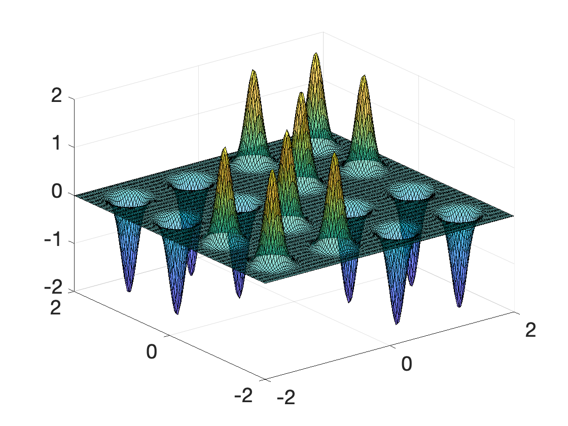
Figure 1: Left: Plot of the density $\rho_{d}$ for $d=1$ with $\sigma=0.1$. Center: Plot of the density $\rho_{d}$ for $d=2$ with $\sigma=0.1$. Right: Plot of the measure of $\pi_{d}$ for $d=1$. Arrows denote Dirac delta functions; their length and sign denote the signed mass allocated at each position.

3.1 Upper bound for two-layer discriminators

In this subsection we provide an upper bound on the two-layer IPM $d_{\mathcal{F}_{2L}}(\mu_{d},\nu_{d})$ that decreases exponentially with the dimension $d$, via a Fourier-based argument.

The Fourier transform of $\rho_{d}$.

Let $\pi_{d}=\frac{2}{4^{d}}\sum_{\beta\in\mathcal{B}^{d}}\prod_{i=1}^{d}\chi_{\beta_{i}}\delta_{\beta}=2\bigotimes_{i=1}^{d}(\frac{1}{4}\sum_{\beta_{i}\in\mathcal{B}}\chi_{\beta_{i}}\delta_{\beta_{i}})$, where $\delta_{x}$ denotes the Dirac delta at the point $x$. Formally, $\pi_{d}$ is a tempered distribution. Let $g_{d}$ be the density of the $d$-variate Gaussian $\mathcal{N}(0,\sigma^{2}\text{Id})$. The following lemma, proved in App. B, writes the density $\rho_{d}$ in terms of $\pi_{d}$ and $g_{d}$.

Lemma 1.

We can write $\rho_{d}$ as a convolution of the tempered distribution $\pi_{d}$ with the Schwartz function $g_{d}$. That is, $\rho_{d}=\pi_{d}*g_{d}$.

Thus, we have that $\widehat{\rho_{d}}=\widehat{\pi_{d}*g_{d}}=(2\pi)^{d/2}\widehat{\pi_{d}}\cdot\widehat{g_{d}}$. It is known [Bateman and Erdélyi, 1954, Kammler, 2000] that the (unitary, angular-frequency) Fourier transform of $g_{d}(x)=\frac{1}{(2\pi\sigma^{2})^{d/2}}e^{-\frac{\|y\|^{2}}{2\sigma^{2}}}$ is $\widehat{g_{d}}(\omega)=\frac{1}{(2\pi)^{d/2}}e^{-\frac{\sigma^{2}\|\omega\|^{2}}{2}}$. Also, since the Fourier transform of $x\mapsto\sin(kx)$ is $\omega\mapsto\sqrt{2\pi}\frac{\delta(\omega-k)-\delta(\omega+k)}{2i}$, we have that the Fourier transform of $x\mapsto\frac{\delta(x-k)-\delta(x+k)}{4}$ is $\omega\mapsto-\frac{i}{2\sqrt{2\pi}}\sin(k\omega)$. Thus,

$$\widehat{\pi_{d}}(\omega) =2\prod_{i=1}^{d}\bigg{(}\widehat{\frac{1}{4}\sum_{\beta_{i}\in\mathcal{B}}\chi_{\beta_{i}}\delta_{\beta_{i}}}\bigg{)}(\omega_{i})=2\prod_{i=1}^{d}\left(\frac{-i}{2\sqrt{2\pi}}\left(\sin\left(\frac{\omega_{i}}{2}\right)+\sin\left(\frac{3\omega_{i}}{2}\right)\right)\right)$$ (10)

$$=2\left(\frac{-i}{\sqrt{2\pi}}\right)^{d}\prod_{i=1}^{d}\cos\left(\omega_{i}\right)\sin\left(2\omega_{i}\right),$$ (11)

where the last equality follows from the identity $\sin(\alpha)+\sin(\beta)=2\sin(\frac{\alpha+\beta}{2})\cos(\frac{\alpha-\beta}{2})$. Consequently,

$$\widehat{\rho_{d}}(\omega)=2\left(\frac{-i}{\sqrt{2\pi}}\right)^{d}\prod_{i=1}^{d}e^{-\frac{\sigma^{2}\omega_{i}^{2}}{2}}\cos\left(\omega_{i}\right)\sin\left(2\omega_{i}\right).$$ (12)

Expressing $\mathbb{E}_{x\sim\mu_{d}}[\sigma(\langle\theta,x\rangle-b)]-\mathbb{E}_{x\sim\nu_{d}}[\sigma(\langle\theta,x\rangle-b)]$ in terms of $\widehat{\rho_{d}}$.

Note that $\mathbb{E}_{x\sim\mu_{d}}[\sigma(\langle\theta,x\rangle-b)]-\mathbb{E}_{x\sim\nu_{d}}[\sigma(\langle\theta,x\rangle-b)]$ is equal to $\int_{\mathbb{R}^{d}}\sigma(\langle\theta,x\rangle-b)\rho_{d}(x)\,dx$, for any $(\omega,b)\in\mathbb{S}^{d-1}\times\mathbb{R}$. The following proposition, which is proved in App. B and based on Lemma 3 of Domingo-Enrich and Mroueh [2021], may be used to reexpress this in terms of $\widehat{\rho_{d}}$.

Proposition 1.

Take $(\theta,b)\in\mathbb{S}^{d-1}\times\mathbb{R}$ arbitrary. For any $\varphi\in\mathcal{S}(\mathbb{R}^{d})$ and any activation $\varphi:\mathbb{R}\to\mathbb{R}$ belonging to the space of tempered distributions $\mathcal{S}(\mathbb{R})$. Then, we have

$$\int_{\mathbb{R}^{d}}\varphi(x)\sigma(\langle\theta,x\rangle-b)\,dx=(2\pi)^{(d-1)/2}\langle\hat{\sigma}(t),\hat{\varphi}(-t\theta)e^{-itb}\rangle.$$ (13)

An application of 1 yields $\int_{\mathbb{R}^{d}}\rho_{d}(x)\sigma(\langle\theta,x\rangle-b)\,dx=(2\pi)^{(d-1)/2}\langle\hat{\sigma}(t),\widehat{\rho_{d}}(-t\theta)e^{-itb}\rangle.$ Note that

$$(2\pi)^{(d-1)/2}\widehat{\rho_{d}}(-t\theta)e^{-itb}=-\sqrt{\frac{2}{\pi}}\left(-i\right)^{d}e^{-\frac{\sigma^{2}t^{2}}{2}+itb}\prod_{i=1}^{d}\cos(t\theta_{i})\sin(2t\theta_{i})$$ (14)

The following lemma provides the expressions of the Fourier transforms $\hat{\sigma}$ of the ReLU and leaky ReLU activations, as tempered distributions on $\mathbb{R}$.

Lemma 2 (Domingo-Enrich and Mroueh [2021], App. B).

Take $\sigma:\mathbb{R}\to\mathbb{R}$ of the form $\sigma(x)=c_{+}(x)_{+}^{\alpha}+c_{-}(-x)_{+}^{\alpha}$, where $c_{+},c_{-}\in\mathbb{R}$ and $\alpha\in\mathbb{Z}^{+}$. For $\alpha=1$, $c_{+}=1$, $c_{-}=0$ corresponds to the ReLU, and $c_{+}=1$, $c_{-}\in(-1,0)$ corresponds to the leaky ReLU. Then,

$$\hat{\sigma}(\omega)=A\frac{d^{\alpha}}{d\omega^{\alpha}}\left(\text{p.v.}\left[\frac{1}{i\pi\omega}\right]\right)+B\frac{d^{\alpha}}{d\omega^{\alpha}}\delta(\omega),$$ (15)

where $A=i^{\alpha-1}\frac{\alpha!}{\sqrt{2\pi}}(c_{+}-(-1)^{\alpha}c_{-})$ and $B=i^{\alpha}\sqrt{\frac{\pi}{2}}(c_{+}-(-1)^{\alpha}c_{-})+(-i)^{\alpha}c_{-}$.

Here $\text{p.v.}\left[\frac{1}{\omega}\right]$ is a Cauchy principal value, defined as $\text{p.v.}\left[\frac{1}{\omega}\right](\varphi)=\lim_{\epsilon\to 0}\int_{\mathbb{R}\setminus[-\epsilon,\epsilon]}\frac{1}{\omega}\varphi(\omega)\,d\omega=\int_{0}^{+\infty}\frac{\varphi(\omega)-\varphi(-\omega)}{\omega}$. Moreover, the derivative of a tempered distribution $f\in\mathcal{S}^{\prime}(\mathbb{R})$ is defined in the weak sense: $\langle\frac{df}{d\omega},\varphi\rangle=-\langle f,\frac{d\varphi}{d\omega}\rangle$. Applying 2 with $\alpha=1$ on equation (14), we have that

$$\int_{\mathbb{R}^{d}}\rho_{d}(x)\sigma(\langle\theta,x\rangle-b)\,dx=(2\pi)^{(d-1)/2}\langle\hat{\sigma}(t),\widehat{\rho_{d}}(-t\theta)e^{-itb}\rangle$$ (16)

$$=-\sqrt{\frac{2}{\pi}}\left(-i\right)^{d}\int_{\mathbb{R}}\left(A\frac{d}{dt}\left(\text{p.v.}\left[\frac{1}{i\pi t}\right]\right)+B\frac{d}{dt}\delta(t)\right)\left(e^{-\frac{\sigma^{2}t^{2}}{2}-itb}\prod_{i=1}^{d}\cos(t\theta_{i})\sin(2t\theta_{i})\right)\,dt$$ (17)

We can compute this explicitly. First,

$$\int_{\mathbb{R}}\frac{d}{dt}\delta(t)\left(e^{-\frac{\sigma^{2}t^{2}}{2}-itb}\prod_{i=1}^{d}\cos(t\theta_{i})\sin(2t\theta_{i})\right)\,dt=-\frac{d}{dt}\left(e^{-\frac{\sigma^{2}t^{2}}{2}-itb}\prod_{i=1}^{d}\cos(t\theta_{i})\sin(2t\theta_{i})\right)\bigg{\rvert}_{t=0}=0,$$ (18)

which holds because the factors $\sin(2t\theta_{i})$ are equal to 0 when $t=0$. Second,

$$\begin{split}&\int_{\mathbb{R}}\frac{d}{dt}\left(\text{p.v.}\left[\frac{1}{i\pi t}\right]\right)\left(e^{-\frac{\sigma^{2}t^{2}}{2}-itb}\prod_{i=1}^{d}\cos(t\theta_{i})\sin(2t\theta_{i})\right)\,dt\\ &=-\text{p.v.}\left[\frac{1}{i\pi t}\right]\left(\frac{d}{dt}\left(e^{-\frac{\sigma^{2}t^{2}}{2}-itb}\prod_{i=1}^{d}\cos(t\theta_{i})\sin(2t\theta_{i})\right)\right)\end{split}$$ (19)

The following lemma, proved in App. B, provides an upper bound strategy for Cauchy principal values:

Lemma 3.

For any $\delta>0$, $|\text{p.v.}[\frac{1}{x}](u)|\leq 2\left(\sup_{x\in(-1,1)}|u^{\prime}(x)|+\frac{1}{\delta}\sup_{x\in\mathbb{R}\setminus[-1,1]}|u(x)\cdot x^{\delta}|\right)$.

Let us set

$$\begin{split}u(t)&=\frac{d}{dt}\left(e^{-\frac{\sigma^{2}t^{2}}{2}-itb}\prod_{i=1}^{d}\cos(t\theta_{i})\sin(2t\theta_{i})\right)\\ &=\left(-\sigma^{2}t-ib-\sum_{i=1}^{d}\frac{\theta_{i}\sin(t\theta_{i})}{\cos(t\theta_{i})}+2\sum_{i=1}^{d}\frac{\theta_{i}\cos(2t\theta_{i})}{\sin(2t\theta_{i})}\right)e^{-\frac{\sigma^{2}t^{2}}{2}-itb}\prod_{i=1}^{d}\cos(t\theta_{i})\sin(2t\theta_{i}).\end{split}$$ (20)

For ease of computation, in the last equality we introduced some removable singularities. 9 in App. B provides the following bounds:

$$\sup_{x\in\mathbb{R}}|u^{\prime}(x)|\leq O\left(\kappa^{d}\left(d^{2}+d|b|+b^{2}\right)\right),\text{ and }\sup_{x\in\mathbb{R}}|u(x)\cdot x^{\delta}|\leq O\left(\kappa^{d}\left(\frac{d+|b|}{\sigma}\right)\right).$$ (21)

The key idea of the proof of 9 (and of the whole construction in this section) is the inequality $\sup_{t\in\mathbb{R}}|\prod_{i=1}^{d}\cos(t\theta_{i})\sin(2t\theta_{i})|\leq\kappa^{d}$, where $\kappa:=\sup_{x\in\mathbb{R}}|\cos(t)\sin(2t)|=0.7698\dots$ (see Figure 4). Since $\kappa<1$, the factor $|\prod_{i=1}^{d}\cos(t\theta_{i})\sin(2t\theta_{i})|$ is exponentially small in the dimension $d$.

Plugging the bounds (21) into 3 yields an upper bound on the absolute value of (LABEL:eq:pv_computation). In consequence, the following upper bound holds:

Proposition 2.

We have $\left|\int_{\mathbb{R}^{d}}\rho_{d}(x)\sigma(\langle\theta,x\rangle-b)\,dx\right|\leq O\left(\kappa^{d}\left(d^{2}+d|b|+b^{2}+\frac{d+|b|}{\sigma}\right)\right)$ for any $(\theta,b)\in\mathbb{S}^{d-1}\times\mathbb{R}$.

Concluding the upper bound.

2 shows that if $|b|\leq d+\sqrt{d}$, then we can write $\left|\int_{\mathbb{R}^{d}}\rho_{d}(x)\sigma(\langle\theta,x\rangle-b)\,dx\right|\leq O\left(\kappa^{d}\left(d^{2}+\frac{d}{\sigma}\right)\right).$ That is, unless $|b|$ is large, $\left|\int_{\mathbb{R}^{d}}\rho_{d}(x)\sigma(\langle\theta,x\rangle-b)\,dx\right|$ decreases exponentially with the dimension $d$. In the following, we show that for large $d$, this is also the case. Namely,

Lemma 4.

If $|b|>d+\sqrt{d}$, then $\left|\int_{\mathbb{R}^{d}}\rho_{d}(x)\sigma(\langle\theta,x\rangle-b)\,dx\right|\leq\frac{\sigma}{\sqrt{2\pi}}e^{-\frac{d^{2}}{2\sigma^{2}}}$.

4, which is proved in App. B, allows us to conclude the upper bound.

Theorem 3.

The following inequality holds for the IPM between $\mu_{d}$ and $\nu_{d}$ corresponding to the class $\mathcal{F}_{2L}$ of two-layer networks:

$$d_{\mathcal{F}_{2L}}(\mu_{d},\nu_{d})=\sup_{(\theta,b)\in\mathbb{S}^{d-1}}\left|\int_{\mathbb{R}^{d}}\rho_{d}(x)\sigma(\langle\theta,x\rangle-b)\,dx\right|\leq O\left(\max\left\{\kappa^{d}\left(d^{2}+\frac{d}{\sigma}\right),\sigma e^{-\frac{d^{2}}{2\sigma^{2}}}\right\}\right).$$ (22)

3.2 Lower bound for three-layer discriminators.

In order to provide a lower bound on the IPM $d_{\mathcal{F}_{3L}}(\mu_{d},\nu_{d})$ we construct a specific three-layer network $F$, and then show a lower bound on $|\mathbb{E}_{x\sim\mu_{d}}[F(x)]-\mathbb{E}_{x\sim\nu_{d}}[F(x)]|$ and an upper bound on the path-norm of $F$.

Construction of the discriminator $F$.

Let us fix $0<x_{0}<1/4$ arbitrary. Define the two-layer network $f_{1}:\mathbb{R}\to\mathbb{R}$ as

$$f_{1}(x)=\sum_{\beta\in\mathcal{B}}\frac{\text{sign}(\beta)}{x_{0}}\left((x-(\beta-2x_{0}))_{+}-(x-(\beta-x_{0}))_{+}-(\beta-(b+x_{0}))_{+}+(x-(\beta+2x_{0}))_{+}\right)$$ (23)

The function $f_{1}$, which is plotted in Figure 2 (left), takes non-zero values only around points in $\mathcal{B}$, and it takes value 1 around positive $\beta\in\mathcal{B}$, and value -1 around negative $\beta\in\mathcal{B}$.

If $d$ is even, we define the two-layer network $f_{2}:\mathbb{R}\to\mathbb{R}$ as

$$\begin{split}f_{2}(x)&=1-(x)_{+}-(-x)_{+}-(-1)^{d/2}((x-d)_{+}+(-x-d)_{+})\\ &-2\sum_{i=1}^{(d-2)/2}(-1)^{i}((x-2i)_{+}+(-x-2i)_{+}).\end{split}$$ (24)

This function is plotted for $d=4$ in Figure 2 (center), and it takes alternating values $\pm 1$ at even integers. If $d\geq 3$ is odd, we define $f_{2}$ as

$$\begin{split}f_{2}(x)&=x+(-1)^{(d-1)/2}(-(x-d)_{+}+(-x-d)_{+})\\ &+2\sum_{i=0}^{(d-3)/2}(-1)^{i}(-(x-2i-1)_{+}+(-x-2i-1)_{+}).\end{split}$$ (25)

This function is plotted for $d=5$ in Figure 2 (right), and it takes alternating values $\pm 1$ at odd integers.

Figure 2: Left: Plot of the function $f_{1}$ defined in (23), for the value $x_{0}=0.1$. Center: Plot of the function $f_{2}$ for $d=4$ (defined in (24)). Right: Plot of the function $f_{2}$ for $d=5$ (defined in (25)).

We define the discriminator $F:\mathbb{R}^{d}\to\mathbb{R}$ as

$$F(x)=f_{2}\bigg{(}\sum_{i=1}^{d}f_{1}(x_{i})\bigg{)}.$$ (26)

Construction of random variables $Z^{+},Z^{-}$ with distributions $\mu_{d},\nu_{d}$.

If $\xi^{+},\xi^{-}$ are random vectors distributed uniformly over $\mathcal{B}^{d}_{+}$ and $\mathcal{B}^{d}_{-}$ respectively, and $X$ is a $d$-variate Gaussian $\mathcal{N}(0,\sigma^{2}\text{Id})$, the variables $Z^{+}=\xi^{+}+X$ and $Z^{-}=\xi^{-}+X$ are distributed according to $\mu_{d}$ and $\nu_{d}$ respectively. To see this, note that in analogy with $\rho_{d}=\pi_{d}*g_{d}$, we can write $\rho_{d}^{\pm}=\pi_{d}^{\pm}*g_{d}$, where $\pi_{d}^{\pm}=\frac{2}{4^{d}}\sum_{\beta\in\mathcal{B}^{d}_{\pm}}\prod_{i=1}^{d}\chi_{\beta_{i}}\delta_{\beta}$. Since $\xi^{\pm}$ are distributed according to $\pi^{\pm}_{d}$, and the law of a sum of random variables is the convolution of their distributions, the result follows. Thus, we can reexpress $\int_{\mathbb{R}^{d}}F(x)\,d(\mu_{d}-\nu_{d})(x)$ as $\mathbb{E}[F(Z^{+})]-\mathbb{E}[F(Z^{-})]$.

Lower-bounding $\mathbb{E}[F(Z^{+})]-\mathbb{E}[F(Z^{-})]$.

At this point, we take an arbitrary $0<\epsilon<1$, and define the sequence $(\sigma_{d})_{d\geq 0}$ as the solutions of $\frac{x_{0}^{2}}{2\sigma_{d}^{2}}=\log(\frac{d\sigma_{d}}{\sqrt{2\pi}\epsilon x_{0}})$. The solution $\sigma_{d}$ exists and is unique because the function $\sigma\mapsto\frac{x_{0}^{2}}{2\sigma^{2}}$ is strictly decreasing and bijective from $(0,+\infty)$ to $(0,+\infty)$, while the function $\sigma\mapsto\log(\frac{d\sigma}{\sqrt{2\pi}\epsilon x_{0}})$ is strictly increasing and bijective from $(0,\infty)$ to $\mathbb{R}$. The following result regarding the sequence $(\sigma_{d})_{d}$ is shown in App. B.

Lemma 5.

If $(X_{i})_{i=1}^{d}$ are independent random variables with distribution $\mathcal{N}(0,\sigma_{d}^{2})$, we have that $P(\forall i\in\{1,\dots,d\},\,X_{i}\leq x_{0})\geq 1-\epsilon$. The sequence $(\sigma_{d})_{d}$ is strictly decreasing, and $\sigma_{d}=\Omega(1/\log(d))$.

This allows us to prove an instrumental proposition concerning the values of $F$ at $Z^{+}$ and $Z^{-}$.

Proposition 3.

With probability at least $1-2\epsilon$, we have that simultaneously,

$$\begin{split}F(Z^{+})=1\quad\text{and}\quad F(Z^{-})=-1,\quad\text{when }d\equiv 0,1\,(\text{mod }4)\\ F(Z^{+})=-1\quad\text{and}\quad F(Z^{-})=1,\quad\text{when }d\equiv 2,3\,(\text{mod }4)\end{split}$$ (27)

Consequently, $\left|\mathbb{E}\left[F(Z^{+})\right]-\mathbb{E}\left[F(Z^{-})\right]\right|\geq 2-8\epsilon$.

Proof sketch. By 5, with probability at least $1-2\epsilon$, $|X_{i}|\leq x_{0}$ for all $i\in\{1,\dots,d\}$. Equivalently, $|Z^{+}_{i}-\xi^{+}_{i}|\leq x_{0}$ and $|Z^{-}_{i}-\xi^{-}_{i}|\leq x_{0}$ for all $i\in\{1,\dots,d\}$. This implies that $f_{1}(Z^{+}_{i})=\text{sign}(Z^{+}_{i})=\text{sign}(\xi^{+}_{i})$ and $f_{1}(Z^{-}_{i})=\text{sign}(Z^{-}_{i})=\text{sign}(\xi^{-}_{i})$ for all $i\in\{1,\dots,d\}$. The statements (27) follow from the definitions of the functions $f_{2}$ and the lower bound is a consequence of (27) and the boundedness of $|F|$ (see full proof in App. B). ∎

Bounding the path-norm of the discriminator $F$.

The following lemma, proved in App. B, characterizes the discriminator $F$ as a three-layer network and provides bounds on its path-norms.

Lemma 6.

The function $F$ defined in (26) can be expressed as a three-layer ReLU neural network $f_{\mathcal{W}}$ of the form (1) with widths $m_{1}=16d$ and $m_{2}=d+2$, with path-norms

$$\begin{split}&\text{PN}_{b}(\mathcal{W})\leq\bigg{(}\frac{64}{x_{0}}+1\bigg{)}d^{2}+1\text{ for $d$ even, and }\text{PN}_{b}(\mathcal{W})\leq\bigg{(}\frac{64}{x_{0}}+1\bigg{)}d^{2}+\frac{64d}{x_{0}}+2\text{ for $d$ odd.}\\ &\text{PN}_{nb}(\mathcal{W})=\frac{32d^{2}}{x_{0}}\text{ for $d$ even, and }\text{PN}_{nb}(\mathcal{W})=\frac{32d^{2}+32d}{x_{0}}\text{ for $d$ odd.}\end{split}$$ (28)

We are in position to state the formal version of Theorem 1.

Theorem 4.

Setting $\epsilon=1/8$ and $x_{0}=1/8$, we obtain that

$$d_{\mathcal{F}_{2L}}(\mu_{d},\nu_{d}) =O(\kappa^{d}d^{2}),$$ (29)

$$d_{\mathcal{F}_{3L}}(\mu_{d},\nu_{d}) \geq\frac{1}{513d^{2}+512d+1}.$$ (30)

Proof.

To prove (29), we plugged the bound $\sigma_{d}=\Omega(1/\log(d))$ from 5 into Theorem 3. We also used that for $\epsilon=1/8$ and $x_{0}=1/8$, $\sigma_{d}\leq 1/6$ because at $1/6$, the curve $\sigma\mapsto\frac{x_{0}^{2}}{2\sigma^{2}}$ is below $\sigma\mapsto\log(\frac{d\sigma}{\sqrt{2\pi}\epsilon x_{0}})$. Hence, $\sigma e^{-\frac{d^{2}}{2\sigma^{2}}}=O(\log(d)e^{-18d^{2}}),$ which is $O(\kappa^{d}d^{2})$. To prove (30), we use that by 3, $F$ is a three-layer neural network such that $|\mathbb{E}_{x\sim\mu_{d}}[F(x)]-\mathbb{E}_{x\sim\nu_{d}}[F(x)]|\geq 1$, and with path-norm with bias bounded by $513d^{2}+512d+1$. Dividing the outermost layer weights by this quantity, we obtain a three-layer network with unit path-norm and the result follows. ∎

Note that if we consider the discriminator class of three-layer networks with bounded path-norm without bias, 6 gives a lower bound of order $\Omega(1/d^{2})$ as well.

4 Separation between two-layer and RKHS discriminators

The pair $(\mu_{d},\nu_{d})$.

For any $d\geq 0$, we define a pair of measures $\mu_{d},\nu_{d}\in\mathcal{P}(\mathbb{R}^{d})$ with densities $\frac{d\mu_{d}}{dx}=\rho^{+}_{d}$, $\frac{d\nu_{d}}{dx}=\rho^{+}_{d}$ such that

$$\rho_{d}(x):=\frac{2\sigma^{d}}{(2\pi)^{d/2}}e^{-\frac{\sigma^{2}\|x\|^{2}}{2}}\sin\left(\ell x_{1}\right),\quad\text{where }x_{1}=\langle x,e_{1}\rangle.$$ (31)

Since $\int_{\mathbb{R}^{d}}\rho_{d}(x)\,dx=0$ because $\rho_{d}$ is odd with respect to $x_{1}$, and $\int_{\mathbb{R}^{d}}|\rho_{d}(x)|\,dx\leq\frac{2\sigma^{d}}{(2\pi)^{d/2}}\int_{\mathbb{R}^{d}}e^{-\frac{\sigma^{2}\|x\|^{2}}{2}}\,dx=2$, we have freedom in specifying $\rho^{+}_{d},\rho^{-}_{d}$. If $\xi$ is the density of an arbitrary probability measure on $\mathbb{R}^{d}$, setting $\rho^{+}_{d}(x)=(1-\frac{1}{2}\int_{\mathbb{R}^{d}}|\rho_{d}(x)|\,dx)\xi(x)+\max\{0,\rho_{d}(x)\}$ and $\rho^{-}_{d}(x)=(1-\frac{1}{2}\int_{\mathbb{R}^{d}}|\rho_{d}(x)|\,dx)\xi(x)+\max\{0,-\rho_{d}(x)\}$ works. Figure 1 shows plots of $\rho_{d}$ for $d=1,2$.

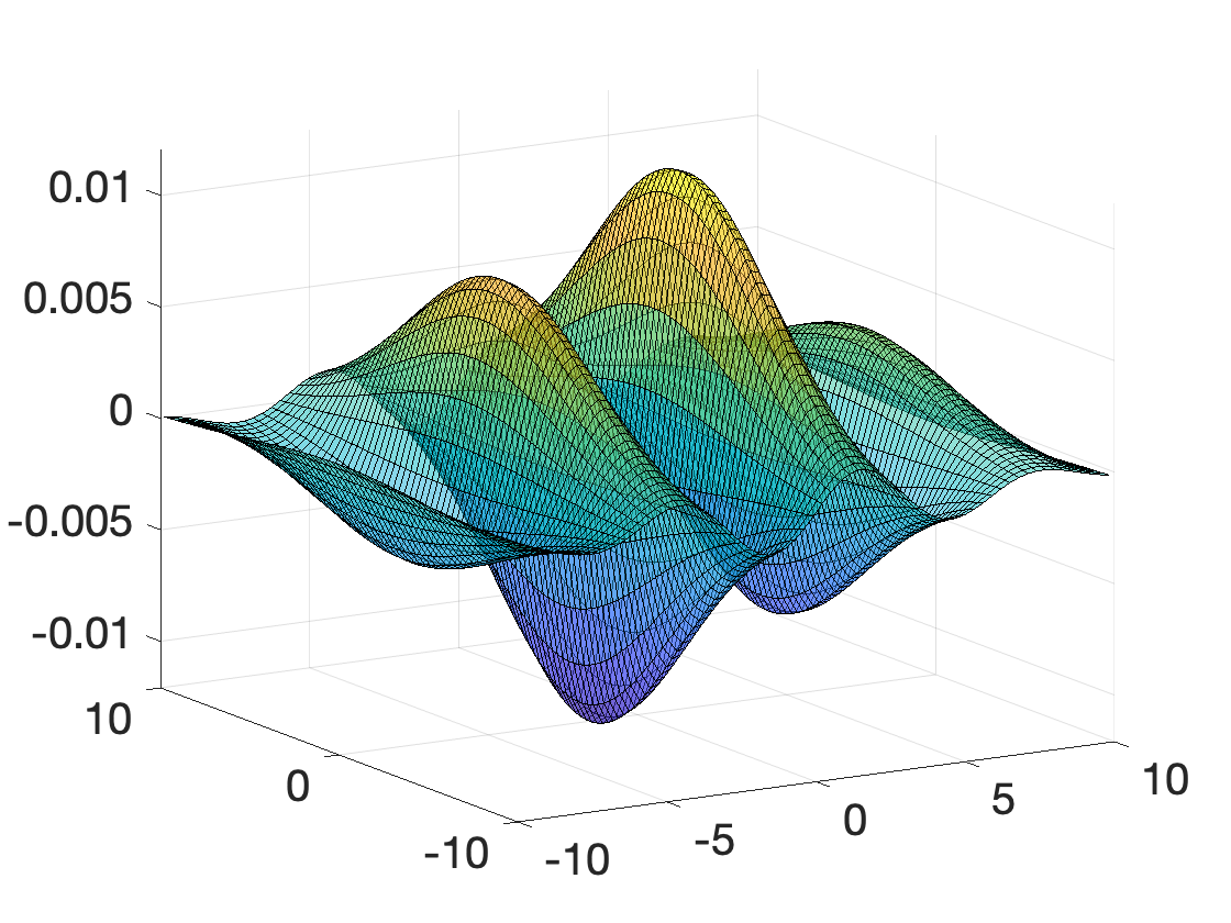
Figure 3: Left: Plot of the density $\rho_{d}$ for $d=1$ with $\sigma=0.2$ and $\ell=1$. Right: Plot of the density $\rho_{d}$ for $d=2$ with $\sigma=0.2$ and $\ell=1$.

The following lemma provides the Fourier transform of $\rho_{d}$. The proof in App. C involves using the convolution theorem; in this case $\rho_{d}$ is expressed as a product of functions and $\hat{\rho}_{d}$ is proportional to the convolution of their Fourier transforms.

Lemma 7.

The Fourier transform of $\rho_{d}$ reads $\widehat{\rho_{d}}(x)=\frac{i}{(2\pi)^{d/2}}(e^{-\frac{\|x+\ell e_{1}\|^{2}}{2\sigma^{2}}}-e^{-\frac{\|x-\ell e_{1}\|^{2}}{2\sigma^{2}}})$.

As in Sec. 3, an application of 1 shows that $\int_{\mathbb{R}^{d}}\rho_{d}(x)\sigma(\langle\theta,x\rangle-b)\,dx$ is equal to $(2\pi)^{(d-1)/2}\langle\hat{\sigma}(t),\widehat{\rho_{d}}(-t\theta)e^{-itb}\rangle$. Analogously, we use the expression of $\hat{\sigma}$ for the ReLU-like activations provided by 2, and we obtain an explicit expression for $\int_{\mathbb{R}^{d}}\rho_{d}(x)\sigma(\langle\theta,x\rangle-b)\,dx$ from which the upper and lower bounds will follow:

$$\frac{i}{\sqrt{2\pi}}\int_{\mathbb{R}}\left(A\frac{d^{\alpha}}{dt^{\alpha}}\left(\text{p.v.}\left[\frac{1}{i\pi t}\right]\right)+B\frac{d^{\alpha}}{dt^{\alpha}}\delta(t)\right)\left(\left(e^{-\frac{\|t\theta-\ell e_{1}\|^{2}}{2\sigma^{2}}}-e^{-\frac{\|t\theta+\ell e_{1}\|^{2}}{2\sigma^{2}}}\right)e^{-itb}\right)\,dt,$$ (32)

which can be simplified to (see 13 in App. C):

$$\sqrt{\frac{2}{\pi}}i\left(-\frac{A\ell\theta_{1}}{\sigma^{2}}e^{-\frac{\ell^{2}}{2\sigma^{2}}}+B\int_{0}^{+\infty}\frac{\sin(tb)(\exp(-\frac{\|t\theta-\ell e_{1}\|^{2}}{2\sigma^{2}})-\exp(-\frac{\|t\theta+\ell e_{1}\|^{2}}{2\sigma^{2}}))}{t^{2}}\,dt\right)$$ (33)

Upper bound for RKHS discriminators.

By equation (7), the IPM $d_{\mathcal{F}_{\mathcal{H}}}(\mu_{d},\nu_{d})$ corresponding to the unit ball of the RKHS $\mathcal{H}$ takes the form $(\int_{\mathbb{S}^{d-1}\times\mathbb{R}}(\int_{\mathbb{R}^{d}}\sigma\left(\langle\theta,x\rangle-b\right)\rho_{d}(x)\,dx)^{2}\,d\tau(\theta,b))^{1/2}$. Armed with the expression (33) for $\int_{\mathbb{R}^{d}}\sigma\left(\langle\theta,x\rangle-b\right)\rho_{d}(x)\,dx$, we proceed to upper-bound the absolute value of this expression in the following proposition proved in App. C.

Proposition 4.

We have that

$$d_{\mathcal{F}_{\mathcal{H}}}(\mu_{d},\nu_{d})=O\left(d^{1/4}\left(\frac{1}{2^{d/4}}+e^{-\frac{\ell^{2}}{4\sigma^{2}}}\right)+\frac{\ell^{2}}{\sigma^{4}}e^{-\frac{(\ell-1)^{2}}{2\sigma^{2}}}+\left(\frac{\ell}{\sigma^{2}}+1\right)e^{-\frac{\ell^{2}}{2\sigma^{2}}}\right).$$ (34)

Evidently, the upper bound depends on the choices of the parameters $\ell$ and $\sigma$ as a function of $d$.

Lower bound for two-layer discriminators.

Our approach to lower-bound the IPM $d_{\mathcal{F}_{2L}}(\mu_{d},\nu_{d})$ is to lower-bound $\int_{\mathbb{R}^{d}}\rho_{d}(x)\sigma(\langle\theta,x\rangle-b)\,dx$ for some well chosen $(\theta,b)\in\mathbb{S}^{d-1}\times\mathbb{R}$, via the expression (33). The result is as follows:

Proposition 5.

Define the ${(\ell_{d})}_{d\geq 0}$ as $\ell_{d}=\sqrt{d}$ and ${(\sigma_{d})}_{d\geq 0}$ as the sequence of solutions to $\frac{x_{0}^{2}}{2\sigma^{2}}=\log\left(\frac{\sqrt{2}d^{2}\sigma}{\sqrt{\pi}x_{0}}\right)$, which fulfills $\sigma_{d}\geq K/\log(d)$. Then, $d_{\mathcal{F}_{2L}}(\mu_{d},\nu_{d})=\Omega\left(\frac{1}{d\log(d)}\right)$.

If we substitute the choices we made for $(\ell_{d})$ and $(\sigma_{d})$ into (34), we obtain

$$d_{\mathcal{F}_{\mathcal{H}}}(\mu_{d},\nu_{d})=O\bigg{(}d^{1/4}\left(\frac{1}{2^{d/4}}+e^{-\frac{d}{16}}\right)+\frac{de^{-\frac{(\sqrt{d}-1)^{2}}{16}}}{16}+\frac{\sqrt{d}+4}{4}e^{-\frac{d}{8}}\bigg{)}=O\bigg{(}de^{-\frac{(\sqrt{d}-1)^{2}}{16}}\bigg{)},$$ (35)

which yields Theorem 2.

5 Discussion

Why small IPM values preclude discrimination of distributions from samples.

Suppose that $\mathcal{F}$ is a class of functions $\mathbb{R}^{d}\to\mathbb{R}$, and $\mu_{n},\nu_{n}$ are empirical measures built from $n$ samples from $\mu,\nu$ respectively. Let $\hat{\mathcal{F}}_{\mu}=\{f-\mathbb{E}_{x\sim\mu}[f(x)]\,|\,f\in\mathcal{F}\}$ be the recentered function class according to $\mu$ (analogous for $\nu$). Letting $\mathcal{R}_{n}(\mathcal{F})=\mathbb{E}_{\sigma_{i},x_{i}}\sup_{f\in\mathcal{F}}|\frac{1}{n}\sum_{i=1}^{n}\sigma_{i}f(x_{i})|$ be the Rademacher complexity of $\mathcal{F}$, it turns out that $\frac{1}{2}\mathcal{R}_{n}(\hat{\mathcal{F}}_{\mu})\leq\mathbb{E}[\sup_{f\in\mathcal{F}}|\mathbb{E}_{x\sim\mu}[f(x)]-\mathbb{E}_{x\sim\mu_{n}}[f(x)]|]\leq 2\mathcal{R}(\mathcal{F})$ (Proposition 4.11, Wainwright [2019]), and an application of McDiarmid’s inequality shows that w.h.p. (with high probability), the IPM $d_{\mathcal{F}}(\mu,\mu_{n})=\sup_{f\in\mathcal{F}}|\mathbb{E}_{x\sim\mu}[f(x)]-\mathbb{E}_{x\sim\mu_{n}}[f(x)]|$ does not lie far from these bounds.

$\mathcal{F}$ is a useful discriminator class if $d_{\mathcal{F}}(\mu_{n},\nu_{n})$ is informative of the value of $d_{\mathcal{F}}(\mu,\nu)$ for a tractable data size $n$. This is not the case if $d_{\mathcal{F}}(\mu,\nu)$ is negligible compared to $d_{\mathcal{F}}(\mu,\mu_{n}),d_{\mathcal{F}}(\nu,\nu_{n})$ and their fluctuations, as the statistical noise dominates over the signal. Since $d_{\mathcal{F}}(\mu,\mu_{n}),d_{\mathcal{F}}(\nu,\nu_{n})$ are w.h.p. of the order of $\frac{1}{2}\mathcal{R}_{n}(\hat{\mathcal{F}}_{\mu})$, and the classes $\mathcal{F}_{3L},\mathcal{F}_{2L},\mathcal{F}_{\mathcal{H}}$ studied in our paper (as well as their centered versions) have Rademacher complexities $\Theta(1/\sqrt{n})$ [E and Wojtowytsch, 2020], we need to take $n$ of order $\Omega(1/d_{\mathcal{F}}(\mu,\nu)^{2})$ to get decent discriminator performance. The required $n$ is prohibitively costly when $d_{\mathcal{F}}(\mu_{d},\nu_{d})$ is exponentially small in $d$, as in our cases.

Can we make $\mu_{d}$ and $\nu_{d}$ any simpler in Sec. 3?

One might wonder whether a simpler $\rho_{d}$ might suffice to show a separation result. Specifically, one might think of replacing $\mathcal{B}=\{\pm\frac{3}{2},\pm\frac{1}{2}\}$ by $\mathcal{B}=\{\pm 1\}$. The upper bound on two-layer networks would not go through because the factor $\prod_{i=1}^{d}\cos\left(\omega_{i}\right)\sin\left(2\omega_{i}\right)$ would become $\prod_{i=1}^{d}\sin\left(\omega_{i}\right)$, which does not admit a uniform exponentially decreasing upper bound. Moreover, it can be seen that for $\sigma=O(1/\log(d))$, the two-layer network $f_{2}(\sum_{i=1}^{d}x_{i})$ would be able to discriminate between $\mu_{d}$ and $\nu_{d}$.

Do our arguments work for other activation functions and weight norms?

Our proofs makes use of the specific form of the Fourier transform of the ReLU and leaky ReLU. One may try to apply the same method for other activation functions via their Fourier transforms; intuitively one should be able to obtain exponentially decreasing lower bounds as well, because the factor $\prod_{i=1}^{d}\cos\left(\omega_{i}\right)\sin\left(2\omega_{i}\right)$ will show up in some way or another. If we use different norms to define the three-layer and two-layer IPMs, the results are unchanged up to polynomial factors because weight norms are equivalent to each other up to polynomial factors in $d$ (using that the widths of our networks are polynomial in $d$). Finally, it would be interesting to adapt our upper bound for the MMD to slightly different kernels such as the neural tangent kernel (NTK, Jacot et al. [2018]).

Appendix A IPM derivations

Define the function class $G_{3L}$ of ReLU neural networks of the form $g(x)=\pm\sigma(\sum_{j=1}^{m_{1}}w_{j}\sigma(\langle\theta_{j},x\rangle-b_{j})+w_{0})$ such that $\sum_{j=1}^{m_{1}}|w_{j}|\cdot\|(\theta_{j},b_{j})\|_{2}+|w_{0}|\leq 1$.

Lemma 8.

Any function in $F_{3L}$ may be written as a convex combination of functions in $G_{3L}$ and the constant function 1.

Proof.

Let

$$f_{\mathcal{W}}(x)=\sum_{i=1}^{m_{2}}w_{i}\sigma\left(\sum_{j=1}^{m_{1}}W_{i,j}\sigma\left(\langle\theta_{j},x\rangle-b_{j}\right)+W_{i,0}\right)+w_{0}.$$ (36)

belong to $F_{3L}$, which means that $\text{PN}_{b}(\mathcal{W})=\sum_{i=1}^{m_{2}}|w_{i}|(\sum_{j=1}^{m_{1}}|W_{i,j}|\cdot\|(\theta_{j},b_{j})\|_{2}+|W_{i,0}|)+|w_{0}|\leq 1$. We may renormalize the weights such that $\sum_{j=1}^{m_{1}}|W_{i,j}|\cdot\|(\theta_{j},b_{j})\|_{2}+|W_{i,0}|=1$ for all $i$, by moving the appropriate factors outside of the ReLU activation thanks to the 1-homogeneity. Then, $\text{PN}_{b}(\mathcal{W})=\sum_{i=0}^{m_{2}}|w_{i}|\leq 1$. We may further renormalize the weights such that $\sum_{i=0}^{m_{2}}|w_{i}|=1$ and $\sum_{j=1}^{m_{1}}|W_{i,j}|\cdot\|(\theta_{j},b_{j})\|_{2}+|W_{i,0}|\leq 1$ for all $i$.

Setting $g_{i}(x)=\text{sign}(w_{i})\sigma\left(\sum_{j=1}^{m_{1}}W_{i,j}\sigma\left(\langle\theta_{j},x\rangle-b_{j}\right)+W_{i,0}\right)$, we obtain the expression $f_{\mathcal{W}}(x)=\sum_{i=1}^{m_{2}}|w_{i}|g_{i}(x)+|w_{0}|$. That is, $f_{\mathcal{W}}$ can be written as a convex combination of $\{g_{i}\}_{i=1}^{m_{2}}$ and the constant function 1. Note that $g_{i}$ belongs to $G_{3L}$, which concludes the proof. ∎

Since $f\mapsto\pm(\mathbb{E}_{x\sim\mu}[f(x)]-\mathbb{E}_{x\sim\nu}[f(x)])$ are concave mappings, their suprema over $G_{3L}$ is equal to their suprema over the convex hull $\text{conv}(G_{3L})$. Since $\mathbb{E}_{x\sim\mu}[f(x)]-\mathbb{E}_{x\sim\nu}[f(x)]$ is 0 when $f$ is a constant function, by 8 the suprema over $\text{conv}(G_{3L})$ are equal to the suprema over $F_{3L}$, which concludes the proof of equation (5). Equation (6) follows from a similar argument. Equation (7) is derived using the proof of Lemma 2 of Domingo-Enrich and Mroueh [2021].

Appendix B Proofs of Sec. 3

Proof of 1. If we take a Schwartz function $\varphi\in\mathcal{S}(\mathbb{R}^{d})$, we have

$$\begin{split}&\langle\pi_{d}*g_{d},\varphi\rangle=\langle g_{d}(y),\langle\varphi(x+y),\pi_{d}(x)\rangle\rangle\\ &=\int_{\mathbb{R}^{d}}\frac{1}{(2\pi\sigma^{2})^{d/2}}e^{-\frac{\|y\|^{2}}{2\sigma^{2}}}\left\langle\varphi(x+y),\frac{2}{4^{d}}\sum_{\beta\in\mathcal{B}^{d}}\prod_{i=1}^{d}\chi_{\beta_{i}}\delta_{\beta}\right\rangle\,dy\\ &=\frac{2}{(4\sqrt{2\pi\sigma^{2}})^{d}}\int_{\mathbb{R}^{d}}e^{-\frac{\|y\|^{2}}{2\sigma^{2}}}\sum_{\beta\in\mathcal{B}^{d}}\prod_{i=1}^{d}\chi_{\beta_{i}}\varphi(y+\beta)\,dy\\ &=\frac{2}{(4\sqrt{2\pi\sigma^{2}})^{d}}\sum_{\beta\in\mathcal{B}^{d}}\prod_{i=1}^{d}\chi_{b_{i}}\int_{\mathbb{R}^{d}}e^{-\frac{\|y\|^{2}}{2\sigma^{2}}}\varphi(y+\beta)\,dy\\ &=\frac{2}{(4\sqrt{2\pi\sigma^{2}})^{d}}\sum_{\beta\in\mathcal{B}^{d}}\prod_{i=1}^{d}\chi_{b_{i}}\int_{\mathbb{R}^{d}}e^{-\frac{\|\tilde{y}-\beta\|^{2}}{2\sigma^{2}}}\varphi(\tilde{y})\,d\tilde{y}\\ &=\frac{2}{(4\sqrt{2\pi\sigma^{2}})^{d}}\int_{\mathbb{R}^{d}}\sum_{\beta\in\mathcal{B}^{d}}\prod_{i=1}^{d}\chi_{b_{i}}e^{-\frac{\|\tilde{y}-\beta\|^{2}}{2\sigma^{2}}}\varphi(\tilde{y})\,d\tilde{y}=\langle\rho_{d},\varphi\rangle.\end{split}$$ (37)

∎

Proof of 1. We adapt the argument of Lemma 3 of Domingo-Enrich and Mroueh [2021]. Define $\sigma_{b}:\mathbb{R}\to\mathbb{R}$ as the translation of $\sigma$ by $-b$, i.e. $\sigma_{b}(x)=\sigma(x-b)$. Note that $\widehat{\sigma_{b}}(\omega)=e^{-ib\omega}\hat{\sigma}(\omega)$. We have

$$\begin{split}&\int_{\mathbb{R}^{d}}\varphi(x)\sigma(\langle\theta,x\rangle-b)\,dx=\int_{\mathbb{R}^{d}}\varphi(x)\sigma_{b}(\langle\theta,x\rangle)\,dx=\int_{\mathbb{R}^{d}}\left(\frac{1}{(2\pi)^{d/2}}\int_{\mathbb{R}^{d}}\hat{\varphi}(\omega)e^{i\langle\omega,x\rangle}\,d\omega\right)\sigma_{b}(\langle\theta,x\rangle)\,dx\\ &=\int_{\text{span}(\theta)}\int_{\text{span}(\theta)^{\perp}}\left(\frac{1}{(2\pi)^{d/2}}\int_{\text{span}(\theta)^{\perp}}\left(\int_{\text{span}(\theta)}\hat{\varphi}(\omega)e^{i\langle\omega_{\theta},x_{\theta}\rangle}\,d\omega_{\theta}\right)e^{i\langle\omega_{\theta^{\perp}},x_{\theta^{\perp}}\rangle}\,d\omega_{\theta^{\perp}}\right)\,dx_{\theta^{\perp}}\sigma_{b}(\langle\theta,x_{\theta}\rangle)\,dx_{\theta}\\ &=\frac{1}{\sqrt{2\pi}}\int_{\text{span}(\theta)}(2\pi)^{(d-1)/2}\int_{\text{span}(\theta)}\hat{\varphi}(\omega_{\theta})e^{i\langle\omega_{\theta},x_{\theta}\rangle}\,d\omega_{\theta}\,\sigma_{b}(\langle\theta,x_{\theta}\rangle)\,dx_{\theta}\\ &=(2\pi)^{(d-1)/2}\int_{\mathbb{R}}\frac{1}{\sqrt{2\pi}}\int_{\mathbb{R}}\hat{\varphi}(t\theta)e^{itx}\,dt\,\sigma_{b}(x)\,dx=(2\pi)^{(d-1)/2}\int_{\mathbb{R}}\frac{1}{\sqrt{2\pi}}\int_{\mathbb{R}}\hat{\varphi}(t\theta)e^{itx}\,dt\,\sigma(x-b)\,dx\\ &=(2\pi)^{(d-1)/2}\int_{\mathbb{R}}\frac{1}{\sqrt{2\pi}}\int_{\mathbb{R}}\hat{\varphi}(t\theta)e^{it(\tilde{x}+b)}\,dt\,\sigma(\tilde{x})\,dx=(2\pi)^{(d-1)/2}\langle\check{\sigma}(t),\hat{\varphi}(t\theta)e^{itb}\rangle.\end{split}$$ (38)

In the third equality, we rewrite $\mathbb{R}^{d}=\text{span}(\theta)+\text{span}(\theta)^{\perp}$ and we use Fubini’s theorem twice. In the fourth equality we use the following argument: denoting $h(x_{\theta^{\perp}},\omega_{\theta})=\int_{\text{span}}\hat{\varphi}(\omega_{\theta}+\omega_{\theta}^{\perp})e^{i\langle\omega_{\theta},x_{\theta}\rangle}\,d\omega_{\theta}$, we have that

$$\begin{split}&\int_{\text{span}(\theta)^{\perp}}\left(\int_{\text{span}(\theta)^{\perp}}h(x_{\theta^{\perp}},\omega_{\theta})e^{i\langle\omega_{\theta^{\perp}},x_{\theta^{\perp}}\rangle}\,d\omega_{\theta^{\perp}}\right)dx_{\theta^{\perp}}=(2\pi)^{(d-1)/2}\int_{\text{span}(\theta)^{\perp}}\hat{h}(-\omega_{\theta^{\perp}},\omega_{\theta})\,d\omega_{\theta^{\perp}}\\ &=(2\pi)^{d-1}h(0,\omega_{x})=(2\pi)^{d-1}\int_{\text{span}(\theta)}\hat{\varphi}(\omega_{\theta})e^{i\langle\omega_{\theta},x_{\theta}\rangle}\,d\omega_{\theta}.\end{split}$$ (39)

To conclude the proof, note that for any test function $\varphi\in\mathcal{S}(\mathbb{R})$, $\langle\check{\sigma}(x),\varphi(x)\rangle=\langle\sigma(x),\check{\varphi}(x)\rangle=\int_{\mathbb{R}}\sigma(x)\frac{1}{\sqrt{2\pi}}\,\int_{\mathbb{R}}e^{itx}\varphi(t)\,dt\,dx=\int_{\mathbb{R}}\sigma(x)\frac{1}{\sqrt{2\pi}}\,\int_{\mathbb{R}}e^{-i(-t)x}\varphi(t)\,dt\,dx=\int_{\mathbb{R}}\sigma(x)\frac{1}{\sqrt{2\pi}}\,\int_{\mathbb{R}}e^{-itx}\varphi(-t)\,dt\,dx=\langle\hat{\sigma}(x),\varphi(-x)\rangle$. ∎

Proof of 3. Recall that $\text{p.v.}\left[\frac{1}{\omega}\right](u)=\int_{0}^{+\infty}\frac{u(\omega)-u(-\omega)}{\omega}$. On the one hand,

$$\left|\int_{0}^{1}\frac{u(x)-u(-x)}{x}\,dx\right|\leq\int_{0}^{1}\frac{|u(x)-u(-x)|}{x}\,dx\leq\int_{0}^{1}\frac{2x}{x}\sup_{y\in(-1,1)}|u^{\prime}(y)|\,dx=2\sup_{y\in(-1,1)}|u^{\prime}(y)|.$$ (40)

On the other hand,

$$\begin{split}\left|\int_{1}^{+\infty}\frac{u(x)-u(-x)}{x}\,dx\right|&\leq\int_{1}^{+\infty}\frac{(|u(x)|+|u(-x)|)x^{\delta}}{x^{1+\delta}}\,dx\\ &\leq\int_{1}^{+\infty}2\left(\sup_{y\in\mathbb{R}\setminus[-1,1]}|u(y)\cdot y^{\delta}|\right)\frac{1}{x^{1+\delta}}\,dx=\frac{2}{\delta}\left(\sup_{y\in\mathbb{R}\setminus[-1,1]}|u(y)\cdot y^{\delta}|\right).\end{split}$$ (41)

∎

Lemma 9.

Let $u:\mathbb{R}\to\mathbb{C}$ defined by (20). Then,

$$\begin{split}&\sup_{x\in\mathbb{R}}|u^{\prime}(x)|\leq O\left(\kappa^{d}\left(d^{2}+d|b|+b^{2}\right)\right)\\ &\sup_{x\in\mathbb{R}}|u(x)\cdot x|\leq O\left(\kappa^{d}\left(\frac{d+|b|}{\sigma}\right)\right)\end{split}$$ (42)

Proof.

Note that

$$\begin{split}u^{\prime}(t)&=\left(-\sigma^{2}t-ib-\sum_{i=1}^{d}\frac{\theta_{i}\sin(t\theta_{i})}{\cos(t\theta_{i})}+2\sum_{i=1}^{d}\frac{\theta_{i}\cos(2t\theta_{i})}{\sin(2t\theta_{i})}\right)^{2}e^{-\frac{\sigma^{2}t^{2}}{2}-itb}\prod_{i=1}^{d}\cos(t\theta_{i})\sin(2t\theta_{i})\\ &+\left(-\sigma^{2}-\sum_{i=1}^{d}\frac{\theta_{i}^{2}}{\cos^{2}(t\theta_{i})}-2^{2}\sum_{i=1}^{d}\frac{\theta_{i}^{2}}{\sin^{2}(2t\theta_{i})}\right)e^{-\frac{\sigma^{2}t^{2}}{2}-itb}\prod_{i=1}^{d}\cos(t\theta_{i})\sin(2t\theta_{i})\end{split}$$ (43)

Remark that

$$\left(-\frac{\theta_{i}\sin(t\theta_{i})}{\cos(t\theta_{i})}\right)^{2}-\frac{\theta_{i}^{2}}{\cos^{2}(t\theta_{i})}=-\theta_{i}^{2},\quad\left(2\frac{\theta_{i}\cos(2t\theta_{i})}{\sin(2t\theta_{i})}\right)^{2}-2^{2}\frac{\theta_{i}^{2}}{\sin^{2}(2t\theta_{i})}=-2^{2}\theta_{i}^{2}$$ (44)

and that $\sum_{i}\theta_{i}^{2}=\|\theta\|^{2}=1$. Hence, equation (43) may be rewritten as $e^{-\frac{\sigma^{2}t^{2}}{2}-itb}\prod_{i=1}^{d}\cos(t\theta_{i})\sin(2t\theta_{i})$ times

$$\sigma^{4}t^{2}+2ib\sigma^{2}t-b^{2}-5+2(\sigma^{2}t+ib)\left(\sum_{i=1}^{d}\frac{\theta_{i}\sin(t\theta_{i})}{\cos(t\theta_{i})}-2\sum_{i=1}^{d}\frac{\theta_{i}\cos(2t\theta_{i})}{\sin(2t\theta_{i})}\right)$$ (45)

$$-4\sum_{i,j=1}^{d}\frac{\theta_{i}\theta_{j}\sin(t\theta_{i})\cos(2t\theta_{j})}{\cos(t\theta_{i})\sin(2t\theta_{j})}+\sum_{\begin{subarray}{c}i,j=1\\ i\neq j\end{subarray}}^{d}\frac{\theta_{i}\theta_{j}\sin(t\theta_{i})\sin(t\theta_{j})}{\cos(t\theta_{i})\cos(t\theta_{j})}+4\sum_{\begin{subarray}{c}i,j=1\\ i\neq j\end{subarray}}^{d}\frac{\theta_{i}\theta_{j}\cos(2t\theta_{i})\cos(2t\theta_{j})}{\sin(2t\theta_{i})\sin(2t\theta_{j})}$$ (46)

The functions $t\mapsto|\cos(t\theta_{i})\sin(2t\theta_{i})|$ are upper-bounded by 0.77 on $\mathbb{R}$ regardless of the value of $\theta_{i}$. To see this, define $x=t\theta_{i}$. Hence, $|\cos(t\theta_{i})\sin(2t\theta_{i})|=|\cos(x)\sin(2x)|$. 10 shows that $\kappa:=\sup_{x\in\mathbb{R}}|\cos(x)\sin(2x)|=0.7698\dots$. The following upper bounds hold for all $t\in\mathbb{R}$:

$$\begin{split}\left|\prod_{i=1}^{d}\cos(t\theta_{i})\sin(2t\theta_{i})\right|&\leq\kappa^{d},\quad\left|te^{-\frac{\sigma^{2}t^{2}}{2}-itb}\right|\leq\max_{x\in\mathbb{R}}\{xe^{-\frac{\sigma^{2}x^{2}}{2}}\}=\frac{1}{\sigma\sqrt{e}},\\ \left|t^{2}e^{-\frac{\sigma^{2}t^{2}}{2}-itb}\right|&\leq\max_{x\geq 0}\{xe^{-\frac{\sigma^{2}x}{2}}\}=\frac{2}{e\sigma^{2}}.\end{split}$$ (47)

Thus, the following is a crude upper bound of $|u^{\prime}(t)|$ for any $t\in\mathbb{R}$:

$$\kappa^{d}\left(\left(\frac{2\sigma^{2}}{e}+5+b^{2}+\frac{6d\sigma}{\kappa\sqrt{e}}+\frac{4d^{2}}{\kappa^{2}}+\frac{d(d-1)}{\kappa^{2}}+\frac{4d(d-1)}{\kappa^{2}}\right)^{2}+\left(\frac{2b\sigma}{\sqrt{e}}+\frac{6d|b|}{\kappa}\right)^{2}\right)^{1/2}$$ (48)

$$=O\left(\kappa^{d}\left(d^{2}+d|b|+b^{2}\right)\right)$$ (49)

In the last $O$-notation expression we have only kept the relevant variables: $\sigma$ is relevant because it appears in the numerator and we will take it smaller than 1. Similarly, the following is an upper bound on $|t\cdot u(t)|$ for any $t\in\mathbb{R}$:

$$\kappa^{d}\left(\left(\frac{2}{e}+\frac{2da}{\sigma\kappa\sqrt{e}}+\frac{2d}{\sigma\kappa\sqrt{e}}\right)^{2}+\left(\frac{b}{\sigma\sqrt{e}}\right)^{2}\right)^{1/2}=O\left(\kappa^{d}\left(\frac{d+|b|}{\sigma}\right)\right)$$ (50)

∎

Lemma 10.

The function $h(x)=\cos(x)\sin(2x)$ satisfies

$$\max_{x\in\mathbb{R}}|h(x)|=0.769800358917917...$$ (51)

Proof.

First note that $h$ has period $2\pi$, which means that we can restrict the search of maximizers to $[-\pi,\pi]$. We have that $h^{\prime}(x)=-\sin(x)\sin(2x)+2\cos(x)\cos(2x)$. The condition $h^{\prime}(x^{*})=0$ is necessary for $x^{*}$ to be a local maximizer of $|h|$, and it may be rewritten as $\tan(x)=2\,\text{cotan}(2x)$. Remark that $x\to\tan(x)$ is increasing and bijective from $(\pi(z-1/2),\pi(z+1/2))$ to $\mathbb{R}$, and that $x\to 2\,\text{cotan}(2x)$ is decreasing and bijective from $(\frac{\pi z}{2},\frac{\pi(z+1)}{2})$ to $\mathbb{R}$ for any $z\in\mathbb{Z}$. Thus, there exist $6$ solutions of $h^{\prime}(x)$ on $[-\pi,\pi]$: one for each interval $(\frac{\pi z}{2},\frac{\pi(z+1)}{2})$ for $z=-2,\dots,1$, and additional solutions at $\frac{-\pi}{2}$ and at $\frac{\pi}{2})$, where both $\tan(x)$ and $2\,\text{cotan}(2x)$ take value $+\infty$ and $-\infty$ respectively. With this information, any algorithm that finds local maximizers over intervals allows us to compute the global maximum of $|h|$, which is equal to $0.769800358917917...$, and is attained, among other points, at $0.615478880595691...$ ∎

Figure 4: Plot of the function $x\mapsto\cos(x)\sin(2x)$.

Proof of 4. Note that for all $\beta\in\{\pm 1\}^{d}$, $\|\beta\|=\sqrt{d}$. If $b>d+\sqrt{d}$, for any $\beta$ we have that $b-\langle\theta,\beta\rangle\geq b-\|\theta\|\|\beta\|\geq d+\sqrt{d}-\sqrt{d}=d$. Thus, using the notation $\chi_{\beta}=\prod_{i=1}^{d}\chi_{\beta_{i}}$ we have that

$$\begin{split}&\int_{\mathbb{R}^{d}}\rho_{d}(x)\sigma(\langle\theta,x\rangle-b)\,dx\\ &=\frac{1}{\left(2\sqrt{2\pi\sigma^{2}}\right)^{d}}\sum_{\beta\in\mathcal{B}^{d}}\chi_{\beta}\int_{\mathbb{R}^{d}}e^{-\frac{\|x-\beta\|^{2}}{2\sigma^{2}}}\sigma(\langle\theta,x\rangle-b)\,dx\\ &=\frac{1}{\left(2\sqrt{2\pi\sigma^{2}}\right)^{d}}\sum_{\beta\in\mathcal{B}^{d}}\chi_{\beta}\int_{\mathbb{R}^{d}}e^{-\frac{\|\tilde{x}\|^{2}}{2\sigma^{2}}}\sigma(\langle\theta,\tilde{x}+\beta\rangle-b)\,dx\\ &=\frac{1}{\left(2\sqrt{2\pi\sigma^{2}}\right)^{d}}\sum_{\beta\in\mathcal{B}^{d}}\chi_{\beta}\int_{b-\langle\theta,\beta\rangle}^{+\infty}(t-(b-\langle\theta,\beta\rangle))e^{-\frac{t^{2}}{2\sigma^{2}}}\,dt\int_{\mathbb{R}^{d-1}}e^{-\frac{\|x\|^{2}}{2\sigma^{2}}}\,dx\\ &=\frac{1}{2^{d}\sqrt{2\pi\sigma^{2}}}\sum_{\beta\in\mathcal{B}^{d}}\chi_{\beta}\int_{b-\langle\theta,\beta\rangle}^{+\infty}(t-(b-\langle\theta,\beta\rangle))e^{-\frac{t^{2}}{2\sigma^{2}}}\,dt\\ &\leq\frac{1}{2^{d}\sqrt{2\pi\sigma^{2}}}\sum_{\beta\in\mathcal{B}^{d}}\chi_{\beta}\int_{d}^{+\infty}(t-d)e^{-\frac{t^{2}}{2\sigma^{2}}}\,dt\\ &\leq\frac{\sigma}{\sqrt{2\pi}}e^{-\frac{d^{2}}{2\sigma^{2}}}\end{split}$$ (52)

In the second equality we used the change of variables $\tilde{x}=x-\beta$. The first inequality holds because $b-\langle\theta,\beta\rangle\geq d$, and the second inequality holds because $\frac{1}{\sqrt{2\pi\sigma^{2}}}\int_{d}^{+\infty}(t-d)e^{-\frac{t^{2}}{2\sigma^{2}}}\,dt\leq\frac{1}{\sqrt{2\pi\sigma^{2}}}\int_{d}^{+\infty}te^{-\frac{t^{2}}{2\sigma^{2}}}\,dt\leq\frac{\sigma}{\sqrt{2\pi}}e^{-\frac{d^{2}}{2\sigma^{2}}}$ by 11. In the case $b<-d-\sqrt{d}$, the same argument implies that $\int_{\mathbb{R}^{d}}\rho_{d}(x)\sigma(\langle\theta,x\rangle-b)\,dx$ is equal to

$$\begin{split}\frac{1}{2^{d}\sqrt{2\pi\sigma^{2}}}\sum_{\beta\in\mathcal{B}^{d}}\chi_{\beta}\left(\int_{\mathbb{R}}(t-(b-\langle\theta,\beta\rangle))e^{-\frac{t^{2}}{2\sigma^{2}}}\,dt-\int_{-\infty}^{b-\langle\theta,\beta\rangle}(t-(b-\langle\theta,\beta\rangle))e^{-\frac{t^{2}}{2\sigma^{2}}}\,dt\right)\end{split}$$ (53)

An application of 12 yields

$$\begin{split}&\frac{1}{2^{d}\sqrt{2\pi\sigma^{2}}}\sum_{\beta\in\mathcal{B}^{d}}\chi_{\beta}\int_{\mathbb{R}}(t-(b-\langle\theta,\beta\rangle))e^{-\frac{t^{2}}{2\sigma^{2}}}\,dt=\int_{\mathbb{R}^{d}}\rho_{d}(x)(\langle\theta,x\rangle-b)\,dx\\ &=\left\langle\theta,\int_{\mathbb{R}^{d}}x\rho_{d}(x)\,dx\right\rangle-b\int_{\mathbb{R}^{d}}\rho_{d}(x)\,dx=0,\end{split}$$ (54)

which means that (53) simplifies to

$$\frac{1}{2^{d}\sqrt{2\pi\sigma^{2}}}\sum_{\beta\in\mathcal{B}^{d}}\chi_{\beta}\int_{-\infty}^{b-\langle\theta,\beta\rangle}(b-\langle\theta,\beta\rangle-t)e^{-\frac{t^{2}}{2\sigma^{2}}}\,dt\leq\frac{\sigma}{\sqrt{2\pi}}e^{-\frac{d^{2}}{2\sigma^{2}}}.$$ (55)

Here, the inequality follows from the same argument as equation (LABEL:eq:big_b). ∎

Lemma 11 (Simple tail bounds for Gaussian distribution).

If $X\sim\mathcal{N}(0,\sigma^{2})$, for all $x>0$ we have $P(X\geq x)\leq\frac{\sigma}{x\sqrt{2\pi}}e^{-\frac{x^{2}}{2\sigma^{2}}}$, and $\mathbb{E}[X\mathds{1}_{X\geq x}]\leq\frac{\sigma}{\sqrt{2\pi}}e^{-\frac{x^{2}}{2\sigma^{2}}}$.

Proof.

We write

$$\begin{split}P(X\geq x)&=\frac{1}{\sqrt{2\pi\sigma^{2}}}\int_{x}^{+\infty}e^{-\frac{t^{2}}{2\sigma^{2}}}\,dt\leq\frac{1}{\sqrt{2\pi\sigma^{2}}}\int_{x}^{+\infty}\frac{t}{x}e^{-\frac{t^{2}}{2\sigma^{2}}}\,dt=\frac{2\sigma^{2}}{x\sqrt{2\pi\sigma^{2}}}\int_{\frac{x}{\sqrt{2\sigma^{2}}}}^{+\infty}ye^{-y^{2}}\,dy\\ &=\frac{\sigma}{x\sqrt{2\pi}}\int_{\frac{x}{\sqrt{2\sigma^{2}}}}^{+\infty}2ye^{-y^{2}}\,dy=\frac{\sigma}{x\sqrt{2\pi}}\int_{\frac{x^{2}}{2\sigma^{2}}}^{+\infty}e^{-\tilde{y}}\,dy=\frac{\sigma}{x\sqrt{2\pi}}e^{-\frac{x^{2}}{2\sigma^{2}}}\end{split}$$ (56)

where we used the changes of variables $y=\frac{t}{\sqrt{2\sigma^{2}}}$ (i.e. $t=\sqrt{2\sigma^{2}}y$), and $\tilde{y}=y^{2}$. Similarly, $\mathbb{E}[X\mathds{1}_{X\geq x}]=\frac{\sigma}{\sqrt{2\pi}}e^{-\frac{x^{2}}{2\sigma^{2}}}$. ∎

Lemma 12.

We have that $\int_{\mathbb{R}^{d}}x\rho_{d}(x)\,dx=0$ and $\int_{\mathbb{R}^{d}}\rho_{d}(x)\,dx=0$.

Proof.

We use the short-hand $\tilde{\rho}(x)=\frac{1}{4\sqrt{2\pi\sigma^{2}}}\sum_{\beta\in\mathcal{B}}\chi_{\beta}\exp(-\frac{(x_{i}-\beta)^{2}}{2\sigma^{2}})$. Note that $\rho_{d}(x)=2\prod_{i=1}^{d}\tilde{\rho}(x_{i})$. By the definition of $\rho_{d}$,

$$\begin{split}\int_{\mathbb{R}^{d}}x\rho_{d}(x)\,dx&=\int_{\mathbb{R}^{d}}\left(\sum_{j=1}^{d}x_{j}e_{j}\right)\rho_{d}(x)\,dx=2\int_{\mathbb{R}^{d}}\left(\sum_{j=1}^{d}x_{j}e_{j}\right)\prod_{i=1}^{d}\tilde{\rho}(x_{i})\,dx\\ &=2\sum_{j=1}^{d}\int_{\mathbb{R}}x_{j}e_{j}\tilde{\rho}(x_{j})\,dx_{j}\prod_{i\neq j}\int_{\mathbb{R}}\tilde{\rho}(x_{i})\,dx_{i}=0,\end{split}$$ (57)

which holds because $\int_{\mathbb{R}}\tilde{\rho}(x_{i})\,dx_{i}=0$ as $\tilde{\rho}$ is an odd function. Similarly, we have that $\int_{\mathbb{R}^{d}}\rho_{d}(x)\,dx=2\prod_{i=1}^{d}\int_{\mathbb{R}}\tilde{\rho}(x_{i})\,dx_{i}=0$. ∎

Proof of 5. If $(X_{i})_{i=1}^{d}$ are independent random variables with distribution $\mathcal{N}(0,\sigma^{2})$, the union-bound inequality and an application of the Gaussian tail bound in 11 yields that for all $x\geq 0$, $P(\forall i\in\{1,\dots,d\},\,X_{i}\leq x)\geq 1-\sum_{i=1}^{d}P(X_{i}\geq x)\geq 1-\frac{d\sigma}{x\sqrt{2\pi}}e^{-\frac{x^{2}}{2\sigma^{2}}}$. For this to hold with probability at least $1-\epsilon$ when $x=x_{0}$, we can impose

$$\frac{d\sigma}{x_{0}\sqrt{2\pi}}e^{-\frac{x^{2}}{2\sigma^{2}}}=\epsilon\iff\frac{x^{2}}{2\sigma^{2}}=\log\left(\frac{d\sigma}{\sqrt{2\pi}\epsilon x_{0}}\right),$$ (58)

which is the defining equation of the sequence $(\sigma_{d})_{d}$.

Suppose that $\sigma_{d+1}\geq\sigma_{d}$. Then,

$$\frac{x_{0}^{2}}{2\sigma_{d+1}^{2}}\leq\frac{x_{0}^{2}}{2\sigma_{d}^{2}}=\log\left(\frac{d\sigma_{d}}{\sqrt{2\pi}\epsilon x_{0}}\right)<\log\left(\frac{(d+1)\sigma_{d+1}}{\sqrt{2\pi}\epsilon x_{0}}\right)=\frac{x_{0}^{2}}{2\sigma_{d+1}^{2}},$$ (59)

which is a contradiction. Now, take the sequence $(\tilde{\sigma}_{k})_{k}$ defined as $\tilde{\sigma}_{d}=C/\log(d)$ for any $C>0$. We have that $\frac{x_{0}^{2}}{2\tilde{\sigma}_{d}^{2}}=\frac{x_{0}^{2}\log(d)^{2}}{2C^{2}}$ and $\log\left(\frac{d\tilde{\sigma}_{d}}{\sqrt{2\pi}\epsilon}\right)=\log\left(\frac{dC}{\log(d)\sqrt{2\pi}\epsilon}\right)$. Since $\log(d/\log(d))$ is asymptotically smaller than $\log(d)^{2}$, there exists $d_{0}\in\mathbb{Z}_{+}$ such that for all $d\geq d_{0}$, $\frac{x_{0}^{2}}{2\tilde{\sigma}_{d}^{2}}>\log\left(\frac{d\tilde{\sigma}_{d}}{\sqrt{2\pi}\epsilon x_{0}}\right)$, which implies that for $d\geq d_{0}$, we have $\sigma_{d}>\tilde{\sigma}_{d}=C/\log(d)$. ∎

Proof of 3. As argued in the main text, with probability at least $1-2\epsilon$, $\sum_{i=1}^{d}f_{1}(Z^{+}_{i})=\sum_{i=1}^{d}\text{sign}(\xi^{+}_{i})$ and $\sum_{i=1}^{d}f_{1}(Z^{-}_{i})=\sum_{i=1}^{d}\text{sign}(\xi^{-}_{i})$. Since $\xi^{+}$ and $\xi^{-}$ have an even (resp. odd) number of components taking negative values, we have that

$$\sum_{i=1}^{d}\text{sign}(\xi^{+}_{i})\equiv\begin{cases}0\ (\text{mod }4)&\text{if }d\equiv 0\ (\text{mod }4)\\ 1\ (\text{mod }4)&\text{if }d\equiv 1\ (\text{mod }4)\\ 2\ (\text{mod }4)&\text{if }d\equiv 2\ (\text{mod }4)\\ 3\ (\text{mod }4)&\text{if }d\equiv 3\ (\text{mod }4)\end{cases},\quad\sum_{i=1}^{d}\text{sign}(\xi^{-}_{i})\equiv\begin{cases}2\ (\text{mod }4)&\text{if }d\equiv 0\ (\text{mod }4)\\ 3\ (\text{mod }4)&\text{if }d\equiv 1\ (\text{mod }4)\\ 0\ (\text{mod }4)&\text{if }d\equiv 2\ (\text{mod }4)\\ 1\ (\text{mod }4)&\text{if }d\equiv 3\ (\text{mod }4)\end{cases}$$ (60)

By the construction of $f_{2}$ (see Figure 2 (center, right)),

$$f_{2}(x)=\begin{cases}1&\text{if }x\equiv 0\ (\text{mod }4)\\ -1&\text{if }x\equiv 2\ (\text{mod }4)\end{cases}\text{ if $d$ odd,}\quad f_{2}(x)=\begin{cases}1&\text{if }x\equiv 1\ (\text{mod }4)\\ -1&\text{if }x\equiv 3\ (\text{mod }4)\end{cases}\text{ if $d$ even.}$$ (61)

The equations (60) together with (61) show the high-probability statements for $F(Z^{+})$ and $F(Z^{-})$. To show the lower bound, note that $F(Z^{+}),F(Z^{-})$ are different from $1,-1$ respectively with probability at most $2\epsilon$. Since $|F|$ is upper-bounded by 1, when $d\equiv 0,1\ (\text{mod }4)$ have that

$$\mathbb{E}[F(Z^{+})] \geq P(F(Z^{+})=1)-P(F(Z^{+})\neq 1)\geq 1-2\epsilon-2\epsilon=1-4\epsilon$$ (62)

$$\mathbb{E}[F(Z^{-})] \leq-P(F(Z^{-})=-1)+P(F(Z^{-})\neq-1)\leq-(1-2\epsilon)+2\epsilon=-1+4\epsilon,$$ (63)

When $d\equiv 2,3\ (\text{mod }4)$ the roles of $Z^{+}$ and $Z^{-}$ get reversed. This concludes the proof. ∎

Proof of 6. $F$ can be expressed as a three-layer neural network because both $f_{1}$ and $f_{2}$ are two-layer networks. The path-norm with bias of $F$ for $d$ even is:

$$\begin{split}\text{PN}_{b}(\mathcal{W})&=\left(4+2\sum_{i=1}^{(d-2)/2}2\right)\left(\sum_{i=1}^{d}\sum_{\beta\in\mathcal{B}}\sum_{j=-2}^{2}\frac{\sqrt{1+(\beta+jx_{0})^{2}}}{x_{0}}\right)+2d+2\sum_{i=1}^{(d-2)/2}(2i+2i)+1\\ &=2d\left(\sum_{i=1}^{d}\sum_{\beta\in\mathcal{B}}\frac{1}{x_{0}}\left(4+4|\beta|\right)\right)+2d+8\sum_{i=1}^{(d-2)/2}i+1\\ &=\frac{64d^{2}}{x_{0}}+d(d-2)+2d+1=\left(\frac{64}{x_{0}}+1\right)d^{2}+1\end{split}$$ (64)

In the second equality we bounded $\sqrt{1+(\beta+jx_{0})^{2}}$ by $1+|\beta+jx_{0}|$, and in the third equality we used that $\sum_{\beta\in\mathcal{B}}|\beta|=|-3/2|+|-1/2|+|1/2|+|3/2|=4$ and that $\sum_{i=1}^{(d-2)/2}i=\frac{d(d-2)}{8}$. The path-norm without bias for $d$ even is $\text{PN}_{nb}(\mathcal{W})=\left(4+2\sum_{i=1}^{(d-2)/2}2\right)\frac{16d}{x_{0}}=\frac{32d^{2}}{x_{0}}$. For $d$ odd, the path-norm with bias is:

$$\begin{split}\text{PN}_{b}(\mathcal{W})&=\left(4+2\sum_{i=0}^{(d-3)/2}2\right)\left(\sum_{i=1}^{d}\sum_{\beta\in\mathcal{B}}\sum_{j=-2}^{2}\frac{\sqrt{1+(\beta+jx_{0})^{2}}}{x_{0}}\right)+2d+2\sum_{i=0}^{(d-3)/2}(2i+1+2i+1)\\ &=(2d+2)\left(\sum_{i=1}^{d}\sum_{\beta\in\mathcal{B}}\frac{1}{x_{0}}\left(4+4|\beta|\right)\right)+2d+8\sum_{i=0}^{(d-3)/2}i+4(1+(d-3)/2)\\ &=\left(\frac{64}{x_{0}}+1\right)d^{2}+\frac{64d}{x_{0}}+2\end{split}$$ (65)

In the third equality we used that $\sum_{i=0}^{(d-3)/2}i=\frac{(d-3)(d-1)}{8}$. The path-norm without bias for $d$ odd is $\text{PN}_{nb}(\mathcal{W})=\left(4+2\sum_{i=0}^{(d-3)/2}2\right)\frac{16d}{x_{0}}=\frac{32d^{2}+32d}{x_{0}}$. ∎

Appendix C Proofs of Sec. 5

Lemma 13.

The expression for $\int_{\mathbb{R}^{d}}\rho_{d}(x)\sigma(\langle\theta,x\rangle-b)\,dx$ in equation (32) can be simplified to (33).

Proof.

First, note that

$$\frac{i}{\sqrt{2\pi}}\left(e^{-\frac{\|t\theta-\ell e_{1}\|^{2}}{2\sigma^{2}}}-e^{-\frac{\|t\theta+\ell e_{1}\|^{2}}{2\sigma^{2}}}\right)e^{-itb}=\frac{i}{\sqrt{2\pi}}\left(e^{-\frac{t^{2}-2\ell t\theta_{1}+\ell^{2}}{2\sigma^{2}}}-e^{-\frac{t^{2}+2\ell t\theta_{1}+\ell^{2}}{2\sigma^{2}}}\right)e^{-itb}$$ (66)

$$=\frac{ie^{-\frac{\ell^{2}}{2\sigma^{2}}}e^{-\frac{t^{2}}{2\sigma^{2}}}}{\sqrt{2\pi}}\left(e^{\frac{\ell t\theta_{1}}{\sigma^{2}}}-e^{-\frac{\ell t\theta_{1}}{\sigma^{2}}}\right)e^{-itb}=\sqrt{\frac{2}{\pi}}ie^{-\frac{\ell^{2}}{2\sigma^{2}}}e^{-\frac{t^{2}}{2\sigma^{2}}-itb}\sinh\left(\frac{\ell t\theta_{1}}{\sigma^{2}}\right).$$ (67)

And

$$\begin{split}&\int_{\mathbb{R}}\frac{d}{dt}\delta(t)\left(e^{-\frac{t^{2}}{2\sigma^{2}}-itb}\sinh\left(\frac{\ell t\theta_{1}}{\sigma^{2}}\right)\right)\,dt=-\frac{d}{dt}\left(e^{-\frac{t^{2}}{2\sigma^{2}}-itb}\sinh\left(\frac{\ell t\theta_{1}}{\sigma^{2}}\right)\right)\bigg{\rvert}_{t=0}\\ &=\left(\left(\frac{t}{\sigma^{2}}+ib\right)e^{-\frac{t^{2}}{2\sigma^{2}}-itb}\sinh\left(\frac{\ell t\theta_{1}}{\sigma^{2}}\right)-\frac{\ell\theta_{1}}{\sigma^{2}}e^{-\frac{t^{2}}{2\sigma^{2}}-itb}\cosh\left(\frac{\ell t\theta_{1}}{\sigma^{2}}\right)\right)\bigg{\rvert}_{t=0}=-\frac{\ell\theta_{1}}{\sigma^{2}}.\end{split}$$ (68)

Let us set

$$u(t)=-\frac{d}{dt}\left(e^{-\frac{t^{2}}{2\sigma^{2}}-itb}\sinh\left(\frac{\ell t\theta_{1}}{\sigma^{2}}\right)\right)=e^{-\frac{t^{2}}{2\sigma^{2}}-itb}\left(\left(\frac{t}{\sigma^{2}}+ib\right)\sinh\left(\frac{\ell t\theta_{1}}{\sigma^{2}}\right)-\frac{\ell\theta_{1}}{\sigma^{2}}\cosh\left(\frac{\ell t\theta_{1}}{\sigma^{2}}\right)\right)$$ (69)

Since $u(-t)=e^{-\frac{t^{2}}{2\sigma^{2}}+itb}\left(\left(\frac{t}{\sigma^{2}}-ib\right)\sinh\left(\frac{\ell t\theta_{1}}{\sigma^{2}}\right)-\frac{\ell\theta_{1}}{\sigma^{2}}\cosh\left(\frac{\ell t\theta_{1}}{\sigma^{2}}\right)\right)=\overline{u(t)}$, we have that $u(t)-\overline{u(-t)}=2i\text{Im}(u(t))$. And

$$2\text{Im}(u(t))=2e^{-\frac{t^{2}}{2\sigma^{2}}}\left(\sin(tb)\left(-\frac{t}{\sigma^{2}}\sinh\left(\frac{\ell t\theta_{1}}{\sigma^{2}}\right)+\frac{\ell\theta_{1}}{\sigma^{2}}\cosh\left(\frac{\ell t\theta_{1}}{\sigma^{2}}\right)\right)+b\sinh\left(\frac{\ell t\theta_{1}}{\sigma^{2}}\right)\cos(tb)\right)$$ (70)

$$=e^{-\frac{t^{2}}{2\sigma^{2}}}\left(\left(b\cos(tb)-\frac{t}{\sigma^{2}}\sin(tb)\right)\left(e^{\frac{\ell t\theta_{1}}{\sigma^{2}}}-e^{-\frac{\ell t\theta_{1}}{\sigma^{2}}}\right)+\frac{\ell\theta_{1}}{\sigma^{2}}\sin(tb)\left(e^{\frac{\ell t\theta_{1}}{\sigma^{2}}}+e^{-\frac{\ell t\theta_{1}}{\sigma^{2}}}\right)\right)$$ (71)

$$=e^{\frac{\ell^{2}}{2\sigma^{2}}}\left(b\cos(tb)+\frac{\ell\theta_{1}-t}{\sigma^{2}}\sin(tb)\right)e^{-\frac{\|t\theta-\ell e_{1}\|^{2}}{2\sigma^{2}}}+\left(-b\cos(tb)+\frac{\ell\theta_{1}+t}{\sigma^{2}}\sin(tb)\right)e^{-\frac{\|t\theta+\ell e_{1}\|^{2}}{2\sigma^{2}}}$$ (72)

Hence, $\text{p.v.}\left[\frac{1}{i\pi t}\right](u)=\frac{1}{\pi}\int_{0}^{\infty}\frac{2\text{Im}(u(t))}{t}\,dt$ is equal to

$$\begin{split}\frac{e^{\frac{\ell^{2}}{2\sigma^{2}}}}{\pi}\int_{0}^{+\infty}\frac{\left(b\cos(tb)+\frac{\ell\theta_{1}-t}{\sigma^{2}}\sin(tb)\right)e^{-\frac{\|t\theta-\ell e_{1}\|^{2}}{2\sigma^{2}}}+\left(-b\cos(tb)+\frac{\ell\theta_{1}+t}{\sigma^{2}}\sin(tb)\right)e^{-\frac{\|t\theta+\ell e_{1}\|^{2}}{2\sigma^{2}}}}{t}\,dt.\end{split}$$ (73)

We simplify this further via integration by parts:

$$\begin{split}&\int_{0}^{+\infty}\frac{\sin(tb)}{t}\frac{\ell\theta_{1}-t}{\sigma^{2}}\exp\left(-\frac{\|t\theta-\ell e_{1}\|^{2}}{2\sigma^{2}}\right)\,dt=\int_{0}^{+\infty}\frac{\sin(tb)}{t}\frac{d}{dt}\left(\exp\left(-\frac{\|t\theta-\ell e_{1}\|^{2}}{2\sigma^{2}}\right)\right)\,dt\\ &=-b\exp\left(-\frac{\ell^{2}}{2\sigma^{2}}\right)-\int_{0}^{+\infty}\left(\frac{b\cos(tb)}{t}-\frac{\sin(bt)}{t^{2}}\right)\exp\left(-\frac{\|t\theta-\ell e_{1}\|^{2}}{2\sigma^{2}}\right)\,dt,\\ &\int_{0}^{+\infty}\frac{\sin(tb)}{t}\frac{\ell\theta_{1}+t}{\sigma^{2}}\exp\left(-\frac{\|t\theta+\ell e_{1}\|^{2}}{2\sigma^{2}}\right)\,dt=-\int_{0}^{+\infty}\frac{\sin(tb)}{t}\frac{d}{dt}\left(\exp\left(-\frac{\|t\theta+\ell e_{1}\|^{2}}{2\sigma^{2}}\right)\right)\,dt\\ &=b\exp\left(-\frac{\ell^{2}}{2\sigma^{2}}\right)+\int_{0}^{+\infty}\left(\frac{b\cos(tb)}{t}-\frac{\sin(bt)}{t^{2}}\right)\exp\left(-\frac{\|t\theta+\ell e_{1}\|^{2}}{2\sigma^{2}}\right)\,dt\end{split}$$ (74)

Using this, equation (73) becomes

$$\frac{e^{\frac{\ell^{2}}{2\sigma^{2}}}}{\pi}\int_{0}^{+\infty}\frac{\sin(tb)\left(e^{-\frac{\|t\theta-\ell e_{1}\|^{2}}{2\sigma^{2}}}-e^{-\frac{\|t\theta+\ell e_{1}\|^{2}}{2\sigma^{2}}}\right)}{t^{2}}\,dt.$$ (75)

Putting everything together yields equation (33). ∎

Lemma 14.

Letting $v(t)=\frac{\sin(tb)}{t^{2}}\left(\exp(-\frac{\|t\theta-\ell e_{1}\|^{2}}{2\sigma^{2}})-\exp(-\frac{\|t\theta+\ell e_{1}\|^{2}}{2\sigma^{2}})\right)$, we have

$$\begin{split}&\bigg{|}\int_{0}^{\frac{2\sigma^{2}}{\ell\theta_{1}}}v(t)\,dt\bigg{|}\leq|b|(e+e^{-1})e^{-\frac{\ell^{2}}{2\sigma^{2}}},\quad\bigg{|}\int_{\frac{2\sigma^{2}}{\ell\theta_{1}}}^{1}v(t)\,dt\bigg{|}\leq\frac{\ell^{2}\theta_{1}^{2}\exp\left(-\frac{(\ell-1)^{2}}{2\sigma^{2}}\right)}{4\sigma^{4}},\\ &\bigg{|}\int_{1}^{+\infty}v(t)\,dt\bigg{|}\leq\sqrt{2\pi\sigma^{2}}\exp(-\frac{\ell^{2}(1-\theta_{1}^{2})}{2\sigma^{2}})\end{split}$$ (76)

Proof.

First, note that $v(t)=2e^{-\frac{t^{2}+\ell^{2}}{2\sigma^{2}}}\frac{\sin(tb)}{t^{2}}\sinh\left(\frac{\ell t\theta_{1}}{2\sigma^{2}}\right)$. Then,

$$\begin{split}&\bigg{|}\int_{0}^{\frac{2\sigma^{2}}{\ell\theta_{1}}}v(t)\,dt\bigg{|}=2\bigg{|}\int_{0}^{\frac{2\sigma^{2}}{\ell\theta_{1}}}e^{-\frac{t^{2}+\ell^{2}}{2\sigma^{2}}}\frac{\sin(tb)}{t^{2}}\sinh\left(\frac{\ell t\theta_{1}}{2\sigma^{2}}\right)\,dt\bigg{|}\\ &\leq 2\int_{0}^{\frac{2\sigma^{2}}{\ell\theta_{1}}}e^{-\frac{\ell^{2}}{2\sigma^{2}}}\frac{(e+e^{-1})\ell\theta_{1}|b|}{4\sigma^{2}}\,dt\leq|b|(e+e^{-1})e^{-\frac{\ell^{2}}{2\sigma^{2}}}\end{split}$$ (77)

Here, we used that $e^{-\frac{t^{2}+\ell^{2}}{2\sigma^{2}}}\leq e^{-\frac{\ell^{2}}{2\sigma^{2}}}$ and that by the mean value theorem,

$$\begin{split}\forall t\in\left[0,\frac{2\sigma^{2}}{\ell\theta_{1}}\right],\quad&\bigg{|}\frac{\sin(tb)}{t}\bigg{|}=|b\cos(b\tilde{t})|\leq|b|,\text{ and }\bigg{|}\frac{\sinh\left(\frac{\ell t\theta_{1}}{2\sigma^{2}}\right)}{t}\bigg{|}=\bigg{|}\frac{\ell\theta_{1}\cosh\left(\frac{\ell\tilde{t}\theta_{1}}{2\sigma^{2}}\right)}{2\sigma^{2}}\bigg{|}\leq\frac{(e+e^{-1})\ell\theta_{1}}{4\sigma^{2}}.\\ \end{split}$$ (78)

The second inequality in (LABEL:eq:v_bound) holds because:

$$\begin{split}\bigg{|}\int_{\frac{2\sigma^{2}}{\ell\theta_{1}}}^{1}\frac{\sin(tb)\left(e^{-\frac{\|t\theta-\ell e_{1}\|^{2}}{2\sigma^{2}}}-e^{-\frac{\|t\theta+\ell e_{1}\|^{2}}{2\sigma^{2}}}\right)}{t^{2}}\,dt\bigg{|}\leq\frac{\ell^{2}\theta_{1}^{2}e^{-\frac{(\ell-1)^{2}}{2\sigma^{2}}}}{4\sigma^{4}},\end{split}$$ (79)

where we used that for any $t\in[\frac{2\sigma^{2}}{\ell\theta_{1}},1]$, $\|t\theta\pm\ell e_{1}\|^{2}=t^{2}\pm 2\ell\theta_{1}t+\ell^{2}\geq t^{2}-2\ell+\ell^{2}=(\ell-1)^{2}$. Now, without loss of generality, suppose that $\theta_{1}>0$. Then,

$$\left|\int_{1}^{+\infty}\frac{\sin(tb)\left(e^{-\frac{\|t\theta-\ell e_{1}\|^{2}}{2\sigma^{2}}}-e^{-\frac{\|t\theta+\ell e_{1}\|^{2}}{2\sigma^{2}}}\right)}{t^{2}}\,dt\right|\leq\int_{1}^{+\infty}e^{-\frac{t^{2}-2\ell\theta_{1}t+\ell^{2}}{2\sigma^{2}}}\,dt$$ (80)

$$=\int_{1}^{+\infty}e^{-\frac{(t-\ell\theta_{1})^{2}+\ell^{2}(1-\theta_{1}^{2})}{2\sigma^{2}}}\,dt\leq\sqrt{2\pi\sigma^{2}}e^{-\frac{\ell^{2}(1-\theta_{1}^{2})}{2\sigma^{2}}}$$ (81)

The same bound is obtained if $\theta_{1}<0$ and this shows the third inequality in (LABEL:eq:v_bound). ∎

Lemma 15 (Li [2011]).

Let $\theta\in(0,\pi/2]$ and consider the $(d-1)$-spherical cap with colatitude angle $\theta$, i.e. $C_{r,\theta}=\{x\in\mathbb{R}^{d}\ |\ \|x\|=r,\ \langle x,e_{1}\rangle\geq\cos(\theta)\}$. The area of $C_{r,\theta}$ is $A_{r,\theta}=\frac{2\pi^{(d-1)/2}}{\Gamma(\frac{d-1}{2})}r^{d-1}\int_{0}^{\theta}\sin^{d-2}(t)\,dt=\text{vol}(\mathbb{S}^{d-1})\frac{\Gamma(\frac{d}{2})}{\Gamma(\frac{d-1}{2})\Gamma(\frac{1}{2})}r^{d-1}\int_{0}^{\theta}\sin^{d-2}(t)\,dt$.

Proof of 4. Using the bounds from 14, we have that $|\int_{\mathbb{R}^{d}}\rho_{d}(x)\sigma(\langle\theta,x\rangle-b)\,dx|=\sqrt{\frac{2}{\pi}}|\frac{-A\ell\theta_{1}}{\sigma^{2}}e^{-\frac{\ell^{2}}{2\sigma^{2}}}+B\int_{0}^{+\infty}v(t)\,dt|$ is upper-bounded by

$$\sqrt{\frac{2}{\pi}}\left(\frac{|A|\ell\theta_{1}}{\sigma^{2}}e^{-\frac{\ell^{2}}{2\sigma^{2}}}+|B|\left(\sqrt{2\pi\sigma^{2}}e^{-\frac{\ell^{2}(1-\theta_{1}^{2})}{2\sigma^{2}}}+|b|(e+e^{-1})e^{-\frac{\ell^{2}}{2\sigma^{2}}}+\frac{\ell^{2}\theta_{1}^{2}e^{-\frac{(\ell-1)^{2}}{2\sigma^{2}}}}{4\sigma^{4}}\right)\right).$$ (82)

To keep things simple, we use a crude upper bound on the square of (82) via the rearrangement inequality and we integrate with respect to $\tau(\theta,b)$:

$$\begin{split}&\frac{2}{\pi}\int_{\mathbb{S}^{d-1}\times\mathbb{R}}\left(\frac{4|A|^{2}\ell^{2}\theta_{1}^{2}}{\sigma^{4}}e^{-\frac{\ell^{2}}{\sigma^{2}}}+|B|^{2}\left(8\pi\sigma^{2}e^{-\frac{\ell^{2}(1-\theta_{1}^{2})}{\sigma^{2}}}+4b^{2}(e+e^{-1})^{2}e^{-\frac{\ell^{2}}{\sigma^{2}}}+\frac{4\ell^{4}\theta_{1}^{4}e^{-\frac{(\ell-1)^{2}}{\sigma^{2}}}}{16\sigma^{8}}\right)\right)\,d\tau(\theta,b)\\ &=\frac{2|B|^{2}}{\pi}\bigg{(}8\pi\sigma^{2}\int_{\mathbb{S}^{d-1}}e^{-\frac{\ell^{2}(1-\theta_{1}^{2})}{\sigma^{2}}}\,d\tau(\theta)+\frac{4(e+e^{-1})^{2}e^{-\frac{\ell^{2}}{\sigma^{2}}}}{\sqrt{2\pi}}\int_{\mathbb{R}}b^{2}e^{-b^{2}/2}\,db+\frac{4\ell^{4}\int_{\mathbb{S}^{d-1}}\theta_{1}^{4}\,d\tau(\theta)\,e^{-\frac{(\ell-1)^{2}}{\sigma^{2}}}}{16\sigma^{8}}\bigg{)}\\ &+\frac{8|A|^{2}\ell^{2}e^{-\frac{\ell^{2}}{\sigma^{2}}}}{\pi\sigma^{4}}\int_{\mathbb{S}^{d-1}}\theta_{1}^{2}\,d\tau(\theta).\end{split}$$ (83)

Here, we use $\tau$ to denote the uniform probability over $\mathbb{S}^{d-1}$ as well. By 15, we have that

$$\begin{split}&\int_{\mathbb{S}^{d-1}}\exp(-\frac{\ell^{2}(1-\theta_{1}^{2})}{\sigma^{2}})\,d\tau(\theta)=\frac{1}{\text{vol}(\mathbb{S}^{d-1})}\int_{0}^{\pi/2}e^{-\frac{\ell^{2}(1-\cos^{2}(t))}{\sigma^{2}}}\frac{dA_{1,t}}{dt}(t)\,dt\\ &=\frac{\Gamma(\frac{d}{2})}{\Gamma(\frac{d-1}{2})\Gamma(\frac{1}{2})}\int_{0}^{\pi/2}e^{-\frac{\ell^{2}(1-\cos^{2}(t))}{\sigma^{2}}}\sin^{d-2}(t)\,dt\\ &\leq\frac{\Gamma(\frac{d}{2})}{\Gamma(\frac{d-1}{2})\Gamma(\frac{1}{2})}\left(\int_{0}^{\pi/4}e^{-\frac{\ell^{2}(1-\cos^{2}(t))}{\sigma^{2}}}\sin^{d-2}(t)\,dt+\int_{\pi/4}^{\pi/2}e^{-\frac{\ell^{2}(1-\cos^{2}(t))}{\sigma^{2}}}\sin^{d-2}(t)\,dt\right)\\ &\leq\frac{\frac{\pi}{4}\Gamma(\frac{d}{2})}{\Gamma(\frac{d-1}{2})\Gamma(\frac{1}{2})}\left(\frac{1}{2^{(d-2)/2}}+e^{-\frac{\ell^{2}}{2\sigma^{2}}}\right)\end{split}$$ (84)

Note that $\Gamma(1/2)=\sqrt{\pi}$, and by Stirling’s approximation, $\log\Gamma(z)\leq z\log(z)-z+\frac{1}{2}\log(\frac{2\pi}{z})$, which means that

$$\begin{split}&\log\frac{\Gamma(\frac{d}{2})}{\Gamma(\frac{d-1}{2})}\sim\frac{1}{2}\log\left(\frac{d}{2}\right)+\frac{d-1}{2}\log\left(1+\frac{1}{d-1}\right)+\frac{1}{2}+\frac{1}{2}\log\left(1-\frac{1}{d}\right)\sim\frac{1}{2}\log\left(\frac{d}{2}\right)+1-\frac{1}{2d}.\end{split}$$ (85)

Thus, the right-hand side of (LABEL:eq:area_cap_application) admits the upper bound $O(\sqrt{d}(\frac{1}{2^{d/2}}+e^{-\frac{\ell^{2}}{2\sigma^{2}}}))$. The other terms in the right-hand side of (LABEL:eq:square_rearrangement) can be bound trivially. We take the square root and use that the square root of a sum is less or equal than the sum of square roots, which yields equation (34). ∎

Proof of 5. Let us set $\theta=e_{1}$ and $b\in\mathbb{R}$ such that $\sin(b\ell)=1$, which is equivalent to $b\ell=2\pi k+\pi/2$ for some $k\in\mathbb{Z}$. Take $x_{0}>0$ such that $bx_{0}\leq\pi/4$, and $0<\epsilon<1$ fixed. We take $\sigma$ such that $\frac{x_{0}^{2}}{2\sigma^{2}}=\log\left(\frac{\sqrt{2}d^{2}\sigma}{\sqrt{\pi}x_{0}}\right)$. With probability at least $1-\epsilon$, a Gaussian random variable $X\sim\mathcal{N}(\ell,\sigma_{0}^{2})$ is in $[\ell-x_{0},\ell+x_{0}]$. Thus,

$$\int_{\ell-x_{0}}^{\ell+x_{0}}\frac{\sin(tb)e^{-\frac{\|t\theta-\ell e_{1}\|^{2}}{2\sigma^{2}}}}{t^{2}}\,dt\geq(1-\epsilon)\frac{\sqrt{2\pi\sigma^{2}}\sin(\frac{\pi}{4})}{(\ell+x_{0})^{2}}=(1-\epsilon)\frac{\sqrt{\pi\sigma^{2}}}{(\ell+x_{0})^{2}}.$$ (86)

Moreover,

$$\int_{\ell-x_{0}}^{\ell+x_{0}}\frac{\sin(tb)e^{-\frac{\|t\theta+\ell e_{1}\|^{2}}{2\sigma^{2}}}}{t^{2}}\,dt\leq\frac{e^{-\frac{(2\ell-x_{0})^{2}}{2\sigma^{2}}}}{(\ell-x_{0})^{2}}.$$ (87)

Also, if we take $v(t)$ as in 14,

$$\begin{split}\left|\int_{[1,+\infty]\setminus[\ell-x_{0},\ell+x_{0}]}v(t)\,dt\right|\leq\int_{[1,+\infty]\setminus[\ell-x_{0},\ell+x_{0}]}\frac{|\sin(tb)|e^{-\frac{\|t\theta-\ell e_{1}\|^{2}}{2\sigma^{2}}}}{t^{2}}\,dt\leq\epsilon\end{split}$$ (88)

Putting together (86), (87), (88), and the first two inequalities in (LABEL:eq:v_bound), we obtain that $|\int_{\mathbb{R}^{d}}\rho_{d}(x)\sigma(\langle\theta,x\rangle-b)\,dx|$ is lower-bounded by

$$\begin{split}&\sqrt{\frac{2}{\pi}}|B|\bigg{(}(1-\epsilon)\frac{\sqrt{\pi\sigma^{2}}}{(\ell+x_{0})^{2}}-\frac{e^{-\frac{(2\ell-x_{0})^{2}}{2\sigma^{2}}}}{(\ell-x_{0})^{2}}-|b|(e+e^{-1})e^{-\frac{\ell^{2}}{2\sigma^{2}}}-\frac{\ell^{2}\theta_{1}^{2}e^{-\frac{(\ell-1)^{2}}{2\sigma^{2}}}}{4\sigma^{4}}-\epsilon\bigg{)}\\ &-\sqrt{\frac{2}{\pi}}\frac{|A|\ell}{\sigma^{2}}e^{-\frac{\ell^{2}}{2\sigma^{2}}}\end{split}$$ (89)

Taking $\ell=\sqrt{d}$, $x_{0}=1$ and $\epsilon=1/d^{2}$, we can set $b=\frac{\pi}{2\ell}=\frac{\pi}{2\sqrt{d}}$, which is smaller or equal than $\pi/4$ for $d\geq 4$. By the argument of 5, $\sigma_{d}\geq K/\log(d)$ for some constant $K$. The only asymptotically relevant terms of (LABEL:eq:lower_bound_2l_intermediate) are the two involving $\epsilon$, which are the only ones not decreasing exponentially in $d$. Thus, we lower-bound

$$\begin{split}\sqrt{\frac{2}{\pi}}\frac{|B|K\sqrt{\pi}(1-1/d^{2})}{\log(d)(\sqrt{d}+1)^{2}}-O(1/d^{2})=\Omega\left(\frac{1}{d\log(d)}\right)-O(1/d^{2})=\Omega\left(\frac{1}{d\log(d)}\right)\end{split}$$ (90)

The only statement left to prove is the upper bound $\sigma_{d}\leq 2$, which by the monotonicity of $(\sigma_{d})$ follows from the upper bound on $\sigma_{0}$. We have $\sigma_{0}\leq 2$ because $\frac{1}{2\cdot 2^{2}}=\frac{1}{8}$ is smaller than $\log\left(\frac{2\sqrt{2}}{\sqrt{\pi}}\right)=\frac{1}{2}\log\left(\frac{8}{\pi}\right)=0.467\dots$; the two curves must intersect at a value of $\sigma$ smaller than 2. ∎

References

Arjovsky et al. [2017]
M. Arjovsky, S. Chintala, and L. Bottou.
Wasserstein gan.
arXiv preprint arXiv:1701.07875, 2017.
Bach [2017]
F. Bach.
Breaking the curse of dimensionality with convex neural networks.
Journal of Machine Learning Research, 18(19):1–53, 2017.
Bartlett et al. [2017]
P. L. Bartlett, D. J. Foster, and M. J. Telgarsky.
Spectrally-normalized margin bounds for neural networks.
In Advances in Neural Information Processing Systems,
volume 30. Curran Associates, Inc., 2017.
Bateman and Erdélyi [1954]
H. Bateman and A. Erdélyi.
Tables of integral transforms.
McGraw-Hill, 1954.
Cho and Saul [2009]
Y. Cho and L. K. Saul.
Kernel methods for deep learning.
In Advances in Neural Information Processing Systems 22, pages
342–350. Curran Associates, Inc., 2009.
Daniely [2017]
A. Daniely.
Depth separation for neural networks.
In Proceedings of the 2017 Conference on Learning Theory,
volume 65 of Proceedings of Machine Learning Research, pages 690–696.
PMLR, 2017.
Domingo-Enrich and Mroueh [2021]
C. Domingo-Enrich and Y. Mroueh.
Separation results between fixed-kernel and feature-learning
probability metrics.
In Thirty-Fifth Conference on Neural Information Processing
Systems, 2021.
Dziugaite et al. [2015]
G. K. Dziugaite, D. M. Roy, and Z. Ghahramani.
Training generative neural networks via maximum mean discrepancy
optimization.
UAI, 2015.
E and Wojtowytsch [2020]
W. E and S. Wojtowytsch.
On the banach spaces associated with multi-layer relu networks:
Function representation, approximation theory and gradient descent dynamics,
2020.
Eldan and Shamir [2016]
R. Eldan and O. Shamir.
The power of depth for feedforward neural networks.
In 29th Annual Conference on Learning Theory, volume 49 of
Proceedings of Machine Learning Research, pages 907–940. PMLR, 2016.
Gretton et al. [2007]
A. Gretton, K. M. Borgwardt, M. Rasch, B. Schölkopf, and A. J. Smola.
A kernel method for the two-sample-problem.
In Advances in neural information processing systems, pages
513–520, 2007.
Gretton et al. [2012]
A. Gretton, K. M. Borgwardt, M. J. Rasch, B. Schölkopf, and A. Smola.
A kernel two-sample test.
Journal of Machine Learning Research, 13(25):723–773, 2012.
Jacot et al. [2018]
A. Jacot, F. Gabriel, and C. Hongler.
Neural tangent kernel: Convergence and generalization in neural
networks.
In Advances in Neural Information Processing Systems,
volume 31, pages 8571–8580. Curran Associates, Inc., 2018.
Kammler [2000]
D. Kammler.
A first course in Fourier analysis.
Prentice Hall, 2000.
Li et al. [2017]
C.-L. Li, W.-C. Chang, Y. Cheng, Y. Yang, and B. Poczos.
Mmd gan: Towards deeper understanding of moment matching network.
In Advances in Neural Information Processing Systems,
volume 30, 2017.
Li [2011]
S. Li.
Concise formulas for the area and volume of a hyperspherical cap.
Asian Journal of Mathematics & Statistics, 4, 01 2011.
Li et al. [2015]
Y. Li, K. Swersky, and R. Zemel.
Generative moment matching networks.
In ICML, 2015.
Martens et al. [2013]
J. Martens, A. Chattopadhya, T. Pitassi, and R. Zemel.
On the representational efficiency of restricted boltzmann machines.
In Advances in Neural Information Processing Systems,
volume 26. Curran Associates, Inc., 2013.
Nagarajan and Kolter [2019]
V. Nagarajan and J. Z. Kolter.
Uniform convergence may be unable to explain generalization in deep
learning.
In Advances in Neural Information Processing Systems,
volume 32. Curran Associates, Inc., 2019.
Neyshabur et al. [2017]
B. Neyshabur, S. Bhojanapalli, D. Mcallester, and N. Srebro.
Exploring generalization in deep learning.
In Advances in Neural Information Processing Systems,
volume 30. Curran Associates, Inc., 2017.
Neyshabur et al. [2018]
B. Neyshabur, S. Bhojanapalli, and N. Srebro.
A PAC-bayesian approach to spectrally-normalized margin bounds for
neural networks.
In International Conference on Learning Representations, 2018.
Roux and Bengio [2007]
N. L. Roux and Y. Bengio.
Continuous neural networks.
In Proceedings of the Eleventh International Conference on
Artificial Intelligence and Statistics, volume 2 of Proceedings of
Machine Learning Research, pages 404–411, 2007.
Safran and Shamir [2017]
I. Safran and O. Shamir.
Depth-width tradeoffs in approximating natural functions with neural
networks.
In Proceedings of the 34th International Conference on Machine
Learning, volume 70 of Proceedings of Machine Learning Research,
pages 2979–2987. PMLR, 2017.
Santos et al. [2017]
C. N. d. Santos, K. Wadhawan, and B. Zhou.
Learning loss functions for semi-supervised learning via
discriminative adversarial networks.
arXiv preprint arXiv:1707.02198, 2017.
Strichartz [2003]
R. Strichartz.
A Guide to Distribution Theory and Fourier Transforms.
Studies in advanced mathematics. World Scientific, 2003.
Telgarsky [2016]
M. Telgarsky.
Benefits of depth in neural networks.
In 29th Annual Conference on Learning Theory, volume 49 of
Proceedings of Machine Learning Research, pages 1517–1539. PMLR,
2016.
Venturi et al. [2021]
L. Venturi, S. Jelassi, T. Ozuch, and J. Bruna.
Depth separation beyond radial functions.
arXiv preprint arXiv:2102.01621, 2021.
Wainwright [2019]
M. J. Wainwright.
High-Dimensional Statistics: A Non-Asymptotic Viewpoint.
Cambridge Series in Statistical and Probabilistic Mathematics.
Cambridge University Press, 2019.