We revisit the rollercoaster cosmology based on multiple stages of monodromy inflation. Working within the framework of effective flux monodromy field theory, we include the full range of strong coupling corrections to the inflaton sector. We find that flattened potentials $V\sim\phi^{p}+\ldots$ with $p~{}\mbox{\raisebox{-2.58334pt}{$\stackrel{{\scriptstyle<}}{{\sim}}$}}~{}1/2$, limited to $N~{}\mbox{\raisebox{-2.58334pt}{$\stackrel{{\scriptstyle<}}{{\sim}}$}}~{}25-40$ efolds in the first stage of inflation, continue to fit the CMB. They yield $0.96~{}\mbox{\raisebox{-2.58334pt}{$\stackrel{{\scriptstyle<}}{{\sim}}$}}~{}n_{s}~{}\mbox{\raisebox{-2.58334pt}{$\stackrel{{\scriptstyle<}}{{\sim}}$}}~{}0.97$, and produce relic gravity waves with $0.006~{}\mbox{\raisebox{-2.58334pt}{$\stackrel{{\scriptstyle<}}{{\sim}}$}}~{}r~{}\mbox{\raisebox{-2.58334pt}{$\stackrel{{\scriptstyle<}}{{\sim}}$}}~{}0.035$, in full agreement with the most recent bounds from BICEP/Keck. The nonlinear derivative corrections generated by strong dynamics in EFT also lead to equilateral non-Gaussianity $f_{NL}^{eq}\simeq{\cal O}(1)-{\cal O}(10)$, close to the current observational bounds. Finally, in multi-stage rollercoaster, an inflaton–hidden sector $U(1)$ coupling can produce a tachyonic chiral vector background, which converts rapidly into tensors during the short interruption by matter domination. The produced stochastic gravity waves are chiral, and so they may be clearly identifiable by gravity wave instruments like LISA, Big Bang Observer, Einstein Telescope, NANOgrav or SKA, depending on the precise model realization. We also point out that the current attempts to resolve the $H_{0}$ tension using early dark energy generically raise $n_{s}$. This might significantly alter the impact of BICEP/Keck data on models of inflation.

1 Intro

In this article we complete the analysis of the observable predictions of interrupted monodromy inflation models which we initiated in [1]. Our goal is to obtain the complete set of observables for monodromy models in strong coupling limit, which in addition to flattened inflaton potentials also include higher derivative operators which renormalize the inflaton(s)’ kinetic terms. While these corrections yield additional suppression of the tensor to scalar ratio $r$, they tend to push the scalar spectral index $n_{s}$ closer to unity [2, 1, 3]. That might tempt one to interpret the data as a serious obstacle for monodromy models, due to quite tight bounds on $r$ and $n_{s}$, $r~{}\mbox{\raisebox{-2.58334pt}{$\stackrel{{\scriptstyle<}}{{\sim}}$}}~{}0.035$ and $0.96<n_{s}~{}\mbox{\raisebox{-2.58334pt}{$\stackrel{{\scriptstyle<}}{{\sim}}$}}~{}0.97$ [4]. However, as we will show explicitly in this work, such conclusions would be far too premature. On the contrary, when combined with the idea of rollercoaster cosmology [5], monodromy models which include flattened potentials – possibly due to first-principle constructions [6, 7] or generated by field theory strong coupling corrections [8, 9, 10], or even in the multifield models – remain perfectly viable candidates to explain all the cosmological observations to date, while simultaneously generating new signatures that can be tested by the next generation of instruments. We should also stress that the spectral index will be lower when many fields move in unison, simulating a single composite inflaton [11, 12, 13]. This is because different fields with nearly degenerate masses fall out of slow roll at different times, inducing a small but potentially relevant correction to $n_{s}$.

In the present work, the key input will be interrupting inflation at around $20-35$ efolds before the end, by the choice of the multifield potential. The interruption resets the pivot at which the observables are generated, and normalized. In turn this pushes $n_{s}$ back to lower values and restores consistency with the observations, while simultaneously keeping $r~{}\mbox{\raisebox{-2.58334pt}{$\stackrel{{\scriptstyle<}}{{\sim}}$}}~{}0.035$ thanks to the potential flattening. Even if the first principles constructions generate steeper potentials, the potential flattening induced by strongly coupled physics could be very efficient by itself, thanks to both the “seizing” effect induced by wave-function renormalization [14, 8, 9, 10], and to the higher derivatives which further assist by reducing the speed of sound of the perturbations [10]. However, in the latter case the nonlinear derivative operators simultaneously generate non-Gaussianities that could disrupt the CMB if they are too large (such phenomena are automatically very suppressed at weak coupling). Suppressing non-Gaussianities yields a lower bound on $r$, about $r~{}\mbox{\raisebox{-2.58334pt}{$\stackrel{{\scriptstyle>}}{{\sim}}$}}~{}0.006$, for the models with the flattened potentials $V\sim\phi^{p}+\ldots$, $0.1\leq p~{}\mbox{\raisebox{-2.58334pt}{$\stackrel{{\scriptstyle<}}{{\sim}}$}}~{}1/2$, which are at the edge of the “penumbra around the lamppost” of the string theory motivated constructions at this time.

Moreover, if the interrupted inflaton, which is an axion-like field, also couples to a dark photon with the decay constant near the scale of inflation, it will generate very large dark photon chiral fields. These in turn source chiral gravity waves, that are frozen out at superhorizon scales during the second stage of inflation, lasting another $20-35$ efolds [1]. These gravity waves present a very strong signal which could be detected by future instruments like, for example, LISA, Big Bang Observer, Einstein Telescope, NANOgrav or SKA, depending on the precise details of the models and the scales which they require, or rather, where the stages of inflation are interrupted. This makes our specific subclass of strongly coupled EFT monodromy models particularly interesting, since their signatures are within reach of the multiple near-future observations.

To proceed, in the next section we will discuss how to include the higher derivative corrections induced at strong coupling, and reanalyze their effects on the background dynamics of inflation and on perturbations. Solving the equations numerically, we will fit the results against the most recent BICEP/Keck data [4], confirming the assertions above that they fit CMB, interpreted within the $\Lambda$CDM “concordance model” of late cosmology, perfectly, with $0.96~{}\mbox{\raisebox{-2.58334pt}{$\stackrel{{\scriptstyle<}}{{\sim}}$}}~{}n_{s}~{}\mbox{\raisebox{-2.58334pt}{$\stackrel{{\scriptstyle<}}{{\sim}}$}}~{}0.97$ and $0.006~{}\mbox{\raisebox{-2.58334pt}{$\stackrel{{\scriptstyle<}}{{\sim}}$}}~{}r~{}\mbox{\raisebox{-2.58334pt}{$\stackrel{{\scriptstyle<}}{{\sim}}$}}~{}0.035$, when the first stage of inflation is interrupted a few decades of efolds before the end.

We will then show how the lower bound on $r$ comes about due to the combination of non-Gaussianities induced by the higher derivatives terms and the assumption that $p\geq 0.1$. We impose this condition to stay near the range of parameters that can be related to explicit string theory motivated corrections. We will also use a toy model of a theory with higher derivative operators to illustrate just how significant these effects can be.

In Sec. 3, we will revisit the mechanism for chiral gravity wave production, described in [1]. We will explain that the results transfer straightforwardly from the previous case, where we neglected the higher derivatives, because by the time the first stage of inflation ends the inflaton sector is in weak coupling. We will see that for powers $1/2\geq p\geq 0.25$, the interruption pivot occurs at $\sim 20-35$ efolds of inflation before the end. Hence for those cases the produced primordial gravity waves are in the range of LISA or DECIGO. If powers are lower, $0.25\geq p\geq 0.1$, inflation may need to end sooner implying that the produced chiral gravity waves could have larger wavelength, and might be in the range of SKA or NANOgrav, or other instruments.

Finally, we will also stress a rather curious and unexpected connection between the problem of constraining the early universe cosmology and inflation, and the determination of the late universe value of the Hubble parameter $H_{0}$. The $\Lambda$CDM “concordance cosmology” may be facing a serious challenge from the intriguing discrepancy in determining $H_{0}$ using CMB from that one using supernovae [15, 16, 17, 18, 19, 20, 21, 22, 23]. The two values are $H_{0}\simeq 68\,{\rm km/sec/Mpc}$ and $H_{0}\simeq 73.3\,{\rm km/sec/Mpc}$, and according to the latest analyses this leads to a $5\sigma$ disagreement between the two [24]. An interesting interpretation of this problem is that plain vanilla $\Lambda$CDM may not be right, and a leading contender which might reconcile the two values of $H_{0}$ might be the introduction of a new material in the universe commonly dubbed “Early Dark Energy” (EDE) [18, 20, 21]. Refitting the CMB to the late data however seems to require raising the primordial value of $n_{s}$. This therefore directly influences the bounds on the early inflation, despite a naive expectations that the two regimens, the early and the late universe, should be ‘decoupled’. This is not a deep conceptual issue, however, but is a potentially serious practical aspect of early universe imprint contamination by late universe evolution, and is a familiar issue from early forays into CMB fits [25, 26, 27, 28]. We will not dwell on possible resolutions of the $H_{0}$ tension here beyond pointing out that the implications for the $r$ versus $n_{s}$ bounds may be quite dramatic, broadening the range of values for $n_{s}$, and ruling “in” models of inflation alleged to have been excluded, and severely constraining other models currently touted to be “in good standing”.

Either way, the jury is still out, and we are looking forward to whatever exciting news come our way.

2 Flexing the BICEP of the Double-coaster

As in [1], we will work here with a simple two-field model which supports a two-stage inflation that is interrupted before it realizes $60$ efolds. We note that in more general cases, the early universe could involve more than just two stages of inflation, with multiple inflatons which can leave signatures at many different scales [5]. We will set the details of this more general and interesting possibility aside in this work for the sake of simplicity. However we will invoke them later, when outlining a range of predictions. It would be interesting to explore such scenarios in further detail. In the two field case, during the interruption, the first inflaton field oscillates, such that the effective equation of state of the universe in this epoch is $w\simeq 0$. This reproduces the dynamics considered in the past in [29, 30, 31, 32, 33, 34, 35, 36, 37, 38], albeit at a different pivot relative to the beginning of inflation. Models like this are readily found in monodromy constructions [39, 40, 41, 42, 8, 6], which typically involve more than one field, where the fields are separated by with small mass hierarchies.

We recall that there is a range of possible effects which can flatten the potentials without and with strong coupling. For example, at weak coupling [6, 7] integrating out fields heavier than the inflaton may lead to potential flattening as in [14], and the theory may be under control even in weak coupling. In strong coupling, such effects may be ubiquitous in flux monodromy models [10, 1], where the fact that the inflaton is a magnetic dual of a longitudinal helicity of a massive $3$-form potential gauge theory [41, 8, 43] allows gauge symmetry to “cherry pick” the right kinds of higher dimension operator corrections, which, while perserving gauge symmetry, generically flatten the potential. In fact, just allowing several fields simultaneously in slow roll, as in assisted inflation/N-flation [44, 45, 46], could push the spectral index down [11, 12, 13].

Bearing all of the previous elaboration in mind, we will take an ‘ignoble’ approach and develop a model based only on EFT+gauge symmetries. This means, we will take each inflaton to be an axion-like field, which is a magnetic dual of a massive $3$-form potential gauge theory. For the most part we will forego the details of the UV completion which we do not have, and using gauge symmetries and naturalness push forward to show that the EFT, when allowed to employ strong coupling effects (just) below its cutoff, may yield a successful model of inflation [43, 10]. The low energy theory, in effect, is really a theory of gravitating superconductor, advocated in [43]. With this in mind, we proceed with retaining the potential we used in [1],

$$V(\phi_{1},\phi_{2})=M_{1}^{4}\left[\left(1+\frac{\phi_{1}^{2}}{\mu_{1}^{2}}\right)^{\frac{p_{1}}{2}}-1\right]+M_{2}^{4}\left[\left(1+\frac{\phi_{2}^{2}}{\mu_{2}^{2}}\right)^{\frac{p_{2}}{2}}-1\right]\,.$$ (1)

As before, the scales $\mu_{1},\mu_{2}$ normalizing the fields are both $\mathcal{O}(0.1M_{\mathrm{Pl}})$. We take $M_{2}~{}\mbox{\raisebox{-2.58334pt}{$\stackrel{{\scriptstyle<}}{{\sim}}$}}~{}M_{1}\simeq M/\sqrt{4\pi}$, where $M/\sqrt{4\pi}$ is the strong coupling scale of the theory and $M$ the UV cutoff. We imagine that it is set by the mass of the lightest heavy field which was integrated out to obtain the effective potential (1).

Both $\phi_{i}$ are axions arising from truncating $p$-form gauge potentials in string theory constructions, either as directly $p$-form components in compact directions or as the magnetic duals of the residual $4$-forms. This immediately connects masses and axion decay constants, $\mu_{i}\sim f_{i}$. The latter are further bounded by $f\sim M_{Pl}/(M_{s}L)^{q}\lesssim M_{Pl}$ where $L$ is the size of the compactification cycle giving rise to the relevant axion, and $M_{s}$ the string scale [47, 48]. As a result, $f_{i}$ is typically of the order of $10^{-2}M_{Pl}\lesssim f\lesssim M_{Pl}$, justifying our choice of $\mu_{i}$. The scales $M_{i}$ typically arise from warping effects or dilution of energy densities with inverse powers of extra dimension volumes (see e.g. section 4.1 in [49] for a summary), which are either power-law or exponentially sensitive to the microscopic parameters in a string compactification. Finally, the axions $\phi_{i}$ arise from two mutually sequestered sectors of a given model, only interacting via gravity, and so generically $M_{1}\neq M_{2}$. This also explains why we ignore the mixing between the two axions. Without loss of generality we take $M_{2}~{}\mbox{\raisebox{-2.58334pt}{$\stackrel{{\scriptstyle<}}{{\sim}}$}}~{}M_{1}$.

Next, in this work we will also include the higher derivative operators which correct the kinetic terms, which as we stressed are unavoidable in the strong coupling regime by naturalness of the perturbation theory [10]. In this regime of the theory, the only way to avoid some of these operators, short of fine tuning, is if there is some symmetry prohibiting them. Note that in weak coupling, below the cutoff, in explicit constructions such operators need not play a significant role, while the potential may nevertheless be flattened [6, 7], due to the features of the UV completion of the direct string construction. Our point here is that even without knowing the full details of the string construction and the precise realization of the UV completion, as long as the low energy EFT has gauge symmetries as in flux monodromy [43], some flattening of the potential will happen in strong coupling when the gauge invariant higher dimension operators are included. As we already stated, this may well be the most conservative approach to the realization of models with flattened potentials, and more efficient means may be found. However, in our view the merit of our approach is that it accommodates the inflationary evolution – just like the London theory of superconductivity accommodated superconducting phenomena decades before BCS. The higher dimension operators of interest take the form [10]

$${\cal L}\ni\sum_{k\geq 1,\,l\geq 1}c_{k,l}\frac{(m_{j}\phi_{j})^{l}}{{2^{k}k!l!(\frac{M^{2}}{4\pi})^{2k+l-2}}}(\partial_{\mu}\phi_{j})^{2k}\,,$$ (2)

where $m_{i}^{2}\simeq p_{i}^{2}{M_{i}^{4}}/{\mu_{i}^{2}}<M^{2}$ are the effective inflaton masses in the flattened regime.

We take the powers $p_{i}$ to be small, $0.1~{}\mbox{\raisebox{-2.58334pt}{$\stackrel{{\scriptstyle<}}{{\sim}}$}}~{}p_{i}\leq 1$, reflecting the flattening of the potentials due to the interactions with heavy fields which are integrated out [7, 10, 1]. In strong coupling regime, we can see how such terms arise by imagining higher dimension operators $\sim(\frac{4\pi\phi_{i}}{M})^{q}(\partial\phi_{i})^{2}$ renormalizing the kinetic terms in the strong coupling regime $1>{\phi_{i}}/{M}\geq 1/4\pi$, and canonically normalizing the fields. Such powers can be realized in string constructions ‘under the lamppost’ which therefore may be under control.

The effective action for monodromy composed of (1) and (2) can be symbolically ‘resummed,’ yielding for each inflaton

$${\cal L}_{i}=K\Bigl{(}\phi_{i},X_{i}\Bigr{)}-V_{eff}(\phi_{i})=\frac{M^{4}}{16\pi^{2}}{\cal K}\Bigl{(}\frac{4\pi m_{i}\phi_{i}}{M^{2}},\frac{16\pi^{2}X_{i}}{M^{4}}\Bigr{)}-\frac{M^{4}}{16\pi^{2}}{\cal V}_{eff}(\frac{4\pi m_{i}\phi_{i}}{M^{2}})\,,$$ (3)

where $X_{i}\equiv-(\partial_{\mu}\phi_{i})^{2}$, the functions ${\cal K},{\cal V}_{eff}=16\pi^{2}V_{eff}/M^{4}$ have Taylor coefficients $\sim{\cal O}(1)$, and we normalized the expansion using the strong coupling scale $M$ (which can be thought of as the mass of the lightest particle coupled to $\phi_{i}$ which was integrated out. The ${\cal K}$ is the kinetic function of the theory, which in the weak coupling reduces to $(-1+\ldots)(\partial\phi)^{2}/2$.

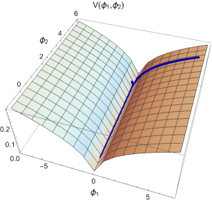
Figure 1: Two-field potential $V(\phi_{1},\phi_{2})$ for the model in eq. (1). Here $M_{1}=0.5M_{\mathrm{Pl}}$, $M_{2}/M_{1}=0.1$, $p_{1}=2/5$, $p_{2}=1$, $\mu_{1}=\mu_{2}=0.5$. The blue curve depicts a typical two-stage inflationary trajectory, where the field $\phi_{1}$ slides down the slope first, oscillates while decaying near the bottom of the “gutter”, and then $\phi_{2}$ starts to move along the “gutter”.

We have chosen to decouple the two axion sectors from each other for simplicity, and as a result the early inflationary trajectory and the late inflationary dynamics become two separate stages. Thus in this limit we can study the dynamics of inflation as a sequence of two consecutive single-field stages. As noted above, this could happen as a leading approximation in the case when the two sectors mix only gravitationally. As in [1] we view this as an interrupted N-flation [46], with a larger mass gap between the two inflatons, where one dominates early on, and drops out of slow roll well before the other one. Each effective action ${\cal L}_{i}$ is precisely the action of the k-inflation model of [50, 51], with a single dimensional normalizing scale, and the dimensionless coefficients of ${\cal O}(1)$ up to combinatorial factors set by normalizing Feynman diagrams. At strong coupling, where the theory (3) is driven by observations, it is this action which should be deployed to compute inflationary background and observables [10]. In Fig. 1, we illustrate the inflationary trajectory on the potential (1). In the present case, the segments of the trajectory are also affected by the higher derivative operators (2) which we retained.

We also note that an even more extreme reduction of $r$ can occur if the potential ${\cal V}_{eff}$ at large $\phi$ plateaus. In a sense, the change of the potential from convex to concave as strong coupling regime sets in may be viewed as a beginning of such plateauing. In some cases where additional control tools are present, namely AdS/CFT, and the corrections are enhanced by the presence of many flavors, such potentials could be constructed [9, 52]. In the example [9], the resulting effective potential is ${\cal V}_{eff}\sim(1-\frac{1}{1+(4\pi cm\varphi/M^{2})^{p}})$. In this case the tensor to scalar ratio is very small, $r\sim{\rm few}\times 10^{-4}$ [9, 10]. We will, however, not explore the detailed dynamics of such models here.

The next step is to recalculate the spectrum of perturbations on large scales. As before we solve the equations of motion for the inflaton and calculate the scalar spectral index $n_{s}$ and the tensor-to-scalar ratio $r$ at $N_{e}$ efolds before the end of the first stage, but now we include the effect of the higher derivative operators. This forces us to resort to numerical integration, and we will only present the result for the first stage of inflation since this is when the fluctuations distorting the CMB are generated. At this stage we can approximate the dominant contribution to the effective potential during the first stage by

$$V_{eff}(\phi_{1})=M_{1}^{4}\left[\left(1+\frac{\phi_{1}^{2}}{\mu_{1}^{2}}\right)^{\frac{p_{1}}{2}}-1\right]\simeq M_{1}^{4}\left[\left(\frac{\phi_{1}}{\mu_{1}}\right)^{p_{1}}-1\right]\,.$$ (4)

which in the plot of Fig. 1 corresponds to fixing $\phi_{2}$ at some value and rolling down the hill towards the ridge at a $\phi_{2}\simeq{\rm const.}$, thanks to $\phi_{2}\gg\mu_{2}$. Here, clearly, $M_{1}\simeq M/\sqrt{4\pi}$.

In the absence of higher derivative operators in [1] we could then use the slow roll parameters $\epsilon_{V}=\partial_{\phi}V_{eff}(\phi_{1})^{2}/(2V_{eff}(\phi_{1})^{2})$ to both control the numerical integration of the dynamics based on (4) in slow roll regime, and to compute the observables $n_{s}-1=2\eta_{V}-6\epsilon_{V}$, $r=16\epsilon_{V}$ at a value of $\phi_{1}$ when the first stage of inflation ends, which gives

$$N_{e}=\int_{\phi_{1}}^{\phi_{1}(end)}d\phi\,\frac{H}{\dot{\phi}}\simeq\left(\frac{\phi_{1}^{2}}{2p_{1}M_{Pl}^{2}}\right)\left[1-\frac{2}{2-p_{1}}\left(\frac{\mu_{1}}{\phi_{1}}\right)^{p_{1}}\right]\,$$ (5)

efolds before the end of the first inflationary stage. That generated the primordial tensor modes with $r$ in the range $0.02~{}\mbox{\raisebox{-2.58334pt}{$\stackrel{{\scriptstyle<}}{{\sim}}$}}~{}r~{}\mbox{\raisebox{-2.58334pt}{$\stackrel{{\scriptstyle<}}{{\sim}}$}}~{}0.06$ [1].

As noted [53, 10], higher derivative operators help reduce $r$ further. In this regime it is convenient to compute the cosmological observables using the k-inflation approach of [51, 54, 55]. Importantly, the speed of sound of the scalar perturbations $c_{s}$ is different from unity, so that the tensor-scalar ratio is $r=16c_{s}\epsilon$, and $\epsilon$ is the usual slow-roll parameter. In this case the inflationary consistency relation is $r=-8c_{s}n_{T}$, where $n_{T}$ is the tensor spectral index. What happens is that the higher derivatives improve the slow roll in the scalar field equation, without affecting the gravitational field equations. As a result, the noted modification of the consistency condition follows. Furthermore, the nonlinear terms in the fluctuations [54, 55] may yield non-negligible equilateral non-Gaussianities. We will also compute those numerically to show how the non-Gaussianities limit $r$ from below.

To do this, using the calculational framework of k-inflation, we restrict to the subcase when inflation is slow roll potential-driven, and require that higher derivative terms dominate over the quadratic ones both in controlling the background and the perturbations. For simplicity, we will present below only the equations for the truncation of the kinetic energy function to only quartic terms, $K={\cal Z}X_{1}+\tilde{\cal Z}\frac{16\pi^{2}X_{1}^{2}}{M^{4}}$. We will also consider the sextic derivative terms as an additional example, motivated by direct string theory constructions. Both of these ‘trans-quartic’ cases suppress $r$ more than the quartic truncations. But in weak coupling they can go only so far.

3 An Interlude with High Harmonics, for Strings

Before we proceed with computing the observables for the nonlinear theory we have set up so far, let us pause and consider in more detail the origin of the nonlinearities, and in particular the higher derivative terms. The higher derivative operators may arise in the weak coupling limit, in which case their coefficients may be calculable in perturbation theory. Generically this means the derivative-dependent part of the effective action will be truncated to a few leading terms (as noted in the perturbative analysis in [53], for example). The leading order terms are $\propto(\partial)^{4}$. However, although such terms can indeed arise already at weak coupling in string theory, their impact is limited. In this section we stipulate what one may expect in the controlled regime ‘under the lamppost’, below the strong coupling scale. Our aim is to outline a ‘perturbative’ boundary in the observable phase space, and to show by example how strong coupling effects can enhance the observable signals.

Which of the two ‘trans-quartic’ cases mentioned above depends on the nature of the underlying monodromy inflaton candidate. If the inflaton scalar arises as a position modulus of a mobile D-brane acquiring monodromy e.g. via moving along a non-trivial fibration of the compactification space, its kinetic term may pick up higher- derivative corrections to all orders from the DBI action of the moving D-brane generating the inflaton scalar potential as well. As a guiding example, we look e.g. at the D7-brane monodromy inflation model in [56] where the D7-brane position in the transverse extra dimensions is the inflaton candidate. F-theory there allows the authors to describe the D7-brane position as part of the elliptic Calabi-Yau 4-fold complex structure moduli. Therefore, the 7-brane position acquires its two-derivative kinetic term from a Kahler potential in the effective 4D supergravity.

However, at least in the perturbative type IIB string theory limit of F-theory, this two-derivative kinetic for the D7-brane position is ultimately obtained via matching the expansion of the full DBI action of the D7-brane effective action in [57] up to two-derivative order. Hence, in the type IIB limit we expect the full kinetic term of the D7-brane position scalar inflaton candidate for the model of [56] to take the complete DBI form. We leave a full discussion of these arguments for future work, but note that they provide plausibility for the appearance of the full infinite higher-derivative kinetic term series of DBI inflation in brane monodromy inflation setups of schematic type $\sqrt{1-\alpha^{\prime}\dot{x}_{\bot}^{2}}$ such as seen e.g. in [39], as they rely just on the structure of the DBI action as the universal part of the perturbative effective description of D-branes.

In contrast, if inflation arises as axion monodromy from a bulk $p$-form string axion, this will not acquire contributions to its kinetic term from branes and thus no DBI-type kinetic term. Instead, the supersymmetric completion of the leading higher-order $\alpha^{\prime 3}R^{4}$ [58] curvature correction is expected to generate corrections to the kinetic term of bulk closed string axions up to sextic order from terms containing at least one power of curvature. This expectation arises from considering the SUSY completion of the type II $\alpha^{\prime 3}R^{4}$ correction. While this completion in its full form is unknown as of today, the bosonic sector of the completion, as sketched in e.g. [59], is expected to contain terms reading schematically as

$$\Delta{\cal L}_{\alpha^{\prime 3}R^{4}}^{SUSY,bos.}\supset{R^{3}F_{p}^{2},R^{3}|F_{p}|^{2},R^{2}F_{p}^{4},R^{2}|F_{p}|^{4},RF_{p}^{6},R|F_{p}|^{6}}\quad.$$ (6)

The non-vanishing invariant tensor contractions among them clearly generate axion kinetic term corrections up to sextic order arising from the powers of $|F_{p}|^{2}$. Moreover, the possible invariants generating these higher-order axion kinetic terms may involve topological invariants of the compactification space arising from integrating over powers of curvature on the internal space. These topological invariants, like e.g. the Euler characteristic, may lead to sizable numerical enhancements of the higher-order axion kinetic terms, providing a rationale for their mass scales to scan a range of values relative to the Planck scale.

The higher-derivative axion kinetic term series inferred from the SUSY completion of the $\alpha^{\prime 3}R^{4}$ terminates at a finite order of derivatives at this order in $\alpha^{\prime}$. String theory is expected to generate corrections beyond ${\cal O}(\alpha^{\prime 3})$ in an infinite series. This is of course a string theory avatar of our strong coupling EFT argument. Hence, at higher orders in $\alpha^{\prime}$ there will potentially exist invariants involving powers of the $p$-form field strengths producing higher-derivative axion kinetic terms beyond the maximal order generated at ${\cal O}(\alpha^{\prime 3})$. But in weak coupling these terms will be small. The closed string sector higher-order $\alpha^{\prime}$-corrections appear after reduction to 4D suppressed by powers of the inverse compactification volume [59].

Hence, barring an appearance of numerically very large topological numbers governing these higher-order $\alpha^{\prime}$-corrections, the higher-derivative axion kinetic terms potentially produced by them will have volume suppressed small coefficients relative to the higher-derivative axion kinetic terms appearing at ${\cal O}(\alpha^{\prime 3})$. In this sense the series of higher-derivative axion kinetic terms with potentially sizable coefficients appearing via dimensional reduction from the 10D closed string sector will effectively terminate at sextic order. In other words, to get larger effects one must approach the limits of the validity of the compactified theory, as expected from the generic EFT consideration.

Again, we stress that the above observations about (ir)relevance of higher derivative terms are features of the weak coupling limit of the theory, well below the relevant cutoff of the inflationary EFT, and under the assumption that the Hilbert space of states is largely unaffected by the background evolution of fields and couplings. As we approach the limits of the inflationary EFT, by cranking up the field values and couplings, the irrelevant operators, including the higher derivative ones, will become more influential. To account for those effects, we must be careful when comparing the higher-derivative axion kinetic terms arising from dimensional reduction of the 10D higher-derivative $p$-form field strength powers to the higher-derivative axion kinetic terms outlined in [10]. It is here where the origin of the low energy axions is important. The point is that simple ‘derivative accounting’ may be misleading, which can be seen as follows. Consider a low energy EFT axion, which acquires its quadratic potential via mixing with the 4-form field strength in the 4D effective flux monodromy description of [41], and is a pseudo-scalar magnetic dual of a perturbative $p$-form string axion, that comes from dimensional reduction. At two-derivative level all the known string axion and brane monodromy inflation mechanisms can be dualized into this 4D effective 4-form description [60]. This procedure is useful since it makes the hidden gauge symmetries of the theory manifest, providing the tools to control the strong coupling regime. However, it also shows that once the dimensionally reduced $p$-form string axions acquire higher-derivative kinetic terms, it becomes quite non-trivial to match these to the description of the higher-derivative kinetic terms of the dual axion of the 4D effective 4-form theory, as encoded in couplings of the type $(A_{3}-dB_{2})\wedge\star F_{4}$ with $B_{2}$ being the 4D dual 2-form gauge potential describing the axion degree of freedom from the compactified string model. In a nutshell, dualization is a canonical transformation [61, 43], and so in perturbation theory, the derivatives of the axion are mapped to the powers of the 3-form mass term and vice versa. This is simply the consequence of the fact that a canonical transformation exchanges generalized coordinates and momenta, $(q,p)\leftrightarrow(-P,Q)$, while preserving the commutation relations and the Hamiltonian [61, 43]. The full “resummation” of the perturbative duality maps also “dresses” up the Hilbert space vacuum, very similarly to what happens with the BCS vacuum below the critical temperature, when the condensate forms. Thus it is perfectly plausible that a theory with higher derivatives on one side may appear as a totally non-derivative theory on the other side.

A flavor of the non-trivial duality matching is already visible in the 4-form description of hybrid axion monodromy in [62], where the nontrivial issues concerning the selection of the vacuum are noted. Here, we set such a full duality matching at higher-derivative order aside given the uncertainties with the perturbative dimensionally reduced $p$-form string axion sector at higher derivatives. We do expect that upon performing the duality match the finite order of the higher-derivative axion kinetic terms expected for a closed string axion at ${\cal O}(\alpha^{\prime 3})$ will translate to a matching finite higher-derivative order of the kinetic terms for the dual 4D effective axion of the 4-form EFT, which suffices for our purposes. We should also note that even when the strong coupling effects induce large higher derivative operators, there are still regimes where initial conditions for classical evolution allow flattened potentials to dominate, thus ‘deactivating’ the higher derivative terms [10]. This regime is also illustrated by our truncation of the derivative expansion. Obviously, this means there could be other branches of solutions which we ignore here.

4 Variations for BICEP3

Having set up the stage for the EFT of double monodromy, with or without strong coupling effects included, and highlighted its relationship to the UV completions in models where inflatons are axions or brane positions, we can now leverage the universality of the 4D EFT to study the axion inflation dynamics at strong coupling. The homogeneous field configurations satisfy $16\pi^{2}X_{1}/M^{4}\gtrsim 1$ and $16\pi^{2}V_{eff}/M^{4}\gtrsim 1$. Truncating to the quartic time derivative terms for simplicity, as outlined above, the slow roll field equations are 

$$3M_{\mathrm{Pl}}^{2}H^{2}=V_{eff}\,,~{}~{}~{}~{}~{}~{}~{}~{}~{}~{}~{}~{}~{}6H\dot{\phi}_{1}\tilde{\cal Z}X_{1}=-4\pi M^{2}mV_{eff}^{\prime}\,.$$ (7)

There are evolutionary regimes for the fields depending on the relevance of the derivative terms relative to the potential. A discussion of options was given in [10]. A case of interest to us here is where the higher derivative operators are both large in the EFT, and are excited, contributing to the background during slow-roll inflation. In this case the tensor power is suppressed thanks to both the flattened potential and the subluminal speed of sound of the perturbations, induced by the higher derivatives. An important additional consideration is that the higher derivative terms induce nonlinearities which yield non-Gaussianities. The bounds on non-Gaussianities, $f_{NL}~{}\mbox{\raisebox{-2.58334pt}{$\stackrel{{\scriptstyle<}}{{\sim}}$}}~{}{\cal O}(10)$ imply a lower bound on $r$.

To compute the perturbations on the background controlled by the slow roll equations (7), we deploy the formalism of the inflaton EFT [63], ignoring the mixing with gravity. This approximation is good at energy scales $E\gg\sqrt{\epsilon}H$ and $c_{s}^{2}\gg\epsilon$, which apply in our case. The spectrum of perturbations is almost scale-invariant and has small non-Gaussianities, as observations require. In the gauge where the spatial metric is unperturbed, the field perturbation is $\phi_{1}(t,\vec{x})=\varphi_{0}(t+\pi(t,\vec{x}))$ whereas the spatial curvature perturbation is ${\cal R}=-H\pi$. Expanding Eq. (3) up to third order, and keeping only the terms lowest in derivatives,

$$S=-\int dtd^{3}\vec{x}\,a^{3}M_{\mathrm{Pl}}^{2}\dot{H}\left[\frac{1}{c_{s}^{2}}\dot{\pi}^{2}-\frac{(\partial_{i}\pi)^{2}}{a^{2}}+\left(\frac{1}{c_{s}^{2}}-1\right)\left(\dot{\pi}^{3}+\frac{2}{3}c_{3}\dot{\pi}^{3}-\dot{\pi}\frac{(\partial_{i}\pi)^{2}}{a^{2}}\right)\right]\,.$$ (8)

Dropping the subscript $"1"$ from here on, and using our monodromy EFT (3), the speed of sound is $c_{s}^{2}=\partial_{X}{\cal K}/(\partial_{X}{\cal K}+2X\partial_{X}^{2}{\cal K})$, and $c_{3}(1/c_{s}^{2}-1)=2X^{2}\partial_{X}^{3}{\cal K}/\partial_{X}{\cal K}$. So when $X>\frac{M^{4}}{16\pi^{2}}$, we find $c_{s}^{2}\sim\frac{M^{4}}{32\pi^{2}X}\frac{{\cal K}^{\prime\prime}}{{\cal K}^{\prime}}$ and $c_{3}(1/c_{s}^{2}-1)=\frac{512\pi^{4}X^{2}}{M^{8}}\frac{{\cal K}^{\prime\prime\prime}}{{\cal K}^{\prime}}$, or $c_{3}=\frac{16\pi^{2}X}{M^{4}}\frac{{\cal K}^{\prime\prime\prime}}{{\cal K}^{\prime\prime}}$. The exact details of the theory when $y=16\pi^{2}X/M^{4}>1$, which set the magnitude of ${\cal K}$ and its derivatives, depend on the UV theory governing the large-$y$ asymptotia.

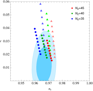
Figure 2: Tensor-to-scalar ratio versus spectral index for double monodromy with quartic (left) and sextic (right) kinetic terms, compared to the data of [4]. In the left panel, $K(X)=X+X^{2}/M_{4}^{4}$, with $M_{4}=0.05$, while in the right panel, $K(X)=X+X^{3}/M_{6}^{8}$, fixing $M_{6}=0.05$. We take $\mu_{1}=0.01$, and vary $0.1\leq p_{1}\leq 0.5$. The triangles depict the quadratic kinetic term case $(c_{s}=1)$, while dots are the predictions for the higher derivatives. A finite $M_{4}$ or $M_{6}$ will give a redder spectrum [64], and a lower $r$.

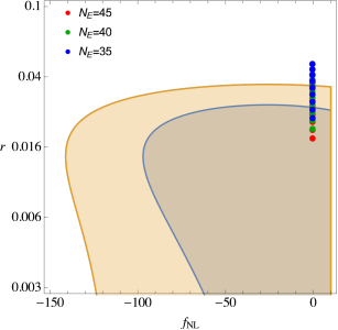
Figure 3: Tensor-to-scalar ratio $r$ v.s. equilateral non-Gaussianity $f_{\mathrm{NL}}$ for double monodromy with quartic (left) and sextic (right) kinetic terms. The parameters are the same as in Fig. 2. Because of the lower bound on $c_{s}$ in either model ($c_{s}^{2}>1/3$ for quartic, $c_{s}^{2}>1/5$ for sextic), the non-Gaussianity is very small.

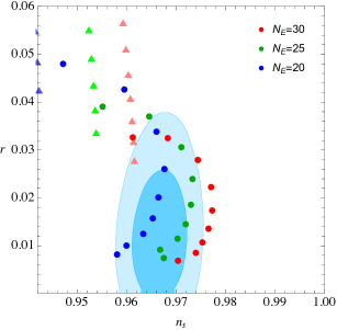
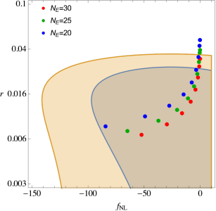
Figure 4: Tensor-to-scalar ratio $r$ versus spectral index $n_{s}$ (left) and $r$ versus equilateral non-Gaussianity $f_{\mathrm{NL}}$ (right) for double monodromy with DBI kinetic terms. We take $\mu_{1}=0.01$ for the potential, vary $0.1\leq p\leq 0.5$ and fix $M=0.23$. In the left panel, the triangles denote solutions with the canonical kinetic term, while the dots are solutions for the DBI kinetic term. We note that, since $c_{s}$ is not bounded from below, $r$ can be much lower in the DBI model with respect to quartic and sextic kinetic terms. Equilateral non-Gaussianity shows the expected inverse correlation with $r$, but it is within the current experimental bounds.

As in weak coupling, the amplitude perturbation is controlled by horizon scale when $\lambda^{-1}\simeq H$. The Gaussian curvature perturbation is determined by folding this scale with the time translation breaking scale. In contrast to the weak coupling regime, where $\sqrt{\dot{\varphi}}=(2M_{\mathrm{Pl}}^{2}\dot{H})^{1/4}=\epsilon_{H}^{1/4}\sqrt{2M_{\mathrm{Pl}}H}\gg H$, in the strong coupling regime with large derivative terms one finds that this scale is $f_{\pi}^{4}=2M_{\mathrm{Pl}}^{2}\dot{H}c_{s}$. Note, that by Eq. (3) in this regime $M_{\mathrm{Pl}}^{2}H^{2}\simeq\frac{M^{4}}{16\pi^{2}}$. The Gaussian scalar power spectrum is $\Delta_{\mathcal{R}}^{2}\propto(H/f_{\pi})^{2}$.

The leading non-Gaussianities in this regime come from the 3-point function. There are two operators in (8) which source them. However since by naturalness and naïve dimensional analysis arguments all the derivatives are comparable, $c_{3}\simeq c_{s}^{2}<1$, and so the non-Gaussianities generated by $\sim c_{3}$ term are subleading. Thus the amplitude of the cubic non-Gaussianities reduces to a single narrow strip [10]. Using the perturbation potential

$$\langle\Phi_{\vec{k}_{1}}\Phi_{\vec{k}_{2}}\Phi_{\vec{k}_{3}}\rangle=(2\pi)^{3}\delta_{D}(\vec{k}_{1}+\vec{k}_{2}+\vec{k}_{3})\frac{6\Delta_{\Phi}^{2}}{(k_{1}+k_{2}+k_{3})^{3}}\left[f_{\rm NL}^{(1)}F_{1}(k_{1},k_{2},k_{3})+f_{\rm NL}^{(2)}F_{2}(k_{1},k_{2},k_{3})\right]\,,$$ (9)

we find that the $F_{1}$ and $F_{2}$ are induced by the $\dot{\pi}(\partial\pi)^{2}$ and $\dot{\pi}^{3}$ operators, respectively [55, 65, 66]. Explicitly, we define

$$K_{1}=k_{1}+k_{2}+k_{3}\,,\quad K_{2}=(k_{1}k_{2}+k_{2}k_{3}+k_{3}k_{1})^{1/2}\,,\quad K_{3}=(k_{1}k_{2}k_{3})^{1/3}\,,$$ (10)

in terms of which

$$F_{1}=-\frac{9}{17}\frac{12K_{3}^{6}-4K_{1}K_{2}^{2}K_{3}^{3}-4K_{1}^{4}K_{2}^{2}+11K_{1}^{3}K_{3}^{3}-3K_{1}^{4}K_{2}^{2}+K_{1}^{6}}{K_{3}^{9}}\,,$$

$$~{}~{}~{}~{}~{}~{}~{}~{}~{}~{}~{}~{}~{}~{}~{}~{}~{}~{}~{}~{}~{}~{}~{}~{}~{}~{}~{}~{}~{}~{}F_{2}=\frac{27}{k_{1}k_{2}k_{3}}\,.$$ (11)

The term $\propto F_{1}$ describes equilateral non-Gaussianities, since the momentum dependence is such that it is maximized when all three momenta are equal, while the term $\propto F_{2}$ shows an important contribution also on flattened triangles. CMB analyses [65, 66] are commonly done in terms of two templates, the equilateral one which is very similar to $F_{1}$, and an orthogonal one which is a linear combination of $F_{1}$ and $F_{2}$. In terms of the Lagrangian parameters, the $f_{NL}$ coefficients are

$$f_{NL}^{(1)}=-\frac{85}{324}\left(\frac{1}{c_{s}^{2}}-1\right)\,,\qquad f_{NL}^{(2)}=-\frac{10}{243}\left(1-c_{s}^{2}\right)\left(\frac{3}{2}+c_{3}\right)\,.$$ (12)

For our quartic and sextic models, $c_{3}$ in eq. (12) is $-3$ and $-4$, respectively, so $f_{\rm NL}^{(2)}$ is very small with respect to $f_{\rm NL}^{(1)}$, by a factor $c_{s}^{2}$; for DBI, $f_{\rm NL}^{(1)}=-(17/4)f_{\rm NL}^{(2)}$, and they have the same dependence on $c_{s}^{2}$. For definiteness, we show $f_{\rm NL}^{(1)}$ in Figs. 3 and 4. The experiments are already constraining the phase space of even the strongly coupled theory. From Planck [67], marginalizing over $c_{3}$, one gets the bound $c_{s}~{}\mbox{\raisebox{-2.58334pt}{$\stackrel{{\scriptstyle>}}{{\sim}}$}}~{}0.21$. This yields $X~{}\mbox{\raisebox{-2.58334pt}{$\stackrel{{\scriptstyle<}}{{\sim}}$}}~{}M^{4}/10$. Thus the theory should be in strong coupling to prevent too large $r$, but it cannot be arbitrarily strongly coupled to satisfy the bound on non-Gaussianities. Hence the tensor power cannot be arbitrarily weak.

In Fig. 2 and 3 we show the predictions for the observables $r$, $n_{s}$ and $f_{\mathrm{NL}}$, for our potential Eq. (4) and kinetic terms with either quartic or sextic higher derivative terms, in a regime in which these higher derivative corrections are important. In Fig. 4, we show the predictions for our double mondromy potential with a DBI kinetic term, $K(X)=M^{4}\left(1-\sqrt{1-2X/M^{4}}\right)$ which produces an infinite series of higher derivative corrections. In comparing to the results of [64] it is important to note that there the higher derivatives arise from integrating out a heavy scalar generating an infinite series of higher derivative operators. In the particular example displayed in Fig. 5 in [64], this infinite series re-sums into a cosine potential in $V$ and a cosine dependence in $c_{s}$. This produces the strong reddening of $n_{s}$ with decreasing $c_{s}$ visible in the blue down-left curving band of Fig. 5 of [64]. In our first example we only keep a quartic and/or sextic higher derivatives in the kinetic term, hence the reddening of $n_{s}$ remains much milder for our case. Moreover, with decreasing $c_{s}$ and thus increasing effects of the higher derivative operators, we get pushed out of the quadratic part of the scalar potential onto the flatter-monomial ‘wings’ which causes a blue-shift of $n_{s}$ partially offsetting the reddening effects of the higher derivatives themselves. Meanwhile, in the example of Fig. 5 in [64] decreasing $c_{s}$ and thus increasing effects of the higher derivatives pushes one towards the hill-top of a cosine potential which by itself causes additional reddening of $n_{s}$.

For the quartic and sextic kinetic terms, we observe that for powers $p~{}\mbox{\raisebox{-2.58334pt}{$\stackrel{{\scriptstyle>}}{{\sim}}$}}~{}0.1$, we get small non-Gaussianities, tensor to scalar ratio in the range $r~{}\mbox{\raisebox{-2.58334pt}{$\stackrel{{\scriptstyle>}}{{\sim}}$}}~{}0.015$, and $0.96~{}\mbox{\raisebox{-2.58334pt}{$\stackrel{{\scriptstyle<}}{{\sim}}$}}~{}n_{s}~{}\mbox{\raisebox{-2.58334pt}{$\stackrel{{\scriptstyle<}}{{\sim}}$}}~{}0.97$ for the first stage of inflation which ends after $35-45$ efolds. For the DBI kinetic term, we get $r~{}\mbox{\raisebox{-2.58334pt}{$\stackrel{{\scriptstyle>}}{{\sim}}$}}~{}0.006$ and larger $f_{\mathrm{NL}}$ for the first stage of inflation ending after $20-30$ efolds. Summarizing, with non-standard kinetic terms the model remains a fully viable fit of the sky at the CMB scales, but with predictions in the reach of the near future cosmological observations, such as the next installment of BICEP, or LiteBIRD. This makes our natural monodromy models an excellent benchmark for future observations. Further, the mechanism of nonperturbative generation of chiral tensors, using vector tachyon instability [68, 69, 1], which we review below in this new context, remains operational and can yield additional gravity wave signals at shorter scales.

5 Für LISA, an Encore, with Other Instruments Too

We noted in [1] that axion-like inflatons often couple to $U(1)$ gauge fields via the standard dimension-5 operators $\propto\phi_{1}F_{\mu\nu}\tilde{F}^{\mu\nu}/2$. A simple example is to start with a $4$-form field strength in $11D$ Sugra, with Chern-Simons self-couplings, and dimensionally reduce it on some toroidal compactification. Ignoring the moduli fields the resulting $4D$ effective action will include light axions coupled to dark $U(1)$s since

$$-F_{abcd}^{2}+\epsilon_{a_{1}\ldots a_{11}}A^{a_{1}\ldots}F^{a_{4}\ldots}F^{a_{8}\ldots a_{11}} \ni -F^{2}_{\mu\nu\lambda\sigma}-(\partial\phi_{1})^{2}-\mu\phi_{1}\epsilon_{\mu\nu\lambda\sigma}F^{\mu\nu\lambda\sigma}$$ (13)

$$-\sum_{k}F^{2}_{\mu\nu\,(k)}-\frac{\phi_{1}}{f_{\phi}}\sum_{k,l}\epsilon_{\mu\nu\lambda\sigma}F^{\mu\nu}{}_{(k)}F^{\lambda\sigma}{}_{(l)}\,.$$

Here the first line lists the $4$-form-axion sector, which thanks to the monodromy coupling is massive but light, and the second describes the mixing of the axion with dark $U(1)$s. If for simplicity we take only one coupling to be nonzero, we can model it with the canonically normalized $4D$ dimension-5 operator

$$\mathcal{L}_{\rm int}=-\sqrt{-g}\frac{\phi_{1}}{4f_{\phi}}F_{\mu\nu}\tilde{F}^{\mu\nu}\,,$$ (14)

where $f_{\phi}$ is sub-Planckian. This scale is generically $\simeq M_{GUT}$ (see e.g. [47, 48]). A rolling axion triggers the tachyonic instability of one circular polarization of the gauge field [70], whose exponential production both backreacts on the inflaton and produces scalar and tensor perturbations [68, 69]. Details of the backreaction were examined in [71, 72], and a very comprehensive analysis of these effects was provided recently in [73], with the results of the non-perturbative treatment recently cross-verified in [74] using a completely different gradient expansion formalism down to numerically identical predictions of the GW signal including resonance-induced peaked fine structure. The details of the dynamics are given in [73, 1] and we will not repeat them here. We should mention the other works which have recently explored bumpy early universe dynamics to generate relic gravity waves [75, 76, 77, 78, 79, 80, 81].

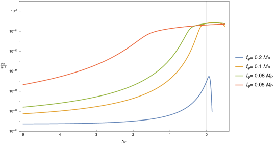
Figure 5: Evolution at the end of the first inflationary stage of the energy density in gauge fields. We denote by $N_{e}$ the number of efolds before the end of the first stage of inflation, and we normalize the energy density to $M_{\mathrm{Pl}}^{4}$. The parameters of the potential are fixed for convenience to $M_{1}^{4}=2\times 10^{-9}M_{\mathrm{Pl}}^{4}$, $\mu_{1}=M_{\mathrm{Pl}}$, $p=0.2$; at the CMB scales they lead to similar results as $\mu_{1}=0.1M_{\mathrm{Pl}}$, which fit CMB perfectly. We show results for different couplings $f_{\phi}$ as shown in the legend. The vertical line denotes the end of inflation, and the solutions we show are not completely reliable there. Note that the contributions of the vector field are very small until the very end of inflation, when $\phi_{1}$ moves the fastest. As a result the U(1) production does not affect CMB significantly.

We imagine this axion to be the inflaton dominating the first stage of inflation in the double monodromy inflation of the previous section, which in addition to the simple quadratic potential (given in the dual $4$-form frame by the first line of Eq. (13)), also includes additional corrections, that combine into the potential (1) and the higher derivative operators (2). Thus early on during the first stage of inflation, the dynamics described in the previous section yields a suppressed tensor-to-scalar ratio and weak non-Gaussianities, while matching the scalar CMB spectrum. By the end of this stage, however, the inflaton drops out of the strong coupling, and inflation continues for a few more efolds in weak coupling. This last epoch of the first stage of inflation is described by the terms of Eq. (13). Hence the analysis of sub-CMB gravity wave generation of [1], describing how the tachyonic instability in the dark $U(1)$ is triggered by (14) goes through unabated. Hence, a $U(1)$ chirality is cranked up and it in turn sources chiral gravity waves. The amplification is quite efficient, although it is bounded by inflaton kinetic energy and scale of the first stage of inflation near its end. Assuming that the potential (4) remains valid all the way to the end of the weakly coupled epoch of the first stage of inflation, the energy density transferred to the tachyonic chirality of the dark $U(1)$ can be calculated numerically, as presented in Fig. 5.

We should stress that some of these modes will reenter the horizon during the intermediate matter-dominated stage, interrupting the two stages of inflation. Hence they would dilute by expansion during that epoch. However as long as the interruption is short the dilution is weak. We can estimate it as follows: for subhorizon wavelength modes, the amplitude goes as $1/\lambda\sim 1/a$, where $a$ is the scale factor. Since these modes are harmonic oscillators, their power, by virial theorem, is given by the square of frequency $\times$ the amplitude. Hence the suppression factor will be at most $(a_{1}/a_{2})^{4}$ where $a_{1}$ is the scale factor at the end of stage 1 of inflation, and $a_{2}$ the scale factor at the mode re-freezing after the start of the next stage inflation. This factor is largest for the shortest wavelength mode at the end of stage 1, for which $k/a_{1}\sim H_{1}$. Because the mode freeze-out yields $k/a_{2}\simeq H_{2}$, this yields $a_{1}/a_{2}~{}\mbox{\raisebox{-2.58334pt}{$\stackrel{{\scriptstyle<}}{{\sim}}$}}~{}H_{2}/H_{1}$, and so for a short interruption the power suppression would be no more than a factor of 100 to 1000, which is why we ignored it here. A more precise calculation is warranted here, both for the computation of the proper signal benchmarks and, crucially, since this also evades violations of the BBN bound on gravity waves, $\Omega_{GW}h^{2}\lesssim 10^{-6}$ [82]. For this reason, we sketch these uncertainties in the prediction, plotting a gray band, spanning two orders of magnitude, around the idealized prediction of the power emitted in GWs in Fig. 6, 7 below.

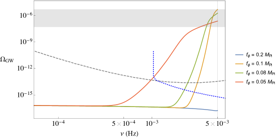
Figure 6: Abundance of gravitational waves as a function of frequency, setting $N_{\rm CMB}=35$. The dashed grey line is the sensitivity of LISA [83] and the dotted blue line is the sensitivity of Big Bang Observer (BBO) [84]. Again, we use $M_{1}^{4}=2\times 10^{-9}M_{\mathrm{Pl}}$, $\mu_{1}=M_{\mathrm{Pl}}$, $p=0.2$ for convenience, and as before scan $f_{\phi}$ as shown in the legend. The vertical line again designates the end of inflation, beyond which a different approximation is needed. We plot maximal power here ignoring the suppression during the interruption. The gray band outlines the uncertainties due to this suppression, which when accounted for evade violations of the BBN bound on gravity waves.

In turn the tachyonic dark $U(1)$ modes source the stochastic gravity waves which are chiral, with the total abundance which can be estimated by [85]

$$\Omega_{GW}\equiv\frac{\Omega_{r,0}}{24}\Delta_{T}^{2}\simeq\frac{\Omega_{r,0}}{12}\left(\frac{H}{\pi M_{\mathrm{Pl}}}\right)^{2}\left(1+4.3\cdot 10^{-7}\frac{H^{2}}{M_{\mathrm{Pl}}^{2}\xi^{6}}e^{4\pi\xi}\right)\,,$$ (15)

where $\Omega_{r,0}=8.6\cdot 10^{-5}$ is the radiation abundance today, $\xi=\frac{\dot{\phi}}{2Hf_{\phi}}$ and the terms are evaluated at horizon crossing. The equation is valid for $\xi\gtrsim 3$. This is the sum of the two polarization of gravitational waves: the $"1"$ term in the parenthesis arises due to the usual metric fluctuations in de Sitter space, and includes the contributions from both graviton helicities. The second term in parenthesis, involving the exponential amplification, receives contribution only from the helicity sourced by the ‘tachyonic’ gauge field source, as evidenced by its dependence on $\xi$. By mode orthogonality in the linearized limit, the other graviton helicity is not enhanced.

It is clear that a favorable realization of the scales can enhance the primordial GW spectrum dramatically. To fix the physical wavelength of these modes, which allows us to see by which instrument they might be searched for, and what their amplitude at the relevant wavelength is, we can rewrite $\Omega_{GW}$ as a function of the frequency observed at the present time. Since the comoving frequency is $\nu=k/(2\pi)$, the frequency of the modes in terms of the number of efolds before the end of inflation is given by

$$N=N_{CMB}+\ln\frac{k_{\rm CMB}}{0.002\textrm{Mpc}^{-1}}-44.9-\ln\frac{\nu}{10^{2}\textrm{Hz}}\,,$$ (16)

where $k_{CMB}=0.002\textrm{Mpc}^{-1}$ is the CMB pivot scale, and $N_{\rm CMB}$ is the number of efolds before the end of the first stage of inflation where the CMB scales froze out. With this we can regraph the results of Fig. 5 in terms of the new independent variable $\nu$ and the GW amplitude $\Omega_{GW}$. The results are presented in Fig. 6. Again the approximations which we employ are not completely reliable beyond the end of inflation, and noted above and in [1]. However they remain a good indicator of the signal’s power.

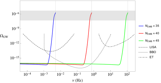
Figure 7: Abundance of gravitational waves as a function of frequency, setting for different $N_{\rm CMB}=35,40,45$. We show the predicted bounds as a function of frequency for LISA [83], Big Bang Observer (BBO) [84] and Einstein Telescope (ET) [86]. We use $M_{1}^{4}=2\times 10^{-9}M_{\mathrm{Pl}}$, $\mu_{1}=M_{\mathrm{Pl}}$, $p=0.2$, $f_{\phi}=0.08$. If $n_{s}$ is bluer, for monodromy models this means longer (first stage of) inflation. If at the end of this stage chiral tensors are generated, their frequency will be higher. The vertical line designates the end of inflation for each curve, beyond which a different approximation is needed. Again the gray band outlines the uncertainties in the prediction of the power due to the suppression at the interruption between the stages of rollercoaster inflation.

Of course, as we have seen from the previous discussion, and showed manifestly in e.g. Fig. 2, we can automatically satisfy the CMB bounds on $n_{s}$ and $r$ for a range of $N_{CMB}$. This means, that there are degeneracies in the evolution allowing for a good fit the CMB for a range of models, with different values of the pivot point $N_{CMB}$ – i.e. with the “CMB epoch” of multistage inflation of varying duration. Therefore we find it interesting to fix $f_{\phi}$ and plot $\Omega_{GW}(\nu)$ for different values of $N_{CMB}$, which generates a horizontal shift of the curves of Fig. 6. This plot is in Fig. 7, from which it is apparent that several experiments in the near future can explore the parameter space of our model. What’s more is that such a mechanism might occur at the end of every accelerated stage of rollercoaster, due to the inflatons being axion-like and possibly coupling to many different dark $U(1)$s, thus producing what we might dub a “characteristic spectrum” of rollercoaster models. If so then each spike, a different range of scales, might be simultaneously probed by one of the planned instruments.

The bottomline is that these modes may very well be out there for the GW instruments to discover. Depending on the specifics of the earliest stage of inflation and its duration, their wavelength might be in the sweet spot of LISA [83] or DECIGO/BBO [84], or if the wavelength is longer (and the earlier stage of inflation shorter), SKA or NANOgrav (for a recent study of the measurement of the spectrum of primordial gravitational waves see [87]). In either case, combining this with the bounds on $r$ at the CMB scales makes our double-coaster, and more generally multistage rollercoaster, extremely predictive and easy to confirm.

6 Outro

We have updated here our earlier model of double monodromy inflation with the inclusion of the general strong coupling-induced irrelevant operators, which lead to additional suppression of the tensor to scalar ratio in inflation. As a result, the predictions of the model, which involves an early stage of inflation which is interrupted by the first inflaton decay $25-40$ efolds after the beginning, are fully consistent with the most recent BICEP/Keck bounds. The observables are $0.006~{}\mbox{\raisebox{-2.58334pt}{$\stackrel{{\scriptstyle<}}{{\sim}}$}}~{}r~{}\mbox{\raisebox{-2.58334pt}{$\stackrel{{\scriptstyle<}}{{\sim}}$}}~{}0.035$ with $0.96~{}\mbox{\raisebox{-2.58334pt}{$\stackrel{{\scriptstyle<}}{{\sim}}$}}~{}n_{s}~{}\mbox{\raisebox{-2.58334pt}{$\stackrel{{\scriptstyle<}}{{\sim}}$}}~{}0.97$ with $f_{NL}~{}\mbox{\raisebox{-2.58334pt}{$\stackrel{{\scriptstyle<}}{{\sim}}$}}~{}{\cal O}(10)$. This makes the models very predictive since they can be constrained – and possibly confirmed and ruled out – by the very near future observations. In addition the first inflaton could couple to a hidden sector $U(1)$ and lead to an enhanced production of vectors near the end of the first stage of inflation. These vectors in turn would source tensors at shorter wavelengths, leading to additional signatures of the model that would correlate with the signatures in the CMB.

In closing we should finally mention that at this point however it may still be premature to take the $n_{s}-r$ bounds as very strong obstructions to inflationary models. Namely, although the bounds on $r$ are strong, the correlation of $n_{s}$ and $r$ might be weaker than it seems. We believe the situation warrants a warning of sorts since the $n_{s}-r$ correlation is commonly used to assess the likelihood of popular inflationary models (nice reviews of the observational constraints on theoretical models can be found in, e.g. [2, 3]). For example, one commonly encounters the “potato plots” such as Fig. (5) in reference [4], or Fig. 4 in the subsequent paper [88], as well as our own Fig. 2 - 4, which one may take to suggest there is very small remaining parameter space for inflationary models to ‘squeeze in’. Such reasoning might be too quick, since there is another interesting possibility that can open up the space in the $n_{s}-r$ plane, which is quite curious although it might seem somewhat extreme.

The issue is that in all the figures plotting $r$ versus $n_{s}$ which we have shown so far, we have relied on the constraints on $n_{s}$ based on the CMB data analysis assuming the $\Lambda$CDM model of the late universe. However, for some years now, the measurements of the Hubble parameter using standard candles [15, 16, 19, 24] have shown discrepancy with the value of $H_{0}$ determined by Planck experiment, which is based on fitting the CMB data to the late $\Lambda$CDM cosmology [89]. To resolve the Hubble tension, many models have been proposed to date (for reviews see [22, 23]). Among the most successful models are the so called “Early Dark Energy” proposals, which involve additional degrees of freedom before recombination [90, 91, 20, 21]. Analyzing the CMB data in terms of these new models, a common feature is that the spectral index is bluer with respect to the $\Lambda$CDM value (see [17, 92, 93, 94, 95]). If it indeed turns out that the Hubble tension is real, and the most recent examinations indicate support for this option, assessing the discrepancy to be at $5\sigma$ at this time [24], the shift of $n_{s}$ will have very important implications for inflationary model constraints.

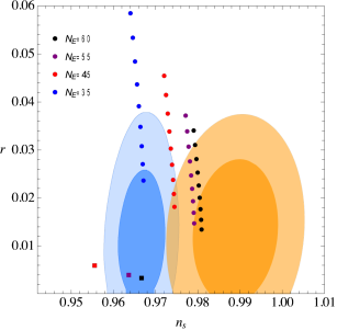
Figure 8: Tensor-to-scalar ratio $r$ versus spectral index $n_{s}$, for the $\Lambda$CDM model (blue) and for the NEDE model (gold). To get the NEDE model constraint, we approximate the $\Lambda$CDM contour as a bivariate Gaussian, and substitute the mean and error on $n_{s}$ by the ones got in the NEDE model. This approximate procedure reproduces well a full analysis [93]. The round dots are predictions of potentials (1) with $0.1\leq p_{1}\leq 0.5$, as before. The square dots are the predictions of the Starobinsky $R^{2}$ inflation [96].

We illustrate this in Fig. 8, where we plot the contours obtained from the $\Lambda$CDM model, and the one we infer from the constraints on $n_{s}$ in the so-called NEDE model, presented in [20, 21]. This plot clearly shows how – all of a sudden – flattened monodromy models, with a long stage of inflation, and the power law behavior of, for example, $\sim\phi^{1/2}$ at large $\phi$, which were supposedly excluded by having too large an $n_{s}$, may end up being better candidates than, for example, the Starobinsky $R^{2}$. Of course, it is too soon to claim this. But until the $H_{0}$ tension is resolved, it may also be too soon to claim the opposite. The point is that we need to resolve the issues which arose in the late universe cosmology before we can get into the precision data confirming or ruling out inflationary models. With the ever better quality of data and an array of planned searches and tests in the very near future, this seems to be within reach.

We therefore remain quite curious about what the future observations may yield.

Acknowledgments: We would like to thank V. Domcke, P. Graham, R. Kallosh, A. Lawrence, A. Linde, F. Niedermann, E. Silverstein, M. Sloth and T. Weigand for many very useful discussions. NK is supported in part by the DOE Grant DE-SC0009999. AW is supported by the ERC Consolidator Grant STRINGFLATION under the HORIZON 2020 grant agreement no. 647995.

References

- [1] G. D’Amico, N. Kaloper, and A. Westphal, “Double Monodromy Inflation: A Gravity Waves Factory for CMB-S4, LiteBIRD and LISA,” Phys. Rev. D 104 no. 8, (2021) L081302, arXiv:2101.05861 [hep-th].
- [2] E. Silverstein, “TASI lectures on cosmological observables and string theory,” in Theoretical Advanced Study Institute in Elementary Particle Physics: New Frontiers in Fields and Strings, pp. 545–606. 2017. arXiv:1606.03640 [hep-th].
- [3] R. Kallosh and A. Linde, “BICEP/Keck and cosmological attractors,” JCAP 12 no. 12, (2021) 008, arXiv:2110.10902 [astro-ph.CO].
- [4] BICEP, Keck Collaboration, P. A. R. Ade et al., “Improved Constraints on Primordial Gravitational Waves using Planck, WMAP, and BICEP/Keck Observations through the 2018 Observing Season,” Phys. Rev. Lett. 127 no. 15, (2021) 151301, arXiv:2110.00483 [astro-ph.CO].
- [5] G. D’Amico and N. Kaloper, “Rollercoaster cosmology,” JCAP 08 (2021) 058, arXiv:2011.09489 [hep-th].
- [6] L. McAllister, E. Silverstein, A. Westphal, and T. Wrase, “The Powers of Monodromy,” JHEP 09 (2014) 123, arXiv:1405.3652 [hep-th].
- [7] X. Dong, B. Horn, E. Silverstein, and A. Westphal, “Simple exercises to flatten your potential,” Phys.Rev. D84 (2011) 026011, arXiv:1011.4521 [hep-th].
- [8] N. Kaloper, A. Lawrence, and L. Sorbo, “An Ignoble Approach to Large Field Inflation,” JCAP 1103 (2011) 023, arXiv:1101.0026 [hep-th].
- [9] S. Dubovsky, A. Lawrence, and M. M. Roberts, “Axion monodromy in a model of holographic gluodynamics,” JHEP 1202 (2012) 053, arXiv:1105.3740 [hep-th].
- [10] G. D’Amico, N. Kaloper, and A. Lawrence, “Monodromy Inflation in the Strong Coupling Regime of the Effective Field Theory,” Phys. Rev. Lett. 121 no. 9, (2018) 091301, arXiv:1709.07014 [hep-th].
- [11] N. Kaloper and A. R. Liddle, “Dynamics and perturbations in assisted chaotic inflation,” Phys. Rev. D 61 (2000) 123513, arXiv:hep-ph/9910499.
- [12] S. A. Kim and A. R. Liddle, “Nflation: multi-field inflationary dynamics and perturbations,” Phys. Rev. D 74 (2006) 023513, arXiv:astro-ph/0605604.
- [13] D. Wenren, “Tilt and Tensor-to-Scalar Ratio in Multifield Monodromy Inflation,” arXiv:1405.1411 [hep-th].
- [14] S. Dimopoulos and S. D. Thomas, “Discretuum versus continuum dark energy,” Phys. Lett. B573 (2003) 13–19, arXiv:hep-th/0307004 [hep-th].
- [15] J. L. Bernal, L. Verde, and A. G. Riess, “The trouble with ,” JCAP 10 (2016) 019, arXiv:1607.05617 [astro-ph.CO].
- [16] L. Verde, T. Treu, and A. G. Riess, “Tensions between the Early and the Late Universe,” Nature Astron. 3 (7, 2019) 891, arXiv:1907.10625 [astro-ph.CO].
- [17] E. Di Valentino, A. Melchiorri, Y. Fantaye, and A. Heavens, “Bayesian evidence against the Harrison-Zel’dovich spectrum in tensions with cosmological data sets,” Phys. Rev. D 98 no. 6, (2018) 063508, arXiv:1808.09201 [astro-ph.CO].
- [18] V. Poulin, T. L. Smith, T. Karwal, and M. Kamionkowski, “Early Dark Energy Can Resolve The Hubble Tension,” Phys. Rev. Lett. 122 no. 22, (2019) 221301, arXiv:1811.04083 [astro-ph.CO].
- [19] W. L. Freedman et al., “The Carnegie-Chicago Hubble Program. VIII. An Independent Determination of the Hubble Constant Based on the Tip of the Red Giant Branch,” arXiv:1907.05922 [astro-ph.CO].
- [20] F. Niedermann and M. S. Sloth, “New early dark energy,” Phys. Rev. D 103 no. 4, (2021) L041303, arXiv:1910.10739 [astro-ph.CO].
- [21] F. Niedermann and M. S. Sloth, “Resolving the Hubble tension with new early dark energy,” Phys. Rev. D 102 no. 6, (2020) 063527, arXiv:2006.06686 [astro-ph.CO].
- [22] E. Di Valentino, O. Mena, S. Pan, L. Visinelli, W. Yang, A. Melchiorri, D. F. Mota, A. G. Riess, and J. Silk, “In the realm of the Hubble tension—a review of solutions,” Class. Quant. Grav. 38 no. 15, (2021) 153001, arXiv:2103.01183 [astro-ph.CO].
- [23] N. Schöneberg, G. Franco Abellán, A. Pérez Sánchez, S. J. Witte, V. Poulin, and J. Lesgourgues, “The Olympics: A fair ranking of proposed models,” arXiv:2107.10291 [astro-ph.CO].
- [24] A. G. Riess et al., “A Comprehensive Measurement of the Local Value of the Hubble Constant with 1 km/s/Mpc Uncertainty from the Hubble Space Telescope and the SH0ES Team,” arXiv:2112.04510 [astro-ph.CO].
- [25] A. N. Lasenby and M. E. Jones, “USING THE COSMIC MICROWAVE BACKGROUND TO CONSTRAIN H0,” in “The Extragalactic Distance Scale”, Space Telescope Science Institute Symposium Series 10, 1997, eds. M. Livio, M. Donahue and N. Panagia.
- [26] W. H. Kinney, “How to fool cosmic microwave background parameter estimation,” Phys. Rev. D 63 (2001) 043001, arXiv:astro-ph/0005410.
- [27] V. F. Mukhanov, “CMB-slow, or how to estimate cosmological parameters by hand,” Int. J. Theor. Phys. 43 (2004) 623–668, arXiv:astro-ph/0303072.
- [28] R. E. Keeley, A. Shafieloo, D. K. Hazra, and T. Souradeep, “Inflation Wars: A New Hope,” JCAP 09 (2020) 055, arXiv:2006.12710 [astro-ph.CO].
- [29] L. A. Kofman, A. D. Linde, and A. A. Starobinsky, “Inflationary Universe Generated by the Combined Action of a Scalar Field and Gravitational Vacuum Polarization,” Phys. Lett. B 157 (1985) 361–367.
- [30] L. A. Kofman and A. D. Linde, “Generation of Density Perturbations in the Inflationary Cosmology,” Nucl. Phys. B 282 (1987) 555.
- [31] J. A. Adams, G. G. Ross, and S. Sarkar, “Multiple inflation,” Nucl. Phys. B503 (1997) 405–425, arXiv:hep-ph/9704286.
- [32] A. A. Starobinsky, “Multicomponent de Sitter (Inflationary) Stages and the Generation of Perturbations,” JETP Lett. 42 (1985) 152–155.
- [33] D. Polarski and A. A. Starobinsky, “Spectra of perturbations produced by double inflation with an intermediate matter dominated stage,” Nucl. Phys. B 385 (1992) 623–650.
- [34] P. Peter, D. Polarski, and A. A. Starobinsky, “Confrontation of double inflationary models with observations,” Phys. Rev. D 50 (1994) 4827–4834, arXiv:astro-ph/9403037.
- [35] M. Cicoli, S. Downes, B. Dutta, F. G. Pedro, and A. Westphal, “Just enough inflation: power spectrum modifications at large scales,” JCAP 12 (2014) 030, arXiv:1407.1048 [hep-th].
- [36] Z. Zhou, J. Jiang, Y.-F. Cai, M. Sasaki, and S. Pi, “Primordial black holes and gravitational waves from resonant amplification during inflation,” Phys. Rev. D 102 no. 10, (2020) 103527, arXiv:2010.03537 [astro-ph.CO].
- [37] G. Tasinato, “An analytic approach to non-slow-roll inflation,” Phys. Rev. D 103 no. 2, (2021) 023535, arXiv:2012.02518 [hep-th].
- [38] M. Braglia, D. K. Hazra, F. Finelli, G. F. Smoot, L. Sriramkumar, and A. A. Starobinsky, “Generating PBHs and small-scale GWs in two-field models of inflation,” JCAP 08 (2020) 001, arXiv:2005.02895 [astro-ph.CO].
- [39] E. Silverstein and A. Westphal, “Monodromy in the CMB: Gravity Waves and String Inflation,” Phys. Rev. D78 (2008) 106003, arXiv:0803.3085 [hep-th].
- [40] L. McAllister, E. Silverstein, and A. Westphal, “Gravity Waves and Linear Inflation from Axion Monodromy,” Phys.Rev. D82 (2010) 046003, arXiv:0808.0706 [hep-th].
- [41] N. Kaloper and L. Sorbo, “A Natural Framework for Chaotic Inflation,” Phys. Rev. Lett. 102 (2009) 121301, arXiv:0811.1989 [hep-th].
- [42] R. Flauger, L. McAllister, E. Pajer, A. Westphal, and G. Xu, “Oscillations in the CMB from Axion Monodromy Inflation,” JCAP 1006 (2010) 009, arXiv:0907.2916 [hep-th].
- [43] N. Kaloper and A. Lawrence, “London equation for monodromy inflation,” Phys. Rev. D 95 no. 6, (2017) 063526, arXiv:1607.06105 [hep-th].
- [44] A. R. Liddle, A. Mazumdar, and F. E. Schunck, “Assisted inflation,” Phys. Rev. D 58 (1998) 061301, arXiv:astro-ph/9804177.
- [45] P. Kanti and K. A. Olive, “On the realization of assisted inflation,” Phys. Rev. D 60 (1999) 043502, arXiv:hep-ph/9903524.
- [46] S. Dimopoulos, S. Kachru, J. McGreevy, and J. G. Wacker, “N-flation,” JCAP 0808 (2008) 003, arXiv:hep-th/0507205.
- [47] T. Banks, M. Dine, P. J. Fox, and E. Gorbatov, “On the possibility of large axion decay constants,” JCAP 06 (2003) 001, arXiv:hep-th/0303252.
- [48] P. Svrcek and E. Witten, “Axions In String Theory,” JHEP 06 (2006) 051, arXiv:hep-th/0605206.
- [49] M. Dias, J. Frazer, and A. Westphal, “Inflation as an Information Bottleneck - A strategy for identifying universality classes and making robust predictions,” JHEP 05 (2019) 065, arXiv:1810.05199 [hep-th].
- [50] C. Armendariz-Picon, T. Damour, and V. F. Mukhanov, “k-Inflation,” Phys. Lett. B458 (1999) 209–218, arXiv:hep-th/9904075.
- [51] J. Garriga and V. F. Mukhanov, “Perturbations in k-inflation,” Phys. Lett. B458 (1999) 219–225, arXiv:hep-th/9904176 [hep-th].
- [52] Y. Nomura, T. Watari, and M. Yamazaki, “Pure Natural Inflation,” Phys. Lett. B 776 (2018) 227–230, arXiv:1706.08522 [hep-ph].
- [53] N. Kaloper and A. Lawrence, “Natural chaotic inflation and ultraviolet sensitivity,” Phys. Rev. D90 no. 2, (2014) 023506, arXiv:1404.2912 [hep-th].
- [54] A. Gruzinov, “Consistency relation for single scalar inflation,” Phys. Rev. D71 (2005) 027301, arXiv:astro-ph/0406129 [astro-ph].
- [55] X. Chen, M.-x. Huang, S. Kachru, and G. Shiu, “Observational signatures and non-Gaussianities of general single field inflation,” JCAP 0701 (2007) 002, arXiv:hep-th/0605045 [hep-th].
- [56] A. Hebecker, S. C. Kraus, and L. T. Witkowski, “D7-Brane Chaotic Inflation,” arXiv:1404.3711 [hep-th].
- [57] H. Jockers and J. Louis, “The Effective action of D7-branes in N = 1 Calabi-Yau orientifolds,” Nucl. Phys. B 705 (2005) 167–211, arXiv:hep-th/0409098.
- [58] K. Becker, M. Becker, M. Haack, and J. Louis, “Supersymmetry breaking and alpha-prime corrections to flux induced potentials,” JHEP 06 (2002) 060, arXiv:hep-th/0204254.
- [59] J. P. Conlon, F. Quevedo, and K. Suruliz, “Large-volume flux compactifications: Moduli spectrum and D3/D7 soft supersymmetry breaking,” JHEP 08 (2005) 007, arXiv:hep-th/0505076.
- [60] F. Marchesano, G. Shiu, and A. M. Uranga, “F-term Axion Monodromy Inflation,” arXiv:1404.3040 [hep-th].
- [61] G. Dvali, “Three-form gauging of axion symmetries and gravity,” arXiv:hep-th/0507215.
- [62] N. Kaloper, M. König, A. Lawrence, and J. H. Scargill, “On Hybrid Monodromy Inflation (Hic Sunt Dracones),” arXiv:2006.13960 [hep-th].
- [63] C. Cheung, P. Creminelli, A. L. Fitzpatrick, J. Kaplan, and L. Senatore, “The Effective Field Theory of Inflation,” JHEP 03 (2008) 014, arXiv:0709.0293 [hep-th].
- [64] F. G. Pedro and A. Westphal, “Flattened Axion Monodromy Beyond Two Derivatives,” Phys. Rev. D 101 no. 4, (2020) 043501, arXiv:1909.08100 [hep-th].
- [65] L. Senatore, K. M. Smith, and M. Zaldarriaga, “Non-Gaussianities in Single Field Inflation and their Optimal Limits from the WMAP 5-year Data,” JCAP 1001 (2010) 028, arXiv:0905.3746 [astro-ph.CO].
- [66] Planck Collaboration, P. A. R. Ade et al., “Planck 2013 Results. XXIV. Constraints on primordial non-Gaussianity,” Astron. Astrophys. 571 (2014) A24, arXiv:1303.5084 [astro-ph.CO].
- [67] Planck Collaboration, Y. Akrami et al., “Planck 2018 results. IX. Constraints on primordial non-Gaussianity,” Astron. Astrophys. 641 (2020) A9, arXiv:1905.05697 [astro-ph.CO].
- [68] J. L. Cook and L. Sorbo, “Particle production during inflation and gravitational waves detectable by ground-based interferometers,” Phys. Rev. D 85 (2012) 023534, arXiv:1109.0022 [astro-ph.CO]. [Erratum: Phys.Rev.D 86, 069901 (2012)].
- [69] L. Senatore, E. Silverstein, and M. Zaldarriaga, “New Sources of Gravitational Waves during Inflation,” JCAP 08 (2014) 016, arXiv:1109.0542 [hep-th].
- [70] B. A. Campbell, N. Kaloper, R. Madden, and K. A. Olive, “Physical properties of four-dimensional superstring gravity black hole solutions,” Nucl. Phys. B 399 (1993) 137–168, arXiv:hep-th/9301129.
- [71] N. Barnaby, E. Pajer, and M. Peloso, “Gauge Field Production in Axion Inflation: Consequences for Monodromy, non-Gaussianity in the CMB, and Gravitational Waves at Interferometers,” Phys. Rev. D 85 (2012) 023525, arXiv:1110.3327 [astro-ph.CO].
- [72] A. Linde, S. Mooij, and E. Pajer, “Gauge field production in supergravity inflation: Local non-Gaussianity and primordial black holes,” Phys. Rev. D 87 no. 10, (2013) 103506, arXiv:1212.1693 [hep-th].
- [73] V. Domcke, V. Guidetti, Y. Welling, and A. Westphal, “Resonant backreaction in axion inflation,” JCAP 09 (2020) 009, arXiv:2002.02952 [astro-ph.CO].
- [74] E. V. Gorbar, K. Schmitz, O. O. Sobol, and S. I. Vilchinskii, “Gauge-field production during axion inflation in the gradient expansion formalism,” arXiv:2109.01651 [hep-ph].
- [75] H. V. Ragavendra, P. Saha, L. Sriramkumar, and J. Silk, “Primordial black holes and secondary gravitational waves from ultraslow roll and punctuated inflation,” Phys. Rev. D 103 no. 8, (2021) 083510, arXiv:2008.12202 [astro-ph.CO].
- [76] J. Fumagalli, S. Renaux-Petel, and L. T. Witkowski, “Oscillations in the stochastic gravitational wave background from sharp features and particle production during inflation,” JCAP 08 (2021) 030, arXiv:2012.02761 [astro-ph.CO].
- [77] L. Anguelova, “On Primordial Black Holes from Rapid Turns in Two-field Models,” JCAP 06 (2021) 004, arXiv:2012.03705 [hep-th].
- [78] Y. Cai and Y.-S. Piao, “Intermittent null energy condition violations during inflation and primordial gravitational waves,” Phys. Rev. D 103 no. 8, (2021) 083521, arXiv:2012.11304 [gr-qc].
- [79] I. Dalianis, G. P. Kodaxis, I. D. Stamou, N. Tetradis, and A. Tsigkas-Kouvelis, “Spectrum oscillations from features in the potential of single-field inflation,” Phys. Rev. D 104 no. 10, (2021) 103510, arXiv:2106.02467 [astro-ph.CO].
- [80] J. Fumagalli, G. A. Palma, S. Renaux-Petel, S. Sypsas, L. T. Witkowski, and C. Zenteno, “Primordial gravitational waves from excited states,” arXiv:2111.14664 [astro-ph.CO].
- [81] Y. Cui and E. I. Sfakianakis, “Detectable Gravitational Wave Signals from Inflationary Preheating,” arXiv:2112.00762 [hep-ph].
- [82] C. Caprini and D. G. Figueroa, “Cosmological Backgrounds of Gravitational Waves,” Class. Quant. Grav. 35 no. 16, (2018) 163001, arXiv:1801.04268 [astro-ph.CO].
- [83] N. Bartolo et al., “Science with the space-based interferometer LISA. IV: Probing inflation with gravitational waves,” JCAP 12 (2016) 026, arXiv:1610.06481 [astro-ph.CO].
- [84] K. Yagi and N. Seto, “Detector configuration of DECIGO/BBO and identification of cosmological neutron-star binaries,” Phys. Rev. D 83 (2011) 044011, arXiv:1101.3940 [astro-ph.CO]. [Erratum: Phys.Rev.D 95, 109901 (2017)].
- [85] V. Domcke, F. Muia, M. Pieroni, and L. T. Witkowski, “PBH dark matter from axion inflation,” JCAP 07 (2017) 048, arXiv:1704.03464 [astro-ph.CO].
- [86] S. Hild et al., “Sensitivity Studies for Third-Generation Gravitational Wave Observatories,” Class. Quant. Grav. 28 (2011) 094013, arXiv:1012.0908 [gr-qc].
- [87] P. Campeti, E. Komatsu, D. Poletti, and C. Baccigalupi, “Measuring the spectrum of primordial gravitational waves with CMB, PTA and Laser Interferometers,” JCAP 01 (2021) 012, arXiv:2007.04241 [astro-ph.CO].
- [88] M. Tristram et al., “Improved limits on the tensor-to-scalar ratio using BICEP and Planck,” arXiv:2112.07961 [astro-ph.CO].
- [89] BICEP2, Keck Array Collaboration, P. Ade et al., “BICEP2 / Keck Array x: Constraints on Primordial Gravitational Waves using Planck, WMAP, and New BICEP2/Keck Observations through the 2015 Season,” Phys. Rev. Lett. 121 (2018) 221301, arXiv:1810.05216 [astro-ph.CO].
- [90] M. Kamionkowski and J. March-Russell, “Planck scale physics and the Peccei-Quinn mechanism,” Phys. Lett. B282 (1992) 137–141, arXiv:hep-th/9202003.
- [91] M. Doran, M. J. Lilley, J. Schwindt, and C. Wetterich, “Quintessence and the separation of CMB peaks,” Astrophys. J. 559 (2001) 501–506, arXiv:astro-ph/0012139.
- [92] G. Ye and Y.-S. Piao, “Is the Hubble tension a hint of AdS phase around recombination?,” Phys. Rev. D 101 no. 8, (2020) 083507, arXiv:2001.02451 [astro-ph.CO].
- [93] G. Ye, B. Hu, and Y.-S. Piao, “Implication of the Hubble tension for the primordial Universe in light of recent cosmological data,” Phys. Rev. D 104 no. 6, (2021) 063510, arXiv:2103.09729 [astro-ph.CO].
- [94] E. H. Tanin and T. Tenkanen, “Gravitational wave constraints on the observable inflation,” JCAP 01 (2021) 053, arXiv:2004.10702 [astro-ph.CO].
- [95] F. Takahashi and W. Yin, “Cosmological implications of in light of the Hubble tension,” arXiv:2112.06710 [astro-ph.CO].
- [96] A. A. Starobinsky, “A New Type of Isotropic Cosmological Models Without Singularity,” Phys. Lett. B 91 (1980) 99–102.