No Significant Correlation between Line-emission and Continuum Substructures in the Molecules with ALMA at Planet-forming Scales Program

Abstract

Recently, the Molecules with ALMA at Planet-forming Scales (MAPS) ALMA Large Program reported a high number of line-emission substructures coincident with dust rings and gaps in the continuum emission, suggesting a causal link between these axisymmetric line-emission and dust-continuum substructures. To test the robustness of the claimed correlation, we compare the observed spatial overlap fraction in substructures with that from the null hypothesis, in which the overlap is assumed to arise from the random placement of line-emission substructures. Our results reveal that there is no statistically significant evidence for a universal correlation between line-emission and continuum substructures, questioning the frequently made link between continuum rings and pressure bumps. The analysis also clearly identifies outliers. The chemical rings and the dust gaps in MWC 480 appear to be strongly correlated (${>}4\sigma$), and the gaps in the CO isotopologues tend to moderately (${\sim}3\sigma$) correlate with dust rings.

1 Introduction

In the past decade, the Atacama Large Millimeter/submillimeter Array (ALMA) has provided us with unprecedented imagery on protoplanetary disks starting with HL Tau (ALMA Partnership et al., 2015). Ubiquitous substructures—including inner cavities, rings, gaps, plateaus, spiral arms, arcs, etc.—are shown in the dust continuum emission in protoplanetary disks surveys (e.g. Andrews et al., 2018; Long et al., 2018; Cieza et al., 2019; Francis & van der Marel, 2020). Among these substructures, annular rings and gaps are particularly abundant (Huang et al., 2018; van der Marel et al., 2019), whereas nonaxisymmetric substructures are relatively rare (Andrews, 2020).

Figure 1: top: Fraction of line-emission substructures that spatially overlap with continuum substructures in individual disks and all disks combined.
bottom: The same as the top but only counting line-emission substructures with radial locations $<$150 au.
Circles are observational results. Colored violin plots show the PDF of null hypothesis (line-emission substructures follow random distribution independent of continuum). The error bars show the $[15.9,50,84.1]$ percentiles of the probability distribution.

Several formation theories of the dust ring and gap pairs predict that gas and dust substructures should correlate. One such mechanism is the pressure bump model, where the continuum ring is formed by dust trapping inside a local pressure maxima (e.g. Pinilla et al., 2012; Dullemond et al., 2018). Such pressure bumps can be formed by gap-opening planets (e.g. Lin & Papaloizou, 1986), dead zone boundary (e.g. Flock et al., 2015), zonal flow (e.g. Bai & Stone, 2014). Consequently, when the molecular line emission is optically thin the gas surface density enhancement would appear as a chemical ring, leading to an alignment of line-emission and continuum substructures. Such correlations between molecular emission lines and continuum rings are observed at the outer edges of inner cavities in many transition disks, which is thought to indicate the presence of giant planets inside the cavities (e.g. van der Marel et al., 2016, 2018b; Dong et al., 2017; Boehler et al., 2017; Fedele et al., 2017). In particular, Facchini et al. (2021) report this association in the famous two-giant-planet-hosting PDS 70 disk. Another mechanism that also expects a correlation between gas and dust substructures is the iceline scenario. Around icelines, evaporation (e.g. Zhang et al., 2015) or sintering of dust aggregates (e.g. Okuzumi et al., 2016) can contribute to the appearance of a dust ring, while chemical rings and gaps appear when the molecules freeze out beyond the icelines. However, whether the iceline coincides with the dust ring is still a matter of debate (Long et al., 2018; Huang et al., 2018; van der Marel et al., 2019; Zhang et al., 2021a). On the other hand, there are also mechanisms of dust ring formation, e.g., the Secular Gravitational Instability (Tominaga et al., 2020) and the Clumpy Ring Model (Jiang & Ormel, 2021), which do not necessarily require that gas and dust substructures correlate spatially.

Recently, the Molecules with ALMA at Planet-forming Scales (MAPS) ALMA Large Program allows studies on the gas component of protoplanetary disks at unprecedented resolution and sensitivity (Öberg et al., 2021). The MAPS program surveyed approximately 50 molecular lines from 20 different chemical species around five sources—IM Lup, GM Aur, AS 209, HD 163296, and MWC 480—where dust substructures have been detected in their continuum counterparts (Long et al., 2018; Andrews et al., 2018; Huang et al., 2020). In total, more than 200 chemical substructures corresponding to certain molecular lines are identified at high spatial resolutions (7–30 au) (Law et al., 2021). Almost all of these line-emission substructures show signs of an axisymmetric structure (Law et al., 2021). In other words, rings and gaps are also the most abundant morphology in line-emission substructures. These rings and gaps are found at nearly all radii in the observed disks. Many of these line-emission substructures coincide with the dust rings and gaps in the continuum emission, suggesting possible spatial associations between chemical lines and dust continuum (Law et al., 2021). However, statistical tests are needed in order to robustly establish the physical nature of such associations. Because the substructures are so abundant, a random placement of them may also lead to some level of spatial association.

In this work, we quantify the apparent correlation between chemistry and continuum features by means of a null-hypothesis test. We test whether the observed apparent correlation arises solely from randomly distributing the chemical lines. We search for correlations within individual disks (Section 2.2), and also conduct test on chemical groups (Section 2.3).

2 Method and Result

A null hypothesis assumes that there is no universal spatial association between dust and line-emission substructures. If the spatial correlation is physical, then the observed overlap fractions should show a significant difference from the overlap fractions from the null hypothesis.

The real line-emission distribution varies depending on the disks and the chemical species. To quantify the spatial correlation between the dust and line-emission substructures, we build two groups of statistic tests. We summarize the statistical setup as follows.

Table 1: Model Parameters

name	Rings			Gaps
	#	$r_{\rm in}$ [au]	$r_{\rm out}$ [au]	#	$r_{\rm in}$ [au]	$r_{\rm out}$ [au]
group by disks
IM Lup	28	31.5	739.6	18	27.1	644.3
GM Aur	24	11.8	364.3	14	36.2	298.7
AS 209	28	19.3	256.8	15	12.4	217.2
HD 163296	44	12.1	418.8	29	18.0	354.8
MWC 480	25	9.2	589.1	17	17.2	568.5
combined	149	9.9	709.2	93	13.3	602.2
group by chemical species
CO	51	9.6	729.4	36	23.5	617.4
nitrile	41	15.4	418.8	25	12.7	352.1
hydrocarbon	26	22.2	408.0	13	30.8	398.8

Note. — Model parameters of null hypothesis distributions. (1) sample group name; (2) number of rings; (3) inner boundary of the ring distribution; (4) outer boundary of the ring distribution; (5) number of gaps; (6) inner boundary of the gap distribution; (7) outer boundary of the gap distribution.

2.1 Quantifying the Spatial Correlation

We generally follow the approach of Law et al. (2021) in quantifying the correlation between line-emission and continuum substructures. We define an overlap as when the radial location of the line-emission substructure, $r_{\rm 0,chem}$, falls within the width of the annular continuum substructures

$$r_{0,\rm dust}-\frac{w_{\rm dust}}{2}<r_{0,\rm chem}<r_{0,\rm dust}+\frac{w_{\rm dust}}{2}.$$ (1)

Here $r_{\rm 0,dust}$ and $w_{\rm dust}$ are the radial location and the width of the continuum substructure respectively. The distance between any two dust rings(gaps) is always larger than the sum of their half-width and thus one chemical feature won’t fall in two different dust rings(gaps). However, because the dust ring–gap pair could spatially overlap, one chemical feature may fall into one dust ring and one dust gap at the same time.

The overlap fraction is given by

$$F(\rm A|B)=\frac{\rm\#\,of\,feature\,B\,overlap\,with\,feature\,A}{\rm\#\,of\,feature\,B}$$ (2)

where features A and B are chemical rings and gaps or dust continuum rings and gaps. Four combinations are available. The observed values of $F(\rm dust|chem.)$ (hereafter ’chem.’ and ’dust’ inside formula referring to all four combinations) for individual disks are shown in Fig. 1 as open circles, which reproduces the results in the Fig. 21 of Law et al. (2021). In addition, we calculate the combined overlap fractions—the sum of overlapped features among 5 disks over the total number of chemical features, which is colored in purple. The ratios range from $0$ to ${\sim}70\%$, depending on the disk and the combination of substructures of chosen. Following Law et al. (2021), we also calculate the overlap fraction among rings/gaps within 150 au, within which the majority of dust substructures are located. The results are shown as the open circles in the lower panel of Fig. 1.

Table 2: Significance of the Observed Overlap Fractions

name	among all substructures [$\%\,(\sigma$)]				for substructures within 150 au [$\%\,(\sigma$)]
	$F(\rm dust\ gap$	$F(\rm dust\ ring$	$F(\rm dust\ ring$	$F(\rm dust\ gap$	$F(\rm dust\ gap$	$F(\rm dust\ ring$	$F(\rm dust\ ring$	$F(\rm dust\ gap$
	$\rm|chem.\,gap)$	$\rm|chem.\,gap)$	$\rm|chem.\,ring)$	$\rm|chem.\,ring)$	$\rm|chem.\,gap)$	$\rm|chem.\,gap)$	$\rm|chem.\,ring)$	$\rm|chem.\,ring)$
group by disks
IM Lup	76.8 (0.7)	78.6 (0.8)	92.6 (1.5)	58.0 (0.2)	89.3 (1.3)	88.6 (1.2)	77.8 (0.8)	56.8 (0.2)
GM Aur	10.2 (-1.3)	71.9 (0.6)	2.6 (-1.9)	99.4 (2.5)	10.1 (-1.3)	71.0 (0.5)	4.9 (-1.7)	98.6 (2.2)
AS 209	54.2 (0.1)	68.5 (0.5)	56.4 (0.2)	90.9 (1.3)	31.5 (-0.5)	62.0 (0.3)	34.9 (-0.4)	79.2 (0.8)
HD 163296	46.0 (-0.1)	85.4 (1.1)	5.0 (-1.6)	53.1 (0.1)	64.7 (0.4)	98.1 (2.0)	12.7 (-1.1)	45.0 (-0.1)
MWC 480	83.8 (1.0)	47.9 (-0.1)	33.1 (-0.4)	$>$99.999 ($>$4)	74.8 (0.7)	29.7 (-0.5)	23.4 (-0.7)	$>$99.999 ($>$4)
combined	47.5 (-0.1)	98.3 (2.1)	15.3 (-1.0)	99.995 (3.9)	47.0 (-0.1)	98.5 (2.2)	7.4 (-1.4)	99.992 (3.8)
group by chemical species
CO	66.8 (0.4)	99.94 (3.3)	26.5 (-0.6)	99.3 (2.5)	52.2 (0.1)	97.7 (2.0)	5.5 (-1.6)	98.8 (2.3)
nitrile	45.0 (-0.1)	23.8 (-0.7)	5.6 (-1.6)	98.3 (2.1)	60.2 (0.3)	36.2 (-0.4)	9.7 (-1.3)	96.4 (1.8)
hydrocarbon	77.9 (0.8)	49.8 (0.0)	44.8 (-0.1)	98.5 (2.2)	73.0 (0.6)	67.2 (0.3)	40.1 (-0.2)	92.1 (1.4)
	$F(\rm chem.\,gap$	$F(\rm chem.\,gap$	$F(\rm chem.\,ring$	$F(\rm chem.\,ring$	$F(\rm chem.\,gap$	$F(\rm chem.\,gap$	$F(\rm chem.\,ring$	$F(\rm chem.\,ring$
	$\rm|dust\ gap)$	$\rm|dust\ ring)$	$\rm|dust\ ring)$	$\rm|dust\ gap)$	$\rm|dust\ gap)$	$\rm|dust\ ring)$	$\rm|dust\ ring)$	$\rm|dust\ gap)$
group by chemical species
CO	74.8 (0.7)	98.3 (2.1)	44.0 (-0.2)	97.2 (1.8)	77.4 (0.7)	93.0 (1.5)	37.8 (-0.3)	97.7 (2.0)
nitrile	16.2 (-1.0)	25.1 (-0.7)	4.2 (-1.7)	68.9 (0.5)	16.7 (-1.0)	32.9 (-0.4)	27.6 (-0.6)	70.4 (0.5)
hydrocarbon	62.6 (0.3)	46.8 (-0.1)	46.3 (-0.1)	93.9 (1.5)	63.8 (0.4)	78.7 (0.8)	84.7 (1.0)	94.4 (1.6)

Note. — The percentiles of the observed overlap fractions in randomly generated distributions. The corresponding significances are inside brackets by translation via a standard normal distribution table. (1) sample group name; (2) overlap fraction between chemical gap and continuum gap; (3) overlap fraction between chemical gap and continuum ring; (4) overlap fraction between chemical ring and continuum ring; (5) overlap fraction between chemical ring and continuum gap; (6)-(9) are the same as (2)-(5), but only counting for substructures located within 150 au.

2.2 Group by disks

We firstly test the correlation separately for each disk. We construct the substructure distribution of the null hypothesis as follows. For each disk:

1. The chemical rings or gaps appear between a certain range $[r_{\rm in},r_{\rm out}]$. Here $r_{\rm in}$ and $r_{\rm out}$ are chosen such that the boundary locations of a finite number of randomly generated substructures better match those detected in observations. As a result, these boundary values are slightly smaller (larger) than the location of the observed innermost (outermost) feature. As the rings and gaps appear at different disk radii, gaps are on average closer to the host star than rings. Therefore, we take different $[r_{\rm in},r_{\rm out}]$ for rings and gaps. The values we take for each source are listed in Table 1. We tested different values and find that the results are largely unchanged.

2. The number density of rings or gaps follows the distribution $n(r){\rm d}r\propto r^{-p}{\rm d}r$. We take $p=1$ for all disks. This power-law approximately matches the distribution of the radial locations of substructure shown in Fig. 17 of Law et al. (2021). We have also varied the slope between 0.5 and 1.5, which did not affect our conclusions.

3. For each synthetic system, the total numbers of randomly generated chemical rings or gaps are equal to the numbers of rings and gaps observed in the same system by MAPS, respectively. The numbers are listed in Table 1.

We randomly generate substructures following this setup and calculate the overlap fractions. We repeat this process for $10^{5}$ times for each disk to get the probability density functions (PDFs) of the overlap fraction. The results are shown in Fig. 1.

We evaluate the statistical significance of the observed overlap fractions based on the corresponding PDFs from the simulation. We define the statistical significance as if the probability distribution is of Gaussian shape. Specifically, a detection has a significance of ${<}1\sigma$, ${<}2\sigma$, and ${<}3\sigma$ if the observed value falls within $(15.9,84.1)$, $(2.3,97.7)$, and $(0.1,99.9)$ percentiles of the probability distribution derived from the simulation, respectively. The percentile values and the corresponding statistical significances of the observed overlap fraction relative to the simulated PDFs are provided in Table 2.

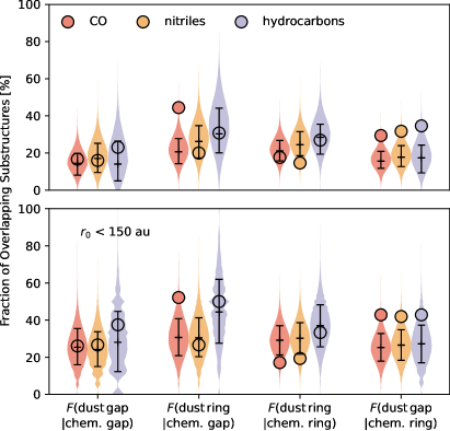
Figure 2: top: Fraction of line-emission substructures that spatially overlap with continuum substructures in each chemical species group.
bottom: The same as the top but only counting line-emission substructures with radial locations $<$150 au.
Circles are observational results. Colored violin plots show the PDF of null hypothesis (line-emission substructures follow random distribution independent of continuum). The error bars show the $[15.9,50,84.1]$ percentiles of the probability distribution.

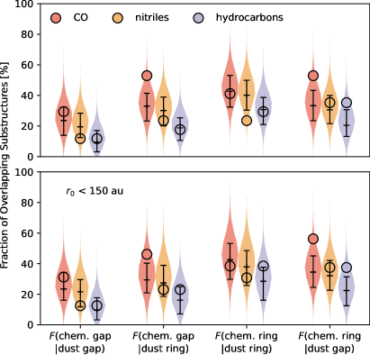
Figure 3: top: Fraction of continuum substructures that spatially overlap with line-emission substructures in each chemical species group.
bottom: The same as the top but only counting line-emission substructures with radial locations $<$150 au.
Circles are observational results. Colored violin plots show the PDF of null hypothesis (line-emission substructures follow random distribution independent of continuum). The error bars show the $[15.9,50,84.1]$ percentiles of the probability distribution.

We find that statistically there is no significant evidence for a universal correlation between line-emission and continuum substructures. That is, the presence of a line-emission substructure does not enhance the probability of finding a dust ring (or gap) in its vicinity. More than half of the observed overlap fractions show statistical significances of ${<}1\sigma$. For individual disks, the observed overlap fractions all fall within the $2\sigma$ ranges of the corresponding PDFs from simulations, except for the overlap fractions, $F(\rm dust\,gap|chemical\,ring)$, of MWC 480 (${>}4\sigma$) and GM Aur ($2.5\sigma$). When all disks are combined, there seems to be a statistically significant (${\sim}4\sigma$) correlation between chemical rings and dust gaps. However, such a detection is primarily driven by the single system of MWC 480. Specifically, there are 13 chemical rings located inside the D76 dust gap in MWC 480, making up one third of the (chem. ring, dust gap) associations of all five disks. If the MWC 480 system is removed from the analysis, the statistical significance of $F(\rm dust|chem.)$ is reduced to below $3\sigma$. Therefore, we conclude that there is no universal correlation between chemical rings and dust gaps.

2.3 Group by chemical species

Even though line-emission substructures as a whole are distributed randomly for most disks, it is still possible that specific molecular lines may correlate with dust rings or gaps more strongly than others. For example, if a certain molecule X triggers the formation of a continuum ring or gap, it may not easily show up in the previous test where substructures from species X are blended with substructures from all other species. We therefore further investigate the $F(\rm dust|chem.)$ by grouping the data with different chemical species. Following Law et al. (2021) (see their Section 3.5), we select and group the chemical species into three groups depending on their chemical similarity—CO isotopologues, nitriles, and hydrocarbons. We collect the chemical features depending on their species group from every disk. Each chemical group is assumed to follow its own random distribution. Therefore, the generation of synthetic systems needs to be modified:

1. For each group of chemical species, the spatial range of the randomly placed substructure spans from the inner- and outer-most locations where substructures from this group of species are detected regardless of disks.

2. For each disk, the number of randomly generated rings/gaps is the same as the number of observed rings/gaps associated with the same group of species. The substructures from different disks are then combined to compute the overlap fraction of the given group of species.

The model parameters are summarized in Table 1. We first calculate $F(\rm dust|chem.)$ and show the results in Fig. 2. Similar to Fig. 1, the open circles indicate the fractions from observations, the violin plots are used to illustrate the PDFs of the fractions derived from the simulation, and the error bars indicate medians and $1\sigma$ ranges. The percentiles of observed overlap are also reported in Table 2.

As shown in Fig. 2 and listed in Table 2, the majority of the observed overlap fractions of the three groups of species are statistically insignificant (${<}3\sigma$), regardless of the combinations of substructures. The only exception is the chemical gap and dust ring alignment in CO isotopologues, which has a statistical significance of $3.3\sigma$ (See Sect. 3). As has been discussed previously, the majority of the line-emission substructures in MWC 480 coincide with the D76 dust gap. This single outlier leads to the marginal detections (${\sim}2\sigma$) of correlations between dust gaps and chemical rings associated with all three groups of species.

By combining the substructures of the same group of species from different disks, we now have a large enough sample to assess the overlap fraction $F(\rm chem.|dust)$. This directly informs the fraction of dust substructures associated with certain chemical species. The results are shown in Fig. 3 and listed in Table 2.

The observed overlap fractions are statistically insignificant (${\lesssim}2\sigma$), regardless of the combination of substructures or the group of chemical species. In other words, the presence of a continuum substructure does not significantly enhance, or decrease, the probability of observing a line-emission substructure in its vicinity. The results are largely unaffected when only substructures within 150 au are included. This analysis strengthens our conclusion that line-emission and dust substructures are generally independent.

3 Conclusion and Discussion

In this work, we revisit the spatial correlation between line-emission and continuum substructures in the MAPS survey. We have calculated the observed overlap fractions of different combinations of substructures for individual disks and individual group of chemical species. We assess the statistical significance by comparing the observed fraction with that from synthetic systems that assume no correlation. Statistically, the current observational results suggest that the line-emission substructures distribution and dust substructures distribution are overall independent of each other. No significant line-emission and continuum substructures correlation is found among the MAPS disks, regardless of accounting for the entire disk or limiting our analysis to the inner 150 au. We report our key findings and briefly discuss them as below:

1. No statistically significant correlation is found between the locations of molecular line emission and dust substructures in at least four out of the five MAPS disks, regardless of which combination of substructure types is considered. In particular, a positive correlation between dust rings and chemical rings is absent. Adopting the simplifying assumption that pressure bumps reflect gas surface density maxima, we would naively expect concomitant peaks in the line emission. Although in reality the actual physical-chemical response to a pressure bump may be more complex such that pressure maxima do not necessarily lead to local chemical emission lines, the lack of a clear continuum–line correlation may alternatively suggest that pressure maxima are perhaps not always the driving mechanism behind continuum rings. If this interpretation is right, it would imply that the gas density profile is smooth around continuum and line substructures. Indeed Alarcón et al. (2021) found that for the AS 209 disk the H₂ gas likely follows a smooth surface-density profile even though there are substructures in certain chemical species.

2. Among the five MAPS systems, MWC 480 is a clear outlier with a significant correlation (${>}4\sigma$) between chemical rings and dust gaps. This strong correlation is primarily due to the large accumulation of line-emission substructures (${>}13$ rings) at its D76 dust gap. Active chemical processing, e.g., gas flow onto the accreting planet(s) (e.g. Liu et al., 2019; Dong et al., 2019; Teague et al., 2019), could be ongoing inside the D76 dust gap in MWC 480.

3. In addition, a weak (${\sim}2\sigma$) trend of association between line-emission rings and dust gaps appears when focusing on CO isotopologues. This meets the scenario demonstrated by some physical-chemical modeling, where the CO emission is increased inside the gaps due to the combination of increased temperature (e.g. van der Marel et al., 2018a; Kim et al., 2020) and contributions of the backside of the disk (e.g. Rab et al., 2020). Specifically, Rab et al. (2020) reproduce this association for both CO 2-1 and C¹⁸O 2-1 emission around the D49 continuum gap in HD 163296. Similar processes may operate in GM Aur to produce the observed trend(${\sim}2.5\sigma$) between dust gaps and CO isotopologues rings.

4. We report a moderate (${\sim}3\sigma$) correlation between line-emission gaps of CO isotopologues and continuum rings. One possible general explanation has been highlighted by Law et al. (2021)—the overdense regions of dust particles may absorb the optically thick lines and lead to gaps in molecular line observations (see also Weaver et al. 2018). A naive expectation of this mechanism would be that the same correlation should get stronger with closer-in substructures, because the regions closer to the star should preferentially be optically thicker (Bosman et al., 2021). This is not observed in our results. In fact, the significance of the same correlation decreases when we only count substructures within 150 au. Another explanation is that excess cooling of grains inside the dust ring can cause a temperature dip and may lead to a line-emission gap (see Sec. 5.2 of Zhang et al., 2021b). Furthermore, optically thick dust rings can absorb the line emission from the back side of the disk (Rab et al., 2020). However, both of these two mechanisms should apply to other species rather than only CO. Finally, with the concentration of pebbles at the midplane, more efficient physical sequestration of CO onto pebbles and local chemical processing may happen inside continuum rings, which could contribute to such a correlation (See Krijt et al. 2020 for a more comprehensive study on CO depletion). More data is needed to confirm this correlation and further analysis and modeling are required to understand its cause.

Given the limitations of current resolution and sample size, one cannot rule out the possibility that some spatial correlations between chemical and dust features may hold for specific disks or specific chemical species. Better conclusions require higher resolution and a larger sample. There is increasing evidence that the current chemical inventory in disks may be strongly affected by dust transport, which will lead to significant correlation between chemical components and continuum disk globally (e.g. Bosman & Banzatti, 2019; Banzatti et al., 2020; van der Marel et al., 2021). Yet, at present, a universal local continuum–emission-line correlation does not stand.

References

- Alarcón et al. (2021) Alarcón, F., Bosman, A. D., Bergin, E. A., et al. 2021, ApJS, 257, 8, doi: 10.3847/1538-4365/ac22ae
- ALMA Partnership et al. (2015) ALMA Partnership, Brogan, C. L., Pérez, L. M., et al. 2015, ApJ, 808, L3, doi: 10.1088/2041-8205/808/1/L3
- Andrews (2020) Andrews, S. M. 2020, ARA&A, 58, 483, doi: 10.1146/annurev-astro-031220-010302
- Andrews et al. (2018) Andrews, S. M., Huang, J., Pérez, L. M., et al. 2018, ApJ, 869, L41, doi: 10.3847/2041-8213/aaf741
- Bai & Stone (2014) Bai, X.-N., & Stone, J. M. 2014, ApJ, 796, 31, doi: 10.1088/0004-637X/796/1/31
- Banzatti et al. (2020) Banzatti, A., Pascucci, I., Bosman, A. D., et al. 2020, ApJ, 903, 124, doi: 10.3847/1538-4357/abbc1a
- Boehler et al. (2017) Boehler, Y., Weaver, E., Isella, A., et al. 2017, ApJ, 840, 60, doi: 10.3847/1538-4357/aa696c
- Bosman & Banzatti (2019) Bosman, A. D., & Banzatti, A. 2019, A&A, 632, L10, doi: 10.1051/0004-6361/201936638
- Bosman et al. (2021) Bosman, A. D., Bergin, E. A., Loomis, R. A., et al. 2021, ApJS, 257, 15, doi: 10.3847/1538-4365/ac1433
- Cieza et al. (2019) Cieza, L. A., Ruíz-Rodríguez, D., Hales, A., et al. 2019, MNRAS, 482, 698, doi: 10.1093/mnras/sty2653
- Dong et al. (2019) Dong, R., Liu, S.-Y., & Fung, J. 2019, ApJ, 870, 72, doi: 10.3847/1538-4357/aaf38e
- Dong et al. (2017) Dong, R., van der Marel, N., Hashimoto, J., et al. 2017, ApJ, 836, 201, doi: 10.3847/1538-4357/aa5abf
- Dullemond et al. (2018) Dullemond, C. P., Birnstiel, T., Huang, J., et al. 2018, ApJ, 869, L46, doi: 10.3847/2041-8213/aaf742
- Facchini et al. (2021) Facchini, S., Teague, R., Bae, J., et al. 2021, AJ, 162, 99, doi: 10.3847/1538-3881/abf0a4
- Fedele et al. (2017) Fedele, D., Carney, M., Hogerheijde, M. R., et al. 2017, A&A, 600, A72, doi: 10.1051/0004-6361/201629860
- Flock et al. (2015) Flock, M., Ruge, J. P., Dzyurkevich, N., et al. 2015, A&A, 574, A68, doi: 10.1051/0004-6361/201424693
- Francis & van der Marel (2020) Francis, L., & van der Marel, N. 2020, ApJ, 892, 111, doi: 10.3847/1538-4357/ab7b63
- Harris et al. (2020) Harris, C. R., Millman, K. J., van der Walt, S. J., et al. 2020, Nature, 585, 357, doi: 10.1038/s41586-020-2649-2
- Huang et al. (2018) Huang, J., Andrews, S. M., Dullemond, C. P., et al. 2018, ApJ, 869, L42, doi: 10.3847/2041-8213/aaf740
- Huang et al. (2020) —. 2020, ApJ, 891, 48, doi: 10.3847/1538-4357/ab711e
- Hunter (2007) Hunter, J. D. 2007, Computing in Science and Engineering, 9, 90, doi: 10.1109/MCSE.2007.55
- Jiang & Ormel (2021) Jiang, H., & Ormel, C. W. 2021, MNRAS, 505, 1162, doi: 10.1093/mnras/stab1278
- Kim et al. (2020) Kim, S., Takahashi, S., Nomura, H., et al. 2020, ApJ, 888, 72, doi: 10.3847/1538-4357/ab5d2b
- Krijt et al. (2020) Krijt, S., Bosman, A. D., Zhang, K., et al. 2020, ApJ, 899, 134, doi: 10.3847/1538-4357/aba75d
- Law et al. (2021) Law, C. J., Loomis, R. A., Teague, R., et al. 2021, ApJS, 257, 3, doi: 10.3847/1538-4365/ac1434
- Lin & Papaloizou (1986) Lin, D. N. C., & Papaloizou, J. 1986, ApJ, 309, 846, doi: 10.1086/164653
- Liu et al. (2019) Liu, Y., Dipierro, G., Ragusa, E., et al. 2019, A&A, 622, A75, doi: 10.1051/0004-6361/201834157
- Long et al. (2018) Long, F., Pinilla, P., Herczeg, G. J., et al. 2018, ApJ, 869, 17, doi: 10.3847/1538-4357/aae8e1
- Öberg et al. (2021) Öberg, K. I., Guzmán, V. V., Walsh, C., et al. 2021, ApJS, 257, 1, doi: 10.3847/1538-4365/ac1432
- Okuzumi et al. (2016) Okuzumi, S., Momose, M., Sirono, S.-i., Kobayashi, H., & Tanaka, H. 2016, ApJ, 821, 82, doi: 10.3847/0004-637X/821/2/82
- Pinilla et al. (2012) Pinilla, P., Benisty, M., & Birnstiel, T. 2012, A&A, 545, A81, doi: 10.1051/0004-6361/201219315
- Rab et al. (2020) Rab, C., Kamp, I., Dominik, C., et al. 2020, A&A, 642, A165, doi: 10.1051/0004-6361/202038712
- Teague et al. (2019) Teague, R., Bae, J., & Bergin, E. A. 2019, Nature, 574, 378, doi: 10.1038/s41586-019-1642-0
- Tominaga et al. (2020) Tominaga, R. T., Takahashi, S. Z., & Inutsuka, S.-i. 2020, ApJ, 900, 182, doi: 10.3847/1538-4357/abad36
- van der Marel et al. (2021) van der Marel, N., Bosman, A. D., Krijt, S., Mulders, G. D., & Bergner, J. B. 2021, A&A, 653, L9, doi: 10.1051/0004-6361/202141786
- van der Marel et al. (2019) van der Marel, N., Dong, R., di Francesco, J., Williams, J. P., & Tobin, J. 2019, ApJ, 872, 112, doi: 10.3847/1538-4357/aafd31
- van der Marel et al. (2016) van der Marel, N., van Dishoeck, E. F., Bruderer, S., et al. 2016, A&A, 585, A58, doi: 10.1051/0004-6361/201526988
- van der Marel et al. (2018a) van der Marel, N., Williams, J. P., & Bruderer, S. 2018a, ApJ, 867, L14, doi: 10.3847/2041-8213/aae88e
- van der Marel et al. (2018b) van der Marel, N., Williams, J. P., Ansdell, M., et al. 2018b, ApJ, 854, 177, doi: 10.3847/1538-4357/aaaa6b
- Virtanen et al. (2020) Virtanen, P., Gommers, R., Oliphant, T. E., et al. 2020, Nature Methods, 17, 261, doi: 10.1038/s41592-019-0686-2
- Weaver et al. (2018) Weaver, E., Isella, A., & Boehler, Y. 2018, ApJ, 853, 113, doi: 10.3847/1538-4357/aaa481
- Zhang et al. (2015) Zhang, K., Blake, G. A., & Bergin, E. A. 2015, ApJ, 806, L7, doi: 10.1088/2041-8205/806/1/L7
- Zhang et al. (2021a) Zhang, K., Booth, A. S., Law, C. J., et al. 2021a, ApJS, 257, 5, doi: 10.3847/1538-4365/ac1580
- Zhang et al. (2021b) Zhang, S., Hu, X., Zhu, Z., & Bae, J. 2021b, ApJ, 923, 70, doi: 10.3847/1538-4357/ac2c82