A novel locking-free virtual element method for linear elasticity problems

Jianguo Huang jghuang@sjtu.edu.cn Sen Lin sjtu_Einsteinlin7@sjtu.edu.cn Yue Yu terenceyuyue@sjtu.edu.cn School of Mathematical Sciences, and MOE-LSC, Shanghai Jiao Tong University, Shanghai 200240, China Institute of Natural Sciences, Shanghai Jiao Tong University, Shanghai 200240, China
Abstract

This paper devises a novel lowest-order conforming virtual element method (VEM) for planar linear elasticity with the pure displacement/traction boundary condition. The main trick is to view a generic polygon K𝐾K as a new one K~~𝐾\widetilde{K} with additional vertices consisting of interior points on edges of K𝐾K, so that the discrete admissible space is taken as the V1subscript𝑉1V_{1} type virtual element space related to the partition {K~}~𝐾\{\widetilde{K}\} instead of {K}𝐾\{K\}. The method is shown to be uniformly convergent with the optimal rates both in H1superscript𝐻1H^{1} and L2superscript𝐿2L^{2} norms with respect to the Lamé constant λ𝜆\lambda. Numerical tests are presented to illustrate the good performance of the proposed VEM and confirm the theoretical results.

keywords:
Virtual element method, Linear elasticity, Locking-free, Numerical tests.
hjgfootnotehjgfootnotefootnotetext: The work of this author was partially supported by NSFC (Grant No. 12071289).

1 Introduction

Robust numerical solution of parameter dependent partial differential equations (PDEs) is a very important topic in scientific computing. A typical example is the linear elasticity problem which involves the Lamé constants λ𝜆\lambda and μ𝜇\mu. If λ𝜆\lambda is very large, the material becomes nearly incompressible, which will lead to the so-called volume locking phenomenon when the Courant element is used for discretization (cf. [9]). Because of this, a huge work has been developed to overcome this difficulty. We refer the reader to [7, 8, 16, 18, 20, 28, 29, 32, 38, 41] and the references therein for details along this line.

On the other hand, the virtual element method (VEM) is a newly proposed numerical method for solving PDEs in recent years, which can be viewed as a generalized finite element method allowing for the use of polytopal meshes (polygons or polyhedra) of very general shape. It was first proposed and analyzed in [3, 10, 12] and immediately attracted much attention from the research community due to its advantages in handling problems with complex geometries, high-regularity solutions (cf. [22, 31]). As far as we know, there have also developed some locking free VEMs for the linear elasticity problem. Let k𝑘k denote the order of the virtual element used. The conforming VEMs for this problem were first studied in [11]. However, the condition k2𝑘2k\geq 2 is required so as to produce locking free optimal error estimates in the H1superscript𝐻1H^{1} norm. More recently, a lowest-order locking-free VEM was devised in [37] to remedy this disadvantage by modifying the W1subscript𝑊1W_{1} type virtual element technically so that the uniform inf-sup condition holds. This method can be regarded as the extension of the well-known Bernardi-Raugel finite element method (cf. [15]) in general polygonal meshes. In [40], some nonconforming VEMs were proposed for attacking the previous problem in two and three dimensions. It was shown in this paper that if k1𝑘1k\geq 1 (resp. k2𝑘2k\geq 2), the method is locking-free for the pure displacement (resp. traction) problem. We mention in passing that there are some other VEMs discussing numerical solution of elasticity problems in different aspects; see, e.g., [1, 4, 5, 6, 14, 19, 24, 26, 27, 33, 34, 35, 39].

In this paper, we are concerned with proposing and analyzing a novel lowest-order conforming locking-free VEM for the pure dispalcement/traction problem, by means of a significant feature of VEMs. The main ideas behind the method include:

  1. 1.

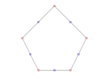
    For a generic polygonal element K𝐾K with NKsubscript𝑁𝐾N_{K} edges, denoted by {zi}i=1NKsuperscriptsubscriptsubscript𝑧𝑖𝑖1subscript𝑁𝐾\{z_{i}\}_{i=1}^{N_{K}} its vertices which are numbered in a counter-clockwise order and by ei=zizi+1¯subscript𝑒𝑖¯subscript𝑧𝑖subscript𝑧𝑖1e_{i}=\overline{z_{i}z_{i+1}} the edge connecting zisubscript𝑧𝑖z_{i} to zi+1subscript𝑧𝑖1z_{i+1}, where zNK+1:=z1assignsubscript𝑧subscript𝑁𝐾1subscript𝑧1z_{N_{K}+1}:=z_{1}. Then we construct an auxiliary polygon K~~𝐾\widetilde{K} (see Fig. 1), which has the same geometric shape as K𝐾K but has more vertices. Precisely speaking, besides the vertices of K𝐾K, K~~𝐾\widetilde{K} has additional vertices formed by the internal points {mi}i=1NKsuperscriptsubscriptsubscript𝑚𝑖𝑖1subscript𝑁𝐾\{m_{i}\}_{i=1}^{N_{K}} of edges of K𝐾K, which are chosen such that |zimi¯|=α|zizi+1¯|¯subscript𝑧𝑖subscript𝑚𝑖𝛼¯subscript𝑧𝑖subscript𝑧𝑖1|\overline{z_{i}m_{i}}|=\alpha|\overline{z_{i}z_{i+1}}|, where α(0,1)𝛼01\alpha\in(0,1) is any fixed constant. It is a significant advantage of VEMs that one can view an interior point of an edge as an additional vertex, so that the difficulty of hanging nodes during adaptivity can be overcome very conveniently (cf. [30]). But here we use the technique to construct locking free VEMs.

  2. 2.

    Based on the V1subscript𝑉1V_{1} type virtual element space with respect the partition {K~}~𝐾\{\widetilde{K}\} instead of the usual one {K}𝐾\{K\}, a locking free VEM is naturally devised using the ideas in [11] for k2𝑘2k\geq 2.

Under the standard mesh assumption C0 (see Subsection 3.1), we can show the proposed method is locking free and has the optimal convergence order by invoking a novel interpolation operator which satisfies the required commutative property and admits the optimal error estimates. We offer several numerical tests to illustrate the performance of the proposed method and confirm its theoretical predictions.

We end this section by introducing some notations for later requirement. We use standard notations for Sobolev spaces and norms (see [2] for more details). Let D𝐷D be any open subset of ΩΩ\Omega and |D|𝐷|D| denote the area of D𝐷D. Given a non-negative integer s𝑠s, we denote the standard Sobolev spaces on D𝐷D by Hs(D)superscript𝐻𝑠𝐷H^{s}(D) with norm s,D\|\cdot\|_{s,D} and semi-norm ||s,D|\cdot|_{s,D}, and denote the L2superscript𝐿2L^{2}-inner product on D𝐷D by (,)Dsubscript𝐷(\cdot,\,\cdot)_{D}. By convention, H0(D)=L2(D)superscript𝐻0𝐷superscript𝐿2𝐷H^{0}(D)=L^{2}(D). Let s(D)subscript𝑠𝐷\mathbb{P}_{s}(D) be the set of polynomials of degree less than s𝑠s on D𝐷D. Moreover, we omit the subscript when D=Ω𝐷ΩD=\Omega. For the vector-valued functions or spaces, we use the bold symbols, such as 𝒗𝒗\boldsymbol{v}, 𝑳2(Ω)superscript𝑳2Ω\boldsymbol{L}^{2}(\Omega), 𝑯s(Ω)superscript𝑯𝑠Ω\boldsymbol{H}^{s}(\Omega), 𝑯0s(Ω)superscriptsubscript𝑯0𝑠Ω\boldsymbol{H}_{0}^{s}(\Omega), etc. Let 𝒗=(v1,v2)𝒗superscriptsubscript𝑣1subscript𝑣2\boldsymbol{v}=(v_{1},\,v_{2})^{\intercal} and 𝝉=[τij]2×2𝝉subscriptdelimited-[]subscript𝜏𝑖𝑗22\boldsymbol{\tau}=[\tau_{ij}]_{2\times 2} be functions of two variables. We define

div𝒗=1v1+2v2,rot𝒗=1v22v1,and𝐝𝐢𝐯𝝉=(1τ11+2τ12,1τ21+2τ22).formulae-sequencediv𝒗subscript1subscript𝑣1subscript2subscript𝑣2formulae-sequencerot𝒗subscript1subscript𝑣2subscript2subscript𝑣1and𝐝𝐢𝐯𝝉superscriptsubscript1subscript𝜏11subscript2subscript𝜏12subscript1subscript𝜏21subscript2subscript𝜏22\displaystyle{\rm{div}}~{}\boldsymbol{v}=\partial_{1}{v}_{1}+\partial_{2}{v}_{2},\quad{\rm{rot}}~{}\boldsymbol{v}=\partial_{1}{v}_{2}-\partial_{2}{v}_{1},\quad\text{and}\quad\boldsymbol{\rm{div}~{}\boldsymbol{\tau}}=(\partial_{1}{\tau_{11}}+\partial_{2}{\tau_{12}},\partial_{1}{\tau_{21}}+\partial_{2}{\tau_{22}})^{\intercal}.

For any two quantities a𝑎a and b𝑏b, “abless-than-or-similar-to𝑎𝑏a\lesssim b” indicates “aCb𝑎𝐶𝑏a\leq Cb” with the hidden generic positive constant C𝐶C independent of λ𝜆\lambda and the mesh size, which may take different values at different occurrences, and ab𝑎𝑏a\eqsim b shows abaless-than-or-similar-to𝑎𝑏less-than-or-similar-to𝑎a\lesssim b\lesssim a.

2 The linear elasticity problem

Let Ω2Ωsuperscript2\Omega\subset\mathbb{R}^{2} be a convex polygonal domain with the boundary ΩΩ\partial\Omega. Given an applied force 𝒇𝑳2(Ω)𝒇superscript𝑳2Ω\boldsymbol{f}\in\boldsymbol{L}^{2}(\Omega), the linear elasticity problem is to find the displacement vector 𝒖=(u1,u2)𝒖superscriptsubscript𝑢1subscript𝑢2\boldsymbol{u}=(u_{1},\,u_{2})^{\intercal} such that

{𝐝𝐢𝐯𝝈(𝒖)=𝒇inΩ,𝒖=𝟎onΩ,cases𝐝𝐢𝐯𝝈𝒖𝒇inΩ𝒖0onΩ\begin{cases}-\boldsymbol{\rm div}~{}\boldsymbol{\sigma}(\boldsymbol{u})=\boldsymbol{f}&\text{in}~{}~{}\Omega,\\ \boldsymbol{u}=\boldsymbol{0}&\text{on}~{}~{}\partial\Omega,\end{cases} (2.1)

where 𝜺=[εij]2×2𝜺subscriptdelimited-[]subscript𝜀𝑖𝑗22\boldsymbol{\varepsilon}=[\varepsilon_{ij}]_{2\times 2}, εij(𝒖)=12(iuj+jui)subscript𝜀𝑖𝑗𝒖12subscript𝑖subscript𝑢𝑗subscript𝑗subscript𝑢𝑖\varepsilon_{ij}(\boldsymbol{u})=\frac{1}{2}(\partial_{i}u_{j}+\partial_{j}u_{i}), and

𝝈=2μ𝜺(𝒖)+λ(div𝒖)𝑰.𝝈2𝜇𝜺𝒖𝜆div𝒖𝑰\boldsymbol{\sigma}=2\mu\boldsymbol{\varepsilon}(\boldsymbol{u})+\lambda({\rm div}~{}\boldsymbol{u})\boldsymbol{I}.

Here, μ𝜇\mu and λ𝜆\lambda are the Lamé constants satisfying μ[μ1,μ2]𝜇subscript𝜇1subscript𝜇2\mu\in[\mu_{1},\mu_{2}] with 0<μ1<μ20subscript𝜇1subscript𝜇20<\mu_{1}<\mu_{2} and λ(0,)𝜆0\lambda\in(0,\infty), and 𝑰𝑰\boldsymbol{I} is the identity matrix.

The variational formulation of (2.1) is to find 𝒖𝑽=𝑯01(Ω)𝒖𝑽superscriptsubscript𝑯01Ω\boldsymbol{u}\in\boldsymbol{V}=\boldsymbol{H}_{0}^{1}(\Omega) such that

a(𝒖,𝒗)=(𝒇,𝒗),𝒗𝑽,formulae-sequence𝑎𝒖𝒗𝒇𝒗𝒗𝑽a(\boldsymbol{u},\,\boldsymbol{v})=(\boldsymbol{f},\,\boldsymbol{v}),\quad\boldsymbol{v}\in\boldsymbol{V}, (2.2)

where

a(𝒘,𝒗)=2μ(𝜺(𝒘),𝜺(𝒗))+λ(div𝒘,div𝒗),𝒘,𝒗𝑽,formulae-sequence𝑎𝒘𝒗2𝜇𝜺𝒘𝜺𝒗𝜆div𝒘div𝒗𝒘𝒗𝑽a(\boldsymbol{w},\,\boldsymbol{v})=2\mu(\boldsymbol{\varepsilon}(\boldsymbol{w}),\,\boldsymbol{\varepsilon}(\boldsymbol{v}))+\lambda({\rm div}~{}\boldsymbol{w},\,{\rm div}~{}\boldsymbol{v}),\quad\boldsymbol{w},\boldsymbol{v}\in\boldsymbol{V}, (2.3)

and

(𝒇,𝒗)=Ω𝒇𝒗dx,𝒗𝑽.formulae-sequence𝒇𝒗subscriptΩ𝒇𝒗differential-d𝑥𝒗𝑽(\boldsymbol{f},\,\boldsymbol{v})=\int_{\Omega}\boldsymbol{f}\boldsymbol{v}\,\mathrm{d}x,\quad\boldsymbol{v}\in\boldsymbol{V}.

By the well-known Korn inequality (cf. [17]):

𝒗1𝜺(𝒗)0,𝒗𝑯01(Ω),formulae-sequenceless-than-or-similar-tosubscriptnorm𝒗1subscriptnorm𝜺𝒗0𝒗superscriptsubscript𝑯01Ω\displaystyle\|\boldsymbol{v}\|_{1}\lesssim\|\boldsymbol{\varepsilon}(\boldsymbol{v})\|_{0},\quad\boldsymbol{v}\in\boldsymbol{H}_{0}^{1}(\Omega), (2.4)

it is easy to obtain the boundedness and coercivity of a(,)𝑎a(\cdot,\,\cdot):

a(𝒘,𝒗)𝑎𝒘𝒗\displaystyle a(\boldsymbol{w},\,\boldsymbol{v}) (1+λ)|𝒘|1|𝒗|1,𝒘,𝒗𝑽,formulae-sequenceless-than-or-similar-toabsent1𝜆subscript𝒘1subscript𝒗1𝒘𝒗𝑽\displaystyle\lesssim(1+\lambda)|\boldsymbol{w}|_{1}|\boldsymbol{v}|_{1},\quad\boldsymbol{w},\boldsymbol{v}\in\boldsymbol{V},
|𝒗|12superscriptsubscript𝒗12\displaystyle|\boldsymbol{v}|_{1}^{2} a(𝒗,𝒗),𝒗𝑽,formulae-sequenceless-than-or-similar-toabsent𝑎𝒗𝒗𝒗𝑽\displaystyle\lesssim a(\boldsymbol{v},\,\boldsymbol{v}),\quad\boldsymbol{v}\in\boldsymbol{V},

which imply that the problem (2.1) has a unique solution by the Lax-Milgram lemma.

Since the first term of a(,)𝑎a(\cdot,\cdot) (cf. (2.3)) is related to μ𝜇\mu, we write

aμ(𝒘,𝒗)=(𝜺(𝒘),𝜺(𝒗))subscript𝑎𝜇𝒘𝒗𝜺𝒘𝜺𝒗a_{\mu}(\boldsymbol{w},\boldsymbol{v})=(\boldsymbol{\varepsilon}(\boldsymbol{w}),\,\boldsymbol{\varepsilon}(\boldsymbol{v}))

for later uses.

It is shown in [18] that the following regularity estimate holds for the solution 𝒖𝒖\boldsymbol{u} of (2.1):

𝒖2+λdiv𝒖1𝒇0.less-than-or-similar-tosubscriptnorm𝒖2𝜆subscriptnormdiv𝒖1subscriptnorm𝒇0\|\boldsymbol{u}\|_{2}+\lambda\|{\rm div}~{}\boldsymbol{u}\|_{1}\lesssim\|\boldsymbol{f}\|_{0}. (2.5)

3 Virtual element methods for the pure displacement problem

In this section, by means of a mesh refinement trick in VEMs, we propose a novel lowest order locking-free conforming virtual element method on the fine mesh.

3.1 Mesh assumption and the virtual element space

Let {𝒯h}subscript𝒯\{\mathcal{T}_{h}\} be a family of decompositions of ΩΩ\Omega into polygonal elements. The generic element is denoted by K𝐾K with diameter hK=diam(K)subscript𝐾diam𝐾h_{K}={\rm diam}(K). For clarity, we work on meshes satisfying the following condition (cf. [10]):

  1. C0.

    For each element K𝐾K, there exists positive constants γ1subscript𝛾1\gamma_{1} and γ2subscript𝛾2\gamma_{2} independent of hKsubscript𝐾h_{K} such that

    • (a)

      K𝐾K is star-shaped with respect to a disc in K𝐾K with radius γ1hKabsentsubscript𝛾1subscript𝐾\geq\gamma_{1}{h_{K}};

    • (b)

      the distance between any two vertices of K𝐾K is γ2hKabsentsubscript𝛾2subscript𝐾\geq\gamma_{2}h_{K}.

Refer to caption
Fig. 1: The auxiliary polygon K~~𝐾\widetilde{K} satisfying the mesh assumption C0. The polygonal elements of the fine mesh 𝒯hsuperscriptsubscript𝒯\mathcal{T}_{h}^{*} and the original mesh 𝒯hsubscript𝒯\mathcal{T}_{h} are denoted by K~~𝐾\widetilde{K} and K𝐾K, respectively. The red circle points denote the original vertices, the blue square points denote the added vertices.

Due to the large flexibility of the meshes in VEMs, under the above assumption, one easily finds that the mesh can be refined by taking the internal point misubscript𝑚𝑖m_{i} of each edge eisubscript𝑒𝑖e_{i} of every element K𝐾K as a new vertex (see Fig. 1). For the new edge |zimi¯|¯subscript𝑧𝑖subscript𝑚𝑖|\overline{z_{i}m_{i}}|, we assume |zimi¯|=α|ei|¯subscript𝑧𝑖subscript𝑚𝑖𝛼subscript𝑒𝑖|\overline{z_{i}m_{i}}|=\alpha|e_{i}| for i=1,2,,NK𝑖12subscript𝑁𝐾i=1,2,\ldots,N_{K} for a given constant α(0,1)𝛼01\alpha\in(0,1). The resulting fine mesh will be denoted by 𝒯hsuperscriptsubscript𝒯\mathcal{T}_{h}^{*} with the generic element given by K~~𝐾\widetilde{K}. It’s obvious that 𝒯hsuperscriptsubscript𝒯\mathcal{T}_{h}^{*} still satisfies the assumption C0 thought the generic constants may change. Here, h=maxK~𝒯hhK~subscript~𝐾superscriptsubscript𝒯subscript~𝐾h=\max_{\widetilde{K}\in\mathcal{T}_{h}^{*}}h_{\widetilde{K}} with hK~subscript~𝐾h_{\widetilde{K}} being the diameter of K~~𝐾\widetilde{K}. It is evident that hKhK~subscript𝐾subscript~𝐾h_{K}\eqsim h_{\widetilde{K}}.

In this paper, we consider the lowest-order conforming virtual element space (VES) defined on the fine mesh 𝒯hsuperscriptsubscript𝒯\mathcal{T}_{h}^{*}. To this end, we briefly review the construction method mentioned in [10]. The local scalar virtual element space on K~~𝐾\widetilde{K} is defined as

V1(K~)={vH1(K~)|Δv=0inK~,v|e1(e),eK~}.subscript𝑉1~𝐾conditional-set𝑣superscript𝐻1~𝐾formulae-sequenceΔ𝑣0in~𝐾formulae-sequenceevaluated-at𝑣𝑒subscript1𝑒𝑒~𝐾V_{1}(\widetilde{K})=\big{\{}v\in H^{1}(\widetilde{K})~{}|~{}\Delta v=0~{}~{}\mbox{in}~{}~{}\widetilde{K},~{}v|_{e}\in\mathbb{P}_{1}(e),\quad e\subset\partial{\widetilde{K}}\big{\}}. (3.1)

The local virtual element space for linear elasticity is then given by the tensor product space 𝑽1(K~)=(V1(K~))2subscript𝑽1~𝐾superscriptsubscript𝑉1~𝐾2\boldsymbol{V}_{1}(\widetilde{K})=(V_{1}(\widetilde{K}))^{2}. The corresponding local degrees of freedoms (DOFs) are:

  • 1.

    χi𝝌subscript𝜒𝑖𝝌\chi_{i}\in\boldsymbol{\chi}: the values at vertices of K~~𝐾\widetilde{K},

    χi(𝒗)=𝒗(ai),where ai=zi or mi is the vertex of K~.subscript𝜒𝑖𝒗𝒗subscript𝑎𝑖where ai=zi or mi is the vertex of K~\chi_{i}(\boldsymbol{v})=\boldsymbol{v}(a_{i}),\quad\mbox{where~{}$a_{i}=z_{i}$~{}or~{}$m_{i}$~{}is the vertex of ~{}$\widetilde{K}$}.

In what follows, denote by 𝑽hsubscript𝑽\boldsymbol{V}_{h} the global VES, which is defined elementwise and required that the degrees of freedom are continuous through the interior vertices while zero for the boundary DOFs, i.e.,

𝑽h={𝒗𝑯01(Ω)|𝒗|K~𝑽1(K~),K~𝒯h}.subscript𝑽conditional-set𝒗superscriptsubscript𝑯01Ωformulae-sequenceevaluated-at𝒗~𝐾subscript𝑽1~𝐾~𝐾superscriptsubscript𝒯\displaystyle\boldsymbol{V}_{h}=\big{\{}\boldsymbol{v}\in\boldsymbol{H}_{0}^{1}(\Omega)~{}|~{}\boldsymbol{v}|_{\widetilde{K}}\in\boldsymbol{V}_{1}(\widetilde{K}),\quad\widetilde{K}\in\mathcal{T}_{h}^{*}\big{\}}.

3.2 The virtual element method

As in [11], we first introduce the elliptic projection Π1K~:𝑯1(K~)(1(K~))2:superscriptsubscriptΠ1~𝐾superscript𝑯1~𝐾superscriptsubscript1~𝐾2{\Pi}_{1}^{\widetilde{K}}\colon\boldsymbol{H}^{1}(\widetilde{K})\to(\mathbb{P}_{1}(\widetilde{K}))^{2} for dealing with the first term of (2.3), which is given by

{(𝜺(Π1K~𝒗),𝜺(𝒑))K~=(𝜺(𝒗),𝜺(𝒑))K~,𝒑(1(K~))2,K~Π1K~𝒗ds=K~𝒗ds,K~rotΠ1K~𝒗dx=K~rot𝒗dx.casesformulae-sequencesubscript𝜺superscriptsubscriptΠ1~𝐾𝒗𝜺𝒑~𝐾subscript𝜺𝒗𝜺𝒑~𝐾𝒑superscriptsubscript1~𝐾2otherwisesubscript~𝐾superscriptsubscriptΠ1~𝐾𝒗differential-d𝑠subscript~𝐾𝒗differential-d𝑠otherwisesubscript~𝐾rotsuperscriptsubscriptΠ1~𝐾𝒗differential-d𝑥subscript~𝐾rot𝒗differential-d𝑥otherwise\begin{cases}(\boldsymbol{\varepsilon}({\Pi}_{1}^{\widetilde{K}}\boldsymbol{v}),\,\boldsymbol{\varepsilon}(\boldsymbol{p}))_{\widetilde{K}}=(\boldsymbol{\varepsilon}(\boldsymbol{v}),\,\boldsymbol{\varepsilon}(\boldsymbol{p}))_{\widetilde{K}},\quad\boldsymbol{p}\in(\mathbb{P}_{1}(\widetilde{K}))^{2},\\ \int_{\partial{\widetilde{K}}}{\Pi}_{1}^{\widetilde{K}}\boldsymbol{v}\,\mathrm{d}s=\int_{\partial{\widetilde{K}}}\boldsymbol{v}\,\mathrm{d}s,\\ \int_{\widetilde{K}}{\rm{rot}}~{}{\Pi}_{1}^{\widetilde{K}}\boldsymbol{v}\,\mathrm{d}x=\int_{\widetilde{K}}{\rm{rot}}~{}\boldsymbol{v}\,\mathrm{d}x.\end{cases} (3.2)

One can check that the elliptic projection Π1K~superscriptsubscriptΠ1~𝐾{\Pi}_{1}^{\widetilde{K}} can be computed by the given DOFs. For simplicity, we write Π1subscriptΠ1\Pi_{1} for the related elementwise defined global operator.

Next, Let Π0KsuperscriptsubscriptΠ0𝐾\Pi_{0}^{K} be the usual L2superscript𝐿2L^{2} orthogonal projection from L2(K)superscript𝐿2𝐾L^{2}(K) into the constant space over K𝐾K. In other words, for all vL2(K)𝑣superscript𝐿2𝐾v\in L^{2}(K), Π0Kv=Kvdx/|K|superscriptsubscriptΠ0𝐾𝑣subscript𝐾𝑣differential-d𝑥𝐾\Pi_{0}^{K}v=\int_{K}v\mathrm{d}x/|K|. This definition naturally applies to a L2superscript𝐿2L^{2} vector valued function. For all 𝒗𝑯1(K)𝒗superscript𝑯1𝐾\boldsymbol{v}\in\boldsymbol{H}^{1}(K), by integration by parts,

Kdiv𝒗dx=K𝒗𝒏KdsandKrot𝒗dx=K𝒗𝒕Kds,formulae-sequencesubscript𝐾div𝒗differential-d𝑥subscript𝐾𝒗subscript𝒏𝐾differential-d𝑠andsubscript𝐾rot𝒗differential-d𝑥subscript𝐾𝒗subscript𝒕𝐾differential-d𝑠\int_{K}{\rm div}~{}\boldsymbol{v}\,\mathrm{d}x=\int_{\partial{K}}\boldsymbol{v}\cdot\boldsymbol{n}_{K}\,\mathrm{d}s\quad\mbox{and}\quad\int_{K}{\rm rot}~{}\boldsymbol{v}\,\mathrm{d}x=\int_{\partial{K}}\boldsymbol{v}\cdot\boldsymbol{t}_{K}\,\mathrm{d}s,

where 𝒏K=(n1,n2)subscript𝒏𝐾superscriptsubscript𝑛1subscript𝑛2\boldsymbol{n}_{K}=(n_{1},n_{2})^{\intercal} and 𝒕K=(n2,n1)subscript𝒕𝐾superscriptsubscript𝑛2subscript𝑛1\boldsymbol{t}_{K}=(-n_{2},n_{1})^{\intercal} denote the unit normal and tangent vector to K𝐾\partial{K} determined by the right hand side, respectively. Hence, for all 𝒗𝑽1(K)𝒗subscript𝑽1𝐾\boldsymbol{v}\in\boldsymbol{V}_{1}(K), we can compute Π0Kdiv𝒗superscriptsubscriptΠ0𝐾div𝒗\Pi_{0}^{K}{\rm div}~{}\boldsymbol{v} and Π0Krot𝒗superscriptsubscriptΠ0𝐾rot𝒗\Pi_{0}^{K}{\rm rot}~{}\boldsymbol{v} only using the function values at the vertices of K𝐾K. Therefore, we treat the second term in (2.3) using the exact method for the case k2𝑘2k\geq 2 given in [11].

With the help of the above projections, we construct the local computable bilinear form by

ahK~(𝒘h,𝒗h)=2μaμ,hK~(𝒘h,𝒗h)+λ(Π0Kdiv𝒘h,Π0Kdiv𝒗h)K,𝒘h,𝒗h𝑽1(K~),formulae-sequencesuperscriptsubscript𝑎~𝐾subscript𝒘subscript𝒗2𝜇superscriptsubscript𝑎𝜇~𝐾subscript𝒘subscript𝒗𝜆subscriptsuperscriptsubscriptΠ0𝐾divsubscript𝒘superscriptsubscriptΠ0𝐾divsubscript𝒗𝐾subscript𝒘subscript𝒗subscript𝑽1~𝐾\displaystyle a_{h}^{\widetilde{K}}(\boldsymbol{w}_{h},\,\boldsymbol{v}_{h})=2\mu a_{\mu,h}^{\widetilde{K}}(\boldsymbol{w}_{h},\,\boldsymbol{v}_{h})+\lambda(\Pi_{0}^{K}{\rm div}~{}\boldsymbol{w}_{h},\,\Pi_{0}^{K}{\rm div}~{}\boldsymbol{v}_{h})_{K},\quad\boldsymbol{w}_{h},\boldsymbol{v}_{h}\in\boldsymbol{V}_{1}(\widetilde{K}), (3.3)

where

aμ,hK~(𝒘h,𝒗h)=(𝜺(Π1K~𝒘h),𝜺(Π1K~𝒗h))K~+SK~(𝒘hΠ1K~𝒘h,𝒗hΠ1K~𝒗h)superscriptsubscript𝑎𝜇~𝐾subscript𝒘subscript𝒗subscript𝜺superscriptsubscriptΠ1~𝐾subscript𝒘𝜺superscriptsubscriptΠ1~𝐾subscript𝒗~𝐾superscript𝑆~𝐾subscript𝒘superscriptsubscriptΠ1~𝐾subscript𝒘subscript𝒗superscriptsubscriptΠ1~𝐾subscript𝒗\displaystyle a_{\mu,h}^{\widetilde{K}}(\boldsymbol{w}_{h},\,\boldsymbol{v}_{h})=(\boldsymbol{\varepsilon}(\Pi_{1}^{\widetilde{K}}\boldsymbol{w}_{h}),\,\boldsymbol{\varepsilon}(\Pi_{1}^{\widetilde{K}}\boldsymbol{v}_{h}))_{\widetilde{K}}+S^{\widetilde{K}}(\boldsymbol{w}_{h}-\Pi_{1}^{\widetilde{K}}\boldsymbol{w}_{h},\,\boldsymbol{v}_{h}-\Pi_{1}^{\widetilde{K}}\boldsymbol{v}_{h})

and

SK~(𝒘h,𝒗h)=𝝌(𝒘h)𝝌(𝒗h)=i=1NK~χi(𝒘h)χi(𝒗h)superscript𝑆~𝐾subscript𝒘subscript𝒗𝝌subscript𝒘𝝌subscript𝒗superscriptsubscript𝑖1subscript𝑁~𝐾subscript𝜒𝑖subscript𝒘subscript𝜒𝑖subscript𝒗S^{\widetilde{K}}(\boldsymbol{w}_{h},\,\boldsymbol{v}_{h})=\boldsymbol{\chi}(\boldsymbol{w}_{h})\cdot\boldsymbol{\chi}(\boldsymbol{v}_{h})=\sum\limits_{i=1}^{N_{\widetilde{K}}}\chi_{i}(\boldsymbol{w}_{h})\cdot\chi_{i}(\boldsymbol{v}_{h})

with NK~=2NKsubscript𝑁~𝐾2subscript𝑁𝐾N_{\widetilde{K}}=2N_{K}.

The locking-free conforming VEM of the variational problem (2.2) is to find 𝒖h𝑽hsubscript𝒖subscript𝑽\boldsymbol{u}_{h}\in\boldsymbol{V}_{h} such that

ah(𝒖h,𝒗h)=𝒇h,𝒗h,𝒗h𝑽h,formulae-sequencesubscript𝑎subscript𝒖subscript𝒗subscript𝒇subscript𝒗subscript𝒗subscript𝑽a_{h}(\boldsymbol{u}_{h},\,\boldsymbol{v}_{h})=\langle\boldsymbol{f}_{h},\,\boldsymbol{v}_{h}\rangle,\quad\boldsymbol{v}_{h}\in\boldsymbol{V}_{h}, (3.4)

where

ah(𝒖h,𝒗h)=K𝒯hahK(𝒖h,𝒗h),subscript𝑎subscript𝒖subscript𝒗subscript𝐾subscript𝒯superscriptsubscript𝑎𝐾subscript𝒖subscript𝒗a_{h}(\boldsymbol{u}_{h},\,\boldsymbol{v}_{h})=\sum\limits_{K\in\mathcal{T}_{h}}a_{h}^{K}(\boldsymbol{u}_{h},\,\boldsymbol{v}_{h}),

and the approximation of the right hand side is given by

𝒇h,𝒗h=K~𝒯h(𝒇h,𝒗^h)K~,subscript𝒇subscript𝒗subscript~𝐾superscriptsubscript𝒯subscriptsubscript𝒇subscript^𝒗~𝐾\langle\boldsymbol{f}_{h},\,\boldsymbol{v}_{h}\rangle=\sum_{\widetilde{K}\in\mathcal{T}_{h}^{*}}(\boldsymbol{f}_{h},\,\hat{\boldsymbol{v}}_{h})_{\widetilde{K}}, (3.5)

where 𝒇h|K~=Π0K~𝒇evaluated-atsubscript𝒇~𝐾superscriptsubscriptΠ0~𝐾𝒇\boldsymbol{f}_{h}|_{\widetilde{K}}=\Pi_{0}^{\widetilde{K}}\boldsymbol{f} and

𝒗^h=1|K~|K~𝒗hds.subscript^𝒗1~𝐾subscript~𝐾subscript𝒗differential-d𝑠\hat{\boldsymbol{v}}_{h}=\frac{1}{|\partial{\widetilde{K}}|}\int_{\partial\widetilde{K}}\boldsymbol{v}_{h}\,\mathrm{d}s.
Remark 3.1.

It is worth mentioning that the proposed lowest-order conforming virtual element on triangular meshes is not the well-known Courant element.

3.3 Stability of the virtual element method

We first recall a classic Korn’s inequality with respect to a star-shaped domain.

Lemma 3.1 ([18, 23]).

Let D2𝐷superscript2D\subset\mathbb{R}^{2} be a bounded domain of diameter hh, which is star-shaped with respect to a disc of radius ρ𝜌\rho. Then for any 𝐯𝐇1(D)𝐯superscript𝐇1𝐷\boldsymbol{v}\in\boldsymbol{H}^{1}(D) satisfying Drot𝐯dx=0subscript𝐷rot𝐯differential-d𝑥0\int_{D}{\rm{rot}}~{}\boldsymbol{v}\,\mathrm{d}x=0, there holds

|𝒗|1,D𝜺(𝒗)0,D,less-than-or-similar-tosubscript𝒗1𝐷subscriptnorm𝜺𝒗0𝐷\displaystyle|\boldsymbol{v}|_{1,D}\lesssim\|\boldsymbol{\varepsilon}(\boldsymbol{v})\|_{0,D},

where the hidden constant C𝐶C only depends on the aspect ratio h/ρ𝜌h/\rho.

With the help of the above lemmas, we are able to derive the norm equivalence and the stability condition for the proposed virtual element method (3.4) described as follows.

Theorem 3.1.

Under the mesh assumption C0, for all 𝐯h𝐕hsubscript𝐯subscript𝐕\boldsymbol{v}_{h}\in\boldsymbol{V}_{h} there hold

𝜺(𝒗hΠ1K~𝒗h)0,K~𝝌(𝒗hΠ1K~𝒗h)l2,K~𝒯h,formulae-sequencesubscriptnorm𝜺subscript𝒗superscriptsubscriptΠ1~𝐾subscript𝒗0~𝐾subscriptnorm𝝌subscript𝒗superscriptsubscriptΠ1~𝐾subscript𝒗superscript𝑙2~𝐾superscriptsubscript𝒯\displaystyle\|\boldsymbol{\varepsilon}(\boldsymbol{v}_{h}-\Pi_{1}^{\widetilde{K}}\boldsymbol{v}_{h})\|_{0,\widetilde{K}}\eqsim\|\boldsymbol{\chi}(\boldsymbol{v}_{h}-\Pi_{1}^{\widetilde{K}}\boldsymbol{v}_{h})\|_{l^{2}},\quad\widetilde{K}\in\mathcal{T}_{h}^{*}, (3.6)

and

aμ,hK~(𝒗h,𝒗h)aμK~(𝒗h,𝒗h),K~𝒯h,formulae-sequencesuperscriptsubscript𝑎𝜇~𝐾subscript𝒗subscript𝒗superscriptsubscript𝑎𝜇~𝐾subscript𝒗subscript𝒗~𝐾superscriptsubscript𝒯\displaystyle a_{\mu,h}^{\widetilde{K}}(\boldsymbol{v}_{h},\,\boldsymbol{v}_{h})\eqsim a_{\mu}^{\widetilde{K}}(\boldsymbol{v}_{h},\,\boldsymbol{v}_{h}),\quad\widetilde{K}\in\mathcal{T}_{h}^{*}, (3.7)

where aμK~(𝐯h,𝐯h)superscriptsubscript𝑎𝜇~𝐾subscript𝐯subscript𝐯a_{\mu}^{\widetilde{K}}(\boldsymbol{v}_{h},\,\boldsymbol{v}_{h}) is the local conterpart of aμ(𝐯h,𝐯h)subscript𝑎𝜇subscript𝐯subscript𝐯a_{\mu}(\boldsymbol{v}_{h},\,\boldsymbol{v}_{h}).

Proof.

By the definition of Π1K~superscriptsubscriptΠ1~𝐾\Pi_{1}^{\widetilde{K}} and Lemma 3.1, one has

𝜺(𝒗hΠ1K~𝒗h)0,K~|𝒗hΠ1K~𝒗h|1,K~,𝒗h𝑽h.formulae-sequencesubscriptnorm𝜺subscript𝒗superscriptsubscriptΠ1~𝐾subscript𝒗0~𝐾subscriptsubscript𝒗superscriptsubscriptΠ1~𝐾subscript𝒗1~𝐾subscript𝒗subscript𝑽\|\boldsymbol{\varepsilon}(\boldsymbol{v}_{h}-\Pi_{1}^{\widetilde{K}}\boldsymbol{v}_{h})\|_{0,\widetilde{K}}\eqsim|\boldsymbol{v}_{h}-\Pi_{1}^{\widetilde{K}}\boldsymbol{v}_{h}|_{1,\widetilde{K}},\quad\boldsymbol{v}_{h}\in\boldsymbol{V}_{h}. (3.8)

According to the norm equivalence in [21],

hK~1𝒗0,K~𝝌(𝒗)l2superscriptsubscript~𝐾1subscriptnorm𝒗0~𝐾subscriptnorm𝝌𝒗superscript𝑙2h_{\widetilde{K}}^{-1}\|\boldsymbol{v}\|_{0,\widetilde{K}}\eqsim\|\boldsymbol{\chi}(\boldsymbol{v})\|_{l^{2}}

for any 𝒗𝑽1(K~)𝒗subscript𝑽1~𝐾\boldsymbol{v}\in\boldsymbol{V}_{1}(\widetilde{K}), and hence

hK~1𝒗hΠ1K~𝒗h0,K~𝝌(𝒗hΠ1K~𝒗h)l2.superscriptsubscript~𝐾1subscriptnormsubscript𝒗superscriptsubscriptΠ1~𝐾subscript𝒗0~𝐾subscriptnorm𝝌subscript𝒗superscriptsubscriptΠ1~𝐾subscript𝒗superscript𝑙2h_{\widetilde{K}}^{-1}\|\boldsymbol{v}_{h}-\Pi_{1}^{\widetilde{K}}\boldsymbol{v}_{h}\|_{0,\widetilde{K}}\eqsim\|\boldsymbol{\chi}(\boldsymbol{v}_{h}-\Pi_{1}^{\widetilde{K}}\boldsymbol{v}_{h})\|_{l^{2}}. (3.9)

In view of the inverse inequality in [21] and the standard Poincaré-Friedrichs inequality, we further obtain

hK~1𝒗hΠ1K~𝒗h0,K~|𝒗hΠ1K~𝒗h|1,K~,superscriptsubscript~𝐾1subscriptnormsubscript𝒗superscriptsubscriptΠ1~𝐾subscript𝒗0~𝐾subscriptsubscript𝒗superscriptsubscriptΠ1~𝐾subscript𝒗1~𝐾h_{\widetilde{K}}^{-1}\|\boldsymbol{v}_{h}-\Pi_{1}^{\widetilde{K}}\boldsymbol{v}_{h}\|_{0,\widetilde{K}}\eqsim|\boldsymbol{v}_{h}-\Pi_{1}^{\widetilde{K}}\boldsymbol{v}_{h}|_{1,\widetilde{K}},

which together with (3.8) and (3.9) yields the first estimate.

The second estimate follows readily from the first estimate by noting that

aμK~(𝒗h,𝒗h)superscriptsubscript𝑎𝜇~𝐾subscript𝒗subscript𝒗\displaystyle a_{\mu}^{\widetilde{K}}(\boldsymbol{v}_{h},\,\boldsymbol{v}_{h}) =𝜺(𝒗h)0,K~2=𝜺(Π1K~𝒗h)0,K~2+𝜺(𝒗hΠ1K~𝒗h)0,K~2.absentsuperscriptsubscriptnorm𝜺subscript𝒗0~𝐾2superscriptsubscriptnorm𝜺superscriptsubscriptΠ1~𝐾subscript𝒗0~𝐾2superscriptsubscriptnorm𝜺subscript𝒗superscriptsubscriptΠ1~𝐾subscript𝒗0~𝐾2\displaystyle=\|\boldsymbol{\varepsilon}(\boldsymbol{v}_{h})\|_{0,\widetilde{K}}^{2}=\|\boldsymbol{\varepsilon}(\Pi_{1}^{\widetilde{K}}\boldsymbol{v}_{h})\|_{0,\widetilde{K}}^{2}+\|\boldsymbol{\varepsilon}(\boldsymbol{v}_{h}-\Pi_{1}^{\widetilde{K}}\boldsymbol{v}_{h})\|_{0,\widetilde{K}}^{2}.

4 Error analysis

Following the similar arguments in [11], we can derive an abstract lemma for the error analysis.

Lemma 4.1.

Let 𝐮𝐕𝐮𝐕\boldsymbol{u}\in\boldsymbol{V} and 𝐮h𝐕hsubscript𝐮subscript𝐕\boldsymbol{u}_{h}\in\boldsymbol{V}_{h} be the solution of the problem (2.2) and (3.4), respectively. Then under the mesh assumption C0, for any 𝐮𝐕hsubscript𝐮subscript𝐕\boldsymbol{u}_{\mathcal{I}}\in\boldsymbol{V}_{h} and for any piecewise polynomial 𝐮π(k(𝒯h))2subscript𝐮𝜋superscriptsubscript𝑘superscriptsubscript𝒯2\boldsymbol{u}_{\pi}\in(\mathbb{P}_{k}(\mathcal{T}_{h}^{*}))^{2}, there holds

|𝒖𝒖h|1(|𝒖𝒖|1+|𝒖𝒖π|1,h+λdiv𝒖Π0div𝒖0+𝒇𝒇h𝑽h),less-than-or-similar-tosubscript𝒖subscript𝒖1subscript𝒖subscript𝒖1subscript𝒖subscript𝒖𝜋1𝜆subscriptnormdiv𝒖subscriptΠ0divsubscript𝒖0subscriptnorm𝒇subscript𝒇superscriptsubscript𝑽|\boldsymbol{u}-\boldsymbol{u}_{h}|_{1}\lesssim\big{(}|\boldsymbol{u}-\boldsymbol{u}_{\mathcal{I}}|_{1}+|\boldsymbol{u}-\boldsymbol{u}_{\pi}|_{1,h}+\lambda\|{\rm div}~{}\boldsymbol{u}-\Pi_{0}{\rm div}~{}\boldsymbol{u}_{\mathcal{I}}\|_{0}+\|\boldsymbol{f}-\boldsymbol{f}_{h}\|_{\boldsymbol{V}_{h}^{{}^{\prime}}}\big{)}, (4.1)

where Π0div𝐯|K=Π0Kdiv𝐯evaluated-atsubscriptΠ0div𝐯𝐾superscriptsubscriptΠ0𝐾div𝐯\Pi_{0}{\rm div}~{}\boldsymbol{v}|_{K}=\Pi_{0}^{K}{\rm div}~{}\boldsymbol{v} for all 𝐯𝐕𝐯𝐕\boldsymbol{v}\in\boldsymbol{V}, and

𝒇𝒇h𝑽h=sup𝒗𝑽h(𝒇,𝒗h)𝒇h,𝒗h|𝒗h|1.subscriptnorm𝒇subscript𝒇superscriptsubscript𝑽subscriptsupremum𝒗subscript𝑽𝒇subscript𝒗subscript𝒇subscript𝒗subscriptsubscript𝒗1\displaystyle\|\boldsymbol{f}-\boldsymbol{f}_{h}\|_{\boldsymbol{V}_{h}^{{}^{\prime}}}=\sup_{\boldsymbol{v}\in\boldsymbol{V}_{h}}\frac{(\boldsymbol{f},\,\boldsymbol{v}_{h})-\langle\boldsymbol{f}_{h},\,\boldsymbol{v}_{h}\rangle}{|\boldsymbol{v}_{h}|_{1}}. (4.2)
Proof.

By setting 𝜹h=𝒖h𝒖subscript𝜹subscript𝒖subscript𝒖\boldsymbol{\delta}_{h}=\boldsymbol{u}_{h}-\boldsymbol{u}_{\mathcal{I}} and using the triangle’s inequality, it suffices to bound |𝜹h|1subscriptsubscript𝜹1|\boldsymbol{\delta}_{h}|_{1}. According to the equivalence (3.7) and Korn’s inequality (2.4), we have the coercivity

|𝜹h|12𝜺(𝜹h)02=aμ(𝜹h,𝜹h)aμ,h(𝜹h,𝜹h).less-than-or-similar-tosuperscriptsubscriptsubscript𝜹12superscriptsubscriptnorm𝜺subscript𝜹02subscript𝑎𝜇subscript𝜹subscript𝜹subscript𝑎𝜇subscript𝜹subscript𝜹|\boldsymbol{\delta}_{h}|_{1}^{2}\lesssim\|\boldsymbol{\varepsilon}(\boldsymbol{\delta}_{h})\|_{0}^{2}=a_{\mu}(\boldsymbol{\delta}_{h},\,\boldsymbol{\delta}_{h})\eqsim a_{\mu,h}(\boldsymbol{\delta}_{h},\,\boldsymbol{\delta}_{h}).

The remaining arguments are similar to the ones given in the proof of Theorem 3.2 in [11]. ∎

We now prove the locking-free property of the proposed VEM. To this end, we shall introduce a special interpolation operator as presented in the proof of the following lemma.

Lemma 4.2.

Let 𝐮𝐇01(Ω)𝐇2(Ω)𝐮superscriptsubscript𝐇01Ωsuperscript𝐇2Ω\boldsymbol{u}\in\boldsymbol{H}_{0}^{1}(\Omega)\cap\boldsymbol{H}^{2}(\Omega) be the solution of problem (2.2). Then there exists a VEM function 𝐮𝐕hsubscript𝐮subscript𝐕\boldsymbol{u}_{\mathcal{I}}\in\boldsymbol{V}_{h} such that

Π0Kdiv𝒖=Π0Kdiv𝒖,Π0Krot𝒖=Π0Krot𝒖,K𝒯h,formulae-sequencesuperscriptsubscriptΠ0𝐾divsubscript𝒖superscriptsubscriptΠ0𝐾div𝒖formulae-sequencesuperscriptsubscriptΠ0𝐾rotsubscript𝒖superscriptsubscriptΠ0𝐾rot𝒖𝐾subscript𝒯\displaystyle\Pi_{0}^{K}{\rm div}~{}\boldsymbol{u}_{\mathcal{I}}=\Pi_{0}^{K}{\rm div}~{}\boldsymbol{u},\quad\Pi_{0}^{K}{\rm rot}~{}\boldsymbol{u}_{\mathcal{I}}=\Pi_{0}^{K}{\rm rot}~{}\boldsymbol{u},\quad K\in\mathcal{T}_{h}, (4.3)

and

|𝒖𝒖|1,Kh|𝒖|2,K,K𝒯h.formulae-sequenceless-than-or-similar-tosubscript𝒖subscript𝒖1𝐾subscript𝒖2𝐾𝐾subscript𝒯\displaystyle|\boldsymbol{u}-\boldsymbol{u}_{\mathcal{I}}|_{1,K}\lesssim h|\boldsymbol{u}|_{2,K},\quad K\in\mathcal{T}_{h}. (4.4)
Proof.

By the definition of Π0KdivsuperscriptsubscriptΠ0𝐾div\Pi_{0}^{K}{\rm div} and by integration by parts, one has

Π0Kdiv𝒖=1|K|Kdiv𝒖dx=1|K|K𝒖𝒏Kds=1|K|eKe𝒖𝒏Kds.superscriptsubscriptΠ0𝐾div𝒖1𝐾subscript𝐾div𝒖differential-d𝑥1𝐾subscript𝐾𝒖subscript𝒏𝐾differential-d𝑠1𝐾subscript𝑒𝐾subscript𝑒𝒖subscript𝒏𝐾differential-d𝑠\displaystyle\Pi_{0}^{K}{\rm div}~{}\boldsymbol{u}=\frac{1}{|K|}\int_{K}{\rm div}~{}\boldsymbol{u}\,\mathrm{d}x=\frac{1}{|K|}\int_{\partial{K}}\boldsymbol{u}\cdot\boldsymbol{n}_{K}\,\mathrm{d}s=\frac{1}{|K|}\sum_{e\subset\partial{K}}\int_{e}\boldsymbol{u}\cdot\boldsymbol{n}_{K}\,\mathrm{d}s.

Then the first relation of (4.3) is equal to

eKe𝒖𝒏Kds=eKe𝒖𝒏Kds.subscript𝑒𝐾subscript𝑒subscript𝒖subscript𝒏𝐾differential-d𝑠subscript𝑒𝐾subscript𝑒𝒖subscript𝒏𝐾differential-d𝑠\displaystyle\sum_{e\subset\partial{K}}\int_{e}\boldsymbol{u}_{\mathcal{I}}\cdot\boldsymbol{n}_{K}\,\mathrm{d}s=\sum_{e\subset\partial{K}}\int_{e}\boldsymbol{u}\cdot\boldsymbol{n}_{K}\,\mathrm{d}s.

Similarly, the second relation of (4.3) is equal to

eKe𝒖𝒕Kds=eKe𝒖𝒕Kds.subscript𝑒𝐾subscript𝑒subscript𝒖subscript𝒕𝐾differential-d𝑠subscript𝑒𝐾subscript𝑒𝒖subscript𝒕𝐾differential-d𝑠\displaystyle\sum_{e\subset\partial{K}}\int_{e}\boldsymbol{u}_{\mathcal{I}}\cdot\boldsymbol{t}_{K}\,\mathrm{d}s=\sum_{e\subset\partial{K}}\int_{e}\boldsymbol{u}\cdot\boldsymbol{t}_{K}\,\mathrm{d}s.

Thus, it suffices to construct a VEM function 𝒖𝑽hsubscript𝒖subscript𝑽\boldsymbol{u}_{\mathcal{I}}\in\boldsymbol{V}_{h} such that

e𝒖ds=e𝒖ds,eK.formulae-sequencesubscript𝑒subscript𝒖differential-d𝑠subscript𝑒𝒖differential-d𝑠𝑒𝐾\int_{e}\boldsymbol{u}_{\mathcal{I}}\,\mathrm{d}s=\int_{e}\boldsymbol{u}\,\mathrm{d}s,\quad e\subset\partial{K}.

We construct the function 𝒖subscript𝒖\boldsymbol{u}_{\mathcal{I}} by determining its DOF values. For any edge eisubscript𝑒𝑖e_{i} of K𝐾K with two end points zisubscript𝑧𝑖z_{i} and zi+1subscript𝑧𝑖1z_{i+1} with i=1,2,,NK𝑖12subscript𝑁𝐾i=1,2,\ldots,N_{K}, there exists one internal point misubscript𝑚𝑖m_{i} such that the edge eisubscript𝑒𝑖e_{i} is divided into two subedges ei1=zimi¯subscript𝑒𝑖1¯subscript𝑧𝑖subscript𝑚𝑖e_{i1}=\overline{z_{i}m_{i}} and ei2=mizi+1¯subscript𝑒𝑖2¯subscript𝑚𝑖subscript𝑧𝑖1e_{i2}=\overline{m_{i}z_{i+1}}, and |ei1|=α|ei|subscript𝑒𝑖1𝛼subscript𝑒𝑖|e_{i1}|=\alpha|e_{i}|. For the vertices of K𝐾K, we define

𝒖(zi)=𝒖(zi),i=1,2,,NK.formulae-sequencesubscript𝒖subscript𝑧𝑖𝒖subscript𝑧𝑖𝑖12subscript𝑁𝐾\boldsymbol{u}_{\mathcal{I}}(z_{i})=\boldsymbol{u}(z_{i}),\quad i=1,2,\ldots,N_{K}.

Since 𝒖subscript𝒖\boldsymbol{u}_{\mathcal{I}} is piecewise linear along K𝐾\partial K, we have

ei𝒖dssubscriptsubscript𝑒𝑖𝒖differential-d𝑠\displaystyle\int_{e_{i}}\boldsymbol{u}\,\mathrm{d}s =ei𝒖ds=ei1𝒖ds+ei2𝒖dsabsentsubscriptsubscript𝑒𝑖subscript𝒖differential-d𝑠subscriptsubscript𝑒𝑖1subscript𝒖differential-d𝑠subscriptsubscript𝑒𝑖2subscript𝒖differential-d𝑠\displaystyle=\int_{e_{i}}\boldsymbol{u}_{\mathcal{I}}\,\mathrm{d}s=\int_{e_{i1}}\boldsymbol{u}_{\mathcal{I}}\,\mathrm{d}s+\int_{e_{i2}}\boldsymbol{u}_{\mathcal{I}}\,\mathrm{d}s
=|ei1|2(𝒖(zi)+𝒖(mi))+|ei2|2(𝒖(mi)+𝒖(zi+1))absentsubscript𝑒𝑖12subscript𝒖subscript𝑧𝑖subscript𝒖subscript𝑚𝑖subscript𝑒𝑖22subscript𝒖subscript𝑚𝑖subscript𝒖subscript𝑧𝑖1\displaystyle=\frac{|e_{i1}|}{2}\big{(}\boldsymbol{u}_{\mathcal{I}}(z_{i})+\boldsymbol{u}_{\mathcal{I}}(m_{i})\big{)}+\frac{|e_{i2}|}{2}\big{(}\boldsymbol{u}_{\mathcal{I}}(m_{i})+\boldsymbol{u}_{\mathcal{I}}(z_{i+1})\big{)}
=|ei|2(𝒖(mi)+α𝒖(zi)+(1α)𝒖(zi+1))absentsubscript𝑒𝑖2subscript𝒖subscript𝑚𝑖𝛼subscript𝒖subscript𝑧𝑖1𝛼subscript𝒖subscript𝑧𝑖1\displaystyle=\frac{|e_{i}|}{2}\big{(}\boldsymbol{u}_{\mathcal{I}}(m_{i})+\alpha\boldsymbol{u}_{\mathcal{I}}(z_{i})+(1-\alpha)\boldsymbol{u}_{\mathcal{I}}(z_{i+1})\big{)}
=|ei|2(𝒖(mi)+α𝒖(zi)+(1α)𝒖(zi+1)),absentsubscript𝑒𝑖2subscript𝒖subscript𝑚𝑖𝛼𝒖subscript𝑧𝑖1𝛼𝒖subscript𝑧𝑖1\displaystyle=\frac{|e_{i}|}{2}\big{(}\boldsymbol{u}_{\mathcal{I}}(m_{i})+\alpha\boldsymbol{u}(z_{i})+(1-\alpha)\boldsymbol{u}(z_{i+1})\big{)},

which forces us to define

𝒖(mi)=2|ei|ei𝒖dsα𝒖(zi)(1α)𝒖(zi+1),i=1,2,,NK.formulae-sequencesubscript𝒖subscript𝑚𝑖2subscript𝑒𝑖subscriptsubscript𝑒𝑖𝒖differential-d𝑠𝛼𝒖subscript𝑧𝑖1𝛼𝒖subscript𝑧𝑖1𝑖12subscript𝑁𝐾\boldsymbol{u}_{\mathcal{I}}(m_{i})=\frac{2}{|e_{i}|}\int_{e_{i}}\boldsymbol{u}\,\mathrm{d}s-\alpha\boldsymbol{u}(z_{i})-(1-\alpha)\boldsymbol{u}(z_{i+1}),\quad i=1,2,\ldots,N_{K}.

Denote 𝒖|K=K𝒖evaluated-atsubscript𝒖𝐾subscript𝐾𝒖\boldsymbol{u}_{\mathcal{I}}|_{K}=\mathcal{I}_{K}\boldsymbol{u} for all K𝒯h𝐾subscript𝒯K\in\mathcal{T}_{h}. Since K𝒖𝑽1(K~)subscript𝐾𝒖subscript𝑽1~𝐾\mathcal{I}_{K}\boldsymbol{u}\in\boldsymbol{V}_{1}(\widetilde{K}), we have by the inverse inequality and norm equivalence in [21] that

|K𝒖|1,K2hK2K𝒖0,K2pK(K𝒖(p))2u0,,K2,less-than-or-similar-tosuperscriptsubscriptsubscript𝐾𝒖1𝐾2superscriptsubscript𝐾2superscriptsubscriptnormsubscript𝐾𝒖0𝐾2subscript𝑝𝐾superscriptsubscript𝐾𝒖𝑝2less-than-or-similar-tosuperscriptsubscriptnorm𝑢0𝐾2|\mathcal{I}_{K}\boldsymbol{u}|_{1,K}^{2}\lesssim h_{K}^{-2}\|\mathcal{I}_{K}\boldsymbol{u}\|_{0,K}^{2}\eqsim\sum_{p\in K}(\mathcal{I}_{K}\boldsymbol{u}(p))^{2}\lesssim\|u\|_{0,\infty,K}^{2}, (4.5)

where pK𝑝𝐾p\in K means p𝑝p is a vertex of K~~𝐾\widetilde{K}.

Under the mesh assumption C0, by connecting the center of the disc used in the star-shaped condition with the vertices of K𝐾K, we can obtain a virtual triangulation 𝒯Ksubscript𝒯𝐾\mathcal{T}_{K} of K𝐾K, which is quasi-uniform and shape-regular with the mesh size hKsubscript𝐾h_{K}. Moreover, the number of the triangles in 𝒯Ksubscript𝒯𝐾\mathcal{T}_{K} is uniformly bounded with respect to 𝒯hsubscript𝒯\mathcal{T}_{h}. For all τ𝒯K𝜏subscript𝒯𝐾\tau\in\mathcal{T}_{K}, it follows from the Sobolev inequality and the scaling argument that

𝒖0,,τ2hτ2𝒖0,τ2+|𝒖|1,τ2+hτ2|𝒖|2,τ2,less-than-or-similar-tosuperscriptsubscriptnorm𝒖0𝜏2superscriptsubscript𝜏2superscriptsubscriptnorm𝒖0𝜏2superscriptsubscript𝒖1𝜏2superscriptsubscript𝜏2superscriptsubscript𝒖2𝜏2\|\boldsymbol{u}\|_{0,\infty,\tau}^{2}\lesssim h_{\tau}^{-2}\|\boldsymbol{u}\|_{0,\tau}^{2}+|\boldsymbol{u}|_{1,\tau}^{2}+h_{\tau}^{2}|\boldsymbol{u}|_{2,\tau}^{2},

where hτsubscript𝜏h_{\tau} denotes the diameter of τ𝜏\tau, which is proportional to hKsubscript𝐾h_{K}. This immediately implies

𝒖0,,K2hK2𝒖0,K2+|𝒖|1,K2+hK2|𝒖|2,K2,𝒖𝑯2(K).formulae-sequenceless-than-or-similar-tosuperscriptsubscriptnorm𝒖0𝐾2superscriptsubscript𝐾2superscriptsubscriptnorm𝒖0𝐾2superscriptsubscript𝒖1𝐾2superscriptsubscript𝐾2superscriptsubscript𝒖2𝐾2𝒖superscript𝑯2𝐾\|\boldsymbol{u}\|_{0,\infty,K}^{2}\lesssim h_{K}^{-2}\|\boldsymbol{u}\|_{0,K}^{2}+|\boldsymbol{u}|_{1,K}^{2}+h_{K}^{2}|\boldsymbol{u}|_{2,K}^{2},\quad\boldsymbol{u}\in\boldsymbol{H}^{2}(K). (4.6)

On the other hand, by the Dupont-Scott theory (cf. [17]), for all 𝒖𝑯2(K)𝒖superscript𝑯2𝐾\boldsymbol{u}\in\boldsymbol{H}^{2}(K) there exists an 𝒖π(1(K))2subscript𝒖𝜋superscriptsubscript1𝐾2\boldsymbol{u}_{\pi}\in(\mathbb{P}_{1}(K))^{2} such that

𝒖𝒖π0,K+hK|𝒖𝒖π|1,KhK2|𝒖|2,K.less-than-or-similar-tosubscriptnorm𝒖subscript𝒖𝜋0𝐾subscript𝐾subscript𝒖subscript𝒖𝜋1𝐾superscriptsubscript𝐾2subscript𝒖2𝐾\displaystyle\|\boldsymbol{u}-\boldsymbol{u}_{\pi}\|_{0,K}+h_{K}|\boldsymbol{u}-\boldsymbol{u}_{\pi}|_{1,K}\lesssim h_{K}^{2}|\boldsymbol{u}|_{2,K}. (4.7)

Observing that K𝒖π=𝒖πsubscript𝐾subscript𝒖𝜋subscript𝒖𝜋\mathcal{I}_{K}\boldsymbol{u}_{\pi}=\boldsymbol{u}_{\pi}, we have by (4.5)–(4.7) that

|𝒖𝒖|1,Ksubscript𝒖subscript𝒖1𝐾\displaystyle|\boldsymbol{u}-\boldsymbol{u}_{\mathcal{I}}|_{1,K} =|𝒖K𝒖|1,K|𝒖𝒖π|1,K+|K(𝒖𝒖π)|1,Kabsentsubscript𝒖subscript𝐾𝒖1𝐾subscript𝒖subscript𝒖𝜋1𝐾subscriptsubscript𝐾𝒖subscript𝒖𝜋1𝐾\displaystyle=|\boldsymbol{u}-\mathcal{I}_{K}\boldsymbol{u}|_{1,K}\leq|\boldsymbol{u}-\boldsymbol{u}_{\pi}|_{1,K}+|\mathcal{I}_{K}(\boldsymbol{u}-\boldsymbol{u}_{\pi})|_{1,K}
hK|𝒖|2,K+hK1𝒖𝒖π0,K+|𝒖𝒖π|1,K+hK|𝒖𝒖π|2,Kless-than-or-similar-toabsentsubscript𝐾subscript𝒖2𝐾superscriptsubscript𝐾1subscriptnorm𝒖subscript𝒖𝜋0𝐾subscript𝒖subscript𝒖𝜋1𝐾subscript𝐾subscript𝒖subscript𝒖𝜋2𝐾\displaystyle\lesssim h_{K}|\boldsymbol{u}|_{2,K}+h_{K}^{-1}\|\boldsymbol{u}-\boldsymbol{u}_{\pi}\|_{0,K}+|\boldsymbol{u}-\boldsymbol{u}_{\pi}|_{1,K}+h_{K}|\boldsymbol{u}-\boldsymbol{u}_{\pi}|_{2,K}
hK|𝒖|2,K.less-than-or-similar-toabsentsubscript𝐾subscript𝒖2𝐾\displaystyle\lesssim h_{K}|\boldsymbol{u}|_{2,K}.

So the required estimate (4.4) holds. ∎

Thanks to Lemmas 4.1-4.2, the projection error estimates (cf. [17]) and the estimate for (4.2) (cf. [11]), we are able to derive the following error estimate which is uniform with the incompressible parameter λ𝜆\lambda.

Theorem 4.1.

Let 𝐮𝐮\boldsymbol{u} and 𝐮hsubscript𝐮\boldsymbol{u}_{h} be given as in Lemma 4.1. Under the mesh assumption C0 and the condition of regularity estimate (2.5), there holds

|𝒖𝒖h|1h𝒇0,less-than-or-similar-tosubscript𝒖subscript𝒖1subscriptnorm𝒇0\displaystyle|\boldsymbol{u}-\boldsymbol{u}_{h}|_{1}\lesssim h\|\boldsymbol{f}\|_{0}, (4.8)

with the hidden positive constant C𝐶C independent of hh and λ𝜆\lambda.

Using the duality argument and following the similar proof of Lemma 2.4 in [11], we can establish the error estimate in L2superscript𝐿2L^{2} norm.

Theorem 4.2.

Assume that the domain ΩΩ\Omega is convex. Under the same assumptions of Theorem 4.1, there holds

𝒖𝒖h0h2𝒇0.less-than-or-similar-tosubscriptnorm𝒖subscript𝒖0superscript2subscriptnorm𝒇0\displaystyle\|\boldsymbol{u}-\boldsymbol{u}_{h}\|_{0}\lesssim h^{2}\|\boldsymbol{f}\|_{0}. (4.9)

5 The VEM for the pure traction problem

In this section, we extend our approach to the pure traction problem described as follows:

{𝐝𝐢𝐯𝝈(𝒖)=𝒇inΩ,𝝈(𝒖)𝒏=𝟎onΩ,cases𝐝𝐢𝐯𝝈𝒖𝒇inΩ𝝈𝒖𝒏0onΩ\begin{cases}-{\mathbf{div}}~{}\boldsymbol{\sigma}(\boldsymbol{u})=\boldsymbol{f}&\text{in}~{}~{}\Omega,\\ \boldsymbol{\sigma}(\boldsymbol{u})\boldsymbol{n}=\boldsymbol{0}&\text{on}~{}~{}\partial\Omega,\end{cases} (5.1)

where 𝒏𝒏\boldsymbol{n} denotes the unit vector outward normal to ΩΩ\partial\Omega. The problem (5.1) is uniquely solvable in 𝑽^^𝑽\widehat{\boldsymbol{V}} defined later if and only if 𝒇𝒇\boldsymbol{f} satisfies the following compatibility condition (cf. [17, 18])

Ω𝒇𝒗dx=0,𝒗RM,formulae-sequencesubscriptΩ𝒇𝒗differential-d𝑥0𝒗RM\displaystyle\int_{\Omega}\boldsymbol{f}\cdot\boldsymbol{v}\,\mathrm{d}x=0,\quad\boldsymbol{v}\in{\bf{\rm RM}},

where

RM={𝒗|𝒗=(a+bx2,cbx1),a,b,c}.RMconditional-set𝒗formulae-sequence𝒗superscript𝑎𝑏subscript𝑥2𝑐𝑏subscript𝑥1𝑎𝑏𝑐{\bf{\rm RM}}=\big{\{}\boldsymbol{v}~{}|~{}\boldsymbol{v}=(a+bx_{2},\,c-bx_{1})^{\intercal},~{}a,b,c\in\mathbb{R}\big{\}}.

We define the admissible space as

𝑽^={𝒗𝑯1(Ω)|Ω𝒗ds=𝟎,Ωrot𝒗dx=0},^𝑽conditional-set𝒗superscript𝑯1Ωformulae-sequencesubscriptΩ𝒗differential-d𝑠0subscriptΩrot𝒗differential-d𝑥0\displaystyle\widehat{\boldsymbol{V}}=\Big{\{}\boldsymbol{v}\in\boldsymbol{H}^{1}(\Omega)~{}\big{|}~{}\int_{\partial\Omega}\boldsymbol{v}\,\mathrm{d}s=\boldsymbol{0},~{}\int_{\Omega}{\rm rot}~{}\boldsymbol{v}\,\mathrm{d}x=0\Big{\}},

which is slightly different from the space 𝑯^1(Ω)superscript^𝑯1Ω\widehat{\boldsymbol{H}}^{1}(\Omega) defined by (cf. [17])

𝑯^1(Ω)={𝒗𝑯1(Ω)|Ω𝒗dx=𝟎,Ωrot𝒗dx=0}.superscript^𝑯1Ωconditional-set𝒗superscript𝑯1Ωformulae-sequencesubscriptΩ𝒗differential-d𝑥0subscriptΩrot𝒗differential-d𝑥0\widehat{\boldsymbol{H}}^{1}(\Omega)=\Big{\{}\boldsymbol{v}\in\boldsymbol{H}^{1}(\Omega)~{}\big{|}~{}\int_{\Omega}\boldsymbol{v}\,\mathrm{d}x=\boldsymbol{0},~{}\int_{\Omega}{\rm rot}~{}\boldsymbol{v}\,\mathrm{d}x=0\Big{\}}.

Here, the first constraint is replaced by an integrand on the boundary ΩΩ\partial\Omega not the whole domain ΩΩ\Omega. The choice here is considered for two reasons, one is to ensure the interpolation of the VEM function lies in the underlying VES, and the other is to make the terms associated with Lagrange multipliers computable in the implementation. One can refer to Subsection 6.1 for details. The continuous variational problem (5.1) is the same as the one given in (2.2), with the function space replaced by 𝑽^^𝑽\widehat{\boldsymbol{V}}. The local VES on K~~𝐾\widetilde{K} is given by 𝑽^1(K~)=(V^1(K~))2subscript^𝑽1~𝐾superscriptsubscript^𝑉1~𝐾2\widehat{\boldsymbol{V}}_{1}(\widetilde{K})=(\widehat{V}_{1}(\widetilde{K}))^{2}, where V^1(K~)subscript^𝑉1~𝐾\widehat{V}_{1}(\widetilde{K}) is the same as the one given in (3.1), i.e.

V^1(K~)={vH1(K~)|Δv=0inK~,v|e1(e),eK~},subscript^𝑉1~𝐾conditional-set𝑣superscript𝐻1~𝐾formulae-sequenceΔ𝑣0in~𝐾formulae-sequenceevaluated-at𝑣𝑒subscript1𝑒𝑒~𝐾\widehat{V}_{1}(\widetilde{K})=\big{\{}v\in H^{1}(\widetilde{K})~{}|~{}\Delta{v}=0~{}~{}\mbox{in}~{}~{}\widetilde{K},~{}{v}|_{e}\in\mathbb{P}_{1}(e),\quad e\subset\partial{\widetilde{K}}\big{\}},

and the global VES given by

𝑽^h={𝒗h𝑯1(Ω)|𝒗h|K~𝑽^1(K~),K~𝒯h,Ω𝒗hds=𝟎,Ωrot𝒗hdx=0}.subscript^𝑽conditional-setsubscript𝒗superscript𝑯1Ωformulae-sequenceevaluated-atsubscript𝒗~𝐾subscript^𝑽1~𝐾formulae-sequence~𝐾subscript𝒯formulae-sequencesubscriptΩsubscript𝒗differential-d𝑠0subscriptΩrotsubscript𝒗differential-d𝑥0\displaystyle\widehat{\boldsymbol{V}}_{h}=\Big{\{}\boldsymbol{v}_{h}\in\boldsymbol{H}^{1}(\Omega)~{}|~{}\boldsymbol{v}_{h}|_{\widetilde{K}}\in\widehat{\boldsymbol{V}}_{1}(\widetilde{K}),\quad\widetilde{K}\in\mathcal{T}_{h},~{}\int\nolimits_{\partial\Omega}\boldsymbol{v}_{h}\,\mathrm{d}s=\boldsymbol{0},~{}\int_{\Omega}{\rm rot}~{}\boldsymbol{v}_{h}\,\mathrm{d}x=0\Big{\}}.

The locking-free conforming VEM of problem (5.1) is to find 𝒖h𝑽^hsubscript𝒖subscript^𝑽\boldsymbol{u}_{h}\in\widehat{\boldsymbol{V}}_{h} such that

ah(𝒖h,𝒗h)=𝒇h,𝒗h,𝒗h𝑽^h.formulae-sequencesubscript𝑎subscript𝒖subscript𝒗subscript𝒇subscript𝒗subscript𝒗subscript^𝑽a_{h}(\boldsymbol{u}_{h},\,\boldsymbol{v}_{h})=\langle\boldsymbol{f}_{h},\,\boldsymbol{v}_{h}\rangle,\quad\boldsymbol{v}_{h}\in\widehat{\boldsymbol{V}}_{h}. (5.2)

Here, the construction of the computable bilinear form and the approximation of the right hand side are the same with that in (3.4).

We now establish a same result as in Lemma 4.2.

Lemma 5.1.

Let 𝐮𝐕^𝐇2(Ω)𝐮^𝐕superscript𝐇2Ω\boldsymbol{u}\in\widehat{\boldsymbol{V}}\cap\boldsymbol{H}^{2}(\Omega) be the weak solution of problem (5.1). Then there exists a VEM function 𝐮𝒥𝐕^hsubscript𝐮𝒥subscript^𝐕\boldsymbol{u}_{\mathcal{J}}\in\widehat{\boldsymbol{V}}_{h} such that

Π0Kdiv𝒖𝒥=Π0Kdiv𝒖,K𝒯h,formulae-sequencesuperscriptsubscriptΠ0𝐾divsubscript𝒖𝒥superscriptsubscriptΠ0𝐾div𝒖𝐾subscript𝒯\displaystyle\Pi_{0}^{K}{\rm div}~{}\boldsymbol{u}_{\mathcal{J}}=\Pi_{0}^{K}{\rm div}~{}\boldsymbol{u},\quad K\in\mathcal{T}_{h},

and

|𝒖𝒖𝒥|1h|𝒖|2.less-than-or-similar-tosubscript𝒖subscript𝒖𝒥1subscript𝒖2\displaystyle|\boldsymbol{u}-\boldsymbol{u}_{\mathcal{J}}|_{1}\lesssim h|\boldsymbol{u}|_{2}.
Proof.

Let 𝒖𝑽hsubscript𝒖subscript𝑽\boldsymbol{u}_{\mathcal{I}}\in\boldsymbol{V}_{h} be the function given in Lemma 4.2. Then it immediately gives

Π0Kdiv𝒖=Π0Kdiv𝒖,Π0Krot𝒖=Π0Krot𝒖,K𝒯h.formulae-sequencesuperscriptsubscriptΠ0𝐾divsubscript𝒖superscriptsubscriptΠ0𝐾div𝒖formulae-sequencesuperscriptsubscriptΠ0𝐾rotsubscript𝒖superscriptsubscriptΠ0𝐾rot𝒖𝐾subscript𝒯\Pi_{0}^{K}{\rm div}~{}\boldsymbol{u}_{\mathcal{I}}=\Pi_{0}^{K}{\rm div}~{}\boldsymbol{u},\quad\Pi_{0}^{K}{\rm rot}~{}\boldsymbol{u}_{\mathcal{I}}=\Pi_{0}^{K}{\rm rot}~{}\boldsymbol{u},\quad\,K\in\mathcal{T}_{h}.

Define

𝒖𝒥=𝒖1|Ω|Ω𝒖ds.subscript𝒖𝒥subscript𝒖1ΩsubscriptΩsubscript𝒖differential-d𝑠\boldsymbol{u}_{\mathcal{J}}=\boldsymbol{u}_{\mathcal{I}}-\frac{1}{|\partial\Omega|}\int_{\partial\Omega}\boldsymbol{u}_{\mathcal{I}}\,\mathrm{d}s.

We then have

Ω𝒖𝒥ds=𝟎,Ωrot𝒖𝒥dx=Ωrot𝒖dx=Ωrot𝒖dx=0,formulae-sequencesubscriptΩsubscript𝒖𝒥differential-d𝑠0subscriptΩrotsubscript𝒖𝒥differential-d𝑥subscriptΩrotsubscript𝒖differential-d𝑥subscriptΩrot𝒖differential-d𝑥0\int_{\partial\Omega}\boldsymbol{u}_{\mathcal{J}}{\rm d}s=\boldsymbol{0},\quad\int_{\Omega}{\rm rot}~{}\boldsymbol{u}_{\mathcal{J}}\,\mathrm{d}x=\int_{\Omega}{\rm rot}~{}\boldsymbol{u}_{\mathcal{I}}\,\mathrm{d}x=\int_{\Omega}{\rm rot}~{}\boldsymbol{u}\,\mathrm{d}x=0,

which indicates 𝒖𝒥𝑽^hsubscript𝒖𝒥subscript^𝑽\boldsymbol{u}_{\mathcal{J}}\in\widehat{\boldsymbol{V}}_{h}. The estimates obviously follows from (4.4). ∎

With the help of the above lemma and following the same argument in Section 4, we are able to derive the parameter-free error estimates described as follows, whose proof is omitted for simplicity.

Theorem 5.1.

Let 𝐮𝐮\boldsymbol{u} be the weak solution of problem (5.1) and 𝐮hsubscript𝐮\boldsymbol{u}_{h} be the discrete solution of problem (5.2), respectively. Then there holds

|𝒖𝒖h|1h𝒇0.less-than-or-similar-tosubscript𝒖subscript𝒖1subscriptnorm𝒇0\displaystyle|\boldsymbol{u}-\boldsymbol{u}_{h}|_{1}\lesssim h\|\boldsymbol{f}\|_{0}.

Moreover, if ΩΩ\Omega is convex, we have

𝒖𝒖h0h2𝒇0.less-than-or-similar-tosubscriptnorm𝒖subscript𝒖0superscript2subscriptnorm𝒇0\displaystyle\|\boldsymbol{u}-\boldsymbol{u}_{h}\|_{0}\lesssim h^{2}\|\boldsymbol{f}\|_{0}.

Here, the hidden positive constant C𝐶C is independent of hh and λ𝜆\lambda.

6 Numerical Experiments

In this section, we present some numerical tests for the locking-free conforming VEMs (3.4) and (5.2) to confirm the theoretical results. All the tests are implemented in Matlab R2016a.

Let 𝒖𝒖\boldsymbol{u} be the exact solution of (2.1) (resp. (5.1)) and 𝒖hsubscript𝒖\boldsymbol{u}_{h} the discrete solution of the proposed VEM (3.4) (resp. (5.2)). For the ease of programming, we always choose α=1/2𝛼12\alpha=1/2 in our numerical method. That means, the midpoint of each edge of the polygonal element K𝐾K is taken as an additional vertex of K~~𝐾\widetilde{K}. Since the VEM solution 𝒖hsubscript𝒖\boldsymbol{u}_{h} is not explicitly known inside the polygonal elements, as in [13], we will evaluate the computable errors by comparing the exact solution 𝒖𝒖\boldsymbol{u} with the elliptic projection Π1K~𝒖hsuperscriptsubscriptΠ1~𝐾subscript𝒖\Pi_{1}^{\widetilde{K}}{\boldsymbol{u}_{h}} of 𝒖hsubscript𝒖\boldsymbol{u}_{h}. In this way, the discrete L2superscript𝐿2L^{2} error ErrL2 and H1superscript𝐻1H^{1} error ErrH1 are respectively quantified by

ErrL2=𝒖Π1𝒖h0=(K~𝒯h𝒖Π1K~𝒖h0,K~2)1/2andErrH1=|𝒖Π1𝒖h|1=(K~𝒯h|𝒖Π1K~𝒖h|1,K~2)1/2.formulae-sequenceErrL2subscriptnorm𝒖subscriptΠ1subscript𝒖0superscriptsubscript~𝐾superscriptsubscript𝒯superscriptsubscriptnorm𝒖superscriptsubscriptΠ1~𝐾subscript𝒖0~𝐾212andErrH1subscript𝒖subscriptΠ1subscript𝒖1superscriptsubscript~𝐾superscriptsubscript𝒯superscriptsubscript𝒖superscriptsubscriptΠ1~𝐾subscript𝒖1~𝐾212\displaystyle{\rm ErrL2}=\|\boldsymbol{u}-\Pi_{1}\boldsymbol{u}_{h}\|_{0}=\Big{(}\sum\limits_{\widetilde{K}\in\mathcal{T}_{h}^{*}}\|\boldsymbol{u}-\Pi_{1}^{\widetilde{K}}\boldsymbol{u}_{h}\|_{0,\widetilde{K}}^{2}\Big{)}^{1/2}\quad\text{and}\quad{\rm ErrH1}=|\boldsymbol{u}-\Pi_{1}\boldsymbol{u}_{h}|_{1}=\Big{(}\sum\limits_{\widetilde{K}\in\mathcal{T}_{h}^{*}}|\boldsymbol{u}-\Pi_{1}^{\widetilde{K}}\boldsymbol{u}_{h}|_{1,\widetilde{K}}^{2}\Big{)}^{1/2}.

6.1 Implementation of the proposed VEM

In this subsection, to help the reader use the numerical method, we present the computer implementation of the L2superscript𝐿2L^{2} projection Π0KdivsuperscriptsubscriptΠ0𝐾div\Pi_{0}^{K}{\rm div}. One can refer to [25] for the numerical realization of other standard terms. Let ϕ=(ϕ1,,ϕN)superscriptitalic-ϕsubscriptitalic-ϕ1subscriptitalic-ϕ𝑁\phi^{\intercal}=(\phi_{1},\cdots,\phi_{N}) be the basis functions of V1(K~)subscript𝑉1~𝐾V_{1}(\widetilde{K}) and denote

ϕ=(ϕ¯1,,ϕ¯N,ϕ¯1,,ϕ¯N),N=2NKformulae-sequencesuperscriptbold-italic-ϕsubscript¯italic-ϕ1subscript¯italic-ϕ𝑁subscript¯italic-ϕ1subscript¯italic-ϕ𝑁𝑁2subscript𝑁𝐾\boldsymbol{\phi}^{\intercal}=({\overline{\phi}_{1}},\cdots,{\overline{\phi}_{N}},{\underline{\phi}_{1}},\cdots,{\underline{\phi}_{N}}),\quad N=2N_{K}

to be the basis functions of the vector space 𝑽1(K~)subscript𝑽1~𝐾\boldsymbol{V}_{1}(\widetilde{K}), where

ϕ¯i=(ϕi0),ϕ¯i=(0ϕi),i=1,2,,N.formulae-sequencesubscript¯italic-ϕ𝑖matrixsubscriptitalic-ϕ𝑖0formulae-sequencesubscript¯italic-ϕ𝑖matrix0subscriptitalic-ϕ𝑖𝑖12𝑁{\overline{\phi}_{i}}=\begin{pmatrix}\phi_{i}\\ 0\end{pmatrix},\quad~{}~{}{\underline{\phi}_{i}}=\begin{pmatrix}0\\ \phi_{i}\end{pmatrix},\quad~{}i=1,2,\cdots,{N}.

Then the definition of L2superscript𝐿2L^{2} projection Π0KdivsuperscriptsubscriptΠ0𝐾div\Pi_{0}^{K}{\rm div} can be written in vector form as

KΠ0Kdivϕdx=Kdivϕdxor𝑯0𝚷0=𝑪0,formulae-sequencesubscript𝐾superscriptsubscriptΠ0𝐾divsuperscriptbold-italic-ϕdifferential-d𝑥subscript𝐾divsuperscriptbold-italic-ϕdifferential-d𝑥orsubscript𝑯0subscript𝚷0subscript𝑪0\int_{K}\Pi_{0}^{K}{\rm div}~{}{\boldsymbol{\phi}^{\intercal}}\,\mathrm{d}x=\int_{K}{\rm div}~{}{\boldsymbol{\phi}^{\intercal}}\,\mathrm{d}x\qquad\mbox{or}\qquad\boldsymbol{H}_{0}\boldsymbol{\Pi}_{0*}=\boldsymbol{C}_{0},

where

Π0Kdivϕ=𝚷0,𝑯0=|K|,𝑪0=Kdivϕdx.formulae-sequencesuperscriptsubscriptΠ0𝐾divsuperscriptbold-italic-ϕsubscript𝚷0formulae-sequencesubscript𝑯0𝐾subscript𝑪0subscript𝐾divsuperscriptbold-italic-ϕdifferential-d𝑥\Pi_{0}^{K}{\rm div}~{}{\boldsymbol{\phi}^{\intercal}}=\boldsymbol{\Pi}_{0*},\quad\boldsymbol{H}_{0}=|K|,\quad\boldsymbol{C}_{0}=\int_{K}{\rm div}~{}{\boldsymbol{\phi}^{\intercal}}\,\mathrm{d}x.

By integration by parts,

𝑪0=Kdivϕdx=Kϕ𝒏Kds=K[ϕn1,ϕn2]ds.subscript𝑪0subscript𝐾divsuperscriptbold-italic-ϕdifferential-d𝑥subscript𝐾superscriptbold-italic-ϕsubscript𝒏𝐾differential-d𝑠subscript𝐾superscriptitalic-ϕsubscript𝑛1superscriptitalic-ϕsubscript𝑛2differential-d𝑠\boldsymbol{C}_{0}=\int_{K}{\rm div}~{}{\boldsymbol{\phi}^{\intercal}}\,\mathrm{d}x=\int_{\partial{K}}\boldsymbol{\phi}^{\intercal}\cdot\boldsymbol{n}_{K}\,\mathrm{d}s=\int_{\partial{K}}[\phi^{\intercal}\cdot{n_{1}},\phi^{\intercal}\cdot{n_{2}}]\,\mathrm{d}s.

Owing to the Kronecker property χi(ϕj)=δijsubscript𝜒𝑖subscriptitalic-ϕ𝑗subscript𝛿𝑖𝑗\chi_{i}(\phi_{j})=\delta_{ij}, the two integrals of the right-hand side can be easily computed by using the trapezoidal rule and the associated local stiffness matrix

𝑩K=KΠ0KdivϕΠ0Kdivϕdx=𝚷0𝑯0𝚷0subscript𝑩𝐾subscript𝐾superscriptsubscriptΠ0𝐾divbold-italic-ϕsuperscriptsubscriptΠ0𝐾divsuperscriptbold-italic-ϕdifferential-d𝑥superscriptsubscript𝚷0subscript𝑯0subscript𝚷0\boldsymbol{B}_{K}=\int_{K}\Pi_{0}^{K}{\rm div}~{}\boldsymbol{\phi}\Pi_{0}^{K}{\rm div}~{}\boldsymbol{\phi}^{\intercal}\,\mathrm{d}x=\boldsymbol{\Pi}_{0*}^{\intercal}\boldsymbol{H}_{0}\boldsymbol{\Pi}_{0*}

will be elementwise assembled.

On the other hand, for the pure traction problem, the discrete admissible function must satisfy the constraints

Ω𝒖hds=𝟎andΩrot𝒖hdx=0.formulae-sequencesubscriptΩsubscript𝒖differential-d𝑠0andsubscriptΩrotsubscript𝒖differential-d𝑥0\int_{\partial\Omega}\boldsymbol{u}_{h}\,\mathrm{d}s=\boldsymbol{0}\quad\mbox{and}\quad\int_{\Omega}{\rm rot}~{}\boldsymbol{u}_{h}\,\mathrm{d}x=0.

To impose these constraints, we introduce Lagrange multipliers βisubscript𝛽𝑖\beta_{i}\in\mathbb{R} and consider the augmented variational formulation: Find (𝒖h,β1,β2,β3)𝑽¯h×××subscript𝒖subscript𝛽1subscript𝛽2subscript𝛽3subscript¯𝑽(\boldsymbol{u}_{h},\beta_{1},\beta_{2},\beta_{3})\in\overline{\boldsymbol{V}}_{h}\times\mathbb{R}\times\mathbb{R}\times\mathbb{R} such that

{ah(𝒖h,𝒗h)+β1Ω𝒖h,1ds+β2Ω𝒖h,2ds+β3Ωrot𝒖hdx=𝒇h,𝒗h,𝒗h𝑽¯h,μ1Ω𝒗h,1ds=0,μ1,μ2Ω𝒗h,2ds=0,μ2,μ3Ωrot𝒗hdx=0,μ3,casessubscript𝑎subscript𝒖subscript𝒗subscript𝛽1subscriptΩsubscript𝒖1differential-d𝑠subscript𝛽2subscriptΩsubscript𝒖2differential-d𝑠subscript𝛽3subscriptΩrotsubscript𝒖differential-d𝑥formulae-sequenceabsentsubscript𝒇subscript𝒗subscript𝒗subscript¯𝑽subscript𝜇1subscriptΩsubscript𝒗1differential-d𝑠formulae-sequenceabsent0subscript𝜇1subscript𝜇2subscriptΩsubscript𝒗2differential-d𝑠formulae-sequenceabsent0subscript𝜇2subscript𝜇3subscriptΩrotsubscript𝒗differential-d𝑥formulae-sequenceabsent0subscript𝜇3\begin{cases}a_{h}(\boldsymbol{u}_{h},\boldsymbol{v}_{h})+\beta_{1}\int_{\partial\Omega}\boldsymbol{u}_{h,1}\,\mathrm{d}s+\beta_{2}\int_{\partial\Omega}\boldsymbol{u}_{h,2}\,\mathrm{d}s+\beta_{3}\int_{\Omega}{\rm rot}~{}\boldsymbol{u}_{h}\,\mathrm{d}x&=\langle\boldsymbol{f}_{h},\,\boldsymbol{v}_{h}\rangle,\qquad\boldsymbol{v}_{h}\in\overline{\boldsymbol{V}}_{h},\\ \mu_{1}\int_{\partial\Omega}\boldsymbol{v}_{h,1}\,\mathrm{d}s&=0,\qquad\mu_{1}\in\mathbb{R},\\ \mu_{2}\int_{\partial\Omega}\boldsymbol{v}_{h,2}\,\mathrm{d}s&=0,\qquad\mu_{2}\in\mathbb{R},\\ \mu_{3}\int_{\Omega}{\rm rot}~{}\boldsymbol{v}_{h}\,\mathrm{d}x&=0,\qquad\mu_{3}\in\mathbb{R},\\ \end{cases} (6.1)

where 𝒖h=(𝒖h,1,𝒖h,2)subscript𝒖superscriptsubscript𝒖1subscript𝒖2\boldsymbol{u}_{h}=(\boldsymbol{u}_{h,1},\boldsymbol{u}_{h,2})^{\intercal}, 𝒗h=(𝒗h,1,𝒗h,2)subscript𝒗superscriptsubscript𝒗1subscript𝒗2\boldsymbol{v}_{h}=(\boldsymbol{v}_{h,1},\boldsymbol{v}_{h,2})^{\intercal} and

𝑽¯h={𝒗h𝑯1(Ω)|𝒗h|K~𝑽^1(K~),K~𝒯h}.subscript¯𝑽conditional-setsubscript𝒗superscript𝑯1Ωformulae-sequenceevaluated-atsubscript𝒗~𝐾subscript^𝑽1~𝐾~𝐾subscript𝒯\displaystyle\overline{\boldsymbol{V}}_{h}=\Big{\{}\boldsymbol{v}_{h}\in\boldsymbol{H}^{1}(\Omega)~{}|~{}\boldsymbol{v}_{h}|_{\widetilde{K}}\in\widehat{\boldsymbol{V}}_{1}(\widetilde{K}),\quad\widetilde{K}\in\mathcal{T}_{h}\Big{\}}.

Let 𝝋isubscript𝝋𝑖\boldsymbol{\varphi}_{i}, i=1,,N𝑖1𝑁i=1,\cdots,N be the nodal basis function of 𝑽¯hsubscript¯𝑽\overline{\boldsymbol{V}}_{h}, where N𝑁N is the dimension of 𝑽¯hsubscript¯𝑽\overline{\boldsymbol{V}}_{h}. Then we can write

𝒖h=i=1Nχi(𝒖h)𝝋i=:𝝋𝝌(𝒖h).\boldsymbol{u}_{h}=\sum\limits_{i=1}^{N}\chi_{i}(\boldsymbol{u}_{h})\boldsymbol{\varphi}_{i}=:\boldsymbol{\varphi}^{\intercal}\boldsymbol{\chi}(\boldsymbol{u}_{h}).

Plug the above expression into (6.1), and take 𝒗h=𝝋jsubscript𝒗subscript𝝋𝑗\boldsymbol{v}_{h}=\boldsymbol{\varphi}_{j} for j=1,,N𝑗1𝑁j=1,\cdots,N. We have

{i=1Nah(𝝋i,𝝋j)χi+β1Ω𝝋i,1ds+β2Ω𝝋i,2ds+β3Ωrot𝝋idx=0,j=1,2,,N,i=1NΩ𝝋i,1dsχi=0,i=1NΩ𝝋i,2dsχi=0,i=1NΩrot𝝋idxχi=0.casessuperscriptsubscript𝑖1𝑁subscript𝑎subscript𝝋𝑖subscript𝝋𝑗subscript𝜒𝑖subscript𝛽1subscriptΩsubscript𝝋𝑖1differential-d𝑠subscript𝛽2subscriptΩsubscript𝝋𝑖2differential-d𝑠subscript𝛽3subscriptΩrotsubscript𝝋𝑖differential-d𝑥formulae-sequenceabsent0𝑗12𝑁superscriptsubscript𝑖1𝑁subscriptΩsubscript𝝋𝑖1differential-d𝑠subscript𝜒𝑖absent0superscriptsubscript𝑖1𝑁subscriptΩsubscript𝝋𝑖2differential-d𝑠subscript𝜒𝑖absent0superscriptsubscript𝑖1𝑁subscriptΩrotsubscript𝝋𝑖differential-d𝑥subscript𝜒𝑖absent0\begin{cases}\sum\limits_{i=1}^{N}a_{h}(\boldsymbol{\varphi}_{i},\boldsymbol{\varphi}_{j})\,\chi_{i}+\beta_{1}\int_{\partial\Omega}\boldsymbol{\varphi}_{i,1}\,\mathrm{d}s+\beta_{2}\int_{\partial\Omega}\boldsymbol{\varphi}_{i,2}\,\mathrm{d}s+\beta_{3}\int_{\Omega}{\rm rot}~{}\boldsymbol{\varphi}_{i}\,\mathrm{d}x&=0,\quad j=1,2,\cdots,N,\\ \sum\limits_{i=1}^{N}\int_{\partial\Omega}\boldsymbol{\varphi}_{i,1}\,\mathrm{d}s\,\chi_{i}&=0,\\ \sum\limits_{i=1}^{N}\int_{\partial\Omega}\boldsymbol{\varphi}_{i,2}\,\mathrm{d}s\,\chi_{i}&=0,\\ \sum\limits_{i=1}^{N}\int_{\Omega}{\rm rot}~{}\boldsymbol{\varphi}_{i}\,\mathrm{d}x\,\chi_{i}&=0.\end{cases}

Let

𝑨=(ah(𝝋j,𝝋i))N×N,𝒅1=(Ω𝝋i,1ds)N×1,𝒅2=(Ω𝝋i,2ds)N×1,𝒅3=(Ωrot𝝋idx)N×1formulae-sequence𝑨subscriptsubscript𝑎subscript𝝋𝑗subscript𝝋𝑖𝑁𝑁formulae-sequencesubscript𝒅1subscriptsubscriptΩsubscript𝝋𝑖1differential-d𝑠𝑁1formulae-sequencesubscript𝒅2subscriptsubscriptΩsubscript𝝋𝑖2differential-d𝑠𝑁1subscript𝒅3subscriptsubscriptΩrotsubscript𝝋𝑖differential-d𝑥𝑁1\boldsymbol{A}=\Big{(}a_{h}(\boldsymbol{\varphi}_{j},\boldsymbol{\varphi}_{i})\Big{)}_{N\times N},\quad\boldsymbol{d}_{1}=\Big{(}\int_{\partial\Omega}\boldsymbol{\varphi}_{i,1}\,\mathrm{d}s\Big{)}_{N\times 1},\quad\boldsymbol{d}_{2}=\Big{(}\int_{\partial\Omega}\boldsymbol{\varphi}_{i,2}\,\mathrm{d}s\Big{)}_{N\times 1},\quad\boldsymbol{d}_{3}=\Big{(}\int_{\Omega}{\rm rot}~{}\boldsymbol{\varphi}_{i}\,\mathrm{d}x\Big{)}_{N\times 1}

and

𝒇=(𝒇h,𝝋i)N×1.𝒇subscriptsubscript𝒇subscript𝝋𝑖𝑁1\boldsymbol{f}=\Big{(}\langle\boldsymbol{f}_{h},\boldsymbol{\varphi}_{i}\rangle\Big{)}_{N\times 1}.

The linear system can be written in matrix form:

[𝑨𝒅1𝒅2𝒅3𝒅10𝒅20𝒅30](𝝌β1β2β3)=(𝒇000).matrix𝑨subscript𝒅1subscript𝒅2subscript𝒅3superscriptsubscript𝒅10missing-subexpressionmissing-subexpressionsuperscriptsubscript𝒅2missing-subexpression0missing-subexpressionsuperscriptsubscript𝒅3missing-subexpressionmissing-subexpression0matrix𝝌subscript𝛽1subscript𝛽2subscript𝛽3matrix𝒇000\begin{bmatrix}\boldsymbol{A}&\boldsymbol{d}_{1}&\boldsymbol{d}_{2}&\boldsymbol{d}_{3}\\ \boldsymbol{d}_{1}^{\intercal}&0&&\\ \boldsymbol{d}_{2}^{\intercal}&&0&\\ \boldsymbol{d}_{3}^{\intercal}&&&0\\ \end{bmatrix}\begin{pmatrix}\boldsymbol{\chi}\\ \beta_{1}\\ \beta_{2}\\ \beta_{3}\end{pmatrix}=\begin{pmatrix}\boldsymbol{f}\\ 0\\ 0\\ 0\end{pmatrix}.

6.2 The pure displacement problem

Test 1: We consider the linear elasticity problem (2.1) on Ω=(0,1)2Ωsuperscript012\Omega=(0,1)^{2} with homogeneous Dirichlet boundary conditions. The load term 𝒇𝒇\boldsymbol{f} is chosen such that the exact solution of (2.1) is
𝒖(x1,x2)=((1+cos(2πx1))sin(2πx2)(1cos(2πx2))sin(2πx1))+1μ+λsin(πx1)sin(πx2)(11).𝒖subscript𝑥1subscript𝑥2matrix12𝜋subscript𝑥12𝜋subscript𝑥212𝜋subscript𝑥22𝜋subscript𝑥11𝜇𝜆𝜋subscript𝑥1𝜋subscript𝑥2matrix11\displaystyle\boldsymbol{u}(x_{1},\,x_{2})=\begin{pmatrix}(-1+\cos{(2\pi{x_{1}})})\sin{(2\pi{x_{2}})}\\ (1-\cos{(2\pi{x_{2}})})\sin{(2\pi{x_{1}})}\end{pmatrix}+\frac{1}{\mu+\lambda}\sin{(\pi{x_{1}})}\sin{({\pi{x_{2}}})}\begin{pmatrix}1\\ 1\end{pmatrix}.
Refer to caption
(a) Unstructured triangles
Refer to caption
(b) Distorted squares
Refer to caption
(c) Voronoi polygons
Fig. 2: Three families of meshes in Test 1.

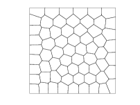
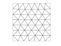
Case 1: We first consider the convergence with respect to different mesh shapes. To do so, we choose three different sequences of meshes, labeled by 1subscript1\mathcal{M}_{1}, 2subscript2\mathcal{M}_{2}, 3subscript3\mathcal{M}_{3}, as shown in Fig. 2, where 1subscript1\mathcal{M}_{1} is a sequence of meshes composed of unstructured triangles, 2subscript2\mathcal{M}_{2} is a sequence of meshes composed of distorted squares, and 3subscript3\mathcal{M}_{3} is a sequence of meshes composed of Voronoi polygons. The distorted meshes are obtained by mapping the position (ξ,ζ)𝜉𝜁(\xi,\,\zeta) of equal squares meshes through the smooth coordinate transformation

x1=ξ+110sin(2πξ)sin(2πζ),x2=ζ+110sin(2πξ)sin(2πζ).formulae-sequencesubscript𝑥1𝜉1102𝜋𝜉2𝜋𝜁subscript𝑥2𝜁1102𝜋𝜉2𝜋𝜁\displaystyle x_{1}=\xi+\frac{1}{10}\sin{(2\pi\xi)}\sin{(2\pi\zeta)},\quad x_{2}=\zeta+\frac{1}{10}\sin{(2\pi\xi)}\sin{(2\pi\zeta)}.

And the polygonal meshes are generated by the MATLAB toolbox - PolyMesher introduced in [36].

Let μ=1𝜇1\mu=1 and λ=106𝜆superscript106\lambda=10^{6}. We display the nodal values of the elliptic projection Π1𝒖hsubscriptΠ1subscript𝒖\Pi_{1}\boldsymbol{u}_{h} on 3subscript3\mathcal{M}_{3} in Fig. 3, from which we observe that the numerical solutions are well matched with the exact ones.

Refer to caption
Fig. 3: Numerical and exact solutions for λ=106𝜆superscript106\lambda=10^{6} on a polygonal mesh of 3subscript3\mathcal{M}_{3} in Test 1. (left: Mesh512, middle: numerical solution, right: exact solution)

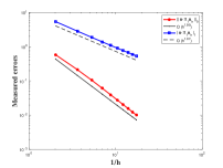
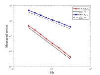
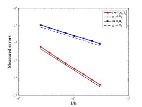
The H1superscript𝐻1H^{1} and L2superscript𝐿2L^{2} errors computed as functions of mesh size hh for the mesh sequences {i}i=13superscriptsubscriptsubscript𝑖𝑖13\{\mathcal{M}_{i}\}_{i=1}^{3} are depicted in Fig. 4 as a log-log plot. For each fixed pair (λ,μ)𝜆𝜇(\lambda,\mu), the convergence rate with respect to hh is estimated by assuming Err(h)=chαErr𝑐superscript𝛼{\rm Err}(h)=ch^{\alpha} and computing a least squares fit to this log-linear relation. We see that the errors ErrH1 and ErrL2 converge at the optimal rate 𝒪(h1)𝒪superscript1\mathcal{O}(h^{1}) and 𝒪(h2)𝒪superscript2\mathcal{O}(h^{2}) respectively, and are not affected by the shape of the mesh discretization. It is worth noting that, the proposed VEM shows a satisfactory stability with respect to the nearly incompressible case (λ=106𝜆superscript106\lambda=10^{6}).

Refer to caption
(a) Unstructued triangles
Refer to caption
(b) Distorted squares
Refer to caption
(c) Voronoi polygons
Fig. 4: L2superscript𝐿2L^{2} and H1superscript𝐻1H^{1} errors for λ=106𝜆superscript106\lambda=10^{6} on three different sequences of meshes in Test 1.

Case 2: We next investigate the locking-free property of the proposed VEM, i.e., the robustness with respect to the choice of λ𝜆\lambda. In this case, we only focus on considering the Voronoi polygonal meshes 3subscript3\mathcal{M}_{3}.

Let μ=1𝜇1\mu=1 and λ{1, 104, 107}𝜆1superscript104superscript107\lambda\in\{1,\,10^{4},\,10^{7}\}. The convergence graphs of the errors ErrH1 and ErrL2 for different values of λ𝜆\lambda are displayed in Fig. 5, and the corresponding errors ErrH1 and ErrL2 are shown in Tab. 1. We observe that all the errors are almost the same and the method converges with the optimal rates, which is in well agreement with the theoretical predictions in Theorems 4.1 and 4.2.

Tab. 1: H1superscript𝐻1H^{1} and L2superscript𝐿2L^{2} errors for λ{1, 104, 107}𝜆1superscript104superscript107\lambda\in\{1,\,10^{4},\,10^{7}\} on polygonal meshes 3subscript3\mathcal{M}_{3} in Test 1.
Mesh Choices of λ𝜆\lambda λ=1𝜆1\lambda=1 λ=104𝜆superscript104\lambda=10^{4} λ=107𝜆superscript107\lambda=10^{7}
h ##\#DOFs ErrH1 ErrL2 ErrH1 ErrL2 ErrH1 ErrL2
0.396819 166 4.859e+0 4.708e-1 4.833e+0 4.722e-1 4.833e+0 4.722e-1
0.272025 326 3.345e+0 2.494e-1 3.331e+0 2.515e-1 3.331e+0 2.515e-1
0.193715 646 2.352e+0 1.302e-1 2.337e+0 1.302e-1 2.337e+0 1.302e-1
0.140331 1278 1.635e+0 6.699e-2 1.628e+0 6.748e-2 1.628e+0 6.748e-2
0.096262 2530 1.155e+0 3.353e-2 1.147e+0 3.357e-2 1.147e+0 3.357e-2
0.065690 5066 8.148e-1 1.742e-2 8.092e-1 1.743e-2 8.092e-1 1.743e-2
0.046554 10186 5.719e-1 8.468e-3 5.690e-1 8.473e-3 5.690e-1 8.473e-3
0.033120 20326 4.047e-1 4.306e-3 4.025e-1 4.300e-3 4.025e-1 4.300e-3
Refer to caption
(a) λ=1𝜆1\lambda=1
Refer to caption
(b) λ=104𝜆superscript104\lambda=10^{4}
Refer to caption
(c) λ=107𝜆superscript107\lambda=10^{7}
Fig. 5: L2superscript𝐿2L^{2} and H1superscript𝐻1H^{1} errors for λ{1, 104, 107}𝜆1superscript104superscript107\lambda\in\{1,\,10^{4},\,10^{7}\} on polygonal meshes 3subscript3\mathcal{M}_{3} in Test 1.

Furthermore, we take λ{10j,j=0,1,,7}\lambda\in\{10^{j},j=0,1,\cdots,7\} on a fixed mesh in 3subscript3\mathcal{M}_{3} with h=0.06568980.0656898h=0.0656898. As shown in Tab. 2, the errors ErrH1 and ErrL2 are insensitive to the choice of λ𝜆\lambda, thus the proposed VEM is robust with respect to λ𝜆\lambda, i.e., it is volume locking-free.

Tab. 2: H1superscript𝐻1H^{1} and L2superscript𝐿2L^{2} errors for different values of λ𝜆\lambda on one fixed mesh of 3subscript3\mathcal{M}_{3} in Test 1.
ErrorsλErrors𝜆{\rm Errors}\setminus\lambda 111 101010 102superscript10210^{2} 103superscript10310^{3} 104superscript10410^{4} 105superscript10510^{5} 106superscript10610^{6} 107superscript10710^{7}
ErrH1 8.148e-1 8.096e-1 8.092e-1 8.092e-1 8.092e-1 8.092e-1 8.092e-1 8.092e-1
ErrL2 1.742e-2 1.741e-2 1.743e-2 1.743e-2 1.743e-2 1.743e-2 1.743e-2 1.743e-2

6.3 The mixed boundary conditions

Test 2: We solve the following linear elasticity problem on Ω=(0,1)2Ωsuperscript012\Omega=(0,1)^{2} with general boundary conditions:

{𝐝𝐢𝐯𝝈(𝒖)=𝒇inΩ,𝒖=𝒈1onΓ1.𝝈(𝒖)𝒏=𝒈2onΓ2,cases𝐝𝐢𝐯𝝈𝒖𝒇inΩ𝒖subscript𝒈1onsubscriptΓ1𝝈𝒖𝒏subscript𝒈2onsubscriptΓ2\begin{cases}-{\mathbf{div}}~{}\boldsymbol{\sigma}(\boldsymbol{u})=\boldsymbol{f}&\text{in}~{}~{}\Omega,\\ \boldsymbol{u}=\boldsymbol{g}_{1}&\text{on}~{}~{}\Gamma_{1}.\\ \boldsymbol{\sigma}(\boldsymbol{u})\boldsymbol{n}=\boldsymbol{g}_{2}&\text{on}~{}~{}\Gamma_{2},\end{cases} (6.2)

where, Γ2={(x1,x2)|0x11,x2=0}subscriptΓ2conditional-setsubscript𝑥1subscript𝑥2formulae-sequence0subscript𝑥11subscript𝑥20\Gamma_{2}=\big{\{}(x_{1},\,x_{2})~{}|~{}0\leq{x}_{1}\leq 1,x_{2}=0\big{\}} and Γ1=Ω\Γ2subscriptΓ1\ΩsubscriptΓ2\Gamma_{1}=\partial\Omega\backslash\Gamma_{2}. We select the load term 𝒇𝒇\boldsymbol{f} and the boundary conditions such that the analytical solution of problem (6.2) (cf. [38]) is

𝒖(x1,x2)=(sin(x1)sin(x2)cos(x1)cos(x2))+1λ(x1x2).𝒖subscript𝑥1subscript𝑥2matrixsubscript𝑥1subscript𝑥2subscript𝑥1subscript𝑥21𝜆matrixsubscript𝑥1subscript𝑥2\displaystyle\boldsymbol{u}(x_{1},\,x_{2})=\begin{pmatrix}\sin{(x_{1})}\sin{(x_{2})}\\ \cos{(x_{1})}\cos{(x_{2})}\end{pmatrix}+\frac{1}{\lambda}\begin{pmatrix}x_{1}\\ x_{2}\end{pmatrix}.

Here the first term is divergence-free, but the second term provides a constant divergence (2/λ)2𝜆(2/\lambda). It is clear that div𝒖=0div𝒖0{\rm div~{}}\boldsymbol{u}=0 as λ𝜆\lambda tends to infinity.

We take μ=0.5𝜇0.5\mu=0.5 and λ{1, 104, 107,1010}𝜆1superscript104superscript107superscript1010\lambda\in\{1,\,10^{4},\,10^{7},10^{10}\} on Voronoi polygonal meshes 3subscript3\mathcal{M}_{3}. The nodal values of the elliptic projection Π1𝒖hsubscriptΠ1subscript𝒖\Pi_{1}\boldsymbol{u}_{h} for λ=1010𝜆superscript1010\lambda=10^{10} are shown in Fig. 6. The results and convergence graph of the two errors ErrH1 and ErrL2 versus the mesh size hh for different choice of λ𝜆\lambda are illustrated in Tabs. 3-4 and Fig. 7, respectively. As observed, the optimal rates of convergence are achieved for both cases.

Refer to caption
Fig. 6: Numerical and exact solutions for λ=1010𝜆superscript1010\lambda=10^{10} on a polygonal mesh of 3subscript3\mathcal{M}_{3} in Test 2. (left: Mesh512, middle: numerical solution, right: exact solution)
Tab. 3: Convergence rate w.r.t. H1superscript𝐻1H^{1} norm for λ{1, 104, 107,1010}𝜆1superscript104superscript107superscript1010\lambda\in\{1,\,10^{4},\,10^{7},10^{10}\} on meshes 3subscript3\mathcal{M}_{3} in Test 2.
λh𝜆\lambda\setminus{h} 0.396819 0.275890 0.193715 0.140331 0.096262 0.065690 0.046554 0.033120 Rate
111 1.076e-1 7.381e-2 5.238e-2 3.727e-2 2.605e-2 1.847e-2 1.297e-2 9.158e-3 0.99
104superscript10410^{4} 1.079e-1 7.386e-2 5.235e-2 3.726e-2 2.604e-2 1.846e-2 1.297e-2 9.155e-3 0.99
107superscript10710^{7} 1.079e-1 7.386e-2 5.235e-2 3.726e-2 2.604e-2 1.846e-2 1.297e-2 9.155e-3 0.99
1010superscript101010^{10} 1.079e-1 7.386e-2 5.235e-2 3.726e-2 2.604e-2 1.846e-2 1.297e-2 9.155e-3 0.99
Tab. 4: Convergence rate w.r.t. L2superscript𝐿2L^{2} norm for λ{1, 104, 107,1010}𝜆1superscript104superscript107superscript1010\lambda\in\{1,\,10^{4},\,10^{7},10^{10}\} on meshes 3subscript3\mathcal{M}_{3} in Test 2.
λh𝜆\lambda\setminus{h} 0.396819 0.275890 0.193715 0.140331 0.096262 0.065690 0.046554 0.033120 Rate
111 6.188e-3 2.739e-3 1.311e-3 6.473e-4 3.094e-4 1.518e-4 7.392e-5 3.681e-5 2.05
104superscript10410^{4} 6.113e-3 2.759e-3 1.350e-3 6.775e-4 3.305e-4 1.617e-4 8.005e-5 4.015e-5 2.01
107superscript10710^{7} 6.113e-3 2.759e-3 1.350e-3 6.775e-4 3.305e-4 1.617e-4 8.005e-5 4.015e-5 2.01
1010superscript101010^{10} 6.113e-3 2.759e-3 1.350e-3 6.775e-4 3.305e-4 1.618e-4 8.015e-5 4.021e-5 2.01
Refer to caption
(a) λ=1𝜆1\lambda=1
Refer to caption
(b) λ=104𝜆superscript104\lambda=10^{4}
Refer to caption
(c) λ=107𝜆superscript107\lambda=10^{7}
Refer to caption
(d) λ=1010𝜆superscript1010\lambda=10^{10}
Fig. 7: L2superscript𝐿2L^{2} and H1superscript𝐻1H^{1} errors for λ{1, 104, 107,1010}𝜆1superscript104superscript107superscript1010\lambda\in\{1,\,10^{4},\,10^{7},10^{10}\} on polygonal meshes 3subscript3\mathcal{M}_{3} in Test 2.

6.4 The completely incompressible limiting problem

Test 3: Finally, we consider the completely incompressible problem with the exact solution given by

𝒖(x1,x2)=(sin3(πx1)sin(2πx2)sin(πx2)sin(2πx1)sin(πx1)sin3(πx2)).𝒖subscript𝑥1subscript𝑥2matrixsuperscript3𝜋subscript𝑥12𝜋subscript𝑥2𝜋subscript𝑥22𝜋subscript𝑥1𝜋subscript𝑥1superscript3𝜋subscript𝑥2\displaystyle\boldsymbol{u}(x_{1},\,x_{2})=\begin{pmatrix}-{\sin}^{3}{(\pi{x_{1}})}{\sin}{(2\pi{x_{2}})}{\sin}{(\pi{x_{2}})}\\ {\sin}{(2\pi{x_{1}})}{\sin}{(\pi{x_{1}})}{\sin}^{3}{(\pi{x_{2}})}\end{pmatrix}.

It’s easy to check that div𝒖=0div𝒖0{\rm div}~{}\boldsymbol{u}=0 and 𝒇𝒇\boldsymbol{f} is independent of λ𝜆\lambda. Now we investigate the impact of Lamé constant λ𝜆\lambda on two different sequences of meshes composed by Voronoi and distortion polygons, respectively. Let μ=1𝜇1\mu=1 and λ=1010𝜆superscript1010\lambda=10^{10}.

Refer to caption
Fig. 8: Numerical and exact solutions for λ=1010𝜆superscript1010\lambda=10^{10} on a distortion polygonal mesh in Test 3. (left: Mesh512, middle: numerical solution, right: exact solution)

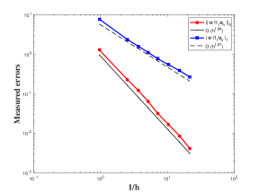
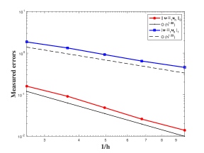
The numerical solutions are well matched with the exact ones even on distortion polygonal meshes as observed in Fig. 8. From the convergence graphs of the errors ErrH1 and ErrL2 for λ=1010𝜆superscript1010\lambda=10^{10} on two families of polygonal meshes displayed in Fig. 9, we still obtain a satisfactory result that the optimal rates of convergence are achieved for both subdivisions in the completely incompressible limiting case.
Refer to caption
(a) Voronoi polygons
Refer to caption
(b) Distortion polygons
Fig. 9: L2superscript𝐿2L^{2} and H1superscript𝐻1H^{1} errors for λ=1010𝜆superscript1010\lambda=10^{10} on Voronoi and distortion polygonal meshes in Test 3.

7 Conclusions

We propose a novel locking-free conforming VEM in the lowest order case for solving linear elasticity problems. The key is to view the mesh K𝐾K as K~~𝐾\widetilde{K} which is formed by including an interior point of each edge as an additional vertex. Then the method in [11] can be extended to the case of k=1𝑘1k=1, if V1(K)subscript𝑉1𝐾V_{1}(K) is replaced by V1(K~)subscript𝑉1~𝐾V_{1}(\widetilde{K}). The parameter-free property and the optimal error estimate are established. Numerical results are consistent with theoretical findings.

References

References

  • [1] D. Adak and S. Natarajan. Virtual element method for semilinear sine-Gordon equation over polygonal mesh using product approximation technique. Math. Comput. Simulation, 172:224–243, 2020.
  • [2] R. A. Adams. Sobolev Spaces. Academic Press, New York, 1975.
  • [3] B. Ahmad, A. Alsaedi, F. Brezzi, L. D. Marini, and A. Russo. Equivalent projectors for virtual element methods. Comput. Math. Appl., 66(3):376–391, 2013.
  • [4] E. Artioli, S. de Miranda, C. Lovadina, and L. Patruno. A stress/displacement virtual element method for plane elasticity problems. Comput. Methods Appl. Mech. Engrg., 325:155–174, 2017.
  • [5] E. Artioli, S. de Miranda, C. Lovadina, and L. Patruno. A family of virtual element methods for plane elasticity problems based on the Hellinger-Reissner principle. Comput. Methods Appl. Mech. Engrg., 340:978–999, 2018.
  • [6] E. Artioli, S. de Miranda, C. Lovadina, and L. Patruno. A dual hybrid virtual element method for plane elasticity problems. ESAIM Math. Model. Numer. Anal., 54(5):1725–1750, 2020.
  • [7] I. Babuška and M. Suri. Locking effects in the finite element approximation of elasticity problems. Numer. Math., 62(4):439–463, 1992.
  • [8] I. Babuška and M. Suri. On locking and robustness in the finite element method. SIAM J. Numer. Anal., 29(5):1261–1293, 1992.
  • [9] I. Babuška and B. Szabo. On the rates of convergence of the finite element method. Internat. J. Numer. Methods Engrg., 18(3):323–341, 1982.
  • [10] L. Beirão da Veiga, F. Brezzi, A. Cangiani, G. Manzini, L. D. Marini, and A. Russo. Basic principles of virtual element methods. Math. Models Meth. Appl. Sci., 23(1):199–214, 2013.
  • [11] L. Beirão da Veiga, F. Brezzi, and L. D. Marini. Virtual elements for linear elasticity problems. SIAM J. Numer. Anal., 51(2):794–812, 2013.
  • [12] L. Beirão da Veiga, F. Brezzi, L. D. Marini, and A. Russo. The hitchhiker’s guide to the virtual element method. Math. Models Meth. Appl. Sci., 24(8):1541–1573, 2014.
  • [13] L. Beirão da Veiga, C. Lovadina, and A. Russo. Stability analysis for the virtual element method. Math. Models Methods Appl. Sci., 27(13):2557–2594, 2017.
  • [14] K. Berbatov, B. S. Lazarov, and A. P. Jivkov. A guide to the finite and virtual element methods for elasticity. Appl. Numer. Math., 169:351–395, 2021.
  • [15] C. Bernardi and G. Raugel. Analysis of some finite elements for the Stokes problem. Math. Comp., 44(169):71–79, 1985.
  • [16] D. Boffi, F. Brezzi, and M. Fortin. Mixed finite element methods and applications, volume 44 of Springer Series in Computational Mathematics. Springer, Heidelberg, 2013.
  • [17] S. C. Brenner and L. R. Scott. The Mathematical Theory of Finite Element Methods. Springer, New York, 3rd edition, 2008.
  • [18] S. C. Brenner and L. Sung. Linear finite element methods for planar linear elasticity. Math. Comp., 59(200):321–338, 1992.
  • [19] E. Cáceres, G. N. Gatica, and F. A. Sequeira. A mixed virtual element method for a pseudostress-based formulation of linear elasticity. Appl. Numer. Math., 135:423–442, 2019.
  • [20] C. Carstensen and M. Schedensack. Medius analysis and comparison results for first-order finite element methods in linear elasticity. IMA J. Numer. Anal., 35(4):1591–1621, 2015.
  • [21] L. Chen and J. Huang. Some error analysis on virtual element methods. Calcolo, 55(1):Paper No. 5, 23, 2018.
  • [22] L. Chen and X. Huang. Nonconforming virtual element method for 2m2𝑚2m-th order partial differential equations in Rnsuperscript𝑅𝑛R^{n}. Math. Comput., 89(324):1711–1744, 2020.
  • [23] M. Costabel and M. Dauge. On the inequalities of Babuška-Aziz, Friedrichs and Horgan-Payne. Arch. Ration. Mech. Anal., 217(3):873–898, 2015.
  • [24] F. Dassi, C. Lovadina, and M. Visinoni. A three-dimensional Hellinger-Reissner virtual element method for linear elasticity problems. Comput. Methods Appl. Mech. Engrg., 364:112910, 17, 2020.
  • [25] F. Dassi and G. Vacca. Bricks for the mixed high-order virtual element method: projectors and differential operators. Appl. Numer. Math., 155:140–159, 2020.
  • [26] V. Dhanush and S. Natarajan. Implementation of the virtual element method for coupled thermo-elasticity in Abaqus. Numer. Algorithms, 80(3):1037–1058, 2019.
  • [27] A. L. Gain, C. Talischi, and G. H. Paulino. On the virtual element method for three-dimensional linear elasticity problems on arbitrary polyhedral meshes. Comput. Methods Appl. Mech. Engrg., 282:132–160, 2014.
  • [28] Y. Guo and J. Huang. A robust finite element method for elastic vibration problems. Comput. Methods Appl. Math., 20(3):481–500, 2020.
  • [29] G. Harper, R. Wang, J. Liu, S. Tavener, and R. Zhang. A locking-free solver for linear elasticity on quadrilateral and hexahedral meshes based on enrichment of Lagrangian elements. Comput. Math. Appl., 80(6):1578–1595, 2020.
  • [30] J. Huang and S. Lin. A posteriori error analysis of a non-consistent virtual element method for reaction diffusion equations. Appl. Math. Lett., 122:Paper No. 107531, 10, 2021.
  • [31] X. Huang. Nonconforming virtual element method for 2m𝑚mth order partial differential equations in nsuperscript𝑛\mathbb{R}^{n} with m>n𝑚𝑛m>n. Calcolo, 57(4):42, 2020.
  • [32] X. Huang and J. Huang. The compact discontinuous Galerkin method for nearly incompressible linear elasticity. J. Sci. Comput., 56(2):291–318, 2013.
  • [33] D. Y. Kwak and H. Park. Lowest-order virtual element methods for linear elasticity problems. Comput. Methods Appl. Mech. Engrg., 390:Paper No. 114448, 2022.
  • [34] D. Mora and G. Rivera. A priori and a posteriori error estimates for a virtual element spectral analysis for the elasticity equations. IMA J. Numer. Anal., 40(1):322–357, 2020.
  • [35] B. D. Reddy and D. van Huyssteen. A virtual element method for transversely isotropic elasticity. Comput. Mech., 64(4):971–988, 2019.
  • [36] C. Talischi, G. H. Paulino, A. Pereira, and I. F. M. Menezes. Polymesher: a general-purpose mesh generator for polygonal elements written in Matlab. Struct. Multidiscip. Optim., 45(3):309–328, 2012.
  • [37] X. Tang, Z. Liu, B. Zhang, and M. Feng. A low-order locking-free virtual element for linear elasticity problems. Comput. Math. Appl., 80(5):1260–1274, 2020.
  • [38] C. Wang, J. Wang, R. Wang, and R. Zhang. A locking-free weak Galerkin finite element method for elasticity problems in the primal formulation. J. Comput. Appl. Math., 307:346–366, 2016.
  • [39] B. Zhang and M. Feng. Virtual element method for two-dimensional linear elasticity problem in mixed weakly symmetric formulation. Appl. Math. Comput., 328:1–25, 2018.
  • [40] B. Zhang, J. Zhao, Y. Yang, and S. Chen. The nonconforming virtual element method for elasticity problems. J. Comput. Phys., 378:394–410, 2019.
  • [41] Z. Zhang. Analysis of some quadrilateral nonconforming elements for incompressible elasticity. SIAM J. Numer. Anal., 34(2):640–663, 1997.