Tracking Most Significant Arm Switches in Bandits

Abstract

In bandit with distribution shifts, one aims to automatically adapt to unknown changes in reward distribution, and restart exploration when necessary. While this problem has been studied for many years, a recent breakthrough of Auer et al. (2018, 2019) provides the first adaptive procedure to guarantee an optimal (dynamic) regret $\sqrt{LT}$, for $T$ rounds, and an unknown number $L$ of changes. However, while this rate is tight in the worst case, it remained open whether faster rates are possible, without prior knowledge, if few changes in distribution are actually severe.

To resolve this question, we propose a new notion of significant shift, which only counts very severe changes that clearly necessitate a restart: roughly, these are changes involving not only best arm switches, but also involving large aggregate differences in reward overtime. Thus, our resulting procedure adaptively achieves rates always faster (sometimes significantly) than $O(\sqrt{ST})$, where $S\ll L$ only counts best arm switches, while at the same time, always faster than the optimal $O(V^{\frac{1}{3}}T^{\frac{2}{3}})$ when expressed in terms of total variation $V$ (which aggregates differences overtime). Our results are expressed in enough generality to also capture non-stochastic adversarial settings.

1 Introduction

In Multi-armed bandit (MAB) an agent sequentially chooses an action, out of a finite set of $K$ actions (or arms), based on partial and uncertain feedback in the form of rewards $Y_{t}(a)$ for past actions $a\in[K]$ (a pull of arm $a$) (see Bubeck and Cesa-Bianchi, 2012; Slivkins, 2019; Lattimore and Szepesvári, 2020, for surveys). The goal is to maximize the cumulative reward.

We consider the setting of switching bandits, where the distributions of arms’ rewards change an unknown number of times, say $L$ times, till a time horizon $T$. Performance is then measured by a dynamic regret which compares rewards against those of the best arm at each round $t$ (i.e., the arm maximizing mean rewards $\mu_{t}(a)\doteq\mathbb{E}\ Y_{t}(a)$ over $a\in[K]$). Garivier and Moulines (2011) showed that existing procedures (Auer et al., 2002; Kocsis and Szepesvári, 2006) could achieve a dynamic regret $\tilde{O}(\sqrt{LT})$, however, requiring knowledge of $L$. This requirement on knowledge of $L$, although impractical, remained standing till a recent breakthrough of Auer et al. (2018, 2019), with important follow-ups in Chen et al. (2019); Wei and Luo (2021) for contextual settings. Soon afterwards, other parameter-free approaches were studied in Besson et al. (2022); Mukherjee and Maillard (2019). This work is concerned with the achievability of faster rates that better account for mild to severe changes.

In particular, the $\sqrt{LT}$ rate is understood to be tight only in the worst-case, since $L$ counts all changes in distribution, even mild ones. This is evidenced, e.g., by alternative bounds of the form $V^{\frac{1}{3}}T^{\frac{2}{3}}$ (see e.g. Chen et al., 2019), when the total variation $V\doteq\sum_{t}\max_{a}\left|\mu_{t+1}(a)-\mu_{t}(a)\right|$ (aggregating differences) is small, e.g., $V\lesssim 1/\sqrt{T}$, yielding regret $\sqrt{T}$, irrespective of the $L$ changes. However, the total variation perspective can also be pessimistic as $V$ could be large, up to $O(T)$ (yielding regret $O(T)$), even when the best arm remains fixed across the $L$ changes.

Outside of best arm switches, a dynamic regret of $\sqrt{T}$ remains possible (Allesiardo et al., 2017), irrespective of $V$ and $L$. In light of this, achieving faster rates of $\sqrt{ST}$, for an unknown number $S\ll L$ of best arm switches, is understood as a key open problem (Auer et al., 2019; Foster et al., 2020).

We in fact aim beyond solving this problem, as even the quantity $S$ overcounts the severity of changes, e.g., when $V$ remains small across best arm switches. Instead we propose a new notion of significant shift which aims to only count severe changes in mean reward that clearly necessitate a restart. Integral to our definition is the idea that a restart (in exploration) is only necessary when there are no safe arms left to play. Here, an arm $a$ is considered safe if its total regret over any interval $[s_{1},s_{2}]$ within a phase, namely $\sum_{t=s_{1}}^{s_{2}}\max_{a^{\prime}}\mu_{t}(a^{\prime})-\mu_{t}(a)$, is $o(\sqrt{s_{2}-s_{1}})$.

As such, a significant phase ends only when no safe arm remains, which in particular does not count best arm switches that do not last long enough to hurt regret. For example, a change from arm $a$ to $a^{\prime}$ as a new best arm, with a large gap $\mu_{t}(a^{\prime})-\mu_{t}(a)=\delta$, constant over the next rounds, is ignored if another switch within the next $O(\delta^{-2})$ rounds, reverts back to $a$ as the best arm. Also, unlike with total variation, aggregate differences are ignored outside of best arm switches.

As a simple sanity check that other distributional changes beyond significant shifts are safely ignored, we show in Proposition 1 that a simple oracle that effectively ignores all other changes, achieves regret $\sqrt{\left|I\right|}$ over any significant phase $I$ of length $\left|I\right|$. Furthermore, such a basic guarantee of $\sum_{I}\sqrt{\left|I\right|}$ total regret over significant phases $I$, immediately implies (1) a rate of $\sqrt{{\tilde{L}}T}$ where ${\tilde{L}}\leq S\leq L$ only counts significant shifts, and (2) a rate of $V^{\frac{1}{3}}T^{\frac{2}{3}}$ in terms of total variation.

Finally we show that these guarantees are attained adaptively, i.e., with no prior knowledge of the environment (Theorem 1). Our key algorithmic innovation over previous works is that, rather than aiming to detect changes in the mean rewards $\mu_{t}(a)$ of arms $a$, we focus on detecting changes in the aggregate gaps in mean rewards between arms, i.e., in $\sum_{t}\mu_{t}(a^{\prime})-\mu_{t}(a)$, a stable quantity across milder shifts. While this quantity does not directly track the dynamic regret of arm $a$ (as the comparator $a^{\prime}$ here is independent of $t$), it will turn out sufficient (see beginning of Section 4). Now, this quantity is estimable via a simple unbiased (importance-weighted) statistic, which concentrates via martingale inequalities and can thus be used for change-point detection; however, the estimate does require replays of previously discarded arms $a^{\prime}$. These replays are carefully scheduled so as to not overly affect regret, as inspired by previous work (e.g. Auer et al., 2019; Chen et al., 2019). The resulting procedure META is described in Algorithm 4.

Our results not only concern the stochastic switching bandits setting, but extend to the adversarial setting, since we allow for shifts at every round, though they may not trigger significant shifts, and as well as allow for deterministic rewards (i.e., degenerate distributions). Formally, our setting admits a randomized, oblivious adversary which decides, a priori, an arbitrary sequence of distributions for the rewards (Slivkins, 2019).

Finally, we remark that a recent paper of Abbasi-Yadkori et al. (2022) independently and concurrently also resolves the problem of obtaining the $\sqrt{ST}$ rate adaptively.

1.1 Further Discussion on Related Work

The work of Manegueu et al. (2021) is closest in spirit to this paper, also establishing dynamic regret bounds scaling with a generalized notion of shifts. However, their notion is considerably weaker, as it for instance counts changes resulting in large differences $|\mu_{t}(a)-\mu_{t-1}(a)|$ in mean rewards of a best arm $a$, even when the best arm does not change. More importantly, their procedures are non-adaptive, requiring knowledge of the number of such changes.

Many works have considered the problem of achieving regret depending only on the number of best arm switches $S$, which we discuss next.

First, in the setting of adversarial bandits with deterministic rewards, the EXP3.S procedure of (Auer et al., 2002; Auer, 2002) can achieve a near-optimal dynamic regret bound $\tilde{O}(\sqrt{ST})$, but requiring knowledge of $S$. However, for more practical situations where $S$ is unknown, the best regret guarantee to our knowledge is $O(\sqrt{ST}+T^{3/4})$, obtained by combining the Bandits-over-Bandits strategy of Cheung et al. (2019) with EXP3.S (Foster et al., 2020; Auer et al., 2019). It is also known that EXP3.S alone can obtain the suboptimal rate of $\tilde{O}(S\sqrt{T})$ for unknown $S$ by setting the parameters of the algorithm independently of $S$ (Auer, 2002).

The more general problem of obtaining adaptive switching regret $\sqrt{ST}$ for all $S$ remains open and is beyond the scope of this paper (Foster et al., 2020). Relatedly, recent work of Marinov and Zimmert (2021) showed the impossibility of obtaining such adaptive switching regret bounds against an adaptive adversary (where switch points may depend on the algorithm’s actions).

Second, the work of Allesiardo et al. (2017) studies dynamic regret in the same randomized adversarial bandit setting as this paper (which as stated above also recovers the deterministic setting). They provide two algorithms that get regret $S\sqrt{T}$ and $T^{2/3}\sqrt{S}$, which do not match the optimal regret of $\sqrt{ST}$. Furthermore, their procedures either require knowledge of $S$ or lower-bounds on the magnitude of the changes to allow for easier detection.

In contrast to the above works, we impose no requirements on detectability, nor knowledge of the environment, while achieving rates (at times considerably) faster than $\sqrt{ST}$.

A different body of literature considers more structured changes in reward distributions. In rested rotting bandits, the reward of an arm decreases depending on its amount of play (Seznec et al., 2020; Levine et al., 2017; Heidari et al., 2016; Seznec et al., 2019). Slivkins and Upfal (2008) study a setting where the rewards follow a Brownian motion across time. Several works also studied a subcase of the above mentioned drifting environment: slowly varying bandits, parametrized by a local limit on the change of rewards between consecutive rounds (Wei and Srivatsva, 2018; Krishnamurthy and Gopalan, 2021). Generally, such stronger structural conditions can yield faster rates at times, often of the form $\phi\cdot\log(T)$, for some problem dependent quantity $\phi$.

Finally, various works combine adversarial and stochastic approaches to simultaneously address both settings (Bubeck and Slivkins, 2012; Seldin and Slivkins, 2014; Auer and Chiang, 2016). However, these approaches measure regret to the best arm in hindsight, whereas our results hold for the stronger dynamic regret.

2 Problem Setting

In our environment, an oblivious adversary decides a sequence of distributions on the rewards. This subsumes the stochastic switching bandit problem and is also a generalization of the adversarial bandit problem with deterministic rewards since our reward distributions can have zero variance.

We assume a decision space $[K]$ of $K$ arms with bounded reward distributions: arm $a$ at round $t$ has reward $Y_{t}(a)\in[0,1]$ with mean $\mu_{t}(a)$. A (possibly randomized) policy $\pi$ selects at each round $t$ some arm $\pi_{t}\in[K]$ and observes reward $Y_{t}(\pi_{t})$. The goal is to minimize the dynamic regret, i.e., the expected regret to the best arm at each round. This is defined as:

$$R(\pi,T)\doteq\sum_{t=1}^{T}\max_{a\in[K]}\mu_{t}(a)-\mathbb{E}\left[\sum_{t=1}^{T}\mu_{t}(\pi_{t})\right].$$

In this paper, we rely heavily on analyzing the gaps in mean rewards between arms. Therefore, for convenience, let $\delta_{t}(a^{\prime},a)\doteq\mu_{t}(a^{\prime})-\mu_{t}(a)$ denote the relative gap of arms $a$ to $a^{\prime}$ at round $t$. Define the worst gap of arm $a$ as $\delta_{t}(a)\doteq\max_{a^{\prime}\in[K]}\delta_{t}(a^{\prime},a)$, corresponding to the instantaneous regret of playing $a$ at round $t$. Notice that the above regret is then given as $\sum_{t\in[T]}\mathbb{E}[\delta_{t}(\pi_{t})]$.

Significant Shifts and Phases.

First, we say arm $a$ incurs significant regret on interval $[s_{1},s_{2}]$ if:

$$\sum_{t=s_{1}}^{s_{2}}\delta_{t}(a)\geq\sqrt{K\cdot(s_{2}-s_{1})}. \star$$ ()

Intuitively, such an arm is no longer safe to play. Now, if instead ($\star$ ‣ 2) holds for no interval in a time period, the arm $a$ incurs little regret over that period. We therefore propose to record a significant shift only when there is no safe arm left to play. This idea leads to the following recursive definition.

Definition 1

Let $\tau_{0}=1$. Then, recursively for $i\geq 0$, the $(i+1)$-th significant shift is recorded at time $\tau_{i+1}$, which denotes the earliest time $\tau\in(\tau_{i},T]$ such that for every arm $a\in[K]$, there exists rounds $s_{1}<s_{2},[s_{1},s_{2}]\subseteq[\tau_{i},\tau]$, such that arm $a$ has significant regret ($\star$ ‣ 2) on $[s_{1},s_{2}]$.

We will refer to intervals $[\tau_{i},\tau_{i+1}),i\geq 0,$ as (significant) phases. The unknown number of such phases (by time $T$) is denoted ${\tilde{L}}+1$, whereby $[\tau_{\tilde{L}},\tau_{{\tilde{L}}+1})$, for $\tau_{{\tilde{L}}+1}\doteq T+1,$ denotes the last phase.

It should be clear from the above that not all shifts are counted, and in fact not all best arm switches are counted, since simply having $\delta_{t}(a)>0$, where $a$ was previously a best arm, does not trigger a significant shift. For further intuition that a procedure need only restart exploration upon a significant shift, notice that the last arm to trigger ($\star$ ‣ 2) in a phase $I$, only incurs regret $O(\sqrt{\left|I\right|})$ over the phase. As long as there exists a safe arm to play, a small regret may be achieved if all other arms are rejected in time as they become unsafe in a phase. This intuition is verified in the next proposition.

Proposition 1 (Sanity Check)

For each round $t$ belonging to phase $[\tau_{i},\tau_{i+1})$, define a good arm set $\mathcal{G}_{t}$ as the set of safe arms, i.e., arms which do not yet satisfy ($\star$ ‣ 2) on any subinterval of $[\tau_{i},t]$. Then, consider the following oracle procedure $\pi$: at each round $t$, $\pi$ plays a random arm $a\in\mathcal{G}_{t}$ with probability $1/|\mathcal{G}_{t}|$. We then have:

$$R(\pi,T)\leq\log(K)\sum_{i=0}^{\tilde{L}}\sqrt{K(\tau_{i+1}-\tau_{i})}.$$

Proof 2.1.

See Appendix A.

It is not hard to show, essentially by Jensen’s, that a rate of the form above is always faster than $O(\sqrt{{\tilde{L}}T}\land V^{\frac{1}{3}}T^{\frac{2}{3}})$. This is shown for instance in Corollaries 2 and 3.

It is therefore left to design a procedure which mimics the above oracle, i.e., that quickly detects and rejects unsafe arms, and restarts in time whenever no safe arm is left. Note that we may not be able to estimate $\sum_{t}\delta_{t}(a)$, but since there exists a relatively safe arm $a^{\prime}$ in each phase, it’ll be enough to ensure small regret w.r.t. such $a^{\prime}$. Thus, we will need only track $\sum_{t}\delta_{t}(a^{\prime},a)$.

3 Results Overview

Our main result is a dynamic regret bound of similar order to Proposition 1 without knowledge of the environment, e.g., the significant shift times, or the number of significant phases. It is stated for our algorithm META (Algorithm 4 of Section 4), which, for simplicity, requires knowledge of the time horizon $T$. Knowledge of $T$ is easily removed using a doubling trick (see Proposition 4).

Theorem 1.

Let $\pi$ denote the META procedure. Let $\{\tau_{i}\}_{i=0}^{\tilde{L}+1}$ denote the unknown significant shift times of Definition 1. We then have for some $C>0$:

$$R(\pi,T)\leq C\log^{3}(T)\sum_{i=0}^{{\tilde{L}}}\sqrt{K\cdot(\tau_{i+1}-\tau_{i})}.$$

Remark 1

The $\log$ dependence in the rate of Theorem 1 can be improved to

$$\sum_{i=0}^{{\tilde{L}}}\log(K)\log^{3/2}(KT)\sqrt{K\cdot(\tau_{i+1}-\tau_{i})}+\log(K)\log^{2}(KT)\cdot K,$$

by modifying the threshold in (2) to $\sqrt{K\log(T)\cdot(s_{2}-s_{1})\vee K^{2}\log^{2}(T)}$ and adjusting Proposition 6 in the same manner. This is avoided in the analysis to simplify presentation.

Note that, while the rates above are similar to the oracle rates on Proposition 1, META may not actually achieve regret $\sqrt{\left|I\right|}$ over each phase $I$, but only guarantees $\sum_{I}\sqrt{\left|I\right|}$ on aggregate.

The following corollary is immediate from Jensen’s inequality.

Corollary 2 (Bounding by Number of Significant Shifts).

Using the same notation of Theorem 1:

$$R(\pi,T)\leq C\log^{3}(T)\cdot\sqrt{({\tilde{L}}+1)KT}.$$

Since ${\tilde{L}}\leq S$, we have by Corollary 2 that META recovers the $\tilde{O}(\sqrt{SKT})$ rate of EXP3.S, however without knowledge of ${\tilde{L}}$ or $S$. The rate can in fact be much faster when ${\tilde{L}}\ll S$.

The $\tilde{O}(\sqrt{{\tilde{L}}KT})$ rate is optimal up to $\log$ terms in the worst-case since any algorithm which has to solve ${\tilde{L}}$ independent adversarial bandit problems of length $T/{\tilde{L}}$ can be forced to suffer regret $\Omega(\sqrt{KT/{\tilde{L}}})$ on each phase, following similar arguments as in Auer (2002); Auer et al. (2019).

The next corollary asserts that Theorem 1 also recovers the optimal rate for the drifting environment setting, i.e., in terms of total-variation $V$. The proof (Appendix C) follows from the definition of significant shift (Definition 1) in that the total-variation over every phase $[\tau_{i},\tau_{i+1})$ can be bounded below by roughly $1/\sqrt{\tau_{i+1}-\tau_{i}}$.

Corollary 3 (Bounding by Total Variation).

Let $V\doteq\sum_{t=2}^{T}\max_{a\in[K]}|\mu_{t}(a)-\mu_{t-1}(a)|$ be the unknown total variation of change in the rewards. Using the same notation of Theorem 1:

$$R(\pi,T)\leq C\log^{3}(T)\left(\sqrt{KT}+(KV)^{1/3}T^{2/3}\right).$$

Finally, as stated above, a simple doubling trick removes the need to know $T$.

Proposition 4.

The doubling-horizon version of META has dynamic regret

$$\tilde{O}\!\left(\sqrt{({\tilde{L}}+1)KT}\land\left(\sqrt{KT}+(KV)^{1/3}T^{2/3})\right)\right).$$

4 Algorithm

[h] Meta-Elimination while Tracking Arms (META) Input: horizon $T$.
Initialize: round count $t\leftarrow 1$.
Episode Initialization (setting global variables $t_{\ell},\operatorname{\mathcal{A}_{\text{master}}},B_{s,m}$):
$t_{\ell}\leftarrow t$. *$t_{\ell}$ indicates start of $\ell$-th episode. $\operatorname{\mathcal{A}_{\text{master}}}\leftarrow[K]$ *Master candidate arm set. For each $m=2,4,\ldots,2^{\lceil\log(T)\rceil}$ and $s=t_{\ell}+1,\ldots,T$:
Sample and store $B_{s,m}\sim\text{Bernoulli}\left(\frac{1}{\sqrt{m\cdot(s-t_{\ell})}}\right)$. *Set replay schedule. Run ${\small\textsf{{Base-Alg}}}(t_{\ell},T+1-t_{\ell})$.
$t<T$restart from Line 2 (i.e. start a new episode).

[h]Base-Alg$(\operatorname{\it{t}_{{\text{start}}}},m_{0})$: elimination with randomized arm-pulls Input: starting round $\operatorname{\it{t}_{{\text{start}}}}$, scheduled duration $m_{0}$.
Initialize: $t\leftarrow\operatorname{\it{t}_{{\text{start}}}}$, $\mathcal{A}_{t}\leftarrow[K]$. *$t$ and $\mathcal{A}_{t}$ are global variables. $t\leq T$ Play a random arm $a\in\mathcal{A}_{t}$ selected with probability $1/|\mathcal{A}_{t}|$.
Let $\mathcal{A}_{\text{current}}\leftarrow\mathcal{A}_{t}$ *Save current candidate arm set. Increment $t\leftarrow t+1$.
$\exists m\text{{\,such that }}B_{t,m}>0$ Let $m\doteq\max\{m\in\{2,4,\ldots,2^{\lceil\log(T)\rceil}\}:B_{t,m}>0\}$. *Set maximum replay length. Run ${\small\textsf{{Base-Alg}}}(t,m)$. *Replay interrupted by child replay. $t>\operatorname{\it{t}_{{\text{start}}}}+m_{0}$ RETURN. Evict bad arms:
$\operatorname{\mathcal{A}_{\text{master}}}\leftarrow\operatorname{\mathcal{A}_{\text{master}}}\backslash\{a\in[K]:\text{$\exists$ rounds $[s_{1},s_{2}]\subseteq[t_{\ell},t)$ s.t. \eqref{eq:elim} holds}\}$.
$\mathcal{A}_{t}\leftarrow\mathcal{A}_{\text{current}}\backslash\{a\in[K]:\text{$\exists$ rounds $[s_{1},s_{2}]\subseteq[\operatorname{\it{t}_{{\text{start}}}},t)$ s.t. \eqref{eq:elim} holds}\}$.
Restart criterion: $\operatorname{\mathcal{A}_{\text{master}}}=\emptyset$RETURN.

As explained earlier in the introduction, a main departure from past work is that, in order to detect a (significant) shift, we aim to detect changes in aggregate gaps $\sum_{t=s_{1}}^{s_{2}}\delta_{t}(a^{\prime},a)$ between pairs of arms, over intervals $[s_{1},s_{2}]$, rather than, e.g., changes in mean rewards $\mu_{t}(a)$. In particular this allows us to avoid triggering a restart upon benign changes in distribution.

However, as previously discussed, $\sum_{t=s_{1}}^{s_{2}}\delta_{t}(a^{\prime},a)$ does not directly track the dynamic regret $\sum_{t=s_{1}}^{s_{2}}\max_{a^{\prime}}\delta_{t}(a^{\prime},a)$. Fortunately, for one, it is a lower bound on the dynamic regret; thus if it is large, so is the dynamic regret. On the other hand, if $\max_{a^{\prime}}\sum_{t=s_{1}}^{s_{2}}\delta_{t}(a^{\prime},a)$ remains small for some $a$ over any $[s_{1},s_{2}]$, we can rely on the very definition of significant shift to infer that $a$ remains relatively safe to play: let $a^{\prime}$ be the last arm to incur significant regret ($\star$ ‣ 2) in a phase $I$, $a$ and $a^{\prime}$ must then have similar regret $\sqrt{\left|I\right|}$ over $I$.

Now, as we eliminate arms overtime, estimating $\sum_{t=s_{1}}^{s_{2}}\delta_{t}(a^{\prime},a)$ involves replaying previously eliminated arms. This has to be done on a careful schedule so as not to overly affect regret when there is no change; here we simply borrow from similar schedules as in previous work (Auer et al., 2019; Chen et al., 2019; Wei and Luo, 2021).

We next establish some useful terminology for discussing our approach in more detail.

Terminology and Overview.

Our main procedure META operates in episodes, starting each episode by playing a base algorithm for a possible duration equal to the rounds left till $T$. Now, a base algorithm occasionally activates its own base algorithms of varying durations (Line 4 of Algorithm 4), called replays, aimed at detecting changes according to the aforementioned schedule (stored in the variable $\{B_{s,m}\}$). We refer to the base algorithm playing at round $t$ as the active base algorithm. This results in recursive calls, from parent to child instances of Base-Alg, as depicted in Figure 1.

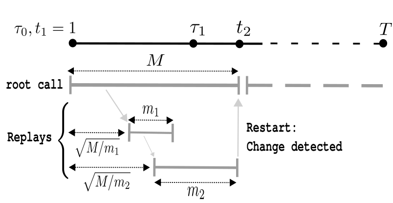
Figure 1: Shown are two replay durations $m=m_{1}\text{ or }m_{2}$, and corresponding replays are shown (gray segments) at intervals of roughly ${\sqrt{M/m}}$ rounds, where $M$ is the eventual length of an episode. Each replay (gray segments) aims to detect a $1/\sqrt{m}$ magnitude change, i.e., an average gap $\frac{1}{m}\sum_{t=1}^{m}\delta_{t}(a)$ of order $1/\sqrt{m}$. As a recursive procedure, the replays of Base-Alg  form a parent-child relationship as depicted.

Each instance of Base-Alg maintains at each round $t$ a candidate arm set $\mathcal{A}_{t}$, initialized to $[K]$ at $t=\operatorname{\it{t}_{{\text{start}}}}$ and further refined as it eliminates suboptimal arms. Instances of Base-Alg and META share information, in the form of global variables as listed below:

• All variables defined in META, namely $t_{\ell},t,\mathcal{A}_{\text{master}},\{B_{s,m}\}$ (see Lines 4–4 of Algorithm 4).

• All arms played at any round $t$, along with observed rewards $Y_{t}(a)$, and the candidate arm set $\mathcal{A}_{t}$. As such, the size of $\mathcal{A}_{t}$ can fluctuate throughout an episode as it is reset to $[K]$ by new replays, i.e., as a base algorithm is activated by a parent, and again reset as the parent resumes (as maintained via $\mathcal{A}_{\text{current}}$).

By sharing these global variables, any replay can trigger a new episode: every time an arm is evicted by a replay, it is also evicted from $\operatorname{\mathcal{A}_{\text{master}}}$, essentially the candidate arm set for the current episode. A new episode is triggered when $\operatorname{\mathcal{A}_{\text{master}}}$ is empty, i.e., there is no safe arm left to play.

Eviction Criteria and Critical Estimates.

A running intuition so far is that Base-Alg ejects any arm $a$ from $\mathcal{A}_{t}$ when it determines that $\sum_{t=s_{1}}^{s_{2}}\delta_{t}(a^{\prime},a)$ is large. Note that any rejected arm is also immediately rejected by the parent when a child terminates.

Now, the quantity $\sum_{t=s_{1}}^{s_{2}}\delta_{t}(a^{\prime},a)$ is estimated as $\sum_{t=s_{1}}^{s_{2}}\hat{\delta}_{t}(a^{\prime},a)$, whereby the relative gap $\delta_{t}(a^{\prime},a)$ is estimated by importance weighting as:

$$\hat{\delta}_{t}(a^{\prime},a)\doteq|\mathcal{A}_{t}|\cdot\left(Y_{t}(a^{\prime})\cdot\boldsymbol{1}\{\pi_{t}=a^{\prime}\}-Y_{t}(a)\cdot\boldsymbol{1}\{\pi_{t}=a\}\right).$$ (1)

Note that the above is an unbiased estimate of $\delta_{t}(a^{\prime},a)$ whenever $a^{\prime}$ and $a$ are both in $\mathcal{A}_{t}$ at time $t$. It then follows that the difference $\sum_{t=s_{1}}^{s_{2}}\left(\hat{\delta}_{t}(a^{\prime},a)-\delta_{t}(a^{\prime},a)\right)$ is a martingale that concentrates at a rate roughly $\sqrt{K(s_{2}-s_{1})}$ (see Proposition 6).

An arm $a$ is then evicted at round $t$ if, for some fixed $C_{0}>0$ , $\exists$ rounds $s_{1}<s_{2}\leq t$ such that:

$$\max_{a^{\prime}\in[K]}\sum_{t=s_{1}}^{s_{2}}\hat{\delta}_{s}(a^{\prime},a)>\log(T)\sqrt{C_{0}\cdot\left(K(s_{2}-s_{1})\vee K^{2}\right)}.$$ (2)

5 Regret Analysis

Continuing from the discussion at the beginning of Section 3, for any arm $a$ being played by META, ideally, the regret to the last arm $a^{\prime}$ to incur significant regret in any given phase remains small, lest $a$ would be evicted before such regret $\sum_{t=s_{1}}^{s_{2}}\delta_{t}(a^{\prime},a)$ is too large over a given interval $[s_{1},s_{2}]$. However, we can only reliably estimate such regret via $\sum_{t=s_{1}}^{s_{2}}\hat{\delta}_{t}(a^{\prime},a)$ when both $a,a^{\prime}$ are being played over $[s_{1},s_{2}]$ (in fact, this estimator is only unbiased when this is the case).

To this end, we will decompose each phase into bad segments where $\sum_{t=s_{1}}^{s_{2}}\delta_{t}(a^{\prime},a)$ is large (see Definition 9); we then argue that, while it is safe to miss a few such bad segments, a timely replay of Base-Alg is likely to occur over some such segment, ensuring both $a,a^{\prime}$ are being played, and thus leading to the detection that $a$ is no longer safe. Note that it is easy to argue that such a perfect replay will not evict arm $a^{\prime}$ since otherwise $\max_{a^{\prime\prime}}\sum_{t=s_{1}}^{s_{2}}\delta_{t}(a^{\prime\prime},a^{\prime})\leq\sum_{t=s_{1}}^{s_{2}}\delta_{t}(a^{\prime})$ must be large, i.e., $a^{\prime}$ must have significant regret on some interval before the end of the phase. For simplicity, we’ll refer to such well-timed replays as perfect replays. This is discussed in more detail in Section 5.4.

Preliminaries.

Throughout the proof $c_{1},c_{2},\ldots$ will denote positive constants not depending on $T$ or any distributional parameters. Recall from Line 4 of Algorithm 4 that $t_{\ell}$ is the first round of the $\ell$-th episode. WLOG, there are $T$ total episodes and, by convention, we let $t_{\ell}\doteq T+1$ if only $\ell-1$ episodes occurred by round $T$.

We first handle the simple case of $T<K$. In this case, the bound of Theorem 1 vacuously holds:

$$\sum_{i=0}^{\tilde{L}}\sqrt{K\cdot(\tau_{i+1}-\tau_{i})}\geq\sqrt{K\cdot(\tau_{{\tilde{L}}+1}-\tau_{0})}=\sqrt{K\cdot(T+1-1)}>T.$$

Thus, it remains to show Theorem 1 for $T\geq K$.

5.1 Decomposing the Total Regret

Continuing from the earlier discussion, we first decompose the total regret into (i) the regret of the last arm to incur significant regret in a phase and (ii) the relative regret of META to this last safe arm. We start by defining notation, to be used throughout, for this last safe arm,

Definition 5 (Last Safe Arm in a Phase).

As described in Section 2, there is a safe arm to play in each phase $i$, namely the last arm to incur significant regret ($\star$ ‣ 2) in phase $i$, which we denote $a_{i}^{\sharp}$. We then let $a_{t}^{\sharp}$, $t\in[0,T]$, track $a_{i}^{\sharp}$ across phases, that is $a_{t}^{\sharp}\doteq a_{i}^{\sharp}$ for $t\in[\tau_{i},\tau_{i+1})$.

Then, the total regret decomposes as:

$$\mathbb{E}\left[\sum_{t=1}^{T}\delta_{t}(\pi_{t})\right]=\sum_{t=1}^{T}\delta_{t}(a_{t}^{\sharp})+\mathbb{E}\left[\sum_{t=1}^{T}\delta_{t}(a_{t}^{\sharp},\pi_{t})\right].$$

Note that there is no randomness in the first sum of the R.H.S. above since the safe arm $a_{t}^{\sharp}$ is non-random for any fixed round $t$. This first sum is handled similarly to the guarantee for the oracle procedure of Proposition 1, as each arm $a_{i}^{\sharp}$ is safe to play in phase $i$. In particular, showing this sum is of the desired order follows from taking $\mathcal{S}_{t}=\{a_{t}^{\sharp}\}$ in Lemma A.1 of Appendix A.

So, it remains to bound the relative regret of $\pi_{t}$ to the safe arm $a_{t}^{\sharp}$. To this end, we will first show that the estimation error of the aggregate relative gap over an interval is suitably small.

5.2 Estimating the Aggregate Gap over an Interval

We first recall a Bernstein-type martingale tail bound, namely, Freedman’s inequality, which yields as tight a concentration rate as necessary for our purpose (see Proposition 6):

Lemma 5.1 (Theorem 1 of Beygelzimer et al. (2011)).

Let $X_{1},\ldots,X_{n}\in\mathbb{R}$ be a martingale difference sequence with respect to some filtration $\{\mathcal{F}_{0},\mathcal{F}_{1},\ldots\}$. Assume for all $t$ that $X_{t}\leq R$ a.s. and that $\sum_{i=1}^{n}\mathbb{E}[X_{i}^{2}|\mathcal{F}_{i-1}]\leq V_{n}$ a.s. for some constant $V_{n}$ only depending on $n$. Then for any $\delta\in(0,1)$ and $\lambda\in[0,1/R]$, with probability at least $1-\delta$, we have:

$$\sum_{i=1}^{n}X_{i}\leq(e-2)\lambda V_{n}+\frac{\log(1/\delta)}{\lambda}.$$

Letting $\lambda=\frac{1}{R}\land\sqrt{\frac{\log(1/\delta)}{V_{n}}}$ in Lemma 5.1 implies that if $V_{n}\geq R^{2}\log(1/\delta)$, then the above L.H.S. is upper-bounded by ${(e-1)}\sqrt{V_{n}\log(1/\delta)}$. On the other hand, if $V_{n}<R^{2}\log(1/\delta)$, then the bound becomes $(e-1)R\log(1/\delta)$. Thus, in any case, Lemma 5.1 gives us that with probability at least $1-\delta$:

$$\sum_{i=1}^{n}X_{i}\leq(e-1)\left(\sqrt{V_{n}\log(1/\delta)}+R\log(1/\delta)\right).$$ (3)

We next apply Lemma 5.1 for the result below, where the estimate $\hat{\delta}_{t}(a^{\prime},a)$ is given in (1).

Proposition 6.

Let $\mathcal{E}_{1}$ be the event that for all rounds $s_{1}<s_{2}$ and all arms $a,a^{\prime}\in[K]$:

$$\left|\sum_{t=s_{1}}^{s_{2}}\hat{\delta}_{t}(a^{\prime},a)-\sum_{t=s_{1}}^{s_{2}}\mathbb{E}\left[\hat{\delta}_{t}(a^{\prime},a)\mid\mathcal{F}_{t-1}\right]\right|\leq c_{1}\log(T)\left(\sqrt{K(s_{2}-s_{1})}+K\right),$$ (4)

for an appropriately large constant $c_{1}$, and where $\mathcal{F}\doteq\{\mathcal{F}_{t}\}_{t=1}^{T}$ is the filtration with $\mathcal{F}_{t}$ generated by $\{\pi_{s},Y_{s}(\pi_{s})\}_{s=1}^{t}$. Then, $\mathcal{E}_{1}$ occurs with probability at least $1-1/T^{2}$.

Proof 5.2.

The martingale difference $\hat{\delta}_{t}(a^{\prime},a)-\mathbb{E}[\hat{\delta}_{t}(a^{\prime},a)|\mathcal{F}_{t-1}]$ is clearly bounded above by $2K$ for all rounds $s$ and all arms $a,a^{\prime}$. We also have a cumulative variance bound:

$$\sum_{t=s_{1}}^{s_{2}}\mathbb{E}\ \left[\hat{\delta}_{t}^{2}(a^{\prime},a)\mid\mathcal{F}_{t-1}\right] \leq\sum_{t=s_{1}}^{s_{2}}|\mathcal{A}_{t}|^{2}\cdot\mathbb{E}\ \left[\boldsymbol{1}\{\pi_{t}=a\text{ or }a^{\prime}\}\mid\mathcal{F}_{t-1}\right]$$

$$\leq\sum_{t=s_{1}}^{s_{2}}|\mathcal{A}_{t}|^{2}\cdot\frac{2}{|\mathcal{A}_{t}|}=\sum_{t=s_{1}}^{s_{2}}2|\mathcal{A}_{t}|\leq 2K\cdot(s_{2}-s_{1}).$$

Then, the result follows from (3), and taking union bounds over arms $a,a^{\prime}$ and $s_{1},s_{2}$.

5.3 Relating Episodes to Significant Phases

We next show that w.h.p. a restart occurs (i.e., a new episode begins) only if a significant shift has occurred sometime within the episode. As an important consequence, each significant phase straddles at most two episodes; this fact comes in handy in summing the regret over episodes (Section 5.5).

Recall from Definition 1 that $\tau_{1},\tau_{2},\ldots,\tau_{{\tilde{L}}}$ are the times of the significant shifts and that $t_{1},\ldots,t_{T}$ are the episode start times.

Lemma 5.3 (Restart Implies Significant Shift).

On event $\mathcal{E}_{1}$, for each episode $[t_{\ell},t_{\ell+1})$ with $t_{\ell+1}\leq T$ (i.e., an episode which concludes with a restart), there exists a significant shift $\tau_{i}\in[t_{\ell},t_{\ell+1})$.

Proof 5.4.

Fix an episode $[t_{\ell},t_{\ell+1})$. Then, by Line 4 of Algorithm 4, every arm $a\in[K]$ was evicted from $\mathcal{A}_{\text{master}}$ at some round $s\in[t_{\ell},t_{\ell+1})$, i.e. (2) is true for some interval $[s_{1},s_{2}]\subseteq[t_{\ell},s)$. It suffices to show that this implies arm $a$ incurs significant regret ($\star$ ‣ 2) on $[s_{1},s_{2}]$.

Suppose (2) triggers the eviction of arm $a$. By (4) and (2), we have that there is an arm $a^{\prime}\neq a$ such that (using the notation of Proposition 6) for large enough $C_{0}>0$ and some $c_{2}>0$:

$$\sum_{t=s_{1}}^{s_{2}}\mathbb{E}\left[\hat{\delta}_{t}(a^{\prime},a)\mid\mathcal{F}_{t-1}\right]\geq c_{2}\log(T)\sqrt{K(s_{2}-s_{1})\vee K^{2}}.$$ (5)

Next, note that by comparing Lines 4 and 4, we see that any arm which is evicted from $\mathcal{A}_{t}$ at any round $t\in[t_{\ell},s)$ must have also been evicted from $\mathcal{A}_{\text{master}}$ in the same round. Thus, if arm $a$ is evicted from $\mathcal{A}_{\text{master}}$ at round $s$, then we must have that $a\in\mathcal{A}_{t}$ for all $t\in[t_{\ell},s)$. Then

$$\mathbb{E}[\hat{\delta}_{t}(a^{\prime},a)\mid\mathcal{F}_{t-1}]=\begin{cases}\delta_{t}(a^{\prime},a)&a^{\prime}\in\mathcal{A}_{t}\\ -\mu_{t}(a)&a^{\prime}\not\in\mathcal{A}_{t}\end{cases}$$

In either case, the above L.H.S. expectation is bounded above by $\delta_{t}(a^{\prime},a)\leq\delta_{t}(a)$. Thus, (5) implies arm $a$ incurs significant regret ($\star$ ‣ 2) on $[s_{1},s_{2}]$ since the L.H.S. is upper-bounded by $\sum_{t=s_{1}}^{s_{2}}\delta_{t}(a)$.

5.4 Bounding the Regret Within Each Episode

The relative regret of META to the last safe arm within each episode $[t_{\ell},t_{\ell+1})$ will be given in terms of the phases it intersects. To this end, we introduce the following new notation.

Definition 7.

Let $\textsc{Phases}(t_{\ell},t_{\ell+1})\doteq\{i\in[{\tilde{L}}]:[\tau_{i},\tau_{i+1})\cap[t_{\ell},t_{\ell+1})\neq\emptyset\}$, i.e., denote those phases intersecting episode $\ell$.

Then, our main claim is as follows, w.r.t. the event $\mathcal{E}_{1}$ of Proposition 6:

$$\mathbb{E}\left[\sum_{t=t_{\ell}}^{t_{\ell+1}-1}\delta_{t}(a_{t}^{\sharp},\pi_{t})\right]\leq\frac{1}{T}+c_{3}\log^{3}(T)\cdot\mathbb{E}\left[\boldsymbol{1}\{\mathcal{E}_{1}\}\sum_{i\in\textsc{Phases}(t_{\ell},t_{\ell+1})}\sqrt{K\cdot(\tau_{i}-\tau_{i-1})}\right].$$ (6)

Expectations above are taken over all randomness in both algorithm and environment. We will be comparing the safe arm $a_{t}^{\sharp}$ to any arm META considered safe throughout the episode.

Definition 8 (Last Master Arm).

We let $a_{\ell}$ denote any arm surviving at time $t_{\ell+1}-1$ in $\mathcal{A}_{\text{master}}$.

The relative regret to the last safe arm over episode $\ell$ is then decomposed into the following two quantities:

1. The relative regret of $\pi_{t}$ w.r.t. the last master arm $a_{\ell}$.

2. The relative regret of the last master arm $a_{\ell}$ to last safe arms $a_{t}^{\sharp}$.

Namely, we have:

$$\mathbb{E}\left[\sum_{t=t_{\ell}}^{t_{\ell+1}-1}\delta_{t}(a_{t}^{\sharp},\pi_{t})\right]=\underbrace{\mathbb{E}\left[\sum_{t=t_{\ell}}^{t_{\ell+1}-1}\delta_{t}(a_{\ell},\pi_{t})\right]}_{\ref{item:regret-ell}}+\underbrace{\mathbb{E}\left[\sum_{t=t_{\ell}}^{t_{\ell+1}-1}\delta_{t}(a_{t}^{\sharp},a_{\ell})\right]}_{\ref{item:regret-persistent}}.$$ (7)

We then proceed to show that each of a and b are of order (6).

An immediate difficulty is that these two quantities involve interdependencies between the random variables $t_{\ell},t_{\ell+1},\pi_{t}$ and $a_{\ell}$, which require careful handling. Our general approach is to first condition on just $t_{\ell}$, whereby appropriate surrogates for these various quantities can be bounded pointwise, i.e., independent of the values of $\pi_{t},t_{\ell+1}$ and $a_{\ell}$. We go over more detailed intuition below.

$\bullet$ Bounding a.

Here we first assume the event ${\cal E}_{1}$ of Proposition 6, whereby for any $a,a^{\prime}$ retained together in a given interval of time $[s_{1},s_{2}]$, i.e., $a,a^{\prime}\in{\cal A}_{t},\ \forall t\in[s_{1},s_{2}]$, we have that $\sum_{t=s_{1}}^{s_{2}}\delta_{t}(a^{\prime},a)\lesssim\sqrt{K(s_{2}-s_{1})}$. Now, $a_{\ell}$, by definition, is any $a^{\prime}$ retained at all rounds in episode $\ell$, while $\delta_{t}(a^{\prime},\pi_{t})=\sum_{a\in[K]}\delta_{t}(a^{\prime},a)\cdot\boldsymbol{1}\{\pi_{t}=a\}$. We may therefore reduce the problem to bounding relative regrets $\sum_{t}\delta_{t}(a^{\prime},a)\cdot\boldsymbol{1}\{\pi_{t}=a\}\cdot\boldsymbol{1}\{{\cal E}_{1}\}$, by carefully considering such intervals of time where $a$ is also retained. In particular, first an interval from $t_{\ell}$ to $t_{\ell}(a)$, defined as the round at which $a$ is evicted from $\mathcal{A}_{\text{master}}$, and then intervals within replays of Base-Alg which bring $a$ back into ${\cal A}_{t}$. Importantly, bounding the regret within replays crucially uses the fact that sufficiently few replays are expected. The details are found in Appendix B.1.

$\bullet$ Bounding b.

This is most involved, a main difficulty arising from the fact that, if arm $a_{t}^{\sharp}$ is evicted from $\operatorname{\mathcal{A}_{\text{master}}}$ by some time $s_{1}$, large aggregate values of $\sum_{t=s_{1}}^{s_{2}}\delta_{t}(a_{t}^{\sharp},a_{\ell})$ may go undetected outside of well-timed replays of Base-Alg. Our main strategy, as discussed at the start of Section 5 is to divide up every phase $i$ intersecting remaining rounds $[t_{\ell},T]$ into bad segments where $a_{\ell}$ incurs significant regret to arm $a^{\sharp}_{i}\doteq a^{\sharp}_{t}$, and argue that few such bad segments may occur before a well-timed replay occurs that finally evicts $a_{\ell}$.

Note that such an argument is independent of the episode end time $t_{\ell+1}-1$, so we only need to condition on $t_{\ell}$. A difficulty remains in that $a_{\ell}$ is undetermined till time $t_{\ell+1}$, which we circumvent by defining bad segments w.r.t. any possible arm $a$, and arguing that any such $a$ is evicted in time.

Definition 9.

Fix $t_{\ell}$, and let $[\tau_{i},\tau_{i+1})$ be any phase intersecting $[t_{\ell},T)$. For any arm $a$, define rounds $s_{i,0}(a),s_{i,1}(a),s_{i,2}(a)\ldots\in[t_{\ell}\vee\tau_{i},\tau_{i+1})$ recursively as follows: let $s_{i,0}(a)\doteq t_{\ell}\vee\tau_{i}$ and define $s_{i,j}(a)$ as the smallest round in $(s_{i,j-1}(a),\tau_{i+1})$ such that arm $a$ satisfies for some fixed $c_{4}>0$:

$$\sum_{t=s_{i,j-1}(a)}^{s_{i,j}(a)}\delta_{t}(a_{i}^{\sharp},a)\geq c_{4}\log(T)\sqrt{K\cdot(s_{i,j}(a)-s_{i,j-1}(a))},$$ (8)

if such a round $s_{i,j}(a)$ exists. Otherwise, we let the $s_{i,j}(a)\doteq\tau_{i+1}-1$. We refer to any interval $[s_{i,j-1}(a),s_{i,j}(a))$ as a critical segment, and as a bad segment (w.r.t. arm $a$) if (8) above holds.

We can restrict attention to bad segments, since outside of this, any critical segment–in fact, at most one per phase–contributes small regret as (8) is reversed. The following proposition, which relates the concentration bound of Proposition 6 to (8), establishes crucial guarantees on bad segments.

Proposition 10.

(proof in Appendix B.2) Suppose event $\mathcal{E}_{1}$ holds. Let $[s_{i,j}(a),s_{i,j+1}(a))$ be a bad segment with respect to arm $a$. Fix an integer $m\geq s_{i,j+1}(a)-s_{i,j}(a)$. Then:

1. No run of ${\small\textsf{{Base-Alg}}}(\operatorname{\it{t}_{{\text{start}}}},m)$ with $\operatorname{\it{t}_{{\text{start}}}}\in[s_{i,j}(a),s_{i,j+1}(a)]$ ever evicts arm $a_{i}^{\sharp}$.

2. If $a_{i}^{\sharp}\in\bigcap_{t=\tilde{s}}^{s_{i,j+1}(a)}\mathcal{A}_{t}$, where $\tilde{s}\doteq\lceil\frac{s_{i,j}(a)+s_{i,j+1}(a)}{2}\rceil$, then arm $a$ is evicted by round $s_{i,j+1}(a)$.

Note that such an eviction implies crucially an eviction from $\operatorname{\mathcal{A}_{\text{master}}}$. The above guarantees lead to the following notion of perfect replay, well-timed to evict arm $a$ over a given bad segment.

Definition 11.

Given a bad segment $[s_{i,j}(a),s_{i,j+1}(a))$, a perfect replay designates a call of
${\small\textsf{{Base-Alg}}}(\operatorname{\it{t}_{{\text{start}}}},m)$ where $\operatorname{\it{t}_{{\text{start}}}}\in[s_{i,j}(a),\tilde{s}]$ (as defined in ii) and $m\geq s_{i,j+1}(a)-s_{i,j}(a)$

Corollary 12.

Under the conditions of Proposition 10, a perfect replay will evict arm $a$ from $\operatorname{\mathcal{A}_{\text{master}}}$.

All that is left is to show that, for any arm $a$ (in particular, $a=a_{\ell}$), a perfect replay is scheduled with high probability before too many bad segments w.r.t. $a$ elapse. This leads to an immediate bound on the regret of any $a$ to $a_{i}^{\sharp}$ over the phases $[\tau_{i},\tau_{i+1})$ intersecting episode $[t_{\ell},t_{\ell+1})$. The full details are found in Appendix B.2.

5.5 Summing the regret over episodes.

Recall from earlier that there are WLOG $T$ total episodes with the convention that $t_{\ell}\doteq T+1$ if only $\ell$ episodes occur by round $T$. Then, summing our episode regret bound (6) over $\ell$ gives:

$$\sum_{\ell=1}^{T}\mathbb{E}\left[\sum_{t=t_{\ell}}^{t_{\ell+1}-1}\delta_{t}(a_{t}^{\sharp},\pi_{t})\right] \leq 1+c_{3}\log^{3}(T)\sum_{\ell=1}^{T}\mathbb{E}\left[\boldsymbol{1}\{\mathcal{E}_{1}\}\sum_{i\in\textsc{Phases}(t_{\ell},t_{\ell+1})}\sqrt{K\cdot(\tau_{i}-\tau_{i-1})}\right].$$

Recall here that $\mathcal{E}_{1}$ is the good event over which the concentration bounds of Proposition 6 hold. Then, using the fact that, on event $\mathcal{E}_{1}$, each phase $[\tau_{i},\tau_{i+1})$ intersects at most two episodes (Lemma 5.3), the sum over $\ell\in[T]$ on the above R.H.S. becomes:

$$\mathbb{E}\left[\boldsymbol{1}\{\mathcal{E}_{1}\}\sum_{\ell=1}^{T}\sum_{i\in\textsc{Phases}(t_{\ell},t_{\ell+1})}\sqrt{K\cdot(\tau_{i}-\tau_{i-1})}\right]\leq 2\sum_{i=1}^{{\tilde{L}}}\sqrt{K\cdot(\tau_{i+1}-\tau_{i})}.$$

This concludes the proof of Theorem 1.

6 Conclusion

We have shown that it is possible to adapt optimally to an unknown number of significant shifts—a new notion proposed here—resulting in rates always faster than optimal total variation rates, while at the same time resolving the open problem of adaptivity to an unknown number of best arm switches $S$. Our rates can in fact be much faster than when expressed in terms of $S$ or total variation, as the notion of significant shift is considerably milder.

The more general problem of adaptive switching regret (Foster et al., 2020), where one aims to compete against any sequence of arms (as opposed to the best arm at each round), remains open.

Appendix A Proof of Proposition 1

We show a slightly more general version of Proposition 1 below which comes in handy in the proof of Theorem 1.

Lemma A.1.

Let $\{\mathcal{S}_{t}\}_{t=1}^{T}$ be a fixed sequence of arm-sets such that $\mathcal{S}_{t}\subseteq\mathcal{G}_{t}$ and, for any fixed phase $[\tau_{i},\tau_{i+1})$, $\mathcal{S}_{t}\supseteq\mathcal{S}_{t+1}$ for all $t\in[\tau_{i},\tau_{i+1})$. Let $\pi$ be a procedure which, at each round $t$, plays an arm uniformly at random from $\mathcal{S}_{t}$. We then have

$$R(\pi,T)\leq\log(K)\sum_{i=0}^{{\tilde{L}}}\sqrt{K\cdot(\tau_{i+1}-\tau_{i})}.$$

Proof A.2.

Fix a phase $[\tau_{i},\tau_{i+1})$ and for arm $a\in[K]$, let $\tau_{i}^{a}$ be the last round in phase $[\tau_{i},\tau_{i+1})$ when $a$ is included in $\mathcal{S}_{t}$. WLOG, suppose $\tau_{i}^{1}\leq\tau_{i}^{2}\leq\cdots\leq\tau_{i}^{K}$. Then, the regret of a procedure $\pi$ which plays arm $a\in\mathcal{S}_{t}$ at round $t\in[\tau_{i},\tau_{i+1})$ with probability $1/|\mathcal{S}_{t}|$ is:

$$\sum_{t=\tau_{i}}^{\tau_{i+1}-1}\sum_{a\in\mathcal{S}_{t}}\frac{\delta_{t}(a)}{|\mathcal{S}_{t}|}\leq\sum_{a=1}^{K}\sum_{t=\tau_{i}}^{\tau_{i}^{a}-1}\frac{\delta_{t}(a)}{K+1-a}\leq\sum_{a=1}^{K}\frac{\sqrt{K(\tau_{i}^{a}-1-\tau_{i})}}{K+1-a}\leq\log(K)\sqrt{K(\tau_{i+1}-\tau_{i})},$$

where we use the fact that $|\mathcal{S}_{t}|\geq K+1-a$ for $t<\tau_{i}^{a}$. Summing the regret over all phases $[\tau_{i},\tau_{i+1})$ gives the desired result.

The proof of Proposition 1 follows by taking $\mathcal{S}_{t}=\mathcal{G}_{t}$ in Lemma A.1.

Appendix B Details for the Proof of Theorem 1

B.1 Bounding $\mathbb{E}[\sum_{t=t_{\ell}}^{t_{\ell+1}-1}\delta_{t}(a_{\ell},\pi_{t})]$ (Term a of Equation (7))

Following the discussion of Section 5.4, we first reduce the problem to bounding the relative regret $\sum_{t}\delta_{t}(a^{\prime},a)$. To relate the quantity $\delta_{t}(a_{\ell},\pi_{t})$ to the relative gap $\delta_{t}(a_{\ell},a)$ for a fixed arm $a$, we first convert a to an alternative form involving the relative regrets to fixed arms.

Proposition 13.

$$\mathbb{E}\left[\sum_{t=t_{\ell}}^{t_{\ell+1}-1}\delta_{t}(a_{\ell},\pi_{t})\right]=\mathbb{E}\left[\sum_{t=t_{\ell}}^{t_{\ell+1}-1}\sum_{a\in\mathcal{A}_{t}}\frac{\delta_{t}(a_{\ell},a)}{|\mathcal{A}_{t}|}\right].$$ (9)

Proof B.1.

This indeed follows from first conditioning on on $t_{\ell}$ and carefully applying tower property:

$$\mathbb{E}\left[\sum_{t=t_{\ell}}^{t_{\ell+1}-1}\delta_{t}(a_{\ell},\pi_{t})\right] =\mathbb{E}_{t_{\ell}}\left[\mathbb{E}\left[\sum_{t=t_{\ell}}^{t_{\ell+1}-1}\delta_{t}(a_{\ell},\pi_{t})\mid t_{\ell}\right]\right]$$

$$=\mathbb{E}_{t_{\ell}}\left[\sum_{t=t_{\ell}}^{T}\mathbb{E}\left[\delta_{t}(a_{\ell},\pi_{t})\cdot\boldsymbol{1}\{t<t_{\ell+1}\}\mid t_{\ell}\right]\right]$$

$$=\mathbb{E}_{t_{\ell}}\left[\sum_{t=t_{\ell}}^{T}\mathbb{E}[\boldsymbol{1}\{t<t_{\ell+1}\}\cdot\mathbb{E}[\delta_{t}(a_{\ell},\pi_{t})\mid\mathcal{F}_{t-1},t_{\ell}]\mid t_{\ell}]\right],$$

where we use the fact that $\boldsymbol{1}\{t<t_{\ell+1}\}$ is constant conditional on $\mathcal{F}_{t-1}$. Next, the innnermost expectation on the above R.H.S. is:

$$\mathbb{E}[\delta_{t}(a_{\ell},\pi_{t})\mid\mathcal{F}_{t-1},t_{\ell}]=\sum_{a\in\mathcal{A}_{t}}\delta_{t}(a_{\ell},a)\cdot\mathbb{P}(\pi_{t}\text{ chooses }a\mid\mathcal{F}_{t-1},t_{\ell})=\sum_{a\in\mathcal{A}_{t}}\frac{\delta_{t}(a_{\ell},a)}{|\mathcal{A}_{t}|}.$$

Plugging the above into our earlier chain of expectations and unconditioning then gives us (9).

Next, we condition on the good event $\mathcal{E}_{1}$ on which recall the concentration bounds of Proposition 6 hold. We also further decompose (9) by partitioning the rounds $t$ to those before arm $a$ is evicted from $\mathcal{A}_{\text{master}}$ and those after. Suppose arm $a$ is evicted from $\mathcal{A}_{\text{master}}$ at round $t_{\ell}^{a}\in[t_{\ell},t_{\ell+1})$. In particular, this means arm $a\in\mathcal{A}_{t}$ for all $t\in[t_{\ell},t_{\ell}^{a})$. Thus, it suffices to bound:

$$\mathbb{E}\left[\boldsymbol{1}\{\mathcal{E}_{1}\}\cdot\left(\sum_{a=1}^{K}\sum_{t=t_{\ell}}^{t_{\ell}^{a}-1}\frac{\delta_{t}(a_{\ell},a)}{|\mathcal{A}_{t}|}+\sum_{a=1}^{K}\sum_{t=t_{\ell}^{a}}^{t_{\ell+1}-1}\frac{\delta_{t}(a_{\ell},a)}{|\mathcal{A}_{t}|}\cdot\boldsymbol{1}\{a\in\mathcal{A}_{t}\}\right)\right].$$ (10)

Suppose WLOG that $t_{\ell}^{1}\leq t_{\ell}^{2}\leq\cdots\leq t_{\ell}^{K}$. Then, for each round $t<t_{\ell}^{a}$ all arms $a^{\prime}\geq a$ are retained in $\mathcal{A}_{\text{master}}$ and thus retained in the candidate arm set $\mathcal{A}_{t}$. Thus, $|\mathcal{A}_{t}|\geq K+1-a$ for all $t\leq t_{\ell}^{a}$.

Next, we bound the first double sum in (10), i.e. the regret of playing $a$ to $a_{\ell}$ from $t_{\ell}$ to $t_{\ell}^{a}-1$, Applying Proposition 6, since arm $a$ is not evicted from $\mathcal{A}_{t}$ till round $t_{\ell}^{a}$, on event $\mathcal{E}_{1}$ we have for some $c_{5}>0$ and any other arm $a^{\prime}\in\operatorname{\mathcal{A}_{\text{master}}}$ through round $t_{\ell}^{a}-1$ (i.e., $a^{\prime}\in\mathcal{A}_{t}$ for all $t\in[t_{\ell},t_{\ell}^{a})$):

$$\sum_{t=t_{\ell}}^{t_{\ell}^{a}-1}\mathbb{E}[\hat{\delta}_{t}(a^{\prime},a)\mid\mathcal{F}_{t-1}]\leq c_{5}\log(T)\sqrt{K(t_{\ell}^{a}-t_{\ell})\vee K^{2}}.$$

Next, since $a,a^{\prime}\in\mathcal{A}_{t}$ for each $t\in[t_{\ell},t_{\ell}^{a})$, we have:

$$\forall t\in[t_{\ell},t_{\ell}^{a}):\mathbb{E}[\hat{\delta}_{t}(a^{\prime},a)\mid\mathcal{F}_{t-1}]=\delta_{t}(a^{\prime},a).$$

Thus, we conclude for any such $a^{\prime}$:

$$\sum_{t=t_{\ell}}^{t_{\ell}^{a}-1}\delta_{t}(a^{\prime},a)\leq c_{5}\log(T)\sqrt{K(t_{\ell}^{a}-t_{\ell})\vee K^{2}}\implies\sum_{t=t_{\ell}}^{t_{\ell}^{a}-1}\frac{\delta_{t}(a^{\prime},a)}{|\mathcal{A}_{t}|}\leq\frac{c_{5}\log(T)\sqrt{K(t_{\ell}^{a}-t_{\ell})\vee K^{2}}}{K+1-a},$$

where the second inequality appeals to $|\mathcal{A}_{t}|\geq K+1-a$ for all $t\in[t_{\ell},t_{\ell}^{a})$. Since this last bound holds uniformly for all $a^{\prime}\in\operatorname{\mathcal{A}_{\text{master}}}$ at round $t_{\ell}^{a}-1$, it must hold for the last master arm $a_{\ell}$. In particular,

$$\sum_{t=t_{\ell}}^{t_{\ell}^{a}-1}\frac{\delta_{t}(a_{\ell},a)}{|\mathcal{A}_{t}|}\leq\max_{a^{\prime}\in\mathcal{A}_{t_{\ell}^{a}-1}}\sum_{t=t_{\ell}}^{t_{\ell}^{a}-1}\frac{\delta_{t}(a^{\prime},a)}{|\mathcal{A}_{t}|}\leq\frac{c_{5}\log(T)\sqrt{K(t_{\ell}^{a}-t_{\ell})\vee K^{2}}}{K+1-a}.$$

Then, summing the above R.H.S. over all arms $a$, we have on event $\mathcal{E}_{1}$:

$$\sum_{a=1}^{K}\sum_{t=t_{\ell}}^{t_{\ell}^{a}-1}\frac{\delta_{t}(a_{\ell},a)}{|\mathcal{A}_{t}|}\leq c_{5}\log(K)\log(T)\sqrt{K(t_{\ell+1}-t_{\ell})\vee K^{2}}.$$

Next, we handle the second double sum in (10). We first observe that if arm $a$ is played after round $t_{\ell}^{a}$, then it must due to an active replay. The difficulty here is that replays may interrupt each other and so care must be taken in managing the relative regret contribution $\sum_{t}\delta_{t}(a_{\ell},a)$ (which may be negative) of different overlapping replays.

Our strategy is to partition the rounds when a given arm $a$ is played by a replay after round $t_{\ell}^{a}$ according to which replay is active and not accounted for by another replay. This will allow us to isolate the relative regret contributions $\delta_{t}(a_{\ell},a)$ to (10) of a given replay.

For this purpose, we define the following notation.

Definition 14.

Recall that the Bernoulli $B_{s,m}$ (see Line 4 of Algorithm 4) decides whether ${\small\textsf{{Base-Alg}}}(s,m)$ is scheduled (and hence has the chance to become active at all).

Call a replay ${\small\textsf{{Base-Alg}}}(s,m)$ proper if there is no other activated replay ${\small\textsf{{Base-Alg}}}(s^{\prime},m^{\prime})$ such that $[s,s+m]\subset(s^{\prime},s^{\prime}+m^{\prime})$ where ${\small\textsf{{Base-Alg}}}(s^{\prime},m^{\prime})$ will become active again after round $s+m$. In other words, a proper replay is not scheduled inside the scheduled range of rounds of another replay. For each ${\small\textsf{{Base-Alg}}}(s,m)$, let $M(s,m,a)$ be the last round in $[s,s+m]$ when arm $a$ is retained by ${\small\textsf{{Base-Alg}}}(s,m)$ and all of its children. Furthermore, let $\textsc{Proper}(t_{\ell},t_{\ell+1})$ be the set of proper replays scheduled to start before round $t_{\ell+1}$. Let $\mathcal{R}(a)$ be the set of scheduled replays ${\small\textsf{{Base-Alg}}}(s,m)$ such that its parent Base-Alg has evicted arm $a$ before round $s$.

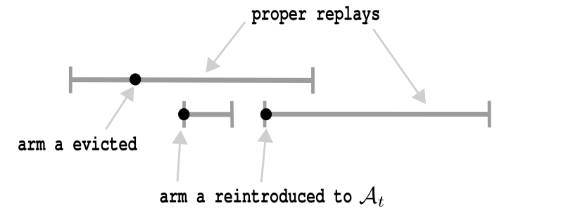
Figure 2: Shown are various replay scheduled durations (gray segments) with indications of when a given arm $a$ may be reintroduced to $\mathcal{A}_{t}$.

We first observe that for each round $t$ when a replay is active, there is a unique proper replay associated to $t$. This is either the replay active at round $t$ or the proper replay which was scheduled most recently before $t$. Then, for a fixed arm $a$, we partition the set of rounds $t>t_{\ell}^{a}$ where arm $a\in\mathcal{A}_{t}$ (and hence could be played) into intervals, each initiated by the start of a unique ${\small\textsf{{Base-Alg}}}(s,m)\in\textsc{Proper}(t_{\ell},t_{\ell+1})\cup\mathcal{R}(a)$ and terminated when arm $a$ is evicted or when the replay in question terminates, i.e. at round $M(s,m,a)$. Note that in this partition of rounds, it is not enough to merely consider the scheduling of proper replays ${\small\textsf{{Base-Alg}}}(s,m)\in\textsc{Proper}(t_{\ell},t_{\ell+1})$ since non-proper children of proper replays may resample arm $a$ after their parent evicts $a$. It is also not enough to consider just the schedules of replays in $\mathcal{R}(a)$, which reintroduce arm $a$, since a proper replay may not evict $a$ before being pre-empted by another proper replay. This delicate accounting of the rounds where arm $a$ is resampled is demonstrated in Figure 2.

Then, the second double sum in (10) can be decomposed into a sum over such replays and then a sum over the rounds where each such replay retains arm $a$. In other words, we can write the second double sum of (10) as:

$$\sum_{a=1}^{K}\sum_{{\small\textsf{{Base-Alg}}}(s,m)\in\textsc{Proper}(t_{\ell},t_{\ell+1})\cup\mathcal{R}(a)}\boldsymbol{1}\{B_{s,m}=1\}\sum_{t=s\vee t_{\ell}^{a}}^{M(s,m,a)}\frac{\delta_{t}(a_{\ell},a)}{|\mathcal{A}_{t}|}.$$

Further bounding the sum over $t$ above by its positive part, we can sum over all ${\small\textsf{{Base-Alg}}}(s,m)$, or obtain:

$$\sum_{a=1}^{K}\sum_{{\small\textsf{{Base-Alg}}}(s,m)}\boldsymbol{1}\{B_{s,m}=1\}\left(\sum_{t=s\vee t_{\ell}^{a}}^{M(s,m,a)}\frac{\delta_{t}(a_{\ell},a)}{|\mathcal{A}_{t}|}\cdot\boldsymbol{1}\{a\in\mathcal{A}_{t}\}\right)_{+},$$ (11)

where the sum is over all replays ${\small\textsf{{Base-Alg}}}(s,m)$, i.e. $s\in\{t_{\ell}+1,\ldots,t_{\ell+1}-1\}$ and $m\in\{2,4,\ldots,2^{\lceil\log(T)\rceil}\}$. It then remains to bound the contributed relative regret of each ${\small\textsf{{Base-Alg}}}(s,m)$ in the interval $[s\vee t_{\ell}^{a},M(s,m,a)]$, which will follow similarly to the previous steps. Fix $s,m$ and suppose $t_{\ell}^{a}+1\leq M(s,m,a)$ since otherwise ${\small\textsf{{Base-Alg}}}(s,m)$ contributes no regret in (11).

Then, following similar reasoning as before, i.e. combining our concentration bound (4) with the eviction criterion (2), we have for a fixed arm $a$:

$$\sum_{t=s\vee t_{\ell}^{a}}^{M(s,m,a)}\frac{\delta_{t}(a_{\ell},a)}{|\mathcal{A}_{t}|}\leq\frac{c_{5}\log(T)\sqrt{Km\vee K^{2}}}{\min_{t\in[s,M(s,m,a)]}|\mathcal{A}_{t}|},$$

Plugging this into (11) and switching the ordering of the outer double sum, we obtain

$$\sum_{{\small\textsf{{Base-Alg}}}(s,m)}c_{5}\log(T)\sqrt{Km\vee K^{2}}\sum_{a=1}^{K}\frac{1}{\min_{t\in[s,M(s,m,a)]}|\mathcal{A}_{t}|}.$$

We claim this inner sum over $a$ is at most $\log(K)$. For a fixed ${\small\textsf{{Base-Alg}}}(s,m)$, if $a_{k}$ is the $k$-th arm in $[K]$ to be evicted by ${\small\textsf{{Base-Alg}}}(s,m)$ or any of its children, then $\min_{t\in[s,M(s,m,a_{k})]}|\mathcal{A}_{t}|\geq K+1-k$. Thus, our claim follows follows from $\sum_{k=1}^{K}\frac{1}{K+1-k}\leq\log(K)$.

Let $R(m)\doteq c_{5}\log(K)\log(T)\sqrt{Km\vee K^{2}}$ which is the bound we’ve obtained so far on the relative regret for a single ${\small\textsf{{Base-Alg}}}(s,m)$. Then, plugging $R(m)$ into (11) gives:

$$\mathbb{E} \left[\boldsymbol{1}\{\mathcal{E}_{1}\}\sum_{a=1}^{K}\sum_{t=t_{\ell}^{a}}^{t_{\ell+1}-1}\frac{\delta_{t}(a_{\ell},a)}{|\mathcal{A}_{t}|}\cdot\boldsymbol{1}\{a\in\mathcal{A}_{t}\}\right]\leq\mathbb{E}_{t_{\ell}}\left[\mathbb{E}\left[\sum_{{\small\textsf{{Base-Alg}}}(s,m)}\boldsymbol{1}\{B_{s,m}=1\}\cdot R(m)\mid t_{\ell}\right]\right]$$

$$=\mathbb{E}_{t_{\ell}}\left[\sum_{s=t_{\ell+1}}^{T}\sum_{m}\mathbb{E}[\boldsymbol{1}\{B_{s,m}=1\}\cdot\boldsymbol{1}\{s<t_{\ell+1}\}\mid t_{\ell}]\cdot R(m)\right].$$

Next, we observe that $B_{s,m}$ and $\boldsymbol{1}\{s<t_{\ell+1}\}$ are independent conditional on $t_{\ell}$ since $\boldsymbol{1}\{s<t_{\ell+1}\}$ only depends on the scheduling and observations of base algorithms scheduled before round $s$. Thus, recalling that $\mathbb{P}(B_{s,m}=1)=1/\sqrt{m\cdot(s-t_{\ell})}$,

$$\mathbb{E}[\boldsymbol{1}\{B_{s,m}=1\}\cdot\boldsymbol{1}\{s<t_{\ell+1}\}\mid t_{\ell}] =\mathbb{E}[\boldsymbol{1}\{B_{s,m}=1\}\mid t_{\ell}]\cdot\mathbb{E}[\boldsymbol{1}\{s<t_{\ell+1}\}\mid t_{\ell}]$$

$$=\frac{1}{\sqrt{m\cdot(s-t_{\ell})}}\cdot\mathbb{E}[\boldsymbol{1}\{s<t_{\ell+1}\}\mid t_{\ell}].$$

Plugging this into our expectation from before and unconditioning, we obtain:

$$\mathbb{E}\left[\sum_{s=t_{\ell}+1}^{t_{\ell+1}-1}\sum_{n=1}^{\lceil\log(T)\rceil}\frac{1}{\sqrt{2^{n}\cdot(s-t_{\ell})}}\cdot R(2^{n})\right]\leq c_{6}\log^{3}(T)\mathbb{E}_{t_{\ell},t_{\ell+1}}\left[\sqrt{K(t_{\ell+1}-t_{\ell})\vee K^{2}}\right].$$ (12)

Then, to bound a, it suffices to bound $\sqrt{K(t_{\ell+1}-t_{\ell})\vee K^{2}}$. First, we claim that every phase $[\tau_{i},\tau_{i+1})$ is length at least $K/4$. Observe by our notion of significant regret, that an arm $a$ incurring significant regret on the interval $[s_{1},s_{2}]$ means

$$\sum_{t=s_{1}}^{s_{2}}\delta_{t}(a)\geq\sqrt{K\cdot(s_{2}-s_{1})}\implies 2\cdot(s_{2}-s_{1})\geq\sqrt{K\cdot(s_{2}-s_{1})}\implies s_{2}-s_{1}\geq K/4.$$

Thus, each significant phase (Definition 1) must be at least $K/4$ rounds long meaning $\tau_{i+1}-\tau_{i}=(\tau_{i+1}-\tau_{i})\vee K/4$.

Showing a is order (6) then follows from conditioning again on $\mathcal{E}_{1}$ in (12) and upper bounding $t_{\ell+1}-t_{\ell}$ by the combined length of all phases $[\tau_{i},\tau_{i+1})$ intersecting episode $[t_{\ell},t_{\ell+1})$.

B.2 Bounding $\mathbb{E}[\sum_{t=t_{\ell}}^{t_{\ell+1}-1}\delta_{t}(a_{t}^{\sharp},a_{\ell})]$ (Term b of Equation (7))

To show Proposition 10, we first need an elementary lemma which only depends on the definition of significant shift (Definition 1).

Lemma B.2.

Let $[s_{i,j}(a),s_{i,j+1}(a))$ be a bad segment, defined with respect to arm $a$. Then

$$\sum_{t=\left\lceil\frac{s_{i,j}(a)+s_{i,j+1}(a)}{2}\right\rceil}^{s_{i,j+1}(a)}\delta_{t}(a_{i}^{\sharp},a)\geq\frac{c_{4}}{4}\log(T)\sqrt{K\left(s_{i,j+1}(a)-\left(\frac{s_{i,j}(a)+s_{i,j+1}(a)}{2}\right)\right)}.$$ (13)

Proof B.3.

(of Lemma B.2) Let $\tilde{s}\doteq\left\lceil\frac{s_{i,j}(a)+s_{i,j+1}(a)}{2}\right\rceil$ be the midpoint between $s_{i,j}(a)$ and $s_{i,j+1}(a)$. Then, we have by (8) in the construction of the $s_{i,j}(a)$’s (Definition 9) that:

$$\sum_{t=\tilde{s}}^{s_{i,j+1}(a)}\delta_{t}(a_{i}^{\sharp},a) =\sum_{t=s_{i,j}(a)}^{s_{i,j+1}(a)}\delta_{t}(a_{i}^{\sharp},a)-\sum_{t=s_{i,j}(a)}^{\tilde{s}-1}\delta_{t}(a_{i}^{\sharp},a)$$

$$\geq c_{4}\log(T)\sqrt{K}\left(\sqrt{s_{i,j+1}(a)-s_{i,j}(a)}-\sqrt{\tilde{s}-1-s_{i,j}(a)}\right)$$

$$\geq\frac{c_{4}}{4}\log(T)\sqrt{K(s_{i,j+1}(a)-\tilde{s})},$$ (14)

where the last step is from the elementary fact $\sqrt{a+b}-\sqrt{a}\geq\sqrt{b}/4$ for any $b\geq a\geq 0$.

Proof B.4.

(of Proposition 10) Suppose event $\mathcal{E}_{1}$ (i.e., our concentration bound (4)) holds. For i, if ${\small\textsf{{Base-Alg}}}(\operatorname{\it{t}_{{\text{start}}}},m)$ with $\operatorname{\it{t}_{{\text{start}}}}\geq s_{i,j}(a)$ evicts arm $a_{i}^{\sharp}$ before round $s_{i,j+1}(a)$, then arm $a_{i}^{\sharp}$ incurs significant regret ($\star$ ‣ 2) on a subinterval of $[s_{i,j}(a),s_{i,j+1}(a)]$, which is a contradiction to the definition of arm $a_{i}^{\sharp}$.

For ii, we first observe $\mathbb{E}[\hat{\delta}_{t}(a_{i}^{\sharp},a)\mid\mathcal{F}_{t-1}]=\delta_{t}(a_{i}^{\sharp},a)$ for any round $t\in[\tilde{s},s_{i,j+1}(a)]$ if $a_{i}^{\sharp},a\in\mathcal{A}_{t}$. Then, combining (13) of Lemma B.2 with our concentration bound (4), we have that arm $a$ will satisfy the eviction criterion (2) over interval $[\tilde{s},s_{i,j+1}(a)]$.

Next, following the outline of Section 5.4, we bound the the regret of a fixed arm $a$ to $a_{i}^{\sharp}$ over the bad segments w.r.t. $a$. It should be understood that in what follows, we condition on $t_{\ell}$. First, fix an arm $a$ and define the bad round $s(a)>t_{\ell}$ as the smallest round which satisfies, for some fixed $c_{7}>0$:

$$\sum_{(i,j)}\sqrt{s_{i,j+1}(a)-s_{i,j}(a)}>c_{7}\log(T)\sqrt{s(a)-t_{\ell}},$$ (15)

where the above sum is over all pairs of indices $(i,j)\in\mathbb{N}\times\mathbb{N}$ such that $[s_{i,j}(a),s_{i,j+1}(a))$ is a bad segment with $s_{i,j+1}(a)<s(a)$. We will show that arm $a$ is evicted within episode $\ell$ with high probability by the time the bad round $s(a)$ occurs.

For each bad segment $[s_{i,j}(a),s_{i,j+1}(a))$, let $\tilde{s}_{i,j}(a)\doteq\left\lceil\frac{s_{i,j}(a)+s_{i,j+1}(a)}{2}\right\rceil$ denote the midpoint of the bad segment and also let $m_{i,j}\doteq 2^{n}$ where $n\in\mathbb{N}$ satisfies:

$$2^{n}\geq s_{i,j+1}(a)-s_{i,j}(a)>2^{n-1}.$$

Next, recall that the Bernoulli $B_{m.t}$ decides whether ${\small\textsf{{Base-Alg}}}(t,m)$ activates at round $t$ (see Line 4 of Algorithm 4). If for some $t\in[s_{i,j}(a),\tilde{s}_{i,j}(a)]$, $B_{t,m_{i,j}}=1$, i.e. a perfect replay is scheduled, then $a$ will be evicted from $\operatorname{\mathcal{A}_{\text{master}}}$ by round $s_{i,j+1}(a)$ (Corollary 12). We will show this happens with high probability via concentration on the sum $\sum_{(i,j)}\sum_{t}B_{t,m_{i,j}}$ where $j,i,t$ run through all $t\in[s_{i,j}(a),\tilde{s}_{i,j}(a))$ and all bad segments $[s_{i,j}(a),s_{i,j+1}(a))$ with $s_{i,j+1}(a)<s(a)$. Note that these random variables only depend on the fixed arm $a$, the episode start time $t_{\ell}$, and the randomness of scheduling replays on Line 4. In particular, the $B_{t,m_{i,j}}$ are independent conditional on $t_{\ell}$.

Then, a Chernoff bound over the randomization of META on Line 4 of Algorithm 4 conditional on $t_{\ell}$ yields

$$\mathbb{P}\left(\sum_{(i,j)}\sum_{t}B_{t,m_{i,j}}\leq\frac{\mathbb{E}[\sum_{(i,j)}\sum_{t}B_{t,m_{i,j}}\mid t_{\ell}]}{2}\mid t_{\ell}\right)\leq\exp\left(-\frac{\mathbb{E}[\sum_{(i,j)}\sum_{t}B_{t,m_{i,j}}\mid t_{\ell}]}{8}\right).$$

We claim the error probability on the R.H.S. above is at most $1/T^{3}$. To this end, we compute:

$$\mathbb{E}\left[\sum_{(i,j)}\sum_{t}B_{t,m_{i,j}}\mid t_{\ell}\right] \geq\displaystyle\sum_{(i,j)}\sum_{t=s_{i,j}(a)}^{\tilde{s}_{i,j}(a)}\frac{1}{\sqrt{m_{i,j}\cdot(t-t_{\ell})}}\geq\frac{1}{4}\displaystyle\sum_{(i,j)}\sqrt{\frac{s_{i,j+1}(a)-s_{i,j}(a)}{s(a)-t_{\ell}}}\geq\frac{c_{7}}{4}\log(T),$$

where the last inequality follows from (15). The R.H.S. above is larger than $24\log(T)$ for $c_{7}$ large enough, showing that the error probability is small. Taking a further union bound over the choice of arm $a\in[K]$ gives us that $\sum_{(i,j)}\sum_{t}B_{t,m_{i,j}}>1$ for all choices of arm $a$ (define this as the good event $\mathcal{E}_{2}(t_{\ell})$) with probability at least $1-K/T^{3}$.

Recall on the event $\mathcal{E}_{1}$ the concentration bounds of Proposition 6 hold. Then, on $\mathcal{E}_{1}\cap\mathcal{E}_{2}(t_{\ell})$, we must have $t_{\ell+1}-1\leq s(a_{\ell})$ since otherwise $a_{\ell}$ would have been evicted by some perfect replay before the end of the episode $t_{\ell+1}-1$ by virtue of $\sum_{(i,j)}\sum_{t}B_{t,m_{i,j}}>1$ for arm $a_{\ell}$. Thus, by the definition of the bad round $s(a_{\ell})$ (15), we must have:

$$\sum_{[s_{i,j}(a_{\ell}),s_{i,j+1}(a_{\ell})):s_{i,j+1}(a_{\ell})<t_{\ell+1}-1}\sqrt{s_{i,j+1}(a_{\ell})-s_{i,j}(a_{\ell})}\leq c_{7}\log(T)\sqrt{t_{\ell+1}-t_{\ell}}.$$ (16)

Thus, by (8) in Definition 9, over the bad segments $[s_{i,j}(a_{\ell}),s_{i,j+1}(a_{\ell}))$ which elapse before the end of the episode $t_{\ell+1}-1$, the regret of $a_{\ell}$ to $a_{t}^{\sharp}$ is at most order $\log^{2}(T)\sqrt{K\cdot(t_{\ell+1}-t_{\ell})}$.

Over each non-bad critical segment $[s_{i,j}(a_{\ell}),s_{i,j+1}(a_{\ell}))$ and the last segment $[s_{i,j}(a_{\ell}),t_{\ell+1}-1)$, the regret of playing arm $a_{\ell}$ to $a_{i}^{\sharp}$ is at most $\log(T)\sqrt{\tau_{i+1}-\tau_{i}}$ since there is at most one non-bad critical segment per phase $[\tau_{i},\tau_{i+1})$ (see (8) in Definition 9).

So, we conclude that on event $\mathcal{E}_{1}\cap\mathcal{E}_{2}(t_{\ell})$:

$$\sum_{t=t_{\ell}}^{t_{\ell+1}-1}\delta_{t}(a_{t}^{\sharp},a_{\ell})\leq c_{8}\log^{2}(T)\sum_{i\in\textsc{Phases}(t_{\ell},t_{\ell+1})}\sqrt{K(\tau_{i+1}-\tau_{i})}.$$

Taking expectation, we have by conditioning first on $t_{\ell}$ and then on event $\mathcal{E}_{1}\cap\mathcal{E}_{2}(t_{\ell})$:

$$\mathbb{E}\left[\sum_{t=t_{\ell}}^{t_{\ell+1}-1}\delta_{t}(a_{t}^{\sharp},a_{\ell})\right] \leq\mathbb{E}_{t_{\ell}}\left[\mathbb{E}\left[\boldsymbol{1}\{\mathcal{E}_{1}\cap\mathcal{E}_{2}(t_{\ell})\}\sum_{t=t_{\ell}}^{t_{\ell+1}-1}\delta_{t}(a_{t}^{\sharp},a_{\ell})\mid t_{\ell}\right]\right]+T\cdot\mathbb{E}_{t_{\ell}}\left[\mathbb{E}\left[\boldsymbol{1}\{\mathcal{E}_{1}^{c}\cup\mathcal{E}_{2}^{c}(t_{\ell})\}\mid t_{\ell}\right]\right]$$

$$\leq c_{8}\log^{2}(T)\mathbb{E}_{t_{\ell}}\left[\mathbb{E}\left[\boldsymbol{1}\{\mathcal{E}_{1}\cap\mathcal{E}_{2}(t_{\ell})\}\sum_{i\in\textsc{Phases}(t_{\ell},t_{\ell+1})}\sqrt{K(\tau_{i+1}-\tau_{i}})\mid t_{\ell}\right]\right]+\frac{K}{T^{2}}$$

$$\leq c_{8}\log^{2}(T)\mathbb{E}\left[\boldsymbol{1}\{\mathcal{E}_{1}\}\sum_{i\in\textsc{Phases}(t_{\ell},t_{\ell+1})}\sqrt{\tau_{i+1}-\tau_{i}}\right]+\frac{1}{T},$$

where in the last step we bound $\boldsymbol{1}\{\mathcal{E}_{1}\cap\mathcal{E}_{2}(t_{\ell})\}\leq\boldsymbol{1}\{\mathcal{E}_{1}\}$ and apply tower law again. This shows b is at most order the R.H.S. of (6). $\hfill\blacksquare$

Appendix C Proof of Corollary 3

The proof of Corollary 3 follows straightforwardly from Definition 1. Recall from Section 3 that $V\doteq\sum_{t=2}^{T}\max_{a\in[K]}|\mu_{t}(a)-\mu_{t-1}(a)|$ is the total variation of change in the rewards. Then, by Theorem 1, it suffices to show

$$\sum_{i=0}^{{\tilde{L}}}\sqrt{K(\tau_{i+1}-\tau_{i})}\lesssim\sqrt{KT}+(KV)^{1/3}\cdot T^{2/3}.$$ (17)

Fix a phase $[\tau_{i},\tau_{i+1})$ such that $\tau_{i+1}<T+1$. We first bound the total variation over this phase

$$V_{[\tau_{i},\tau_{i+1})}\doteq\sum_{t=\tau_{i}+1}^{\tau_{i+1}}\max_{a\in[K]}|\mu_{t}(a)-\mu_{t-1}(a)|.$$

By the definition of significant shift (Definition 1), an arm $a=\operatorname{argmax}_{a\in[K]}\mu_{\tau_{i+1}}(a)$ must incur significant regret ($\star$ ‣ 2) on the interval $[s_{1},s_{2}]$ for some $\tau_{i}\leq s_{1}<s_{2}<\tau_{i+1}$, or

$$\sum_{t=s_{1}}^{s_{2}}\delta_{t}(a)\geq\sqrt{K(s_{2}-s_{1})}.$$

Since $\sqrt{s_{2}-s_{1}}>\sum_{t=s_{1}}^{s_{2}}1/\sqrt{\tau_{i+1}-\tau_{i}}$, there must be a round $t\in[s_{1},s_{2}]$ such that $\delta_{t}(a)\geq\sqrt{K/(\tau_{i+1}-\tau_{i})}$. Let $a^{\prime}\in\operatorname{argmax}_{a^{\prime}\in[K]}\mu_{t}(a^{\prime})$. Then, we have

$$\sqrt{\frac{K}{\tau_{i+1}-\tau_{i}}}\leq\delta_{t}(a) \leq\mu_{t}(a^{\prime})-\mu_{t}(a)+\mu_{\tau_{i+1}}(a)-\mu_{\tau_{i+1}}(a^{\prime})$$

$$\leq|\mu_{\tau_{i+1}}(a)-\mu_{t}(a)|+|\mu_{t}(a^{\prime})-\mu_{\tau_{i+1}}(a^{\prime})|$$

$$\leq 2\sum_{s=t+1}^{\tau_{i+1}}\max_{a\in[K]}|\mu_{s}(a)-\mu_{s-1}(a)|$$

$$\leq 2\cdot V_{[\tau_{i},\tau_{i+1})}$$

This gives us a lower bound on the total variation over each interval $[\tau_{i},\tau_{i+1})$. Then, by Hölder’s inequality:

$$\sum_{i=0}^{{\tilde{L}}}\sqrt{K(\tau_{i+1}-\tau_{i})} =\sqrt{K(T+1-\tau_{{\tilde{L}}})}+\sum_{i=0}^{\tilde{L}-1}\sqrt{K(\tau_{i+1}-\tau_{i})}$$

$$\leq\sqrt{KT}+\left(\sum_{i=0}^{{\tilde{L}}}\sqrt{\frac{K}{\tau_{i+1}-\tau_{i}}}\right)^{1/3}\left(\sum_{i=0}^{{\tilde{L}}}(\tau_{i+1}-\tau_{i})\sqrt{K}\right)^{2/3}$$

$$\leq\sqrt{KT}+\left(\sum_{i=0}^{{\tilde{L}}}2V_{[\tau_{i},\tau_{i+1})}\right)^{1/3}K^{1/3}T^{2/3}$$

$$=\sqrt{KT}+(2KV)^{1/3}\cdot T^{2/3}.$$

$\hfill\blacksquare$

References

- Abbasi-Yadkori et al. (2022) Yasin Abbasi-Yadkori, András György, and Nevena Lazic. A new look at dynamic regret for non-stationary stochastic bandits. arXiv preprint arXiv:2201.06532, 2022. URL https://arxiv.org/pdf/2201.06532.pdf.
- Allesiardo et al. (2017) Robin Allesiardo, Raphaël Féraud, and Odalric-Ambrym Maillard. The non-stationary stochastic multi-armed bandit problem. International Journal of Data Science and Analytics, 3(4):267–283, 2017.
- Auer (2002) Peter Auer. Using confidence bounds for exploitation-exploration trade-offs. Journal of Machine Learning Research, 3:397–422, 2002.
- Auer and Chiang (2016) Peter Auer and Chao-Kai Chiang. An algorithm with nearly optimal pseudo-regret for both stochastic and adversarial bandits. Proceedings of the 29th Conference on Learning Theory, COLT 2016, pages 116–120, 2016.
- Auer et al. (2002) Peter Auer, Nicolo Cesa-Bianchi, Yoav Freund, and Robert E Schapire. The nonstochastic multiarmed bandit problem. SIAM journal on computing, 32(1):48–77, 2002.
- Auer et al. (2018) Peter Auer, Pratik Gajane, and Ronald Ortner. Adaptively tracking the best arm with an unknown number of distribution changes. 14th European Workshop on Reinforcement Learning (EWRL), 2018.
- Auer et al. (2019) Peter Auer, Pratik Gajane, and Ronald Ortner. Adaptively tracking the best bandit arm with an unknown number of distribution changes. Conference on Learning Theory, pages 138–158, 2019.
- Besson et al. (2022) Lilian Besson, Emilie Kaufmann, Odalric-Ambrym Maillard, and Julien Seznec. Efficient change-point detection for tackling piecewise-stationary bandits. The Journal of Machine Learning Research, 23(77):1–40, 2022.
- Beygelzimer et al. (2011) Alina Beygelzimer, John Langford, Lihong Li, Lev Reyzin, and Robert E. Schapire. Contextual bandit algorithms with supervised learning guarantees. AISTATS, 2011.
- Bubeck and Cesa-Bianchi (2012) Sébastien Bubeck and Nicoló Cesa-Bianchi. Regret analysis of stochastic and nonstochastic multi-armed bandit problems. arXiv preprint arXiv:1803.06971, 5(1), 2012.
- Bubeck and Slivkins (2012) Sébastien Bubeck and Aleksandrs Slivkins. The best of both worlds: Stochastic and adversarial bandits. The 25th Annual Conference on Learning Theory, (42):1–23, 2012.
- Chen et al. (2019) Yifang Chen, Chung-Wei Lee, Haipeng Luo, and Chen-Yu Wei. A new algorithm for non-stationary contextual bandits: Efficient, optimal and parameter-free. In Conference on Learning Theory, pages 696–726, 2019.
- Cheung et al. (2019) Wang Chi Cheung, David Simchi-Levi, and Ruihao Zhu. Learning to optimize under non-stationarity. In The 22nd International Conference on Artificial Intelligence and Statistics, pages 1079–1087. PMLR, 2019.
- Foster et al. (2020) Dylan J. Foster, Akshay Krishnamurthy, and Haipeng Luo. Open problem: Model selection for contextual bandits. 33rd Annual Conference on Learning Theory (COLT), 2020.
- Garivier and Moulines (2011) Aurélien Garivier and Eric Moulines. On upper-confidence bound policies for switching bandit problems. In Proceedings of the 22nd International Conference on Algorithmic Learning Theory, pages 174–188. ALT 2011, Springer, 2011.
- Heidari et al. (2016) Hoda Heidari, Michael Kearns, and Aaron Roth. Tight policy regret bounds for improving and decaying bandits. Proceedings of the International Joint Conference on Artificial Intelligence (IJCAI), pages 1562–1570, 2016.
- Kocsis and Szepesvári (2006) Levente Kocsis and Csaba Szepesvári. Discounted ucb. 2nd PASCAL Challenges Workshop, 2006.
- Krishnamurthy and Gopalan (2021) Ramakrishnan Krishnamurthy and Aditya Gopalan. On slowly-varying non-stationary bandits. arXiv preprint: arXiv:2110.12916, 2021. URL https://arxiv.org/pdf/2110.12916.pdf.
- Lattimore and Szepesvári (2020) Tor Lattimore and Csaba Szepesvári. Bandit Algoritms. Cambridge University Press, 2020.
- Levine et al. (2017) Nir Levine, Koby Crammer, and Shie Mannor. Rotting bandits. Advanced in Neural Information Processing Systems, 2017.
- Manegueu et al. (2021) Anne Gael Manegueu, Alexandra Carpentier, and Yi Yu. Generalized non-stationary bandits. arXiv preprint: arXiv:2102.00725, 2021. URL https://arxiv.org/pdf/2102.00725.pdf.
- Marinov and Zimmert (2021) Teodor Marinov and Julian Zimmert. The pareto frontier of model selection for general contextual bandits. Advances in Neural Information Processing Systems, 2021.
- Mukherjee and Maillard (2019) Subhojyoti Mukherjee and Odalric-Ambrym Maillard. Distribution-dependent and time-uniform bounds for piecewise i.i.d bandits. Reinforcement Learning for Real Life (RL4RealLife) Workshop in the 36th International Conference on Mearning Learning, 2019.
- Seldin and Slivkins (2014) Yevgeny Seldin and Aleksandrs Slivkins. One practical algorithm for both stochastic and adversarial bandits. Proceedings of the 31st International Conference on Machine Learning (ICML), 2014.
- Seznec et al. (2019) Julien Seznec, Andrea Locatelli, Alexandra Carpentier, Alessandro Lazaric, and Michal Valko. Rotting bandits are no harder than stochastic ones. Proceedings of the Twenty-Second International Conference on Artificial Intelligence and Statistics, pages 2564–2572, 2019.
- Seznec et al. (2020) Julien Seznec, Pierre Menard, Alessandro Lazaric, and Michal Valko. A single algorithm for both restless and rested rotting bandits. Proceedings of the 22nd International Conference on Artificial Intelligence and Statistics (AISTATS), 2020.
- Slivkins (2019) Aleksandrs Slivkins. Introduction to Multi-Armed Bandits. 2019. URL https://arxiv.org/abs/1904.07272.
- Slivkins and Upfal (2008) Alex Slivkins and Eli Upfal. Adapting to a changing environment: the brownian restless bandits. 21st Conference on Learning Theory (COLT), 2008.
- Wei and Luo (2021) Chen-Yu Wei and Haipeng Luo. Non-stationary reinforcement learning without prior knowledge: An optimal black-box approach. Proceedings of the 32nd International Conference on Learning Theory, 2021.
- Wei and Srivatsva (2018) Lai Wei and Vaihbav Srivatsva. On abruptly-changing and slowly-varying multiarmed bandit problems. Annual American Control Conference (ACC), 2018.