Implicit regularity and linear convergence rates for the generalized trust-region subproblem

Abstract

In this paper we develop efficient first-order algorithms for the generalized trust-region subproblem (GTRS), which has applications in signal processing, compressed sensing, and engineering. Although the GTRS, as stated, is nonlinear and nonconvex, it is well-known that objective value exactness holds for its SDP relaxation under a Slater condition. While polynomial-time SDP-based algorithms exist for the GTRS, their relatively large computational complexity has motivated and spurred the development of custom approaches for solving the GTRS. In particular, recent work in this direction has developed first-order methods for the GTRS whose running times are linear in the sparsity (the number of nonzero entries) of the input data. In contrast to these algorithms, in this paper we develop algorithms for computing $\epsilon$-approximate solutions to the GTRS whose running times are linear in both the input sparsity and the precision $\log(1/\epsilon)$ whenever a regularity parameter is positive. We complement our theoretical guarantees with numerical experiments comparing our approach against algorithms from the literature. Our numerical experiments highlight that our new algorithms significantly outperform prior state-of-the-art algorithms on sparse large-scale instances.

1 Introduction

In this paper we develop efficient first-order algorithms for the generalized trust-region subproblem (GTRS). Recall the GTRS,

$$\operatorname{Opt}\coloneqq\inf_{x\in{\mathbb{R}}^{n}}\left\{q_{0}(x):\,q_{1}(x)\leq 0\right\},$$

where $q_{0}(x)$ and $q_{1}(x)$ are quadratic functions in $x\in{\mathbb{R}}^{n}$. We will assume that for each $i\in\left\{0,1\right\}$, the quadratic function $q_{i}(x)$ is given by $q_{i}(x)=x^{\top}A_{i}x+2b_{i}^{\top}x+c_{i}$ for $A_{i}\in{\mathbb{S}}^{n}$, $b_{i}\in{\mathbb{R}}^{n}$ and $c_{i}\in{\mathbb{R}}$.

This problem generalizes the classical trust-region subproblem (TRS) where the general quadratic constraint $q_{1}(x)\leq 0$ is replaced with the unit ball constraint $\left\lVert x\right\rVert^{2}\leq 1$. The TRS finds applications, for example, in robust optimization [2, 16] and combinatorial optimization [28, 22]. The TRS is additionally foundational in the area of nonlinear programming. Indeed, iterative algorithms based on the TRS (known sometimes as trust-region methods) [6] are among the most empirically successful techniques for general nonlinear programs.

Generalizing the TRS, the GTRS has applications in signal processing, compressed sensing, and engineering (see [34] and references therein). The problem of minimizing a quartic of the form $q(x,p(x))$, where $q:{\mathbb{R}}^{n+1}\to{\mathbb{R}}$ and $p:{\mathbb{R}}^{n}\to{\mathbb{R}}$ are both quadratic, can be cast in the equality-constrained variant of the GTRS. This approach has been used to address source localization [15] as well as the double-well potential functions [9]. More broadly, iterative ADMM-based algorithms for general QCQPs using the GTRS as a subprocedure have shown exceptional numerical performance [17] and outperform previous state-of-the-art approaches on a number of real world problems (e.g., multicast beamforming and phase retrieval). This application of the GTRS as a subprocedure within an iterative solver parallels the use of the TRS within trust-region methods.

Although the GTRS, as stated, is nonlinear and nonconvex, it is well-known that objective value exactness holds for its SDP relaxation under a Slater condition [11, 29]. Thus, unlike general QCQPs which are NP-hard, the GTRS can be solved in polynomial time via SDP-based algorithms. Nevertheless, the relatively large computational complexity of SDP-based approaches has motivated and spurred the development of alternative custom approaches for solving the GTRS. We restrict our discussion below to recent trends in GTRS algorithms and discuss earlier work [25, 26, 32] where appropriate in the main body.

One line of proposed algorithms for the GTRS assumes simultaneous diagonalizability (SD) of $A_{0}$ and $A_{1}$. It is well-known that SD holds under minor conditions—for example, if there exists a positive definite matrix in $\operatorname{span}\left\{A_{0},A_{1}\right\}$ (see [33] for additional variants of this result). Ben-Tal and Teboulle [4] exploit the SD condition to provide a reformulation of the interval-constrained GTRS as a convex minimization problem with linear constraints. More recently, under the SD condition, Ben-Tal and den Hertog [2] provide a second-order cone program (SOCP) reformulation of the GTRS in a lifted space. This SOCP reformulation was generalized beyond the GTRS in [24]. Under the SD condition, a number of papers [31, 8] exploit the resulting problem structure of the primal or the dual formulation to derive solution procedures for the GTRS and interval-constrained GTRS. Generalizing [2], Jiang et al. [21] provide an SOCP reformulation for the GTRS in a lifted space whenever the problem has a finite optimal value even when the SD condition fails. Unfortunately, the algorithms in this line often assume implicitly that $A_{0}$ and $A_{1}$ are already diagonal or that a simultaneously-diagonalizing basis can be computed. In practice, however, computing such a basis requires a full eigen-decomposition and can be prohibitively expensive for large-scale instances.

A second line of research on the GTRS explores the connection between the GTRS and generalized eigenvalues of the matrix pencil $A_{0}+\gamma A_{1}$. Pong and Wolkowicz [30] propose a generalized-eigenvalue-based algorithm which exploits the structure of optimal GTRS solutions, albeit without an explicit running time analysis. Adachi and Nakatsukasa [1] present another approach for solving the GTRS based on computing the minimum generalized eigenvalue (and corresponding eigenvector) of an associated indefinite $(2n+1)\times(2n+1)$ matrix pencil. Unfortunately, this approach suffers from the significant cost of computing a minimum generalized eigenvalue of an indefinite matrix pencil. Empirically, the complexity of this approach scales as $O(n^{2})$ even for sparse instances of the GTRS with $O(n)$ nonzero entries in $A_{0}$ and $A_{1}$ (see [1, Section 4]). Jiang and Li [19] reformulate the GTRS as the problem of minimizing the maximum of two convex quadratic functions in the original space. This reformulation is constructed from a pair of generalized eigenvalues related to the matrix pencil $A_{0}+\gamma A_{1}$. They then suggest a saddle-point-based first-order algorithm to solve this reformulation within an $\epsilon$ additive error in $O(1/\epsilon)$ time. These approaches are based on the assumption that the generalized eigenvalues are given or can be computed exactly, and offer no theoretical guarantees when only approximate generalized eigenvalue computations are available (as is the case in practice; see also the discussion in Section 4.1 in [20]). Despite this, the numerical experiments in [19, 1, 30] suggest that algorithms motivated by these ideas perform well even using only approximate generalized eigenvalue computations.

In contrast to these papers, recent work [20, 34] offers provably linear-time (in terms of the number of nonzero entries in the input data) algorithms for the GTRS using only approximate eigenvalue procedures. Jiang and Li [20] extend ideas developed in [14] for solving the TRS to derive an algorithm for solving the GTRS up to an $\epsilon$ additive error with high probability. This approach differs from the earlier literature in that it does not rely on the computation of a simultaneously-diagonalizing basis or exact generalized eigenvalues. The complexity of this approach is

$$\tilde{O}\left(\frac{N}{\sqrt{\epsilon}}\log\left(\frac{n}{p}\right)\log\left(\frac{1}{\epsilon}\right)^{2}\right),$$

where $N$ is the number of nonzero entries in $A_{0}$ and $A_{1}$, $\epsilon$ is the additive error, and $p$ is the failure probability. Here, we have elided quantities related to the condition number of the GTRS. Wang and Kılınç-Karzan [34] reexamine the convex quadratic reformulation idea of [19] and show formally that by approximating the generalized eigenvalues sufficiently well, the perturbed convex reformulation is within a small additive error of the true convex reformulation. Moreover, they establish that the resulting convex reformulation can be solved via Nesterov’s accelerated gradient descent method [27, Section 2.3.3] for smooth minimax problems to achieve an overall run time guarantee of

$$\tilde{O}\left(\frac{N}{\sqrt{\epsilon}}\log\left(\frac{n}{p}\right)\log\left(\frac{1}{\epsilon}\right)\right).$$

A parallel line of work [16, 10, 13, 26, 14, 5] has developed custom first-order methods for the trust-region subproblem. Most relatedly, Carmon and Duchi [5] recently showed that a Krylov-based first-order method can achieve a convergence rate for the TRS that is linear in both $N$ and the precision $\log(1/\epsilon)$ whenever a regularity parameter, $\mu^{*}$, is positive. This contrasts with previous algorithms for the TRS whose guarantees scaled as $\approx 1/\sqrt{\epsilon}$.

In this paper, we introduce and analyze a new algorithm for computing an $\epsilon$-approximate solution to the GTRS whose running time is linear in both $N$ and the precision $\log(1/\epsilon)$ whenever $\mu^{*}$ is positive. To be concrete, an $\epsilon$-approximate solution is defined below.

Definition 1.

We say $x\in{\mathbb{R}}^{n}$ is an $\epsilon$-approximate solution to (1) if

$$q_{0}(x)\leq\operatorname{Opt}+\epsilon\quad\text{and}\quad q_{1}(x)\leq\epsilon.$$

Despite similar convergence guarantees, our approach for solving the GTRS does not share many algorithmic similarities with the approach of Carmon and Duchi [5] for the TRS.

1.1 Overview and outline of paper

A summary of our contributions, along with an outline of the remainder of the paper, is as follows:

• In Section 2, we recall definitions and results related to the Lagrangian dual of the GTRS and define our notion of regularity. Specifically, we recall definitions and results in the literature [25, 26, 1, 9] regarding the dual function $\mathbf{d}(\gamma)$ and its derivative $\nu(\gamma)$. We then define a regularity parameter $\mu^{*}$, which will play the role of strong convexity in our algorithms. We close with a key lemma (Lemma 3) that underpins the algorithms developed in this paper. Intuitively, Lemma 3 says that when $\mu^{*}$ is positive, the unique optimizer of the GTRS is stable—an $\Omega(\mu^{*})$-strongly convex reformulation of the GTRS, whose unique optimizer coincides with the GTRS optimizer, can be built using inexact estimates of the dual optimizer $\gamma^{*}$.

• In Section 3, we describe and analyze an approach for computing an $\epsilon$-approximate optimizer of a nonconvex-nonconvex GTRS instance based on Lemma 3. Our approach consists of two algorithms, ConstructReform and SolveRegular. The first algorithm uses inexact estimates of $\nu(\gamma)$ to binary search for an inexact estimate of $\gamma^{*}$. ConstructReform will either return an exact $\Omega(\mu^{*})$-strongly convex reformulation of the GTRS or an $\epsilon$-approximate optimizer of the GTRS. In the former case, we may then apply SolveRegular to compute an $\epsilon$-approximate optimizer. In the latter case, ConstructReform will additionally attempt to certify that $\mu^{*}=O(\epsilon)$ so that building an $\Omega(\mu^{*})$-strongly convex reformulation may be undesirable. Together, these two algorithms achieve the following linear convergence rate (i.e., scaling as $\log(1/\epsilon)$) for the GTRS:

  $$\tilde{O}\left(\frac{N}{\sqrt{\phi}}\log\left(\frac{1}{\phi}\right)\log\left(\frac{n}{p}\right)\log\left(\frac{1}{\epsilon}\right)\right).$$

  Here, $N$ is the number of nonzero entries in $A_{0}$ and $A_{1}$ combined, $\phi$ can be thought of as $\approx\max(\mu^{*},\epsilon)$ (see Section 3 for a formal definition), $p$ is the failure probability, and the $\tilde{O}$-notation hides $\log\log$-factors. This contrasts with previous algorithms [34, 20] that are described as “linear-time”, referring to the fact that their running times scale linearly in only $N$. We close this section by examining in further detail the case where ConstructReform returns an $\epsilon$-approximate optimizer but fails to certify that $\mu^{*}=O(\epsilon)$. Specifically, we show that this edge case can only happen if $\nu(\gamma)$ is “extremely flat,” which in turn can only happen if a certain coherence parameter is small.

• In Section 4, we present numerical experiments comparing the algorithms of Section 3 to other algorithms proposed in the recent literature [2, 19, 1]. Our numerical experiments corroborate our theoretical understanding of the situation—the algorithms in this paper significantly outperform prior state-of-the-art algorithms on sparse large-scale GTRS instances.

1.2 Notation

For $x\in{\mathbb{R}}$ and $y\geq 0$ let $[\pm y]\coloneqq[-y,+y]$ and $[x\pm y]\coloneqq[x-y,x+y]$. We denote the $i$-th unit vector in ${\mathbb{R}}^{n}$ by $e_{i}$. Let ${\mathbb{S}}^{n}$ denote the $n\times n$ real symmetric matrices. For $A\in{\mathbb{S}}^{n}$ we will write $A\succeq 0$ (resp. $A\succ 0$) to denote that $A$ is positive semidefinite (resp. positive definite). For $\gamma\in{\mathbb{R}}_{+}$, define $A(\gamma)\coloneqq A_{0}+\gamma A_{1}$, $b(\gamma)\coloneqq b_{0}+\gamma b_{1}$, and $c(\gamma)\coloneqq c_{0}+\gamma c_{1}$. Let $q(\gamma,x)\coloneqq q_{0}(x)+\gamma q_{1}(x)$. For $A\in{\mathbb{S}}^{n}$, let $\left\lVert A\right\rVert$ be its spectral norm. For $b\in{\mathbb{R}}^{n}$, let $\left\lVert b\right\rVert$ be its Euclidean norm. For an interval $\Gamma\subseteq{\mathbb{R}}$, let $\operatorname{int}(\Gamma)$ denote its interior. We will use $\tilde{O}$-notation to hide $\log\log$-factors in our running times.

2 Implicit Regularity in the GTRS

Recall that the GTRS is the problem of minimizing a quadratic objective function subject to a single quadratic constraint, i.e.,

$$\operatorname{Opt}\coloneqq\inf_{x\in{\mathbb{R}}^{n}}\left\{q_{0}(x):\,q_{1}(x)\leq 0\right\},$$ (1)

where for each $i\in\left\{0,1\right\}$, we have $q_{i}(x)=x^{\top}A_{i}x+2b_{i}^{\top}x+c_{i}$ for some $A_{i}\in{\mathbb{S}}^{n}$, $b_{i}\in{\mathbb{R}}^{n}$, and $c_{i}\in{\mathbb{R}}$.

We will make the following blanket assumption, which is both natural and common in the literature on the GTRS [34, 1, 18, 20]. This assumption can be thought of as primal and dual strict feasibility assumptions or a Slater assumption.

Assumption 1.

There exists $\bar{x}\in{\mathbb{R}}^{n}$ such that $q_{1}(\bar{x})<0$ and there exists $\bar{\gamma}\geq 0$ such that $A(\bar{\gamma})\succ 0$.

Remark 1.

Note, for example, that Assumption 1 holds in the classical TRS setting where $q_{1}(x)=x^{\top}x-1$. Indeed, $q_{1}(0)<0$ and $A(\gamma)=A_{0}+\gamma I\succ 0$ for all $\gamma$ large enough.

The results and definitions will assume only Assumption 1. In particular, they can be applied to both the classical TRS setting as well as the nonconvex-nonconvex GTRS setting of Section 3.

Let $\Gamma\coloneqq\left\{\gamma\in{\mathbb{R}}_{+}:\,A(\gamma)\succeq 0\right\}$. This is a closed interval as the positive semidefinite cone is closed. If $\Gamma$ is bounded, let $[\gamma_{-},\gamma_{+}]$ denote its left and right endpoints. Else, let $\gamma_{-}$ denote its left endpoint and define $\gamma_{+}\coloneqq+\infty$. Note that for any $\gamma\in\Gamma$, $q(\gamma,x)$ is a convex function of $x$. Furthermore, by the existence of $\bar{\gamma}\geq 0$ such that $A(\bar{\gamma})\succ 0$, we have that $0\leq\gamma_{-}<\gamma_{+}$.

Definition 2.

Let $\mathbf{d}:{\mathbb{R}}_{+}\to\left\{-\infty\right\}\cup{\mathbb{R}}$ denote the extended-real-valued function defined by

$$\mathbf{d}(\gamma) \coloneqq\inf_{x\in{\mathbb{R}}^{n}}q(\gamma,x).$$

We make the following observations on $\mathbf{d}(\gamma)$.

Observation 1.

Suppose Assumption 1 holds. Then,

• The function $\mathbf{d}(\gamma)$ is continuous and concave as it is the infimum of affine functions of $\gamma$.

• For $\gamma\in{\mathbb{R}}_{+}\setminus\Gamma$, the function $q(\gamma,x)$ is nonconvex in $x$ so that $\mathbf{d}(\gamma)=-\infty$.

• As $q_{1}(\bar{x})<0$, we have $\mathbf{d}(\gamma)\leq q(\gamma,\bar{x})\to-\infty$ as $\gamma\to\infty$.

We comment on the connection between $\mathbf{d}(\gamma)$, the SDP relaxation of (1), and the Lagrangian dual of (1). One consequence of the S-lemma [11] is that the GTRS has an exact SDP relaxation. Furthermore, it is well-known that the SDP relaxation of a general quadratically constrained quadratic program is equivalent to its Lagrangian dual [3]. We will write this fact in our setting as the following identity (which holds under Assumption 1),

$$\operatorname{Opt}=\inf_{x\in{\mathbb{R}}^{n}}\sup_{\gamma\in\Gamma}q(\gamma,x).$$ (2)

We provide a short self-contained proof of this fact in Appendix C. Next, by coercivity [7, Proposition VI.2.3] we have that

$$\operatorname{Opt}=\sup_{\gamma\in\Gamma}\inf_{x\in{\mathbb{R}}^{n}}q(\gamma,x)=\sup_{\gamma\in\Gamma}\mathbf{d}(\gamma)=\sup_{\gamma\in{\mathbb{R}}_{+}}\mathbf{d}(\gamma).$$ (3)

In words, (2) shows that the GTRS can be written as a convex minimization problem. Specifically, we can write $\operatorname{Opt}$ in one of the two following ways, corresponding respectively to the cases $\gamma_{+}<\infty$ and $\gamma_{+}=\infty$:

$$\operatorname{Opt}=\inf_{x\in{\mathbb{R}}^{n}}\max\left(q(\gamma_{-},x),q(\gamma_{+},x)\right)\quad\text{or}\quad\operatorname{Opt}=\inf_{x\in{\mathbb{R}}^{n}}\left\{q(\gamma_{-},x):\,q_{1}(x)\leq 0\right\}.$$ (4)

Note in the latter case that $A_{1}\succeq 0$ so that $q_{1}(x)\leq 0$ is a convex constraint. Similarly, (3) shows that the GTRS can be written as a concave maximization problem.

Remark 2.

The reformulation of the GTRS given in (4) immediately suggests an algorithm for approximating $\operatorname{Opt}$: Compute $\gamma_{-}$ (and if necessary $\gamma_{+}$) up to some accuracy and solve the resulting convex reformulation. Convergence guarantees along with rigorous error analyses for such an algorithm were previously explored by Wang and Kılınç-Karzan [34]. One drawback to this approach is that the convex functions $q(\gamma_{-},x)$ and $q(\gamma_{+},x)$ are, by construction, not both strongly convex unless $A_{0},A_{1}\succ 0$. Thus, in view of oracle lower bounds for first-order-methods [27, Chapter 2.1.2], one should not expect to achieve linear convergence rates via this approach. Similarly, the reformulation of the GTRS given in (3) immediately suggests an algorithm for approximating $\operatorname{Opt}$: apply a root-finding algorithm or binary search to find $\gamma^{*}$. This approach dates back to Moré and Sorenson [26] for the TRS and Moré [25] for the GTRS (see also [9, 1]). Unfortunately, theoretical convergence rates have not been established for algorithms of this form.

We will combine both ideas above to construct strongly convex reformulations for instances of (1) possessing regularity. Our notion of regularity will correspond to properties of $\mathbf{d}(\gamma)$ and its optimizers. We will need the following notation.

Definition 3.

For $\gamma\in\operatorname{int}(\Gamma)$, define

$$x(\gamma) \coloneqq-A(\gamma)^{-1}b(\gamma),\quad\nu(\gamma)\coloneqq q_{1}(x(\gamma)),\quad\text{and}\quad\mu(\gamma)\coloneqq\lambda_{\min}\left(A(\gamma)\right).$$

The functions $\mathbf{d}(\gamma)$, $x(\gamma)$, and $\nu(\gamma)$ have been studied previously in the literature on algorithms for the TRS and the GTRS [1, 26, 25, 9]. In contrast to previous algorithms in this line of work, which propose methods for computing $\gamma^{*}$ to high accuracy, the algorithms we present in this paper will work with relatively inaccurate estimates of $\gamma^{*}$. Specifically, our algorithms are inspired by a key lemma, namely Lemma 3, which says that if (1) has positive regularity, then the optimal solution to (1) is stable to inaccurate estimates of $\gamma^{*}$. We begin by deriving some properties of $\mathbf{d}(\gamma)$ and its derivatives on $\operatorname{int}(\Gamma)$.

Lemma 1.

Suppose Assumption 1 holds. If $\gamma\in\operatorname{int}(\Gamma)$, then

$$\mathbf{d}(\gamma)=q(\gamma,x(\gamma))\quad\text{and}\quad\tfrac{d}{d\gamma}\mathbf{d}(\gamma)=\nu(\gamma).$$

Proof.

For $\gamma\in\operatorname{int}(\Gamma)$, we have $A(\gamma)\succ 0$ and thus $q(\gamma,x)$ is a strongly convex quadratic function in $x$. One may check that $\nabla_{x}q(\gamma,x)=2\left(A(\gamma)x+b(\gamma)\right)$, and thus $\mathbf{d}(\gamma)=q(\gamma,x(\gamma))$.

Next, from $\mathbf{d}(\gamma)=q(\gamma,x(\gamma))$ and $x(\gamma)=-A(\gamma)^{-1}b(\gamma)$, we deduce

$$\tfrac{d}{d\gamma}\mathbf{d}(\gamma) =\tfrac{d}{d\gamma}\left(-b(\gamma)^{\top}A(\gamma)^{-1}b(\gamma)+c(\gamma)\right)$$

$$=b(\gamma)^{\top}A(\gamma)^{-1}A_{1}A(\gamma)^{-1}b(\gamma)-2b_{1}^{\top}A(\gamma)^{-1}b(\gamma)+c_{1}$$

$$=q_{1}(x(\gamma)).\qed$$

Lemma 2.

Suppose Assumption 1 holds. Let $\hat{\gamma}\in\operatorname{int}(\Gamma)$, $P\coloneqq A(\hat{\gamma})^{-1/2}$, and $\Delta\coloneqq(A_{0}P^{2}b_{1}-A_{1}P^{2}b_{0})$. Then, for $\gamma\in\operatorname{int}(\Gamma)$,

$$\tfrac{d}{d\gamma}\nu(\gamma) =-2\left(A_{1}x(\gamma)+b_{1}\right)^{\top}A(\gamma)^{-1}\left(A_{1}x(\gamma)+b_{1}\right)$$

$$=-2\Delta^{\top}\left(A(\gamma)P^{2}A(\gamma)P^{2}A(\gamma)\right)^{-1}\Delta.$$

Proof.

Starting from $\nu(\gamma)=q_{1}(x(\gamma))$, we compute

$$\tfrac{d}{d\gamma}\nu(\gamma) =\left\langle\nabla_{x}q_{1}(x)\mid_{x=x(\gamma)},\nabla_{\gamma}x(\gamma)\right\rangle$$

$$=-2\left\langle A_{1}x(\gamma)+b_{1},A(\gamma)^{-1}(A_{1}x(\gamma)+b_{1})\right\rangle$$

$$=-2(A_{1}x(\gamma)+b_{1})^{\top}A(\gamma)^{-1}(A_{1}x(\gamma)+b_{1}).$$

Note also that

$$A_{1}x(\gamma)+b_{1} =A(\gamma)A(\gamma)^{-1}b_{1}-A_{1}A(\gamma)^{-1}b(\gamma)$$

$$=\left(A_{0}A(\gamma)^{-1}b_{1}+\gamma A_{1}A(\gamma)^{-1}b_{1}\right)-\left(A_{1}A(\gamma)^{-1}b_{0}+\gamma A_{1}A(\gamma)^{-1}b_{1}\right)$$

$$=A_{0}A(\gamma)^{-1}b_{1}-A_{1}A(\gamma)^{-1}b_{0}.$$

Next, suppose $\hat{\gamma}\in\operatorname{int}(\Gamma)$ and let $P\coloneqq A(\hat{\gamma})^{-1/2}$. Then, $PA_{0}P$ and $PA_{1}P$ commute. Indeed, $PA_{0}P+\hat{\gamma}PA_{1}P=PA(\hat{\gamma})P=I$. Then,

$$A_{0}A(\gamma)^{-1}b_{1} =P^{-1}PA_{0}P(PA(\gamma)P)^{-1}Pb_{1}$$

$$=P^{-1}(PA(\gamma)P)^{-1}PA_{0}P^{2}b_{1}$$

$$=(A(\gamma)P^{2})^{-1}A_{0}P^{2}b_{1}.$$

Similarly, $A_{1}A(\gamma)^{-1}b_{0}=(A(\gamma)P^{2})^{-1}A_{1}P^{2}b_{0}$. We deduce

$$\tfrac{d}{d\gamma}\nu(\gamma) =-2\left(A_{0}P^{2}b_{1}-A_{1}P^{2}b_{0}\right)^{\top}\left(A(\gamma)P^{2}A(\gamma)P^{2}A(\gamma)\right)^{-1}\left(A_{0}P^{2}b_{1}-A_{1}P^{2}b_{0}\right).\qed$$

Corollary 1.

Suppose Assumption 1 holds. Then, $\nu(\gamma)$ is either a strictly decreasing or constant function of $\gamma$.

Proof.

Fix $\hat{\gamma}\in\operatorname{int}(\Gamma)$. By Lemma 2, $\nu(\gamma)$ is strictly decreasing if $A_{0}A(\hat{\gamma})^{-1}b_{1}-A_{1}A(\hat{\gamma})^{-1}b_{0}$ is nonzero. Else, $\nu(\gamma)$ is constant. ∎

Corollary 2.

Suppose Assumption 1 holds. Then, $\operatorname*{arg\,max}_{\gamma\in{\mathbb{R}}_{+}}\mathbf{d}(\gamma)$ is either a unique point or is all of $\Gamma$. In the latter case, we furthermore have that $\Gamma$ is compact.

Proof.

Note that by Assumption 1, $\sup_{\gamma\in{\mathbb{R}}_{+}}\mathbf{d}(\gamma)$ is achieved. Indeed, as noted in 1, $\mathbf{d}(\gamma)\to-\infty$ as $\gamma\to\infty$. Thus, $\operatorname*{arg\,max}_{\gamma\in{\mathbb{R}}_{+}}\mathbf{d}(\gamma)$ is nonempty.

We will suppose that $\operatorname*{arg\,max}_{\gamma\in{\mathbb{R}}_{+}}\mathbf{d}(\gamma)$ contains at least two points, $\gamma^{(1)}<\gamma^{(2)}$, and show that $\mathbf{d}(\gamma)$ is constant on $\Gamma$. Note, by concavity of $\mathbf{d}(\gamma)$ and Lemma 1, we have that $\nu(\gamma)=0$ for all $\gamma\in(\gamma^{(1)},\gamma^{(2)})$. By Assumptions 1 and 1, $\nu(\gamma)=0$ on all of $\operatorname{int}(\Gamma)$ so that $\mathbf{d}(\gamma)$ is constant on $\operatorname{int}(\Gamma)$. By continuity of $\mathbf{d}(\gamma)$ on $\Gamma$ (see 1), $\mathbf{d}(\gamma)$ is then constant on all of $\Gamma$. This then implies that $\Gamma$ is compact as again by 1, we have $\mathbf{d}(\gamma)\to-\infty$ as $\gamma\to\infty$. ∎

We now define our notion of regularity for the GTRS.

Definition 4.

If $\sup_{\gamma\in{\mathbb{R}}_{+}}\mathbf{d}(\gamma)$ has a unique maximizer, then set $\gamma^{*}$ to be the unique maximizer. Otherwise, $\operatorname*{arg\,max}_{\gamma\in{\mathbb{R}}_{+}}\mathbf{d}(\gamma)=\Gamma$ and let $\gamma^{*}\in\operatorname*{arg\,max}_{\gamma\in\Gamma}\mu(\gamma)$. Let $\mu^{*}\coloneqq\mu(\gamma^{*})$. We will say that the GTRS (1) has regularity $\mu^{*}$.

Corollary 2 ensures that $\operatorname*{arg\,max}_{\gamma\in{\mathbb{R}}_{+}}\mathbf{d}(\gamma)$ and $\mu^{*}$ in Definition 4 are well-defined. Note that, technically, $\gamma^{*}$ is not well-defined if $\operatorname*{arg\,max}_{\gamma\in{\mathbb{R}}_{+}}\mathbf{d}(\gamma)=\Gamma$ and $\mu(\gamma)$ has more than one maximizer. This is inconsequential and we may work with an arbitrary $\gamma\in\operatorname*{arg\,max}_{\gamma\in\Gamma}\mu(\gamma)$. For concreteness, one may take $\gamma^{*}$ to be the minimum maximizer of $\mu(\gamma)$ in this case.

Remark 3.

We make a few observations on our definition of regularity and compare it to the so-called “easy” and “hard” cases of the trust-region subproblem (TRS). Recall that the TRS is the special case of the GTRS (1) where $q_{1}(x)=x^{\top}x-1$, i.e., the constraint $q_{1}(x)\leq 0$ corresponds to the unit ball constraint $\left\lVert x\right\rVert^{2}\leq 1$. We will assume that $A_{0}\not\succeq 0$. Let $V\subseteq{\mathbb{R}}^{n}$ denote the eigenspace corresponding to $\lambda_{\min}(A_{0})$. The “easy” and “hard” cases of the TRS correspond to the cases $\Pi_{V}(b_{0})\neq 0$ and $\Pi_{V}(b_{0})=0$ respectively. Here, $\Pi_{V}$ is the projection onto $V$.

In the “easy” case, it is possible to show that $\lim_{\gamma\searrow-\lambda_{\min}(A_{0})}\mathbf{d}(\gamma)=-\infty$ so that $\gamma^{*}>-\lambda_{\min}(A_{0})$ and $\mu^{*}>0$. On the other hand, it is possible for $\mu^{*}>0$ even in the “hard” case. For example, taking $n=2$ and

$$A_{0}=\begin{pmatrix}1&\\ &-1\end{pmatrix},\qquad b_{0}=\begin{pmatrix}3\\ 0\end{pmatrix},\qquad c_{0}=0,$$

we have $\Gamma=[1,+\infty)$ and $\mathbf{d}(\gamma)=-9(1+\gamma)^{-1}-\gamma$ on $\operatorname{int}(\Gamma)$. A simple computation then shows $\gamma^{*}=2$ and $\mu^{*}=1$. We conclude that $\mu^{*}=0$ implies the “hard case” but not necessarily vice versa.

We are now ready to present and prove our key lemma.

Lemma 3.

Suppose Assumption 1 holds, $\mu^{*}>0$ and the interval $[\gamma^{(1)},\gamma^{(2)}]\subseteq{\mathbb{R}}_{+}$ contains $\gamma^{*}$. Then, $\nu(\gamma^{*})=0$ and $x(\gamma^{*})$ is the unique optimizer of both (1) and

$$\inf_{x\in{\mathbb{R}}^{n}}\max\left(q(\gamma^{(1)},x),q(\gamma^{(2)},x)\right).$$ (5)

In particular, taking $[\gamma^{(1)},\gamma^{(2)}]\subseteq\operatorname{int}(\Gamma)$, we have that $x(\gamma^{*})$ is the unique optimizer to the strongly convex problem (5).

Proof.

We show that $x(\gamma^{*})$ is the unique minimizer of (5). Note that for all $x\in{\mathbb{R}}^{n}$, we have

$$\max\left(q(\gamma^{(1)},x),q(\gamma^{(2)},x)\right)\geq q(\gamma^{*},x)\geq\inf_{x\in{\mathbb{R}}^{n}}q(\gamma^{*},x)=\mathbf{d}(\gamma^{*}),$$

where the first inequality follows from the facts that $\gamma^{*}\in[\gamma^{(1)},\gamma^{(2)}]$ and $q(\gamma,x)$ is an affine function of $\gamma$. On the other hand, as $\gamma^{*}\in\operatorname{int}(\Gamma)$ is a maximizer of the smooth concave function $\mathbf{d}(\gamma)$ (see 1 and 4), we have that $0=\tfrac{d}{d\gamma}\mathbf{d}(\gamma)|_{\gamma=\gamma^{*}}=\nu(\gamma^{*})=q_{1}(x(\gamma^{*}))$ where the second equation follows from Lemma 1. Then, $q_{1}(x(\gamma^{*}))=0$ implies that $q(\gamma,x(\gamma^{*}))=q_{0}(x(\gamma^{*}))$ for any $\gamma$. Hence, we deduce that

$$\max\left(q(\gamma^{(1)},x(\gamma^{*})),q(\gamma^{(2)},x(\gamma^{*}))\right)=q(\gamma^{*},x(\gamma^{*}))=\mathbf{d}(\gamma^{*})$$

so that $x(\gamma^{*})$ is a minimizer of (5). Uniqueness of $x(\gamma^{*})$ then follows from the fact that $q(\gamma^{*},x)$ is a strongly convex function of $x$ and it lower bounds the objective function $\max\left(q(\gamma^{(1)},x),q(\gamma^{(2)},x)\right)$ of (5).

The proof that $x(\gamma^{*})$ is the unique optimizer of (1) follows verbatim using the lower bound: $q_{0}(x)\geq q(\gamma^{*},x)$ for all $x\in{\mathbb{R}}^{n}$ such that $q_{1}(x)\leq 0$. ∎

3 Algorithms for the GTRS

We now turn to the GTRS and present an approach for computing $\operatorname{Opt}$ that exploits regularity in (1). Our approach will consist of two parts: constructing a convex reformulation of (1) and solving the convex reformulation. In conjunction, these two pieces will allow us to achieve linear convergence rates for (1) whenever $\mu^{*}>0$.

Similar to other recent papers on the GTRS [34, 20], we will assume that we are given as input the problem data $(A_{0},A_{1},b_{0},b_{1},c_{0},c_{1})$, regularity parameters $(\xi,\zeta,\hat{\gamma})$, and error and failure parameters $(\epsilon,p)$. We will make the following assumption on our input data.

Assumption 2.

Suppose that for both $i\in\left\{0,1\right\}$, $A_{i}$ has at least one negative eigenvalue, $\left\lVert A_{i}\right\rVert,\left\lVert b_{i}\right\rVert,\left\lvert c_{i}\right\rvert\leq 1$. Let $N$ denote the number of nonzero entries in $A_{0}$ and $A_{1}$ combined and assume $N\geq n$. Furthermore, suppose $\gamma_{+}\leq\zeta$, $A(\hat{\gamma})\succeq\xi I$, $0<\xi\leq 1\leq\zeta$, and $\epsilon,p\in(0,1)$.

These assumptions are relatively minor. Indeed, $N\geq n$ without loss of generality. Furthermore, if any of the norms $\left\lVert A_{i}\right\rVert,\left\lVert b_{i}\right\rVert,\left\lvert c_{i}\right\rvert$ are larger than $1$, we may scale the entire function $q_{i}(x)$ until Assumption 2 holds.

Remark 4.

The regularity parameters $\xi$ and $\zeta$ will appear in our error and running time bounds. We make no attempt to optimize constants in these bounds and will routinely apply the following bounds (following from Assumption 2) for $\gamma\in\Gamma$: $\left\lVert A(\gamma)\right\rVert,\left\lVert b(\gamma)\right\rVert,\left\lvert c(\gamma)\right\rvert\leq 1+\zeta\leq 2\zeta$.

Our first algorithm, ConstructReform (Algorithm 1), will attempt to construct a convex reformulation of (1) with strong convexity on the order of $\min(\mu^{*},\xi)$. Note, however, that it may be undesirable to compute this reformulation if $\min(\mu^{*},\xi)\lesssim\epsilon$. In view of this, we define

$$\phi\coloneqq\max\left((\min(\mu^{*},\xi),\,\epsilon\xi^{4}/\zeta^{4}\right).$$

To understand this quantity, note that $[\epsilon\xi^{4}/\zeta^{4},\xi]$ is an interval and that $\phi$ is the closest point to $\mu^{*}$ in this interval. Then, ConstructReform, will either output an exact strongly convex reformulation of (1) with strong convexity on the order $\phi$ or an $\epsilon$-approximate optimizer. In the former case, we will then apply our second algorithm, SolveRegular (Algorithm 4), to compute an $\epsilon$-approximate optimizer.

Remark 5.

ConstructReform needs to successfully output an exact strongly convex reformulation only once. Specifically, if after computing a strongly convex reformulation of (1), the value of $\epsilon>0$ is changed, we may skip running ConstructReform a second time and simply run SolveRegular with the new value of $\epsilon>0$.

Appendix B contains useful algorithms and guarantees from the literature that we will use as building blocks in ConstructReform and SolveRegular. Specifically, Appendix B recalls the running time of the conjugate gradient algorithm for minimizing a quadratic function (Lemma 11), the running time of the Lanczos method for finding a minimum eigenvalue (Lemma 10), and the running time of Nesterov’s accelerated gradient descent method for minimax problems applied to the maximum of two quadratic functions (Lemma 12). We additionally present ApproxGammaLeft, a minor modification of [34, Algorithm 2] for finding an aggregation weight $\gamma\leq\hat{\gamma}$ such that $\mu(\gamma)$ falls in a specified range, and ApproxNu, a restatement of the conjugate gradient guarantee for the purpose of approximating $\nu(\gamma)$. We state the guarantees of ApproxGammaLeft and ApproxNu below and leave their proofs to Appendix B.

Lemma 4.

Suppose Assumption 2 holds, $\mu\in(0,\xi)$ and $p\in(0,1)$. Then, with probability at least $1-p$, ApproxGammaLeft$(\mu,p)$ (Algorithm 5) returns $(\gamma,v)$ such that $\gamma\leq\hat{\gamma}$ and $v$ is a unit vector satisfying $\mu/2\leq\mu(\gamma)\leq v^{\top}A(\gamma)v\leq\mu$ in time

$$\tilde{O}\left(\tfrac{N\sqrt{\zeta}}{\sqrt{\mu}}\log\left(\tfrac{n}{p}\right)\log\left(\tfrac{\zeta}{\mu}\right)\right).$$

Lemma 5.

Suppose Assumption 2 holds, $\mu\in(0,\xi]$, $\delta\in(0,1)$, and $A(\gamma)\succeq\mu I$. Then ApproxNu$(\mu,\delta,\gamma)$ (Algorithm 6) returns $(\tilde{x},\tilde{\nu})$ such that $\left\lVert\tilde{x}-x(\gamma)\right\rVert\leq\mu\delta/10\zeta$, and $\tilde{\nu}=q_{1}(\tilde{x})\in[\nu(\gamma)\pm\delta]$ in time

$$O\left(\tfrac{N\sqrt{\zeta}}{\sqrt{\mu}}\log\left(\tfrac{\zeta}{\mu\delta}\right)\right).$$

3.1 Constructing a strongly convex reformulation

We present and analyze ConstructReform (Algorithm 1). For the sake of presentation, we break ConstructReform into the following parts.

Algorithm 1 ConstructReform

Given $(A_{0},A_{1},b_{0},b_{1},c_{0},c_{1})$, $(\xi,\zeta,\hat{\gamma})$ and $\epsilon,p\in(0,1)$ satisfying Assumption 2

1. Set $\gamma_{0}=\hat{\gamma}$, $\mu_{0}=\xi$

2. Set $(x_{0},\nu_{0})=\texttt{ApproxNu}(\mu_{0},\epsilon/(4\zeta),\gamma_{0})$

3. If $\nu_{0}+\epsilon/(4\zeta)<0$, run CRLeft (Algorithm 2)

4. Else if $\nu_{0}-\epsilon/(4\zeta)>0$, run CRRight

5. Else, run CRMid (Algorithm 3)

We will say that ConstructReform (similarly, CRLeft, CRMid, and CRRight) succeeds if it either outputs:

• "regular", $\gamma^{(1)}$, $\gamma^{(2)}$, $\tilde{\mu}$ such that $\gamma^{*}\in[\gamma^{(1)},\gamma^{(2)}]$ and $\mu(\gamma^{(i)})\geq\tilde{\mu}\geq\min(\mu^{*},\xi)/8$,

• "maybe regular", $x$ such that $x$ is an $\epsilon$-approximate optimizer, or

• "not regular", $x$ such that $x$ is an $\epsilon$-approximate optimizer.

The remainder of this subsection proves the following guarantee.

Proposition 1.

Suppose Assumption 2 holds. With probability at least $1-p$, ConstructReform (Algorithm 1) succeeds and runs in time

$$\tilde{O}\left(\frac{N\sqrt{\zeta}}{\sqrt{\phi}}\log\left(\frac{1}{\phi}\right)\log\left(\frac{n}{p}\right)\log\left(\frac{\zeta}{\epsilon\xi}\right)\right).$$

Proposition 1 will follow as an immediate corollary to the the corresponding guarantees for CRLeft, CRRight, and CRMid. The steps and analysis of CRRight are analogous to that of CRLeft and are omitted.

Our algorithms will attempt to binary search for $\gamma^{*}$ using the sign of $\nu(\gamma)$. Unfortunately, as we can only approximate $\nu(\gamma)$ up to some accuracy, we will need to argue how to handle situations where our approximation of $\nu(\gamma)$ is close to zero.

Lemma 6.

Suppose Assumption 2 holds, $\mu\in(0,\xi]$, $\epsilon\in(0,1)$, and $A(\gamma)\succeq\mu I$. Let $(\tilde{x},\tilde{\nu})=\texttt{ApproxNu}(\mu,\epsilon/(4\zeta),\gamma)$. If $\tilde{\nu}\in[\pm\epsilon/(4\zeta)]$, then $\tilde{x}$ is an $\epsilon$-approximate optimizer of (1).

Proof.

By Lemma 5, we have that $q_{1}(x(\gamma))=\nu(\gamma)\in[\tilde{\nu}\pm\epsilon/(4\zeta)]\subseteq[\pm\epsilon/(2\zeta)]$ where the last containment follows from $\tilde{\nu}\in[\pm\epsilon/(4\zeta)]$ in the premise of the lemma. Also, note that

$$q_{0}(x(\gamma))=q(\gamma,x(\gamma))-\gamma\nu(\gamma)\leq\operatorname{Opt}+\epsilon/2.$$

Here, the inequality follows from the bounds $\nu(\gamma)\in[\pm\epsilon/(2\zeta)]$, $\gamma\leq\gamma_{+}\leq\zeta$ (as $A(\gamma)\succeq 0$ we have $\gamma\in\Gamma$ and Assumption 2 ensures $\gamma_{+}\leq\zeta$), and $q(\gamma,x(\gamma))=\mathbf{d}(\gamma)\leq\operatorname{Opt}$. Thus, we deduce that $x(\gamma)$ is an $\epsilon/2$-approximate optimizer.

Next, by Lemma 5, we have $\left\lVert x(\gamma)-\tilde{x}\right\rVert\leq\epsilon\mu/(40\zeta^{2})$. Note that $\left\lVert x(\gamma)\right\rVert=\left\lVert-A(\gamma)^{-1}b(\gamma)\right\rVert\leq\left\lVert A(\gamma)^{-1}\right\rVert\left\lVert b(\gamma)\right\rVert\leq 2\zeta/\mu$ where the last inequality follows from $A(\gamma)\succeq\mu I$ and $\left\lVert b(\gamma)\right\rVert\leq 2\zeta$ (implied by Remark 4). Considering Assumption 2 and applying Lemma 8 with the bounds $\left\lVert x(\gamma)\right\rVert\leq 2\zeta/\mu$ and $\left\lVert x(\gamma)-\tilde{x}\right\rVert\leq\epsilon\mu/(40\zeta^{2})$, we arrive at

$$q_{0}(\tilde{x})\leq q_{0}(x(\gamma))+5\epsilon\frac{\mu}{40\zeta^{2}}\frac{2\zeta}{\mu}\leq\operatorname{Opt}+\frac{\epsilon}{2}+\frac{\epsilon}{4\zeta}\leq\operatorname{Opt}+\epsilon$$

$$q_{1}(\tilde{x})\leq q_{1}(x(\gamma))+5\epsilon\frac{\mu}{40\zeta^{2}}\frac{2\zeta}{\mu}\leq\frac{\epsilon}{2}+\frac{\epsilon}{4\zeta}\leq\epsilon.\qed$$

Remark 6.

In contrast to the TRS setting, where it is possible to show that $\nu(\gamma)$ “grows quickly” around $\gamma^{*}$, in the GTRS setting, $\nu(\gamma)$ may be “arbitrarily flat”. In particular, it may not be possible to determine the sign of $\nu(\gamma)$ given only an inaccurate estimate. Correspondingly, ConstructReform may fail to differentiate between "regular" and "not regular" instances and return "maybe regular". In view of Remark 5, we will think of "maybe regular" outputs as being less desirable than "regular" outputs. We will explore this issue in further detail in Section 3.4 and show that ConstructReform does not output "maybe regular" as long as the GTRS instance satisfies a coherence condition.

3.1.1 Analysis of CRLeft

Algorithm 1 calls CRLeft if $\nu_{0}+\epsilon/4\zeta<0$. Note that in this case, from Lemma 5 we have $\nu(\hat{\gamma})=\nu(\gamma_{0})\in[\nu_{0}\pm\epsilon/(4\zeta)]$ which implies $\nu(\hat{\gamma})<0$.

Algorithm 2 CRLeft

1. Let $T\coloneqq\left\lceil\log\left(\tfrac{3200\zeta^{4}}{\epsilon\xi^{3}}\right)\right\rceil$. For $t=1,\dots,T$,

   1. Set $\mu_{t}=2^{-t}\xi$

   2. Set $(\gamma_{t},v_{t})=\texttt{ApproxGammaLeft}(\mu_{t},p/T)$

   3. Set $(x_{t},\nu_{t})=\texttt{ApproxNu}(\mu_{t}/2,\epsilon/(4\zeta),\gamma_{t})$

   4. If $\nu_{t}-\epsilon/(4\zeta)>0$, return "regular", $\gamma_{t}$, $\hat{\gamma}$, $\mu_{t}/4$

   5. Else if $\nu_{t}\in[-\epsilon/(4\zeta),\,\epsilon/(4\zeta)]$

      1. Set $\gamma^{\prime}\coloneqq\gamma_{t}-\mu_{t}/4$

      2. Set $(x^{\prime},\nu^{\prime})=\texttt{ApproxNu}(\mu_{t}/4,\epsilon/(4\zeta),\gamma^{\prime})$

      3. If $\nu^{\prime}-\epsilon/(4\zeta)>0$, return "regular", $\gamma^{\prime}$, $\hat{\gamma}$, $\mu_{t}/4$

      4. Else, return "maybe regular", $x_{t}$

2. If necessary, negate $v_{T}$ so that $\left\langle v_{T},A(\gamma_{T})x_{T}+b(\gamma_{T})\right\rangle\leq 0$. Let $\alpha>0$ such that $q_{1}(x_{T}+\alpha v_{T})=0$, return "not regular", $x_{T}+\alpha v_{T}$.

Proposition 2.

Suppose Assumption 2 holds. With probability at least $1-p$, CRLeft (Algorithm 2) succeeds and runs in time

$$\tilde{O}\left(\tfrac{N\sqrt{\zeta}}{\sqrt{\phi}}\log\left(\tfrac{1}{\phi}\right)\log\left(\tfrac{n}{p}\right)\log\left(\tfrac{\zeta}{\epsilon\xi}\right)\right).$$

Proof.

We condition on step 1.(b) of CRLeft succeeding in every iteration. This happens with probability at least $1-p$.

We begin with the running time. Note that by Lemmas 5 and 4 and $\mu_{t}=2^{-t}\xi$ (from step 1.(a)), iteration $t$ of line 1 runs in time

$$\tilde{O}\left(\tfrac{N\sqrt{\zeta}}{\sqrt{\mu_{t}}}\log\left(\tfrac{n}{p}\right)\log\left(\tfrac{\zeta}{\epsilon\xi}\right)\right).$$

It suffices then to show that $\mu_{t}=\Omega(\phi)$ in every iteration before CRLeft outputs. Noting that $\mu_{t}\geq\mu_{T}=\Omega(\epsilon\xi^{4}/\zeta^{4})$, we may instead show that $\mu_{t}=\Omega(\max(\mu^{*},\xi))$ in the iteration at which CRLeft outputs.

It remains to show that the output of CRLeft satisfies the success criteria and that $\mu_{t}=\Omega(\max(\mu^{*},\xi))$ for the iteration $t$ at which CRLeft outputs. We split the remainder of the proof into three parts depending on which line CRLeft returns on.

Case 1: CRLeft terminates on either line 1.(d) or 1.(e).iii in iteration $t$

Let $\tilde{\gamma}\coloneqq\gamma_{t}$ in the first case and $\tilde{\gamma}\coloneqq\gamma^{\prime}$ in the second. As CRLeft did not terminate at time $t-1$, we have that $\nu(\gamma_{t-1})<0$. Indeed, if $\nu(\gamma_{t-1})\geq 0$, then $\nu_{t-1}\geq-\epsilon/4\zeta$ by Lemma 5. Then, $\nu(\tilde{\gamma})>0>\nu(\gamma_{t-1})$. We deduce by the fact that $\mathbf{d}(\gamma)$ is concave and Lemma 1 that $\gamma^{*}\in[\tilde{\gamma},\gamma_{t-1}]\subseteq[\tilde{\gamma},\hat{\gamma}]$. By construction in line 1.(b), we have that $\mu(\tilde{\gamma})\geq\mu_{t}/4$.

It remains to show that $\mu_{t}\geq\min(\mu^{*},\xi)/2$. This holds if $t=1$, as then $\mu_{1}=\xi/2$ by line 1.(a). On the other hand, if $t>1$, then $\mu(\gamma)$ is an increasing function on the interval $(\infty,\gamma_{t-1}]$. Indeed, this follows as $\gamma_{t-1}\leq\hat{\gamma}$, $\mu(\gamma_{t-1})\leq\xi/2<\mu(\hat{\gamma})$, and $\mu(\gamma)=\lambda_{\min}(A_{0}+\gamma A_{1})$ is a concave function of $\gamma$. Then, from $\gamma^{*}\in[\tilde{\gamma},\gamma_{t-1}]$, we deduce that

$$\mu^{*}=\mu(\gamma^{*})\leq\mu(\gamma_{t-1})\leq\mu_{t-1}=2\mu_{t},$$

where the last inequality follows from line 1.(b).

Case 2: CRLeft terminates on line 1.(e).iv in iteration $t$

In this case, we have that $(x_{t},\nu_{t})=\texttt{ApproxNu}(\mu_{t}/2,\epsilon/(4\zeta),\gamma_{t})$ satisfies $\nu_{t}\in[\pm\epsilon/(4\zeta)]$. By Lemma 6, we have that $x_{t}$ is an $\epsilon$-approximate optimizer. It remains to note that the second paragraph of Case 1 holds in this case verbatim so that $\mu_{t}\geq\min(\mu^{*},\xi)/2$.

Case 3: CRLeft terminates on line 2

Note that $q_{1}(x_{T})=\nu_{T}<0$ holds by line 1.(c), Lemma 5, and the fact that CRLeft did not terminate in a prior line. Furthermore,

$$v_{T}^{\top}A_{1}v_{T}=v_{T}^{\top}\left(\frac{A(\hat{\gamma})-A(\gamma_{T})}{\hat{\gamma}-\gamma_{T}}\right)v_{T}\geq\frac{\xi-\mu_{T}}{\zeta}\geq\frac{\xi}{2\zeta}>0,$$

where the first inequality follows from $\zeta\geq\hat{\gamma}$ (by Assumption 2), $v_{T}^{\top}A(\gamma_{T})v_{T}\leq\mu_{T}$ (by line 1.(b) and Lemma 4) and $v_{T}^{\top}A(\hat{\gamma})v_{T}=v_{T}^{\top}A_{0}v_{T}+\hat{\gamma}\geq\xi$ (by Assumption 2 and $\hat{\gamma}\geq 0$), and the second inequality follows from $\mu_{T}=2^{-T}\xi$ by line 1(a). This then implies that $\alpha$ in line 2 is well-defined. Thus, by construction in line 2, $q_{1}(x_{T}+\alpha v_{T})=0$. Our goal is to show that

$$q_{0}(x_{T}+\alpha v_{T}) =q(\gamma_{T},x_{T}+\alpha v_{T})\leq q(\gamma_{T},x_{T})+\alpha^{2}\mu_{T}\leq\operatorname{Opt}+\epsilon.$$

The following sequence of inequalities allows us to bound $\left\lVert x(\gamma_{T})\right\rVert$:

$$\xi\left\lVert x(\gamma_{T})\right\rVert^{2}-4\zeta\left\lVert x(\gamma_{T})\right\rVert-2\zeta\leq q(\hat{\gamma},x(\gamma_{T}))\leq q(\gamma_{T},x(\gamma_{T}))\leq\operatorname{Opt}.$$

Here, the first inequality follows from $A(\hat{\gamma})\succeq\xi I$, $\left\lVert b(\hat{\gamma})\right\rVert\leq 2\zeta$ and $\left\lvert c(\hat{\gamma})\right\rvert\leq 2\zeta$, the second inequality follows as $0\geq\nu(\gamma_{T})=q_{1}(x(\gamma_{T}))$ (by line 1.(c), Lemma 5 and the fact that CRLeft terminates on line 2) and $\hat{\gamma}\geq\gamma_{T}$, the third inequality follows as $q(\gamma_{T},x(\gamma_{T}))=\mathbf{d}(\gamma_{T})\leq\operatorname{Opt}$ (by Lemma 1). Then, taking $x=0$ in the expression $\operatorname{Opt}=\inf_{x}\sup_{\gamma\in\Gamma}q(\gamma,x)$ gives $\operatorname{Opt}\leq 2\zeta$. Applying Lemma 9 to $\xi\left\lVert x(\gamma_{T})\right\rVert^{2}-4\zeta\left\lVert x(\gamma_{T})\right\rVert-4\zeta\leq 0$ gives $\left\lVert x(\gamma_{T})\right\rVert\leq(2\sqrt{2}+2)\zeta/\xi\leq 5\zeta/\xi$, and by Assumption 2 and line 1.(c) we have $\left\lVert A_{1}x_{T}+b_{1}\right\rVert\leq\left\lVert A_{1}\right\rVert\left(\left\lVert x(\gamma_{T})\right\rVert+\left\lVert x_{T}-x(\gamma_{T})\right\rVert\right)+\left\lVert b_{1}\right\rVert\leq(5\zeta/\xi+1)+1\leq 7\zeta/\xi$.

Next, we may bound

$$q(\gamma_{T},x_{T}) \leq q(\gamma_{T},x(\gamma_{T}))+\left\lVert A(\gamma_{T})\right\rVert\left\lVert x(\gamma_{T})-x_{T}\right\rVert^{2}$$

$$\leq\operatorname{Opt}+(2\zeta)\left(\frac{\mu_{T}\epsilon}{80\zeta^{2}}\right)^{2}\leq\operatorname{Opt}+\epsilon/2.$$

Similarly, $\nu(\gamma_{T})\geq\nu(\hat{\gamma})=q_{1}(x(\hat{\gamma}))\geq-\left\lVert x(\hat{\gamma})\right\rVert^{2}-2\left\lVert x(\hat{\gamma})\right\rVert-1\geq-(3\zeta/\xi)^{2}$, where the first inequality follows from Corollary 1 and the last from the bound $\left\lVert x(\hat{\gamma})\right\rVert\leq 2\zeta/\xi$. We deduce that $0\geq q_{1}(x_{T})\geq\nu(\gamma_{T})-\epsilon/(4\zeta)\geq-10\zeta^{2}/\xi^{2}$. By line 2 and applying Lemma 9, we have that $\alpha\leq 40\zeta^{2}/\xi^{2}$.

We conclude that $\alpha^{2}\mu_{T}\leq\alpha^{2}\frac{\epsilon\xi^{4}}{3200\zeta^{4}}\leq\frac{\epsilon}{2}$ so that $q_{0}(x_{T}+\alpha v_{T})=q(\gamma_{T},x_{T}+\alpha v_{T})\leq q(\gamma_{T},x_{T})+\alpha^{2}\mu_{T}\leq\operatorname{Opt}+\epsilon$, where the equation follows from the definition of $\alpha$ in line 2.

It remains to note that as $\nu(\gamma_{T})<0$, Corollary 1 implies $\gamma^{*}\leq\gamma_{T}$ and $\mu^{*}=\mu(\gamma^{*})\leq\mu(\gamma_{T})\leq\mu_{T}$. ∎

3.1.2 Analysis of CRMid

Algorithm 1 calls CRMid if $\nu_{0}\in[-\epsilon/(4\zeta),\,\epsilon/(4\zeta)]$. Note that in this case, we may deduce $\left\lvert\nu(\hat{\gamma})\right\rvert=\left\lvert\nu(\gamma_{0})\right\rvert\leq\epsilon/(2\zeta)$.

Algorithm 3 CRMid

1. Let $\gamma^{\prime}\coloneqq\gamma_{0}-\xi/2$ and $\gamma^{\prime\prime}\coloneqq\gamma_{0}+\xi/2$

2. Set $(x^{\prime},\nu^{\prime})=\texttt{ApproxNu}(\gamma^{\prime},\epsilon/(4\zeta))$

3. Set $(x^{\prime\prime},\nu^{\prime\prime})=\texttt{ApproxNu}(\gamma^{\prime\prime},\epsilon/(4\zeta))$

4. If $\nu^{\prime}-\epsilon/(4\zeta)>0>\nu^{\prime\prime}+\epsilon/(4\zeta)$, return "regular", $\gamma^{\prime}$, $\gamma^{\prime\prime}$, $\xi/2$

5. Else if $\nu^{\prime}-\epsilon/(4\zeta)\leq 0$, return "maybe regular", $x_{0}$

6. Else, return "maybe regular", $x_{0}$

Proposition 3.

Suppose Assumption 2 holds. Then, CRMid (Algorithm 3) succeeds and runs in time

$$O\left(\tfrac{N\sqrt{\zeta}}{\sqrt{\xi}}\log\left(\tfrac{\zeta}{\epsilon\xi}\right)\right).$$

Proof.

Suppose CRMid returns on line 4. Then, by Lemma 5 and lines 2 and 3 we have $\nu(\gamma^{\prime})>0>\nu(\gamma^{\prime\prime})$. We deduce by the fact that $\mathbf{d}(\gamma)$ is concave and Lemma 1, that $\gamma^{*}\in[\gamma^{\prime},\gamma^{\prime\prime}]$. Furthermore, $\mu(\hat{\gamma}\pm\xi/2)\geq\mu(\hat{\gamma})-\xi/2\geq\xi/2$ as $\mu$ is $1$-Lipschitz and $\mu(\hat{\gamma})\geq\xi$.

If, CRMid returns on lines 5 or 6, then $(x_{0},\nu_{0})=\texttt{ApproxNu}(\mu_{0},\epsilon/(4\zeta),\gamma_{0})$ satisfies $\nu_{0}\in[\pm\epsilon/(4\zeta)]$. By Lemma 6, we have that $x_{0}$ is an $\epsilon$-approximate optimizer.

The running time of CRMid follows from Lemma 11. ∎

3.2 Solving the convex reformulation

Algorithm 4 SolveRegular

Given $\gamma^{(1)},\gamma^{(2)},\tilde{\mu}$ such that $\gamma^{*}\in[\gamma^{(1)},\gamma^{(2)}]$ and $\min_{i\in[2]}\left\{\mu(\gamma^{(i)})\right\}\geq\tilde{\mu}>0$

1. Apply Nesterov’s accelerated minimax scheme for strongly convex smooth quadratic functions to compute a $\tilde{\mu}\left(\epsilon\tilde{\mu}/10\zeta\right)^{2}$-optimal solution $\bar{x}$ to

   $$\min_{x\in{\mathbb{R}}^{n}}\max\left(q(\gamma^{(1)},x),q(\gamma^{(2)},x)\right)$$

2. Return $\bar{x}$

Proposition 4.

Suppose Assumption 2 holds and $\tilde{\mu}\in(0,\xi]$. Then, SolveRegular (Algorithm 4) computes an $\epsilon$-approximate solution to (1) in time

$$O\left(\tfrac{N\sqrt{\zeta}}{\sqrt{\tilde{\mu}}}\log\left(\tfrac{\zeta}{\epsilon\tilde{\mu}}\right)\right).$$

Proof.

For notational simplicity, let $q_{\max}(x)\coloneqq\max\left(q(\gamma^{(1)},x),\,q(\gamma^{(2)},x)\right)$. Let $x^{*}\coloneqq x(\gamma^{*})$. Recall that $q_{0}(x^{*})=\operatorname{Opt}$, $q_{1}(x^{*})=0$, and $q_{\max}(x^{*})=\operatorname{Opt}$. Then, by definition of $\mu^{*}$ in Definition 4 and strong convexity of $q(\gamma^{*},x)$, we have

$$\tilde{\mu}\left\lVert x^{*}-\bar{x}\right\rVert^{2} \leq\mu^{*}\left\lVert x^{*}-\bar{x}\right\rVert^{2}\leq q(\gamma^{*},\bar{x})-q(\gamma^{*},x^{*})=q(\gamma^{*},\bar{x})-\operatorname{Opt}$$

$$\leq q_{\max}(\bar{x})-\operatorname{Opt}\leq\tilde{\mu}\left(\frac{\epsilon\tilde{\mu}}{10\zeta}\right)^{2}.$$

Rearranging, we may bound $\left\lVert x^{*}-\bar{x}\right\rVert\leq\tfrac{\epsilon\tilde{\mu}}{10\zeta}$. Furthermore, $\left\lVert x^{*}\right\rVert=\left\lVert x(\gamma^{*})\right\rVert=\left\lVert-A(\gamma^{*})^{-1}b(\gamma^{*})\right\rVert$ so that $\left\lVert x^{*}\right\rVert\leq 2\zeta/{\tilde{\mu}}$ holds by Assumption 2.

Then, as $\epsilon\tilde{\mu}/(10\zeta)\leq 1$ and $2\zeta/\tilde{\mu}\geq 1$ (by definition of $\tilde{\mu}$ and Assumption 2), we can apply Lemma 8 to get

$$q_{0}(\bar{x})\leq q_{0}(x^{*})+5\epsilon\frac{\tilde{\mu}}{10\zeta}\frac{2\zeta}{\tilde{\mu}}=\operatorname{Opt}+\epsilon$$

$$q_{1}(\bar{x})\leq q_{1}(x^{*})+5\epsilon\frac{\tilde{\mu}}{10\zeta}\frac{2\zeta}{\tilde{\mu}}=\epsilon.$$

The running time follows from Lemma 12. ∎

3.3 Putting the pieces together

The following theorem states the guarantee for applying ConstructReform (Algorithm 1) and SolveRegular (Algorithm 4). This guarantee follows as a corollary to Propositions 2, 3 and 4

Theorem 1.

Suppose Assumption 2 holds. Then with probability $1-p$, the procedure outlined above returns an $\epsilon$-approximate solution to (1) in time

$$\tilde{O}\left(\tfrac{N}{\sqrt{\phi}}\log\left(\tfrac{1}{\phi}\right)\log\left(\tfrac{n}{p}\right)\log\left(\tfrac{\zeta}{\epsilon\xi}\right)\right).$$

3.4 Revisiting "maybe regular" outputs

We revisit ConstructReform (Algorithm 1) and show that ConstructReform does not output "maybe regular" on a successful run as long as a coherence condition is satisfied.

The following examples shows that in the GTRS setting, $\nu(\gamma)$ may grow arbitrarily slowly near $\gamma^{*}$.

Example 1.

Let $n=2$ and $\epsilon\in(0,1/4)$ and set

$$A_{0}=\begin{pmatrix}1\\ &-1/2\end{pmatrix},\quad A_{1}=\begin{pmatrix}-1\\ &1\end{pmatrix},\quad b_{0}=\epsilon\cdot e_{1},\quad b_{1}=0,\quad c_{0}=0,\quad c_{1}=16\epsilon^{2}.$$

Note that $\Gamma=[1/2,1]$ and $A(3/4)=I/4$ so that Assumption 2 holds with $\xi=1/4$ and $\zeta=1$. Then, we have

$$x(\gamma)=-\frac{\epsilon}{1-\gamma}e_{1},\quad\nu(\gamma)=\epsilon^{2}\left(16-\frac{1}{(1-\gamma)^{2}}\right),\,\forall\gamma\in(1,3).$$

Taking $\epsilon\to 0$, we have that $\tfrac{d}{d\gamma}\nu(\gamma)$ may be arbitrarily close to zero around $\gamma^{*}=3/4$. We deduce that Assumption 2 alone is not enough to upper bound $\tfrac{d}{d\gamma}\nu(\gamma)$ over $\operatorname{int}(\Gamma)$.

Lemma 7.

Suppose Assumption 2 holds and that

$$\delta\coloneqq\left\lVert A_{0}A(\hat{\gamma})^{-1}b_{1}-A_{1}A(\hat{\gamma})^{-1}b_{0}\right\rVert>0.$$

Then, $\frac{d}{d\gamma}\nu(\gamma)\leq-\delta^{2}\xi^{2}/(4\zeta^{3})$ for any $\gamma\in\operatorname{int}(\Gamma)$. In particular, $\left\lvert\nu(\gamma)\right\rvert\leq\epsilon/(2\zeta)$ for an interval of length at most $4\epsilon\zeta^{2}/(\delta^{2}\xi^{2})$.

Proof.

For convenience, let $P\coloneqq A(\hat{\gamma})^{-1/2}$ and $\Delta\coloneqq A_{0}P^{2}b_{1}-A_{1}P^{2}b_{0}$ so that $\delta=\left\lVert\Delta\right\rVert$. By Lemma 2,

$$\frac{d}{d\gamma}\nu(\gamma) =-2\Delta^{\top}(A(\gamma)P^{2}A(\gamma)P^{2}A(\gamma))^{-1}\Delta.$$

Assumption 2 implies $A(\hat{\gamma})\succeq\xi I$, and so $P^{2}\preceq(1/\xi)I$. Moreover, by Remark 4 we have $A(\gamma)\leq 2\zeta I$ $\forall\gamma\in\operatorname{int}(\Gamma)$ and hence $A(\gamma)P^{2}A(\gamma)P^{2}A(\gamma)\preceq 8\zeta^{3}\xi^{-2}I$. We conclude,

$$\frac{d}{d\gamma}\nu(\gamma) \leq-\frac{\delta^{2}\xi^{2}}{4\zeta^{3}}.\qed$$

Remark 7.

As in the proof of Proposition 2, we will assume that Line 1.(b) of CRLeft (Algorithm 2) succeeds in every iteration. Suppose that CRLeft outputs "maybe regular" on iteration $t$. Recall that in this case we have $\nu(\gamma_{t}),\nu(\gamma^{\prime})\in[\pm\epsilon/2\zeta]$ and $\mu_{t}\geq\mu^{*}/2$. By construction, $\gamma^{\prime}=\gamma_{t}-\mu_{t}/4$. By Lemma 7 we deduce that the coherence parameter $\delta$ is bounded by

$$\delta\leq\frac{2\sqrt{2}\zeta}{\xi}\sqrt{\frac{\epsilon}{\mu^{*}}}.$$

Momentarily treating $\xi,\zeta$ as constant, we deduce that CRLeft can only output "maybe regular" if the coherence parameter is sufficiently small, i.e., $\delta=O(\sqrt{\epsilon/\mu^{*}})$ (assuming that line 1.(b) succeeds in every iteration).

4 Numerical Experiments

In this section, we study the numerical performance of our approach (Section 3) for solving the GTRS. We compare our proposed approach with other algorithms [34, 19, 1, 2] suggested in the literature. In the following, we will refer to our algorithm as WLK21 and the algorithms in [34, 19, 1, 2] as AN19, BTH14, JL19, and WK20 respectively. Recall that WK20 [34] builds a convex reformulation of the GTRS (see Remark 2) and applies Nesterov’s accelerated gradient descent method. JL19 [19] builds the same convex reformulation and applies a saddle-point-based first-order algorithm to solve it. AN19 [1] computes the minimum generalized eigenvalue (and an associated eigenvector) of an indefinite $(2n+1)\times(2n+1)$ matrix pencil and recovers $\gamma^{*}$ and $x^{*}$ from these quantities. BTH14 [2] notes that the SDP relaxation of (1) (which is known to be exact) can be reformulated as a second-order cone program (SOCP) after computing an appropriate diagonalizing basis. The corresponding SOCP reformulation can then be solved via interior-point method solvers such as MOSEK.

In our experiments, we have implemented slight modifications to WK20, WLK21, JL19, and AN19. First, we have replaced the eigenvalue calls within WK20 and WLK21 with generalized eigenvalue calls. Indeed, in both algorithms a series of eigenvalue calls are used to simulate a single generalized eigenvalue call. While the theoretical analysis using eigenvalue calls is simpler, the practical running time using generalized eigenvalue calls is faster due to the availability of efficient generalized eigenvalue solvers. Second, in view of practical applications where $\epsilon$-feasibility may be unacceptable or undesirable, we also implement a “rounding” step at the ends of WLK21, WK20, and JL19 to ensure feasibility, i.e., $q_{1}(\tilde{x})\leq 0$. As suggested in [1], AN19 implements a Newton refinement process to ensure $q_{1}(\tilde{x})\leq 0$. The feasibility in BTH14 depends on MOSEK and is often slightly violated. Further implementation details are described in Section 4.1.

All experiments were performed in MATLAB R2021a and MOSEK 9.3.6 on a machine with an AMD Opteron 4184 processor and 70GB of RAM.

4.1 Implementation

We discuss some implementation details.

Eigenvalue solvers

We replace ApproxGammaLeft (Algorithm 5) of CRLeft (Algorithm 2) using a generalized eigenvalue solver as follows. Recall that ApproxGammaLeft finds $\gamma_{t}\leq\hat{\gamma}$ and unit vector $v_{t}\in{\mathbb{R}}^{n}$ such that $\mu_{t}/2\leq\mu(\gamma_{t})\leq v_{t}^{\top}A(\gamma_{t})v_{t}\leq\mu_{t}$. We can achieve the same guarantee using a generalized eigenvalue solver: Approximate the minimum generalized eigenvalue $\lambda_{t}$ of $-A_{1}v_{t}=\lambda_{t}(A(\hat{\gamma})-\tfrac{3\mu_{t}}{4}I)v_{t}$ to some tolerance $\epsilon$ and set $\gamma_{t}=\hat{\gamma}+\tfrac{1}{\lambda_{t}}$. Then, as long as $\epsilon>0$ is small enough, we can show that $\gamma_{t},v_{t}$ satisfy the same guarantees as ApproxGammaLeft. Detailed proofs can be found in Appendix D. In our implementations, we use the generalized eigenvalue solver eigifp [12] for WLK21, WK20 and JL19. In contrast, as AN19 requires the minimum eigenvalue to an indefinite matrix pencil, we use the generalized eigenvalue solver eigs for AN19.

Rounding

At the end of WLK21, WK20 and JL19, we implement the following rounding procedure. Given the output $\bar{x}$ of one of these algorithms, we will construct $\tilde{x}\coloneqq\bar{x}+\delta$ where $\delta=\alpha v$. The direction $v$ is picked so that $x^{\top}A_{1}x$ is either positive or negative depending on the sign of $q_{1}(\bar{x})$. Then, we pick $\alpha$ by solving the quadratic equation $q_{1}(\bar{x}+\alpha v)=0$. For WK20 and JL19, we may set $v$ to be an approximate eigenvector of $\gamma_{-}$ or $\gamma_{+}$ as we have already computed these quantities while constructing the convex reformulation. For WLK21, we compute an (inaccurate) eigenvalue corresponding to either $\lambda_{\min}(A_{1})$ or $\lambda_{\max}(A_{1})$.

4.2 Random instances

We evaluate the numerical performance of the different algorithms on random instances with dimension $n$, number of nonzero entries $N\approx\bar{N}$, regularity $\mu^{*}\approx\bar{\mu}^{*}$, and $\xi=0.1$. Our random generation process is similar to that of [1] and allows us to generate instances with known optimizers.

First, sample a sparse symmetric matrix $A(\hat{\gamma})$ using the MATLAB command sprandsym(n,N/(n*n)). This matrix is then scaled so that $0\prec\xi I\preceq A(\hat{\gamma})\preceq(1+\xi)I$. We generate $A_{0}$ using the same function call and scale it so that $\left\lVert A_{0}\right\rVert\leq 1$. We then set $\hat{\gamma}\coloneqq\lambda_{\max}(A(\hat{\gamma})-A_{0})$ and $A_{1}\coloneqq(A(\hat{\gamma})-A_{0})/\hat{\gamma}$. We sample $b_{0}$ and $b_{1}$ uniformly from the unit sphere.

We have the option to choose $\gamma^{*}$ to lie to either the left or right of $\hat{\gamma}$. In the former case, we set $\gamma^{*}\coloneqq\hat{\gamma}+1/\lambda_{\min}(-A_{1},A(\hat{\gamma})-\bar{\mu}I)$. In the latter, we set $\gamma^{*}\coloneqq\hat{\gamma}-1/\lambda_{\min}(A_{1},A(\hat{\gamma})-\bar{\mu}I)$. To ensure that $\gamma^{*}$ is indeed the dual optimizer, we set $c_{0}=0$ and $c_{1}$ such that $\nu(\gamma^{*})=0$. The exact optimizer is then given by $x^{*}\coloneqq-A(\gamma^{*})^{-1}b(\gamma^{*})$. Finally, we normalize $b_{0},b_{1},c_{1}$ and $x^{*}$ to ensure Assumption 2.

To summarize, the output of this method is a random GTRS instance satisfying Assumption 2 with $N\approx\bar{N}$, $\mu^{*}\approx\bar{\mu}^{*}$ and known $\operatorname{Opt}$ and $x^{*}$ (up to machine precision).

4.3 Experimental setup

The numerical experiments were performed with $n\in\left\{10^{3},10^{4},10^{5}\right\}$, $\bar{N}\in\left\{10n,100n\right\}$ and $\bar{\mu}^{*}\in\left\{10^{-2},10^{-4},10^{-6}\right\}$. We generated 100 random instances for $n=10^{3}$ and $10^{4}$ and five random instances for $n=10^{5}$ due to large running times. BTH14 was only reported for $n=10^{3}$ as for $n\geq 10^{4}$ it was unable to return a solution within five times the average running time of WLK21 or WK20. The dominant cost in BTH14 for (1) is in computing the diagonalizing basis, which requires computing a full set of generalized eigenvalues and is unlikely to scale favorably with $n$ and $N$. AN19 was not reported for $n=10^{5}$ because of numerical issues and large running times associated with eigs applied to the indefinite generalized eigenvalue problem.

For each algorithm and each random instance, we record the error,

Error $$=q_{0}(\tilde{x})-\operatorname{Opt},$$

of the output. For the three “convex-reformulation and gradient-descent” algorithms WLK21, WK20, and JL19, we additionally record the error within the corresponding convex reformulations, i.e.,

ErrorCR $$=\max\left(q(\gamma^{(1)},\bar{x}),q(\gamma^{(2)},\bar{x})\right)-\operatorname{Opt},\quad\text{for }\texttt{WLK21},\quad\text{and}$$

ErrorCR $$=\max\left(q(\gamma_{-},\bar{x}),q(\gamma_{+},\bar{x})\right)-\operatorname{Opt},\quad\text{for }\texttt{WK20}\text{ and }\texttt{JL19}.$$

See (2) and Proposition 1 for definitions of $\gamma_{-},\gamma_{+}$, $\gamma^{(1)}$ and $\gamma^{(2)}$. Here, $\bar{x}$ is an iterate within the gradient descent method for the corresponding convex reformulation and $\tilde{x}$ is a “rounded” solution satisfying $q_{1}(\tilde{x})\leq 0$.

4.4 Results

Our numerical results are illustrated in Figures 1, 2 and 3 which display ErrorCR for WLK21, WK20, and JL19 and Error for AN19 and BTH14 over time (in seconds) for each $n\in\left\{10^{3},10^{4},10^{5}\right\}$, respectively. Tables containing detailed statistics are given in Appendix E. We make a number of observations:

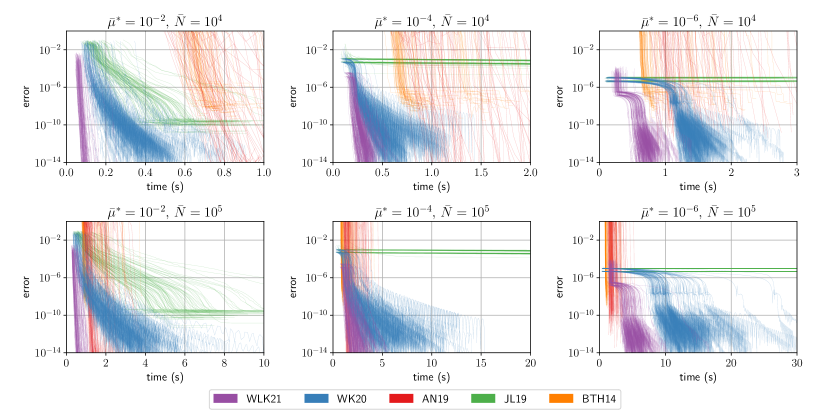
Figure 1: Comparison of algorithms for $n=10^{3}$.

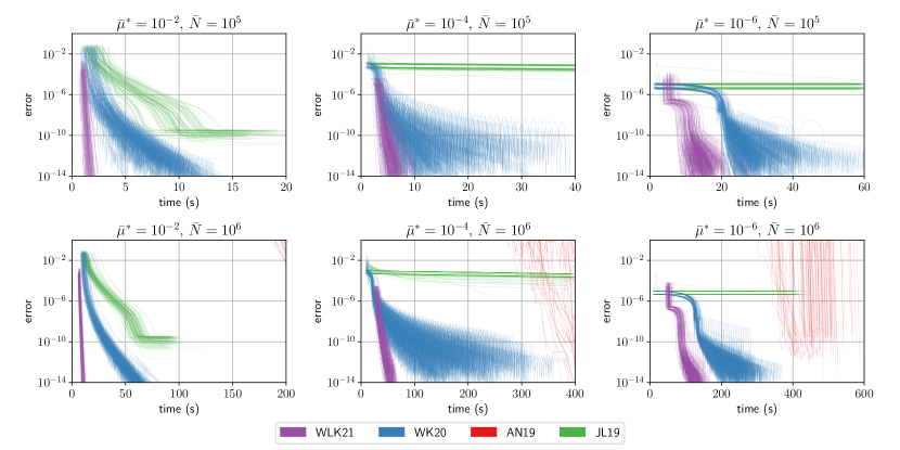
Figure 2: Comparison of algorithms for $n=10^{4}$.

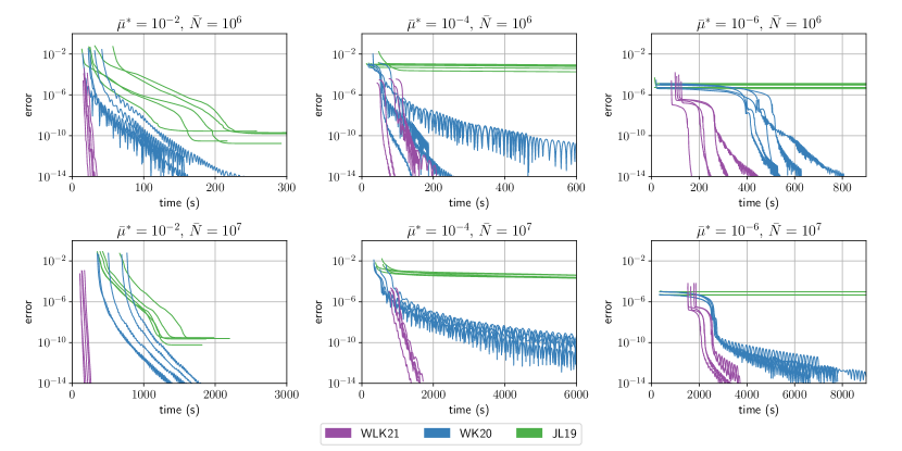
Figure 3: Comparison of algorithms for $n=10^{5}$.

• The lines plotted in Figures 1, 2 and 3 begin after time zero. For WLK21, WK20, and JL19 this gap corresponds to the time required to construct the corresponding convex reformulations of (1). For AN19, this corresponds to the time required to compute $x(\hat{\gamma})$ exactly, which is required to set up the appropriate $(2n+1)\times(2n+1)$ generalized eigenvalue problem [1]. For BTH14, this gap corresponds to the time required to compute a diagonalizing basis of (1).

• WLK21 constructs its reformulation faster than WK20 and JL19 when $\bar{\mu}^{*}=10^{-2}$. The situation is reversed for $\bar{\mu}^{*}\in\left\{10^{-4},10^{-6}\right\}$. Nevertheless, WLK21 outperforms both WK20 and JL19 due to its significantly improved performance in solving the resulting convex reformulation. See Appendix E.

• As expected from Theorem 1, WLK21 exhibits a linear convergence rate in terms of $\epsilon$. This is most apparent in the plots corresponding to $\bar{\mu}^{*}=10^{-2}$ and $\bar{\mu}^{*}=10^{-4}$.

• Although the convergence guarantees established for WK20 [34] and JL19 [19] do not depend on $\mu^{*}$, our results show empirically that these algorithms in fact perform better when $\mu^{*}$ is large. The degree to which the running times of these algorithms vary with $\mu^{*}$ is less than that of WLK21.

• The convergence rates of AN19 and BTH14 do not vary significantly with either $N$ or $\mu^{*}$, but they exhibit heavy dependence on $n$. Specifically, the convergence rate of AN19 empirically varies in $n$ as $\approx n^{2}$. This is consistent with the results reported in [1]. Similarly, due to the complete eigenbasis computation embedded in BTH14, we expect BTH14 to vary in $n$ as $\approx n^{3}$. Thus, as can be seen in Figures 1, 2 and 3, although AN19 outperforms WLK21 and WK20 for $(n,\bar{N},\bar{\mu}^{*})=(10^{3},10^{5},10^{-6})$, AN19 and BTH14 become impractical for $n=10^{4}$ and $n=10^{5}$.

• The saddle-point based first-order algorithm employed in JL19 is unable to decrease the error below $\approx 10^{-4}$ for $\bar{\mu}^{*}=10^{-4}$ and $\bar{\mu}^{*}=10^{-6}$.

Appendix A Useful lemmas regarding quadratic functions

The following two basic bounds will be useful in our error analysis.

Lemma 8.

Let $q(x)=x^{\top}Ax+2b^{\top}x+c$ for $A\in{\mathbb{S}}^{n}$, $b\in{\mathbb{R}}^{n}$, and $c\in{\mathbb{R}}$. Then, for all $x,y\in{\mathbb{R}}^{n}$, $\left\lvert q(x)-q(y)\right\rvert\leq\left\lVert A\right\rVert\left\lVert y-x\right\rVert^{2}+2\left(\left\lVert A\right\rVert\left\lVert x\right\rVert+\left\lVert b\right\rVert\right)\left\lVert y-x\right\rVert$. In particular, if $\left\lVert A\right\rVert,\left\lVert b\right\rVert\leq 1$, $\left\lVert x\right\rVert\leq\rho$ and $\left\lVert x-y\right\rVert\leq\delta$ for some $\delta\leq 1\leq\rho$, then $\left\lvert q(x)-q(y)\right\rvert\leq 5\delta\rho$.

Proof.

Writing $y=(y-x)+x$ and expanding the formula for $q(y)$, we obtain

$$q(y) =(y-x)^{\top}A(y-x)+2x^{\top}A(y-x)+x^{\top}Ax+2b^{\top}(y-x)+2b^{\top}x+c$$

$$=q(x)+\left((y-x)^{\top}A(y-x)+2\left\langle Ax+b,y-x\right\rangle\right).\qed$$

Lemma 9.

Let $\alpha,\beta,\gamma\in{\mathbb{R}}$ where $\alpha\neq 0$ and $\gamma/\alpha\leq 0$. Then the roots of $\alpha z^{2}+2\beta z+\gamma=0$ satisfy $\left\lvert z\right\rvert\leq 2\left\lvert\frac{\beta}{\alpha}\right\rvert+\sqrt{\frac{-\gamma}{\alpha}}$.

Proof.

Let $\left\{z_{-},z_{+}\right\}$ denote the roots (possibly with multiplicity). We bound

$$\left\{z_{-},\,z_{+}\right\} =\left\{-\tfrac{\beta}{\alpha}\pm\sqrt{\left(\tfrac{\beta}{\alpha}\right)^{2}-\tfrac{\gamma}{\alpha}}\right\}$$

$$\subseteq\left[-\tfrac{\beta}{\alpha}-\left(\left\lvert\tfrac{\beta}{\alpha}\right\rvert+\sqrt{\tfrac{-\gamma}{\alpha}}\right),\,-\tfrac{\beta}{\alpha}+\left(\left\lvert\tfrac{\beta}{\alpha}\right\rvert+\sqrt{\tfrac{-\gamma}{\alpha}}\right)\right]$$

$$\subseteq\left[-\left(2\left\lvert\tfrac{\beta}{\alpha}\right\rvert+\sqrt{\tfrac{-\gamma}{\alpha}}\right),\,\left(2\left\lvert\tfrac{\beta}{\alpha}\right\rvert+\sqrt{\tfrac{-\gamma}{\alpha}}\right)\right].\qed$$

Appendix B Useful procedures

This appendix contains running time guarantees for well-known algorithms that we will utilize as building blocks in Algorithm 1.

B.1 The Lanczos method

The following lemma characterizes the running time for approximating the minimum eigenvalue of a symmetric matrix.

Lemma 10 ([23]).

There exists an algorithm, $\textup{ApproxEig}(A,\rho,\delta,p)$, which given a symmetric matrix $A\in{\mathbb{S}}^{n}$, $\rho$ such that $\left\lVert A\right\rVert_{2}\leq\rho$, and parameters $\delta,p>0$, will, with probability at least $1-p$, return a unit vector $x\in{\mathbb{R}}^{n}$ such that $x^{\top}Ax\leq\lambda_{\min}(A)+\delta$. This algorithm runs in time

$$O\left(\tfrac{N\sqrt{\rho}}{\sqrt{\delta}}\log\left(\tfrac{n}{p}\right)\right),$$

where $N$ is the number of nonzero entries in $A$.

B.2 ApproxGamma

The following algorithm extends [34, Algorithm 2] to find a $\gamma\leq\hat{\gamma}$ such that $\mu(\gamma)$ falls in a prescribed range. An analogous algorithm can be used to find a $\gamma\geq\hat{\gamma}$ such that $\mu(\gamma)$ falls in a prescribed range.

Algorithm 5 ApproxGammaLeft

Given $(A_{0},A_{1})$, $(\xi,\zeta,\hat{\gamma})$, $p\in(0,1)$, and $\mu\in(0,\xi)$

1. Set $\ell_{1}=0$, $r_{1}=\hat{\gamma}$

2. For $t=1,\dots,T=\left\lceil\log\left(\tfrac{5\zeta}{\mu}\right)\right\rceil$

   1. $\gamma_{t}=(\ell_{t}+r_{t})/2$

   2. Let $x_{t}=ApproxEig\left(A(\gamma_{t}),2\zeta,\mu/8,p/T\right)$ and $\hat{\mu}_{t}=x_{t}^{\top}A(\gamma_{t})x_{t}$

   3. If $\hat{\mu}_{t}>\mu$, set $\ell_{t+1}=\ell_{t},\leavevmode\nobreak\ r_{t+1}=\gamma_{t}$

   4. Else if $\hat{\mu}_{t}<\tfrac{5}{8}\mu$, set $\ell_{t+1}=\gamma_{t},\leavevmode\nobreak\ r_{t+1}=r_{t}$

   5. Else, output $\gamma_{t}$, $x_{t}$

See 4

Proof.

We condition on ApproxEig succeeding in each call. This happens with probability at least $1-p$.

Suppose ApproxGammaLeft outputs on iteration $t$. On this iteration, we have $\mu(\gamma_{t})\geq\hat{\mu}_{t}-\mu/8\geq\mu/2$. Similarly note $x^{\top}A(\gamma_{t})x=\hat{\mu}_{t}\leq\mu$.

Next, we show that ApproxGammaLeft is guaranteed to output within $T$ iterations. Suppose otherwise and consider the interval

$${\cal I}\coloneqq\left\{\gamma\in{\mathbb{R}}_{+}:\,\begin{array}[]{l}\gamma\leq\hat{\gamma}\\ \mu(\gamma)\in\left[\tfrac{5}{8}\mu,\tfrac{7}{8}\mu\right]\end{array}\right\}.$$

Note that if $\gamma_{t}\in{\cal I}$ for some $t$ then ApproxGammaLeft will output at step $t$. Indeed, at iteration $t$, we will have $\hat{\mu}_{t}\in\left[\mu(\gamma_{t}),\mu(\gamma_{t})+\tfrac{\mu}{8}\right]\subseteq\left[\tfrac{5}{8}\mu,\mu\right]$. In particular, we deduce that $\gamma_{t}\notin{\cal I}$ for any $t=1,\dots,T$. Next, by construction, the interval $[\ell_{t},r_{t}]$ contains ${\cal I}$ for every $t$. On the other hand, $\left\lvert[\ell_{T},r_{T}]\right\rvert\leq 2^{-T}\zeta<\tfrac{\mu}{4}\leq\left\lvert{\cal I}\right\rvert$, a contradiction.

It remains to bound the running time of ApproxGammaLeft. By Lemma 10, each iteration of step 2.(b) runs in time

$$\tilde{O}\left(\tfrac{N\sqrt{\zeta}}{\sqrt{\mu}}\log\left(\tfrac{n}{p}\right)\right).$$

Finally, note that the number of iterations of step 2 is bounded by $T=O\left(\log\left(\tfrac{\zeta}{\mu}\right)\right)$. ∎

B.3 Conjugate gradient

The following lemma characterizes the running time for approximately minimizing a strongly convex quadratic function using the conjugate gradient algorithm.

Lemma 11.

There exists an algorithm, $\textup{ConjGrad}(A,b,\rho,\mu,\delta)$, which given symmetric matrix $A\in{\mathbb{S}}^{n}$ with $\mu I\preceq A\preceq\rho I$ and $b\in{\mathbb{R}}^{n}$, returns $x\in{\mathbb{R}}^{n}$ such that $\left\lVert x+A^{-1}b\right\rVert\leq\delta$. This algorithm runs in time

$$O\left(\tfrac{N\sqrt{\rho}}{\sqrt{\mu}}\log\left(\tfrac{\left\lVert b\right\rVert}{\mu\delta}\right)\right).$$

B.4 ApproxNu

The following algorithm uses the conjugate gradient algorithm to approximate $\nu(\gamma)$ for a given value of $\gamma$.

Algorithm 6 ApproxNu

Given $(A_{0},A_{1},b_{0},c_{0},c_{1})$, $(\xi,\zeta,\hat{\gamma})$ satisfying Assumption 2, $\gamma,\mu$ such that $\mu\in(0,1)$ and $A(\gamma)\succeq\mu I$, and $\delta>0$

• Apply the conjugate gradient method to find $\tilde{x}$ such that $\left\lVert\tilde{x}-x(\gamma)\right\rVert\leq\tfrac{\mu\delta}{10\zeta}$

• Return $\tilde{x}$, $q_{1}(\tilde{x})$

See 5

Proof.

The running time follows from Lemma 11. Note that Assumption 2 and $A(\gamma)\succeq\mu I$ together imply $\left\lVert x(\gamma)\right\rVert\leq\tfrac{2\zeta}{\mu}$. Then, from the definition of $\nu(\gamma)$ and $x(\gamma)$ and applying Lemma 8, we arrive at

$$\left\lvert q_{1}(\hat{x})-\nu(\gamma)\right\rvert \leq 5\left(\tfrac{2\zeta}{\mu}\right)\left(\tfrac{\mu\delta}{10\zeta}\right)\leq\delta.\qed$$

B.5 Nesterov’s accelerated minimax scheme

The following lemma characterizes the running time for finding an approximate optimizer of the maximum of two strongly convex smooth quadratic functions.

Lemma 12.

There exists an algorithm, AccMinimax, which given $A^{(1)},A^{(2)}\in{\mathbb{S}}^{n}$, $b^{(1)},b^{(2)}\in{\mathbb{R}}^{n}$, $c^{(1)},c^{(2)}\in{\mathbb{R}}$, and $(\mu,\rho,\delta)>0$ satisfying $\mu I\preceq A^{(i)}\preceq\rho I$ and $\left\lVert b^{(i)}\right\rVert\leq\rho$, will return $\bar{x}$ such that

$$\max_{i}\,\bar{x}^{\top}A^{(i)}\bar{x}+2b^{(i)\top}\bar{x}+c_{i}\leq\left(\min_{x\in{\mathbb{R}}^{n}}\max_{i}\,x^{\top}A^{(i)}x+2b^{(i)\top}x+c_{i}\right)+\delta,$$

in time

$$O\left(\tfrac{N\sqrt{\rho}}{\sqrt{\mu}}\log\left(\tfrac{\rho}{\delta\mu}\right)\right).$$

Proof.

For notational convenience, define $q^{(i)}(x)\coloneqq x^{\top}A^{(i)}x+2b^{(i)\top}x+c^{(i)}$ and $f(x)\coloneqq\max_{i}q^{(i)}(x)$. We may take $x_{0}=0$ in [27, Algorithm 2.3.12] and bound

$$f(0)-\min_{x}f(x) \leq f(0)-\max_{i}\min_{x}q^{(i)}(x)$$

$$\leq\max_{i}\left(q^{(i)}(0)-\min_{x}q^{(i)}(x)\right)$$

$$=\max_{i}\,b^{(i)\top}\left(A^{(i)}\right)^{-1}b^{(i)}$$

$$\leq\tfrac{\rho^{2}}{\mu}.$$

The running time then follows from [27, Theorem 2.3.5] and [34, Lemma 14]. ∎

Appendix C Deferred proofs from Section 2

Lemma 13.

Suppose Assumption 1 holds. Then

$$\operatorname{Opt}=\inf_{x\in{\mathbb{R}}^{n}}\sup_{\gamma\in\Gamma}q(\gamma,x).$$

Proof.

($\geq$) Let $x\in{\mathbb{R}}^{n}$ such that $q_{1}(x)\leq 0$. Then, as $\Gamma\subseteq{\mathbb{R}}_{+}$, we have $q_{0}(x)\geq\sup_{\gamma\in\Gamma}q(\gamma,x)$. Taking the infimum in $x$ concludes this direction.

($\leq$) Let $x\in{\mathbb{R}}^{n}$. We split into three cases depending on the sign of $q_{1}(x)$.

If $q_{1}(x)=0$, then $\operatorname{Opt}\leq q_{0}(x)=\sup_{\gamma\in\Gamma}q(\gamma,x)$.

Next, suppose $q_{1}(x)<0$ so that $\sup_{\gamma\in\Gamma}q(\gamma,x)=q(\gamma_{-},x)$. If $\gamma_{-}=0$, then again $\operatorname{Opt}\leq q_{0}(x)=\sup_{\gamma\in\Gamma}q(\gamma,x)$. On the other hand, if $\gamma_{-}>0$, then $A(\gamma_{-})\not\succeq 0$ and there exists nonzero $v\in\ker(A(\gamma_{-}))$. Without loss of generality, $\left\langle v,b(\gamma_{-})\right\rangle\leq 0$. Let $\alpha>0$ such that $q_{1}(x+\alpha v)=0$ (this exists as $v^{\top}A_{1}v=v^{\top}\frac{A(\bar{\gamma})-A(\gamma_{-})}{\bar{\gamma}-\gamma_{-}}v>0$). We deduce $\operatorname{Opt}\leq q_{0}(x+\alpha v)=q(\gamma_{-},x+\alpha v)\leq q(\gamma_{-},x)=\sup_{\gamma\in\Gamma}q(\gamma,x)$.

Finally, suppose $q_{1}(x)>0$. If $\Gamma$ is unbounded, then $\sup_{\gamma\in\Gamma}q(\gamma,x)=+\infty$ and $\operatorname{Opt}\leq\sup_{\gamma\in\Gamma}q(\gamma,x)$. Else, we have that $A(\gamma_{+})\not\succeq 0$ and there exists nonzero $v\in\ker(A(\gamma_{+}))$. An argument identical to the one in the previous paragraph shows $\operatorname{Opt}\leq\sup_{\gamma\in\Gamma}q(\gamma,x)$.

Taking the infimum over all $x\in{\mathbb{R}}^{n}$ completes the proof. ∎

Appendix D Deferred proofs from Section 4.1

In this appendix, we motivate a generalized-eigenvalue-based replacement for ApproxGammaLeft (Algorithm 5) of CRLeft (Algorithm 2). Given $\mu\in(0,\xi)$, our goal is to compute $\gamma\leq\hat{\gamma}$ and $v$ such that $\mu/2\leq\mu(\gamma)\leq v^{\top}A(\gamma)v\leq\mu$. We will do so by approximating the minimum eigenvalue $\tilde{\lambda}$ (and a corresponding eigenvector) for

$$-A_{1}v=\lambda\left(A(\hat{\gamma})-\tfrac{3\mu}{4}I\right)v$$ (6)

and setting $\tilde{\gamma}\coloneqq\hat{\gamma}+\tfrac{1}{\tilde{\lambda}}$. Note that defining $\gamma\coloneqq\hat{\gamma}+\tfrac{1}{\lambda}$, where $\lambda$ is the true minimum eigenvalue to (6), gives

$$\mu(\gamma) =\lambda_{\min}\left(A(\hat{\gamma})-\tfrac{3\mu}{4}I+\tfrac{1}{\lambda}A_{1}\right)+3\mu/4=3\mu/4.$$

In the following, we abbreviate $\hat{A}\coloneqq A(\hat{\gamma})-\tfrac{3\mu}{4}I$. As in Lemma 4, we will assume Assumption 2 throughout this appendix. We will take $\tilde{\lambda},\tilde{v}$ to be the output of eigifp on the input $(-A_{1},\hat{A},\delta)$ where $\delta>0$ will be fixed later.

Recall [12] that $\tilde{\lambda},\tilde{v}$ satisfies

$$(-A_{1}+B)\tilde{v}=\tilde{\lambda}(\hat{A}+C)\tilde{v}$$ (7)

for some $\left\lVert B\right\rVert\leq\delta\left\lVert A_{1}\right\rVert$ and $\left\lVert C\right\rVert\leq\delta\left\lVert\hat{A}\right\rVert$. We will assume that $\tilde{\lambda}$ is in fact the minimum eigenvalue of (7).

Lemma 14.

Suppose $\left\lvert\lambda-\tilde{\lambda}\right\rvert\leq\mu/5\zeta^{2}$, then $\mu(\tilde{\gamma})\geq\mu/2$.

Proof.

As $\mu(\tilde{\gamma})$ is $1$-Lipschitz, it suffices to show that $\left\lvert\tilde{\gamma}-\gamma\right\rvert\leq\mu/4$. Note that $\frac{1}{\lambda}=\gamma-\hat{\gamma}$ so that $\left\lvert\lambda\right\rvert\geq 1/\zeta$. We deduce that $\left\lvert\tilde{\lambda}\right\rvert\geq\left\lvert\lambda\right\rvert-\left\lvert\lambda-\tilde{\lambda}\right\rvert$. Combining,

$$\left\lvert\tilde{\gamma}-\gamma\right\rvert =\frac{\left\lvert\lambda-\tilde{\lambda}\right\rvert}{\left\lvert\lambda\right\rvert\left\lvert\tilde{\lambda}\right\rvert}\leq\frac{\tfrac{\mu}{5\zeta^{2}}}{\left(\tfrac{1}{\zeta}\right)\left(\tfrac{1}{\zeta}-\tfrac{\mu}{5\zeta^{2}}\right)}\leq\mu/4.\qed$$

Lemma 15.

Suppose $\tilde{\lambda}$ is a minimum eigenvalue of (7) and $2\delta\zeta\leq\xi/8$. Then,

$$\left\lvert\lambda-\tilde{\lambda}\right\rvert\leq\delta\tfrac{72\zeta}{\xi^{2}}.$$

Proof.

Note that

$$\lambda =\max\left\{\lambda:\,-A_{1}-\lambda\hat{A}\succeq 0\right\},\quad\text{and}\quad\tilde{\lambda}=\max\left\{\tilde{\lambda}:\,(-A_{1}+B)-\tilde{\lambda}(\hat{A}+C)\succeq 0\right\}.$$

We compute

$$-A_{1}-(\tilde{\lambda}-\alpha)\hat{A} =(-A_{1}+B)-\tilde{\lambda}(\hat{A}+C)-B+\tilde{\lambda}C+\alpha\hat{A}$$

$$\succeq-\delta(1+2\zeta|\tilde{\lambda}|)+\alpha\hat{A}.$$

We may thus deduce that $-A_{1}-(\tilde{\lambda}-\alpha)\hat{A}\succeq 0$ whenever $\alpha\geq\delta\frac{4(1+2\zeta|\tilde{\lambda}|)}{\xi}$. Hence,

$$\tilde{\lambda}-\lambda\leq\delta\frac{4(1+2\zeta|\tilde{\lambda}|)}{\xi}.$$

Similarly,

$$(-A_{1}+B)-(\lambda-\alpha)(\hat{A}+C) =-A_{1}-\lambda\hat{A}+B-\lambda C+\alpha(\hat{A}+C)$$

$$\succeq-\delta(1+2\zeta\left\lvert\lambda\right\rvert)+\alpha(\hat{A}+C).$$

We may thus deduce that $(-A_{1}+B)-(\lambda-\alpha)(\hat{A}+C)\succeq 0$ whenever $\alpha\geq\delta\frac{8(1+2\zeta\left\lvert\lambda\right\rvert)}{\xi}$. Hence,

$$\tilde{\lambda}-\lambda\geq-\delta\frac{8(1+2\zeta\left\lvert\lambda\right\rvert)}{\xi}.$$

Finally, we may estimate $\left\lvert\tfrac{1}{\lambda}\right\rvert\geq\tfrac{\xi}{4}$ and $\left\lvert\tfrac{1}{\tilde{\lambda}}\right\rvert\geq\tfrac{2\xi}{17}$. We conclude

$$-\delta\frac{8(1+8\zeta/\xi)}{\xi} \leq\tilde{\lambda}-\lambda\leq\delta\frac{4(1+17\zeta/\xi)}{\xi}.\qed$$

Proposition 5.

Let $\delta=\tfrac{\mu\xi^{2}}{360\zeta^{3}}$ and suppose $\tilde{\lambda}$ is the minimum eigenvalue of (7). Then,

$$\mu/2\leq\mu(\tilde{\gamma})\leq\tilde{v}^{\top}A(\tilde{\gamma})\tilde{v}\leq\mu.$$

Proof.

The first inequality follows from Lemmas 14 and 15. The second inequality follows from the definition of $\mu$. The third inequality follows as

$$\tilde{v}^{\top}A(\tilde{\gamma})\tilde{v} =\tilde{v}^{\top}\left(\hat{A}+\tfrac{1}{\tilde{\lambda}}A_{1}\right)\tilde{v}+3\mu/4$$

$$=\tilde{v}^{\top}\left((\hat{A}+C)+\tfrac{1}{\tilde{\lambda}}(A_{1}-B)-C+\tfrac{1}{\tilde{\lambda}}B\right)\tilde{v}+3\mu/4$$

$$\leq\left\lVert C\right\rVert+\tfrac{1}{|\tilde{\lambda}|}\left\lVert B\right\rVert+3\mu/4$$

$$\leq 4\delta\zeta+3\mu/4.$$

Here, the first inequality holds as $(-A_{1}+B)\tilde{v}=\tilde{\lambda}(\hat{A}+C)\tilde{v}$. The second inequality follows as $\left\lVert C\right\rVert\leq 2\delta\zeta$ and $\left\lvert\tilde{\lambda}\right\rvert\geq\left\lvert\lambda\right\rvert-\left\lvert\lambda-\tilde{\lambda}\right\rvert\geq 1/2\zeta$. ∎

Appendix E Numerical Experiment Tables

We provide additional statistics for the numerical results plotted in Figures 1, 2 and 3 for $n=10^{3},\,10^{4},\,10^{5}$, respectively. In Tables 1 and 2, we present the averages for $n=10^{3},\,10^{4}$ respectively over 100 random instances each, and in Table 3 the averages for $n=10^{5}$ are given over 5 random instances. In these tables, Error and ErrorCR correspond to the error of $q_{0}(\tilde{x})$ and the error of $\bar{x}$ within the convex reformulation respectively as defined in Section 4.3. For WLK21, WK20 and JL19, we also report time for constructing the convex reformulation and solving the reformulation as Ref. and Solve. For each parameter combination, we highlight the algorithm with the smallest running time.

		$\bar{N}=10^{4}$					$\bar{N}=10^{5}$
					Time					Time
$\bar{\mu}^{*}$	Alg.	Error	ErrorCR	Time	Ref.	Solve	Error	ErrorCR	Time	Ref.	Solve
	WLK21	4.8	6.1	0.1	0.05	0.05	5.1	5.4	0.8	0.3	0.4
	WK20	5.7	6.7	0.5	0.1	0.3	4.8	5.3	4.4	0.5	3.8
1e-2	JL19	1.5e+03	1.8e+06	0.7	0.1	0.6	5.1e+01	2.1e+06	8.2	0.6	7.6
	AN19	6.7e+02	-	1.5	-	-	6.4e+02	-	2.2	-	-
	BTH14	4.2e+08	-	1.1	-	-	7.5e+08	-	1.5	-	-
	WLK21	6.7	7.2	0.4	0.2	0.2	8.5	8.4	2.9	1.0	1.8
	WK20	8.1	7.1	0.7	0.1	0.6	7.0	7.1	7.0	0.6	6.4
1e-4	JL19	2.3e+09	4.1e+12	3.0	0.1	2.8	1.0e+09	3.6e+12	49.9	0.6	49.3
	AN19	4.9	-	1.6	-	-	5.0	-	2.4	-	-
	BTH14	4.0e+08	-	1.2	-	-	4.4e+08	-	1.7	-	-
	WLK21	6.5	6.1	0.8	0.3	0.5	8.3	8.2	6.3	1.8	4.4
	WK20	6.4	6.4	1.6	0.1	1.5	7.6	8.2	15.5	0.5	15.0
1e-6	JL19	7.9e+04	7.5e+10	3.1	0.1	3.0	8.4e+04	7.1e+10	40.4	0.5	39.9
	AN19	1.4e+06	-	1.7	-	-	1.3e+06	-	2.4	-	-
	BTH14	1.3e+09	-	1.4	-	-	1.0e+09	-	1.7	-	-

Table 1: Average errors and solution times for $n=10^{3}$ over 100 random instances for each parameter combination. Note that errors are reported in units of $10^{-16}$. We call attention to the setting $(\bar{N},\bar{\mu}^{*})=(10^{5},10^{-6})$. In this setting, the fastest algorithm is BTH14. On the other hand, BTH14 also reports the highest error of $\approx 10^{-7}$. BTH14 is followed by AN19 which achieves slightly smaller error of $\approx 10^{-10}$. While WLK21 is slightly slower than both of these algorithms it achieves significantly smaller errors of $\approx 10^{-16}$. The results are similar for $(\bar{N},\bar{\mu}^{*})=(10^{5},10^{-4})$ as well.

		$\bar{N}=10^{4}$					$\bar{N}=10^{5}$
					Time					Time
$\bar{\mu}^{*}$	Alg.	Error	ErrorCR	Time	Ref.	Solve	Error	ErrorCR	Time	Ref.	Solve
	WLK21	4.9	6.4	1.8	0.8	0.9	4.7	5.4	11.1	4.8	4.8
	WK20	4.9	5.7	9.8	1.6	8.1	5.3	6.0	67.5	10.5	56.8
1e-2	JL19	1.4e+02	1.7e+06	15.3	1.6	13.6	6.3e+02	1.8e+06	93.8	10.7	82.8
	AN19	6.8e+02	-	184.1	-	-	1.2e+03	-	324.5	-	-
	WLK21	1.5e+01	1.6e+01	6.6	2.6	3.7	4.1e+01	4.2e+01	57.0	24.0	30.3
	WK20	1.0e+01	1.1e+01	16.6	1.5	15.1	2.9e+01	3.0e+01	207.0	11.0	195.8
1e-4	JL19	6.7e+09	4.2e+12	57.9	1.5	56.4	2.1e+10	3.1e+12	393.1	11.3	381.6
	AN19	4.3	-	205.7	-	-	4.5	-	476.4	-	-
	WLK21	9.1e+01	9.2e+01	15.1	5.1	9.8	2.7e+01	2.8e+01	130.7	49.1	79.0
	WK20	6.1e+01	6.1e+01	33.0	1.5	31.5	3.1e+01	3.1e+01	264.0	10.6	253.2
1e-6	JL19	2.5e+09	7.8e+10	59.7	1.5	58.1	1.6e+08	7.1e+10	402.7	11.0	391.4
	AN19	8.0e+06	-	206.6	-	-	4.4e+06	-	475.5	-	-

Table 2: Average errors and solution times for $n=10^{4}$ over 100 random instances for each parameter combination. Note that errors are reported in units of $10^{-16}$.

		$\bar{N}=10^{4}$					$\bar{N}=10^{5}$
					Time					Time
$\bar{\mu}^{*}$	Alg.	Error	ErrorCR	Time	Ref.	Solve	Error	ErrorCR	Time	Ref.	Solve
	WLK21	3.3	9.9	30.1	12.6	13.6	5.3	2.7	229.2	100.8	101.7
1e-2	WK20	4.7	7.8	162.9	24.7	137.0	3.1	4.9	1748.4	527.9	1216.3
	JL19	4.9	1.4e+06	287.3	27.4	259.1	1.6e+02	2.3e+06	1930.7	419.0	1507.5
	WLK21	1.5e+01	1.6e+01	141.6	65.1	70.8	9.5e+01	9.5e+01	1586.3	767.0	728.5
1e-4	WK20	1.6e+01	1.6e+01	334.3	25.7	307.9	1.4e+02	1.4e+02	10622.9	437.7	10180.8
	JL19	2.5e+09	4.3e+12	1044.3	26.8	1016.5	9.2e+10	8.7e+11	11526.9	514.5	11007.9
	WLK21	2.2e+01	2.0e+01	294.2	97.8	190.0	6.2e+01	6.4e+01	3361.1	1569.5	1701.7
1e-6	WK20	1.5e+01	1.6e+01	612.3	25.7	585.6	1.4e+02	1.4e+02	7781.5	367.8	7409.8
	JL19	7.6e+04	8.5e+10	1081.4	19.5	1061.2	2.1e+06	7.5e+10	10960.0	355.3	10600.8

Table 3: Average errors and solution times for $n=10^{5}$ over 5 random instances for each parameter combination. Note that errors are reported in units of $10^{-16}$.

References

- Adachi and Nakatsukasa [2019] S. Adachi and Y. Nakatsukasa. Eigenvalue-based algorithm and analysis for nonconvex QCQP with one constraint. Math. Program., 173:79–116, 2019.
- Ben-Tal and den Hertog [2014] A. Ben-Tal and D. den Hertog. Hidden conic quadratic representation of some nonconvex quadratic optimization problems. Math. Program., 143:1–29, 2014.
- Ben-Tal and Nemirovski [2001] A. Ben-Tal and A. Nemirovski. Lectures on Modern Convex Optimization, volume 2 of MPS-SIAM Ser. Optim. SIAM, 2001.
- Ben-Tal and Teboulle [1996] A. Ben-Tal and M. Teboulle. Hidden convexity in some nonconvex quadratically constrained quadratic programming. Math. Program., 72:51–63, 1996.
- Carmon and Duchi [2018] Y. Carmon and J. C. Duchi. Analysis of Krylov subspace solutions of regularized nonconvex quadratic problems. arXiv preprint, 1806.09222, 2018.
- Conn et al. [2000] A. R. Conn, N. I. Gould, and P. L. Toint. Trust Region Methods, volume 1 of MPS-SIAM Ser. Optim. SIAM, 2000.
- Ekeland and Temam [1999] I. Ekeland and R. Temam. Convex Analysis and Variational Problems, volume 28 of Classics Appl. Math. SIAM, 1999.
- Fallahi et al. [2018] S. Fallahi, M. Salahi, and T. Terlaky. Minimizing an indefinite quadratic function subject to a single indefinite quadratic constraint. Optimization, 67(1):55–65, 2018.
- Feng et al. [2012] J.M. Feng, G.X. Xuan, R.L. Sheu, and Y. Xia. Duality and solutions for quadratic programming over single non-homogeneous quadratic constraint. J. Global Optim., 54(2):275–293, 2012.
- Fortin and Wolkowicz [2004] C. Fortin and H. Wolkowicz. The Trust Region Subproblem and semidefinite programming. Optim. Methods and Softw., 19(1):41–67, 2004.
- Fradkov and Yakubovich [1979] A. L. Fradkov and V. A. Yakubovich. The S-procedure and duality relations in nonconvex problems of quadratic programming. Vestnik Leningrad Univ. Math., 6:101–109, 1979.
- Golub and Ye [2002] G. H. Golub and Q. Ye. An inverse free preconditioned krylov subspace method for symmetric generalized eigenvalue problems. SIAM Journal on Scientific Computing, 24(1):312–334, 2002.
- Gould et al. [1999] N. I. M. Gould, S. Lucidi, M. Roma, and P. L. Toint. Solving the Trust-Region Subproblem using the Lanczos method. SIAM J. Optim., 9(2):504–525, 1999.
- Hazan and Koren [2016] E. Hazan and T. Koren. A linear-time algorithm for trust region problems. Math. Program., 158:363–381, 2016.
- Hmam [2010] H. Hmam. Quadratic optimisation with one quadratic equality constraint. Technical report, Defence Science and Technology Organisation Edinburgh (Australia) Electronic Warfare and Radar Division, 2010.
- Ho-Nguyen and Kılınç-Karzan [2017] N. Ho-Nguyen and F. Kılınç-Karzan. A second-order cone based approach for solving the Trust Region Subproblem and its variants. SIAM J. Optim., 27(3):1485–1512, 2017.
- Huang and Sidiropoulos [2016] K. Huang and N. D. Sidiropoulos. Consensus-ADMM for general quadratically constrained quadratic programming. IEEE Transactions on Signal Processing, 64(20):5297–5310, 2016.
- Jiang and Li [2016] R. Jiang and D. Li. Simultaneous diagonalization of matrices and its applications in quadratically constrained quadratic programming. SIAM J. Optim., 26(3):1649–1668, 2016.
- Jiang and Li [2019] R. Jiang and D. Li. Novel reformulations and efficient algorithms for the Generalized Trust Region Subproblem. SIAM J. Optim., 29(2):1603–1633, 2019.
- Jiang and Li [2020] R. Jiang and D. Li. A linear-time algorithm for generalized trust region problems. SIAM J. Optim., 30(1):915–932, 2020.
- Jiang et al. [2018] R. Jiang, D. Li, and B. Wu. SOCP reformulation for the Generalized Trust Region Subproblem via a canonical form of two symmetric matrices. Math. Program., 169:531–563, 2018.
- Karmarkar et al. [1991] N. Karmarkar, M. G. Resende, and K. G. Ramakrishnan. An interior point algorithm to solve computationally difficult set covering problems. Math. Program., 52:597–618, 1991.
- Kuczynski and Wozniakowski [1992] J. Kuczynski and H. Wozniakowski. Estimating the largest eigenvalue by the power and Lanczos algorithms with a random start. SIAM J. Matrix Anal. Appl., 13(4):1094–1122, 1992.
- Locatelli [2015] M. Locatelli. Some results for quadratic problems with one or two quadratic constraints. Oper. Res. Lett., 43(2):126–131, 2015.
- Moré [1993] J. J. Moré. Generalizations of the trust region problem. Optim. methods and Softw., 2(3-4):189–209, 1993.
- Moré and Sorensen [1983] J. J. Moré and D. C. Sorensen. Computing a trust region step. SIAM J. on Sci. and Stat. Comput., 4(3):553–572, 1983.
- Nesterov [2018] Y. Nesterov. Lectures on convex optimization. Number 137 in Springer Optim. and its Appl. Springer, 2 edition, 2018.
- Pardalos et al. [1991] P. M. Pardalos, Y. Ye, and CG Han. Algorithms for the solution of quadratic knapsack problems. Linear Algebra Appl., 152:69–91, 1991.
- Pólik and Terlaky [2007] I. Pólik and T. Terlaky. A survey of the S-lemma. SIAM Rev., 49(3):371–418, 2007.
- Pong and Wolkowicz [2014] T.K. Pong and H. Wolkowicz. The generalized trust region subproblem. Computational Optimization and Applications, 58(2):273–322, 2014.
- Salahi and Fallahi [2016] M. Salahi and S. Fallahi. Trust region subproblem with an additional linear inequality constraint. Optim. Lett., 10(4):821–832, 2016.
- Stern and Wolkowicz [1995] R. J. Stern and H. Wolkowicz. Indefinite trust region subproblems and nonsymmetric eigenvalue perturbations. SIAM J. Optim., 5(2):286–313, 1995.
- Wang and Jiang [2021] A. L. Wang and R. Jiang. New notions of simultaneous diagonalizability of quadratic forms with applications to QCQPs. arXiv preprint, 2101.12141, 2021.
- Wang and Kılınç-Karzan [2020] A. L. Wang and F. Kılınç-Karzan. The generalized trust region subproblem: solution complexity and convex hull results. Math. Program., 2020. doi: 10.1007/s10107-020-01560-8. Forthcoming.