nuSQuIDS: A toolbox for neutrino propagation

Abstract

The Neutrino Simple Quantum Integro-Differential Solver (nuSQuIDS) is a C++ code based on SQuIDS that propagates an ensemble of neutrinos through given media. Neutrino oscillation calculations relevant to current and next-generation experiments are implemented. This includes coherent and non-coherent neutrino interactions in settings such as the Sun, Earth, or a vacuum. The code is designed to be accurate and flexible, while at the same time maintaining good performance. It has a modular design that allows the user to incorporate new physics in novel scenarios.

figuresection

1 Introduction

In recent decades a large body of evidence that neutrinos change flavor as they propagate macroscopic distances due to the non-alignment of their mass and flavor eigenstates has accumulated from solar [1, 2], atmospheric [3, 4, 5, 6], accelerator [7, 8, 9, 10], and reactor [11, 12, 13] experiments. Thanks to these remarkable experimental results and related theoretical calculations, the neutrino-mass-induced flavor oscillation paradigm [14, 15, 16, 17, 18, 19, 20, 21] has been firmly established and the three mixing angles, which parametrize the lepton-mixing matrix, together with the two squared-mass differences, have been measured to good precision [22, 23, 24, 25]. It is the task of on-going and future experiments to determine the neutrino-mass ordering and the $CP$-violating phase [26, 27, 28, 29, 30]. Also, the IceCube Neutrino Observatory has recently made precise measurements of the atmospheric spectrum above 100 GeV, where the Earth is no longer transparent to neutrinos [31, 32, 33], allowing new physics models to be constrained [34, 35]. The identification of high-energy extraterrestrial neutrinos [34, 36, 37] has opened the possibility of exploring new physics at these energies as well [38, 39, 40, 41, 42].

Matter effects play a fundamental role in the explanation of solar neutrinos [43, 44], which has motivated the study of new flavor-changing neutrino interactions [45, 46, 47, 48, 49, 50, 51, 52]. Even though most data can be explained in the standard three neutrino framework, some puzzling anomalies still remain  [53, 54, 55, 56, 57, 58, 59, 60, 61]. These may be explained by introducing new light neutrino states [62, 63, 64, 65, 61, 66, 67] and other new physics  [68, 69, 70, 71, 72, 73, 74, 75, 76, 77, 78, 79, 80, 81, 82, 83, 84]. Also, the interplay between cosmology and neutrino oscillation has been widely studied in the literature  [85, 86, 87, 88, 89, 90, 91]. Generally, neutrinos are good probes to perform fundamental physics tests [26, 92, 93, 94].

Tools are needed to compute neutrino propagation accurately and reliably. In classical computations, where the only effect of propagation is neutrino oscillation, libraries such as GLoBES  [95], Prob3++ [96, 97], and nuCRAFT [98] are available; for a recent comparison of oscillation calculations comparisons see [99]. On quantum computers, such as the IBM-Q systems, implementations using two entangled qubits have also been developed [100]. Unfortunately, when non-coherent interactions [101, 102, 103, 104] are important, these methods are no longer applicable. In the high-energy regime, when oscillations can be neglected, tools have been developed to propagate neutrinos taking into account non-coherent interactions; for example, TauRunner [105], NuPropEarth [106], nuFATE [107], JuLiET [108, 109], among others [110, 111]. Beyond these general-purpose codes, packages have also been developed to propagate tau neutrinos specifically, e.g. NuTAuSim [112] and nuPyProp [113]. However, none of the above-mentioned packages are able to take coherent and non-coherent neutrino interactions into account simultaneously. Furthermore, the ability to allow the user to incorporate new physics models or to change the propagation medium is also limited in some of these packages. nuSQuIDS seeks to address all of these limitations by providing a highly-customizable package while at the same time remaining numerically efficient.

In section 2 we review neutrino oscillation and interaction theory, in section 3 we summarize the main features of the code, in section 4 we show the use of the code in a few representative scenarios, in section 5 we discuss how this code compares to other software, in section 6 we show the performance of the library, and finally section 7 presents concluding remarks.

Additionally, an extended appendix that provides further useful information about the code. In E we describe the unit tests that are provided with the library, in B we describe the main classes and structure of the code; and finally, in C we describe the library Python interface.

2 Mathematical Framework

2.1 Neutrino Oscillations

In this section we briefly review neutrino oscillations using the density matrix formalism. We can represent the state of a neutrino ensemble at an energy $E$ and position $x$ using the density matrix. In the weak-interaction flavor-eigenstate basis, $\{\left|\nu_{\alpha}\right\rangle\}$, it can be written as

$$\rho(E,x)=\sum_{\alpha}\phi_{\alpha}(E,x)\left|\nu_{\alpha}\right\rangle\left\langle\nu_{\alpha}\right|,$$ (1)

where $\phi_{\alpha}$ specifies the flux of flavor $\alpha$. These eigenstates can be related with the mass eigenstates, $\{\left|\nu_{i}\right\rangle\}$, by

$$\left|\nu_{\alpha}\right\rangle=\sum_{i}U^{*}_{\alpha i}\left|\nu_{i}\right\rangle,$$ (2)

where $U$ is a unitary matrix known as the Pontecorvo-Maki-Nakagawa-Sakata (PMNS) matrix, or neutral lepton mixing matrix. For antineutrinos, the relation is the same as in Eq. (2) with $U\to U^{*}$. It is customary to parametrize $U$ as a product of complex rotations,

$$U(\theta_{ij}\delta_{ij})=R_{N-1\,N}R_{N-2\,N}...R_{45}R_{35}R_{25}R_{15}R_{34}R_{24}R_{14}R_{23}R_{13}R_{12},$$ (3)

determined by angles, $\{\theta_{ij}\}$, and phases, $\{\delta_{ij}\}$ [114, 115]; see [116] for a recent discussion about parameterizations of the PMNS matrix. When considering the standard three-flavor paradigm, the following parametrization is often used:

$$U=\begin{pmatrix}c_{12}c_{13}&s_{12}c_{13}&s_{13}e^{-i\delta_{13}}\\ -s_{12}c_{23}-c_{12}s_{23}s_{13}e^{i\delta_{13}}&c_{12}c_{23}-s_{12}s_{23}s_{13}e^{i\delta_{13}}&s_{23}c_{13}\\ s_{12}s_{23}-c_{12}c_{23}s_{13}e^{i\delta_{13}}&-c_{12}s_{23}-s_{12}c_{23}s_{13}e^{i\delta_{13}}&c_{23}c_{13}\end{pmatrix}\,,$$ (4)

where $c_{ij}\equiv\cos\theta_{ij}$, $s_{ij}\equiv\sin\theta_{ij}$. In the three-flavor scenario, we use this parametrization (with values from [22] by default). The neutrino ensemble propagation is described by the following quantum Von Neumann equation

$$\frac{\partial\rho(E,x)}{\partial x}=-i[H(E,x),\rho(E,x)].$$ (5)

In general, the Hamiltonian, $H$, can always be split into time-dependent and time-independent parts. For neutrino oscillations, the following splitting is convenient:

$$H(E,x)=H_{0}(E)+H_{1}(E,x),$$ (6)

with

$$H_{0}(E) =\frac{1}{2E}{\rm diag}(0,\Delta m^{2}_{21},\Delta m^{2}_{31},\Delta m^{2}_{41},...,\Delta m^{2}_{n1}),$$ (7a)

$$H_{1}(E,x) =\sqrt{2}G_{F}U^{\dagger}{\rm diag}(N_{e}(x)-N_{nuc}(x)/2,-N_{nuc}(x)/2,-N_{nuc}(x)/2,0,...,0)U,$$ (7b)

where $n$ is the number of neutrino states, $G_{F}$ is the Fermi constant, $N_{e}(x)$ and $N_{nuc}(x)$ are the electron and nucleon number densities at position $x$, and $\Delta m^{2}_{i1}$ are the neutrino mass square differences. In writing these equations, we have used the convention that the first three flavor eigenstates correspond to $\nu_{e}$, $\nu_{\mu}$, and $\nu_{\tau}$ respectively, while the rest are assumed to be sterile neutrinos. $H_{0}$ arises from the neutrino kinetic term, whereas $H_{1}$ incorporates the matter potential induced by coherent forward scattering [117, 118, 119]. Note that the matter potential, $H_{1}$, given in Eq. (7b) for neutrinos changes to $-H_{1}^{*}$ for antineutrinos. Since the propagation due to $H_{0}$ can be solved analytically, it is convenient to use the so-called interaction picture. For an operator $O(x)$ the interaction picture transformed operator, $O_{I}(x)$ is defined as

$$O_{I}(x)=\exp(-iH_{0}x)O(x)\exp(iH_{0}x).$$ (8)

The corresponding evolution equation for the neutrino state is

$$\frac{\partial\rho_{I}(E,x)}{\partial x}=-i[H_{1I}(E,x),\rho_{I}(E,x)]~{}.$$ (9)

2.2 Non-coherent Interactions

So far, we have only incorporated vacuum oscillations and matter effects through coherent interactions, but we now wish to extend this formalism to incorporate non-coherent interactions and collective neutrino behavior. In what follows, we will remove the subindex $I$ and assume that all operators, unless specified, are in the interaction picture. This problem has been extensively discussed in the literature, [120, 121, 122, 123, 124, 125, 126], for specificity we follow the formalism and notation given in [127]. The neutrino (antineutrino), $\rho$ $(\bar{\rho})$, kinetic equations are

$$\frac{\partial\rho(E,x)}{\partial x} = -i[H_{1}(E,x),\rho(E,x)]-\left\{\Gamma(E,x),\rho(E,x)\right\}+F\left[\rho,\bar{\rho};E,x\right],$$ (10a)

$$\frac{\partial\bar{\rho}(E,x)}{\partial x} = i[H^{*}_{1}(E,x),\bar{\rho}(E,x)]-\left\{\bar{\Gamma}(E,x),\rho(E,x)\right\}+\bar{F}\left[\rho,\bar{\rho};E,x\right],$$ (10b)

where $\Gamma$ and $\bar{\Gamma}$ are functions that incorporate the effect of attenuation due to non-coherent interactions, and $F$ and $\bar{F}$ are functionals on $\rho$ and $\bar{\rho}$ that take into account interactions between different energies for neutrinos and antineutrinos.

In nuSQuIDS, the attenuation terms are

$$\Gamma(E,x) = \frac{1}{2}\sum_{\alpha}\frac{\Pi_{\alpha}(E,x)}{\lambda^{\alpha}_{\rm NC}(E,x)+\lambda^{\alpha}_{\rm CC}(E,x)},$$ (11a)

$$\bar{\Gamma}(E,x) = \frac{1}{2}\sum_{\alpha}\frac{\bar{\Pi}_{\alpha}(E,x)}{\bar{\lambda}^{\alpha}_{\rm NC}(E,x)+\bar{\lambda}^{\alpha}_{\rm CC}(E,x)+\bar{\lambda}^{\alpha}_{\rm GR}(E,x)},$$ (11b)

where $\Pi_{\alpha}(E,x)$ is the neutrino projector onto flavor $\alpha\in\{e,\mu,\tau\}$, $\lambda^{\alpha}_{\rm CC}$ ($\lambda^{\alpha}_{\rm NC}$) is the charged (neutral) current neutrino interaction length, given by $(N_{nuc}(x)\sigma^{\alpha}_{\rm CC(NC)}(E))^{-1}$[101, 102, 103, 104, 128], and $\bar{\lambda}^{e}_{\rm GR}$ is the mean free path due to the Glashow resonance $(N_{e}(x)\sigma^{e}_{\rm GR}(E))^{-1}$ [102]. Notice that we assume the matter only contains electrons, protons, and neutrons, i.e. $\bar{\lambda}^{\mu}_{\rm GR}=\bar{\lambda}^{\tau}_{\rm GR}=0$. The other interaction terms are as follows:

$$F\left[\rho,\bar{\rho};E,x\right] = \sum_{\alpha}\Pi_{\alpha}(E,x)\int_{E}^{\infty}{\rm Tr}\left[\Pi_{\alpha}(E_{\nu_{\alpha}},x)\rho(E_{\nu_{\alpha}},x)\right]\frac{1}{\lambda^{\alpha}_{\rm NC}(E_{\nu_{\alpha}},x)}\frac{\partial N^{\alpha}_{\rm NC}(E_{\nu_{\alpha}},E)}{\partial E}dE_{\nu_{\alpha}}$$ (12a)

$$+\Pi_{\tau}(E,x)\int_{E}^{\infty}\int_{E_{\tau}}^{\infty}{\rm Tr}\left[\Pi_{\tau}(E_{\nu_{\tau}},x)\rho(E_{\nu_{\tau}},x)\right]$$

$$\hskip 56.9055pt\times\frac{1}{\lambda^{\tau}_{\rm CC}(E_{\nu_{\tau}},x)}\frac{\partial N^{\tau}_{\rm CC}(E_{\nu_{\tau}},E_{\tau})}{\partial E_{\tau}}\frac{\partial N^{\rm all}_{\rm dec}(E_{\tau},E)}{\partial E}dE_{\nu_{\tau}}dE_{\tau}$$

$$+\Big{(}{\rm Br}_{e}\Pi_{e}(E,x)+{\rm Br}_{\mu}\Pi_{\mu}(E,x)\Big{)}\int_{E}^{\infty}\int_{E_{\tau}}^{\infty}{\rm Tr}\left[\bar{\Pi}_{\tau}(E_{\bar{\nu}_{\tau}},x)\bar{\rho}(E_{\bar{\nu}_{\tau}},x)\right]$$

$$\hskip 56.9055pt\times\frac{1}{\bar{\lambda}^{\tau}_{\rm CC}(E_{\bar{\nu}_{\tau}},x)}\frac{\partial\bar{N}^{\tau}_{\rm CC}(E_{\bar{\nu}_{\tau}},E_{\tau})}{\partial E_{\tau}}\frac{\partial\bar{N}^{\rm lep}_{\rm dec}(E_{\tau},E)}{\partial E}dE_{\bar{\nu}_{\tau}}dE_{\tau}$$

$$\bar{F}\left[\rho,\bar{\rho};E,x\right] = \sum_{\alpha}\bar{\Pi}_{\alpha}(E,x)\int_{E}^{\infty}{\rm Tr}\left[\bar{\Pi}_{\alpha}(E_{\bar{\nu}_{\alpha}},x)\bar{\rho}(E_{\bar{\nu}_{\alpha}},x)\right]\frac{1}{\bar{\lambda}^{\alpha}_{\rm NC}(E_{\bar{\nu}_{\alpha}},x)}\frac{\partial\bar{N}^{\alpha}_{\rm NC}(E_{\bar{\nu}_{\alpha}},E)}{\partial E}dE_{\bar{\nu}_{\alpha}}$$

$$+\bar{\Pi}_{\tau}(E,x)\int_{E}^{\infty}\int_{E_{\tau}}^{\infty}{\rm Tr}\left[\bar{\Pi}_{\tau}(E_{\bar{\nu}_{\tau}},x)\bar{\rho}(E_{\bar{\nu}_{\tau}},x)\right]$$

$$\hskip 56.9055pt\times\frac{1}{\bar{\lambda}^{\tau}_{\rm CC}(E_{\nu_{\tau}},x)}\frac{\partial\bar{N}^{\tau}_{\rm CC}(E_{\bar{\nu}_{\tau}},E_{\tau})}{\partial E_{\tau}}\frac{\partial\bar{N}^{\rm all}_{\rm dec}(E_{\tau},E)}{\partial E}dE_{\bar{\nu}_{\tau}}dE_{\tau}$$

$$+\Big{(}{\rm Br}_{e}\bar{\Pi}_{e}(E,x)+{\rm Br}_{\mu}\bar{\Pi}_{\mu}(E,x)\Big{)}\int_{E}^{\infty}\int_{E_{\tau}}^{\infty}{\rm Tr}\left[\Pi_{\tau}(E_{\nu_{\tau}},x)\rho(E_{\nu_{\tau}},x)\right]$$

$$\hskip 56.9055pt\times\frac{1}{\lambda^{\tau}_{\rm CC}(E_{\nu_{\tau}},x)}\frac{\partial N^{\tau}_{\rm CC}(E_{\nu_{\tau}},E_{\tau})}{\partial E_{\tau}}\frac{\partial N^{\rm lep}_{\rm dec}(E_{\tau},E)}{\partial E}dE_{\nu_{\tau}}dE_{\tau}$$

$$+\left(\sum_{\alpha}\bar{\Pi}_{\alpha}(E,x)\right)\int_{E}^{\infty}{\rm Tr}\left[\bar{\Pi}(E_{\bar{\nu}_{e}},x)\bar{\rho}(E_{\bar{\nu}_{e}},x)\right]\frac{1}{\bar{\lambda}_{\rm GR}(E_{\bar{\nu}_{e}},x)}\frac{\partial\bar{N}^{e}_{\rm GR}(E_{\bar{\nu}_{e}},E)}{\partial E}dE_{\bar{\nu}_{e}}$$

where ${\rm Br}_{\alpha}$ is the $\tau$ branching ratio to $\nu_{\alpha}$,

$$\frac{\partial N^{\alpha}_{\rm CC(NC)}(E_{\nu_{\alpha}},E_{\alpha})}{\partial E_{\alpha}} = \frac{1}{\sigma^{\alpha}_{\rm CC(NC)}(E_{\nu_{\alpha}})}\frac{\partial\sigma^{\alpha}_{\rm CC(NC)}(E_{\nu_{\alpha}},E_{\alpha})}{\partial E_{\alpha}},$$ (13a)

$$\frac{\partial\bar{N}^{e}_{\rm GR}(E_{\bar{\nu}_{e}},E_{e})}{\partial E_{e}} = \frac{1}{\bar{\sigma}^{e}_{\rm GR}(E_{\bar{\nu}_{e}})}\frac{\partial\bar{\sigma}^{e}_{\rm GR}(E_{\bar{\nu}_{e}},E_{e})}{\partial E_{e}},$$ (13b)

are the charged-current, neutral-current, and Glashow resonance interaction. The $\tau$ decay distribution [129] in all modes and leptonic modes are

$$\frac{\partial N^{\rm lep}_{\rm dec}(E_{\tau},E)}{\partial E} = \frac{1}{{\tilde{\Gamma}_{\rm lep}}^{\tau}(E_{\tau})}\frac{\partial\tilde{\Gamma}_{\rm lep}^{\tau}(E_{\tau},E)}{\partial E},$$ (14)

$$\frac{\partial N^{\rm all}_{\rm dec}(E_{\tau},E)}{\partial E} = \frac{1}{{\tilde{\Gamma}_{\rm all}}^{\tau}(E_{\tau})}\frac{\partial\tilde{\Gamma}_{\rm all}^{\tau}(E_{\tau},E)}{\partial E},$$ (15)

where $\tilde{\Gamma}^{\tau}(E_{\tau})=\frac{E_{\tau}}{m_{\tau}}\tau_{\tau}$, in which $m_{\tau}$ is the $\tau$ mass and $\tau_{\tau}$ is the $\tau$ lifetime, “all” and “lep” indicate the all and leptonic $\tau$ decay modes, respectively.

The first term in Eqs. (12a) and (12) accounts for neutrino re-injection at lower energies coming from Eqs. (11a) and (11b) due to neutral-current interaction. The second and third term is the injection due to the $\tau$ decay into $\nu_{\tau}$ and into other flavors in the leptonic case: this is known as tau-regeneration. It is important to note that the latter terms couple the propagation of neutrinos and antineutrinos. Finally, the last term in Eq. (12) accounts for the neutrinos produced in the Glashow resonance due to $W^{-}$ decay.

These equations are implemented by discretizing the problem in bins that the user specifies. The user should be aware that the discretization used can introduce errors due to bin spill-over. Special care should be taken for hard spectra, e.g. $\phi(E_{\nu})=E^{-1}$, where this maybe more relevant and the user is encouraged to check the effect of discretization by modifying the energy nodes spacing and cross sections’ granularity.

3 Features

3.1 Standard oscillations in matter and vacuum

nuSQuIDS is able to compute the neutrino oscillation probabilities in the presence of matter. Neutrino oscillations can be computed for up to six neutrino flavors out of the box, though this can be extended to an arbitrary number of neutrino flavors by producing additional tables using the provided Mathematica files. The calculation allows setting both the mixing angles and the $CP$-violating phases. Using the Body and Track objects, nuSQuIDS can compute the oscillation probability in any media provided by the user. Default media, such as the Earth, the Sun, a constant density slab, and others are provided for immediate use. In general, no constraints exist in the trajectory of the neutrino oscillation, though in the provided implementations, all neutrinos are assumed to travel in straight lines, which should cover most applications.

Though some of this functionality is available in other neutrino oscillation calculators [95, 96, 97, 98], the solution implemented in nuSQuIDS is unique, and provides advantages over others. By working in the neutrino interaction basis, the fast oscillations due the the vacuum part of the neutrino Hamiltonian are solved analytically. This provides significant speed up in propagating neutrinos in dense environments, specially for slowly-changing or small matter densities. An unusual feature of nuSQuIDS is that it solves the neutrino oscillation problem over a grid of energies; though solving the problem (when considering only coherent effects) using an individual, fixed neutrino energy is also possible, as in other software. In the multi-energy operating mode, nuSQuIDS can interpolate the interaction-picture solutions of the neutrino-evolution problem for energy values that are in between the nodes where the calculation is performed. This allows accurate and fast evaluation of the neutrino oscillation probability using a relatively coarse grid. This is particularly important when evaluating the neutrino oscillation probability over a larger number of energies, which is often the case when re-weighting large Monte Carlo data sets.

3.2 Extendability to new physics scenarios

nuSQuIDS implements the standard neutrino oscillation Hamiltonian with matter effects; however, this can be extended to include additional terms that may appear in the Hamiltonian. This can be achieved as illustrated in example 4.2, where the user creates an inherited class of the main nuSQuIDS class and implements the desired new physics operators. In order to write the operators, the user needs to write in terms of the SQuIDS SU(N) vector type, which represents arbitrary hermitian matrices. Additionally, SQuIDS implements operations between matrices and scalars that typically arise in writing these terms, e.g. matrix-scalar multiplication, commutator between matrices, etc. Once the new Hamiltonian is defined by the user no further change is needed. The user will be able to use all the functionality of nuSQuIDS with the new physics. Finally, nuSQuIDS allows for the serialization of user-defined values which allow for constants used by new physics operators to be serialized as part of nuSQuIDS serialization.

3.3 Neutrino transport in dense media

nuSQuIDS implements non-coherent neutrino interactions that are relevant in very dense media or when neutrinos have high energies. This functionality is comparable to other neutrino propagators used in neutrino telescopes [105, 106, 107, 108, 109, 110, 111, 112, 113]. At high energies, the neutrino interaction length is comparable to the size of the Earth, making the neutrino transport non-trivial. nuSQuIDS takes into account charged-current and neutral-current interactions with nucleons through deep-inelastic scattering, which is the dominant interaction at the relevant energies [101, 102, 103, 104, 128]. Additionally, it takes into account neutrino-electron scattering, which is only relevant for resonant electron-antineutrino scattering at neutrino energies close to 6.4 PeV [130]. A subdominant contribution from neutrino-photon scattering is not implemented [131, 132, 133, 103, 104], but can be easily extended in our framework; see [106] for a publicly-available implementation of this cross section. Finally, the production of neutrinos from lepton decay is neglected for all flavors, except for tau neutrinos. In this case, we account for the contribution of neutrinos from tau decay in the approximation that the tau decays promptly, so it does not undergo significant energy losses. This approximation is good below approximately 10 PeV and breaks down at higher energies; see [105, 106, 113] for recent work on implementing tau neutrino propagation at very high energies.

3.4 Scenarios with neutrino oscillations and interactions

nuSQuIDS is able to take into account simultaneously the presence of oscillations and non-coherent interactions in a consistent manner. For neutrino transport in the Earth, and when standard neutrino oscillations are considered, this scenario is never an issue, since oscillations are important only below $\sim 100$ GeV, while interactions appear above $\sim 10$ TeV. However, this is not the case for neutrino transport in larger astrophysical objects, e.g. high-energy neutrinos produced in cosmic-ray collisions [134, 135, 136, 137, 138, 139, 140, 141] or produced from dark matter decay or annihilation [142, 143, 144, 125, 145, 146] in the Sun undergo oscillations and interactions simultaneously. Additionally, this is not the case for non-standard neutrino oscillations, notably for light sterile neutrinos motivated by short-baseline anomalies, where flavor conversion can happen at high energies where interactions are relevant [147, 148, 149, 150, 151, 152, 153, 154, 155, 156, 157].

3.5 Handling of extended sources

Neutrino emission does not happen as a physical point source, but rather there exist finite emission regions. However, since the neutrino oscillation and interaction scales are much larger than the production region or detector size, in most scenarios, we can consider the neutrino emission to be point like to good approximation. Nonetheless, there are scenarios where this approximation is not applicable. For example, for neutrinos produced from dark matter decay through an intermediate mediator, a scenario known as secluded dark matter [158], the neutrinos are produced according to an exponential distribution that can be as large as the radius of the Earth or Sun depending on the model parameters [159, 146]. This scenario can be implemented in nuSQuIDS [146] by introducing a source term that follows the exponential yield of neutrinos. Another relevant scenario is that of production of neutrinos in pion or kaon decay in flight, e.g. in accelerator neutrino experiments or in cosmic-ray air-showers. Though for standard neutrino oscillation parameters the distribution of lengths induced by the varying decay position does not significantly impact the oscillation probability, this is not the case for new physics models that introduce small oscillations scales, e.g. when heavier neutrinos are introduced. A similar scenario is that of experiments looking for fast oscillations close to cores of nuclear reactors where the size of the core is relevant.

3.6 Efficient fast oscillations and fully delocalized neutrino emission

Neutrino oscillations can vary extremely rapidly with neutrino energy, especially at small energies where the neutrino Hamiltonian in vacuum is large. It is numerically expensive to solve the neutrino evolution on a very dense grid or for enough energies to be able to produce a meaningful oscillation pattern. nuSQuIDS introduces a novel solution to this problem by permitting the evaluation of fast oscillations in a way that the oscillations due to vacuum are tracked analytically. The evaluation of oscillations on a grid of nodes that has been already computed has been significantly optimized making it possible to evaluate the oscillation probability for large Monte Carlo data sets much faster than computing the individual oscillation probabilities at each of the Monte Carlo event energies.

As noted in the previous point, the issue of fast oscillations and the localization of the neutrino emission is related. Neutrinos emitted by an extended source smear out the neutrino oscillation probability statistically. nuSQuIDS provides an option to analytically perform the smearing of the oscillation probability, in which the user provides the size of the oscillation length that they which to smear. This can be understood as the leading order of the Magnus expansion [160], and can speed up numerical calculations dramatically in some concrete physics setups, such as oscillations in the early universe [88]. This calculation has no significant overhead and is much more efficient than performing integrals over the production region. This feature is most useful in computing the oscillation expected from a nuclear reactor on a nearby detector, where one typically needs to smear over the reactor core size, or in computing the yield of atmospheric neutrino oscillations where one needs to smear over the production region in the atmosphere, which is several kilometers in size.

3.7 Serializable input and output

nuSQuIDS allows for the result of a calculation to be serialized into an HDF5 file. The serialization stores all the settings that were used to produce the nuSQuIDS object. This can be advantageous in several scenarios. For example, a calculation can be complex and lengthy, and the user may choose to perform it in steps. In this scenario, the user can stop the calculation at a given point and then recover the nuSQuIDS object where it was left and continue. Another scenario of interest is that related to not knowing at execution time which energies will need to be computed. In this case, the user performs a calculation on a grid of energies and then stores the output of nuSQuIDS in a file. Then, later, when the user wants to evaluate the result at specific energies, they can recover the object and perform the necessary evaluations. This is also useful when the same calculation will be reused many times.

3.8 Techniques for high-performance Monte Carlo evaluation

nuSQuIDS separates the calculation of a result flux from an input flux at the user’s selected energy nodes from evaluating that result flux at arbitrary energies (provided those energies are within the span of energy nodes for which the propagation was performed). As discussed previously, this latter step evaluates vacuum oscillations analytically, and interpolates all other effects between the nearest energy nodes. As the final flux evaluation is often desired for very large numbers of energies (e.g. for every event produced in a Monte-Carlo simulation), it has been optimized for speed, and furthermore to permit concurrent evaluation. While the majority of the classes and functions in nuSQuIDS are not safe to access concurrently from multiple threads of execution, such use is specifically supported for all for the flux evaluation functions. While not applicable in all cases, concurrent evaluation may provide considerable speed improvements for some users.

3.9 C++ and Python interfaces

nuSQuIDS has been written in C++ since this compiled language provides the best execution efficiency. Extensive use is made internally of templating, inlining, and auto-vectorization to produce efficient machine code. In particular, the algebra of SU(N) operators significantly benefits from these types of optimization. All nuSQuIDS functions can be accessed in C++; however, recently, there has been great interest in designing particle physics software in interpreted languages such as Python. To facilitate the usage of nuSQuIDS with Python-based physics software, an interface to Python is implemented by means of the Boost library. Most of the functionality of nuSQuIDS is available through the Python interface, with the notable exception of new body objects and new physics operators. These limitations arise because these types of extensions require user-provided functions which must be evaluated very frequently during the propagation calculation, which, if written in Python, would produce a significant amount of overhead.

4 Usage Examples

Provided along with the code are a set of working examples demonstrating its use for various purposes. Here, we discuss two illustrative use cases: computing neutrino oscillations for a range of energies simultaneously, and extending the base implementation in the library with new physics.

4.1 Multiple Energy Propagation

In this section, we discuss an abbreviated version of the multiple energy propagation example found in the examples/Multiple_energy subdirectory.

Unit conversion factors and physical constants are provided by the supporting SQuIDS library’s Const class. It is typical to allocate an instance of this class to make these conveniently available:

⬇

1squids::Const units;

Next, we construct the nuSQUIDS object itself. For the multiple-energy mode, it requires an array of energies for which calculations will be carried out, which we choose here to be 200 values, spaced logarithmically from 1 GeV to 1,000 GeV. We choose the number of neutrino flavors to consider to be four: three active flavors and one sterile. These inputs are passed to the class constructor, along with the neutrino constant for the third argument to indicate that we will consider only neutrinos and not anti-neutrinos, and false for the fourth argument to disable the calculation of non-coherent interactions.

⬇

1auto energies = logspace(1.*units.GeV, 1.e4*units.GeV, 200);

2unsigned int numneu = 4;

3nuSQUIDS nus(energies, numneu, neutrino, false /*no interactions*/);

Next, we choose the environment (matter profile) through which we will propagate the neutrino flux. We choose here the Earth, with path passing through its full diameter, and apply these choices to the nuSQUIDS object:

⬇

1double phi = units.pi; // zenith angle for trajectory

2auto earth_atm = std::make_shared<EarthAtm>();

3auto track_atm = std::make_shared<EarthAtm::Track>(earth_atm->MakeTrack(phi));

4nus.Set_Body(earth_atm);

5nus.Set_Track(track_atm);

A variety of other Body classes are provided with the library for media such as vacuum, constant density material, material with user-specified variable density, and the Sun. Additionally, users can create their own Body implementations for needs not covered by these. Each Body type has an associated Track class, parameterizing paths through it in whatever manner is most appropriate.

The parameters of the neutrino mixing matrix can be fully customized. Here, we take a set of nominal values:

⬇

3nus.Set_MixingAngle(0,1,0.563942);

4nus.Set_MixingAngle(0,2,0.154085);

5nus.Set_MixingAngle(1,2,0.785398);

6nus.Set_SquareMassDifference(1,7.65e-05);

7nus.Set_SquareMassDifference(2,0.00247);

8nus.Set_SquareMassDifference(3,0.1);

9nus.Set_MixingAngle(1,3,0.1);

Mixing angles are expressed in radians, and are labeled by the lower an upper states they connect, with zero-based indexing. Squared mass differences are specified in eV² and are always with respect to the lowest-mass eigenstate, so only the upper state index must be specified. $CP$-violating phases can also be specified, again in radians and with two state indices. If unspecified, they default to zero.

Next, the initial neutrino flux before propagation must be configured. Here, we will use a simple power-law spectrum, purely of the $\nu_{\mu}$ flavor (determined by the k == 1 condition). The flux is specified as a two-dimensional array, indexed by neutrino flavor and energy:

⬇

5marray<double,2> inistate{energies.size(), numneu};

6double N0 = 1.0e18;

7for(int i = 0 ; i < inistate.extent(0); i++){

8 for(int k = 0; k < inistate.extent(1); k ++){

9 inistate[i][k] = (k == 1) ? N0*pow(energies[i],-2) : 0.0;

10 }

11}

12nus.Set_initial_state(inistate,flavor);

If we choose to work with both neutrinos and anti-neutrinos at the same time, this array would be rank three, with an additional, middle index taking on values zero for neutrinos and one for anti-neutrinos.

A number of settings are exposed which govern how the ODE solving process operates. The most critical are the error tolerances, whose values should be chosen based on the precision needed and the difficulty of the propagation problem; see Sec 6.1 for more detailed discussion.

⬇

9nus.Set_rel_error(1.0e-5);

10nus.Set_abs_error(1.0e-5);

After all settings are configured, the propagation itself can be performed:

⬇

12nus.EvolveState();

At this point, the propagated flux can be examined. For simplicity, we evaluate it for all three flavors over a grid of energies, and write these results to a file, from which they can be plotted, etc.:

⬇

10std::ofstream file("fluxes_flavor.txt");

11file << "#␣E␣flux-nu_e␣flux-nu_mu␣flux-nu_tau\n";

12for(double E : logspace(1.*units.GeV, 1.e4*units.GeV, 1000)){

13 file << E << "␣";

14 for(int fl=0; fl<numneu; fl++)

15 file << "␣" << nus.EvalFlavor(fl, E);

16 file << "\n";

17}

It is worth noting that we can evaluate the final flux on a grid of energies much more dense that was used for the propagation. This takes advantage of the interpolation between propagated energies, which automatically includes vacuum oscillations, providing a more precise approximation than a physics-unaware interpolation. Fig. 1 shows the oscillation probabilities calculated in this example.

Figure 1: Output for the multiple-energy mode with oscillations including a sterile neutrino (3+1)

4.2 Extended Physics

Besides using the physics phenomena already implemented in nuSQuIDS, users can extend it with various forms of new physics. This is accomplished by writing a class derived from the provided nuSQUIDS class, and customizing one or more of the physics member functions used during evolution. These functions are H0–the time-independent portion of the Hamiltonian from Eq. 7, HI–the time-dependent portion of the Hamiltonian from Eq. 7, GammaRho–the function describing non-coherent attenuation of the neutrino state (combining $\Gamma$ and $\bar{\Gamma}$ from Eq. 10), InteractionsRho–the function describing additions to the neutrino state (combining $F$ and $\bar{F}$ from Eq. 10), GammaScalar–analogous to GammaRho for any scalar fields added to the system, InteractionsScalar–analogous to InteractionsRho for any scalar fields, and the helper AddToPreDerive which can be used for any time/position dependent bookkeeping in the implementation, although only a subset are likely to need customization for any particular physics scenario.

As an example of this, we demonstrate implementing a non-standard interaction (NSI). This requires defining the interaction as an operator using the squids::SU_vector type, and adding a contribution from it to the time-dependent Hamiltonian. First, we define the new class:

⬇

1class nuSQUIDSNSI: public nuSQUIDS {

2 private:

3 double epsilon_mutau;

4 squids::SU_vector NSI;

5 std::vector<squids::SU_vector> NSI_evol;

6

7 void AddToPreDerive(double x);

8 squids::SU_vector HI(unsigned int ei,unsigned int index_rho) const;

9

10 public:

11 nuSQUIDSNSI(double epsilon_mutau, marray<double,1> Erange,

12 int numneu, NeutrinoType NT,

13 bool iinteraction, double th01=0.563942,

14 double th02=0.154085, double th12=0.785398);

15};

We add three member variables: epsilon_mutau–the sole NSI parameter we will support, NSI–the operator we construct from it, and NSI_evol to hold time-evolved copies of NSI as an optimization. We will add a new implementation of HI to update the Hamiltonian, as well as using AddToPreDerive to pre-calculate updates to NSI_evol. A new constructor will take the value of the NSI parameter, as well as the standard oscillation angles, which influence the value of the NSI operator.

⬇

17nuSQUIDSNSI(double epsilon_mutau, marray<double,1> Erange,

18 int numneu, NeutrinoType NT, bool iinteraction,

19 double th01, double th02, double th12)

20 : nuSQUIDS(Erange,numneu,NT,iinteraction),

21 epsilon_mutau(epsilon_mutau)

22{

23 assert(numneu == 3);

24 // define the flavor structure as a complex matrix

25 gsl_matrix_complex* M = gsl_matrix_complex_calloc(3,3);

26 gsl_complex c {{ epsilon_mutau , 0.0 }};

27 gsl_matrix_complex_set(M,2,1,c);

28 gsl_matrix_complex_set(M,1,2,gsl_complex_conjugate(c));

29 NSI = squids::SU_vector(M);

30 gsl_matrix_complex_free(M);

31

32 Set_MixingAngle(0,1,th01);

33 Set_MixingAngle(0,2,th02);

34 Set_MixingAngle(1,2,th12);

35 // rotate to mass representation

36 NSI.RotateToB1(params);

37

38 NSI_evol.resize(ne);

39 for(int ei = 0; ei < ne; ei++)

40 NSI_evol[ei] = squids::SU_vector(nsun);

41}

The constructor creates the NSI operator in the flavor basis from a matrix representation, then transforms it to the mass basis for later use. Note that setting the mixing angles defines the effect of the RotateToB1 basis-transformation function. The NSI_evol vector is filled with a set of correctly-sized operator vectors, but their values are not yet computed. Due to the simplicity of the example, only three-neutrino scenarios are supported, with other settings being rejected.

The implementation of AddToPreDerive is responsible for computing the time-evolved operator values, which depend on both the time/position of the system–x and on the time-independent Hamiltonian for each energy, accessed from the base class’ H0_array:

⬇

15void AddToPreDerive(double x){

16 for(int ei = 0; ei < ne; ei++)

17 NSI_evol[ei] = NSI.Evolve(H0_array[ei],(x-Get_t_initial()));

18}

The implementation of HI can then make use of NSI_evol, knowing that AddToPreDerive will be called to update it for each x before any calls to HI are made.

The implementation of HI itself is concerned with adding the additional term to the Hamiltonian:

⬇

41squids::SU_vector HI(unsigned int ei,unsigned int index_rho) const{

42 static const double HI_prefactor=params.sqrt2*params.GF*params.Na*pow(params.cm,-3);

43 double CC = HI_prefactor*current_density*current_ye;

44 squids::SU_vector potential = (3.0*CC)*NSI_evol[ei];

45

46 if ((index_rho == 0 and NT==both) or NT==neutrino){

47 // neutrino potential

48 return nuSQUIDS::HI(ei,index_rho) + potential;

49 } else if ((index_rho == 1 and NT==both) or NT==antineutrino){

50 // antineutrino potential

51 return nuSQUIDS::HI(ei,index_rho) + -1*std::move(potential);

52 }

53 throw std::runtime_error("nuSQUIDS::HI␣:␣unknown␣particle␣or␣antiparticle");

54}

A few details to note are that current_density and current_ye are member variables of the nuSQUIDS class which are used to obtain the matter properties (density and electron fraction) at the current position, the base nuSQUIDS::HI is invoked to obtain the original, standard model terms of the Hamiltonian, and that when the potential term must have the opposite sign for the anti-neutrino case, we apply the std::move function to it before performing the multiplication by $-1$ to indicate that the object’s contents may be overwritten, eliminating the need for a temporary storage buffer.

The full implementation of the class contains several other useful and convenient features, such as updating the serialization mechanism to save and restore the additional physics parameter; for the details we refer the reader to the file examples/NSI/NSI.h in the code. With the nuSQUIDSNSI class fully defined, its usage is analogous to the original nuSQUIDS, with the only major difference being the extra parameters for the constructor; setting the initial state, running the evolution, and reading out the final state are the same.

While this example makes only a very simple addition to the physics of nuSQuIDS, there are a wide variety possibilities of equal of greater complexity, such as new non-coherent interactions and additional, coupled scalar fields.

5 Comparison to Other Software

A number of other software packages are available which perform related calculations. In this section, we summarize how a number of these differ from nuSQuIDS. Most neutrino propagation software can be divided into categories based on whether it was designed to handle neutrino oscillation physics or neutrino absorption physics. nuSQuIDS is unusual in this regard, as it is designed to calculate both types of effect simultaneously. Another important categorization is the calculation method used, which tends to have implications for the physics effects which can be readily calculated: Three prevalent methods, each with different strengths and weaknesses, are algebraic matrix diagonalization, ordinary differential equation (ODE) integration, and Monte-Carlo (MC) sampling. Matrix diagonalization is frequently used for coherent effects (e.g. neutrino oscillation) in uniform media, for which the system of differential equations can be written down and solved analytically, as introduced in [161]. This has the advantage of taking a small, constant time to solve, but loses efficiency when variations in the propagation medium must be approximated by repeating the calculation in many small steps, and is not normally applicable to physics effects which couple fluxes besides those of different flavors at the same energy (such as energy losses due to neural-current interactions). ODE integration, the method used by nuSQuIDS, consists of writing down all physics effects in terms of their differential effects on neutrino fluxes and numerically solving the resulting system of equations. This provides a quite natural framework for treating variable media and arbitrary coupling between fluxes, but requires care in discretizing the problem (e.g. in neutrino energy), in structuring the problem numerically for handling by a standard ODE integration routine, and in selecting the parameters of the integration routine to get precise results rapidly. Monte Carlo sampling is in some sense the more literal method, consisting of simulating individual particles and randomly sampling the interactions they undergo. This sampling has both the benefit and disadvantage that it discovers not only the average behavior but also the full distribution of variations from it. This is indispensable when the full distribution is required, but has relatively slow convergence to precisely extract the mean behavior if that is all that is sought. Monte Carlo sampling can not only naturally treat variable media, but requires no discretization.

Package	Method	Oscillation	Absorption	Variable Density
GLoBES	AD	✓
Prob3++	AD	✓
nuCraft	ODE	✓		✓
nuFATE	ODE		✓	✓
nuPropEarth	MC		✓	✓
TauRunner	MC		✓	✓
ANIS	MC		✓	✓
nuSQuIDS	ODE	✓	✓	✓

Table 1: Simple classification of neutrino evolution codes by calculation technique (analytic diagonalization–AD, differential equation integration–ODE, or Monte Carlo sampling–MC), whether they treat neutrino oscillation, absorption, or both, and whether they directly support propagation in variable density media.

The General Long Baseline Experiment Simulator (GLoBES) [95] is a toolkit to enable analyzing the capabilities of neutrino oscillation experiments, and combinations of experiments. Calculating neutrino flux evolutions is thus not the package’s primary purpose, but is nonetheless one of its key components. GLoBES calculates only oscillation effects, via the analytic diagonalization method. Via its add-on system, the package can treat new physics effects, including sterile neutrinos, with the snu add-on.

Prob3++ [96] is designed specifically to calculate neutrino oscillation probabilities for the Super-Kamiokande collaboration. As such, it calculates only oscillation effects, and only for up to three flavors, although Lorentz invariance-violating oscillations are also supported for searches for new physics. As the package uses the analytic diagonalization method, only constant-density media are directly supported, although to support atmospheric neutrino measurements, the full Earth may be approximated as a set of spherically concentric shells of material, with a distinct density and electron fraction for each shell.

nuCraft [98] is a package created specifically to facilitate searches for sterile neutrino effects in the atmospheric neutrino flux, so it focuses on the computation of oscillation effects with support for four or more neutrino flavors, and has a continuous treatment of the density profile of the Earth. Unlike the other pure oscillation calculators, nuCraft is an ODE integration-based system, which makes inclusion of the variable material density convenient.

Turning to packages designed for higher energies with a focus on neutrino absorption, the All Neutrino Interaction Simulation (ANIS) [162] is intended for use as an event generator for neutrino observatories. For this reason it uses a Monte-Carlo sampling approach, and not only simulates neutrinos passing through the bulk of the Earth, with a continuously-parameterized density profile, but also includes forcing final interactions in a volume defined as the vicinity of a detector. (This volume is typically larger than the instrumented volume of the detector in order to fully sample muons produced by charge-current $\nu_{\mu}$ interactions entering the detector from outside.) While ANIS treats all deep-inelastic scattering (DIS) and Glashow resonance (resonant $W^{\pm}$ production) processes as well as tau propagation and decay, it does not calculate oscillations. The code requires DIS cross sections in the somewhat unusual form of Bjorken x, y pairs, pre-sampled at natural frequencies from the desired cross section. While this enables the propagation code to run rapidly and without direct dependencies on other software, the user must beware that systematic biases will result if sufficiently large tables are not used.

nuPropEarth [163] is a newer package which is similar to ANIS, but adds treatment of a number of subdominant interaction processes, such as nuclear effects. It also uses a Monte-Carlo sampling method, and does not treat oscillations. Choosing different tradeoffs than ANIS, nuPropEarth links directly to the GENIE/HEDIS, TAUOLA++, and TAUSIC packages to enable the use of recent and highly detailed cross sections treatments, but with the disadvantage of a considerable set of dependencies required to build the package.

TauRunner [105] is a new Python package that provides similar functionality to nuPropEarth. It has the advantage that it has less dependence on other software, and allows for arbitrary media and trajectories. It also uses a Monte-Carlo sampling method, and does not treat oscillations. It can use several built-in cross-section tables that can be extended by the user. These tables only account for deep-inelastic scattering. More importantly, TauRunner properly accounts for the tau energy losses at very high energies, where the on-spot decay approximation used in nuSQuIDS breaks down.

Finally, nuFATE [164] is a tool for calculation of neutrino flux attenuations at high energies, which uses a particularly efficient differential equation solution method which avoids the need for using a general ODE-integration routine by applying an integrating factor transformation, so that only the material density profile must be integrated, rather than the coupled system of equations. While this mechanism does support deep inelastic scattering, the Glashow resonance, and tau-regeneration all in a continuously variable medium, in its current form the package does not support distinct cross sections for different target species, either at the level of individual nucleon types, or different nuclei.

6 Performance and Precision

In the tests described in this section, Machine 1 is configured with an Intel Core™ i7-6700K CPU, with a ‘base’ frequency of 4.0 GHz. All tests were performed with the ‘Turbo Boost’ feature disabled, preventing frequency scaling.

The time evolution and basis transformations performed on squids::SU_vector objects rely heavily on trigonometric functions, specifically sines and cosines, mostly in matched pairs. These operations are in turn used by several of the key portions of nuSQuIDs, and for oscillation-only calculations evaluation of trigonometric functions can be the single largest part of time consumed by the library. As a result, runtime is significantly dependent on the performance of the underlying math library, which is usually supplied by the operating system, or sometimes the compiler. The differences are illustrated in Table 2, which shows measurements performed on Machine 1 with several combinations of operating system and compiler of the cost of computing a single sine function or the combination of sine and cosine for the same argument (which should ideally be performed by an efficient, fused calculation). A measurement was also made of the time to run the pseudo-random number generator (PRNG) by itself. The time spent for the PRNG varies somewhat, assumedly due to different optimization choices by the various compilers, but amounts to a small fraction of the time for the trigonometric calculation. Broadly, it is apparent that the calculations using the math implementations from the older version of the GNU C library (glibc) are significantly slower than the versions using other math libraries. The (approximately) factor of two difference in fused sine/cosine performance between glibc 2.17 and 2.28 translates into a 10-25% difference in the overall runtime of nuSQuIDs oscillation calculations. The user is therefore cautioned that the choice of compiler and runtime libraries can be important to maximizing the performance of nuSQuIDs. The benchmarks shown in this section will use the GNU compiler, version 8.3.1 (Red Hat 8.3.1-5) on CentOS 8, as this is a combination with good performance which is likely to be relevant to many users.

OS	Compiler	PRNG	Sine	Sine & Cosine	Math Library
CentOS 7	gcc 4.8.5	6.0 ns	40.5 ns	63.5 ns	GNU C Library 2.17
CentOS 7	gcc 7.3.1	2.7 ns	37.1 ns	63.3 ns	GNU C Library 2.17
CentOS 7	clang 5.0.1	4.8 ns	96.4 ns	69.0 ns	GNU C Library 2.17
CentOS 7	icc 18.0.3	4.0 ns	20.9 ns	22.2 ns	libimf 2018.3.222
CentOS 8	gcc 8.3.1	2.7 ns	26.8 ns	31.3 ns	GNU C Library 2.28
Darwin 16.7.0	clang 5.0.0	2.9 ns	19.1 ns	20.1 ns	libsystem_m 3121.6.0
FreeBSD 11.2	clang 6.0.1	2.9 ns	22.3 ns	30.8 ns	BSD libc

Table 2: Measured time to compute trigonometric functions using different compilers and operating systems on Machine 1. In each case, the same stream of $10^{8}$ pseudo-random arguments in the domain [-100,100] was used, and the average time per call was computed, including the time necessary for the PRNG to compute the next argument value.

6.1 Parameters Affecting Precision

The primary quantity defining the size of the problem solved by nuSQuIDS in its multiple energy mode is the number of energy nodes included in the calculation. It is important to note that the interpolation provided by nuSQuIDS allows arbitrary energies within the range of the energy nodes to be evaluated after propagating, so it is not necessary to calculate a node for every energy at which the final flux may be needed. Rather, the minimum number of nodes should be chosen so that the calculation is suitably precise at each node and when interpolated between nodes.

It is difficult to give specific guidance for all of the many types of problems to which nuSQuIDs is applied, so users are advised to be prepared to perform their own tests of how many nodes are needed to get good results for their use cases. However, it can be noted that for most problems the authors have attempted to compute numbers of nodes in the range 100-300 have typically been found sufficient. It is also important that, while it is often convenient to place nodes uniformly in energy or the logarithm of energy, this is by no means required by nuSQuIDS, so it can be advantageous to place nodes more densely in regions of particular interest or where sharp spectral features are expected, such as the vicinity of the Glashow resonance.

A second key parameter is the requested error tolerance for the ODE integration, which effectively controls the number of steps the integrator must take, while the number of energy nodes causes the amount of work required to compute each step to vary. As with the number of nodes, it is impossible to give one-size-fits-all advice on selecting the tolerance. In general, problems which include greater variation in the magnitudes of the flux values at different energies (e.g. steep power law fluxes), or for different flavors, require more demanding tolerances in order for the small components to be computed precisely in the presence of the larger components. Similar to selecting the number of energy nodes, the necessary tolerance may be found by incrementally tightening it until subsequent calculations produce results which are equivalent to within the desired precision. While this process is manual and somewhat annoying, having been performed for one problem, the result can usually be applied to modified versions of the problem without retesting, as long as the changes are not drastic.

Listing 1: A simple routine for comparing the precision of two different calculations with nuSQuIDS. Error checking, that numbers of energy ranges, number of flavors, etc. are compatible is advisable, but omitted here for brevity.

⬇

void compare_fluxes(const nuSQUIDS& nus1, const nuSQUIDS& nus2,

unsigned int oversampling, double tolerance){

auto er1 = nus1.GetERange(), er2 = nus2.GetERange();

marray<double,1> samples = er1;

if(oversampling>1)

samples=logspace(er1.front(), er1.back(),

er1.size()*oversampling - 1);

double GeV=squids::Const().GeV;

double maxErr=0;

for(double e : samples){

for(unsigned int fl=0; fl<nus1.GetNumNeu(); fl++){

for(unsigned int rho=0; rho<nus1.GetNumRho(); rho++){

double val1 = nus1.EvalFlavor(fl,e,rho);

double val2 = nus2.EvalFlavor(fl,e,rho);

double err = std::abs(val2-val1)/val1;

if(err > tolerance)

std::cout << "Disagreement:␣" << err << "␣for␣energy␣"

<< e/GeV << "␣GeV␣flavor␣" << fl << "␣rho␣" << rho

<< "␣(" << val1 << "␣vs.␣" << val2 << ")\n";

if(err > maxErr)

maxErr = err;

}

}

}

if(maxErr > tolerance)

std::cout << "Maximum␣disagreement:␣" << maxErr << std::endl;

}

A simple comparison function for guiding these selections is shown in Listing LABEL:lst:prec_comp. Two nuSQUIDS objects are compared over the full energy range for which the first was calculated, with some oversampling factor which may be greater than 1 to check results for energies using interpolation, as well as at the energy nodes of the first object. Any evaluation point at which the relative difference of the second nuSQUIDS object’s result from that of the first is greater than the specified tolerance is reported, and the greatest such discrepancy is reported at the end. This generic routine may not be suitable in all situations, but gives a basis for users to begin assessing the parameter choices needed for their problems. It was used to determine integration error tolerances and in relevant cases node counts for the test shown in the rest of this section.

6.2 Propagation Time Scaling with Problem Size

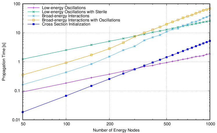
Figure 2: Propagation time scaling with problem size on Machine 1. Only the time to run EvolveState is included, omitting cross-section preparation time for the cases with interactions. This initialization can be separated by calling InitializeInteractions manually, and is shown as ‘Cross Section Initialization’. Propagation with only oscillation effects shows scaling which is very close to linear in the number of energies, while propagation with interactions takes time which is approximately quadratic in the number of energies.

Several tests were performed to demonstrate how the time to perform multi-energy propagations scales with the number of energy nodes included, depending on the use of some of the library’s major features. The results of these tests are shown in Fig. 2.

The ‘Low-energy Oscillations’ tests used a flat input spectrum over an energy range of 1 GeV - 10 GeV, initially consisting of $\nu_{\mu}$ only. For these tests, non-coherent interactions were disabled. The ‘Broad-energy Interactions’ test used an $E^{-2}$ input spectrum over 10 GeV - $10^{7}$ GeV with an initially equal mixture of flavors. All tests propagated the input flux through the full diameter of the Earth, using nuSQuIDS version of PREM for the density. Each propagation was tested for various sets of energy nodes, distributed uniformly in the logarithm of energy, from 50 to 1000 nodes, in increments of 50. Each measurement was repeated five times, and the median duration reported, unless the standard deviation of the distribution was greater than 1% of the mean, which was taken to indicate an unstable set of measurements, in which case the entire set of measurements was repeated.

The oscillation-only propagations are expected to scale linearly with the number of nodes, as the calculation performed for each integration step consists primarily of evolving the flavor projectors (needed to compute $H_{1}(E,x)$ and $H^{*}_{1}(E,x)$) and commutator forming the first terms on the right hand sides of Eqs. 10, which must be repeated for each energy node, neutrino flavor, and particle type (neutrino and anti-neutrino). This is borne out quite well by the measurements.

The oscillation calculation including a fourth, sterile neutrino flavor (‘Low-energy Oscillations with Sterile’) is significantly slower than the standard three-flavor calculation (‘Low-energy Oscillations’), as is to be expected. The representation of the four-flavor state for each component has sixteen components to the three-flavor state’s nine, so a decrease in speed of at least $16/9=1.77$ times may be expected, to start with. The addition of the sterile flavor also forces the ODE integrator to use a smaller step size for the integration, taking nearly eight times as many steps to complete the propagation. The combination of these effects seems to plausibly account for the observed decrease in speed.

The time for propagations, including non-coherent interactions (‘Broad-energy Interactions’), can be expected to scale quadratically in the number of energy nodes, due to the need to calculate the cascading of particles at each node down to all lower energy nodes. In addition, calculating the interactions requires an additional initialization step, in which the cross section data governing the cascading processes is gathered. Since this extra step is needed only once for a nuSQUIDS object to be able to perform multiple propagations with the same set of energy nodes, which is often relevant as various hypothesis input fluxes are tested, it is accounted separately in Fig. 2 as ‘Cross Section Initialization’. Both the cross section initialization and the propagations with interactions show approximately the expected quadratic scaling, and the calculation of both interactions and oscillations together (‘Broad-energy Interactions with Oscillations’) exhibits the additional cost of including both types of effects. A brief departure from the expected power law form of the propagation time scaling is observed at intermediate numbers of energy nodes is also observed for the tests with interactions; in Fig. 2, this appears approximately between 200 and 300 energy nodes. This is believed to be a result of the calculation’s memory use growing comparable in size to the CPU’s last-level cache (8 MB, for Machine 1). It appears reliably, but moves to higher node counts for CPUs with larger cache sizes. See Sec. 6.4 for a discussion of memory use and some representative numbers which support this hypothesis.

6.3 Flux Evaluation Performance

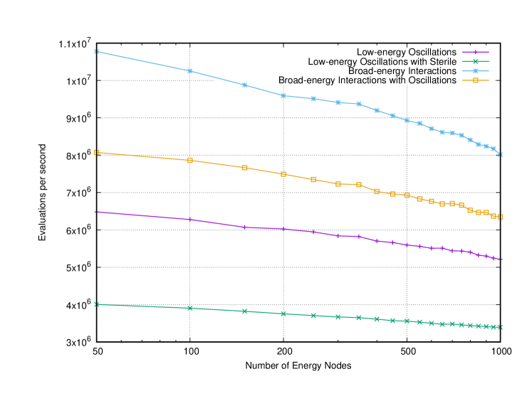
Figure 3: Flux evaluation speed scaling with problem size on Machine 1. As expected, only a weak dependence on the problem size is observed.

The purpose of propagating a flux with nuSQuIDS is to determine the spectrum or composition after propagation, so the efficiency with which this information can be extracted is the second critical half of the library’s performance.

Evaluation of the propagated flux for a given energy, flavor, particle type combination consists of three parts: Mapping the physical energy to a logical position within the energy nodes of the propagated state, interpolating the state components from the nearest nodes to form the requested state, and application of the suitably evolved $H_{0}$ operator to that state. Locating the nearest energy nodes for interpolation depends on the total number of such nodes, due to the allowance for arbitrary node distributions, and is performed using a binary search. The interpolation of the state, computation and evolution of the $H_{0}$ operator, and application of the operator to the interpolated state do not depend on the number of nodes, but do depend on the size of each state component, determined by the number of neutrino flavors considered.

Fig. 3 shows how the rate of flux evaluations scales with the number of energy nodes treated for the four example problems introduced in Sec. 6.2. As expected, due to the binary search for adjacent nodes, a weak dependence on number of nodes is observed. A marked drop in performance also occurs between the three-flavor and four-flavor oscillation calculations, as expected from the corresponding increase in the complexity of both the states and operators.

6.3.1 Concurrent Evaluation

Figure 4: Flux evaluation speed scaling with number of threads. Fairly good linearity is observed on both machines until the number of physical CPU cores is exhausted, at 4 and 16 threads, respectively. Both processors tested support 2-way simultaneous multithreading, but using it for this task is not productive on Machine 1 as shown by the lack of significant increase in total throughput when the number of threads is increased from 4 to 8, while Machine 2 initially suffers a penalty (the drop in throughput from 16 to 17 threads), but recovers and shows increased throughput as all logical CPU cores are used.

The nuSQUIDS object is not generally concurrency-safe for modification, but concurrent use of non-modifying member functions, including EvalFlavor, is safe and supported. This is potentially useful when computing large numbers of flux evaluations for tasks such as weighting large numbers of simulated neutrino interactions in a detector to form an expected observation. Fig. 4 shows an example of the application of this technique to evaluating the flux computed by the ‘Low Energy Oscillations’ calculation introduced previously. A problem size of 200 energy nodes was tested with a variable number of worker threads each being assigned to perform $10^{7}$ flux evaluations. Due to the limited number of processor cores available to Machine 1, a second hardware configuration was introduced for this test. Machine 2 used an AMD Ryzen™ 9 3950X CPU, having a ‘base’ operating frequency of 3.5 GHz, with frequency scaling disabled.

Scaling to many flux evaluation threads appears to work well until the number of physical CPU cores is saturated, in spite of memory allocations which are required by the internals of the calculation. An important optimization to enable this result was thread-local reuse of memory buffers, avoiding the need to serialize execution between threads even when the system memory allocator might use globally shared state. For numbers of evaluation threads beyond the available number of physical processor cores, simultaneous multithreading (SMT) is used, and produces mixed results which depend significantly on the CPU architecture. SMT does not enable a useful increase in throughput for Machine 1, while on Machine 2, additional SMT threads provide less marginal benefit than full physical cores, but aside from a small loss in total throughput when a small number of physical cores are running multiple SMT threads, throughput generally benefits. As this is not a thorough survey of available CPU models, users are advised to perform their own checks to determine whether use of SMT will be productive on their hardware.

6.4 Memory Requirements

For a nuSQuIDS object configured with $M$ energy nodes, $N$ neutrino flavors, $P$ particle types, and $T$ target species for interactions (if non-coherent interactions are enabled), neglecting constant terms, the amount of memory used may be broken down as follows. Essentially all data allocated by the nuSQuIDS object is either in the form of machine pointers or double-precision floating-point numbers, assuming that the non-pointer components of squids::SU_vector are small enough that padding and alignment requirements fit them into space equivalent to two additional pointers, making the direct size of an SU_vector three pointers. The underlying squids::SQuIDS object then requires:

$$(PN^{2}+1)M$$ doubles (16a)

$$9(P+1)M$$ pointers (16b)

This omits some amount of memory which the GSL ODE integration library will allocate for its own internal state. The size of this state will be proportional to $PN^{2}M$ doubles, with the constant of proportionality typically being around 10 (e.g. it is 12 when using the nuSQuIDS default Runge-Kutta-Fehlberg 4-5 stepper, RKF45).

Without structures needed for non-coherent interactions, the nuSQuIDS object additionally allocates:

$$(2PN^{3}+N^{2}+6PN+5)M+(P+1)N^{3}+3(P+1)N$$ doubles (17a)

$$3(2PN+1)M+3(P+1)N$$ pointers (17b)

The data structures for computing non-coherent interactions (neglecting any memory allocated by the cross section and $\tau$ decay objects themselves) require:

$$(2(NT+1)P+1)M^{2}+(PN^{2}+(2T+3)PN+12)M$$ doubles (18a)

$$3PM$$ pointers (18b)

If the external neutrino source feature is used, it requires a buffer of another $PNM$ doubles.

It should be noted that $P$ can only take on the values 1 and 2, $T$ is typically 2, and $N$ is generally 3 or 4.

As an example, a modestly-sized three-flavor neutrino oscillation calculation might use 100 energy nodes and not consider non-coherent interactions, so $M=100$, $N=3$, $P=2$ (if both neutrinos and anti-neutrinos are considered), and $T$ is irrelevant. Assuming typical data sizes of 8 bytes for both pointers and double-precision floating-point numbers, such a calculation will then require $24435*8$ bytes or approximately 191 kilobytes of memory, plus approximately another 170 kilobytes allocated by GSL (for the RKF45 stepper).

Due to the quadratic scaling with number of energy nodes (of the differential charged- and neutral-current interaction cross sections and $\tau$ decay spectra), memory requirements are much higher for calculations with non-coherent interactions. An interaction calculation with 100 energy nodes and all interaction effects enabled would have $M=100$, $N=3$, $P=2$, and $T=2$, leading to a memory requirement of $322235*8$ bytes, or approximately 2.5 megabytes, and increasing to 300 nodes ($M=300$) would require $2706435*8$ bytes, or approximately 20.6 megabytes (with the size of the GSL state also increasing to 506 kilobytes). Use of the external neutrino source feature, even with this larger problem size, would require only an additional $1800*8$ bytes or 14 kilobytes.

6.5 Efficient Use

Besides configuring the number of energy nodes and the error tolerance to the lowest and loosest values which will provide the desired precision, there are several other considerations for using nuSQuIDS with the best possible efficiency.

One simple trick is to turn off features which are not needed for a given calculation. If neutrino oscillations are not relevant in the regime covered by a given propagation problem, they can be disabled, and the same is true for non-coherent interactions. With oscillations disabled, nuSQuIDS is able to skip computing the evolution of the flavor projection operators, and with interactions disabled it can omit obtaining interaction cross sections, updating interaction lengths for the matter density at each step, and computing the contribution to each energy node from the neutrinos cascading down from higher energy nodes. Additionally, some particular types of interactions can be enabled or disabled as needed, in particular, tau regeneration and Glashow resonance effects. For example, to propagate a high-energy atmospheric neutrino flux, not only are oscillations potentially unnecessary, but the flavor composition of the flux may mean the tau regeneration is irrelevant as well. If a flux is being calculated which involves no anti-neutrinos, the effects of the Glashow resonance will not appear, and they may be turned off without changing the result. In general, nuSQuIDS attempts to detect possibilities at runtime to minimize work performed, and this is fairly successful in the case of tau regeneration, so turning this feature off may not produce much change in computation time. Handling of the Glashow resonance, though, requires additional interaction length updates which the existing structure of the code is unable to optimize away even when it turns out to be unused, so turning this capability off when it is not needed can have a useful impact.

The cross-section data required to compute non-coherent interactions is dependent only on the placement of the energy nodes, not on the flux being propagated. As a result, if many fluxes are to be calculated over the same set of nodes, it is most efficient to reuse the same nuSQUIDS object, merely resetting the initial flux with Set_initial_state before calling EvolveState again, so that this initialization is not repeated. As shown in 2 the initialization can take 5-15% of the time for the propagation, so this can represent an important savings over many propagations.

7 Conclusions

nuSQUIDS  provides a complete solution to neutrino propagation while accounting for neutrino oscillations and scattering. We find that it is competitive with dedicated neutrino oscillation calculators, when the number of evaluations of the oscillation probability is large, which is the typical case of interest in neutrino experiments. The library also has a Python extension. Finally, the nuSQUIDS  library has been designed to be easily extendable to both new media and new physics scenarios. User contributions to the project are encouraged and a number of additional models have already been implemented and are linked in resources/user_contributions.

Appendix A Examples

To illustrate use of the library in concrete scenarios we provide a set of examples. These examples are located in different sub-folders inside a folder called examples. A specific example can be compiled using the makefile by running make examples example_name, and omitting the name compiles all the examples. Some of the examples contain a Gnuplot script to plot the output file.

A.1 Single energy (examples/Single_energy)

This example illustrates the use of the simplified mode to compute the propagation of the neutrinos for a single energy.

In the following we will go though the main file of the example. First, we construct the nuSQuIDS object using the signature that requires only the number of flavors and specification of the use of neutrinos or antineutrinos.

⬇

1 nuSQUIDS nus(3,neutrino);

We next set the value of the oscillation parameters, giving the values for the mixing angles in radians, the value for the mass square difference in electron-volt squared, and a value for the $CP$ phase in radians. In order to do so we use the Set_MixingAngle member function whose first two arguments are the indices of the rotation, starting from zero. The $CP$ phase function is similar. In the case of the square mass difference, the first argument of the function is the mass eigenvalue index and the second argument the value. These square mass differences are always with respect to the lightest mass state (whose index is zero).

⬇

27 nus.Set_MixingAngle(0,1,0.563942);

28 nus.Set_MixingAngle(0,2,0.154085);

29 nus.Set_MixingAngle(1,2,0.785398);

30

31 nus.Set_SquareMassDifference(1,7.65e-05);

32 nus.Set_SquareMassDifference(2,0.00247);

33

34 nus.Set_CPPhase(0,2,0.0);

We declare a structure that contains all the physical units and constants we will need.

⬇

1 squids::Const units;

This line sets the energy of the neutrino to be propagated.

⬇

34 nus.Set_E(10.0*units.GeV);

Next, we define the medium in which we are going to propagate the neutrinos. The atmospheric Earth object used here, earth_atm, contains the geometry and density of the Earth, including a simple treatment of the atmosphere; see A.4 for more details. We also construct a trajectory in the earth for a zenith angle phi, earth_atm_track. Finally, we apply these objects to the nuSQuIDS object.

⬇

1 double phi = acos(-1.0);

2 auto earth_atm = std::make_shared<EarthAtm>();

3 auto earth_atm_track = std::make_shared<EarthAtm::Track>(

4 earth_atm->MakeTrackWithCosine(phi));

5 nus.Set_Body(earth_atm);

6 nus.Set_Track(earth_atm_track);

Now we set the initial neutrino flavor composition. In this example we start with a pure muon neutrino state, represented by an marray (multi-dimensional array) of rank 1 and length {3}, corresponding to the number of flavors, and with value given by {0,1,0}. We indicate that this state is described in the flavor basis when applying it to the nuSQuIDS object:

⬇

34 marray<double,1> ini_state({3},{0,1,0});

35 nus.Set_initial_state(ini_state,flavor);

We set the numerical error for the GSL differential equation solver. The parameters and errors are defined as in the standard GSL libraries.

⬇

6 nus.Set_rel_error(1.0e-20);

7 nus.Set_abs_error(1.0e-20);

Finally, we show the result before and after propagation. The propagation is done by calling the function nus.EvolveState()

⬇

35 std::cout << "In␣state" << std::endl;

36 for (double EE : nus.GetERange()){

37 std::cout << EE/units.GeV << "␣";

38 for(int i = 0; i < 3; i++){

39 std::cout << nus.EvalFlavor(i) << "␣";

40 }

41 std::cout << std::endl;

42 }

43 // We do the calculation

44 nus.EvolveState();

45

46 // Output the result

47 std::cout << "Out␣state" << std::endl;

48 for (double EE : nus.GetERange()){

49 std::cout << EE/units.GeV << "␣";

50 for(int i = 0; i < 3; i++){

51 std::cout << nus.EvalFlavor(i) << "␣";

52 }

53 std::cout << std::endl;

54 }

A.2 Multiple Energy (examples/Multiple_energy)

This is a more realistic example where we consider an ensemble of neutrinos in an energy range. With this setup, we can model the neutrino energy and flavor changes, including the effects of charged and neutral current interactions. In the following we describe the code for the example.

As before, we construct the Const object to have a set of useful physical parameters.

⬇

1 squids::Const units;

In the following, we allow the choice to compute the propagation for three active neutrinos or three active and one sterile.

⬇

54 std::cout << "(3)␣Three␣Active␣Neutrinos,␣" << "(4)␣3+1␣Three␣Active␣and␣One␣Sterile␣Neutrino" << std::endl;

55 unsigned int numneu;

56 std::cin >>numneu;

57 if( not(numneu==3 || numneu==4)){

58 throw std::runtime_error("Only␣(3)␣or␣(4)␣are␣valid␣options");

59 }

In the next line, we construct the nuSQUIDS object. For the multiple energy constructor, we need to provide the following arguments: a list of neutrino energy nodes (logspace(1.*units.GeV,1.e4*units.GeV,200)), number of neutrino flavors (numneu= 3 or 4), neutrino or anti-neutrino type (neutrino), and whether to compute non-coherent scattering interactions (false).

⬇

8 nuSQUIDS nus(logspace(1.*units.GeV,1.e4*units.GeV,200),numneu,neutrino,false);

As in the single energy mode, we must define the body and the path where neutrinos will propagate.

⬇

59 double phi = acos(-1.);

60 auto earth_atm = std::make_shared<EarthAtm>();

61 auto track_atm = std::make_shared<EarthAtm::Track>(

62 earth_atm->MakeTrackWithCosine(phi));

63 nus.Set_Body(earth_atm);

64 nus.Set_Track(track_atm);

We set the neutrino oscillation parameters, and if a sterile neutrino is considered, we set its parameters to $\theta_{24}=0.1$ and $\Delta m_{41}^{2}=0.1{\rm eV}^{2}$.

⬇

8 nus.Set_MixingAngle(0,1,0.563942);

9 nus.Set_MixingAngle(0,2,0.154085);

10 nus.Set_MixingAngle(1,2,0.785398);

11 nus.Set_SquareMassDifference(1,7.65e-05);

12 nus.Set_SquareMassDifference(2,0.00247);

13

14 if(numneu==4){ // sterile neutrino parameters

15 nus.Set_SquareMassDifference(3,0.1);

16 nus.Set_MixingAngle(1,3,0.1);

17 }

Next we set some of the integration parameters: the maximum step size for the evolution, the GSL stepper algorithm (all the steppers in the GSL libraries can be used), and maximum relative and absolute error tolerances.

⬇

64 nus.Set_h_max( 500.0*units.km );

65 nus.Set_GSL_step(gsl_odeiv2_step_rk4);

66 nus.Set_rel_error(1.0e-5);

67 nus.Set_abs_error(1.0e-5);

We set to true the progress bar options in order to display the progress of the propagation.

⬇

17 nus.Set_ProgressBar(true);

We can ask nuSQuIDS to give back the array containing the values of the energy nodes. We use this here to fill a multi-dimensional array with the initial state of the system; in this case a $E^{-2}$ power-law for the muon flavor and zero for the other flavors. Unlike the single-energy example, the array now has rank 2, with dimensions for both energy and flavor.

⬇

67 marray<double,1> E_range = nus.GetERange();

68 marray<double,2> inistate{E_range.size(),numneu};

69 double N0 = 1.0e18;

70 for ( int i = 0 ; i < inistate.extent(0); i++){

71 for ( int k = 0; k < inistate.extent(1); k ++){

72 inistate[i][k] = (k == 1) ? N0*pow(E_range[i],-2) : 0.0;

73 }

74 }

75 nus.Set_initial_state(inistate,flavor);

We can then evolve the state:

⬇

17 nus.EvolveState();

Finally, we write the propagated fluxes to a file and ask whether to run the plotting script:

⬇

75 std::ofstream file("fluxes_flavor.txt");

76

77 int Nen =1000;

78 double lEmin=0;

79 double lEmax=4;

80

81 file << "#␣log10(E)␣E␣flux_i␣fluxRatio_i␣.␣.␣.␣." << std::endl;

82 for(double lE=lEmin; lE<lEmax; lE+=(lEmax-lEmin)/(double)Nen){

83 double E=pow(10.0,lE)*units.GeV;

84 file << lE << "␣" << E << "␣";

85 for(int fl=0; fl<numneu; fl++){

86 file << "␣" << nus.EvalFlavor(fl, E) << "␣" << nus.EvalFlavor(fl, E)/(N0*pow(E,-2));

87 }

88 file << std::endl;

89 }

90 file.close();

91 std::string plt;

92 std::cout << std::endl << "Done!␣" << std::endl <<

93 "␣␣Do␣you␣want␣to␣run␣the␣gnuplot␣script?␣yes/no" << std::endl;

94 std::cin >> plt;

95 if(plt=="yes" || plt=="y")

96 return system("./plot.plt");

Note that while we explicitly propagated 200 energies, we evaluate the resulting flux at 1000 energies, taking advantage of the automatic interpolation.

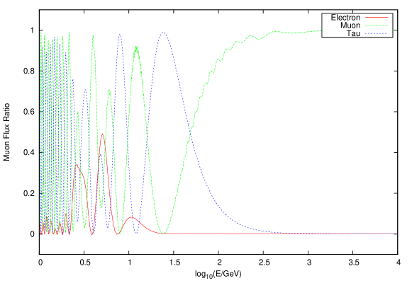
Figure 5: Output for the multiple-energy mode with sterile neutrino (3+1)

In Fig. 5, we show the results of running this example for the case with sterile neutrino.

A.3 Read and Write (examples/HDF5_Write_Read)

In this example, we illustrate the use of the functions to read and write HDF5 files. The file contains the full information of the system: all settings, body, track (including the current position along the track), and the density matrix at each node. This serialization allows saving the system in the middle of a complex propagation, and reading it later to continue the calculation. Saving the system and then loading it from the file restores the system to the saved state, allowing the user to compute any quantum-mechanical observable.

This example is based upon the multiple energy example, but split into two parts. The first part computes the evolution and saves the state of the system (write.cpp). The second reads the state, extracts the flavor fluxes, and prints them to a file (read.cpp).

In the following, we describe lines that are relevant for reading and writing.

In the file write.cpp, we save the system before and after the evolution:

⬇

1 nus.WriteStateHDF5("./initial_state.hdf5");

2 nus.EvolveState();

3 nus.WriteStateHDF5("./final_state.hdf5");

In order to recover that state in read.cpp, we use the constructor that takes the name of the file as an argument:

⬇

1 nuSQUIDS inus("./initial_state.hdf5");

2 nuSQUIDS fnus("./final_state.hdf5");

A.4 Construction and use of bodies (examples/Bodies)

Two of the main classes in the nuSQuIDS library are the body and the track. These properties of the nuSQuIDS object itself do not have defaults, and always need to be specified. In this example, we show how to use the objects already implemented in the library, and also how to create derived types from the classes already defined.

The folder examples/Bodies/ contains new body and track definitions in the files exBody.h and exBody.cpp. It also contains the file main.cpp, whose main function uses all the pre-existing objects in nuSQUIDS and the new objects of these examples.

A.4.1 Construct a derived body

Here is an example of how to define a derived class from the EarthAtm body. In this simple case the object is just an Earth model with some parameters that weight the relative densities in the different layers of the Earth’s inner core, outer core, and mantle.

The new classes may be placed inside the nusquids namespace. We define a new class called EarthMod, which is a derived class of EarthAtm. Because of this, the new class will have all the properties, values, and functions of the parent class.

⬇

1namespace nusquids{

2

3class EarthMod: public EarthAtm{

4public:

Our object’s constructors require the following inputs: base Earth model file name (earthmodel), inner core weight (frho1), outer core weight (frho2), and mantle weight (frho3).

⬇

2 EarthMod(std::string earthmodel, double frho1, double frho2, double frho3);

The Mod function allows changing the parameters once the object is already initialized.

⬇

4 void Mod(double frho1, double frho2, double frho3);

5};

The implementations of the functions that set the density arrays with the modified values are given in the file exBody.cpp.

A.4.2 Use of the bodies

The main.cpp file defines a nuSQUIDS object and sets different bodies and tracks. For each of these, it evolves the system and displays the resulting oscillation probabilities. For simplicity we use the single energy mode Sec. A.1, but the use of the body and track would be the same for the multiple energy case.

First, we construct the nuSQUIDS object for three neutrinos, then we set the oscillation parameters and the neutrino energy.

⬇

1 nuSQUIDS nus(3,neutrino);

2 nus.Set_MixingAngle(0,1,0.563942);

3 nus.Set_MixingAngle(0,2,0.154085);

4 nus.Set_MixingAngle(1,2,0.785398);

5 nus.Set_SquareMassDifference(1,7.65e-05);

6 nus.Set_SquareMassDifference(2,0.00247);

7 nus.Set_CPPhase(0,2,0.0);

8 squids::Const units;

9 nus.Set_E(10.0*units.GeV);

1. Earth

   The first example is the Earth body. In this case, the track is parametrized by the chord length through the Earth, which is useful for treating the baseline of an experiment with a fixed source and detector. Here we define the body and track. For the track we need to specify the initial and final position as well as the baseline:

   ⬇

   5 double baseline = 500.0*units.km;

   6 std::shared_ptr<Earth> earth = std::make_shared<Earth>();

   7 std::shared_ptr<Earth::Track> earth_track = std::make_shared<Earth::Track>(0.0,baseline,baseline);

   We apply the Body and Track to the nuSQuIDS object:

   ⬇

   9 nus.Set_Body(earth);

   10 nus.Set_Track(earth_track);

   We then set the initial state of the system and print it:

   ⬇

   7 marray<double,1> ini_state({3},{0,1,0});

   8 nus.Set_initial_state(ini_state,flavor);

   9

   10 std::cout << "In␣state" << std::endl;

   11 for (double EE : nus.GetERange()){

   12 std::cout << EE/units.GeV << "␣";

   13 for(int i = 0; i < 3; i++){

   14 std::cout << nus.EvalFlavor(i) << "␣";

   15 }

   16 std::cout << std::endl;

   17 }

   We set the numerical error and maximum step for the GSL integrator:

   ⬇

   10 nus.Set_h_max( 200.0*units.km );

   11 nus.Set_rel_error(1.0e-12);

   12 nus.Set_abs_error(1.0e-12);

   Finally, we evolve the state and print it:

   ⬇

   17 nus.EvolveState();

   18 std::cout << "Out␣state" << std::endl;

   19 for (double EE : nus.GetERange()){

   20 std::cout << EE/units.GeV << "␣";

   21 for(int i = 0; i < 3; i++){

   22 std::cout << nus.EvalFlavor(i) << "␣";

   23 }

   24 std::cout << std::endl;

   25 }

   These last steps in the code are the same in all the bodies examples and so are omitted for the following cases.

2. EarthAtm

   In this example we use the EarthAtm body. This body includes both the Earth and its atmosphere. The track is defined by the zenith angle of the trajectory, and begins at the top of the atmosphere. Because the track depends on the height of the atmosphere being treated, it is most conveniently constructed from the body, using the MakeTrack function, which takes a zenith angle and creates a track with the necessary details of the body automatically included.

   ⬇

   12 double phi = acos(-1.0);

   13 auto earth_atm = std::make_shared<EarthAtm>();

   14 auto earth_atm_track = std::make_shared<EarthAtm::Track>(earth_atm->MakeTrack(phi));

   15

   16 nus.Set_Body(earth_atm);

   17 nus.Set_Track(earth_atm_track);

3. earth_mod

   In this case, we use the modified Earth object. As for the EarthAtm object, the track is defined by the zenith angle of the trajectory. In the constructor we set all the weights to $0.1$. Finally, we set the body and track for the nuSQUIDS object.

   ⬇

   25 double phi = acos(-1.0);

   26 std::shared_ptr<EarthMod> earth_mod = std::make_shared<EarthMod>(0.1,0.1,0.1);

   27 std::shared_ptr<EarthMod::Track> earth_mod_track = std::make_shared<EarthMod::Track>(phi);

   28

   29 nus.Set_Body(earth_mod);

   30 nus.Set_Track(earth_mod_track);

4. VariableDensity

   In this case, we use the variable density body and a track of $200{\rm km}$. First, we define the density, position, and electron fraction arrays with the corresponding values.

   ⬇

   17 int N=40;

   18

   19 std::vector<double> x_arr(N);

   20 std::vector<double> density_arr(N);

   21 std::vector<double> ye_arr(N);

   22

   23 double size = 1000.0*units.km;

   24 for(int i = 0; i < N; i++){

   25 x_arr[i] = size*(i/(double)N);

   26 density_arr[i] = fabs(cos((double)i));

   27 ye_arr[i] = fabs(sin((double)i));

   28 }

   Now we construct the body and the track. The constructor for the variable density takes as an input the position, density, and electron fraction vectors. Finally, like before, we set the body and the track on the nuSQUIDS object.

   ⬇

   30

   31 std::shared_ptr<VariableDensity> vardens = std::make_shared<VariableDensity>(x_arr,density_arr,ye_arr);

   32 std::shared_ptr<VariableDensity::Track> track_vardens = std::make_shared<VariableDensity::Track>(0.0,200.0*units.km);

   33

   34 nus.Set_Body(vardens);

   35 nus.Set_Track(track_vardens);

5. Vacuum

   This is a trivial case where the density and electron fraction are zero. We only need to give the baseline as an argument to construct the track. In this example, we set the baseline to $500{\rm km}$.

   ⬇

   28 double baseline_2 = 500.0*units.km;

   29 std::shared_ptr<Vacuum> vacuum = std::make_shared<Vacuum>();

   30 std::shared_ptr<Vacuum::Track> track_vac = std::make_shared<Vacuum::Track>(baseline_2);

   31

   32 nus.Set_Body(vacuum);

   33 nus.Set_Track(track_vac);

6. ConstantDensity

   In the case of constant density an analytic approximation can be used to propagate the neutrinos if non-coherent interactions are disabled in the construction of the nuSQUIDS object. The full Hamiltonian of the system is diagonalized and exponentiated.

   We set the density to $100{\rm g/cm}^{3}$, the electron fraction to $0.3$, and the baseline to $500{\rm km}$.

   ⬇

   35

   36 double density = 100.0;

   37 double ye = 0.3;

   38 std::shared_ptr<ConstantDensity> constdens = std::make_shared<ConstantDensity>(density,ye);

   39 double baseline_3 = 500.0*units.km;

   40 std::shared_ptr<ConstantDensity::Track> track_constdens = std::make_shared<ConstantDensity::Track>(0.0,baseline_3);

   41

   42 nus.Set_Body(constdens);

   43 nus.Set_Track(track_constdens);

A.5 Cross Sections (examples/Xsections)

One of the important features of nuSQuIDS is the possibility of consistently handling non-coherent interactions and oscillation behavior. The physical quantity that encodes how often these scattering interactions happen between the neutrinos and the media is the cross section. nuSQuIDS has implemented two kinds of deep inelastic scattering (DIS) interactions: charged- and neutral-current, as well as resonant $W^{-}$ production on electrons (the Glashow resonance). It takes into account the neutrinos produced by the decay of short lived charged particles such as $\tau^{\pm}$ and $W^{\pm}$. For the neutral-current, we always include the outgoing neutrino. Other particles produced in the interactions, such as hadrons or long-lived charged leptons, are ignored along the evolution. This information is organized and stored in the cross-section class. This class requires the user to provide the total cross-section for each flavor and current in units of cm². It also requires the singly-differential neutrino cross-sections with respect to the outgoing neutrino energy in units of cm²/GeV. See  B.2.3 for more details of how this data must be specified.

nuSQuIDS includes by default deep inelastic neutrino-nucleon cross-sections as well as neutrino-electron cross-sections [102, 128].

In this example, we construct a new cross section object to be used by nuSQuIDS instead of the default one. Every cross section must be a class of NeutrinoCrossSections and implement at least two member functions: SingleDifferentialCrossSection and TotalCrossSection.

⬇

1 class LinearCrossSections : public NeutrinoCrossSections {

2 private:

3 const squids::Const units;

4 const double GF = 1.16639e-23; // eV^-2

5 const double mp = 938.272e6; // proton mass eV

6 const double CC_to_NC; // proportion of CC to NC which goes from 0 to 1.

7 public :

8 LinearCrossSections(double CC_to_NC):CC_to_NC(CC_to_NC){assert( CC_to_NC <= 1.0 && CC_to_NC >= 0.0 );}

9 LinearCrossSections():LinearCrossSections(0.5){}

10 double TotalCrossSection(double Enu, NeutrinoFlavor flavor, NeutrinoType neutype, Current current) const override;

11 double SingleDifferentialCrossSection(double E1, double E2, NeutrinoFlavor flavor, NeutrinoType neutype, Current current) const override;

12 };

We use a toy total cross section that scales linearly with the neutrino energy and the corresponding differential cross sections linear in the outgoing neutrino energy; see implementation in exCross.cpp. We also allow changing the proportion of charge-to-neutral current at the construction of the object.

We construct two cross section libraries with the new cross section associated with an isoscalar nucleon target: one with only charged-current interactions ncs_cc and another with only neutral-current ncs_nc. Then we construct the corresponding nuSQUIDS objects nus_cc and nus_nc. We also disable neutrino oscillations in this example by means of the option Set_IncludeOscillations(false).

⬇

1 auto ncs_cc=std::make_shared<CrossSectionLibrary>(CrossSectionLibrary::MapType{

2 {isoscalar_nucleon, std::make_shared<LinearCrossSections>(0.0)}});

3 auto ncs_nc=std::make_shared<CrossSectionLibrary>(CrossSectionLibrary::MapType{

4 {isoscalar_nucleon, std::make_shared<LinearCrossSections>(1.0)}});

5

6 nuSQUIDS nus_cc(logspace(Emin,Emax,200),numneu,neutrino,true,ncs_cc);

7 nus_cc.Set_IncludeOscillations(false);

8 nuSQUIDS nus_nc(logspace(Emin,Emax,200),numneu,neutrino,true,ncs_nc);

9 nus_nc.Set_IncludeOscillations(false);

We can see the final to initial flux ratios for both cases in fig 6.

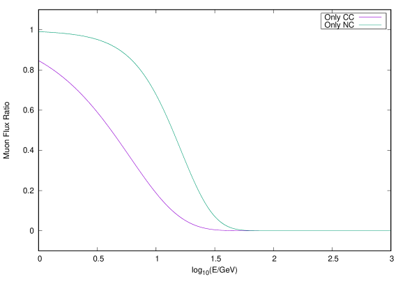
Figure 6: Final to initial flux ratio as a function of the logarithm of the neutrino energy for the example toy cross-sections with only charged-current (CC) and only neutral-current (NC) interactions.

A.6 Constant density multiple layers (examples/Constant_density_layers)

Since the constant density allows us to do very fast computation using the diagonalization of the full Hamiltonian here we show an example where we concatenate the evolution of the neutrinos through different layers of constant density.

We construct three different layers: first $100{\rm km}$ in vacuum, second $50{\rm km}$ in matter with density $3.5{\rm g/cm}^{3}$ and electron fraction $0.5$, and finally $200{\rm km}$ in matter with density $10{\rm g/cm}^{3}$ and electron fraction $0.1$.

⬇

1 const double layer_1 = 100.*units.km;

2 std::shared_ptr<Vacuum> vacuum = std::make_shared<Vacuum>();

3 std::shared_ptr<Vacuum::Track> track_env0 = std::make_shared<Vacuum::Track>(layer_1);

4

5 const double layer_2 = 50.*units.km;

6 std::shared_ptr<ConstantDensity> constdens_env1 = std::make_shared<ConstantDensity>(3.5,0.5);

7 std::shared_ptr<ConstantDensity::Track> track_env1 = std::make_shared<ConstantDensity::Track>(layer_2);

8

9 const double layer_3 = 200.*units.km;

10 std::shared_ptr<ConstantDensity> constdens_env2 = std::make_shared<ConstantDensity>(10.,0.1);

11 std::shared_ptr<ConstantDensity::Track> track_env2 = std::make_shared<ConstantDensity::Track>(layer_3);

Now in order to evolve the system we set the corresponding body and track and evolve every layer.

⬇

1 nus.Set_Body(vacuum);

2 nus.Set_Track(track_env0);

3 nus.EvolveState();

4

5 nus.Set_Body(constdens_env1);

6 nus.Set_Track(track_env1);

7 nus.EvolveState();

8

9 nus.Set_Body(constdens_env2);

10 nus.Set_Track(track_env2);

11 nus.EvolveState();

Finally, we write the output for the different flavor fluxes in a text file.

A.7 BSM extension: Non-Standard Interaction (NSI) (examples/NSI)

In this example we illustrate how to construct a derived class of nuSQUIDS including a new physics term. This procedure is similar to other new physics setups A.8.

The implementation of nuSQUIDSNSI class is in NSI.h. We will go through the implementation to see what needs to be added to the base class.

First, we declare the NSI matter potential as a SU_vector called NSI. By default nuSQuIDS works in the interaction picture, thus every term we add to the Hamiltonian has to be properly evolved with $H_{0}$. Since $H_{0}$ depends on the energy we do this in every node. For optimization we will compute and store the evolved NSI term in a vector of SU_vector objects called NSI_evol.

The HI_prefactor contains all the numerical factors multiplying the operator and epsilon_mutau is the strength of the NSI $\mu$-$\tau$ non-diagonal component. Notice that we set all other NSI contributions to zero.

⬇

1class nuSQUIDSNSI: public nuSQUIDS {

2 private:

3 squids::SU_vector NSI;

4 std::vector<squids::SU_vector> NSI_evol;

5 std::unique_ptr<double[]> hiBuffer;

6 double HI_prefactor;

7 // nsi parameters

8 double epsilon_mutau;

As previously noted, we need to compute the NSI operator in the interaction picture prior to adding it to the r.h.s. of the differential equation. We compute this for every energy node in the AddToPreDerive function. This function is called inside the PreDerive function before evaluating the derivatives to allow the user to pre-compute terms used in the derivative. The evolution of the NSI term by $H_{0}$ is done by the SU_vector::Evolve member. This function is optimized and performs the evolution of the operator analytically.

⬇

11 void AddToPreDerive(double x){

12 for(int ei = 0; ei < ne; ei++){

13 NSI_evol[ei] = NSI.Evolve(H0_array[ei],(x-Get_t_initial()));

14 }

15 }

The following auxiliary member functions allow nuSQUIDSNSI to save the new physics parameters into the hdf5 files when the WriteStateHDF5 is called (See Sec. A.3 for an overview of reading and writing).

⬇

8 void AddToReadHDF5(hid_t hdf5_loc_id){

9 // here we read the new parameters now saved in the HDF5 file

10 hid_t nsi = H5Gopen(hdf5_loc_id, "nsi", H5P_DEFAULT);

11 H5LTget_attribute_double(hdf5_loc_id,"nsi","mu_tau" ,&epsilon_mutau);

12 H5Gclose(nsi);

13 }

14

15 void AddToWriteHDF5(hid_t hdf5_loc_id) const {

16 // here we write the new parameters to be saved in the HDF5 file

17 H5Gcreate(hdf5_loc_id, "nsi", H5P_DEFAULT, H5P_DEFAULT, H5P_DEFAULT);

18 H5LTset_attribute_double(hdf5_loc_id, "nsi","mu_tau",&epsilon_mutau, 1);

19 }

Here we overload the HI function where we return the original nuSQUIDS matter potential plus the new NSI contribution.

⬇

15 squids::SU_vector HI(unsigned int ei,unsigned int index_rho) const{

16 double CC=HI_prefactor*body->density(*track)*body->ye(*track);

17

18 squids::SU_vector potential(nsun,hiBuffer.get());

19

20 potential = (3.0*CC)*NSI_evol[ei];

21

22 if ((index_rho == 0 and NT==both) or NT==neutrino){

23 return nuSQUIDS::HI(ei,index_rho) + potential;

24 } else if ((index_rho == 1 and NT==both) or NT==antineutrino){

25 return nuSQUIDS::HI(ei,index_rho) + (-1.0)*std::move(potential);

26 } else{

27 throw std::runtime_error("nuSQUIDS::HI␣:␣unknown␣particle␣or␣antiparticle");

28 }

29 }

The constructor first calls the nuSQUIDS constructor and then sets the oscillation parameters and the NSI operator.

⬇

19 public:

20 nuSQUIDSNSI(double epsilon_mutau, marray<double,1> Erange,

21 int numneu, NeutrinoType NT, bool iinteraction,

22 double th01=0.563, double th02=0.154, double th12=0.785):

23 nuSQUIDS(Erange,numneu,NT,iinteraction),

24 hiBuffer(new double[nsun*nsun]),

25 epsilon_mutau(epsilon_mutau)

26 {

27 assert(numneu == 3);

28 // defining a complex matrix M which will contain our flavor

29 // violating flavor structure.

30 gsl_matrix_complex * M = gsl_matrix_complex_calloc(3,3);

31 gsl_complex c {{ epsilon_mutau , 0.0 }};

32 gsl_matrix_complex_set(M,2,1,c);

33 gsl_matrix_complex_set(M,1,2,gsl_complex_conjugate(c));

34

35 NSI = squids::SU_vector(M);

36

37 Set_MixingAngle(0,1,th01);

38 Set_MixingAngle(0,2,th02);

39 Set_MixingAngle(1,2,th12);

40

41 // rotate to mass reprentation

42 NSI.RotateToB1(params);

43 NSI_evol.resize(ne);

44 for(int ei = 0; ei < ne; ei++){

45 NSI_evol[ei] = squids::SU_vector(nsun);

46 }

47 gsl_matrix_complex_free(M);

48

49 HI_prefactor = params.sqrt2*params.GF*params.Na*pow(params.cm,-3);

50 }

The next function sets the value of epsilon_mutau changing the SU_vector NSI object accordingly. We construct the SU_vector operator as a complex GSL matrix that represents the operator in the flavor basis. Since nuSQuIDS solves the propagation in the basis where $H_{0}$ is diagonal, i.e. the mass basis, we rotate the NSI operator to the mass basis by calling RotateToB1.

⬇

29 void Set_mutau(double eps){

30 gsl_matrix_complex * M = gsl_matrix_complex_calloc(3,3);

31 gsl_complex c {{ epsilon_mutau , 0.0 }};

32 gsl_matrix_complex_set(M,2,1,c);

33 gsl_matrix_complex_set(M,1,2,gsl_complex_conjugate(c));

34 NSI = squids::SU_vector(M);

35 NSI.RotateToB1(params);

36 gsl_matrix_complex_free(M);

37 }

In main.cpp we use the new NSI class in a multiple energy mode. In order to compare the oscillation probabilities with and without NSI we construct two instances of nuSQUIDSNSI with epsilon_mutau=0 and epsilon_mutau=1e-2.

⬇

50 double eps_mutau=1.0e-2;

51 nuSQUIDSNSI nus(eps_mutau,logspace(Emin,Emax,200),numneu,antineutrino,false);

52 nuSQUIDSNSI nus_zero(0.0,logspace(Emin,Emax,200),numneu,antineutrino,false);

In the next lines we propagate both objects and print both fluxes to a file.

⬇

37 nus.EvolveState();

38 nus_zero.EvolveState();

39

40 int Nen =1000;

41 double lEmin=log10(Emin);

42 double lEmax=log10(Emax);

43

44 std::ofstream file("fluxes_flavor.txt");

45

46 file << "#␣log10(E)␣E␣flux_NSI_i␣flux_noNSI_i␣.␣.␣.␣." << std::endl;

47 for(double lE=lEmin; lE<lEmax; lE+=(lEmax-lEmin)/(double)Nen){

48 double E=pow(10.0,lE);

49 file << lE << "␣" << E << "␣";

50 for(int fl=0; fl<numneu; fl++){

51 file << "␣" << nus.EvalFlavor(fl, E) << "␣" << nus_zero.EvalFlavor(fl, E);

52 }

53 file << std::endl;

54 }

In the folder there is a script that allows plotting the output text file.

A.8 BSM extension: Lorentz Violation (examples/LV)

The Lorentz symmetry is a well established property of space-time. As a fundamental symmetry, it should be tested and neutrino oscillations probe part of the parameter space.

The example is technically the same as the non-standard interactions, but we add a couple of features to illustrate good practices.

As before, the new term is added in to HI. For this particular physics case the effect is positive for neutrinos and negative for antineutrinos. This can be implemented using the integer irho which labels neutrinos with $0$ and antineutrinos with $1$ when both particle types are being calculated. Which particle types are under consideration is given by the NT member variable.

⬇

52 squids:: SU_vector HI(unsigned int ie,unsigned int irho) const {

53 squids::SU_vector potential = nuSQUIDS::HI(ie, irho);

54 double sign = 1;

55 if ((irho == 1 and NT==both) or NT==antineutrino){

56 // antineutrino matter potential flips sign

57 sign*=(-1);

58 }

59 // ===== HERE WE ADD THE NEW PHYSICS =====

60 potential += sign*pow(E_range[ie],n_)*LVP_evol[ie];

61 // ===== HERE WE ADD THE NEW PHYSICS =====

62 return potential;

63 }

The parameters of the Lorentz violating term are set by the function Set_LV_OpMatrix. In doing that, the oscillation parameters are used to rotate to the mass basis. Therefore, any change to the oscillation parameters after setting the LV term will be inconsistent. In order to prevent inconsistencies, we overload the function that sets the mixing parameters Set_MixingAngle and the phases Set_CPPhase turning the label lv_parameters_set to false and forcing the need to call Set_LV_OpMatrix again. This enforces the order of the ‘Set’ function calls.

⬇

54 void Set_MixingAngle(unsigned int i, unsigned int j,double angle){

55 nuSQUIDS::Set_MixingAngle(i,j,angle);

56 lv_parameters_set = false;

57 }

58

59 void Set_CPPhase(unsigned int i, unsigned int j,double angle){

60 nuSQUIDS::Set_CPPhase(i,j,angle);

61 lv_parameters_set = false;

62 }

A.9 Decoherence or averaged oscillations
(examples/Astrophysical_neutrino_flavor_ratio)

This file demonstrates how to calculate the astrophysical flavor ratio by means of using the ‘averaged out’ approximation. We do this in two ways in this example: first by means of nuSQuIDS fast averaging functionality, and second explicitly using the PMNS matrix and the formula given in the literature. For simplicity, we will do this example in the single energy mode, but it can be performed in the multiple energy mode, as well.

In this example we set N_neutrino = 3 and Type = "neutrino".

⬇

1 nuSQUIDS nus(3,neutrino);

We use the standard parametrization.

⬇

1 nus.Set_MixingAngle(0,1,0.563942);

2 nus.Set_MixingAngle(0,2,0.154085);

3 nus.Set_MixingAngle(1,2,0.785398);

4

5 nus.Set_SquareMassDifference(1,7.65e-05);

6 nus.Set_SquareMassDifference(2,0.00247);

7

8 nus.Set_CPPhase(0,2,0.0);

We construct and set the body and the track; in this case we use vacuum oscillations.

⬇

1 std::shared_ptr<Vacuum> vacuum = std::make_shared<Vacuum>();

2 std::shared_ptr<Vacuum::Track> vacuum_track = std::make_shared<Vacuum::Track>(1.e3*units.kparsec);

3 nus.Set_Body(vacuum);

4 nus.Set_Track(vacuum_track);

Here we set the initial state for the flavor, a pion-produced flavor composition:

⬇

1 marray<double,1> ini_state({3},{1,2,0});

2 nus.Set_initial_state(ini_state,flavor);

We evolve the neutrinos:

⬇

1 nus.EvolveState();

nuSQuIDS can calculate the average oscillation probability where the oscillation frequencies are larger than some value; we call this value scale. When this mode is used it is often valuable to know which frequencies have been averaged out. NuSQuIDS does this by sting true a boolean vector is_avg provided to the evaluation function.

⬇

1 nus.EvolveState();

2 double scale = 0.;

3 std::vector<bool> is_avg(3);

To always get an averaged result, we can set the scale to the maximum double numerical limit.

⬇

1 scale = std::numeric_limits<double>::max();

We output the result for the averaged and non-averaged computations.

⬇

1 std::cout << "Out␣state" << std::endl;

2 for (double EE : nus.GetERange()){

3 std::cout << EE/units.GeV << "␣";

4 for(int i = 0; i < 3; i++){

5 std::cout << nus.EvalFlavor(i, scale, is_avg);

6 std::cout << "␣(" << (is_avg[i] ? "avg." : "no␣avg.") << ")␣";

7 }

8 std::cout << std::endl;

9 }

10

11 scale = 0.0;

12

13 std::cout << "Out␣state" << std::endl;

14 for (double EE : nus.GetERange()){

15 std::cout << EE/units.GeV << "␣";

16 for(int i = 0; i < 3; i++){

17 std::cout << nus.EvalFlavor(i, scale, is_avg);

18 std::cout << "␣(" << (is_avg[i] ? "avg." : "no␣avg.") << ")␣";

19 }

20 std::cout << std::endl;

21 }

Notice that the average calculation is done only on the oscillations given by $H_{0}$ when any oscillation is evaluated. Fast oscillations from other terms, such as $H_{I}$, won’t be averaged out.

A.10 Atmospheric mode: Standard (examples/Atm_default)

In this example we show how to use the atmospheric mode. This mode is a compact way to treat a set of nuSQUIDS objects distributed in zenith angle. This allows us to propagate the energy-zenith dependent atmospheric neutrino flux through the Earth.

First, we construct the nuSQUIDSAtm object. The parameters of the constructors are the list of cosine of the zenith angle values (linspace(czmin,czmax,40)) and the following arguments as for the nuSQUIDS multiple energy constructor.

⬇

1 double Emin=1.e1*units.GeV;

2 double Emax=1.e6*units.GeV;

3 double czmin=-1;

4 double czmax=0;

5

6 nuSQUIDSAtm<> nus_atm(linspace(czmin,czmax,40),logspace(Emin,Emax,100),numneu,both,interactions);

In this case the initial state is an marray of rank four with double values. The first index is for the zenith angle, the second for the energy, the third for particle type (neutrino or antineutrino), and the last one for the neutrino flavor.

In this example we fill the multi-dimensional array with the initial state of the system where the function flux_function would be the corresponding atmospheric flux in terms of energy and zenith angle.

⬇

21 marray<double,4> inistate{nus_atm.GetNumCos(),nus_atm.GetNumE(),2,numneu};

22 std::fill(inistate.begin(),inistate.end(),0);

23 for ( int ci = 0 ; ci < nus_atm.GetNumCos(); ci++){

24 for ( int ei = 0 ; ei < nus_atm.GetNumE(); ei++){

25 for ( int rho = 0; rho < 2; rho ++ ){

26 for (int flv = 0; flv < numneu; flv++){

27 inistate[ci][ei][rho][flv] = (flv == 1) ? flux_function(e_range[ei], cz_range[ci]) : 0.0;//set 1 only to the muon flavor

28 }

29 }

30 }

31 }

32 nus_atm.Set_initial_state(inistate,flavor);

To evolve the full state we call EvolveState, as usual.

⬇

6nus_atm.EvolveState();

Finally, we evaluate and print the flux in a file. The atmospheric mode has an interpolation implemented that allows evaluating the flux at any flavor, energy, and cosine-zenith. See B.5 for more details.

⬇

32 int Nen=700;

33 int Ncz=100;

34 double lEmin=log10(Emin);

35 double lEmax=log10(Emax);;

36

37 file << "#␣log10(E)␣cos(zenith)␣E␣flux_i␣.␣.␣.␣." << std::endl;

38 for(double cz=czmin;cz<czmax;cz+=(czmax-czmin)/(double)Ncz){

39 for(double lE=lEmin; lE<lEmax; lE+=(lEmax-lEmin)/(double)Nen){

40 double E=pow(10.0,lE);

41 file << lE << "␣" << cz << "␣" << E;

42 for(int fl=0; fl<numneu; fl++){

43 file << "␣" << nus_atm.EvalFlavor(fl,cz, E);

44 }

45 file << std::endl;

46 }

47 file << std::endl;

48 }

A.11 Atmospheric mode: BSM (examples/Atm_BSM)

The atmospheric mode is implemented such that it can be used with any nuSQUIDS derived class. In this example, we use the atmospheric mode with the NSI nuSQUIDS extension shown in the NSI example A.7.

In the folder we include a copy of the NSI header file NSI.h. The main file is essentially the same as the atmospheric default mode example with the following changes. The class type template argument is the nuSQUIDS derived class. The constructor takes a list of cosine zenith angle values and then the derived class constructor arguments.

⬇

6 double epsilon_mutau=1e-2;

7 nuSQUIDSAtm<nuSQUIDSNSI> nus_atm(linspace(czmin,czmax,40),epsilon_mutau,logspace(Emin,Emax,100),numneu,both,true);

A.12 Extended neutrino sources (examples/Extended_Source)

Some neutrino evolution problems cannot be formulated as an starting flux of neutrinos, as shown in the preceding examples. For example, in the case of solar neutrinos the emission of neutrinos happens over an extended region of the Sun; the same is true for atmospheric neutrinos which are produced predominantly 20 km above the Earth surface, but which have varying production height of tens of kilometers. nuSQuIDS provides a way to handle these scenarios, which we will illustrate in this example.

A source term is added to the nuSQuIDS kinetic equations Eq. (10), which allows adding (or subtracting) neutrinos from the ensemble. This term depends on the location of the ensemble in the traversed body. For this reason it is in the body class where the user needs to implement this term, as it is a property of the object being traversed rather than the ensemble.

In this example, we will start with an empty neutrino ensemble that traverses a neutrino-emitting vacuum. We define the following EmittingVacuum class that inherits from Vacuum:

⬇

48 double epsilon_mutau=1e-2;

49class EmittingVacuum: public Vacuum {

50 private:

51 const unsigned int flavor;

52 const double decay_length;

53 public :

54 EmittingVacuum(unsigned int flavor, double decay_length):

55 flavor(flavor),decay_length(decay_length){}

56 void injected_neutrino_flux(marray<double,3>& flux, const GenericTrack& track, const nuSQUIDS& nusquids) override {

57 double x_cur = track.GetX();

58 for(unsigned int ei=0; ei<nusquids.GetNumE(); ei++){

59 for(unsigned int rhoi=0; rhoi<nusquids.GetNumRho(); rhoi++){

60 for(unsigned int flv=0; flv<nusquids.GetNumNeu(); flv++){

61 flux[ei][rhoi][flv] = (flv == flavor) ? exp(-x_cur/decay_length) : 0.0;

62 }

63 }

64 }

65 }

66 };

The constructor of this class has the following signature:

⬇

7 EmittingVacuum(unsigned int flavor, double decay_length)

where we ask the user to provide two parameters: a flavor (decay_length) to inject and an injection length (decay_length). The flavor is specified in the standard nuSQuIDS flavor notation: 0 for electrons, 1 for muons, and 2 for taus, etc. The injection of neutrinos in our example will follow an exponential emission energy profile, namely

$$S(t)=\Pi_{\alpha}\exp(-x/L),$$ (19)

where $\Pi_{\alpha}$ represents the projector of the neutrino state of flavor $\alpha$, $x$ is the distance along the trajectory, and $L$ is our exponential decay length. For a given body to emit neutrinos the following member function with the following signature must be overridden:

⬇

66 void injected_neutrino_flux(marray<double,3>& flux, const GenericTrack& track, const nuSQUIDS& nusquids) override

This function is given a container, flux, which has three indexes that correspond to the energy index, neutrino or antineutrino index, and flavor index. Additionally, it is given constant references to the track being traversed and the nuSQUIDS object that is making the query of the body. The implementation can use the track information to find the current position in the ensemble evolution and can use the nuSQUIDS object to obtain additional information that may be needed to fill in the container. A common need is to check the physical energies corresponding to the flavor indices, which can be obtained by calling the GetERange member function of the nuSQUIDS object. It is important to note that the type of track that is passed by nuSQUIDS to the body object member function is a GenericTrack, which is necessaryto give this function a common signature for all the body types. If needed, the implementation of the member function can cast this to the specific track type for the body class. Finally, we have added at the end of the signature above the optional keyword override, which ensures that this member function is overriding the correct signature used internally by nuSQuIDS. This keyword will trigger a compile-time error, if the user accidentally declares a new member function and thus guarantees that the correct member function is been overridden.

Once your body has been constructed and passed to the nuSQUIDS object by means of the usual Set_Body and Set_Track member functions, it is also necessary to also indicate that continuous neutrino injection into the ensemble should be considered in the calculation. This is not enabled by default, in order to avoid additional calls to virtual member functions that just add zero to the differential equation. In order to enable this one needs to set

⬇

7 nus.Set_NeutrinoSources(true);

where nus is the nuSQUIDS object that we have created. The result of running this code can be seen in Fig. 7, where the starting conditions are an empty ensemble, and the injection is a muon-neutrino only source. The tau and electron contributions that appear are from oscillations.

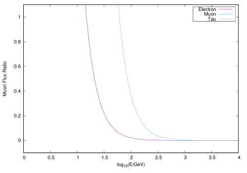
Figure 7: Final flux obtained from the extended source emission as a function of the neutrino energy.

Appendix B Description of the code

$\nu$-SQuIDS is a C++ code built using the SQuIDS framework [114]. It is designed to propagate neutrinos through media while taking into account flavor oscillations and non-coherent interactions.

In order to allow the user to compute simple oscillation probabilities for a single neutrino energy the code has a simplified mode. In this mode the neutrino energy is fixed and only coherent interactions are treated. In this case, only Eq. (5) is relevant for the neutrino propagation, and the nuSQuIDS class implements SQuIDS::H0 as in Eq. (7a) and SQuIDS::HI as given in Eq. (7b).

In the default mode a statistical ensemble of neutrinos is considered. The ensemble is described by means of a set of SU_vector objects located at fixed energy nodes spaced over the energy region under consideration. Besides defining SQuIDS::H0 and SQuIDS::HI, as in the simplified single energy mode, the following functions are also defined: SQuIDS::GammaRho by Eqs. (11a) and (11b), and SQuIDS::InteractionsRho in Eqs. (12a) and (12). Furthermore, in the latter Eq. (12) $\tau$-regeneration is implemented assuming instantaneous $\tau$ decay.

While the nuSQuIDS class implements all the necessary differential equations, one must also specify the neutrino propagation environment, propagation trajectory, and the relevant cross-sections. When interactions are considered the nuSQuIDS instance will automatically construct appropriate NeutrinoCrossSections and TauDecaySpectra objects to evaluate cross sections and $\tau$ physics respectively. However, the user can also replace these default versions if desired. The user must explicitly specify the neutrino propagation medium and trajectory through relevant specialization of Body and Body::Track. Several implementations of Body and Track covering common physics cases are supplied with the library.

Finally, nuSQuIDS provides a set of functions to evaluate the neutrino ensemble flavor and mass composition. The code also has the capability to store the system state in an HDF5 [165] file for later use.

B.1 Body & Track

Body and Body::Track are abstract C++ classes which are used to represent the environment in which neutrinos are propagated (Body) and the propagation path inside it (Body::Track). We will frequently use the shorthand Track for Body::Track, when it should be clear from context that this is the type of Track corresponding to a particular implementation of Body.

The evolution of the system depends on a single parameter which is a double member of Track. The interplay between the evolution of this parameter and the trajectory inside a given body is what is encoded in the Body and Body::Track classes. Namely, a Body is defined as a matter density and electron fraction depending on the position in a 3 dimensional space, $\rho_{m}(\vec{r})$ and $Y_{e}(\vec{r})$, the role of the Track would be equivalent to the trajectory ($\vec{r}(x)$) and the current position ($x$).

In the context of the code, the two main virtual functions that the user should provide in order to define a non-trivial Body are:

• ⬇

  virtual double density(std::shared_ptr<Track>);

  This function returns the density in ${\rm g}/{\rm cm}^{3}$ for a given Track position.

• ⬇

  virtual double ye(std::shared_ptr<Track>);

  Returns the electron fraction at a given Track position.

In order to allow the user to store the information of the object the following members are important,

• ⬇

  std::vector<double> BodyParams;

  Double vector that contains all the parameters that are needed to compute the density and electron fraction from the parameter x.

• ⬇

  bool is_constant_density = false;

  This variable is true if the density of the object is constant. This is used to set the fast computations internally.

Other public functions of the Body object are,

• ⬇

  virtual void Serialize(hid_t group) const=0;

  This is an abstract function whose argument is an HDF5 location where the user should store the body properties.

• ⬇

  static std::shared_ptr<Body> Deserialize(hid_t group);

  This is an abstract function whose argument is an HDF5 location with the body information to be used for the user to recover the body.

• ⬇

  unsigned int GetId() const {return 0;}

  It returns the Id of the body which is hard-coded by the user.

• ⬇

  std::string GetName() const {return name;}

  It returns the name of the object which is hard-coded by the user.

• ⬇

  const std::vector<double>& GetBodyParams() const

  { return BodyParams;}

  It returns a constant reference to the vector of parameters that define body.

• ⬇

  virtual bool IsConstantDensity() const

  {return is_constant_density;}

  It returns true if the body has constant density, false otherwise.

• ⬇

  virtual void SetIsConstantDensity(bool icd)

  {is_constant_density = icd;}

  Set true or false the constant density.

Furthermore, the Track object has the following protected variables, which are the initial, final and current evolution parameter values, by default in units of eV^-1

• ⬇

  double x;

  Current position.

• ⬇

  double xini;

  Initial position.

• ⬇

  double xend;

  Final position.

And the following public functions are provided,

• ⬇

  Track(double x,double xini, double xend):

  x(x), xini(xini),xend(xend) {}

  Constructor where we specify current, initial, and final positions.

• ⬇

  Track(double xini, double xend):

  Track(xini,xini,xend) {}

  Constructor where we specify initial and final positions. The current position is set to the initial.

• ⬇

  virtual void Serialize(hid_t group) const=0;

  This is an abstract function whose argument is an HDF5 location where the user should store the track properties.

• ⬇

  static std::shared_ptr<Body::Track> Deserialize(hid_t group);

  This is an abstract function whose argument is an HDF5 location with the track information to be used for the user to recover the track.

• ⬇

  void SetX(double y);

  Sets the current position along the trajectory.

• ⬇

  double GetX() const;

  Returns the current value of the evolution parameter x.

• ⬇

  double GetInitialX() const;

  Returns the initial value of the evolution parameter x.

• ⬇

  double GetFinalX() const;

  Returns the final value of the evolution parameter x

• ⬇

  static std::string GetName() {return "BodyTrack";};

  Returns the name of the track object hard-coded by the user.

• ⬇

  std::vector<double> GetTrackParams() const

  Returns a vector of doubles that define the trajectory.

• ⬇

  virtual void FillDerivedParams(std::vector<double>& TrackParams)

  const{};

  Should be implemented by derived classes to append their additional parameters to TrackParams

• ⬇

  void ReverseTrack()

  Interchanges initial and final positions.

Since Body and Track are abstract classes they themselves do not perform any task, but rather their specializations specify the real neutrino propagation environment and how it relates to its trajectory. $\nu$-SQuIDS implements the most commonly used environments and trajectory configurations. The user can create new classes in order to extend $\nu$-SQuIDS functionality.

The Body classes specializations implemented in $\nu$-SQuIDS are the following: Vacuum, ConstantDensity, VariableDensity, Earth, EarthAtm, Sun, and SunASnu.

In the following sub-sections we will describe the specific constructors and the functions that are not members of the parent class.

B.1.1 Vacuum

• Vacuum

  ⬇

  Vacuum():Body(){}

  Initializes a Vacuum environment.

• Vacuum::Track

  ⬇

  Track(double x,double xini,double xend):

  Body::Track(x,xini,xend){};

  Track(double xini,double xend):

  Track(xini,xini,xend){};

  Track(double xend):Track(0.0,xend){}

  Initialize the corresponding Track, setting the current (x), initial (xini), and final (xend) neutrino position in ${\rm eV}^{-1}$.

B.1.2 ConstantDensity

• ConstantDensity

  ⬇

  ConstantDensity(double density,double ye);

  Initializes a ConstantDensity environment with constant density (density in ${\rm g}/{\rm cm}^{3}$) and electron fraction (ye).

• ConstantDensity::Track

  ⬇

  Track(double x,double xini,double xend):

  Body::Track(x,xini,xend){};

  Track(double xini,double xend):

  Track(xini,xini,xend){};

  Track(double xend):Track(0.0,xend){}

  Initialize the corresponding Track, setting the current (x), initial (xini), and final (xend) neutrino position in ${\rm eV}^{-1}$.

B.1.3 VariableDensity

• VariableDensity

  ⬇

  VariableDensity(std::vector<double> x,

  std::vector<double> density,

  std::vector<double> ye);

  Initializes a VariableDensity environment given three equal size arrays specifying the density and electron fraction at given positions. An object will be created that interpolates using gsl_spline [166] along the x array to get the density and electron fraction as continuous functions.

• VariableDensity::Track

  ⬇

  Track(double x,double xini,double xend):

  Body::Track(x,xini,xend){};

  Track(double xini,double xend):

  Track(xini,xini,xend){};

  Track(double xend):Track(0.0,xend){}

  Initialize the corresponding Track, setting the current (x), initial (xini), and final (xend) neutrino position in ${\rm eV}^{-1}$.

B.1.4 Earth

The Earth body specification is designed to propagate neutrinos in the Earth from two points on the surface. Since the Earth in the PREM model is assumed to be spherically symmetric the length of the path is enough to determine the trajectory. AkimaSpline is used to interpolate $\rho$ and $y_{e}$ as a function of radius to the earth center.

• Earth

  ⬇

  Earth();

  Initializes an Earth environment as defined by the PREM [167].

  ⬇

  Earth(std::string earthmodel);

  Initializes an Earth environment as defined by a table given in the file specified by filepath. The table should have three columns: radius (where 0 is center and 1 is surface), density (${\rm g}/{\rm cm}^{3}$), and $y_{e}$ (dimensionless).

  ⬇

  Earth(std::vector<double> x,std::vector<double> rho,

  std::vector<double> ye);

  Initialize an earth whose radial density is specified by the values in the vector rho in ${\rm g}/{\rm cm}^{3}$, the electron fraction in the vector ye, and the radial positions in the vector x in centimeters.

  ⬇

  double GetRadius() const;

  Returns the radius of the Earth in eV^-1.

• Earth::Track

  ⬇

  Track(double x,double xini,double xend,double baseline):

  Body::Track(x,xini,xend),baseline(baseline){};

  Track(double xini,double xend,double baseline):

  Track(xini,xini,xend,baseline){};

  Initialize the corresponding Track setting the current (x), initial (xini), and final (xend) neutrino position in ${\rm eV}^{-1}$.

  ⬇

  Track(double baseline):Track(0.,baseline,baseline){}

  Constructor that sets the path in the earth for a given baseline baseline.

  ⬇

  double GetBaseline() const;

  Returns the baseline in eV^-1.

B.1.5 EarthAtm

This body includes both the density profile of the Earth and a simple model of its atmosphere. Paths end at the surface of the Earth, and are expressed in terms of their local zenith angle at the endpoint. The deafult atmosphere height is 22 km, and a scale height of 7.594 km is used for its density.

• EarthAtm

  ⬇

  EarthAtm();

  Initializes an Earth environment as defined by the PREM [167].

  ⬇

  EarthAtm(std::string earthmodel);

  Initializes an EarthAtm environment as defined by a table given in the file specified by filepath. The table should have three columns: relative radius (dimensionless, where 0 is the center and 1 the is surface), density (${\rm g}/{\rm cm}^{3}$), and electron fraction $y_{e}$ (dimensionless).

  ⬇

  EarthAtm(std::vector<double> x,std::vector<double> rho,

  std::vector<double> ye);

  Initialize an EarthAtm whose radial density is specified by the values in the vector rho in ${\rm g}/{\rm cm}^{3}$, the electron fraction in the vector ye, and the relative radial positions in the vector x.

  ⬇

  void SetAtmosphereHeight(double height);

  Change the height of the top of the atmosphere.

  ⬇

  EarthAtm::Track MakeTrack(double phi);

  Create a track which arrives at the surface with the given zenith angle and an initial position at the top of the atmosphere.

  ⬇

  EarthAtm::Track MakeTrackWithCosine(double cosphi);

  The same as MakeTrack, but takes the cosine of the zenith angle, which is a more convenient variable in many contexts.

• EarthAtm::Track

  ⬇

  Track(double x, double phi,

  double earth_radius, double atmheight);

  Track(double phi, double earth_radius, double atmheight);

  Initialize the corresponding Track by specifying the zenith angle in radians (phi), radius of the Earth (earth_radius) in eV^-1, height of the atmosphere (atmheight) in eV^-1, and the current position along the track (x) in eV^-1.

  ⬇

  double GetBaseline() const;

  Returns the baseline in eV^-1.

  ⬇

  static Track makeWithCosine(double cosphi,

  double earth_radius,

  double atmheight);

  Create a track with the cosine of the zenith angle (cosphi) instead of the angle.

B.1.6 Sun

This specification of the object allows to define the Sun and radial trajectories that start from the center of the sun.

• Sun

  ⬇

  Sun();

  Initializes a Sun environment as defined by the Standard Solar Model [168].

  ⬇

  Sun(std::vector<double> x,std::vector<double> rho,

  std::vector<double> xh);

  Initialize a Sun whose radial density is specified by the values in the vector rho in ${\rm g}/{\rm cm}^{3}$, the electron fraction in the vector ye, and the radial positions in the vector x in centimeters.

  ⬇

  Sun(std::string sunmodel);

  Initialize a Sun object from a text file that should have the same format as the Standard Solar Model [168]. Namely, the second column one must run from zero to one representing the center and surface of the Sun respectively. The fourth column must contain the Sun density in ${\rm g}/{\rm cm}^{3}$ at a given position, while the seven column must contain the hydrogen fraction, $r_{h}$, which is related to the electron fraction by $ye=0.5*(1.0+r_{h}(r))$. Internally we assume that the solar radius is 695980.0 kilometers.

• Sun::Track

  ⬇

  Sun::Track(double xend);

  This constructor sets the trajectory starting at the Sun center and ending at a distance xend from it.

• Sun::Track

  ⬇

  Sun::Track(double xini, double xend);

  Initialize the corresponding Track by the initial position in the sun xini and xend along the solar radius.

B.1.7 SunASnu

This specification of the object allows to define the Sun and the trajectories with different impact parameters.

• Sun

  ⬇

  SunASun();

  Initializes an Sun environment as defined by the Standard Solar Model [168].

  ⬇

  SunASnu(std::vector<double> x,std::vector<double> rho,

  std::vector<double> xh);

  Initialize an Sun whose radial density is specified by the values in the vector rho in ${\rm g}/{\rm cm}^{3}$, the electron fraction in the vector ye, and the radial positions in the vector x in centimeters.

  ⬇

  SunASnu(std::string sunmodel);

  Initialize a SunASnu object from a text file that should have the same format as the Standard Solar Model [168]. Namely, the second column one must run from zero to one representing the center and surface of the Sun respectively. The fourth column must contain the Sun density in ${\rm g}/{\rm cm}^{3}$ at a given position, while the seven column must contain the hydrogen fraction, $r_{h}$, which is related to the electron fraction by $ye=0.5*(1.0+r_{h}(r))$. Internally we assume that the solar radius is 695980.0 kilometers.

• SunASun::Track

  ⬇

  Track(double x,double xini,double b_impact);

  Track(double xini,double b_impact):Track(xini,xini,b_impact){};

  Track(double b_impact_):Track(0.0,b_impact_){}

  This constructor sets the trajectory starting at a distance xini, with current position x, and impact factor b_impact in eV^-1.

B.2 NeutrinoCrossSections

This object can be queried to obtain neutrino cross section information used when considering neutrino non-coherent interactions. The NeutrinoCrossSections is a base abstract class, which the user has to subclass and implement the relevant neutrino cross section for the problem at hand. The user must specify the total cross section per flavor and per interaction type (charge and neutral current), as well as the single differential cross sections with respect to the outgoing neutrino energy.

B.2.1 NeutrinoCrossSections

First, we define enumerations to label flavor, neutrino, and interaction type.

• NeutrinoFlavor

  ⬇

  enum NeutrinoFlavor

  {electron = 0, muon = 1, tau = 2, sterile = 3};

  Enumeration that is used to specify the neutrino flavor.

• NeutrinoType

  ⬇

  enum NeutrinoType {neutrino = 0, antineutrino = 1};

  Enumeration used to specify neutrino and antineutrino particle type.

• Current

  ⬇

  enum Current {CC, NC, GR};

  Enumeration used to specify charged (CC), neutral (NC) current interactions, and Glashow resonant interactions (GR).

Second we list the public abstract virtual functions.

• Total cross section

  ⬇

  virtual double TotalCrossSection(double Enu,

  NeutrinoFlavor flavor, NeutrinoType neutype,

  Current current) const;

  Abstract virtual function that given a neutrino energy (Enu) in eV, neutrino flavor (flavor), neutrino type (neutype), and interaction type (current) returns the total cross section in ${\rm cm}^{2}$.

• Single differential cross section

  ⬇

  virtual double SingleDifferentialCrossSection(double E1,

  double E2, NeutrinoFlavor flavor, NeutrinoType neutype,

  Current current) const;

  Abstract virtual function that given an incident neutrino energy (E1) in eV, outgoing neutrino energy (E2) in eV, neutrino flavor (flavor), neutrino type (neutype), and interaction type (current) returns the differential cross section with respect to the outgoing neutrino energy in ${\rm cm}^{2}{\rm GeV}^{-1}$.

• Double differential cross section

  ⬇

  virtual double DoubleDifferentialCrossSection(double E,

  double x, double y,NeutrinoFlavor flavor,

  NeutrinoType neutype, Current current) const;

  Virtual function such that given the neutrino energy (E), Bjorken-x (x), and y (y) should return the double differential cross section. Its implementation is not required to run nuSQUIDS and, by default, when evaluated, unless overwritten, it will throw an error.

• Averaged cross sections

  ⬇

  virtual double AverageTotalCrossSection(double EMin,

  double EMax, NeutrinoFlavor flavor, NeutrinoType neutype,

  Current current) const;

  virtual double AverageSingleDifferentialCrossSection(double E1,

  double E2Min, double E2Max, NeutrinoFlavor flavor,

  NeutrinoType neutype, Current current) const;

  Averaged total and single differential cross section in energy range Emin-Emax and E2min-E2max respectively.

B.2.2 NullCrossSections

This class is a simple implementation of the a null cross section.

⬇

NullCrossSections(){}

double TotalCrossSection(double Enu, NeutrinoFlavor flavor,

NeutrinoType neutype, Current current) const override { return 0;}

double SingleDifferentialCrossSection(double E1, double E2,

NeutrinoFlavor flavor, NeutrinoType neutype, Current current)

const override { return 0;}

double DoubleDifferentialCrossSection(double E, double x, double y,

NeutrinoFlavor flavor, NeutrinoType neutype, Current current)

const override { return 0;}

B.2.3 NeutrinoDISCrossSectionsFromTables

This class uses pre-calculated deep inelastic scattering (DIS) cross section tables which are provided by nuSQuIDS or by the user. In the code two different cross sections are available by default: csms.h5 is a perturbative QCD next-to-leading order calculation [128] using the HERA parton distribution functions [169], recalculated for proton and neutron targets, and updated to account for the non-zero mass of the tau, reducing the $\nu_{\tau}$ cross sections at low energies compared to the originally published version. nusigma [170] is a first order QCD calculation using the CTEQ6 parton distribution functions on an iso-scalar target. In the csms calculation the mass of the tau is neglected, thus the neutrinos cross section is the same for all flavors; this is not the case for the nusigma calculation. Both correspond to deep inelastic scattering which is the dominant neutrino interaction with nucleons above $O({\rm 10~{}GeV})$.

The cross sections are loaded from tables included in nuSQUIDS/data/xsections/, or provided by the user. The cross section object can be constructed from a single HDF5 file that contains both single and total cross sections or by a set of twelve text files, containing all cross sections related to a single target species (e.g. all cross sections for DIS neutrino interactions with protons).

When an HDF5 file is used, it must have an internal structure as shown in Table 8. All cross sections must be tabulated with the same set of incident neutrino energies, and each singly-differential cross section must be tabulated for the same set of out-going lepton energies, expressed in the $z$ variable described in Sec. D. These common energy and $z$ values are stored in the one-dimensional energies and zs datasets. For the energies, more specifically, the base-10 logarithms of the energies in GeV are stored. All total cross section tables are one-dimensional datasets containing the base-10 logarithm of the cross section values in cm², and all singly-differential cross section tables are two-dimensional datasets with dimensions incident and out-going energy containing the base-10 logarithm of the cross section values in cm².

When text files are used, they must be organized into three groups, one for each active neutrino flavor, with a corresponding filename component (electron_, muon_, or tau_). The four text files within each flavor set must end with the suffixes nu_dsde_CC.dat, nubar_dsde_NC.dat, nu_sigma_CC.dat, and nubar_sigma_NC.dat for the singly differential neutrino, singly differential antineutrino, total neutrino, and total antineutrino cross sections, respectively. Each total cross section file must contain two columns: The incident neutrino energy in GeV and the total cross section in cm². Each singly-differential cross section file must have three columns: The incident neutrino energy in GeV, outgoing neutrino energy encoded via the unitless $z$ variable described in the next section, and the differential cross section in cm².

Figure 8: HDF5 cross section format. ‘CC’ and ‘NC’ are abbreviations for charged-current and neutral current, respectively. For the common case that two flavors (e.g. electron and muon) have indistinguishable cross section values, one group may be a link to the other within the file.

B.2.4 Constructors

• Default constructor.

  ⬇

  NeutrinoDISCrossSectionsFromTables();

  This constructor load the defaults csms.h5 file

The files to load the different cross-sections can be specified explicitly as follows.

⬇

NeutrinoDISCrossSectionsFromTables csh5(’./csms.h5’);

NeutrinoDISCrossSectionsFromTables cstxt(’./nusigma_’);

B.2.5 Functions

• Total cross sections

  ⬇

  double TotalCrossSection(double Enu,

  NeutrinoFlavor flavor, NeutrinoType neutype,

  Current current) const;

  Returns the total cross section at an energy Enu in eV, neutrino flavor flavor, neutrino type neutype, and current can be either NC or CC for neutral or charge current DIS cross sections. This function performs a linear interpolation in the logarithm of the neutrino energy to estimate the cross section from a reference table.

• Single differential cross sections

  ⬇

  double SingleDifferentialCrossSection(double E1, double E2,

  NeutrinoFlavor flavor, NeutrinoType neutype,

  Current current) const;

  Function that given an incident neutrino energy (E1) in eV an outgoing lepton energy (E2), as well as neutrino flavor, type, and process, returns the differential cross section with respect to the outgoing lepton energy in ${\rm cm}^{2}/{\rm GeV}$. This function interpolates the cross section from a reference table by means of a bi-linear interpolation.

B.2.6 GlashowResonanceCrossSection

This class implements the formulas in [102] in order to calculate the electron antineutrino Glashow resonance cross section contribution.

B.2.7 Constructors

• Default constructor.

  ⬇

  GlashowResonanceCrossSection();

B.2.8 Functions

• Total cross sections

  ⬇

  double TotalCrossSection(double Enu,

  NeutrinoFlavor flavor, NeutrinoType neutype,

  Current current) const;

  Returns the total cross section in cm² at an energy Enu in eV, neutrino flavor flavor, and neutrino type neutype. If the flavor is not electron and neutrino type is not antineutrino it returns zero.

• Single differential cross section

  ⬇

  double SingleDifferentialCrossSection(double E1, double E2,

  NeutrinoFlavor flavor, NeutrinoType neutype,

  Current current) const;

  Returns the single differential cross section in cm²/GeV for an incident neutrino energy (E1) in eV an outgoing neutrino energy (E2) in eV, neutrino flavor (flavor), and neutrino type (neutype). If the flavor is not electron and neutrino type is not antineutrino it returns zero.

B.3 TauDecaySpectra

This object can be queried to obtain $\tau$ decay physics into leptons and hadrons. The formulas implemented in this class were taken from [129]. It is only used when $\tau$-regeneration is activated and it returns the following quantities on the energy nodes,

$$\frac{dN^{lep/had}_{dec}(E_{\tau},E_{\nu})}{dE_{\nu}}{\rm~{}~{}and~{}~{}}\frac{d\bar{N}^{lep/had}_{dec}(E_{\tau},E_{\nu})}{dE_{\nu}},$$ (20)

i.e. the neutrino and antineutrino spectral distributions from $\tau$ leptonic and hadronic decay modes.

B.3.1 Constructors and Initializing Functions

• Default constructor.

  ⬇

  TauDecaySpectra();

• Constructor and initializing function with memory reservation.

  ⬇

  TauDecaySpectra(marray<double,1> E_range);

  void Init(marray<double,1> E_range);

  This constructor and initialization function calculates and stores the $\tau$ decay spectra on nodes specified by the one dimensional array E_range in eV.

B.3.2 Functions

The following functions assume that the $\tau$ and $\bar{\tau}$ have the same decay distribution.

• (Anti)Neutrino spectra with respect to neutrino energy.

  ⬇

  double dNdEnu_All(int e1,int e2) const;

  Returns neutrino decay spectra evaluated from energy node e1 to energy node e2 when $\tau$ decays into leptons or hadrons.

  ⬇

  double dNdEnu_Lep(int e1,int e2) const;

  Returns neutrino decay spectra evaluated between energy nodes e1 and e2 when $\tau$ decays into leptons.

• (Anti)Neutrino spectra with respect to $\tau$ energy.

  ⬇

  double dNdEle_All(int e1,int e2) const;

  Returns neutrino decay spectra evaluated between energy nodes e1 and e2 when $\tau$ decays into leptons or hadrons with respect to the initial $\tau$ energy.

  ⬇

  double dNdEle_Lep(int e1,int e2) const;

  Returns neutrino decay spectra evaluated between energy nodes e1 and e2 when $\tau$ decays into leptons with respect to the initial $\tau$ energy.

• Get the $\tau$ branching ratio to leptons.

  ⬇

  double GetTauToLeptonBranchingRatio() const;

  Returns the $\tau$ branching ratio to leptons.

• Get the $\tau$ branching ratio to hadrons.

  ⬇

  double GetTauToHadronBranchingRatio() const;

  Returns the $\tau$ branching ratio to hadrons.

B.4 nuSQUIDS

This object is a specialization of the SQUIDS class [114] that implements the differential equations as described in Sec. 2. In particular, it is used to specify the propagation Body and its associated Track. Moreover, it uses the NeutrinoCrossSections and TauDecaySpectra in order to evaluate the neutrino cross sections and $\tau$ decay spectra; the latter is only used when $\tau$ regeneration is enabled. Furthermore, it enables the user to modify the neutrino oscillation parameters as well as the differential equation numerical precision. Finally, it also has the capability to create and read HDF5 files that store the program results and configuration.

B.4.1 Constructors

• Default constructor.

  ⬇

  nuSQUIDS();

• Move constructor.

  ⬇

  nuSQUIDS(nuSQUIDS&&);

  Constructs a nuSQUIDS object from an r-value reference.

• Single energy mode constructor.

  ⬇

  nuSQUIDS(unsigned int numneu, NeutrinoType NT);

  This constructor and initialization function initializes nuSQUIDS in the single energy mode. numneu specifies the number of neutrino flavors which can go from two to six, while NT can be set to neutrino or antineutrino.

• Multiple energy mode constructor.

  ⬇

  nuSQUIDS(marray<double,1> E_vector,

  unsigned int numneu,NeutrinoType NT = both,

  bool iinteraction = false,

  std::shared_ptr<NeutrinoCrossSections> ncs = nullptr)

  This constructor and initialization function initializes nuSQUIDS in the multiple energy mode. We need to provide the following arguments: list of neutrino energy nodes (E_vector), number of neutrino flavors (numneu), neutrino or anti-neutrino type (NT), non-coherent scattering interactions (iinteraction), and neutrino cross section object pointer (ncs).

• Constructing from a $\nu$SQuIDS-HDF5 file

  ⬇

  nuSQUIDS(std::string hdf5_filename, std::string grp = "/",

  std::shared_ptr<InteractionStructure> int_struct = nullptr)

  This constructor initializes nuSQUIDS from a previously generated $\nu$SQuIDS HDF5 file. filepath must specify the full path of the HDF5 file, grp specifies the location on the HDF5 file structure where the object will be saved (by default it will be saved on the root of the HDF5 file), and int_struct can specify the cross-section object instead of loading it from the file.

B.4.2 Functions

Functions to evaluate flavor and mass composition

• Flavor composition evaluator (single energy mode)

  ⬇

  double EvalFlavor(unsigned int flv) const;

  Returns the content of a given neutrino flavor specified by flv (0 = $e$, 1 = $\mu$, 2 = $\tau$, …). This function can only be used in the single energy mode.

• Flavor composition evaluator (multiple energy mode)

  ⬇

  double EvalFlavorAtNode(unsigned int flv, unsigned int ie,

  unsigned int rho=0) const;

  double EvalFlavor(unsigned int flv, double enu,

  unsigned int rho=0) const;

  double EvalFlavor(unsigned int flv,double enu,

  unsigned int rho,double scale,

  std::vector<bool>& avr) const;

  EvalFlavorAtNode returns the content of a given neutrino flavor specified by flv (0 = $e$, 1 = $\mu$, 2 = $\tau$, ...) at an energy node ie. Furthermore, EvalFlavor returns the approximate content of a given flavor for a specific neutrino energy enu by interpolating in the interaction basis. In each function, when considering NT = both, the parameter rho toggles between neutrino (0) and antineutrino (1). The last overload takes two additional arguments: a scale, such that all $H_{0}$ induced oscillation frequencies larger than this scale will be averaged, and a vector of booleans, which entries will be set to true if the corresponding oscillations frequencies have been averaged out.

• Mass composition evaluator (single energy mode)

  ⬇

  double EvalMass(unsigned int eig) const;

  Returns the content of a given neutrino mass eigenstate specified by eig (0 = $\nu_{1}$, 1 = $\nu_{2}$, 2 = $\nu_{3}$, ...). This function can only be used in the single energy mode.

• Mass composition evaluator (multiple energy mode)

  ⬇

  double EvalMassAtNode(unsigned int eig, unsigned int ie,

  unsigned int rho=0) const;

  double EvalMass(unsigned int eig, double enu,

  unsigned int rho=0) const;

  double EvalMass(unsigned int flv,double enu,

  unsigned int rho,double scale,

  std::vector<bool>& avr) const;

  EvalMassAtNode returns the content of a given neutrino mass eigenstate specified by eig (0 = $\nu_{1}$, 1 = $\nu_{2}$, 2 = $\nu_{3}$, ...) at an energy node ie. Furthermore, EvalMass returns the approximate content of a given mass eigenstate for a specific neutrino energy enu by interpolating in the interaction basis. In each function, when considering NT = both, the parameter rho toggles between neutrino (0) and antineutrino (1). The last function gets two additional arguments: a scale, such that all $H_{0}$ induced oscillation frequencies larger than this scale will be averaged, and a vector of booleans, which entries will be set to true if the corresponding oscillations frequencies have been averaged out.

Functions to evolve the neutrino ensemble

• Evolve state

  ⬇

  void EvolveState();

  Once the neutrino propagation problem has been set up, this function evolves the neutrino state from its initial position to its final position specified by the track.

Functions obtain properties of the nuSQUIDS object as well as the state

• Get energy nodes values

  ⬇

  marray<double,1> GetERange() const;

  Returns a one-dimensional array containing the energy nodes positions given in eV.

• Get number of energy nodes

  ⬇

  unsigned int GetNumE() const;

  Returns the number of energy nodes.

• Get number of neutrino flavors

  ⬇

  unsigned int GetNumNeu() const;

  Returns the number of neutrino flavors.

• Get Hamiltonian at current position

  ⬇

  SU_vector GetHamiltonian(unsigned int ie,

  unsigned int rho = 0);

  Returns the SU_vector that represents the (anti)neutrino Hamiltonian at the current position, at a given energy node ie, and rho specifies whether the neutrino or antineutrino hamiltonian is returned.

• Get the state of the system

  ⬇

  const squids::SU_vector& GetState(unsigned int ei,

  unsigned int rho = 0) const;

  Returns the SU_vector that represents the (anti)neutrino state at given energy node ie, and rho specifies whether the neutrino or antineutrino state is returned.

• Get the flavor projector

  ⬇

  SU_vector GetFlavorProj(unsigned int ie,

  unsigned int rho = 0) const;

  Returns an SU_vector that represents the flavor projector for the energy node ie, and rho specifies if neutrinos or antineutrinos are requested.

• Get the mass projector

  ⬇

  SU_vector GetMassProj(unsigned int ie,

  unsigned int rho = 0) const;

  Returns an SU_vector that represents the mass projector for the energy node ie, and rho specifies if neutrinos or antineutrinos are requested.

• Get Body

  ⬇

  std::shared_ptr<Body> GetBody() const;

  Returns the Body instance currently stored in the nuSQUIDS object.

• Get Track

  ⬇

  std::shared_ptr<Track> GetTrack() const;

  Returns the Track instance currently stored in the nuSQUIDS object.

• Get mixing angle

  ⬇

  double Get_MixingAngle(unsigned int i, unsigned int j) const;

  Returns the $\theta_{i,j}$ mixing angle where i and j are zero based indices.

• Get CP phase

  ⬇

  double Get_CPPhase(unsigned int i, unsigned int j) const;

  Returns the $\delta_{i,j}$ $CP$ phase where i and j are zero based indices.

• Get square mass difference

  ⬇

  double Get_SquareMassDifference(unsigned int i) const;

  Returns the $\Delta m^{2}_{i0}$ in ${\rm eV}^{2}$ where $1\leq i<{\rm\tt numneu}$.

Functions to set properties of the nuSQUIDS object as well as the state

• Set Body

  ⬇

  void Set_Body(std::shared_ptr<Body>);

  Sets the Body instance in which the neutrino propagation will take place.

• Set Track

  ⬇

  void Set_Track(std::shared_ptr<Track>);

  Sets the Track instance which describes the neutrino propagation inside a given Body.

• Set the initial state

  ⬇

  void Set_initial_state(marray<double,1> state, Basis basis);

  void Set_initial_state(marray<double,2> state, Basis basis);

  void Set_initial_state(marray<double,3> state, Basis basis);

  Set_initial_state sets the initial neutrino (and antineutrino) state. The states can be specified for the single and multiple energy modes using the appropiate C++ signature. In each case basis can be either mass or flavor.

  • marray<double,1> state: Can only be used in single energy mode and is defined by state[$\alpha$] = $\phi_{\alpha}$ where $\alpha$ is a flavor or mass eigenstate index.

  • marray<double,2> state: Can only be used in multiple energy mode and is defined by state[ei][$\alpha$] = $\phi_{\alpha}(E$[ei]$),$ i.e. the flavor (mass) eigenstate composition at a given energy node ei.

  • marray<double,3> state: Can only be used in multiple energy mode and is defined by state[ei][$\rho$][$\alpha$] = $\phi^{\rho}_{\alpha}(E$[ei]$),$ i.e. the flavor (mass) eigenstate composition at a given energy node ei, and where $\rho=0\equiv{\rm neutrino}$ and $\rho=1\equiv{\rm antineutrino}$.

• Set energy

  ⬇

  void Set_E(double enu);

  Set the neutrino energy. This function can only be used in the single energy mode and enu has to be in natural units.

• Enable progress bar

  ⬇

  void Set_ProgressBar(bool opt);

  If opt is true a progress bar will be printed to indicate the calculation progress.

• Enable tau regeneration

  ⬇

  void Set_TauRegeneration(bool opt);

  If opt is true, NT is both, and non-coherent interactions are enabled, tau regeneration effects will be included.

• Set mixing angle

  ⬇

  void Set_MixingAngle(unsigned int i, unsigned int j,

  double angle);

  Sets the $\theta_{i,j}$ mixing angle to angle, where i and j are zero-based indexes, and angle must be given in radians.

• Set CP phase

  ⬇

  void Set_CPPhase(unsigned int i, unsigned int j,

  double phase);

  Sets the $\delta_{i,j}$ $CP$ phase to phase, where i and j are zero-based indexes, and phase must be given in radians.

• Set square mass difference

  ⬇

  void Set_SquareMassDifference(unsigned int i, doble dmsq);

  Sets the $\Delta m^{2}_{i0}$ to dams, given in ${\rm eV}^{2}$, where $1\leq i<{\rm\tt numneu}$.

• Set parameters to default

  ⬇

  void Set_MixingParametersToDefault();

  Sets the mixing angles and square mass mixings to the best fit point given in [171].

• Set the basis of solution

  ⬇

  void Set_Basis(Basis basis);

  Sets the basis in which the evolution will be performed. Two options are available: mass and interaction, the latter being the default.

• Set neutrino cross-section

  ⬇

  void SetNeutrinoCrossSections(

  std::shared_ptr<NeutrinoCrossSections> xs)

  Sets the neutrino cross-section B.2 given by the shared pointer xs to the nuSQuIDS object.

HDF5 interface functions

• Write nuSQUIDS object into an HDF5 file.

  ⬇

  void WriteStateHDF5(std::string hdf5_filename,

  std::string group = "/",

  bool save_cross_sections = true,

  std::string cross_section_grp_loc = "")

  const;

  Writes the current nuSQUIDS configuration and state into an HDF5 file for later use. hdf5_filename specifies the output filename, group is the location in the HDF5 structure where the nuSQUIDS object will be saved; by default the root of the HDF5 will be used. Furthermore, save_cross_sections and cross_section_grp_loc specify if and where in the HDF5 file structure will the cross sections be saved, respectively See Figure 9 for details of the nuSQUIDS HDF5 structure.

• Add to the HDF5 write funtion.

  ⬇

  virtual void AddToWriteStateHDF5(hid_t hdf5_loc_id) const;

  Enables the user to add content to the HDF5 file. An HDF5 location identifier,hdf5_loc_id, will be provided by nuSQUIDS. Using this identifier the user can store relevant information about the derived nuSQuIDS class.

• Read nuSQUIDS object from an HDF5 file.

  ⬇

  void ReadStateHDF5(std::string hdf5_filename,

  std::string group = "/",

  std::string cross_section_grp_loc = "");

  Reads a previously generated HDF5 file and sets the nuSQUIDS object accordingly, i.e. it configures it and loads the saved state. hdf5_filename specifies the input filename, group is the location in the HDF5 structure where the nuSQUIDS object is; by default the root of the HDF5 is assumed. Furthermore, cross_section_grp_loc specify where the cross sections are in the HDF5 file structure. See Figure 9.

• Add to the HDF5 read file.

  ⬇

  virtual void AddToReadStateHDF5(hid_t hdf5_loc_id);

  Enables the user to read user defined content from the HDF5 file. An HDF5 location,hdf5_loc_id, is provided so the user can interface with the HDF5 library. For a correct implementation this functions has to be written consistently with the AddToWriteStateHDF5 function.

Figure 9: Structure of nuSQUIDS HDF5 file. The crosssections group will only be written when interactions are enabled. Furthermore, user_parameters is by default empty and can be set/accessed by AddToWriteStateHDF5/AddToReadStateHDF5.

B.5 nuSQUIDSAtm

Atmospheric neutrino oscillations are a major and instrumental part of research in contemporary neutrino physics. Experiments like SuperKamiokande, IceCube, and Antares have used atmospheric neutrinos to measure neutrino mass splittings and mixing angles. Furthermore, proposed extensions like HyperKamiokande, PINGU, and ORCA ought to improve the current measurements and have sensitivity to neutrino mass ordering. This class allows to propagate a set of full energy spectrum of neutrinos for different zenith angles. It implements functions to easily set the initial conditions and also interpolations of the fluxes.

B.5.1 Constructors

• Constructor with costh range.

  ⬇

  template<typename... ArgTypes> nuSQUIDSAtm(

  marray<double,1> costh_array, ArgTypes&&... args)

  This constructor creates a set of nuSQUIDS or derived nuSQUIDS objects with a set of zenith angles given by the marray costh_array. The arguments given in arg are the corresponding arguments of the nuSQUIDS or derived nuSQUIDS class constructor.

• Constructing from a nuSQuIDSAtm-HDF5 file

  ⬇

  nuSQUIDSAtm(std::string hdf5_filename)

  This constructor initializes nuSQUIDS from a previously generated $\nu$SQuIDS-HDF5 file. The resulting nuSQUIDS object will be given in single or multiple energy mode depending on the HDF5 file configuration. filepath must specify the full path of the HDF5 file. Furthermore, grp specifies the location in the HDF5 file structure where the object will be saved; by default it will be saved on the root of the HDF5 file.

• Move constructor.

  ⬇

  nuSQUIDSAtm(nuSQUIDSAtm&&);

  B.5.2 Functions

• Set initial state.

  ⬇

  void Set_initial_state(const marray<double,3>& ini_flux,

  Basis basis=flavor);

  void Set_initial_state(const marray<double,4>& ini_flux,

  Basis basis=flavor);

  Sets the initial state of the system given in the marray ini_flux, basis is the basis in which the state is defined. Different marray can be used for different cases:

  • marray<double,3> state: Can only be used in multiple energy mode and is defined by state[czi][ei][$\alpha$] = $\phi_{\alpha}(E$[ei]$,costh$[czi]$),$ i.e. the flavor (mass) eigenstate composition at a given energy and cosine zenith node ei and czi.

  • marray<double,4> state: Can only be used in multiple energy mode and is defined by state[czi][ei][$\rho$][$\alpha$] = $\phi^{\rho}_{\alpha}(E$[ei]$,costh$[czi]$),$ i.e. the flavor (mass) eigenstate composition at a given energy and zenith node ei and czi, and where $\rho=0\equiv{\rm neutrino}$ and $\rho=1\equiv{\rm antineutrino}$.

• Evolve function

  ⬇

  void EvolveState();

  Function that evolves the system.

• Evaluate the flux for a given flavor.

  ⬇

  double EvalFlavor(unsigned int flv,double costh,

  double enu, unsigned int rho,

  double scale,std::vector<bool> avr) const;

  double EvalFlavor(unsigned int flv,double costh,

  double enu,unsigned int rho = 0,

  bool randomize_production_height = false) const;

  It returns the flux for the flavor flv at the value of cosine zenith given by costh and energy given by enu. rho is neutrino or antineutrino. Some arguments can also be set: If a frequency is higher than scale it will be averaged out, and the corresponding entry in the Boolean vector avr will be set to true. In the second case the randomization of the production height of the neutrino can be set to $true$, by default is $false$.

• Read and write function.

  ⬇

  void ReadStateHDF5(std::string hdf5_filename);

  void WriteStateHDF5(std::string hdf5_filename,

  bool overwrite = true) const;

  These functions read and write the state of the system in the file hdf5_filename, in WriteStateHDF5 overwrite may be set to true or false.

• Set functions as in nuSQUIDS.

  ⬇

  void Set_MixingParametersToDefault();

  void Set_MixingAngle(unsigned int i,

  unsigned int j,double angle);

  void Set_CPPhase(unsigned int i,

  unsigned int j,double angle);

  void Set_SquareMassDifference(unsigned int i,double sq);

  void Set_h(double h);

  void Set_h_max(double h);

  void Set_h_min(double h);

  void Set_abs_error(double eps);

  void Set_rel_error(double eps);

  void Set_GSL_step(gsl_odeiv2_step_type const * opt);

  void Set_ProgressBar(bool opt);

  void Set_TauRegeneration(bool opt);

  void Set_GlashowResonance(bool opt);

  void Set_IncludeOscillations(bool opt);

  void Set_AllowConstantDensityOscillationOnlyEvolution(bool opt);

  void Set_PositivityConstrain(bool opt);

  void Set_PositivityConstrainStep(double step);

  void SetNeutrinoCrossSections(

  std::shared_ptr<NeutrinoCrossSections> xs);

  All these functions do a recursive call to the function with the same name in all the nuSQUIDS objects.

• Set earth model.

  ⬇

  void Set_EarthModel(std::shared_ptr<EarthAtm> earth);

  Sets the body given by earth to all the nuSQUIDS objects in every node.

• Sets the number of threads

  ⬇

  void Set_EvalThreads(unsigned int nThreads);

  The evolution can be done in a multi-thread with the number of threads specified by nThreads.

• Set absolute error in a given node.

  ⬇

  void Set_abs_error(double eps, unsigned int idx);

  Sets the GSL absolute error in the cosine zenith node given by $idx$.

• Number of threads.

  ⬇

  unsigned int Get_EvalThreads() const{

  Returns the number of threads used in the evaluation.

• Get mixing angles.

  ⬇

  double Get_MixingAngle(unsigned int i, unsigned int j) const;

  Returns the mixing angle of the first cosine zenith node in the rotation plane given by (i, j).

• Get square mass difference.

  ⬇

  double Get_SquareMassDifference(unsigned int i) const;

  Returns the square mass difference value given by i.

• Number of energy nodes.

  ⬇

  size_t GetNumE() const;

  Gives the number of energy nodes.

• Number of cosine zenith nodes.

  ⬇

  size_t GetNumCos() const;

  Gives the number of cosine zenith nodes.

• Number of rho.

  ⬇

  unsigned int GetNumRho() const;

  Gives the number of rho, for neutrino-antineutrino case it will be two.

• Energy array.

  ⬇

  marray<double,1> GetERange() const;

  Returns an marray with the value of the energies in the energy nodes.

• Cosine zenith array.

  ⬇

  marray<double,1> GetCosthRange() const;

  Returns an marray with the value of the cosine zenith in the cosine zenith nodes.

• Get the nuSQUIDS object.

  ⬇

  BaseSQUIDS& GetnuSQuIDS(unsigned int ci);

  Returns the nuSQUIDS object in the cosine zenith node ci.

• Get the array of nuSQUIDS.

  ⬇

  std::vector<BaseSQUIDS>& GetnuSQuIDS();

  Returns a std::vector with the nuSQUIDS objects in all the cosine zenith nodes.

Appendix C Python Interface

As the particle physics community has transitioned from FORTRAN to C++ based frameworks, it is also a current trend to be able to interface analysis software with high-level interpreted languages such as Mathematica, R, and Python. Of these languages we have decided to implement bindings with Python due to the well-developed C++-Python bindings given by the Boost library.

C.1 Installation

In order to install nuSQuIDS python bindings, additional libraries are required, namely, Boost.Python ($\geq 1.54$) and Python.numpy ($\geq 1.7$). Upon installing these new prerequisites you can run the following command to generate a Makefile to compile the bindings

⬇

./configure --with-python-bindings

This command will try to autodetect the location of the aforementioned mentioned libraries. The following configuration script flags are influencial and can be used to set pre-requisites locations:

• Specify the Python executable

  ⬇

  --python-bin=PYTHON_EXECUTABLE

  The provided Python executable will be used to find the python version, libraries, and includes.

• Set Boost library and include paths

  ⬇

  --with-boost=DIR

  --with-boost-incdir=DIR

  --with-boost-libdir=DIR

  The incdir and libdir options are used to set the boost include and library directories. The first option is a convenient flag that sets both directories to: DIR/lib and DIR/include for the library and include directory.

This will produce a Makefile in the resources/python/src directory of nuSQuIDS. This Makefile will be compiled when you run make on the main nuSQuIDS folder. This will produce a shared library in resources/python/pybindings; in order to be able to use the python bindings you need to add this directory to the system variable PYTHONPATH. For example, in the Bash shell

⬇

export PYTHONPATH=NUSQUIDS_DIR/resources/python/bindings:$PYTHONPATH

After successful installation you can import the python bindings in the following manner

⬇

import nuSQUIDSpy as nsq

where here we have introduced the alias nsq for the nuSQuIDS python module. We can further extend the capabilities of nuSQuIDS in Python by means of the the nuSQUIDSTools module. When it is loaded the nuSQuIDS functions and objects get overloaded with additional functionalities. In order to enable them, after loading the nuSQUIDSpy module, do

⬇

import nuSQUIDSTools

C.2 Description of the interface

The interface is implemented in two files nuSQUIDSpy.h and nuSQUIDSpy.cpp. Additionally in resources/python/inc the file container_conversions.h is provided to enable translation between std::vector<type> to List among C++ and Python. The python bindings header contains C++ templates that facilitate registration of nuSQuIDS python bindings.

In the bindings source file the following classes have been registered:

• nuSQUIDS,

• nuSQUIDSAtm,

• NeutrinoCrossSections,

• NullCrossSections,

• NeutrinoDISCrossSectionsFromTables,

• TauDecaySpectra,

• Body, Body.Track

• ConstantDensity, ConstantDensity.Track

• VariableDensity, VariableDensity.Track

• Earth, Earth.Track

• Sun, Sun.Track

• SunASnu, SunASnu.Track

• EarthAtm, EarhAtm.Track

for all these classes we have implemented the public members described in this document with the same names as in the C++ interface. Additionally, two classes from SQuIDS have been exposed to Python:

• SU_vector and

• Const.

See [114] for details on these classes. Also, the following enumerations have been made available in Python

• GSL_STEP_FUNCTIONS enumeration contains the following members:

  • GSL_STEP_RK2,

  • GSL_STEP_RK4,

  • GSL_STEP_RKF45,

  • GSL_STEP_RKCK,

  • GSL_STEP_RK8PD,

  • and GSL_STEP_MSADAMS.

  These can be used in the Set_GSL_step nuSQUIDS member function.

• Basis, which contains the members:

  • mass (Basis::mass),

  • flavor (Basis::flavor),

  • and interaction (Basis::interaction).

• NeutrinoCrossSections_NeutrinoFlavor, which contains the members:

  • electron (NeutrinoCrossSections::NeutrinoFlavor::electron),

  • muon (NeutrinoCrossSections::NeutrinoFlavor::muon),

  • tau (NeutrinoCrossSections::NeutrinoFlavor::tau),

  • and sterile (NeutrinoCrossSections::NeutrinoFlavor::sterile).

• NeutrinoCrossSections_NeutrinoType, which contains the members:

  • neutrino (NeutrinoCrossSections::NeutrinoType::neutrino)

  • and antineutrino (NeutrinoCrossSections::NeutrinoType::antineutrino).

• NeutrinoCrossSections_Current, which contains the members:

  • CC (NeutrinoCrossSections::Current::CC),

  • NC (NeutrinoCrossSections::Current::NC),

  • and GR (NeutrinoCrossSections::Current::GR).

• Neutrinotype, which contains the members:

  • neutrino (NeutrinoType::neutrino),

  • antineutrino (NeutrinoType::antineutrino),

  • and both (NeutrinoType::both).

Finally, conversion between Numpy.Array and marray<double,DIM> has been made available up to dimension four. Higher dimensionality multidimensional array conversion is possible by adding the following lines to the boost python module

⬇

to_python_converted< marray<double, DIM>, marray_to_numpyarray<DIM> >();

marray_from_python<DIM>();

where DIM is the array dimensionality to register.

C.3 Python walk-through

In this section we will illustrate the usage of the Python interface. These examples can be found in the IPython notebook located in resources/python/example. We start by importing the modules

⬇

1import numpy as np

2import matplotlib.pyplot as plt

3import nuSQUIDSpy as nsq

4import nuSQUIDSTools

Throughout the example we will use the shorthand nsq for the nuSQUIDS python bindings.

C.3.1 Single-energy mode

To start, like in the C++ case, we need to create a $\nu$-SQuIDS object. To begin this demonstration we will create a simple single-energy mode three-flavor neutrino oscillation calculator. Thus we just need to specify the number of neutrinos (3) and if we are dealing with neutrinos or antineutrinos.

⬇

nuSQ = nsq.nuSQUIDS(3,nsq.NeutrinoType.neutrino)

<<<<<<< HEAD

nuSQuIDS inputs should be given in natural units. In order to make this convenient, as in the C++ code, we make use of the SQuIDS class Const. We can instantiate it as follows

⬇

units = nsq.Const()

As in the C++ $\nu$-SQuIDS interface one can propagate the neutrinos in various environments (see A.4 for further details). We can start by considering oscillactions in vacuum by setting:

⬇

nuSQ.Set_Body(nsq.Vacuum())

Since we have to specify that we are considering vacuum propagation, we must construct a trajectory inside that object. This can be done using the Track class-property of a given Body. Each Body will have its own Track subclass and its constructors. We can set and construct a vacuum trajectory in the following way:

⬇

nuSQ.Set_Track(nsq.Vacuum.Track(100.0*units.km))

Next we have to set the neutrino energy, which can be done as follows

⬇

nuSQ.Set_E(1.0*units.GeV)

Now we have to set the initial neutrino state. We can provide this state in either the flavor or mass basis. We can do this using the Set_initial_state function, providing it with a numpy array and a nsq.Basis. If the basis is nsq.Basis.flavor then the list must contain np.array([$\phi_{e}$,$\phi_{\mu}$,$\phi_{\tau}$]), similarly if enumeration is nsq.Basis.mass the list must specify $\phi_{i}$. In this example we set the initial state to $\nu_{\mu}$,

⬇

nuSQ.Set_initial_state(np.array([0.,1.,0.]),nsq.Basis.flavor)

Finally, we calculate the system evolution by

⬇

nuSQ.EvolveState()

After this runs, nuSQuIDS has evolved the state and holds it in memory. We can inquire for the flavor composition at this stage by

⬇

print([nuSQ.EvalFlavor(i) for i in range(3)])

which results in

⬇

[0.004675502573140013, 0.9022064087866011, 0.09311808864025879]

$\nu$-SQuIDS knows everything about the neutrino state at the current moment, it also knows what we did with it so far, where it went, what mixing parameters were used, etc. It would be convenient to store this information. One way of doing this is to serialize the $\nu$-SQuIDS status. We can do this in the following way

⬇

nuSQ.WriteStateHDF5("current_state.hdf5")

Everything that is in the $\nu$-SQuIDS object is now in that file. We can use that file to create a new $\nu$-SQuIDS object and do another calculation, we can stop the calculation midway and use it to restart, we can explore that file with other analysis tools, etc. In particular, the ‘ReadStateHDF5‘ will return us to the given configuration.

⬇

nuSQ.ReadStateHDF5("current_state.hdf5")

We can use the current tool to try to calculate $P(\nu_{\mu}\to\nu_{e})$ as a function of energy. We can do the following

⬇

1energy_values = np.linspace(1,10,40)

2nu_mu_to_nu_e = []

3for Enu in energy_values:

4 nuSQ.Set_E(Enu*units.GeV)

5 nuSQ.Set_initial_state(np.array([0.,1.,0.]),nsq.Basis.flavor)

6 nuSQ.EvolveState()

7 nu_mu_to_nu_e.append(nuSQ.EvalFlavor(0))

8

9plt.figure(figsize = (8,6))

10plt.xlabel(r"$E_\nu␣[{\rm␣GeV}]$")

11plt.ylabel(r"$P(\nu_\mu␣\to␣\nu_e)$")

12plt.plot(energy_values,nu_mu_to_nu_e, lw = 2, color = ’blue’)

This results in the plot shown in Figure 12 left panel.

Figure 10: Muon-neutrino to electron neutrino oscillation probability in vacuum as a function of the neutrino energy for a baseline of 100 km. The left panel is for the default standard oscillation parameters and the right panel has $\Delta m^{2}_{21}$ set to $1~{}{\rm eV}^{2}$

nuSQuIDs has some predefined oscillation mixing angles ($\theta_{ij}$) and mass splittings ($\Delta m^{2}_{ij}$), which we have taken from [22]. We can change the square mass differences by using the following function

⬇

nuSQ.Set_SquareMassDifference(1,2.0e-1) # sets dm^2_{21} in eV^2.

Running the same script again results in the plot shown in Fig. 12 right panel.

We can also try to modify the mixing angles, for example

⬇

nuSQ.Set_MixingAngle(0,1,1.2) # sets \theta_{12} in radians.

nuSQ.Set_MixingAngle(0,2,0.3) # sets \theta_{23}} in radians.

nuSQ.Set_MixingAngle(1,2,0.4) # sets \theta_{23}} in radians.

We can also restore the default mixing angles and mass differences to default by doing

⬇

nuSQ.Set_MixingParametersToDefault()

C.3.2 Multiple-energy mode

In this section we will demonstrate the use of nuSQuIDS in the multiple energy mode. To begin we have to specify the $\{E_{i}\}$ grid where the equation will be solved. The energy nodes can be an arbitrary ordered list of energy in eV. The most common choice is to have linearly-spaced nodes or logarithmically-spaced nodes. For constructing numpy array of linear and logarithmic scales nuSQuIDS provides two convenient functions called linspace and logspace respectively. The following lines define the energy grid and construct the nuSQUIDS object.

⬇

1interactions = False

2

3E_min = 1.0*units.GeV

4E_max = 10.0*units.GeV

5E_nodes = 101

6

7energy_nodes = nsq.logspace(E_min,E_max,E_nodes)

8

9neutrino_flavors = 3

10

11nuSQ = nsq.nuSQUIDS(energy_nodes,neutrino_flavors,nsq.NeutrinoType.neutrino,interactions)

We can propagate a neutrino ensemble through the Earth in an atmospheric neutrino telescope setting. We can do that by setting the following Body and Track:

⬇

1earth = nsq.EarthAtm()

2nuSQ.Set_Body(earth)

3nuSQ.Set_Track(earth.MakeTrackWithCosine(-1))

For the initial flux we will assume that it’s given by $\phi_{\nu}=N_{0}E^{-2}$, with flavor composition $\phi_{e}:\phi_{\mu}:\phi_{\tau}$ = $0:1:0$. $\nu$-SQuIDS input flux is a numpy.ndarray formatted in the following way:

$$InputState\doteq[[\phi^{1}_{e},\phi^{1}_{\mu},\phi^{1}_{\tau}],...,[\phi^{i}_{e},\phi^{i}_{\mu},\phi^{i}_{\tau}],...,[\phi^{n}_{e},\phi^{n}_{\mu},\phi^{n}_{\tau}]]$$ (21)

where $i=1$ to $n$ and $n$ is the number of energy nodes. We can implement this in the following way

⬇

1N0 = 1.0e18

2Eflux = lambda E: N0*E**-2

3Einitial = (Eflux(nuSQ.GetERange()).reshape((101,1)))*(np.array([0.,1.,0.]).reshape(1,3))

where N0 is an arbitrary normalization constant, but we have chosen it such that the input flux is $O(1)$.

⬇

1nuSQ.Set_initial_state(Einitial,nsq.Basis.flavor)

2

3nuSQ.Set_rel_error(1.0e-17)

4nuSQ.Set_abs_error(1.0e-17)

5

6nuSQ.EvolveState()

Then we can evaluate the resulting flux and plot the resulting oscillation probabilities by using the folowing script

⬇

1e_range = np.linspace(1.0,10.0,200)

2

3nu_e = np.array([nuSQ.EvalFlavor(0,EE*units.GeV,0)

4 for EE in e_range])

5nu_mu = np.array([nuSQ.EvalFlavor(1,EE*units.GeV,0)

6 for EE in e_range])

7nu_tau = np.array([nuSQ.EvalFlavor(2,EE*units.GeV,0)

8 for EE in e_range])

9

10total = nu_e + nu_mu + nu_tau

11

12plt.figure(figsize = (8,6))

13

14plt.xlabel(r"$E_\nu␣[{\rm␣GeV}]$")

15plt.ylabel(r"$\phi_\alpha$")

16

17plt.plot(e_range,nu_e, lw = 2, color = ’red’, label = r"$\nu_e$")

18plt.plot(e_range,nu_mu, lw = 2, color = ’blue’, label = r"$\nu_\mu$")

19plt.plot(e_range,nu_tau, lw = 2, color = ’green’, label = r"$\nu_\tau$")

20plt.plot(e_range,total, lw = 2, color = ’black’, label = r"Total")

21plt.legend(fancybox = True, fontsize = 10)

22plt.semilogy()

The result of this is shown in the left panel of Fig. 13. Our final example is performing the full nuSQuIDS calculation with neutrinos and antineutrinos, but this time including interactions

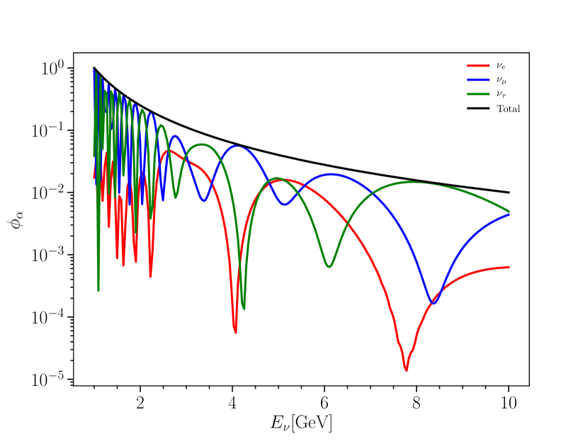
Figure 11: Result of propagating a power-law flux with spectral index of -1 through the Earth considering only oscillations and no interactions.

⬇

1interactions = True

2

3E_min = 1.0e2*units.GeV

4E_max = 1.0e8*units.GeV

5E_nodes = 200

6energy_nodes = nsq.logspace(E_min,E_max,E_nodes)

7

8neutrino_flavors = 3

9

10=======

11

12nuSQuIDS inputs should be given in natural units.

13In order to make this convenient, as in the {\ttf C++} code, we make use of the {\ttf SQuIDS} class {\ttf Const}.

14We can instantiate it as follows

15\begin{lstlisting}[language=Python, breaklines=true]

16units = nsq.Const()

As in the C++ $\nu$-SQuIDS interface one can propagate the neutrinos in various environments (see A.4 for further details). We can start by considering oscillactions in vacuum by setting:

⬇

nuSQ.Set_Body(nsq.Vacuum())

Since we have to specify that we are considering vacuum propagation, we must construct a trajectory inside that object. This can be done using the Track class-property of a given Body. Each Body will have its own Track subclass and its constructors. We can set and construct a vacuum trajectory in the following way:

⬇

nuSQ.Set_Track(nsq.Vacuum.Track(100.0*units.km))

Next we have to set the neutrino energy, which can be done as follows

⬇

nuSQ.Set_E(1.0*units.GeV)

Now we have to set the initial neutrino state. We can provide this state in either the flavor or mass basis. We can do this using the Set_initial_state function, providing it with a numpy array and a nsq.Basis. If the basis is nsq.Basis.flavor then the list must contain np.array([$\phi_{e}$,$\phi_{\mu}$,$\phi_{\tau}$]), similarly if enumeration is nsq.Basis.mass the list must specify $\phi_{i}$. In this example we set the initial state to $\nu_{\mu}$,

⬇

nuSQ.Set_initial_state(np.array([0.,1.,0.]),nsq.Basis.flavor)

Finally, we calculate the system evolution by

⬇

nuSQ.EvolveState()

After this runs, nuSQuIDS has evolved the state and holds it in memory. We can inquire for the flavor composition at this stage by

⬇

print([nuSQ.EvalFlavor(i) for i in range(3)])

which results in

⬇

[0.004675502573140013, 0.9022064087866011, 0.09311808864025879]

$\nu$-SQuIDS knows everything about the neutrino state at the current moment, it also knows what we did with it so far, where it went, what mixing parameters were used, etc. It would be convenient to store this information. One way of doing this is to serialize the $\nu$-SQuIDS status. We can do this in the following way

⬇

nuSQ.WriteStateHDF5("current_state.hdf5")

Everything that is in the $\nu$-SQuIDS object is now in that file. We can use that file to create a new $\nu$-SQuIDS object and do another calculation, we can stop the calculation midway and use it to restart, we can explore that file with other analysis tools, etc. In particular, the ‘ReadStateHDF5‘ will return us to the given configuration.

⬇

nuSQ.ReadStateHDF5("current_state.hdf5")

We can use the current tool to try to calculate $P(\nu_{\mu}\to\nu_{e})$ as a function of energy. We can do the following

⬇

1energy_values = np.linspace(1,10,40)

2nu_mu_to_nu_e = []

3for Enu in energy_values:

4 nuSQ.Set_E(Enu*units.GeV)

5 nuSQ.Set_initial_state(np.array([0.,1.,0.]),nsq.Basis.flavor)

6 nuSQ.EvolveState()

7 nu_mu_to_nu_e.append(nuSQ.EvalFlavor(0))

8

9plt.figure(figsize = (8,6))

10plt.xlabel(r"$E_\nu␣[{\rm␣GeV}]$")

11plt.ylabel(r"$P(\nu_\mu␣\to␣\nu_e)$")

12plt.plot(energy_values,nu_mu_to_nu_e, lw = 2, color = ’blue’)

This results in the plot shown in Figure 12 left panel.

Figure 12: Muon-neutrino to electron neutrino oscillation probability in vacuum as a function of the neutrino energy for a baseline of 100 km. The left panel is for the default standard oscillation parameters and the right panel has $\Delta m^{2}_{21}$ set to $1~{}{\rm eV}^{2}$

nuSQuIDs has some predefined oscillation mixing angles ($\theta_{ij}$) and mass splittings ($\Delta m^{2}_{ij}$), which we have taken from [22, 172]. We can change the square mass differences by using the following function

⬇

nuSQ.Set_SquareMassDifference(1,2.0e-1) # sets dm^2_{21} in eV^2.

Running the same script again results in the plot shown in Fig. 12 right panel.

We can also try to modify the mixing angles, for example

⬇

nuSQ.Set_MixingAngle(0,1,1.2) # sets \theta_{12} in radians.

nuSQ.Set_MixingAngle(0,2,0.3) # sets \theta_{23}} in radians.

nuSQ.Set_MixingAngle(1,2,0.4) # sets \theta_{23}} in radians.

We can also restore the default mixing angles and mass differences to default by doing

⬇

nuSQ.Set_MixingParametersToDefault()

C.3.3 Multiple-energy mode

In this section we will demonstrate the use of nuSQuIDS in the multiple energy mode. To begin we have to specify the $\{E_{i}\}$ grid where the equation will be solved. The energy nodes can be an arbitrary ordered list of energy in eV. The most common choice is to have linearly-spaced nodes or logarithmically-spaced nodes. For constructing numpy array of linear and logarithmic scales nuSQuIDS provides two convenient functions called linspace and logspace respectively. The following lines define the energy grid and construct the nuSQUIDS object.

⬇

1interactions = False

2

3E_min = 1.0*units.GeV

4E_max = 10.0*units.GeV

5E_nodes = 101

6

7energy_nodes = nsq.logspace(E_min,E_max,E_nodes)

8

9neutrino_flavors = 3

10

11nuSQ = nsq.nuSQUIDS(energy_nodes,neutrino_flavors,nsq.NeutrinoType.neutrino,interactions)

We can propagate a neutrino ensemble through the Earth in an atmospheric neutrino telescope setting. We can do that by setting the following Body and Track:

⬇

1earth = nsq.EarthAtm()

2nuSQ.Set_Body(earth)

3nuSQ.Set_Track(earth.MakeTrackWithCosine(-1))

For the initial flux we will assume that it’s given by $\phi_{\nu}=N_{0}E^{-2}$, with flavor composition $\phi_{e}:\phi_{\mu}:\phi_{\tau}$ = $0:1:0$. $\nu$-SQuIDS input flux is a numpy.ndarray formatted in the following way:

$$InputState\doteq[[\phi^{1}_{e},\phi^{1}_{\mu},\phi^{1}_{\tau}],...,[\phi^{i}_{e},\phi^{i}_{\mu},\phi^{i}_{\tau}],...,[\phi^{n}_{e},\phi^{n}_{\mu},\phi^{n}_{\tau}]]$$ (22)

where $i=1$ to $n$ and $n$ is the number of energy nodes. We can implement this in the following way

⬇

1N0 = 1.0e18

2Eflux = lambda E: N0*E**-2

3Einitial = (Eflux(nuSQ.GetERange()).reshape((101,1)))*(np.array([0.,1.,0.]).reshape(1,3))

where N0 is an arbitrary normalization constant, but we have chosen it such that the input flux is $O(1)$.

⬇

1nuSQ.Set_initial_state(Einitial,nsq.Basis.flavor)

2

3nuSQ.Set_rel_error(1.0e-17)

4nuSQ.Set_abs_error(1.0e-17)

5

6nuSQ.EvolveState()

Then we can evaluate the resulting flux and plot the resulting oscillation probabilities by using the folowing script

⬇

1e_range = np.linspace(1.0,10.0,200)

2

3nu_e = np.array([nuSQ.EvalFlavor(0,EE*units.GeV,0)

4 for EE in e_range])

5nu_mu = np.array([nuSQ.EvalFlavor(1,EE*units.GeV,0)

6 for EE in e_range])

7nu_tau = np.array([nuSQ.EvalFlavor(2,EE*units.GeV,0)

8 for EE in e_range])

9

10total = nu_e + nu_mu + nu_tau

11

12plt.figure(figsize = (8,6))

13

14plt.xlabel(r"$E_\nu␣[{\rm␣GeV}]$")

15plt.ylabel(r"$\phi_\alpha$")

16

17plt.plot(e_range,nu_e, lw = 2, color = ’red’, label = r"$\nu_e$")

18plt.plot(e_range,nu_mu, lw = 2, color = ’blue’, label = r"$\nu_\mu$")

19plt.plot(e_range,nu_tau, lw = 2, color = ’green’, label = r"$\nu_\tau$")

20plt.plot(e_range,total, lw = 2, color = ’black’, label = r"Total")

21plt.legend(fancybox = True, fontsize = 10)

22plt.semilogy()

The result of this is shown in the left panel of Fig. 13. Our final example is performing the full nuSQuIDS calculation with neutrinos and antineutrinos, but this time including interactions

Figure 13: Result of propagating a power-law flux with spectral index of -1 through the Earth considering only oscillations and no interactions.

⬇

1interactions = True

2

3E_min = 1.0e2*units.GeV

4E_max = 1.0e8*units.GeV

5E_nodes = 200

6energy_nodes = nsq.logspace(E_min,E_max,E_nodes)

7

8neutrino_flavors = 3

9

10>>>>>>> c6a8be92b35067939fa5267703c6d8ea03949c30

11nuSQ = nsq.nuSQUIDS(energy_nodes,neutrino_flavors,nsq.NeutrinoType.both,interactions)

In this case we need to specify the neutrino and antineutrino initial fluxes. Those have the following format:

$$InputState\doteq[[[\phi^{1}_{e},\phi^{1}_{\mu},\phi^{1}_{\tau}],[\bar{\phi}^{1}_{e},\bar{\phi}^{1}_{\mu},\bar{\phi}^{1}_{\tau}]],...,[[\phi^{i}_{e},\phi^{i}_{\mu},\phi^{i}_{\tau}],[\bar{\phi}^{i}_{e},\bar{\phi}^{i}_{\mu},\bar{\phi}^{i}_{\tau}]],...,[[\phi^{n}_{e},\phi^{n}_{\mu},\phi^{n}_{\tau}],[\bar{\phi}^{n}_{e},\bar{\phi}^{n}_{\mu},\bar{\phi}^{n}_{\tau}]]]$$

where $i=1$ to $n$ and $n$ is the number of energy nodes and $\phi$ ($\bar{\phi}$) is the neutrino (antineutrino) flux. We can implement this as follows

⬇

1N0 = 1.0e18; Power = -1.0

2Eflux = lambda E: N0*E**Power

3

4InitialFlux = np.zeros((200,2,3))

5for i,E in enumerate(nuSQ.GetERange()):

6 InitialFlux[i][0][0] = 0.0

7 InitialFlux[i][1][0] = 0.0

8 InitialFlux[i][0][1] = Eflux(E)

9 InitialFlux[i][1][1] = Eflux(E)

10 InitialFlux[i][0][2] = Eflux(E)

11 InitialFlux[i][1][2] = Eflux(E)

⬇

1nuSQ.Set_MixingParametersToDefault()

2earth = nsq.EarthAtm()

3nuSQ.Set_Body(earth)

4nuSQ.Set_Track(earth.MakeTrackWithCosine(-1))

5nuSQ.Set_initial_state(InitialFlux,nsq.Basis.flavor)

An important phenomena in this scenario is that of tau-regeneration, which we can enable by

⬇

nuSQ.Set_TauRegeneration(True)

After doing the evolution we can evaluate the resulting flux by doing:

⬇

1nu_tau = np.array([ nuSQ.EvalFlavorAtNode(2,ie,0) for ie,EE in enumerate(nuSQ.GetERange())])

2nu_tau_bar = np.array([ nuSQ.EvalFlavorAtNode(2,ie,1) for ie,EE in enumerate(nuSQ.GetERange())])

3

4nu_mu = np.array([ nuSQ.EvalFlavorAtNode(1,ie,0) for ie,EE in enumerate(nuSQ.GetERange())])

5nu_mu_bar = np.array([ nuSQ.EvalFlavorAtNode(1,ie,1) for ie,EE in enumerate(nuSQ.GetERange())])

and plot it by using this script

⬇

1plt.figure(figsize = (6,6))

2plt.xlabel(r"$E_\nu␣[{\rm␣GeV}]$")

3plt.ylabel(r"${\rm␣E_\nu}␣\times␣\phi_\nu␣(E_\nu)$")

4e_range = nuSQ.GetERange()/units.GeV

5plt.plot(e_range,0.5*(nu_tau+nu_tau_bar)*(e_range*units.GeV)/N0, lw = 3, label =r"$\nu_\tau␣+␣\bar{\nu}_\tau$", color = "blue")

6plt.plot(e_range,0.5*(nu_mu+nu_mu_bar)*(e_range*units.GeV)/N0, lw = 3, label =r"$\nu_\mu␣+␣\bar{\nu}_\mu$", color = "red")

7plt.axhline (1.0, color = "k", lw = 3)

8plt.xlim(1.0e2,1.0e6)

9plt.ylim(1.0e-2,1.0e1)

10plt.grid()

11plt.loglog()

12plt.legend(loc = "upper␣right", fancybox = True, fontsize = 15)

The result of this is shown in Fig. 14.

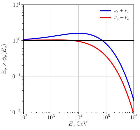
Figure 14: Propagated flux for muon and tau neutrinos through the Earth including the effect of tau regeneration.

C.4 SU_vector operations in Python 

SQuIDS SU_vector class provides a combinent way to perform operations that commonly arise in quantum mechanics. For this reason we have also make them available in the Python interface. All of the SU_vector operations have been implemented, but due to optimizations performed in the C++ some notes are in order.

We can compute the SU_vector that represents a typical neutrino Hamiltonian in three flavors as

⬇

1import nuSQUIDSpy as nsq

2p2=nsq.SU_vector.Projector(3,1)

3dm12=1e-5

4H=p2*dm12

In this code snippet p2 is a SU_vector, but H is a SU_vector::MultiplicationProxy. In the C++ implementation these proxies appear when operations are performed on SU_vector objects to optimize memory usage, as described earlier in this document. To keep operating on these objects one needs to cast them onto real SU_vector rather than proxies for them. This can be done as follows:

⬇

1H=nsq.SU_vector(H)

after which H is a real vector and can be operated upon. This same conversion needs to be performed explicitly every time a proxy is encountered in Python.

C.5 Extending the interface with user-defined classes 

In this section we briefly show how to construct python bindings for user-defined classes. As an example we have an extension class called nuSQUIDSExt defined as:

⬇

1class nuSQUIDSExt : public nuSQUIDS {

2 ...

3 public:

4 nuSQUIDSExt(); // default constructor

5 nuSQUIDSExt(double x); // constructor

6 double FunctionExtension(double x); // function of interest

7 ...

8}

where this class has two constructors and one function of interest which we would like to expose to Python. In order to construct the python module we need to make a new C++ source file with the following content.

⬇

1#include "nuSQUIDSpy.h"

2#include "nuSQUIDSExt.h"

3

4BOOST_PYTHON_MODULE(nuSQUIDSExtensionPythonModuleName)

5{

6 // Register all standard nuSQuIDS and nuSQuIDS atmospheric functions for the user class

7 auto nusquidsext_register = RegisterBasicNuSQuIDSPythonBindings<nuSQUIDSExt>("nuSQUIDSExt");

8 auto nusquidsext_atm_register = RegisterBasicAtmNuSQuIDSPythonBindings<nuSQUIDSExt>("nuSQUIDSExtAtm");

9 // Register additional functions or members of the user class

10 auto nusquidsext_class_object = nusquidsext_register.GetClassObject();

11 nusquidsext_class_object->def("FuctionExtension",&nuSQUIDSExt::FunctionExtension);

12}

where the header nuSQUIDSpy.h contains the nuSQUIDS python binding utilities and definitions, and nuSQUIDSExt.h is the header where the new class of interest is defined. In this code we have used two template structures, whose constructors are:

• ⬇

  RegisterBasicNuSQuIDSPythonBindings<nuSQUIDSDerivedType>(std::string name);

  The type of the extension has to be a nuSQUIDS derived type, in this case
  nuSQUIDSDerivedType is nuSQUIDSExt. The string that is passed as an argument does not need to match the type name and is how the class will be named in Python. This class will register all the functions that it inherits as a nuSQUIDS derived class, but not any new members introduced by the user.

• ⬇

  RegisterBasicAtmNuSQuIDSPythonBindings<nuSQUIDSDerivedType>(std::string name);

  The type of the extension has to be a nuSQUIDS derived type, in this case
  nuSQUIDSDerivedType is nuSQUIDSExt. The string that is passed as an argument does not need to match the type name and is how the class will be named in Python. This class will register all the functions that it inherits as a nuSQUIDSAtm<Type> derived class, but not any new members introduced by the user.

This module needs to be compiled with the same dependencies as our nominal python bindings, for which we suggest the user to copy our Makefile and modify the name of the library to be generated to match the module name. As a final step the user should place the resulting shared object library in the system PYTHONPATH.

Appendix D Singly-Differential Cross-Section Tabulation

Efforts to precisely and consistently capture the physics of the singly-differential DIS cross sections have lead to using a slightly unusual tabulation scheme, the details of which we describe here.

First, in order to interpolate cross section values for arbitrary incident and out-going energies, it is convenient that values be tabulated on some rectangular grid. The natural choice is to use a common set of out-going energies energies for all incident energies. Clearly, such a set of out-going energies should extend up to the maximum tabulated incident energy. However, the cross section is meaningless for out-going energies greater than the incident energy, so for all table rows corresponding to incident energies less than the maximum tabulated, some of the higher out-going energy entries will be undefined, and must be filled with some dummy value (or a non-rectangular storage format must be used). This layout is shown in the left panel of Fig. 15. The presence of this diagonal boundary through the table between physical and unphysical regions frustrates simple interpolation schemes in the region near the boundary, as the method used must not allow the undefined or placeholder values to contribute to the calculation of the interpolated value. This can be addressed by switching interpolation methods depending on location in the table (such as using linear interpolation via barycentric coordinates on a triangle for points in cells with only three physically allowed corner points but typical rectangular bilinear interpolation in other cells), but this adds complexity and is hostile to using higher-order interpolation methods. As a more minor point, when typical rectangular storage formats are used, the unphysical region wastes storage space.

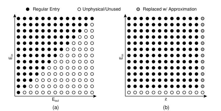
Figure 15: Schematic depiction of the two tabulation schemes discussed for singly-differential cross sections. (a) shows simple tabulation in $E_{in}$ and $E_{out}$, while (b) shows the scheme introduced here using $E_{in}$ and the transformed $z$ variable, and indicates the $z=1$ entries which are replaced by the values chosen to approximate the peak as a function of $E_{out}$ or $z$. It is assumed that $E_{out}$ ranges over the same set of values as $E_{in}$, and that $z$ ranges over [0, 1].

Second, the cross sections have considerable curvature, which leads to systematic errors when linear interpolation is used. These errors are illustrated in the lower panel of Fig. 16 where the relative error of the interpolated cross section grows periodically to between the tabulated cross section points. It should be the case that the integral of the singly-differential cross section over out-going energy for a given incident energy should equal the total cross section (up to truncation effects due to the limited domain of tabulation). If this is not the case, errors gradually accumulate when solving the evolution of a neutrino flux undergoing interactions with matter, producing non-physical artifacts in the final computed flux. This effect is particularly pernicious because it is difficult to detect in calculations using a coarse energy node spacing, with its nature only becoming clearly evident for node spacings finer than the cross section tabulation spacing. Importantly, neither calculation will be correct, but efforts to determine a suitably dense node spacing can be frustrated by the appearance of the unphysical artifacts when more dense spacing are tested for comparison.

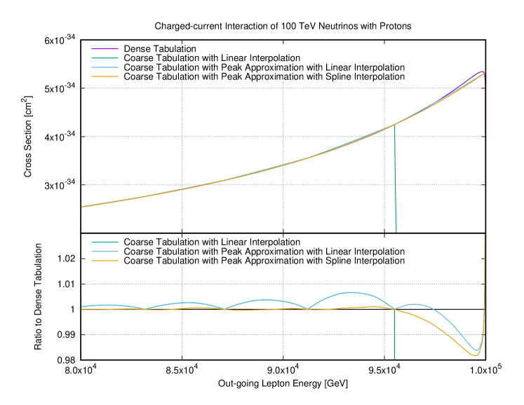
Figure 16: Illustration of problems interpolating the singly-differential DIS cross section at high energies and the effects of different mitigations discussed in the text. The ‘Dense Tabulation’ represents an essentially ideal treatment which unfortunately uses far too many samples for general practicality (10,000 samples per decade in $E_{out}$). The ‘Coarse Tabulation’ uses are more normal 50 samples per decade. The tabulation points for the coarse table are visible as the points in the the lower panel where the error of the interpolation disappears, since the values tabulated in both tables are identical where they both exist. The linear interpolation of the coarse table is efficient to compute, but has problematically large errors in near the centers of the table bins due to being unable to represent curvature. Approximation with cubic splines greatly reduces this type of error. Simple interpolation with the final table entry (for $E_{out}=E_{in}$) being the formally correct zero value shows a very large error due to entirely missing the peak of the function. Replacing the final sample with a carefully chosen approximation eliminates this severe effect, although the true shape of the peak still cannot be captured.

Third, as incident neutrino energies increase, the cross section as a function of out-going energy develops a sharp peak structure for out-going energies close to the incident energy. Inevitably this peak will at some energy become too narrow to be sampled accurately by the tabulation spacing, whatever it has been chosen to be. This problem is greatly exacerbated by the additional fact that when the out-going energy is equal to the incident energy, the cross section must be zero. Taken literally, this forces the final table entry in each row to be zero, which causes the interpolation between the last two table entries to fall sharply, even when one would wish for it to first rise to the peak. Since a large portion of the integral of the differential cross section can be contained in this peak this causes a sizable discrepancy between the integral of the (interpolated) differential cross section and the total cross section. This is illustrated in Fig. 16 by the severe disagreement between the ideal sufficiently dense tabulation and the (practically realizable) coarse tabulation with linear interpolation over the latter’s last table bin.

To address the first and second problems, it is desirable to use a rectangular tabulation which has no unphysical entries and will permit simple use of higher order interpolation methods, such as cubic splines (or bicubic interpolation based on cubic splines, given the two-dimensional nature of the table). It is therefore useful to introduce a variable $z$:

$$z={E_{out}-E_{out,min}\over E_{in}-E_{out,min}}$$ (23)

where $E_{in}$ is the incident neutrino energy, $E_{out}$ is the out-going lepton energy, and $E_{out,min}$ is the minimum tabulated out-going lepton energy. This variable has the property that for $E_{out}$ ranging over $[E_{out,min},E_{in}]$, $z$ takes on values from $[0,1]$ for all $E_{in}$. If one tabulates in some set of $z$ values distributed over $[0,1]$, the range of $E_{out}$ values covered will differ for different $E_{in}$, but in a useful way, since all will be physically meaningful, and while no $E_{out}$ values except $E_{out,min}$ will generally be shared between different $E_{in}$ values, this does no particular harm, since interpolation can simply be performed in the $(E_{in},z)$ space. Tabulation in $z$ eliminates the first concern and significantly mitigates the second by enabling convenient use of higher order interpolation schemes, as shown in Fig. 16, where the spline interpolation shows greatly reduced errors for all except the last bin (which merits a separate discussion) compared to the linear interpolation. It should be noted that $z$ is undefined for $E_{in}=E_{out,min}$, but there can be no non-zero cross section for this table row (shown in the right panel Fig. 15 as white points) if it is included anyway, so nuSQuIDS will never explicitly refer to these entries and they can be safely set to any convenient values (such as values similar to the entries for the next row with greater $E_{out}$, in order to give well-behaved interpolation).

Unfortunately, tabulation in $z$ does nothing useful to address the third concern. More additional, valid tabulated values are added for lower incident energies, which have less need to resolve a sharp peak. Instead, another approach is needed. As previously mentioned, the $E_{out}=E_{in}$ (or $z=1$) column of the table (shown as gray points in the right panel of Fig. 15) is known to always be formally zero, and so like the $E_{in}=E_{out,min}$ row it is not explicitly needed. Since this column is also a major driver of the bad interpolation of the peak when it is unresolvable inside the final table bin, replacing it is doubly useful for changing the interpolation to be something more suitable. Since the only strictly physically correct value to place in this column is zero, any other choice is an approximation, and which approximation is ‘best’ is a matter of interpretation. Since the shape of the peak itself cannot be represented faithfully, we choose to attempt to preserve its integral instead, and choose to replace the final entry in the row with one selected so that the average of the last two values is equal to the true average computed from a detailed integral of the cross section over the bin. That is, if $T_{i}$ are the tabulated cross section values, of which there are $N$ in the table row, we set:

$$T_{N}={2\over y(E_{out,N})-y(E_{out,N-1})}\int^{y(E_{out,N})}_{y(E_{out,N-1})}{{d\sigma\over dy}dy}-T_{N-1}$$ (24)

where $y$ is the standard scaling variable $y=(E_{in}-E_{out})/E_{in}$. This choice gives the correct integral when the table is interpolated linearly, and gives similarly close results for common choices of higher-order interpolation, and can be interpreted as ‘smearing out’ the contribution of the peak uniformly across the table bin in a cumulative sense. The two curves shown in Fig. 16 with ‘Peak Approximation’ in their labels show this scheme in action. While some residual error in the interpolated cross section remains due to the approximation cutting through the peak rather than following it exactly, the situation is vastly improved over the interpolation without approximation which drops rapidly to zero (extremely so, due to interpolation being done in the space of the logarithm of the cross section). From the figure it is clear that this much more accurately captures the contribution of this bin to the integral.

Appendix E Test suite

A test suite is provided with the library to guarantee the right output in different systems or after any modification of the code. All the tests are located in the folder nuSQuIDS/test And they can be run using the provided script test/run_tests. A single test can be run by adding the name as an argument to the script command. In the following we list the tests that are provided with a brief description of what they test.

• test/vacuum_osc_prob.test

  Tests that propagation with only oscillation of neutrinos in vacuum is equal to the analytic solution.

• test/constant_density_osc_prob.test

  Tests that propagation with only oscillation of neutrinos in constant density is equal to the analytic solution.

• test/constant_opacity.test

  Tests that propagation on a constant density with no oscillation and neglecting regeneration from neutral current or tau decay matches the expected exponential behavior.

• test/constant_opacity_with_nc.test

  Tests that propagation on a constant density with no oscillation matches an independent numerical solution.

• test/atmospheric_he.test

  Tests that the high-energy propagation without oscillation of neutrinos from the atmosphere does not give negative or nan values.

• test/atmospheric_osc.test

  Tests that propagation with only oscillation of neutrinos from the atmosphere does not give negative or nan values.

• test/body_serialization.test

  It checks that writing a body in to the hdf5 file and reading it back does not alter the body.

• test/cross_section_consistency.test

  Checks that the differential cross section adds, within numerical error, to the total cross section.

• test/earth_osc_prob.test

  Test that three and four neutrinos oscillation probability over a 1000km baseline in multiple and single energy modes matches with the numerical error to a reference independent calculation.

• test/glashow_resonance.test

  Checks that Glashow resonance integrated differential cross-section matches with the total cross-section and that is used while propagating.

• test/hdf5_atm_in_out.test

  It checks that writing a nuSQuIDs atmospheric object into a hdf5 file and reading it back does not alter the object and recovers all the properties.

• test/hdf5_in_out.test

  It checks that writing a nuSQuIDs object into a hdf5 file and reading it back does not alter the object and recovers all the properties.

• test/move_assig.test

  Checks that constructor of a nuSQuIDS object from an rvalue nuSQuIDS object works.

• test/mul_energy_constructor.test

  Checks that the multiple energy constructor works.

• test/time_reversal.test

  Checks that propagating a neutrino and propagating again backwards in time returns to the original state.

• test/tools_integrator.test

  Checks that the provided one dimensional integrate function works within the numerical error.

• test/track_concatenate_hdf5.test

  Checks that propagating by concatenating a series of tracks in vacuum and writing and reading that state at every step is the same as propagating with a single track with the total length.

• test/track_concatenate.test

  Checks that propagating by concatenating a series of tracks in vacuum is the same as propagating with a single track with the total length.

• test/external_flux.test

  Checks that the emitting body feature works. This is done by propagating an initially empty neutrino ensemble on a medium that emits neutrinos and comparing the result with an analytical solution.

References

- [1] K. Abe, et al., Solar neutrino results in Super-Kamiokande-III, Phys. Rev. D 83 (2011) 052010. arXiv:1010.0118, doi:10.1103/PhysRevD.83.052010.
- [2] G. Bellini, et al., Final results of Borexino Phase-I on low energy solar neutrino spectroscopy, Phys. Rev. D 89 (11) (2014) 112007. arXiv:1308.0443, doi:10.1103/PhysRevD.89.112007.
-
[3]
M. G. e. a. Aartsen,
Determining
neutrino oscillation parameters from atmospheric muon neutrino disappearance
with three years of icecube deepcore data, Phys. Rev. D 91 (2015) 072004.
doi:10.1103/PhysRevD.91.072004.
URL http://link.aps.org/doi/10.1103/PhysRevD.91.072004 - [4] E. Richard, et al., Measurements of the atmospheric neutrino flux by Super-Kamiokande: energy spectra, geomagnetic effects, and solar modulation, Phys. Rev. D 94 (5) (2016) 052001. arXiv:1510.08127, doi:10.1103/PhysRevD.94.052001.
- [5] M. G. Aartsen, et al., Measurement of Atmospheric Tau Neutrino Appearance with IceCube DeepCore, Phys. Rev. D 99 (3) (2019) 032007. arXiv:1901.05366, doi:10.1103/PhysRevD.99.032007.
- [6] A. Albert, et al., Measuring the atmospheric neutrino oscillation parameters and constraining the 3+1 neutrino model with ten years of ANTARES data, JHEP 06 (2019) 113. arXiv:1812.08650, doi:10.1007/JHEP06(2019)113.
-
[7]
K. e. a. Abe,
Precise
measurement of the neutrino mixing parameter
from muon neutrino disappearance in an off-axis beam, Phys. Rev. Lett. 112
(2014) 181801.
doi:10.1103/PhysRevLett.112.181801.
URL http://link.aps.org/doi/10.1103/PhysRevLett.112.181801 -
[8]
P. e. a. Adamson,
First measurement
of muon-neutrino disappearance in nova, Phys. Rev. D 93 (2016) 051104.
doi:10.1103/PhysRevD.93.051104.
URL http://link.aps.org/doi/10.1103/PhysRevD.93.051104 -
[9]
P. e. a. Adamson,
First
measurement of electron neutrino appearance in nova, Phys. Rev. Lett. 116
(2016) 151806.
doi:10.1103/PhysRevLett.116.151806.
URL http://link.aps.org/doi/10.1103/PhysRevLett.116.151806 -
[10]
P. e. a. Adamson,
Measurement of
neutrino and antineutrino oscillations using beam and atmospheric data in
minos, Phys. Rev. Lett. 110 (2013) 251801.
doi:10.1103/PhysRevLett.110.251801.
URL http://link.aps.org/doi/10.1103/PhysRevLett.110.251801 - [11] F. P. An, et al., Spectral measurement of electron antineutrino oscillation amplitude and frequency at Daya Bay, Phys. Rev. Lett. 112 (2014) 061801. arXiv:1310.6732, doi:10.1103/PhysRevLett.112.061801.
- [12] Y. Abe, et al., Measurement of in Double Chooz using neutron captures on hydrogen with novel background rejection techniques, JHEP 01 (2016) 163. arXiv:1510.08937, doi:10.1007/JHEP01(2016)163.
- [13] S.-B. Kim, Measurement of neutrino mixing angle and mass difference from reactor antineutrino disappearance in the RENO experiment, Nucl. Phys. B908 (2016) 94–115. doi:10.1016/j.nuclphysb.2016.02.036.
- [14] B. Pontecorvo, Neutrino Experiments and the Problem of Conservation of Leptonic Charge, Sov.Phys.JETP 26 (1968) 984–988.
- [15] V. Gribov, B. Pontecorvo, Neutrino astronomy and lepton charge, Phys.Lett. B28 (1969) 493. doi:10.1016/0370-2693(69)90525-5.
-
[16]
M. Fukugita, T. Yanagida,
Physics of Neutrinos: And
Applications to Astrophysics, Physics and astronomy online library,
Springer, 2003.
URL http://books.google.fr/books?id=El8R8nC5QegC - [17] E. K. Akhmedov, Neutrino physics (1999) 103–164arXiv:hep-ph/0001264.
-
[18]
A. B. Balantekin, W. C. Haxton, Neutrino
oscillationsarXiv:1303.2272.
URL http://arxiv.org/abs/1303.2272 - [19] M. Gonzalez-Garcia, M. Maltoni, Phenomenology with Massive Neutrinos, Phys.Rept. 460 (2008) 1–129. arXiv:0704.1800, doi:10.1016/j.physrep.2007.12.004.
-
[20]
R. M. et al., Theory of neutrinos: A
white paperarXiv:hep-ph/0510213.
URL http://arxiv.org/abs/hep-ph/0510213 -
[21]
A. de Gouvea et al., NeutrinosarXiv:1310.4340.
URL http://arxiv.org/abs/1310.4340 - [22] I. Esteban, M. Gonzalez-Garcia, M. Maltoni, T. Schwetz, A. Zhou, The fate of hints: updated global analysis of three-flavor neutrino oscillations, JHEP 09 (2020) 178. arXiv:2007.14792, doi:10.1007/JHEP09(2020)178.
- [23] P. F. de Salas, D. V. Forero, C. A. Ternes, M. Tortola, J. W. F. Valle, Status of neutrino oscillations 2018: 3 hint for normal mass ordering and improved CP sensitivity, Phys. Lett. B782 (2018) 633–640. arXiv:1708.01186, doi:10.1016/j.physletb.2018.06.019.
- [24] F. Capozzi, E. Lisi, A. Marrone, A. Palazzo, Current unknowns in the three neutrino framework, Prog. Part. Nucl. Phys. 102 (2018) 48–72. arXiv:1804.09678, doi:10.1016/j.ppnp.2018.05.005.
- [25] P. F. de Salas, D. V. Forero, S. Gariazzo, P. Martínez-Miravé, O. Mena, C. A. Ternes, M. Tórtola, J. W. F. Valle, 2020 global reassessment of the neutrino oscillation picture, JHEP 02 (2021) 071. arXiv:2006.11237, doi:10.1007/JHEP02(2021)071.
-
[26]
J. H. et al., Fundamental physics at the
intensity frontierarXiv:1205.2671.
URL http://arxiv.org/abs/1205.2671 - [27] R. Acciarri, et al., Long-Baseline Neutrino Facility (LBNF) and Deep Underground Neutrino Experiment (DUNE)arXiv:1601.05471.
- [28] M. G. Aartsen, et al., Letter of Intent: The Precision IceCube Next Generation Upgrade (PINGU)arXiv:1401.2046.
- [29] A. Kouchner, KM3NeT - ORCA: measuring the neutrino mass ordering in the Mediterranean, J. Phys. Conf. Ser. 718 (6) (2016) 062030. doi:10.1088/1742-6596/718/6/062030.
- [30] G. De Rosa, Status and neutrino oscillation physics potential of the Hyper-Kamiokande Project in Japan, J. Phys. Conf. Ser. 718 (6) (2016) 062014. doi:10.1088/1742-6596/718/6/062014.
- [31] A. Donini, S. Palomares-Ruiz, J. Salvado, Neutrino tomography of the EartharXiv:1803.05901.
- [32] M. Bustamante, A. Connolly, Extracting the Energy-Dependent Neutrino-Nucleon Cross Section above 10 TeV Using IceCube Showers, Phys. Rev. Lett. 122 (4) (2019) 041101. arXiv:1711.11043, doi:10.1103/PhysRevLett.122.041101.
- [33] R. Abbasi, et al., Measurement of the high-energy all-flavor neutrino-nucleon cross section with IceCubearXiv:2011.03560, doi:10.1103/PhysRevD.104.022001.
- [34] M. G. Aartsen, et al., Observation of High-Energy Astrophysical Neutrinos in Three Years of IceCube Data, Phys. Rev. Lett. 113 (2014) 101101. arXiv:1405.5303, doi:10.1103/PhysRevLett.113.101101.
- [35] M. G. Aartsen, et al., Searches for Sterile Neutrinos with the IceCube DetectorarXiv:1605.01990.
- [36] M. G. Aartsen, et al., Evidence for Astrophysical Muon Neutrinos from the Northern Sky with IceCube, Phys. Rev. Lett. 115 (8) (2015) 081102. arXiv:1507.04005, doi:10.1103/PhysRevLett.115.081102.
- [37] R. Abbasi, et al., The IceCube high-energy starting event sample: Description and flux characterization with 7.5 years of data, Phys. Rev. D 104 (2021) 022002. arXiv:2011.03545, doi:10.1103/PhysRevD.104.022002.
- [38] C. A. Argüelles, T. Katori, J. Salvado, New Physics in Astrophysical Neutrino Flavor, Phys. Rev. Lett. 115 (2015) 161303. arXiv:1506.02043, doi:10.1103/PhysRevLett.115.161303.
- [39] M. Bustamante, J. F. Beacom, W. Winter, Theoretically palatable flavor combinations of astrophysical neutrinos, Phys. Rev. Lett. 115 (16) (2015) 161302. arXiv:1506.02645, doi:10.1103/PhysRevLett.115.161302.
- [40] P. Baerwald, M. Bustamante, W. Winter, Neutrino Decays over Cosmological Distances and the Implications for Neutrino Telescopes, JCAP 1210 (2012) 020. arXiv:1208.4600, doi:10.1088/1475-7516/2012/10/020.
- [41] C. A. Arguelles, M. Bustamante, A. Kheirandish, S. Palomares-Ruiz, J. Salvado, A. C. Vincent, Fundamental physics with high-energy cosmic neutrinos today and in the future, PoS ICRC2019 (2020) 849, 36th International Cosmic Ray Conference (ICRC 2019), Madison, WI, U.S.A. arXiv:1907.08690.
- [42] I. Esteban, S. Pandey, V. Brdar, J. F. Beacom, Probing Secret Interactions of Astrophysical Neutrinos in the High-Statistics EraarXiv:2107.13568.
- [43] R. Davis, Jr., D. S. Harmer, K. C. Hoffman, Search for neutrinos from the sun, Phys. Rev. Lett. 20 (1968) 1205–1209. doi:10.1103/PhysRevLett.20.1205.
- [44] H. A. Bethe, A Possible Explanation of the Solar Neutrino Puzzle, Phys. Rev. Lett. 56 (1986) 1305. doi:10.1103/PhysRevLett.56.1305.
- [45] V. D. Barger, R. J. N. Phillips, K. Whisnant, Solar neutrino solutions with matter enhanced flavor changing neutral current scattering, Phys. Rev. D44 (1991) 1629–1643. doi:10.1103/PhysRevD.44.1629.
- [46] E. Roulet, MSW effect with flavor changing neutrino interactions, Phys. Rev. D44 (1991) 935–938. doi:10.1103/PhysRevD.44.R935.
- [47] M. C. Gonzalez-Garcia, M. Maltoni, J. Salvado, Testing matter effects in propagation of atmospheric and long-baseline neutrinos, JHEP 05 (2011) 075. arXiv:1103.4365, doi:10.1007/JHEP05(2011)075.
- [48] M. C. Gonzalez-Garcia, M. Maltoni, Determination of matter potential from global analysis of neutrino oscillation data, JHEP 09 (2013) 152. arXiv:1307.3092, doi:10.1007/JHEP09(2013)152.
-
[49]
M. Pospelov, Neutrino physics with dark
matter experiments and the signature of new baryonic neutral currentsarXiv:1103.3261.
URL http://arxiv.org/abs/1103.3261 -
[50]
J. Kopp, J. Welter, The not-so-sterile
4th neutrino: Constraints on new gauge interactions from neutrino oscillation
experimentsarXiv:1408.0289.
URL http://arxiv.org/abs/1408.0289 - [51] M. Maltoni, A. Yu. Smirnov, Solar neutrinos and neutrino physics, Eur. Phys. J. A52 (4) (2016) 87. arXiv:1507.05287, doi:10.1140/epja/i2016-16087-0.
- [52] I. Esteban, M. C. Gonzalez-Garcia, M. Maltoni, I. Martinez-Soler, J. Salvado, Updated Constraints on Non-Standard Interactions from Global Analysis of Oscillation Data, JHEP 08 (2018) 180. arXiv:1805.04530, doi:10.1007/JHEP08(2018)180.
-
[53]
A. A. et al., Evidence for neutrino
oscillations from the observation of electron anti-neutrinos in a muon
anti-neutrino beamarXiv:hep-ex/0104049.
URL http://arxiv.org/abs/hep-ex/0104049 -
[54]
G. Mention, M. Fechner, T. Lasserre, T. A. Mueller, D. Lhuillier, M. Cribier,
A. Letourneau, The reactor antineutrino
anomalyarXiv:1101.2755.
URL http://arxiv.org/abs/1101.2755 -
[55]
MiniBooNE-Collaboration, A combined
and oscillation analysis of
the miniboone excessesarXiv:1207.4809.
URL http://arxiv.org/abs/1207.4809 - [56] A. A. Aguilar-Arevalo, et al., Observation of a Significant Excess of Electron-Like Events in the MiniBooNE Short-Baseline Neutrino ExperimentarXiv:1805.12028.
- [57] I. Alekseev, et al., DANSS: Detector of the reactor AntiNeutrino based on Solid Scintillator, JINST 11 (11) (2016) P11011. arXiv:1606.02896, doi:10.1088/1748-0221/11/11/P11011.
- [58] Y. Ko, et al., Sterile Neutrino Search at the NEOS Experiment, Phys. Rev. Lett. 118 (12) (2017) 121802. arXiv:1610.05134, doi:10.1103/PhysRevLett.118.121802.
- [59] J. Ashenfelter, et al., First search for short-baseline neutrino oscillations at HFIR with PROSPECTarXiv:1806.02784.
- [60] Y. Abreu, et al., Performance of a full scale prototype detector at the BR2 reactor for the SoLid experiment, JINST 13 (05) (2018) P05005. arXiv:1802.02884, doi:10.1088/1748-0221/13/05/P05005.
- [61] Dentler, Mona and Hernández-Cabezudo, Álvaro and Kopp, Joachim and Machado, Pedro A. N. and Maltoni, Michele and Martinez-Soler, Ivan and Schwetz, Thomas, Updated Global Analysis of Neutrino Oscillations in the Presence of eV-Scale Sterile Neutrinos, JHEP 08 (2018) 010. arXiv:1803.10661, doi:10.1007/JHEP08(2018)010.
- [62] J. Kopp, P. A. Machado, M. Maltoni, T. Schwetz, Sterile neutrino oscillations: the global picture, Journal of High Energy Physics 2013 (5) (2013) 1–52.
- [63] G. H. Collin, C. A. Argüelles, J. M. Conrad, M. H. Shaevitz, Sterile Neutrino Fits to Short Baseline Data, Nucl. Phys. B908 (2016) 354–365. arXiv:1602.00671, doi:10.1016/j.nuclphysb.2016.02.024.
-
[64]
K. N. A. et al., Light sterile neutrinos:
A white paperarXiv:1204.5379.
URL http://arxiv.org/abs/1204.5379 - [65] M. Blennow, E. Fernandez-Martinez, J. Gehrlein, J. Hernandez-Garcia, J. Salvado, IceCube bounds on sterile neutrinos above 10 eVarXiv:1803.02362.
- [66] A. Diaz, C. Argüelles, G. Collin, J. Conrad, M. Shaevitz, Where Are We With Light Sterile Neutrinos?arXiv:1906.00045.
- [67] S. Böser, C. Buck, C. Giunti, J. Lesgourgues, L. Ludhova, S. Mertens, A. Schukraft, M. Wurm, Status of Light Sterile Neutrino Searches, Prog. Part. Nucl. Phys. 111 (2020) 103736. arXiv:1906.01739, doi:10.1016/j.ppnp.2019.103736.
- [68] S. Palomares-Ruiz, S. Pascoli, T. Schwetz, Explaining LSND by a decaying sterile neutrino, JHEP 09 (2005) 048. arXiv:hep-ph/0505216, doi:10.1088/1126-6708/2005/09/048.
- [69] S. N. Gninenko, The MiniBooNE anomaly and heavy neutrino decay, Phys. Rev. Lett. 103 (2009) 241802. arXiv:0902.3802, doi:10.1103/PhysRevLett.103.241802.
- [70] A. E. Nelson, Effects of CP Violation from Neutral Heavy Fermions on Neutrino Oscillations, and the LSND/MiniBooNE Anomalies, Phys. Rev. D 84 (2011) 053001. arXiv:1010.3970, doi:10.1103/PhysRevD.84.053001.
- [71] J. Fan, P. Langacker, Light Sterile Neutrinos and Short Baseline Neutrino Oscillation Anomalies, JHEP 04 (2012) 083. arXiv:1201.6662, doi:10.1007/JHEP04(2012)083.
- [72] Y. Bai, R. Lu, S. Lu, J. Salvado, B. A. Stefanek, Three Twin Neutrinos: Evidence from LSND and MiniBooNE, Phys. Rev. D93 (7) (2016) 073004. arXiv:1512.05357, doi:10.1103/PhysRevD.93.073004.
- [73] E. Bertuzzo, S. Jana, P. A. N. Machado, R. Zukanovich Funchal, Dark Neutrino Portal to Explain MiniBooNE excess, Phys. Rev. Lett. 121 (24) (2018) 241801. arXiv:1807.09877, doi:10.1103/PhysRevLett.121.241801.
- [74] P. Ballett, M. Hostert, S. Pascoli, Dark Neutrinos and a Three Portal Connection to the Standard Model, Phys. Rev. D 101 (11) (2020) 115025. arXiv:1903.07589, doi:10.1103/PhysRevD.101.115025.
- [75] C. A. Argüelles, M. Hostert, Y.-D. Tsai, Testing New Physics Explanations of the MiniBooNE Anomaly at Neutrino Scattering Experiments, Phys. Rev. Lett. 123 (26) (2019) 261801. arXiv:1812.08768, doi:10.1103/PhysRevLett.123.261801.
- [76] M. Dentler, I. Esteban, J. Kopp, P. Machado, Decaying Sterile Neutrinos and the Short Baseline Oscillation Anomalies, Phys. Rev. D 101 (11) (2020) 115013. arXiv:1911.01427, doi:10.1103/PhysRevD.101.115013.
- [77] Y. H. Ahn, S. K. Kang, A model for neutrino anomalies and IceCube data, JHEP 12 (2019) 133. arXiv:1903.09008, doi:10.1007/JHEP12(2019)133.
- [78] A. de Gouvêa, O. L. G. Peres, S. Prakash, G. V. Stenico, On The Decaying-Sterile Neutrino Solution to the Electron (Anti)Neutrino Appearance Anomalies, JHEP 07 (2020) 141. arXiv:1911.01447, doi:10.1007/JHEP07(2020)141.
- [79] W. Abdallah, R. Gandhi, S. Roy, Two-Higgs doublet solution to the LSND, MiniBooNE and muon g-2 anomalies, Phys. Rev. D 104 (5) (2021) 055028. arXiv:2010.06159, doi:10.1103/PhysRevD.104.055028.
- [80] M. Hostert, M. Pospelov, Constraints on decaying sterile neutrinos from solar antineutrinos, Phys. Rev. D 104 (5) (2021) 055031. arXiv:2008.11851, doi:10.1103/PhysRevD.104.055031.
- [81] V. Brdar, O. Fischer, A. Y. Smirnov, Model-independent bounds on the nonoscillatory explanations of the MiniBooNE excess, Phys. Rev. D 103 (7) (2021) 075008. arXiv:2007.14411, doi:10.1103/PhysRevD.103.075008.
- [82] W. Abdallah, R. Gandhi, S. Roy, Understanding the MiniBooNE and the muon and electron anomalies with a light and a second Higgs doublet, JHEP 12 (2020) 188. arXiv:2006.01948, doi:10.1007/JHEP12(2020)188.
- [83] B. Dutta, D. Kim, A. Thompson, R. T. Thornton, R. G. Van de Water, Solutions to the MiniBooNE Anomaly from New Physics in Charged Meson DecaysarXiv:2110.11944.
- [84] S. Vergani, N. W. Kamp, A. Diaz, C. A. Argüelles, J. M. Conrad, M. H. Shaevitz, M. A. Uchida, Explaining the MiniBooNE Excess Through a Mixed Model of Oscillation and DecayarXiv:2105.06470.
- [85] J. Bergström, M. C. Gonzalez-Garcia, V. Niro, J. Salvado, Statistical tests of sterile neutrinos using cosmology and short-baseline data, JHEP 10 (2014) 104. arXiv:1407.3806, doi:10.1007/JHEP10(2014)104.
- [86] E. Giusarma, M. Gerbino, O. Mena, S. Vagnozzi, S. Ho, K. Freese, On the improvement of cosmological neutrino mass boundsarXiv:1605.04320.
-
[87]
B. Dasgupta, J. Kopp, A ménage à
trois of ev-scale sterile neutrinos, cosmology, and structure formationarXiv:1310.6337.
URL http://arxiv.org/abs/1310.6337 - [88] P. Hernández, M. Kekic, J. López-Pavón, J. Racker, J. Salvado, Testable Baryogenesis in Seesaw Models, JHEP 08 (2016) 157. arXiv:1606.06719, doi:10.1007/JHEP08(2016)157.
- [89] C. A. Argüelles, V. Brdar, J. Kopp, Production of keV Sterile Neutrinos in Supernovae: New Constraints and Gamma Ray ObservablesarXiv:1605.00654.
- [90] N. Song, M. C. Gonzalez-Garcia, J. Salvado, Cosmological constraints with self-interacting sterile neutrinosarXiv:1805.08218.
- [91] X. Chu, B. Dasgupta, M. Dentler, J. Kopp, N. Saviano, Sterile Neutrinos with Secret Interactions – Cosmological Discord?arXiv:1806.10629.
- [92] M. G. Aartsen, et al., Neutrino Interferometry for High-Precision Tests of Lorentz Symmetry with IceCube, Nature Phys.arXiv:1709.03434, doi:10.1038/s41567-018-0172-2.
- [93] M. Mewes, Special relativity validated by neutrinos, Nature 560 (7718) (2018) 316–317. doi:10.1038/d41586-018-05931-2.
- [94] G. Barenboim, J. Salvado, Cosmology and CPT violating neutrinos, Eur. Phys. J. C77 (11) (2017) 766. arXiv:1707.08155, doi:10.1140/epjc/s10052-017-5347-y.
- [95] P. Huber, J. Kopp, M. Lindner, M. Rolinec, W. Winter, New features in the simulation of neutrino oscillation experiments with GLoBES 3.0: General Long Baseline Experiment Simulator, Comput.Phys.Commun. 177 (2007) 432–438. arXiv:hep-ph/0701187, doi:10.1016/j.cpc.2007.05.004.
- [96] Prob3++ software for computing three flavor neutrino oscillation probabilities., https://github.com/rogerwendell/Prob3plusplus, 2012.
- [97] R. G. Calland, A. C. Kaboth, D. Payne, Accelerated Event-by-Event Neutrino Oscillation Reweighting with Matter Effects on a GPU, JINST 9 (2014) P04016. arXiv:1311.7579, doi:10.1088/1748-0221/9/04/P04016.
-
[98]
M. Wallraff, C. Wiebusch, Calculation of
oscillation probabilities of atmospheric neutrinos using nucraftarXiv:1409.1387.
URL http://arxiv.org/abs/1409.1387 - [99] G. Barenboim, P. B. Denton, S. J. Parke, C. A. Ternes, Neutrino Oscillation Probabilities through the Looking Glass, Phys. Lett. B 791 (2019) 351–360. arXiv:1902.00517, doi:10.1016/j.physletb.2019.03.002.
- [100] C. Argüelles, B. P. Jones, Neutrino Oscillations in a Quantum Processor, Phys. Rev. Research. 1 (2019) 033176. arXiv:1904.10559, doi:10.1103/PhysRevResearch.1.033176.
- [101] J. A. Formaggio, G. P. Zeller, From eV to EeV: Neutrino Cross Sections Across Energy Scales, Rev. Mod. Phys. 84 (2012) 1307–1341. arXiv:1305.7513, doi:10.1103/RevModPhys.84.1307.
- [102] Gandhi, Raj and Quigg, Chris and Reno, Mary Hall and Sarcevic, Ina, Neutrino interactions at ultrahigh-energies, Phys. Rev. D58 (1998) 093009. arXiv:hep-ph/9807264, doi:10.1103/PhysRevD.58.093009.
- [103] B. Zhou, J. F. Beacom, W-boson and trident production in TeV–PeV neutrino observatories, Phys. Rev. D 101 (3) (2020) 036010. arXiv:1910.10720, doi:10.1103/PhysRevD.101.036010.
- [104] B. Zhou, J. F. Beacom, Neutrino-nucleus cross sections for W-boson and trident production, Phys. Rev. D 101 (3) (2020) 036011. arXiv:1910.08090, doi:10.1103/PhysRevD.101.036011.
- [105] I. Safa, J. Lazar, A. Pizzuto, O. Vasquez, C. A. Argüelles, J. Vandenbroucke, TauRunner: A Public Python Program to Propagate Neutral and Charged LeptonsarXiv:2110.14662.
- [106] A. Garcia, R. Gauld, A. Heijboer, J. Rojo, Complete predictions for high-energy neutrino propagation in matter, JCAP 09 (2020) 025. arXiv:2004.04756, doi:10.1088/1475-7516/2020/09/025.
- [107] A. C. Vincent, C. A. Argüelles, A. Kheirandish, High-energy neutrino attenuation in the Earth and its associated uncertainties, JCAP 11 (2017) 012. arXiv:1706.09895, doi:10.1088/1475-7516/2017/11/012.
- [108] S. Yoshida, R. Ishibashi, H. Miyamoto, Propagation of extremely - high energy leptons in the earth: Implications to their detection by the IceCube Neutrino Telescope, Phys. Rev. D 69 (2004) 103004. arXiv:astro-ph/0312078, doi:10.1103/PhysRevD.69.103004.
-
[109]
S. Yoshida, M. Meier,
ShigeruYoshida/JULIeT: First
official release with a DOI (Sep. 2020).
doi:10.5281/zenodo.4018117.
URL https://doi.org/10.5281/zenodo.4018117 - [110] A. Gazizov, M. P. Kowalski, ANIS: High energy neutrino generator for neutrino telescopes, Comput. Phys. Commun. 172 (2005) 203–213. arXiv:astro-ph/0406439, doi:10.1016/j.cpc.2005.03.113.
-
[111]
T. R. De Young, IceTray: a Software
Framework for IceCubedoi:10.5170/CERN-2005-002.463.
URL http://cds.cern.ch/record/865626 - [112] J. Alvarez-Muñiz, W. R. Carvalho, A. L. Cummings, K. Payet, A. Romero-Wolf, H. Schoorlemmer, E. Zas, Comprehensive approach to tau-lepton production by high-energy tau neutrinos propagating through the Earth, Phys. Rev. D 97 (2) (2018) 023021, [Erratum: Phys.Rev.D 99, 069902 (2019)]. arXiv:1707.00334, doi:10.1103/PhysRevD.97.023021.
- [113] S. Patel, et al., Monte Carlo simulations of neutrino and charged lepton propagation in the Earth with nuPyProp, PoS ICRC2021 (2021) 1203. arXiv:2109.08198, doi:10.22323/1.395.1203.
- [114] C. A. Argüelles Delgado, J. Salvado, C. N. Weaver, A Simple Quantum Integro-Differential Solver (SQuIDS), Comput. Phys. Commun. 196 (2015) 569–591. arXiv:1412.3832, doi:10.1016/j.cpc.2015.06.022.
- [115] C. A. Argüelles Delgado, J. Salvado, C. N. Weaver, A Simple Quantum Integro-Differential Solver (SQuIDS), Computer Physics Communications 255 (2020) 107405. doi:https://doi.org/10.1016/j.cpc.2020.107405.
- [116] P. B. Denton, R. Pestes, The impact of different parameterizations on the interpretation of CP violation in neutrino oscillations, JHEP 05 (2021) 139. arXiv:2006.09384, doi:10.1007/JHEP05(2021)139.
- [117] S. Mikheev, A. Y. Smirnov, Resonance Amplification of Oscillations in Matter and Spectroscopy of Solar Neutrinos, Sov.J.Nucl.Phys. 42 (1985) 913–917.
- [118] S. Mikheev, A. Y. Smirnov, Resonant amplification of neutrino oscillations in matter and solar neutrino spectroscopy, Nuovo Cim. C9 (1986) 17–26. doi:10.1007/BF02508049.
- [119] L. Wolfenstein, Neutrino Oscillations in Matter, Phys.Rev. D17 (1978) 2369–2374. doi:10.1103/PhysRevD.17.2369.
- [120] G. Sigl, G. Raffelt, General kinetic description of relativistic mixed neutrinos, Nucl. Phys. B406 (1993) 423–451. doi:10.1016/0550-3213(93)90175-O.
-
[121]
H. Duan, G. M. Fuller, Y.-Z. Qian,
Collective neutrino oscillationsarXiv:1001.2799.
URL http://arxiv.org/abs/1001.2799 -
[122]
P. Strack, A. Burrows, Generalized
boltzmann formalism for oscillating neutrinosarXiv:hep-ph/0504035.
URL http://arxiv.org/abs/hep-ph/0504035 -
[123]
Y. Zhang, A. Burrows, Transport equations
for oscillating neutrinosarXiv:1310.2164.
URL http://arxiv.org/abs/1310.2164 -
[124]
M. Cirelli, N. Fornengo, T. Montaruli, I. Sokalski, A. Strumia, F. Vissani,
Spectra of neutrinos from dark
matter annihilationsarXiv:hep-ph/0506298.
URL http://arxiv.org/abs/hep-ph/0506298 - [125] M. Blennow, J. Edsjo, T. Ohlsson, Neutrinos from WIMP annihilations using a full three-flavor Monte Carlo, JCAP 0801 (2008) 021. arXiv:0709.3898, doi:10.1088/1475-7516/2008/01/021.
- [126] C. A. Argüelles, J. Kopp, Sterile neutrinos and indirect dark matter searches in IceCube, JCAP 1207 (2012) 016. arXiv:1202.3431, doi:10.1088/1475-7516/2012/07/016.
- [127] M. Gonzalez-Garcia, F. Halzen, M. Maltoni, Physics reach of high-energy and high-statistics icecube atmospheric neutrino data, Phys.Rev. D71 (2005) 093010. arXiv:hep-ph/0502223, doi:10.1103/PhysRevD.71.093010.
- [128] Cooper-Sarkar, Amanda and Mertsch, Philipp and Sarkar, Subir, The high energy neutrino cross-section in the Standard Model and its uncertainty, JHEP 08 (2011) 042. arXiv:1106.3723, doi:10.1007/JHEP08(2011)042.
- [129] S. I. Dutta, M. H. Reno, I. Sarcevic, Tau neutrinos underground: Signals of muon-neutrino tau-neutrino oscillations with extragalactic neutrinos, Phys.Rev. D62 (2000) 123001. arXiv:hep-ph/0005310, doi:10.1103/PhysRevD.62.123001.
- [130] S. L. Glashow, Resonant Scattering of Antineutrinos, Phys. Rev. 118 (1960) 316–317. doi:10.1103/PhysRev.118.316.
- [131] D. Seckel, Neutrino photon reactions in astrophysics and cosmology, Phys. Rev. Lett. 80 (1998) 900–903. arXiv:hep-ph/9709290, doi:10.1103/PhysRevLett.80.900.
- [132] I. Alikhanov, The Glashow resonance in neutrino–photon scattering, Phys. Lett. B 741 (2015) 295–300. arXiv:1402.6678, doi:10.1016/j.physletb.2014.12.056.
- [133] I. Alikhanov, Hidden Glashow resonance in neutrino–nucleus collisions, Phys. Lett. B 756 (2016) 247–253. arXiv:1503.08817, doi:10.1016/j.physletb.2016.03.009.
- [134] I. V. Moskalenko, S. Karakula, W. Tkaczyk, The Sun as the source of VHE neutrinos, Astron. Astrophys. 248 (1991) L5–L6.
- [135] D. Seckel, T. Stanev, T. K. Gaisser, Signatures of cosmic-ray interactions on the solar surface, Astrophys. J. 382 (1991) 652–666. doi:10.1086/170753.
- [136] G. Ingelman, M. Thunman, High-energy neutrino production by cosmic ray interactions in the sun, Phys. Rev. D 54 (1996) 4385–4392. arXiv:hep-ph/9604288, doi:10.1103/PhysRevD.54.4385.
- [137] M. Masip, High energy neutrinos from the Sun, Astropart. Phys. 97 (2018) 63–68. arXiv:1706.01290, doi:10.1016/j.astropartphys.2017.11.003.
- [138] K. C. Y. Ng, J. F. Beacom, A. H. G. Peter, C. Rott, Solar Atmospheric Neutrinos: A New Neutrino Floor for Dark Matter Searches, Phys. Rev. D 96 (10) (2017) 103006. arXiv:1703.10280, doi:10.1103/PhysRevD.96.103006.
- [139] J. Edsjo, J. Elevant, R. Enberg, C. Niblaeus, Neutrinos from cosmic ray interactions in the Sun, JCAP 06 (2017) 033. arXiv:1704.02892, doi:10.1088/1475-7516/2017/06/033.
- [140] C. A. Argüelles, G. de Wasseige, A. Fedynitch, B. J. P. Jones, Solar Atmospheric Neutrinos and the Sensitivity Floor for Solar Dark Matter Annihilation Searches, JCAP 07 (2017) 024. arXiv:1703.07798, doi:10.1088/1475-7516/2017/07/024.
- [141] J. Villarreal, et al., Recent Progress in Solar Atmospheric Neutrino Searches with IceCube, PoS ICRC2021 (2021) 1174. arXiv:2107.13696, doi:10.22323/1.395.1174.
- [142] M. Srednicki, K. A. Olive, J. Silk, High-Energy Neutrinos from the Sun and Cold Dark Matter, Nucl. Phys. B 279 (1987) 804–823. doi:10.1016/0550-3213(87)90020-4.
- [143] M. Kamionkowski, Energetic neutrinos from heavy neutralino annihilation in the sun, Phys. Rev. D 44 (1991) 3021–3042. doi:10.1103/PhysRevD.44.3021.
- [144] M. Cirelli, N. Fornengo, T. Montaruli, I. A. Sokalski, A. Strumia, F. Vissani, Spectra of neutrinos from dark matter annihilations, Nucl. Phys. B 727 (2005) 99–138, [Erratum: Nucl.Phys.B 790, 338–344 (2008)]. arXiv:hep-ph/0506298, doi:10.1016/j.nuclphysb.2007.10.001.
- [145] V. Barger, W.-Y. Keung, G. Shaughnessy, A. Tregre, High energy neutrinos from neutralino annihilations in the Sun, Phys. Rev. D 76 (2007) 095008. arXiv:0708.1325, doi:10.1103/PhysRevD.76.095008.
- [146] Q. Liu, J. Lazar, C. A. Argüelles, A. Kheirandish, aro: a tool for neutrino flux generation from WIMPs, JCAP 10 (2020) 043. arXiv:2007.15010, doi:10.1088/1475-7516/2020/10/043.
- [147] E. K. Akhmedov, Neutrino oscillations in inhomogeneous matter. (In Russian), Sov. J. Nucl. Phys. 47 (1988) 301–302.
- [148] P. I. Krastev, A. Y. Smirnov, Parametric Effects in Neutrino Oscillations, Phys. Lett. B 226 (1989) 341–346. doi:10.1016/0370-2693(89)91206-9.
- [149] M. Chizhov, M. Maris, S. T. Petcov, On the oscillation length resonance in the transitions of solar and atmospheric neutrinos crossing the earth corearXiv:hep-ph/9810501.
- [150] M. V. Chizhov, S. T. Petcov, New conditions for a total neutrino conversion in a medium, Phys. Rev. Lett. 83 (1999) 1096–1099. arXiv:hep-ph/9903399, doi:10.1103/PhysRevLett.83.1096.
- [151] E. K. Akhmedov, A. Y. Smirnov, Comment on ‘New conditions for a total neutrino conversion in a medium’, Phys. Rev. Lett. 85 (2000) 3978. arXiv:hep-ph/9910433, doi:10.1103/PhysRevLett.85.3978.
- [152] H. Nunokawa, O. L. G. Peres, R. Zukanovich Funchal, Probing the LSND mass scale and four neutrino scenarios with a neutrino telescope, Phys. Lett. B 562 (2003) 279–290. arXiv:hep-ph/0302039, doi:10.1016/S0370-2693(03)00603-8.
- [153] S. Choubey, Signature of sterile species in atmospheric neutrino data at neutrino telescopes, JHEP 12 (2007) 014. arXiv:0709.1937, doi:10.1088/1126-6708/2007/12/014.
- [154] V. Barger, Y. Gao, D. Marfatia, Is there evidence for sterile neutrinos in IceCube data?, Phys. Rev. D 85 (2012) 011302. arXiv:1109.5748, doi:10.1103/PhysRevD.85.011302.
- [155] A. Esmaili, F. Halzen, O. L. G. Peres, Constraining Sterile Neutrinos with AMANDA and IceCube Atmospheric Neutrino Data, JCAP 11 (2012) 041. arXiv:1206.6903, doi:10.1088/1475-7516/2012/11/041.
- [156] A. Esmaili, A. Y. Smirnov, Restricting the LSND and MiniBooNE sterile neutrinos with the IceCube atmospheric neutrino data, JHEP 12 (2013) 014. arXiv:1307.6824, doi:10.1007/JHEP12(2013)014.
- [157] M. Lindner, W. Rodejohann, X.-J. Xu, Sterile neutrinos in the light of IceCube, JHEP 01 (2016) 124. arXiv:1510.00666, doi:10.1007/JHEP01(2016)124.
- [158] M. Pospelov, A. Ritz, M. B. Voloshin, Secluded WIMP Dark Matter, Phys. Lett. B 662 (2008) 53–61. arXiv:0711.4866, doi:10.1016/j.physletb.2008.02.052.
- [159] C. Niblaeus, A. Beniwal, J. Edsjo, Neutrinos and gamma rays from long-lived mediator decays in the Sun, JCAP 11 (2019) 011. arXiv:1903.11363, doi:10.1088/1475-7516/2019/11/011.
- [160] W. Magnus, On the exponential solution of differential equations for a linear operator, Commun. Pure Appl. Math. 7 (1954) 649–673. doi:10.1002/cpa.3160070404.
- [161] V. Barger, K. Whisnant, S. Pakvasa, R. Phillips, Matter effects on three-neutrino oscillations, Physical Review D 22 (11) (1980) 2718.
-
[162]
A. Gazizov, M. Kowalski,
Anis: High energy neutrino
generator for neutrino telescopes, Computer Physics Communications 172 (3)
(2005) 203–213.
doi:10.1016/j.cpc.2005.03.113.
URL http://dx.doi.org/10.1016/j.cpc.2005.03.113 -
[163]
A. Garcia, R. Gauld, A. Heijboer, J. Rojo,
Complete predictions
for high-energy neutrino propagation in matter, Journal of Cosmology and
Astroparticle Physics 2020 (09) (2020) 025–025.
doi:10.1088/1475-7516/2020/09/025.
URL http://dx.doi.org/10.1088/1475-7516/2020/09/025 -
[164]
A. C. Vincent, C. A. Argüelles, A. Kheirandish,
High-energy neutrino
attenuation in the earth and its associated uncertainties, Journal of
Cosmology and Astroparticle Physics 2017 (11) (2017) 012–012.
doi:10.1088/1475-7516/2017/11/012.
URL http://dx.doi.org/10.1088/1475-7516/2017/11/012 - [165] M. Folk, A. Cheng, K. Yates, Hdf5: A file format and i/o library for high performance computing applications, in: Proceedings of Supercomputing, Vol. 99, 1999.
- [166] B. Gough, GNU scientific library reference manual, Network Theory Ltd., 2009.
- [167] A. M. Dziewonski, D. L. Anderson, Preliminary reference earth model, Physics of the earth and planetary interiors 25 (4) (1981) 297–356.
- [168] J. N. Bahcall, A. M. Serenelli, S. Basu, New solar opacities, abundances, helioseismology, and neutrino fluxes, The Astrophysical Journal Letters 621 (1) (2005) L85.
- [169] S. Chekanov, et al., A ZEUS next-to-leading-order QCD analysis of data on deep inelastic scattering, Phys. Rev. D67 (2003) 012007. arXiv:hep-ex/0208023, doi:10.1103/PhysRevD.67.012007.
- [170] J. Edsjö, Calculation of neutrino cross sections and the nusigma neutrino-nucleon scattering Monte Carlo, http://wimpsim.astroparticle.se/code/nucross3.pdf (2017).
- [171] M. Gonzalez-Garcia, M. Maltoni, T. Schwetz, Updated fit to three neutrino mixing: status of leptonic CP violationarXiv:1409.5439.
- [172] M. C. Gonzalez-Garcia, M. Maltoni, T. Schwetz, NuFIT: Three-Flavour Global Analyses of Neutrino Oscillation Experiments, Universe 7 (12) (2021) 459. arXiv:2111.03086, doi:10.3390/universe7120459.