Universal Trajectories of Motile Particles Driven by Chemical Activity

Abstract

Locomotion is essential for living cells. It enables bacteria and algae to explore space for food, cancer to spread, and immune system to fight infections. Motile cells display trajectories of intriguing complexity, from regular (e.g. circular, helical, and so on) to irregular motions (run-tumble), the origin of which has remained elusive for over a century. This dynamics versatility is conventionally attributed to the shape asymmetry of the motile entity, to the suspending media, and/or to stochastic regulation. We propose here a universal approach highlighting that these movements are generic, occurring for a large class of cells and artificial microswimmers, without the need of invoking shape asymmetry nor stochasticity, but are encoded in their inherent nonlinear evolution. We show, in particular, that for a circular and spherical particle moving in a simple fluid, circular, helical and chaotic motions (akin to a persistent random walk) emerge naturally in different regions of parameter space. This establishes the operating principles for complex trajectories manifestation of motile systems, and offers a new vision with minimal ingredients. The reduced evolution equations based on symmetries are consistent with those derived for a model of an autophoretic particle including diffusion, emission/absorption at the particle surface and hydrodynamics, and provide qualitative and quantitative agreement.

Introduction. Cells range in size from a micrometer for a bacterium to a few dozen micrometers for eukaryotic cells. The physics of their movement is thus dominated by the viscosity of water. They have specialized structures, the flagella or cilia, whose movements are maintained by complex biochemical mechanisms. There is also increasing evidence that non flagellated eukaryotic cells that have long been assumed to require a substrate for migration (crawling) can actually swimBarry and Bretscher (2010); O’Neill et al. (2018); Farutin et al. (2019); Aoun et al. (2020) in a fluid (fluid crawling). One common feature of motile microorganisms is their random-like trajectories sometimes qualified as run-and-tumble Mori et al. (2020); Angelani et al. (2014); Rupprecht et al. (2016); Bénichou et al. (2011); Polin et al. (2009) which constitutes a potential optimal way to span the space for survival.

In the seminal work of Jennings (1901)Jennings (1901), many microorganisms such as zoospores, flagellate and ciliated Protista are shown to swim in spiral. It is now well established that curved trajectories, such as spiral, circular and helical, are ubiquitous in natureRiedel et al. (2005); Jana et al. (2012); Berg (1993); Cates and Tailleur (2013); Shenoy et al. (2007); Riedel et al. (2005); Jana et al. (2012) as well as for synthetic non Brownian microswimmers Krüger et al. (2016); Löwen (2016); Suga et al. (2018); Narinder et al. (2018a); Izri et al. (2014); Hu et al. (2019). The occurrence of such curved trajectories is conventionally retrieved in theoretical models by either invoking stochasticity of the system, chirality of the motile particle, a surrounding non Newtonian fluid or the presence of bounding walls Shenoy et al. (2007); Riedel et al. (2005); Berg (1993); Cates and Tailleur (2013); Lauga et al. (2006); Shenoy et al. (2007); Löwen (2016); Narinder et al. (2018a); Izri et al. (2014); Hu et al. (2019).

The present goal is to propose a generic theory, based on symmetry arguments, that produce observed run and tumble trajectories as well as circular, helical and chaotic trajectories. The tour de force here is that these non linear features are obtained for spherical particles moving in an isotropic medium in a deterministic manner. The symmetry breaking emerges here from the intrinsic non linearities of the problem and thus do not have to be introduced in an ad hoc manner.

Model. We consider a swimmer powered by a scalar field, say a concentration field $c$ which evolves in space and time. Marangoni-driven particles Michelin et al. (2013); Morozov and Michelin (2019a); Schmitt and Stark (2013), and acto-myosin assisted cell motility Hawkins et al. (2011); Callan-Jones et al. (2016); Farutin et al. (2019) are two typical examples. In these explicit examples the concentration fields obey advection-diffusion equations, with boundary conditions (such as chemical emission at the particle surface, etc…), which are coupled to hydrodynamics (swimming) or friction (crawling) equations.

A common feature of motile systems powered by a chemical field is the occurrence of a spontaneous symmetry-breaking Michelin et al. (2013); Morozov and Michelin (2019a); Schmitt and Stark (2013); Hawkins et al. (2011); Callan-Jones et al. (2016); Farutin et al. (2019) (concentration polarity) leading to autonomous swimming. For the sake of simplicity let us begin with a 2D configuration where the particle has a circular shape with radius unity.

Before presenting the reduced version of dynamics (in terms of two Fourier modes) based on symmetries, we would like first to outline how these equations can be obtained from a full model of an autophoretic particle. The model consists Michelin et al. (2013) of a rigid a particle (taken to be a circle with radius $a$), which emits/absorbs a solute that diffuses and is advected by the flow. In a reduced form the model takes the form Michelin et al. (2013)

$$\frac{\partial c}{\partial t}+\mathbf{u}\cdot\nabla c={1\over Pe}\Delta c,\;\;\Delta\mathbf{u}-{\nabla}p=\mathbf{0},\;\;\nabla\bm{\cdot}\mathbf{u}=0,$$ (1)

with boundary conditions

$$\frac{\partial c}{\partial r}(1,\theta,t)=-{A},\;\;\;\mathbf{u}(1,\theta)=M\nabla_{s}c$$ (2)

$\mathbf{u}$ and $p$ is the velocity and pressure fields, and $\eta$ is the fluid viscosity. Péclet number is defined by $Pe=|\mathcal{A}\mathcal{M}|a/D^{2}$, where $D$ is the diffusion constant, $A=\mathcal{A}/|\mathcal{A}|=\pm 1$ is the dimensionless emission rate ($A>0$: emission, $A<0$: adsorption), and $M=\mathcal{M}/\lvert\mathcal{M}\rvert$ is the dimensionless particle mobility. Due to the logarithmic divergence of concentration field in 2D, the size is taken to be finite, so that that the boundary condition for the concentration field is $c(R,\theta,t)=0$ (see discussion in 3D below),

The velocity field can be expressed as $\mathbf{u}=(\frac{1}{r}\frac{\partial\psi}{\partial\theta},-\frac{\partial\psi}{\partial r})$ (in polar components), where $\psi$ is the stream function and has the following analytical form Sondak et al. (2016); Blake (1971)

$$\psi(r,\theta,t)=\sum_{\ell=-\infty}^{\infty}\frac{1-r^{2}}{2r^{|\ell|}}ikM{c}_{\ell}(1,t)e^{i\ell\theta},$$ (3)

where we have used the boundary condition $\mathbf{u}(1,\theta)=M\nabla_{s}c$ to express the series coefficients in terms of $c$. Inserting (3) into diffusion equation ( Eq.(1)) we obtain a closed nonlinear equation for $c(\mathbf{r},t)$

$$\frac{\partial c(\bm{r},t)}{\partial t}=\sum_{k}{c_{k}(1,t)Me^{ik\theta}\over 2r^{|k|+1}}\left[(r^{2}-1)k^{2}\frac{\partial c(\bm{r},t)}{\partial r}+ik(2r^{2}+(1-r^{2})|k|)\frac{\partial c(\bm{r},t)}{\partial\theta}\right]+{1\over Pe}\Delta c(\bm{r},t)$$ (4)

A stationary solution where there is no net flow and zero phoretic velocity exists at all Péclet numbers with the solute concentration $c_{0}(r)=\ln(R/r)$. In general $c$ can be written as $c(r,\theta,t)=\sum_{\ell=-\infty}^{\infty}\hat{c}_{\ell}(r,t)e^{i\ell\theta}$. Neglecting higher order but linear terms, the following relation for the Fourier mode $\hat{c}_{\ell}$ is obtained:

$$\frac{\partial{c}_{\ell}}{\partial t}=-AM\ell^{2}\frac{1-r^{2}}{2r^{|\ell|+2}}{c}_{\ell}(1,t)+\frac{1}{Pe}\left(\frac{\partial^{2}}{\partial r^{2}}+\frac{1}{r}\frac{\partial}{\partial r}-\frac{k^{2}}{r^{2}}\right){c}_{\ell}(r,t).=\hat{L}_{\ell}(Pe)c_{\ell}$$ (5)

were $\hat{L}_{\ell}$ is the linear operator. Looking for solutions in the form $c_{\ell}=f_{\ell}(r)e^{i\sigma t}$, previous calculationsMichelin et al. (2013); Hu et al. (2019) showed that $\sigma_{\ell}\sim(Pe-Pe_{\ell})$, were $Pe_{\ell}$ is the critical Péclet number for which the $\ell$-th harmonic becomes unstable. It has also been shown that the first harmonic ($\ell=1$) becomes first unstable. By increasing $Pe$ the second harmonic becomes also unstable, and so on. We assume that $Pe-Pe_{\ell}$ is small close enough, where $P_{\ell}$ is the critical Péclet number for .instability of $\ell$-th harmonic. This is just a formal requirement that allows us to keep dynamics only of these two harmonics. It will be shown that retaining only these two modes is sufficient to exhibit a large panel of behavior going from straight to chaotic motion.

The full equation (4) can be, by using Fourier decomposition with respect to $\theta$, rewritten as

$$\frac{\partial c_{\ell}(r,t)}{\partial t}=\sum_{m\neq\ell}{mc_{m}(1,t)M\over 2r^{|m|+1}}\left[(r^{2}-1)m\frac{\partial c_{\ell-m}(r,t)}{\partial r}+(m-\ell)(2r^{2}+(1-r^{2})|m|)c_{\ell-m}(r,t)\right]+\hat{L}_{\ell}(Pe_{\ell})c_{\ell}(r,t)$$

$$+(\hat{L}_{\ell}(Pe)-\hat{L}_{\ell}(Pe_{\ell}))c_{\ell}(r,t)\equiv Q(r,t)+\hat{L}_{\ell}(Pe_{\ell})c_{\ell}(r,t)$$ (6)

The approach is thus to write

$$c_{l}(r,t)=C_{l}(t)f_{l,0}(r)+\delta c_{l}(r,t)\,\,\,l\in\{1,2\},$$ (7)

where $C_{l}(t)$ is the complex amplitude, $f_{l,0}(r)$ is the proper function such that $\hat{L}_{l}(Pe_{\ell,c})f_{l,0}(r)=0$, and $\delta c_{l}(r,t)$ is a projection of the function $c_{l}(r,t)$ on the space of all other proper functions of the operator $\hat{L}_{l}(Pe_{l})$:

$$\delta c_{l}(r,t)=\sum\limits_{k>0}C_{l,k}(t)f_{l,k}(r),\,\,\,\hat{L}_{l}(Pe_{l})f_{l,k}(r)=\lambda_{l,k}f_{l,k}(r).$$ (8)

Here the functions $f_{l,k}(r)$ are the proper functions of the operator $\hat{L}_{l}(Pe_{\ell})$ corresponding to eigenvalues $\lambda_{l,k}$. Equation(Universal Trajectories of Motile Particles Driven by Chemical Activity) becomes then

$$\partial_{t}C_{\ell}f_{\ell,0}(r)=\hat{L}_{l}(Pe_{\ell})\delta c_{l}(r,t)+\tilde{Q}(r,t)-\partial_{t}\delta c_{\ell}(r,t).$$ (9)

where $\tilde{Q}$ is obtained from $Q$ in which we substitute $c_{\ell}(r,t)$ by $C_{\ell}(t)f_{l,0}(r)+\delta c_{\ell}(r,t)$

The goal now is to obtain closed equations for $C_{1}(t)$ and $C_{2}(t)$. Close enough to bifurcation these amplitude are small, $C_{1}=O(\epsilon)$ and $C_{2}=O(\epsilon)$, where $\epsilon$, measures distance from criticality, $|Pe-Pe_{\ell}|=O(\epsilon)$. Since the growth rate is small, $\sigma_{\ell}\sim|Pe-Pe_{\ell}|=O(\epsilon)$, we also have $\partial_{t}C_{\ell}=O(\epsilon^{2})$ (usual Landau critical slowing down). Higher order harmonics amplitudes are smaller; for $l>2$, we have $c_{l}(r,t)=O(\epsilon^{\lceil l/2\rceil})$ and $\partial_{t}c_{l}(r,t)=O(\epsilon^{\lceil l/2\rceil+1})$. This implies $\delta c_{\ell}(r,t)=O(\epsilon^{2})$ and $\partial_{t}\delta c_{\ell}(r,t)=O(\epsilon^{3})$. $\delta c_{\ell}(r,t)$ induces cubic terms, meaning that it does not enter the evolution equations of $C_{\ell}$ to order $\epsilon^{2}$. The evolution equations can be readily obtained tanks to the Fredholm alternative theorem. For that we need to determine the kernel of the adjoint operator $\hat{L}^{+}_{l}(Pe_{\ell})$ :

$$\hat{L}_{l}^{+}(Pe_{l})g_{\ell,0}(r)=0,$$ (10)

The adjoint operator is defined with respect to the inner product

$$\langle f,g\rangle=\int\limits_{1}^{R}f(r)g(r)^{*}rdr,$$ (11)

which is chosen to maintain the self-adjoint property of the diffusion operators $\hat{D}_{l}$ subject to the boundary conditions of the functions $c_{l}(r)$. By construction $\delta c_{\ell}$ satisfies $<g_{\ell,0},\delta c_{\ell}>=0$.

By projecting Eq. (9) on $g_{\ell,0}$ function we obtain the desired equation for $C_{\ell}$, which formally reads

$$\partial_{t}C_{\ell}={\langle\tilde{Q}(r,t),g_{\ell,0}\rangle\over\langle f_{\ell,0},g_{\ell,0}\rangle}$$ (12)

Using $c_{l}(r,t)=C_{l}(t)f_{l,0}(r)$ and collecting in $\tilde{Q}$ terms involving $C_{1}(t)$ and $C_{2}(t)$ (higher harmonics are supposed to be stable) we straightforwardly obtain the form of the evolution equations for $C_{1}(t)$ and $C_{2}(t)$ (which factor out of scalar products) to quadratic order, where coefficients are scalar products involving $f_{\ell,0}(r)$ and $g_{\ell,0}(r)$. These functions can even be determined and the scalar products can be evaluated analytically (see Farutin et al. (2021); since our goal here is to prove the form of the equations, the values of coefficients are unimportant for our purposes).

$$\dot{C}_{1}=\sigma_{1}C_{1}+\beta_{1}C_{1}^{*}C_{2}$$

$$\dot{C}_{2}=\sigma_{2}C_{2}-\beta_{2}C_{1}^{2}$$ (13)

It turns out out that the cubic terms are necessary for the nonlinear saturation, this is why $\delta c_{\ell}(r,t)$ must be taken into account, and we obtain Farutin et al. (2021)

$$\dot{C}_{1}=\sigma_{1}C_{1}+\beta_{1}C_{1}^{*}C_{2}-\gamma_{1}|C_{2}|^{2}C_{1}$$

$$\dot{C}_{2}=\sigma_{2}C_{2}-\beta_{2}C_{1}^{2}-\gamma_{2}|C_{1}|^{2}C_{2}-\xi_{2}|C_{2}|^{2}C_{2}$$ (14)

The various coefficients obtained for the phoretic model are given in Farutin et al. (2021).

Nonlinear evolution equations from symmetries. The forms of the above set of equations (14) are in fact quite general and do not depend on the explicit model (only the values of the coefficients depend on the model).

The form of nonlinear evolution equations must comply with space symmetry. Indeed, due to particle and medium isotropy, a displacement along the bead periphery (rotation by a certain angle) by a constant amount $\theta_{0}$ should leave the evolution equations invariant. The first Fourier mode reads as ${c}_{1}\sim C_{1}(t)e^{i\theta}+c.c.$. If one changes $\theta$ by a constant $\theta_{0}$ we have

$$\theta\rightarrow\theta+\theta_{0}\implies C_{1}\rightarrow C_{1}e^{i\theta_{0}}$$ (15)

Rotation by constant angle is equivalent to a phase shift of $c_{1}$.

More generally, since the evolution equations contains other harmonics, the evolution equations for $C_{m}(t)$ must be invariant under the transformation

$$C_{m}\rightarrow C_{m}e^{im\theta_{0}}$$ (16)

It is easy to check that the above se of equations (14) is invariant under transformation (16). Note that terms of the form $C_{1}^{2}$, $C_{2}^{2}$, for example, are not eligible, since they do not comply with the symmetry constraints. The set (14) is thus general and should be expected for any model driven by chemical activity (phoretic models, especially the one dealt with here, and motility driven by acto-myosin are two typical examples). It is also essential to note that the symmetry arguments do not depend on whether the particle is a swimmer, or crawler. For acto-myosin systems the appropriate dimensionless number is a dimensionless myosin contractility $\chi^{\prime}$ (proportional to myosin contractility divided by viscosity and myosin diffusion) Farutin et al. (2019), instead of $Pe$. In that case motility takes place for $\chi^{\prime}$ of order few unities, in consistent with experiments Farutin et al. (2019).

Due to the generic character of the equations for $C_{1}$ and $C_{2}$ we will below look at the model as general, and potentially applicable to various swimmers powered by a concentration field. Differences between systems will only show up in the values of the coefficients. In what follows we will exploit this generality without specific values of coefficients. Our goal is to establish what are the main features exhibited by Eqs. (14) by exploring different values of the coefficients). In Ref.Farutin et al. (2021) we can find the expressions of the coefficients for the above phoretic model, and where we show that the reduced model in terms of $C_{1}$ and $C_{2}$ captures both qualitatively and quantitatively the results of the full model.

Above we assumed that $C_{2}=O(\epsilon)$ for a formal expansion in terms of $\epsilon$. However, the set of equations (14) remain valid even if $C_{2}$ is of smaller order provided we decide to keep both $C_{1}$ and $C_{2}$ in the expansion without imposing the $\epsilon$ scaling. For example if $C_{2}$ is a sufficiently stable mode, its amplitude will be small. This happens if $\sigma_{2}$ is sufficiently negative, meaning that $C_{2}$ decays sufficiently fast to its its steady state value. Using thus the adiabatic elimination of $C_{2}$, (i.e. $\dot{C}_{2}\simeq 0$) one obtains $C_{2}=\beta_{2}C_{1}^{2}/\sigma_{2}$, and plugging it into (14) one obtains to leading order (cubic terms containg $C_{2}$ are of higher order)

$$\dot{C}_{1}=\sigma_{1}C_{1}-\alpha_{2}|C_{1}|^{2}C_{1}$$ (17)

with $\alpha_{2}=-\beta_{2}\beta_{1}/\sigma_{2}>0$ (supercritical bifurcation; subcritical bifurcations are not considered here). The nonlinear term is stabilizing and leads to saturation of the linear growth. Since $\sigma_{2}<0$, $\beta_{1}$ and $\beta_{2}$ must have the same sign (taken arbitrarily to be positive here; their sign is arbitrary, see below).

Since close to instability $\sigma_{1}\sim(Pe-Pe_{1})$, Eq. (17) has a steady state solution $C_{1}^{(0)}\sim(Pe-Pe_{1})^{1/2}$, and the swimming speed (which is a linear function of $C_{1}$; see below) behaves in the same way with $Pe$:

$$v\equiv v^{0}\sim(Pe-Pe_{1})^{1/2}$$ (18)

The swimmer trajectory is straight. This is a signature of a supercritical bifurcation from non motile to motile state. This is in qualitative agreement with the numerical finding Michelin et al. (2013); Hu et al. (2019).

When $\sigma_{2}$ becomes sufficiently small (of order $\epsilon$), the second harmonic amplitude $C_{2}$ becomes comparable to $C_{1}$, and dynamics is described by the full set (14). Note that a change $C_{2}\rightarrow-C_{2}$ (corresponding to a phase shift of $C_{2}$ by $\pi$) leads to a simultaneous change of sign of $\beta_{1}$ and $\beta_{2}$, this is why their sign is unimportant. The signs of cubic terms are dictated by the fact that nonlinear terms should saturate the linear growth of instability. That is $\gamma_{1},\gamma_{2},\xi_{2}>0$. It is always possible to set, for example $\xi_{2}$, coefficient to unity upon an appropriate rescaling. $\sigma_{1}$ and $\sigma_{2}$ change sign at two different critical values of $Pe$, denoted as $Pe_{1}$ and $Pe_{2}$.

Results. Setting $C_{1}=\rho_{1}(t)e^{i\phi_{1}(t)}$ and $C_{2}=\rho_{2}(t)e^{i\phi_{2}(t)}$ into (14) one obtains

$$\dot{\rho}_{1}=\sigma_{1}\rho_{1}+\beta_{1}\rho_{1}\rho_{2}\cos(\Psi)-\gamma_{1}\rho_{2}^{2}\rho_{1}$$ (19b)

$$\dot{\rho}_{2}=\sigma_{2}\rho_{2}-\beta_{2}\rho_{1}^{2}\cos(\Psi)-\gamma_{2}\rho_{1}^{2}\rho_{2}-\rho_{2}^{3}$$

$$\rho_{2} \dot{\Psi}=(\beta_{2}\rho_{1}^{2}-2\beta_{1}\rho_{2}^{2})\sin(\Psi),\;\;\;\Psi\equiv\phi_{2}-2\phi_{1}$$ (19c)

The phases $\phi_{1}$ and $\phi_{2}$ are determined in terms of $\Psi$, $\rho_{1}$ and $\rho_{2}$. For example, $\phi_{1}$ obeys

$$\dot{\phi}_{1}=\beta_{1}\rho_{2}\sin(\Psi).$$ (20)

That only a single phase ($\Psi$) matters is a result of rotational invariance. The phase $\Psi$ plays an important role in the occurrence of curved trajectory, and especially the circular one, which can be handled fully analytically. Since $c(s,t)=c_{0}+\rho_{1}e^{is+i\phi_{1}}+\rho_{2}e^{2is+i\phi_{2}}+c.c.$ (in what follows $c_{0}$ will be omitted) we can write

$$c(s,t) = 2\rho_{1}\cos(s+\phi_{1})+2\rho_{2}\cos(2st+2\phi_{1})\cos(\Psi)$$ (21)

$$-2\rho_{2}\sin(\Psi)\sin(2s+2\phi_{1})$$

It is clearly seen that as soon as $\Psi\neq 0,\pi$ the concentration field loses its axial symmetry (generated by second harmonic), which results into a curved trajectory, as shown below. The existence of a non trivial fixed point for $\Psi$ (Eq. (19c)) requires

$$\beta_{2}\rho_{1}^{2}-2\beta_{1}\rho_{2}^{2}=0$$ (22)

This means that $\beta_{1}$ and $\beta_{2}$ must have the same sign (as already discussed before). Setting $\dot{\rho}_{1}=\dot{\rho}_{2}=0$ in (19b)-(19b) determines $\rho_{1}$ and $\rho_{2}$ as a function of $\cos(\Psi)$, and using (19c) leads to a closed equation for $\Psi$. The explicit condition for fixed point of $\Psi$ in Eq.(22), which relates the coefficients $\beta_{i}$, $\gamma_{i}$… entering the model, is given in SI . A non trivial fixed point of (19c), yields from Eq.(20) $\dot{\phi}_{1}=\beta_{1}\rho_{2}^{0}\sin(\Psi^{0})$ (${}^{\prime}0^{\prime}$ refers to the fixed point solution). This entails that

$$\phi_{1}=\beta_{1}\rho_{2}^{0}\sin(\Psi^{0})t\equiv v_{d}t$$ (23)

From Eq. (21) we see that the concentration field drifts in time sideways along the bead surface with velocity $v_{d}$. The bead velocity ${\mathbf{v}}(t)$ is related to $c(s,t)$ and possibly its gradients. For example, for phoretic particlesMorozov and Michelin (2019a) $\mathbf{v}(t)\sim\int_{0}^{2\pi}\nabla_{s}c(s,t)ds\sim[-Re(C_{1}),Im(C_{1})]$. This expression holds whenever $\mathbf{v}$ is a linear function of $c$ and its gradients (see another example Farutin et al. (2019)). The bead Cartesian coordinates are then given by

$$x\sim{\rho_{1}^{0}\over v_{d}}\sin(v_{d}t),\;\;y\sim-{\rho_{1}^{0}\over v_{d}}\cos(v_{d}t)$$ (24)

This is the equation of a circle with radius $R_{circle}\sim{\rho_{1}^{0}/v_{d}}$.

One can express from Eq. (19b)-(19b) $\rho_{1}^{0}$ and $\rho_{2}^{0}$ as a function of $\cos(\Psi)$, and plugging this into Eq.(19c) we obtain $\dot{\Psi}=G[\cos(\Psi)]\sin(\Psi)$, where the function $G$ is listed in SI . In the vicinity of the emergence of the circular trajectory $G$ is small, and we obtain to leading order (see SI )

$$\dot{\Psi}={(\sigma_{2}-\sigma_{2}^{c})\over b}\Psi-\xi\Psi^{3}$$ (25)

with $b$, $\xi$ positive quantities, functions of the parameters entering (19b)-(19c) (see SI ). Setting, for example, all coefficients to unity, except $\sigma_{2}$, serving as a single control parameter, we find $\sigma_{2}^{c}\simeq-0.09$ (and $b\simeq 0.38$, $\xi\simeq 7.7$), meaning that at criticality the second harmonic is almost neutral (small growth rate). The bifurcation to circular trajectory is of supercritical nature, and the phase $\Psi^{0}$ behaves close to the critical point as $(\sigma_{2}-\sigma{{}_{2}^{c}})^{1/2}$. According to (23) and (24), the radius of the circle diverges at the critical point of circular trajectory

$$R_{circle}\sim{1\over(\sigma_{2}-\sigma_{2}^{c})^{1/2}}$$ (26)

Numerical solution of (19b)-(19c) confirms this prediction (Fig. 1). This scaling is observed for light-sensitive colloidal swimmers Narinder et al. (2018b), and is expected to be generic.

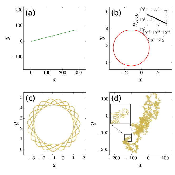
Figure 1: Swimming patterns as $\sigma_{2}$ increases (growth rate of second harmonic). (a) Straight ($\sigma_{2}=-1$), (b) circular ($\sigma_{2}=0.1$; inset shows scaling of circle radius close to criticality confirming prediction (Eq. (26)) , (c) precession ($\sigma_{2}=0.4$), and (d) chaotic trajectories ($\sigma_{2}=1.2$).

Numerical solution of (19b)-(19c) reveals a complex dynamics ranging from straight trajectories to chaotic ones. To illustrate this, we have set all parameters to unity, and varied $\sigma_{2}$ from negative to positive (by keeping $\sigma_{2}$ small enough for higher order harmonics to play a minor role).

Figure 1 shows a typical swimming pattern, going from straight, circular, precession, to an apparently erratic motion. This last motion (chaos) bears strong resemblance with the run-tumble dynamics, having a persistent random walk feature. We measure the mean square displacement

$$\mbox{MSD}(\tau)=\langle\Delta x^{2}(\tau)\rangle=\langle\|\mathbf{x}(t+\tau)-\mathbf{x}(t)\|^{2}\rangle,$$

where $\mathbf{x}(t)$ is the location of the particle at time $t$ and $\langle\cdot\rangle$ denotes the average along the entire trajectory. Figure 2 reports the MSD. At short time we have a ballistic motion, whereas for longer times, a de-correlation process due to chaotic turns of velocity direction leads to a MSD proportional to ${\tau}^{\kappa}$, where $\kappa$ depends on model parameters, yielding both diffusive and sub-diffusive regimes (Fig. 2 ). Actulally, it is not obvious that a chaotic motion is equivalent (at long time) to normal diffusion. There are several chaotic maps yielding anomalous diffusion Geisel and Nierwetberg (1982).

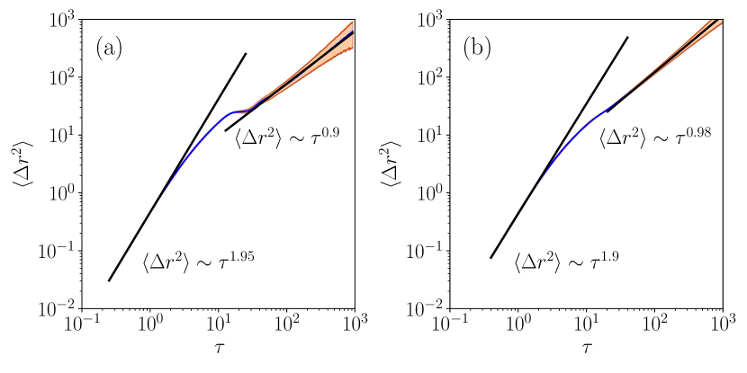
Figure 2: Mean square displacement for (a) $\sigma_{2}=1.0$ and (b) $\sigma_{2}=1.2$. The shaded region corresponds to the standard deviation in MSD.

Extension to 3D. As in 2D the 3D model relies only on two harmonics of the concentration field, $c_{i}$ and $c_{ij}$, where $c_{i}$ is a 3D vector and $c_{ij}$ is a 3D symmetric traceless tensor. The particle is taken as a unit sphere with a concentration

$$c(\bm{r})=c_{i}r_{i}+c_{ij}r_{i}r_{j}.$$ (27)

where $r_{i}$ is the ith component of position vector on the particle surface. We propose the following system (see Supplemental Materials):

$$\dot{c}_{i} =\sigma_{1}c_{i}+\alpha_{1}c_{j}^{2}c_{i}+\beta_{1}(c_{k}^{2}c_{ij}c_{j}-c_{j}c_{k}c_{jk}c_{i})$$ (28a)

$$\dot{c}_{ij} =\sigma_{2}c_{ij}+\beta_{2}(c_{i}c_{j}-\delta_{ij}c_{k}^{2}/3).$$ (28b)

All terms written above are consistent with symmetry (three rotations). System (28a,b) leaves the evolution of the norm of $c_{i}$ independent of $c_{ij}$

$$c_{i}\dot{c}_{i}=\sigma_{1}c_{i}^{2}+\alpha_{1}(c_{i}^{2})^{2}.$$ (29)

This choice is not necessary, but allows for a complete analytical handling (results are unaffected by this choice (see below).This is the classical form of a pitchfork bifurcation. We assume $\alpha_{1}<0$ (supercritical bifurcation). With this choice, we obtain that for $\sigma_{1}<0$ the stable solution is $c_{i}^{2}=0$, which corresponds to a non-motile case. For $\sigma_{1}>0$, the stable solution is

$$c_{i}^{2}=-\sigma_{2}/\alpha_{1},$$ (30)

which corresponds to a motile solution (recall that the swimming speed $v_{i}$ is proportional to $c_{i}$). Since the norm dynamics of $c_{i}$ is decoupled, we assume below that the norm of $c_{i}$ has already reached its stationary value defined by Eq. (30) (in 2D we have actually shown that for circular motion amplitudes $\rho_{1}$ and $\rho_{2}$ are constants). As we have seen in 2D a circular trajectory leads to a fixed concentration spot moving along the particle periphery. Instead of using the dynamics of phases ($\phi_{1}$ and $\phi_{2}$) as in 2D, we find it more convenient in 3D to follow another approach. The idea is to find if there is a co-rotating frame in which the concentration spot would be steady. Rotation of a spot along the sphere requires some symmetry-breaking. For the straight motion (say along $x$) the spot possesses axial symmetry around that axis. A first obvious breaking of this symmetry leaves a single mirror of symmetry containing $x$-axis; we take it to be $x-y$ plane. We will see that the concentration spot will spontaneously move along the equator, and the particle will follow a circular path. The next broken symmetry is the $x-y$ mirror, which will make the spot to move along a closed trajectory, distinct from equator, and the particle follows a helical path. It is convenient to solve our system (28a)-(28b) in the co-moving frame with angular velocity ${\bm{\omega}}$ (to be determined) of concentration spot. The left hand side of (28a)-(28b) become (see SI ) $\dot{c}_{i}+\varepsilon_{ijk}\omega_{j}c_{k}$ ($\varepsilon$ is Levi-Civita symbol) and $\dot{c}_{ij}+\varepsilon_{ikl}\omega_{k}c_{kj}+\varepsilon_{jkl}\omega_{k}c_{ki}$. Then setting $\omega_{i}=\beta_{1}\varepsilon_{ijk}c_{j}c_{kl}c_{l}$ cancels $\beta_{1}$ term in (28a), and we are then left with equation of $c_{ij}$ only.

We first consider the case with $c_{xz}=c_{yz}=0$ (we assume $x-y$ plane symmetry). The only non-zero $\omega_{i}$ is $\omega_{z}=\beta_{1}c_{j}^{2}c_{xy}$. Analysis of $c_{xy}$ equation shows a stable nontrivial fixed point for $(c_{i}^{2})^{2}>\sigma_{2}^{2}/(\beta_{1}\beta_{2})$. Because only $\omega_{z}\neq 0$ the spot rotates along the equator (and so does vector $c_{i}$), and the particle follows a circular path. We subsequently analyze linear stability of this solution (see SI ), by allowing modes breaking $x-y$ mirror symmetry (meaning $c_{xz}$ and $c_{yz}$ non zero). A straightforward eigenvalue problem shows that $x-y$ mirror symmetry is lost for $(c_{i}^{2})^{2}>3\sigma_{2}^{2}(\beta_{1}\beta_{2})$, and we find (besides $\omega_{z}$) $\omega_{x}=\beta_{1}c_{i}^{2}c_{yz}$ (an appropriate choice of $z$-axis allows to set $c_{xz}=0$), meaning that as soon as $c_{yz}\neq 0$, the spot moves along a circle different from equator and the particle follows a helical path (Fig. 3).

To highlight the genericity of the presented results, we write below the evolution equations for the first and second harmonics based on symmetry only (invariance under 3D rotations), without adopting the special form (28b) expressed by the $\beta_{1}$ term. To the leading order we have

$$\dot{c}_{i} =\sigma_{1}c_{i}+\alpha_{1}c_{j}^{2}c_{i}+\beta_{1}c_{ij}c_{j}$$ (31a)

$$\dot{c}_{ij} =\sigma_{2}c_{ij}+\beta_{2}(c_{i}c_{j}-\delta_{ij}c_{k}^{2}/3).$$ (31b)

Figure 3 shows the full numerical result of this model which captures the analytical results.

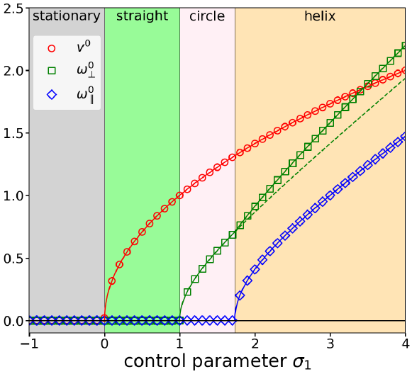
Figure 3: Top: Bead velocity showing series of bifurcations from straight, circular to helical motion.The components of angular velocity along the velocity and orthogonal to it are shown as $\omega_{\parallel}^{0}$ and $\omega_{\bot}^{0}$, respectively. Solid lines refer to analytical solution and symbols to numerical ones. Bottom: Bead trajectory showing helical path and a concentration spot following a circle (white) outside the equator.

Before concluding this section, some remarks are in order. We have written here the two harmonic equations based on symmetries. We have shown how to derive in 2D the two harmonic equations from an explicit phoretic model (more details can be found in Farutin et al. (2021), exhibiting both qualitative and quantitative agreements with the full model). The same strategy could be adopted in 3D without additional conceptual complications. Our goal was to highlight that two harmonics are sufficient to capture the essential features, and that symmetries can dictate the general form of the equations. The structure of the explicit phoretic model adopted here calls for an important remark, however. For the 3D version of the phoretic model adopted here, it has been shown by Rednikov et al.Rednikov et al. (1994) and by Morozov and Michelin Morozov and Michelin (2019b) that the swimming speed $V_{0}$ does not behave as the square root with distance from threshold (as follows from our study), but has a linear behavior. More precisely, for $Pe<Pe_{1}$, $V_{0}=0$ and $\lvert V_{0}\rvert\sim Pe-Pe_{1}$ for $Pe>Pe_{1}$. We note in passing that Morozov and Michelin Morozov and Michelin (2019b) called this bifurcation trancritical, but in fact this is still a pitchfork bifurcation, albeit non classical, since the solution $V_{0}=0$ becomes unstable for $Pe>Pe_{1}$ in favor of two symmetric solutions, $V_{0}\sim\pm(Pe-Pe_{1})$. We should refer to this bifurcation as a singular pitchfork bifurcation; it is definitely not a transcritical bifurcation Morozov and Michelin (2019b) which requires that a fixed point branch (here the non motile state) exchanges its stability with the other fixed point branch (motile state) at their crossing junction. We have considered recently a simplified version of the phoretic model and found an exact analytical solution Farutin and Misbah (2021) which confirms the singular nature, in that $\lvert V_{0}\rvert\sim Pe-Pe_{1}$ for $Pe>Pe_{1}$. We have shown that this singular behavior occurs only for an infinite system size (be it in 2D or 3D), whereas for a finite size (but arbitrary large) the bifurcation is a classical pitchfork bifurcation, in that $V_{0}\sim({Pe-Pe_{1}})^{1/2}$. This implies that our spirit of regular expansion in power series of harmonic amplitudes ($C_{1}$ and $C_{2}$) is legitimate for a finite size. In addition, we have shown that the singular behavior for infinite size is only present in the particular phoretic model presented here and considered by Rednikov et al.Rednikov et al. (1994) and Morozov and Michelin Morozov and Michelin (2019b). Indeed, if a slightly different version of the model is adopted Farutin and Misbah (2021), in which it is supposed that the emitted solute is, besides advection and diffusion, consumed at a certain frequency (giving rise, for example, to some product, not necessarily for interest), then the singular nature of the bifurcation for infinite systems is suppressed (even for an infinitesimal consumption rate); the bifurcation becomes of classical pitchfork bifurcation. Nevertheless, the works of Rednikov et al.Rednikov et al. (1994) and Morozov and Michelin Morozov and Michelin (2019b) have a merit of pointing out a non trivial singular nature of bifurcation, rarely encountered in classical nonequlibrium systems undergoing bifurcations (such as Bénard and Marangoni convection, Turing systems, crystal growth… which have been a focus of nonlinear community for decades). The singular nature of the bifurcation means that the radius of convergence of expansions in powers of amplitudes of harmonics goes to zero at the bifurcation point. This raises an important question of how to properly cope a priori, for a given nonlinear model, with the existence of singular bifurcations in a proper manner. We have provided very recently a framework along this line Farutin and Misbah (2021).

Conclusion. The model has identified the fact that locomotory complexity leading to diverse trajectories can be captured on the basis of symmetries and nonlinear interactions, lending evidence to its universality. The model can be adopted for any motion fueled by a chemical field, a prominent and vast field of research is mammalian cell motility, which is known to be dictated by myosin and actin kinetics. The model can be effective not only for spherically shaped motile entities, but also for any shape as long as the shape of the cell can be reconstructed from the chemical field. The model can also find application in embryonic development. Underlying the multicellular choreography is the actomyosin cytoskeleton dynamics, leading to the propagation of localized concentration pulsesNegro, G. et al. (2019); Blanchard et al. (2018) affecting cell rearrangement. This study also opens up new perspectives to tackle motility from a novel angle. Indeed, it should incite analytical derivation of simple nonlinear equations (as studied here) from different explicit examples of motility. This will allows linking the phenomenological coefficients used here to biophysical and chemical parameters of a motile system, in order to determine the conditions of manifestation, or the lack thereof, of complex motions in parameter space, without resorting to the computationally expensive solution of the full basic model, which involves reaction-diffusion-advection with long range hydrodynamics.

We thank CNES (Centre National d’Etudes Spatiales) (C.M. S. M. R. and A.F.) for a financial support and for having access to experimental data, and the French-German university program ”Living Fluids” (grant CFDA-Q1-14) (C.M., A.F. and S. R.) for a financial support

References

- Barry and Bretscher (2010) Nicholas P Barry and Mark S Bretscher, “Dictyostelium amoebae and neutrophils can swim,” Proceedings of the National Academy of Sciences 107, 11376–11380 (2010).
- O’Neill et al. (2018) Patrick R. O’Neill, Jean A. Castillo-Badillo, Xenia Meshik, Vani Kalyanaraman, Krystal Melgarejo, and N. Gautam, “Membrane flow drives an adhesion-independent amoeboid cell migration mode,” Developmental Cell 46, 9 – 22.e4 (2018).
- Farutin et al. (2019) A. Farutin, J. Etienne, C. Misbah, and P. Récho, “Crawling in a fluid,” Phys. Rev. Lett. 123, 118101 (2019).
- Aoun et al. (2020) Laurene Aoun, Paulin Negre, Alexander Farutin, Nicolas Garcia-Seyda, Mohd Suhail Rivzi, Remi Galland, Alphee Michelot, Xuan Luo, Martine Biarnes-Pelicot, Claire Hivroz, Salima Rafai, Jean-Baptiste Sibareta, Marie-Pierre Valignat, Chaouqi Misbah, and Olivier Theodoly, “Mammalian amoeboid swimming is propelled by molecular and not protrusion-based paddling in lymphocytes,” Biophys. J. 119, 1157–1177 (2020).
- Mori et al. (2020) Francesco Mori, Pierre Le Doussal, Satya N. Majumdar, and Grégory Schehr, “Universal survival probability for a -dimensional run-and-tumble particle,” Phys. Rev. Lett. 124, 090603 (2020).
- Angelani et al. (2014) L Angelani, R Di Leonardo, and M Paoluzzi, “First-passage time of run-and-tumble particles,” The European Physical Journal E 37, 59 (2014).
- Rupprecht et al. (2016) Jean-Fran çois Rupprecht, Olivier Bénichou, and Raphael Voituriez, “Optimal search strategies of run-and-tumble walks,” Phys. Rev. E 94, 012117 (2016).
- Bénichou et al. (2011) O. Bénichou, C. Loverdo, M. Moreau, and R. Voituriez, “Intermittent search strategies,” Rev. Mod. Phys. 83, 81–129 (2011).
- Polin et al. (2009) Marco Polin, Idan Tuval, Knut Drescher, J. P. Gollub, and Raymond E. Goldstein, “Chlamydomonas swims with two “gears” in a eukaryotic version of run-and-tumble locomotion,” Science 325, 487–490 (2009), https://science.sciencemag.org/content/325/5939/487.full.pdf .
- Jennings (1901) H. S. Jennings, “On the significance of spiral swimming of organisms,” Am. Soc. Natural. 35, 369 (1901).
- Riedel et al. (2005) Ingmar H. Riedel, Karsten Kruse, and Jonathon Howard, “A self-organized vortex array of hydrodynamically entrained sperm cells,” Science 309, 300–303 (2005), https://science.sciencemag.org/content/309/5732/300.full.pdf .
- Jana et al. (2012) Saikat Jana, Soong Ho Um, and Sunghwan Jung, “Paramecium swimming in capillary tube,” Physics of fluids 24, 041901 (2012).
- Berg (1993) Howard C Berg, Random walks in biology (Princeton University Press, 1993).
- Cates and Tailleur (2013) Michael E Cates and Julien Tailleur, “When are active brownian particles and run-and-tumble particles equivalent? consequences for motility-induced phase separation,” EPL (Europhysics Letters) 101, 20010 (2013).
- Shenoy et al. (2007) V. B. Shenoy, D. T. Tambe, A. Prasad, and J. A. Theriot, “A kinematic description of the trajectories of listeria monocytogenes propelled by actin comet tails,” Proceedings of the National Academy of Sciences 104, 8229–8234 (2007).
- Krüger et al. (2016) Carsten Krüger, Gunnar Klös, Christian Bahr, and Corinna C Maass, “Curling liquid crystal microswimmers: A cascade of spontaneous symmetry breaking,” Phys. Rev. Lett. 117, 048003 (2016).
- Löwen (2016) Hartmut Löwen, “Chirality in microswimmer motion: From circle swimmers to active turbulence,” The European Physical Journal Special Topics 225, 2319–2331 (2016).
- Suga et al. (2018) Mariko Suga, Saori Suda, Masatoshi Ichikawa, and Yasuyuki Kimura, “Self-propelled motion switching in nematic liquid crystal droplets in aqueous surfactant solutions,” Phys. Rev. E 97, 062703 (2018).
- Narinder et al. (2018a) Narinder Narinder, Clemens Bechinger, and Juan Ruben Gomez-Solano, “Memory-induced transition from a persistent random walk to circular motion for achiral microswimmers,” Phys. Rev. Lett. 121, 078003 (2018a).
- Izri et al. (2014) Ziane Izri, Marjolein N Van Der Linden, Sébastien Michelin, and Olivier Dauchot, “Self-propulsion of pure water droplets by spontaneous marangoni-stress-driven motion,” Phys. Rev. Lett. 113, 248302 (2014).
- Hu et al. (2019) W. F. Hu, T. S. Lin, S. Rafai, and C. Misbah, “Chaotic swimming of phoretic particles,” Phys. Rev. Lett. 123, 238004 (2019).
- Lauga et al. (2006) E. Lauga, W. R. DiLuzio, G. M. Whitesides, and H. A. Stone, “Swimming in circles: Motion of bacteria near solid boundaries,” Biophys. J.. 105, 069401 (2006).
- Michelin et al. (2013) S. Michelin, E. Lauga, and D. Bartolo, “Spontaneous autophoretic motion of isotropic particles,” Phys. Fluids 25, 061701 (2013).
- Morozov and Michelin (2019a) Matvey Morozov and Sébastien Michelin, “Nonlinear dynamics of a chemically-active drop: From steady to chaotic self-propulsion,” The Journal of chemical physics 150, 044110 (2019a).
- Schmitt and Stark (2013) Maximilian Schmitt and Holger Stark, “Swimming active droplet: A theoretical analysis,” EPL (Europhysics Letters) 101, 44008 (2013).
- Hawkins et al. (2011) Rhoda J Hawkins, Renaud Poincloux, Olivier Bénichou, Matthieu Piel, Philippe Chavrier, and Raphaël Voituriez, “Spontaneous contractility-mediated cortical flow generates cell migration in three-dimensional environments,” Biophysical journal 101, 1041–1045 (2011).
- Callan-Jones et al. (2016) A. C. Callan-Jones, V. Ruprecht, S. Wieser, C. P. Heisenberg, and R. Voituriez, “Cortical flow-driven shapes of nonadherent cells,” Phys. Rev. Lett. 116, 028102 (2016).
- Sondak et al. (2016) D. Sondak, C. Hawley, S. Heng, R. Vinsonhaler, E. Lauga, and J.-L. Thiffeault, “Can phoretic particles swim in two dimensions?” Phys. Rev. E 94, 062606 (2016).
- Blake (1971) J.R. Blake, “Self propulsion due to oscillations on the surface of a cylinder at low reynolds number,” Bulletin of the Australian Mathematical Society 5, 255–264 (1971).
- Farutin et al. (2021) Alexander Farutin, Mohd Suhail Rizvi, Wei Fan Hu, Te Sheng Lin, Salima Rafai, and Chaouqi Misbah, “A reduced model for a phoretic swimmer,” arXiv:2112.12023 (2021).
- (31) See supplemental material at [URL will be inserted by publisher] .
- Narinder et al. (2018b) N Narinder, Clemens Bechinger, and Juan Ruben Gomez-Solano, “Memory-induced transition from a persistent random walk to circular motion for achiral microswimmers,” Phys. Rev. Lett. 121, 078003 (2018b).
- Geisel and Nierwetberg (1982) T. Geisel and J. Nierwetberg, “Onset of diffusion and universal scaling in chaotic systems,” Phys. Rev. Lett. 48, 7–10 (1982).
- Rednikov et al. (1994) Alexei Ye Rednikov, Yuri S Ryazantsev, and Manuel G Velarde, “Drop motion with surfactant transfer in a homogeneous surrounding,” Physics of Fluids 6, 451–468 (1994).
- Morozov and Michelin (2019b) Matvey Morozov and Sébastien Michelin, “Self-propulsion near the onset of marangoni instability of deformable active droplets,” Journal of Fluid Mechanics 860, 711–738 (2019b).
- Farutin and Misbah (2021) Alexandr Farutin and Chaouqi Misbah, “Singular bifurcations: a regularization theory,” arXiv:2112.12094 (2021).
- Negro, G. et al. (2019) Negro, G., Lamura, A., Gonnella, G., and Marenduzzo, D., “Hydrodynamics of contraction-based motility in a compressible active fluid,” EPL 127, 58001 (2019).
- Blanchard et al. (2018) Guy B Blanchard, Jocelyn Étienne, and Nicole Gorfinkiel, “From pulsatile apicomedial contractility to effective epithelial mechanics,” Current Opinion in Genetics & Development 51, 78 – 87 (2018), developmental mechanisms, patterning and evolution.