Abstract

. Multi-jet production at the LHC is an important process to study. In particular, events with final state kinematic configurations where we have two jets widely separated in rapidity with similar $p_{T}$ and lots of mini-jets or jets populating the space in between are relevant for the high energy limit of QCD. Keeping the jet multiplicity fixed, the study of these events is a good ground to test different models of multi-particle production in hadron-hadron collisions. We report on a comparison between the predictions of the old multiperipheral Chew-Pignotti model and those of BFKL for the single jet rapidity distributions and for jet-jet rapidity correlations.

1 Introduction

An important question in Quantum Chromodynamics (QCD) is the structure of the high energy limit dynamics of multi-particle production at hadron and hadron-lepton colliders. Multi-particle events, and in particular, multi-jet events, are difficult to describe when one wants to go beyond the leading order (LO) approximation in fixed order perturbation theory. Even in the early days of hadron colliders (Intersecting Storage Rings, ISR at CERN) when the colliding energy was of the order of few tens of GeV and QCD was not yet the established theory of the strong interaction, multi-particle production was one of the key problems to tackle in order to probe the underlying dynamics even on heuristic terms. The experimental data amassed in the last 50-60 years, starting from those early attempts, have generally reinforced the view that the final state particles (pions, kaons, protons, etc) that end up on the detector seem to belong in correlated “clusters” Dremin:1977wc that are emitted in the hard scattering part of the process or on the partonic level.

Our modern day picture of a generic partonic cross section of two incoming partons that interact and produce two or more outgoing partons which in turn, through a parton shower, radiate new quarks and gluons and form jets does not contradict the heuristic notion of clusters. The study of differential distributions and particle-particle correlations between final states had given important insights about the strong interaction no matter whether the final states were considered before hadronizations effects (final state partons/jets) or after (hadrons in the detector calorimeters). Especially for jets, correlations summarize important properties without being too sensitive to unresolved soft particles in the jet Tannenbaum:2005by (see also the introduction of Ref. SanchisLozano:2008te ). It is thus very interesting to see whether the rapidity distributions of final state hadrons are any similar to the rapidity distributions of jets.

Quite a few different approaches exist that are useful to probe multi-particle hadroproduction beyond fixed order. These are resummation frameworks that resum different leading contributions to amplitudes (e.g. DGLAP Gribov:1972ri ; Gribov:1972rt ; Lipatov:1974qm ; Altarelli:1977zs ; Dokshitzer:1977sg , BFKL Kuraev:1977fs ; Kuraev:1976ge ; Fadin:1975cb ; Lipatov:1976zz ; Balitsky:1978ic ; Lipatov:1985uk , CCFM Ciafaloni:1987ur ; Catani:1989yc , Linked Dipole Chain Gustafson:1986db ; Gustafson:1987rq ; Andersson:1995ju , Lund Model Andersson:1998tv , see also LHCForwardPhysicsWorkingGroup:2016ote ).

The run 2 of the LHC at 13 TeV has provided lots of data which should be analyzed in detail. Here, we want to focus on a final state configurations which could be quite important to answer the question of what is the range of applicability of different multi-particle production models. These configurations correspond to events with several final state jets where the two outermost in rapidity ones are also well separated in rapidity and can be tagged requiring that their transverse momenta are similar and genaraly large. These corresponds to a subset of the so-called Mueller-Navelet jets Mueller:1986ey and if additionally we require a very similar $p_{T}$ for the outermost jets (however, not within overlapping ranges) we can enforce that their influence on the rapidity distributions of the jets in between will be symmetric.

Our aim here is to report on our recent work deLeon:2020myv where we studied some of the characteristics that can be attributed to these processes. As the most striking features in multiperipheral models can be found in the rapidity space –the origin of these features can be traced at the decoupling of the transverse degrees of freedom from the longitudinal ones–, we will present single rapidity differential distributions and two-jet rapidity-rapidity correlations.

Assuming configurations in a hadron-hadron collider with fixed final state jet multiplicity $N$, the single and double rapidity distributions for a given jet and a pair of jets are given respectively by $\rho_{1}(y_{i})$ and $\rho_{2}\left(y_{i},y_{j}\right)$, where $i$ and $j$ are the positions of the jets once they are ordered in rapidity with $1\leq i,j\leq N$. We can formally define for the single and double differential normalized distributions

$$\rho_{1}(y_{i})=\frac{1}{\sigma}\int d^{2}p_{\perp}\frac{d^{3}\sigma}{dy_{i}d^{2}p_{\perp i}}$$ (1)

and

$$\rho_{2}\left(y_{i},y_{j}\right)=\frac{1}{\sigma}\int d^{2}p_{\perp i}d^{2}p_{\perp j}\frac{d^{6}\sigma}{dy_{i}d^{2}p_{\perp i}dy_{j}d^{2}p_{\perp j}}\,.$$ (2)

After integrating over their transverse components we will have

$$\rho_{1}(y_{i})=\frac{1}{\sigma}\frac{d\sigma}{dy_{i}}$$ (3)

and

$$\rho_{2}\left(y_{i},y_{j}\right)=\frac{1}{\sigma}\frac{d^{2}\sigma}{dy_{i}dy_{j}}\,.$$ (4)

The two-particle rapidity-rapidity correlation function is then given by

$$C_{2}\left(y_{i},y_{j}\right) = \frac{1}{\sigma}\frac{d^{2}\sigma}{dy_{i}dy_{j}}-\frac{1}{\sigma^{2}}\frac{d\sigma}{dy_{i}}\frac{d\sigma}{dy_{j}}$$ (5)

$$= \rho_{2}\left(y_{i},y_{j}\right)-\rho_{1}(y_{i})\rho_{1}(y_{j})$$ (6)

In practice however, the correlation function is usually computed with the following expression which is less sensitive to experimental errors:

$$R_{2}\left(y_{1},y_{2}\right)=\frac{C_{2}\left(y_{1},y_{2}\right)}{\rho_{1}\left(y_{1}\right)\rho_{1}\left(y_{2}\right)}=\frac{\rho_{2}\left(y_{1},y_{2}\right)}{\rho_{1}\left(y_{1}\right)\rho_{1}\left(y_{2}\right)}-1\,.$$ (7)

In Section 2, we calculate the analytic expressions for the double and single rapidity distributions within an old multiperipheral model, namely the Chew-Pignotti model Chew:1968fe , wehreas, In Section 3, we explain how we compute the same quantities for the gluon Green’s function of a collinear BFKL model by using Monte Carlo techniques. We conclude in Section 4.

2 The Chew-Pignotti Model

As we mentioned in the introduction, we will work with a Chew-Pignotti type of multiperipheral model Chew:1968fe following the analysis by DeTar in Ref. Detar:1971qw . The simplified features of the model will give us the opportunity to produce analytic results that could in principle be compared to the experimental data. For a more detailed review on multiperipheral models and the cluster concept in multiparticle production at hadron colliders, see Ref. Dremin:1977wc and references therein. The key point is that in these types of models, the transverse coordinates decouple from the longitudinal degrees of freedom (rapidity) and that is what allows to obtain analytic expressions for the rapidity distributions.

While the multiperipheral models were devised to describe multiple particle production, we will use the Chew-Pignotti here for multiple jet production. We will assume that the rapidity separation of the the bounding jets is Y and also that the jets in between have a fixed multiplicity $N$ such that in total we will have $N+2$ final state jets in each event. The outermost in rapidity jets (the most forward/backward jets) are having rapidities $\pm\frac{Y}{2}$. It should be clear that we choose to work with limits $y_{0}=-\frac{Y}{2}$ and $y_{N+1}=\frac{Y}{2}$ because we want to cast our analytic expressions for the distributions in a symmetric way with respect to the forward and backward rapidity direction. Naturally, one could also work with limits $y_{0}=0$ and $y_{N+1}=Y$. Actually for the results from the BFKL approach in section 3, we choose to present our plots in the range $\left[0,Y\right]$ as we want to be closer to an experimental analysis setup.

The cross section for the production of $N+2$ final state jets is given by

$$\sigma_{N+2} = \alpha^{N+2}\int_{0}^{Y}\prod_{i=1}^{N+1}dz_{i}\delta\left(Y-\sum_{s=1}^{N+1}z_{s}\right)$$ (8)

$$= \alpha^{N+2}\int_{-\frac{Y}{2}}^{\frac{Y}{2}}dy_{N}\int_{-\frac{Y}{2}}^{y_{N}}dy_{N-1}\cdots\int_{-\frac{Y}{2}}^{y_{3}}dy_{2}\int_{-\frac{Y}{2}}^{y_{2}}dy_{1}\,=\,\alpha^{2}\frac{\left(\alpha Y\right)^{N}}{N!}\,,$$

which leads to a total cross section $\sigma_{\rm total}=\sum_{N=0}^{\infty}\sigma_{N+2}=\alpha^{2}e^{\alpha Y}$ and the rise with $Y$ would need to be tamed by introducing unitarity corrections in transverse space. A rapidity $y_{l}$, with $l=0,\dots,N+1$ is assigned to each of the final-state jets. At $y_{0}=-\frac{Y}{2}$ and $y_{N+1}=\frac{Y}{2}$ we have the positions of the outermost jets with the jet vertex reduced to a simple factor equal to $\alpha$, the strong coupling constant. The in-between jets will have rapidities $y_{l}=-\frac{Y}{2}+\sum_{j=1}^{l}z_{j}$, where $l=1,\dots N$.

We are mainly interested in the description of the differential distributions for events with fixed final state multiplicity, firstly on a qualitative level. At this point we need to note the following: the final jet multiplicity for a given final state is uniquely defined, it actually depends on the lower $p_{T}$ cutoff we set for a mini-jet to qualify as a jet as well as on the chosen jet radius $R$ (in the rapidity-azimuthal angle plane) for the jet clustering algorithm. Nevertheless, we believe that our analysis in the following is valid once a well defined mechanism for deciding the multiplicity of a final state is established. This is not a trivial statement at is it implies that if a final state has initially been assigned multiplicity $N_{1}+2$ complies with the $N_{1}+2$ differential distributions, then, if a different set of parameters is chosen for the jet clustering algorithm which results in a different number of final state jets giving a shift in multiplicity from $N_{1}$ to $N_{2}$, then that final state will also comply with the $N_{2}+2$ differential distributions.

The contribution for jet $l$ in a $N+2$ final state event, will have the following differential distribution in rapidity

$$\frac{d\sigma_{N+2}^{(l)}}{dy_{l}} = \alpha^{N+2}\int_{0}^{Y}\prod_{i=1}^{N+1}dz_{i}\delta\left(Y-\sum_{s=1}^{N+1}z_{s}\right)\delta\left(y_{l}+\frac{Y}{2}-\sum_{j=1}^{l}z_{j}\right)$$ (9)

$$= \alpha^{N+2}\int_{y_{l}}^{\frac{Y}{2}}dy_{N}\int_{y_{l}}^{y_{N}}dy_{N-1}\cdots\int_{y_{l}}^{y_{l+2}}dy_{l+1}\int_{-\frac{Y}{2}}^{y_{l}}dy_{l-1}\cdots\int_{-\frac{Y}{2}}^{y_{3}}dy_{2}\int_{-\frac{Y}{2}}^{y_{2}}dy_{1}$$

$$= \alpha^{N+2}\frac{\left(\frac{Y}{2}-y_{l}\right)^{N-l}}{(N-l)!}\frac{\left(y_{l}+\frac{Y}{2}\right)^{l-1}}{(l-1)!}\,,$$

as derived from Eq. (8). For very large multiplicities this results to an asymptotic Poisson distribution as one can verify, e.g., in the region $y\simeq-\frac{Y}{2}$ with $y=\left(\frac{\lambda}{N}-\frac{1}{2}\right)Y$ where

$$\lim_{N\to\infty}{N-1\choose l-1}\left(1-\frac{\lambda}{N}\right)^{N-l}\left(\frac{\lambda}{N}\right)^{l-1} = e^{-\lambda}\frac{\lambda^{l-1}}{(l-1)!}\,.$$ (10)

Taking the limits $l\to 1$ and $y_{l}\to-\frac{Y}{2}$ in Eq. (9) we derive a normalized universal distribution for each $N$ when plotted versus $2y/Y$. The case for N=7+2 is plotted in Fig. 1 (left) which is very characteristic for multiperipheral models. We remind the reader that the notation jet_i=1,2,…,N is introduced for jets with ordered rapidities $y_{1}<y_{2}<\dots<y_{N}$.

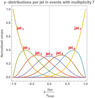
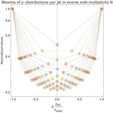
Figure 1: Rapidity distributions for each of the jets in a final state with seven mini-jets (left). Their maxima are indicated by the symbol \tiny7⃝ (right). The positions of the $y$-distribution maxima in configurations with multiplicity $N$ are marked by \tinyN⃝ (right).

All these seven normalized $y$-distributions (one for each of the seven jets) spans an area of $\frac{2}{N}$. Their maxima are found at $y=\frac{2l-N-1}{2(N-1)}Y$ with a value that is

$${N-1\choose l-1}\frac{(l-1)^{l-1}}{(N-1)^{N-1}}\left(N-l\right)^{N-l}\,.$$ (11)

In Fig. 1 (right), we show the maxima for multiplicities $N$, where $\left(3+2\right)\leq\left(N+2\right)\leq\left(15+2\right)$.

In a similar manner, we get expressions for the double differential rapidity distributions for jet pairs, i.e.

$$\frac{d^{2}\sigma_{N+2}^{(l,m)}}{dy_{l}dy_{m}} = \alpha^{N+2}\int_{0}^{Y}\prod_{i=1}^{N+1}dz_{i}\delta\left(Y-\sum_{s=1}^{N+1}z_{s}\right)\delta\left(y_{l}+\frac{Y}{2}-\sum_{j=1}^{l}z_{j}\right)\delta\left(y_{m}+\frac{Y}{2}-\sum_{k=1}^{m}z_{k}\right)$$ (12)

$$= \alpha^{N+2}\frac{\left(\frac{Y}{2}-y_{l}\right)^{N-l}}{(N-l)!}\frac{(y_{l}-y_{m})^{l-m-1}}{(l-m-1)!}\frac{\left(y_{m}+\frac{Y}{2}\right)^{m-1}}{(m-1)!}\,.$$

To calculate the correlation between the rapidities of jet $l$ and jet $m$ we use Eq. (7), more precisely

$${\cal R}_{N+2}\left(x_{l},x_{m}\right)=\sigma_{N+2}\frac{\frac{d^{2}\sigma_{N+2}^{(l,m)}}{dy_{l}dy_{m}}}{\frac{d\sigma_{N+2}^{(l)}}{dy_{l}}\frac{d\sigma_{N+2}^{(m)}}{dy_{m}}}-1=\frac{2^{N}}{N!}\frac{(N-m)!(l-1)!}{(l-m-1)!}\frac{(x_{l}-x_{m})^{l-m-1}}{\left(1+x_{l}\right)^{l-1}\left(1-x_{m}\right)^{N-m}}-1\,,$$ (13)

where $Y>y_{l}>y_{m}>0$, $l>m$ and $x_{J}=2y_{J}/Y$.

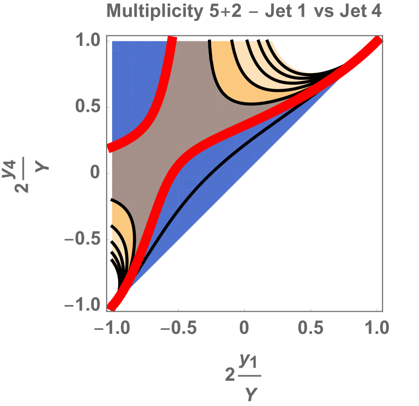
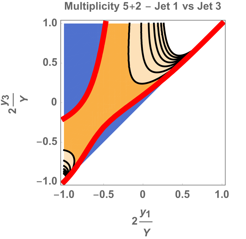
Figure 2: Left: ${\cal R}_{5+2}\left(x_{4},x_{1}\right)=\sigma_{5+2}\frac{\frac{d^{2}\sigma_{5+2}^{(4,1)}}{dy_{4}dy_{1}}}{\frac{d\sigma_{5+2}^{(4)}}{dy_{4}}\frac{d\sigma_{5+2}^{(1)}}{dy_{1}}}-1$. Right: ${\cal R}_{5+2}\left(x_{3},x_{1}\right)=\sigma_{5+2}\frac{\frac{d^{2}\sigma_{5+2}^{(3,1)}}{dy_{3}dy_{1}}}{\frac{d\sigma_{5+2}^{(3)}}{dy_{3}}\frac{d\sigma_{5+2}^{(1)}}{dy_{1}}}-1$.

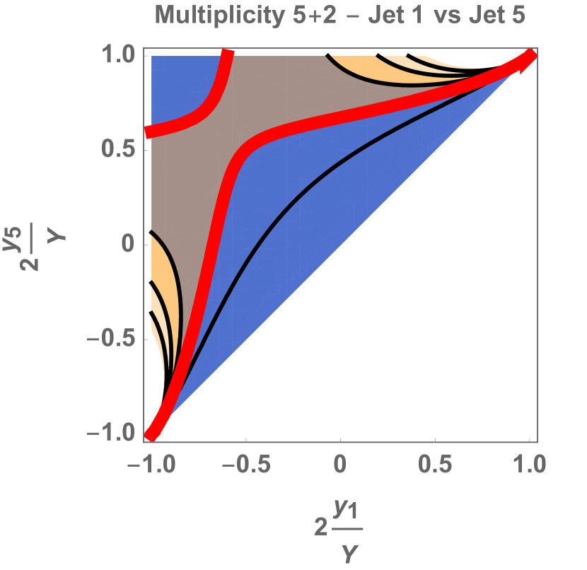
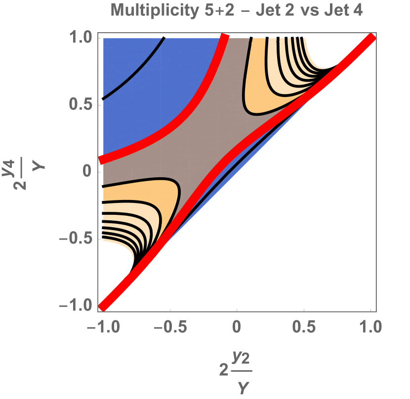
Figure 3: Left: ${\cal R}_{5+2}\left(x_{5},x_{1}\right)=\sigma_{5+2}\frac{\frac{d^{2}\sigma_{5+2}^{(5,1)}}{dy_{5}dy_{1}}}{\frac{d\sigma_{5+2}^{(5)}}{dy_{5}}\frac{d\sigma_{5+2}^{(1)}}{dy_{1}}}-1$. Right: ${\cal R}_{5+2}\left(x_{4},x_{2}\right)=\sigma_{5+2}\frac{\frac{d^{2}\sigma_{5+2}^{(4,2)}}{dy_{4}dy_{2}}}{\frac{d\sigma_{5+2}^{(4)}}{dy_{4}}\frac{d\sigma_{5+2}^{(2)}}{dy_{2}}}-1$.

We plot the correlation functions using Eq. (13) in Figs. 2 and  3. We choose multiplicity $5+2$ and we show the correlation between the rapidities of jet 1 and jet 4 (Fig. 2, left), jet 1 and jet 3 (Fig. 2, right), jet 1 and jet 5 (Fig. 3, left), jet 2 and jet 4 (Fig. 3, right). The red lines in each of them underine the contour for which ${\cal R}=0$ while the white regions correspond to sectors of very rapid growth of ${\cal R}$.

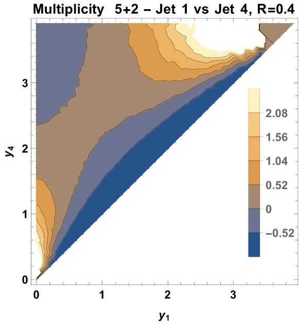
(a)

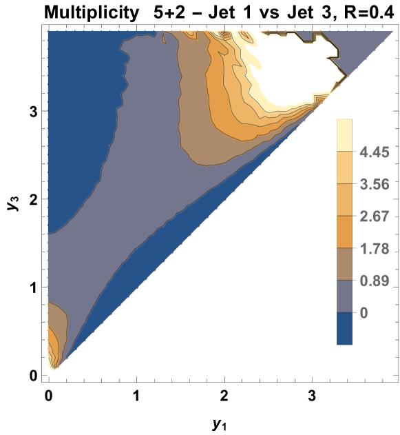
(b)

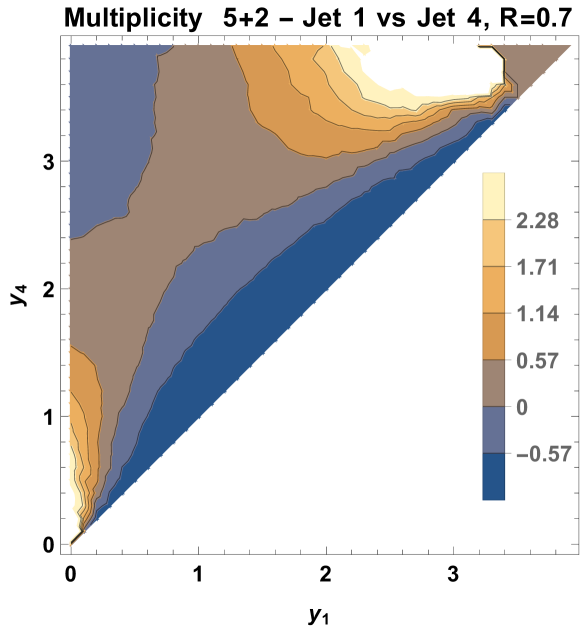
(c)

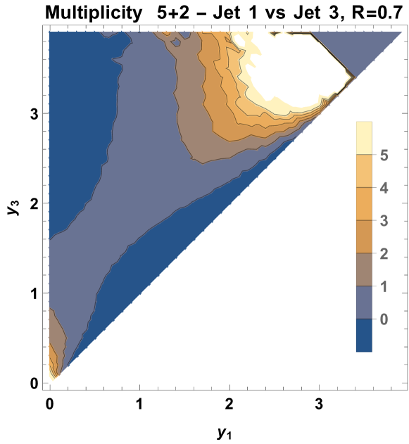
(d)

Figure 4: Top: The correlation functions of Fig. 2 with the collinear BFKL model and for jet radius $R=0.4.$ Bottom: The same but for jet radius $R=0.7$.

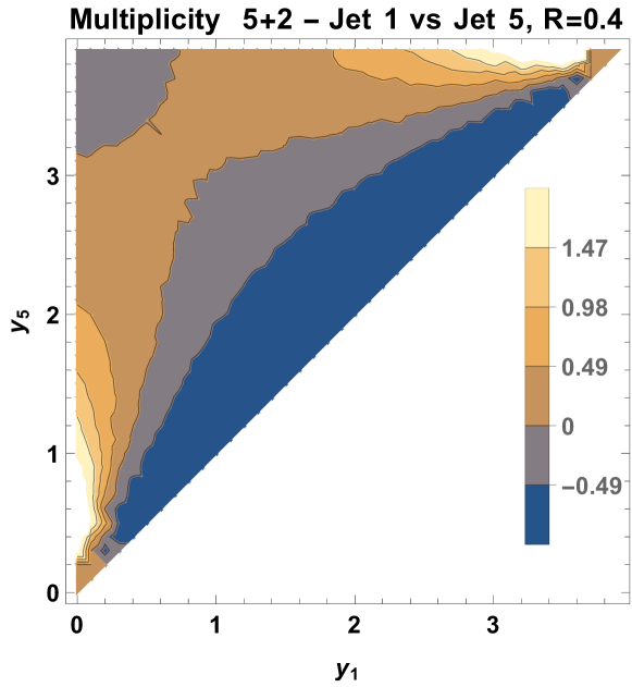
(a)

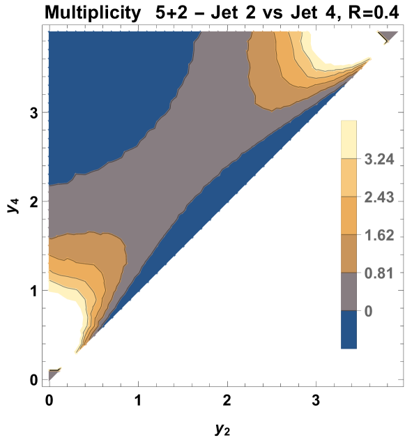
(b)

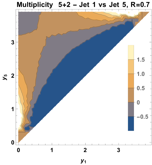
(c)

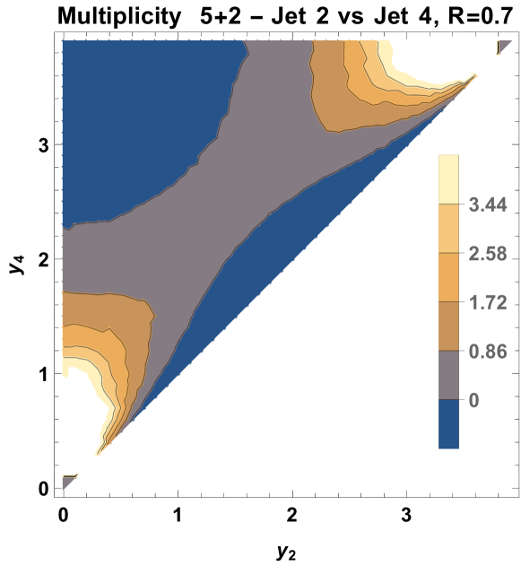
(d)

Figure 5: Top: The correlation functions of Fig. 3 with the collinear BFKL model and for jet radius $R=0.4.$ Bottom: The same but for jet radius $R=0.7$.

Our analysis here is quite simple as no relevant dynamics from the transverse coordinates of the phase space is introduced. Nevertheless, it should still be enough to capture the gross features of single rapidity distributions and double rapidity correlations which should be generally independent of the selected $p_{T}$ of the outermost in rapidity jets. In the next section, we will investigate whether these gross features are any similar to predictions derived from the BFKL formalism using a simple collinear BFKL model implemented as a special case in our Monte Carlo code BFKLex Chachamis:2011rw ; Chachamis:2011nz ; Chachamis:2012fk ; Chachamis:2012qw ; Chachamis:2015zzp ; Chachamis:2015ico ; deLeon:2021ecb .

3 Correlations in BFKL with BFKLex

In this section we evaluate the correlation functions for the rapidities of jets within the BFKL formalism. We work with the gluon Green’s function, that is at partonic level, where an emitted gluon is named a jet if its $p_{T}$ is above some cutoff and we leave for a future work the more complicated and detailed study of the full BFKL dynamics at hadronic level.

At a collider with colliding energy $s$, at the leading logarithmic approximation, where large logarithmic terms of the form ${\bar{\alpha}}_{s}^{n}\ln^{n}{s}$ are resummed (using ${\bar{\alpha}}_{s}={\bar{\alpha}}_{s}N_{c}/\pi$), the differential partonic cross section for the production of two well separated in rapidity jets and transverse momenta $\vec{p}_{i=1,2}$ is given by

$$\frac{d\hat{\sigma}}{d^{2}\vec{p}_{1}d^{2}\vec{p}_{2}} = \frac{\pi^{2}{\bar{\alpha}}_{s}^{2}}{2}\frac{f(\vec{p}_{1}^{\leavevmode\nobreak\ 2},\vec{p}_{2}^{\leavevmode\nobreak\ 2},Y)}{\vec{p}_{1}^{\leavevmode\nobreak\ 2}\vec{p}_{2}^{\leavevmode\nobreak\ 2}}\,.$$ (14)

where we take the longitudinal momentum fractions of the colliding partons to be $x_{i=1,2}$ and the rapidity difference between the two jets $Y\sim\ln{x_{1}x_{2}s/\sqrt{\vec{p}_{1}^{\leavevmode\nobreak\ 2}\vec{p}_{2}^{\leavevmode\nobreak\ 2}}}$ .

Within the BFKL resummation framework, one can show that the gluon Green’s function $f$ follows, in a collinear approximation, the integro-differential equation

$$\frac{\partial f(K^{2},Q^{2},Y)}{\partial Y} = \delta(K^{2}-Q^{2})$$ (15)

$$+\,{\bar{\alpha}}_{s}\int_{0}^{\infty}dq^{2}\left(\frac{\theta(K-q)}{K^{2}}+\frac{\theta(q-K)}{q^{2}}+4(\ln{2}-1)\delta(q^{2}-K^{2})\right)f(q^{2},Q^{2},Y)\,,$$

the solution of which can be cast in an iterative form:

$$f(K^{2},Q^{2},Y) = e^{4(\ln{2}-1){\bar{\alpha}}_{s}Y}\Bigg{\{}\delta(K^{2}-Q^{2})$$ (16)

$$+\,\sum_{N=1}^{\infty}\frac{({\bar{\alpha}}_{s}Y)^{N}}{N!}\left[\prod_{L=1}^{N}\int_{0}^{\infty}dx_{L}\left(\frac{\theta(x_{L-1}-x_{L})}{x_{L-1}}+\frac{\theta(x_{L}-x_{L-1})}{x_{L}}\right)\right]\delta(x_{N}-Q^{2})\Bigg{\}}\,.$$

Using $\delta(K^{2}-Q^{2})=\int\frac{d\gamma}{2\pi iQ^{2}}\left(\frac{K^{2}}{Q^{2}}\right)^{\gamma-1}$ and

$$\int_{0}^{\infty}dx_{N}\left(\frac{\theta(x_{N-1}-x_{N})}{x_{N-1}}+\frac{\theta(x_{N}-x_{N-1})}{x_{N}}\right)\left(\frac{x_{N}}{K^{2}}\right)^{\gamma-1}=\left(\frac{1}{\gamma}+\frac{1}{1-\gamma}\right)\left(\frac{x_{N-1}}{K^{2}}\right)^{\gamma-1},$$ (17)

which is valid for $0<\gamma<1$, we can write

$$\left[\prod_{L=1}^{N}\int_{0}^{\infty}dx_{L}\left(\frac{\theta(x_{L-1}-x_{L})}{x_{L-1}}+\frac{\theta(x_{L}-x_{L-1})}{x_{L}}\right)\right]\left(\frac{x_{N}}{K^{2}}\right)^{\gamma-1}=\left(\frac{1}{\gamma}+\frac{1}{1-\gamma}\right)^{N}$$ (18)

so that we then have

$$f(K^{2},Q^{2},Y) = \frac{e^{4(\ln{2}-1){\bar{\alpha}}_{s}Y}}{Q^{2}}\int\frac{d\gamma}{2\pi i}\left(\frac{K^{2}}{Q^{2}}\right)^{\gamma-1}\sum_{N=0}^{\infty}\frac{\left({\bar{\alpha}}_{s}Y\right)^{N}}{N!}\left(\frac{1}{\gamma}+\frac{1}{1-\gamma}\right)^{N}$$ (19)

$$= \int\frac{d\gamma}{2\pi iQ^{2}}\left(\frac{K^{2}}{Q^{2}}\right)^{\gamma-1}e^{{\bar{\alpha}}_{s}Y\chi\left(\gamma\right)}\,,$$

with $\chi(\gamma)=4(\ln{2}-1)+\gamma^{-1}+(1-\gamma)^{-1}$.

From a simple inspection of Eq. 16 one can infer that for the class of jet-jet rapidity correlations we studied in the Section 2, the predictions from this collinear BFKL model should be very similar to those in the Chew-Pignotti simple model. Actually, in Eq. (16) every $N$ increase by one unit accounts for the emission of a new final state gluon. After making use of Eq. (8), we can write

$$f(K^{2},Q^{2},Y) = \sum_{N=0}^{\infty}{\bar{\alpha}}_{s}^{N}\int_{0}^{Y}\prod_{i=1}^{N+1}dz_{i}\delta\left(Y-\sum_{s=1}^{N+1}z_{s}\right)\xi^{(N)}(K^{2},Q^{2})$$ (20)

where

$$\xi^{(N)}(K^{2},Q^{2}) = \int\frac{d\gamma}{2\pi iQ^{2}}\left(\frac{K^{2}}{Q^{2}}\right)^{\gamma-1}\chi^{N}\left(\gamma\right)\,.$$ (21)

Working in a manner that follows the logic we used to obtain Eqs. (9) and (12), i.e. we get here

$$\frac{df_{N}^{(l)}(K^{2},Q^{2},Y,y_{l})}{dy_{l}} = {\bar{\alpha}}_{s}^{N}\frac{\left(\frac{Y}{2}-y_{l}\right)^{N-l}}{(N-l)!}\frac{\left(y_{l}+\frac{Y}{2}\right)^{l-1}}{(l-1)!}\xi^{(N)}(K^{2},Q^{2})\,,$$ (22)

$$\frac{df_{N}^{(l,m)}(K^{2},Q^{2},Y,y_{l},y_{m})}{dy_{l}dy_{m}} = {\bar{\alpha}}_{s}^{N}\frac{\left(\frac{Y}{2}-y_{l}\right)^{N-l}}{(N-l)!}\frac{(y_{l}-y_{m})^{l-m-1}}{(l-m-1)!}\frac{\left(y_{m}+\frac{Y}{2}\right)^{m-1}}{(m-1)!}\xi^{(N)}(K^{2},Q^{2})\,.$$ (23)

Obviously, the $\xi^{(N)}$ factor cancels out for normalized quantities and thus we end up with the same expressions as for the Chew-Pignotti model. It is important to remember at this point that the full BFKL formalism carries non-trivial dependences in rapidity, transverse momenta and azimuthal angles which need to be studied in detail in future works. Nevertheless, our findings here in rapidity space suggest that the full BFKL predictions might not be totally different from the old multiperipheral model approach.

To connect with future works, we have implemented the BFKL collinear model within our BFKLex Monte Carlo code, setting the transverse momenta of the most forward and backward jets to be 30 and 35 GeV respectively and their difference in rapidity $Y=4$. We also set the multiplicity of the emitted gluons (jets) to be $N=5+2$. We use the anti-kt jet clustering algorithm in its implementation in fastjet Cacciari:2011ma . We present results from the collinear model in Figs. 4 and 5. The jet radius was chosen to take two values, $R=0.4$ and $R=0.7$. In Fig. 4 we plot the same correlation functions as in Fig. 2 whereas in Fig. 5 the corresponding ones for Fig. 3. It is not surprising, that the collinear model results are very similar to the Chew-Pignotti ones and obviously the actual jet radius R does not affect significantly the plots. Let us also note that in Figs. 4 and 5 we kept the rapidity range from 0 to $Y$ to make the association to experimental data setups easier. Such can be found for example in relevant dijet experimental analyses for 7 TeV data from both ATLAS and CMS Aad:2011jz ; Chatrchyan:2012pb ; Aad:2014pua ; Khachatryan:2016udy .

4 Conclusions

The 13 TeV data from the run 2 of the LHC at low luminosity are suitable for various studies of multi-jet physics. Following our recent work in Ref. deLeon:2020myv , we want to suggest the investigation of a particular subset of Mueller-Navelet jet events where the outermost jets are very similar in $p_{T}$ and the jet multiplicity is kept fixed. We believe that their experimental study is interesting as it might be possible to identify features of different multi-particle production models such as those predicted by the BFKL formalism. We have presented predictions for single and double differential distributions in jet rapidity as well as the jet-jet correlation functions from an old multiperipheral model, namely the Chew-Pignotti model, using analytic expressions we obtained after performing an analysis based on the decoupling of the longitudinal and transverse coordinates. We have also presented results for the jet-jet correlation functions from a collinear BFKL model implemented in our Monte Carlo code BFKLex. In the future, we plan to perform a more complete study of these observables in high energy QCD including the full dependence on the transverse coordinates and moving from a partonic level analysis of the BFKL gluon Green’s function to the hadronic level with PDFs included and suitable phenomenological kinematic cuts.

Comments: Presented at the Low-$x$ Workshop, Elba Island, Italy, September 27–October 1 2021.

References

- (1) I. M. Dremin, C. Quigg, Science 199, 937 (1978).
- (2) M. J. Tannenbaum, J. Phys. Conf. Ser. 27, 1-10 (2005).
- (3) M. A. Sanchis-Lozano, Int. J. Mod. Phys. A 24, 4529-4572 (2009).
- (4) V. N. Gribov, L. N. Lipatov, Sov. J. Nucl. Phys. 15, 438-450 (1972) IPTI-381-71.
- (5) V. N. Gribov, L. N. Lipatov, Sov. J. Nucl. Phys. 15, 675-684 (1972).
- (6) L. N. Lipatov, Sov. J. Nucl. Phys. 20, 94-102 (1975).
- (7) G. Altarelli, G. Parisi, Nucl. Phys. B 126, 298-318 (1977).
- (8) Y. L. Dokshitzer, Sov. Phys. JETP 46, 641-653 (1977).
- (9) E. A. Kuraev, L. N. Lipatov, V. S. Fadin, Sov. Phys. JETP 45, 199-204 (1977).
- (10) E. A. Kuraev, L. N. Lipatov, V. S. Fadin, Sov. Phys. JETP 44, 443-450 (1976).
- (11) V. S. Fadin, E. A. Kuraev, L. N. Lipatov, Phys. Lett. B 60, 50-52 (1975).
- (12) L. N. Lipatov, Sov. J. Nucl. Phys. 23, 338-345 (1976).
- (13) I. I. Balitsky and L. N. Lipatov, Sov. J. Nucl. Phys. 28, 822-829 (1978)
- (14) L. N. Lipatov, Sov. Phys. JETP 63, 904-912 (1986) LENINGRAD-85-1137.
- (15) M. Ciafaloni, Nucl. Phys. B 296, 49-74 (1988).
- (16) S. Catani, F. Fiorani, G. Marchesini, Phys. Lett. B 234, 339-345 (1990).
- (17) G. Gustafson, doi:10.1016/0370-2693(86)90622-2.
- (18) G. Gustafson, U. Pettersson, Nucl. Phys. B 306, 746-758 (1988).
- (19) B. Andersson, G. Gustafson, J. Samuelsson, Nucl. Phys. B 467, 443-478 (1996).
- (20) B. Andersson, Camb. Monogr. Part. Phys. Nucl. Phys. Cosmol. 7, 1-471 (1997).
- (21) K. Akiba et al. [LHC Forward Physics Working Group], J. Phys. G 43, 110201 (2016) doi:10.1088/0954-3899/43/11/110201 [arXiv:1611.05079 [hep-ph]].
- (22) A. H. Mueller, H. Navelet, Nucl. Phys. B 282, 727-744 (1987).
- (23) N. B. de León, G. Chachamis and A. Sabio Vera, Nucl. Phys. B 971, 115518 (2021) doi:10.1016/j.nuclphysb.2021.115518 [arXiv:2012.09664 [hep-ph]].
- (24) G. F. Chew, A. Pignotti, Phys. Rev. 176, 2112-2119 (1968).
- (25) C. E. DeTar, Phys. Rev. D 3, 128-144 (1971).
- (26) A. Bzdak, D. Teaney, Phys. Rev. C 87 (2013) no.2, 024906.
- (27) G. Chachamis, M. Deak, A. Sabio Vera, P. Stephens, Nucl. Phys. B 849, 28-44 (2011).
- (28) G. Chachamis, A. Sabio Vera, Phys. Lett. B 709, 301-308 (2012).
- (29) G. Chachamis, A. Sabio Vera, Phys. Lett. B 717, 458-461 (2012).
- (30) G. Chachamis, A. Sabio Vera, C. Salas, Phys. Rev. D 87, no.1, 016007 (2013).
- (31) G. Chachamis, A. Sabio Vera, Phys. Rev. D 93, no.7, 074004 (2016).
- (32) G. Chachamis, A. Sabio Vera, JHEP 02, 064 (2016).
- (33) N. B. de León, G. Chachamis and A. Sabio Vera, Eur. Phys. J. C 81, no.11, 1019 (2021) doi:10.1140/epjc/s10052-021-09811-4 [arXiv:2106.11255 [hep-ph]].
- (34) M. Cacciari, G. P. Salam and G. Soyez, Eur. Phys. J. C 72, 1896 (2012) doi:10.1140/epjc/s10052-012-1896-2 [arXiv:1111.6097 [hep-ph]].
- (35) G. Aad et al. [ATLAS], JHEP 09, 053 (2011).
- (36) S. Chatrchyan et al. [CMS], Eur. Phys. J. C 72, 2216 (2012).
- (37) G. Aad et al. [ATLAS], Eur. Phys. J. C 74, no.11, 3117 (2014).
- (38) V. Khachatryan et al. [CMS], JHEP 08, 139 (2016).