Investigating Steady Unconfined Groundwater Flow using Physics Informed Neural Networks

Abstract

A novel deep learning technique called Physics Informed Neural Networks (PINNs) is adapted to study steady groundwater flow in unconfined aquifers. This technique utilizes information from underlying physics represented in the form of partial differential equations (PDEs) alongside data obtained from physical observations. In this work, we consider the Dupuit-Boussinesq equation, which is based on the Dupuit-Forchheimer approximation, as well as a recent more complete model derived by [Di Nucci (2018)] as underlying models. We then train PINNs on data obtained from steady-state analytical solutions and laboratory based experiments.

Using PINNs, we predict phreatic surface profiles given different input flow conditions and recover estimates for the hydraulic conductivity from the experimental observations. We show that PINNs can eliminate the inherent inability of the Dupuit-Boussinesq equation to predict flows with seepage faces. Moreover, the inclusion of physics information from the Di Nucci and Dupuit-Boussinesq models constrains the solution space and produces better predictions than solely the training data. PINNs based predictions are very robust and show little effect from added noise in the training data. Further, we compare the PINNs obtained using the two different flow models to examine the effects of higher order flow terms, which are neglected by the Dupuit Forchheimer approximation. We found a dimensionless parameter $\Pi$, which is the ratio of vertical to horizontal flow effects. For $\Pi\leq 0.1$, Dupuit-Boussinesq approximation is found to be applicable but not otherwise. Lastly, we discuss the effectiveness of using PINNs for examining groundwater flow.

Journal name

Oden Institute for Computational Engineering and Sciences, The University of Texas at Austin,
201 E. 24th Street, C0200, Austin, TX 78712, USA

Department of Geological Studies, Jackson School of Geosciences, The University of Texas at Austin,
2305 Speedway, C1160, Austin, TX 78712, USA

University of Texas Institute for Geophysics, The University of Texas at Austin,
10601 Exploration Way, Austin, TX 78758

Mohammad Afzal Shadabmashadab@utexas.edu

Developed PINNs technique to predict model parameters such as hydraulic conductivity and free surface profiles for steady groundwater flow

We show that PINNs can eliminate the inherent inability of Dupuit-Boussinesq equation when predicting the seepage face.

Inclusion of physics information from the governing 1D models in PINNs helps produce better predictions compared to plain neural networks.

Plain Language Summary

Understanding groundwater flow is pivotal in areas such as water management, contamination mitigation, geotechnical engineering, and many others. Although detailed and accurate simulations have been developed to investigate these flows, one-dimensional (1D) models are desirable due to their ease in implementation as well as low computational cost.

Here, we compare the performance of two 1D models using a novel machine learning (ML) technique. This technique uses information from the underlying physics associated with each model and from known data. The first model makes a simplifying assumption that flow is predominantly in the horizontal direction. This allows the effect of vertical flow to be neglected. This is a classic approach to modeling groundwater flow because it is computationally inexpensive. The second model includes vertical flow effects while maintaining the computational cost of the classic approach. Using our ML technique, we found accurate predictions, compared to each model, for groundwater heights at different locations in the aquifer. These heights were unaffected by noise in the data. Moreover, this ML technique is able to find important model parameters, such as hydraulic conductivity, from the data. Lastly, we comment on the future utility of this technique in regards to examining and predicting groundwater flow.

1 Introduction

Large-scale groundwater flow in an unconfined aquifer is often modeled using vertically integrated models resulting in the Dupuit-Boussinesq (or Boussinesq) equation, which reduce the dimensionality of the problems [Boussinesq (1904), Bear (1972)]. These approaches exploit the “shallow nature” of most unconfined aquifers, i.e., there large aspect ratio, $H\ll L$, where $H$ is the average thickness of the saturated zone and $L$ the vertical extent of the aquifer. The Dupuit-Boussinesq equation, given in Equation (1), is based on the Dupuit-Forchheimer approximation and neglects the effect of vertical flow due to shallow water assumption resulting from the order of magnitude analysis of the mass balance ($v_{y}/v_{x}=\mathcal{O}(H/L)$) [Dupuit (1863), Forchheimer (1901), Bear (1972)]. The Boussinesq equation has been extended to include the effect of vertical velocity on overall flow dynamics by a series of extended Boussinesq equations [Di Nucci (2018)]. These equations have been used to describe the water wave propagation in porous media as a consequence of wave interactions with structures and tide-induced fluctuations [Di Nucci (2018)].

One important problem in using Boussinesq-type equations is the inability to account for the formation of a seepage face, i.e., an area where the groundwater table reaches the surface. A seepage face typically forms at steep lateral boundaries of the aquifer, where groundwater debouches into atmospheric pressure (Figure 1). The seepage face, by definition, is a boundary at which the hydraulic pressure head becomes zero or equivalently, the potentiometric head becomes the height of the saturated groundwater table. Analysis of the seepage face is a central component of many geotechnical, hydrogeological and geomorphological studies. In hydrology, seepage analysis is of interest for the design of hydraulic structures such as earth dams or river embankments [Simpson . (2003), Scudeler . (2017), Hiatt . (2021)]. Some models attempt to include seepage face dynamics by computational means, such as boundary cell deactivation or simplified extensions of the Boussinesq equation, however these approaches lack the underlying physics of the system [Baird . (1998), Di Nucci (2018), Rushton  Youngs (2010)]. Few models attempt to capture the physics, however a recent mathematical model developed by [Di Nucci (2018)] accounts for both vertical flow effects and seepage face development while still neglecting capillary fringe effects. To understand the hydrologic conditions in which either Dupuit-Boussinesq or Di Nucci model is most applicable, it is imperative to compare both models with experimental data. In Di Nucci’s formulation, obtaining analytic results for the steady-state requires an assumption of zero gradient at the free boundary, which is not observed in laboratory experiments due to scale of the apparatus. Consequently, a direct comparison of the two partial differential equations is required.

In the past, artificial neural networks have been used to predict solutions and parameters, however they lack the essential physics arising from the partial differential equation (PDE) model [Ma . (2020), Rehamnia . (2021), Tayfur (2014), Nourani  Babakhani (2013)]. To incorporate the underlying physics, PDE model information is integrated into a deep learning technique called Physics Informed Neural Networks (PINNs) [Raissi . (2019)]. In addition to improving the accuracy of predictions, the physics based PINNs method can simultaneously invert for PDE model parameters, such as hydraulic conductivity. The PINNs method overcomes the inability of Dupuit-Boussinesq equations to predict the seepage face due to inclusion of training data and PDE model information. The PINNs method has also been successfully implemented in diverse fields such as fluid mechanics [Brunton . (2020), Raissi . (2020), Jin . (2021)], cardiology [Sahli Costabal . (2020)], optics [Chen . (2020), van Herten . (2020)], and applied mathematics [Yang . (2021), Pang . (2019), He  Tartakovsky (2021)].

In groundwater applications, PINNs have been employed to invert for model parameters and constitutive relationships for steady-state cases [Tartakovsky . (2020), He . (2020), Bandai  Ghezzehei (2020)]. However, [Depina . (2021)] is the only work that uses PINNs technique with data from porous media experiments. This recent article considers the unsaturated groundwater flow using Richards’ equation to find van-Genuchten [van Genuchten (1980)] model parameters as well as soil moisture profiles from synthetic data as well as the measurements from one-dimensional vertical water infiltration column test. In contrast, here we study the two-dimensional problem of a steady unconfined flow with a seepage face. In this case, a data-based comparison of Dupuit-Boussinesq and Di Nucci models is required to understand the effects of higher order, vertical flow terms and the conditions for which each approximation remains appropriate.

In this work, we apply the PINNs technique to investigate the dynamics of the water table with a seepage face. First, we train PINNs using synthetic data, where “ground truths” are available, to demonstrate its predictive capabilities. We then apply this technique to experimental data, and go on to predict free-surface profiles and recover model parameters, such as hydraulic conductivity, from the training data. Furthermore, we compare the two models of unconfined groundwater flow using PINNs. This is interpreted in terms of our scaling analysis, which is performed to understand the effect of vertical flow on the system dynamics. Finally, we discuss the effectiveness of using PINNs when examining steady groundwater flows, predicting free-surface profiles, and seepage face heights.

The paper is summarized as follows. Section 2 and 3 revisit the theories of the two physics-based groundwater flow models and physics informed neural networks, respectively. Section 4 focuses on the specific application PINNs to investigate steady unconfined groundwater flow. Section 5 discusses the mechanism of synthetic and experimental data generation. Section 6 and 7 summarize the salient results when applying PINNs and plain neural network on synthetic and experimental data respectively. Section 8 discusses the results and its implications on groundwater flow, followed by conclusions in section 9. All the related codes are available on Github: https://github.com/dc-luo/seepagePINN [Shadab . (2021)]. In addition, we have developed a simple toolbox which can help investigate steady groundwater flow dynamics. The manual is provided in the Github repository.

2 Physics based groundwater flow models

2.1 Boussinesq equation

The Dupuit-Boussinesq equation is the most widely used for unsteady, free surface flow in a homogeneous porous media [Boussinesq (1904)]. It is based on the Dupuit-Forchheimer approximation, which assumes horizontal flow driven by the gradient of the groundwater table [Dupuit (1863), Forchheimer (1901)]. This implies that the pressure is hydrostatic and pressure variations are only due to changes in the groundwater table. In the absence of a source term, i.e., no recharge, the Dupuit-Boussinesq equation can be written as

$$\phi\frac{\partial h}{\partial t}-\frac{\partial}{\partial x}\bigg{(}Kh\frac{\partial h}{\partial x}\bigg{)}=0,\quad t\in[0,\infty),\quad x\in[0,L]$$ (1)

where $x$ is the horizontal spatial coordinate (m), $h(x)$ is the height of the free surface above the impervious base (m), $\phi$ (-) is the porosity of the medium (-), and $K$ hydraulic conductivity (m/s). The porous medium is assumed to be homogeneous and isotropic. At steady-state, equation (1) reduces to the following non-linear elliptic equation

$$-\frac{\mathrm{d}}{\mathrm{d}x}\bigg{(}Kh\frac{\mathrm{d}h}{\mathrm{d}x}\bigg{)}=0,\quad x\in[0,L],$$ (2)

which can be solved analytically given appropriate boundary conditions. For the steady seepage problem shown in Figure 1 we have the following boundary conditions

$$h(x=0,\infty)=h(0,\infty),\quad Q(x=L,\infty)=-whK\frac{\mathrm{d}h}{\mathrm{d}x}\Bigg{|}_{x=L}.$$ (3)

Here the seepage face is located at $x=0$, $t=\infty$ refers to the variable value at the steady-state, $Q$ is the discharge (m³/s), and $w$ is the width in third dimension (m). Integrating (2) twice and using the boundary conditions gives Dupuit-Forchheimer discharge formula (4) [Hantush (1962), Kirkham (1967), Hesse  Woods (2010), Bear (1972)].

$$h(x,\infty)=\sqrt{{h(0,\infty)^{2}}+\frac{2Qx}{Kw}},\quad x\in[0,L]$$ (4)

Here the difficulty is that the boundary condition at the seepage face, $x=0$, is not the known water level in the reservoir, $h_{l}$, but the unknown height of the seepage face (Figure 1). This problem is commonly neglected and the groundwater table is set equal to the downstream surface water table.

2.2 Di Nucci model

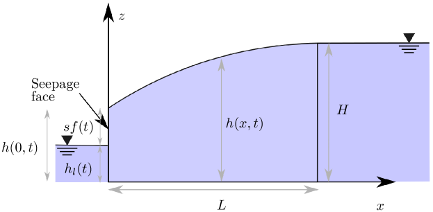
Figure 1: Schematic of the Di Nucci model showing constant head $H$ at $x=L$, transient seepage face height $sf(t)$ at $x=0$, transient lake height $h_{l}(t)$, and transient free surface height $h(x,t)$. The heights are calculated from the the impermeable base at $z=0$. The domain extends from $x=0$ to $x=L$. Also, the seepage face height $sf(t)=h(0,t)-h_{l}(t)$. The same figure can be used for the Dupuit-Boussinesq model by changing two underlying assumptions. First, the Dupuit-Boussinesq model assumes the seepage face height $sf(t)$ to be zero. Second, the far-field head $h(x,L)$ is not specified.

This model couples a Boussinesq-type equation with Darcy’s law and solves a one-dimensional PDE resulting from the two-dimensional unsteady free surface flow in a homogeneous, isotropic medium [Di Nucci (2018)], as shown in schematic diagram 1. The vertical flow is included by considering a higher-order, implicit term in the flux formulation. This term is given in Equation (5), as well as the first-order term associated with Darcy’s law. A unique solution is possible using a boundary condition with time dependent flux at the seepage face, $x=0$, (7) and a constant hydraulic head level at the upstream boundary, $x=L$ (8). Moreover, the seepage face development is accounted for by a mass and momentum balance as well as Cauchy’s integral relation theorem for potential and stream function relationships [Bear (1972), Di Nucci (2018)]. The resulting governing equations take the form:

$$\frac{q}{K} = -\frac{\partial}{\partial x}\left[\frac{h^{2}}{2}-\frac{1}{K}\frac{\partial}{\partial x}\left(\frac{q}{h}\right)\frac{h^{3}}{3}\right]$$ (5)

$$\frac{1}{K}\frac{\partial q}{\partial x} = -\frac{\phi}{K}\frac{\partial h}{\partial t},\qquad t\in[0,\infty),\quad x\in[0,L]$$ (6)

subject to boundary conditions:

$$\frac{q}{K}(0,t) =g(t)$$ (7)

$$h(L,t) =H=\textrm{constant}$$ (8)

where $q(x,t)=Q(x,t)/w$ is the discharge per unit width (m³/m.s). $g(t)$ is considered a function of time to reproduce the boundary condition of the 2D problem, which can be considered as

$$\frac{q}{K}(0,t) =\frac{H^{2}-h_{l}^{2}(\infty)}{2L}$$ (9)

for a steady-state lake level of $h_{l}(\infty)$. The integral relation arising from Cauchy theorem is

$$\frac{1}{2}h_{l}^{2}(t)=\frac{1}{2}H^{2}-\int_{0}^{L}\frac{1}{K}q(x,t)\mathrm{d}x$$ (10)

where $h_{l}(t)$ is the time varying height of lake, not considered in Dupuit-Boussinesq approximation. The transient seepage face height $sf(t)$ (in m) can then be calculated using

$$sf(t)=h(0,t)-h_{l}(t)=h(0,t)-\sqrt{H^{2}-2\int_{0}^{L}\frac{1}{K}q(x,t)\mathrm{d}x}$$ (11)

For steady-state, Equation (5) and (10) take the form

$$\frac{q}{K} =-\frac{\mathrm{d}}{\mathrm{d}x}\left(\frac{h^{2}}{2}+\frac{q}{K}\frac{\mathrm{d}h}{\mathrm{d}x}\frac{h}{3}\right)$$ (12)

$$\frac{q}{K} =\frac{H^{2}-h_{l}^{2}(\infty)}{2L}$$ (13)

Also, $q(x,\infty)=Q/w$ becomes a constant in both space and time, stemming from Equation (6). For the boundary conditions,

$$\frac{\mathrm{d}h}{\mathrm{d}x}(L,\infty)=0\quad\textrm{and}\quad h(L,\infty)=H,$$ (14)

the analytical result for free-surface height $h(x,\infty)$ is

$$h(x,\infty) =\sqrt{H^{2}-\frac{2Q(L-x)}{Kw}+\frac{2}{3}\frac{Q^{2}}{K^{2}w^{2}}\left[1-\exp\left(-\frac{3Kw(L-x)}{Q}\right)\right]}$$ (15)

Coupling (15) with (13) gives the steady-state seepage face height as

$$sf(\infty) =h(0,\infty)-h_{l}(\infty)=\frac{2Q^{2}}{3K^{2}w^{2}}\frac{\left(1-\exp\left(-\frac{3KwL}{Q}\right)\right)}{h(0,\infty)+h_{l}(\infty)}.$$ (16)

As such the Di Nucci model determines the unknown steady height of the groundwater table, $h(0,\infty)$, at the seepage face.

3 Physics informed neural networks

3.1 Deep neural networks for approximating functions

Deep neural networks have been extensively studied for the purpose of approximating arbitrary functions [Hornik . (1989)]. We refer to [Goodfellow . (2016)] for a full exposition of neural networks and its training, and [Lu . (2021)] for its application to the context of approximating solutions to PDEs. Here, we present the formulation for a standard, feed-forward neural network, such as that described in [Lu . (2021)]. A feed-forward neural network defines the mapping from an input $\mathbb{R}^{\text{in}}$ to output space $\mathbb{R}^{\text{out}}$ based on successive, non-linear transformations through layers of neurons. We refer to the first layer as the input layer, the final layer as the output layer, and additional layers as as hidden layers. Activation values are passed from one layer to the next via an activation function composed with a linear transformation. The neural network mapping, $u_{NN}(x)$, given an input vector, $x\in\mathbb{R}^{\text{in}}$, can be mathematically represented as

$$u_{NN}(x;\theta):=(v_{N-1}\circ v_{N-2}\circ...\circ v_{1})(x),$$ (17)

where $\circ$ denotes the composition of two functions (i.e. $(v_{2}\circ v_{1})(x)=v_{2}(v_{1}(x))$ and $v_{i}$ maps the $i^{\text{th}}$ layer to its following layer through

$$v_{i}(x) =\sigma_{i}(W_{i}x+b_{i})\text{ for }i=1,2,...,N.$$ (18)

In this representation, transformations between the layers are parameterized by weights $W_{i}\in\mathbb{R}^{n_{i}\times n_{i-1}}$ and biases $b\in\mathbb{R}^{n_{i}}$, collectively referred to as $\theta=\{W_{i},b_{i}\}_{i=1}^{N-1}$. Here, $N$ is the total number of layers and $n_{i}$ is the width of the $i^{\text{th}}$ layer. The function $\sigma_{i}(\cdot)$ is the activation function for the $i^{\text{th}}$ layer, which is typically a nonlinear function applied element-wise to its input vector. The possible choices for the activation function are numerous and include common implementations such as the sigmoid, ReLu and softplus functions [Goodfellow . (2016), Lu . (2021)]. The activation function, for the output layer, can be chosen based on the desired output of the neural network. Derivatives of the neural network output with respect to the inputs, weights, and biases, can be obtained using automatic differentiation.

Given a training dataset $\mathcal{S}_{t}=\{(x_{i},u_{i})\}_{i=1}^{N_{t}}$ consisting of $N_{t}$ inputs $x_{i}$ and outputs $u_{i}$, it is possible to train the neural network by minimizing a loss function. For example, using the mean squared error MSE between the neural network outputs and the training data, we can write

$$\theta^{*}=\mathrm{arg}\min_{\theta}\frac{1}{N_{t}}\sum_{i=1}^{N_{t}}(u(x_{i};\theta)-u_{i})^{2}$$ (19)

where $\theta^{*}$ represents the optimal weights and biases. The optimization problem within training the neural network is frequently solved using gradient based optimization algorithms such as stochastic gradient descent [Bottou (2010)], ADAM [Kingma  Ba (2014)], and limited-memory BFGS (L-BFGS) [Liu  Nocedal (1989)].

To avoid overfitting, additional regularization terms may be included in the loss function such as $l_{1}$ or $l_{2}$ norms of the weights and biases [Goodfellow . (2016)]. For deep neural networks with a large number of neurons, a process known as dropout, whereby random weights and biases are omitted during training, can also be employed during training as a form of regularization [Srivastava . (2014)].

3.2 PINNs for solving forward and inverse problems

3.2.1 Learning forward solutions

Physics informed neural networks [Raissi . (2019)] aim to enforce physics based constraints on the neural network to improve the effectiveness of the technique when applied to data arising from physical systems [Tartakovsky . (2020)]. Supposing a physical system has state $u(x,t)$ which is governed by a nonlinear PDE of the form

$$u_{t}+\mathcal{N}(u;\lambda)=0,$$ (20)

where $\mathcal{N}$ is a nonlinear differential operator and $\lambda$ consist of parameters defining the PDE. Within the PINNs framework, the state $u(x,t)$ is approximated by a feedforward neural network $u_{NN}(x,t)$, as defined in (17). Information given by the PDE is incorporated into the training of the neural network by defining the loss function as

$$\mathcal{L}(\mathcal{S}_{t},\mathcal{S}_{c},\theta) =\text{MSE}_{u}+\alpha\text{MSE}_{f},$$ (21)

where

$$\text{Data misfit, }\text{MSE}_{u} =\frac{1}{N_{t}}\sum_{i=1}^{N_{t}}(u_{NN}(x_{i},t_{i})-u_{i})^{2},$$ (22)

$$\text{PDE misfit, }\text{MSE}_{f} =\frac{1}{N_{c}}\sum_{i=1}^{N_{c}}|f(x_{i},t_{i};\lambda)|^{2}.$$ (23)

Here, MSE is the mean-squared error loss term and is referred to as the misfit term in this paper. Moreover, $f(x,t):=u_{t}(x,t)+\mathcal{N}(u(x,t);\lambda)$ is the PDE residual, $N_{t}$ is the number of data points in the training set $\mathcal{S}_{t}=\{(x_{i},t_{i},u_{i})\}_{i=1}^{N_{t}}$, $N_{c}$ is the number of collocation points of the form $\mathcal{S}_{c}=\{(x_{j},t_{j})\}_{j=1}^{N_{c}}$, and $\alpha$ is the PDE regularization parameter. The data misfit term, $\text{MSE}_{u}$, is evaluated on the training data points where the state is known, and $\text{MSE}_{f}$ is evaluated on $N_{c}$ collocation points $(x_{i},t_{i})\in\mathcal{S}_{c}$ where the state is not necessarily known. The $\text{MSE}_{f}$ adds physics information to the neural network by encouraging the satisfaction of the governing PDE on the collocation points. The parameter $\alpha$ can be chosen to balance the relative effects of data and PDE in training the neural network. Once trained, the optimal weights and biases are determined as $\theta^{*}$

$$\theta^{*}=\mathrm{arg}\min_{\theta}\mathcal{L}(\mathcal{S}_{t},\mathcal{S}_{c},\theta).$$ (24)

and the resulting neural network $u_{NN}$ is used to predict the state at desired points $(x,t)$.

This formulation of PINNs can be used as a solver for the PDE by supplying initial and boundary conditions as training data and using points on the interior of the domain as collocation points for evaluating the PDE misfit [Raissi . (2019)]. The neural network is then trained to fit the initial and boundary data while satisfying the PDE.

3.2.2 Learning parametrized forward-solutions

We also consider a parametrization of the problem involving an additional input variable, $q$. To do so, we construct the neural network approximation, $u_{NN}(x,t,q)$, with the additional input variable, $q$. We train the neural network using training data $\mathcal{S}_{t}=\{(x_{i},t_{i},q_{i},u_{i})\}_{i=1}^{N_{t}}$ corresponding to different values of the input variable. We adopt the same loss function as in (21) with

$$\text{Data misfit, }\text{MSE}_{u} =\frac{1}{N_{t}}\sum_{i=1}^{N_{t}}(u_{NN}(x_{i},t_{i},q_{i})-u_{i})^{2},$$ (25)

$$\text{PDE misfit, }\text{MSE}_{f} =\frac{1}{N_{t}}\sum_{i=1}^{N_{t}}|f(x_{i},t_{i},q_{i};\lambda)|^{2},$$ (26)

in which we use the training data points to evaluate both the data and PDE misfits. Again, we can optimize for the weights and biases to obtain our neural network approximation.

In this approach, the neural network is essentially trained on data with the PDE as a form of regularization. The resulting neural network predictions represent a fitting of training data that is also informed by the physics associated with the PDE and scaled with the weighing parameter $\alpha$. Therefore, the PDE used does not need to capture the entire physics of the system. In particular, we can adopt this approach when initial or boundary conditions are not specified because the the PDE is only used as regularization and does not need to be solved in training.

3.2.3 Inverting for model parameters

When model parameters $\lambda$ are unknown, they can be inverted for in training by defining them as additional optimization variables in addition to weights and biases $\theta$. The optimization problem then takes the form

$$(\theta^{*},\lambda^{*})=\mathrm{arg}\min_{\theta,\lambda}\mathcal{L}(\mathcal{S}_{t},\mathcal{S}_{c},\theta,\lambda).$$ (27)

It must be noted that in either case (24 or 27), the PDE does not need to be exactly satisfied by the trained neural network. Instead, the PDE misfit is only minimized to the extent achievable by the training process. Therefore, the recovered parameter values have a meaningful physical interpretation only when the PDE is well satisfied by the neural network. Otherwise, the recovered parameters serve only to improve predictions made by the neural network.

4 PINNs for examining steady unconfined groundwater flows

We apply PINNs in the context of steady groundwater seepage in homogenous porous media. Physics information is incorporated into the training of the PINNs through PDE models of quasi-1D seepage flow. In particular, we consider both the Dupuit-Boussinesq equation and Di Nucci’s equation as potential models.

4.1 PDE models

Under steady-state conditions, the Dupuit approximation is given by

$$q+Kh\frac{\mathrm{d}h}{\mathrm{d}x}=0\quad x\in(0,L)$$ (28)

and Di Nucci’s model takes the following form (12)

$$q+Kh\frac{\mathrm{d}h}{\mathrm{d}x}+\frac{q}{3}\frac{\mathrm{d}}{\mathrm{d}x}\left(h\frac{\mathrm{d}{h}}{\mathrm{d}x}\right)=0.\quad x\in(0,L)$$ (29)

In both equations, $q$, the flow rate per unit width, is constant in space, and parameterizes the flow profile $h(x)$. For the purpose of training, we non-dimensionalize the two equations by this non-zero constant such that the source term is of $\mathcal{O}(1)$. In this case, the residual of the Dupuit equation can be re-written as

$$f_{\text{Dupuit}}(h,q;K):=1+\frac{K}{q}h\frac{\mathrm{d}h}{\mathrm{d}x}=0\quad x\in(0,L)$$ (30)

and the residual of the Di Nucci equation becomes

$$f_{\text{DiNucci}}(h,q;K):=1+\frac{K}{q}h\frac{\mathrm{d}h}{\mathrm{d}x}+\frac{1}{3}\frac{\mathrm{d}}{\mathrm{d}x}\left(h\frac{\mathrm{d}{h}}{\mathrm{d}x}\right)=0\quad x\in(0,L).$$ (31)

Here flow rate per unit width, $q$, is constant throughout the domain due to the absence of recharge.

4.2 Learning flow-parameterized solutions to seepage equations

To approximate phreatic surface profiles, parameterized by the flow rate per unit width $q$, we use both the Dupuit and Di Nucci approximations to seepage flow. To do so, we construct a neural network, $h_{NN}$, defined as a function of two input variables. These are the longitudinal position, $x$, and the flow rate per unit width, $q$. We seek a neural network approximation, $h_{NN}(x,q)$, for the flow profile given training data of the free surface height, $h_{i}$, that is labeled by the inputs $(x_{i},q_{i})$. This formulation is the steady-state and therefore, the time component can be neglected.

In addition to the flow rate, the PDEs considered are parameterized by the hydraulic conductivity, $K$, which is treated as a constant throughout the domain. Thus, in the steady-state case, we have PDEs of the form

$$f(h(x),q;K)=0,\quad x\in\Omega\text{,}$$ (32)

using either $f=f_{\text{Dupuit}}$ or $f=f_{\text{DiNucci}}$. This allows us to define the training loss as

$$\mathcal{L}(\mathcal{S}_{t},\theta,K)=\frac{1}{N_{t}} \sum_{i=1}^{N_{t}}(h_{NN}(x_{i},q_{i};\theta)-h_{i})^{2}+\frac{\alpha}{N_{t}}\sum_{i=1}^{N_{t}}|f(h_{NN}(x_{i},q_{i}),q_{i};K)|^{2}.$$ (33)

given training data $\mathcal{S}_{t}=\{(x_{i},q_{i},h_{i})\}_{i=1}^{N_{t}}$. Note that we evaluate the PDE misfit on the same points as the training data, as in Equations (25) and (26). As previously discussed, $\alpha$ values can be tuned to balance the relative effects of data versus the PDE.

Typically, boundary conditions are also required to solve for the complete flow profile using the PDEs. However, it is practically difficult to determine appropriate boundary conditions for both the Dupuit-Boussinesq and Di Nucci equations. In the presence of a seepage face, the downstream piezometric head is not zero and is instead unknown a priori. On the other hand, our experimental design only fixes the steady-state flow rate and not the upstream hydraulic head level. As a result, we cannot specify the additional Dirichlet boundary condition required to solve the PDE. It is therefore crucial that the PINNs formulation does not impose any boundary conditions. Instead, the PDE is used as regularization for the flow profile on the interior of the domain and the data helps to inform the neural network about the boundary information.

When accurate estimates for hydraulic conductivity, $K$, are not available, we can invert for the value of $K$ during training based on the training data. To do so, we consider $K$ as a variable that may be optimized in training, which is updated based on the loss function (33). Due to the uncertainties associated with the experimentally measured $K$, inverting for $K$ in training potentially produces a model that better fits the training data.

4.3 PINNs implementation

The investigation is performed using a fully connected feed-forward neural network with $(x,q)$ as input layer and $h_{NN}$ as the output layer. Figure 2 shows the architecture diagrams of the PINNs based on Di Nucci model. The neural network has 5 hidden layers, each layer being 20 neurons wide. The hyperbolic-tangent activation function is used for all hidden layers, while a softplus activation function is used for the output layer such that $h_{NN}(x)>0$. The output of the neural network $h_{NN}$ is automatically differentiated, which is used to form the PDE misfit term. The PDE misfit, along with data misfit, forms the loss function (33) which is then minimized to predict the optimal weights and biases $\theta^{*}$ (24), and model parameters $\lambda^{*}$ (hydraulic conductivity $K$) (27).

We employ a combination of the ADAM and L-BFGS optimization algorithms to train the neural networks. In all training cases, we perform 50,000 ADAM iterations followed by L-BFGS until convergence to a tolerance of $\epsilon_{g}=10^{-8}$ on the norm of the gradient of the loss function.

Figure 2: Neural network architecture diagrams of PINNs for investigating steady-state groundwater flows using Di Nucci model.

4.4 Selection of a regularization parameter for the PDE misfit term

A scaling analysis of the competing terms in the loss function aids in selecting the PDE misfit regularization parameter $\alpha$. Considering a trivial neural network $h_{NN}=0$, we observe that the data misfit term is

$$\mathrm{\text{MSE}}_{h}=\frac{1}{N_{t}}\sum_{i=1}^{N_{t}}(h_{i}-h_{NN}(x_{i}))^{2}\sim\mathcal{O}(\bar{h}^{2}),$$

where $\bar{h}$ is some characteristic value of free-surface height from the training data. On the other hand, the PDE misfit term is

$$\mathrm{\text{MSE}}_{f}=\frac{1}{N_{t}}\sum_{i=1}^{N_{t}}f_{NN}(x_{i})^{2}\sim\mathcal{O}(1),$$

due to our choice of normalization for the PDE. Thus, with a choice of $\bar{\alpha}=\mathcal{O}(\bar{h}^{2})$, we expect the significance of the data misfit to be comparable to that of the PDE misfit. In this work, we take

$$\bar{\alpha}:=\frac{1}{N_{t}}\sum_{i=1}^{N_{t}}|h_{i}|^{2}$$ (34)

as the reference value of the regularization parameter.

5 Data generation

Synthetic data is generated using the analytical solutions of the two PDEs; (4) for the Dupuit-Boussinesq and (15) for the Di Nucci models respectively. The analytical results $h(x)$ at selected values of $(x_{i},q_{i})$ are then corrupted by Gaussian white noise with standard deviation that is $1\%$ of the maximum $h(x)$ in the dataset. Synthetic data is used to test the performance of the neural networks as both the model and its parameters are known. We also perform our analysis on experimental data of steady groundwater flow, obtained using the experimental design shown in figure 3. The setup consists of an acrylic cell of length 167 cm, height 45 cm and width 2.54 cm (in third dimension) which contains a porous region filled with beads of diameter 1 or 2 mm. Dyed water is pumped from right boundary $x=L$ at a specified flow rate which subsequently drains from the seepage face on the left boundary $x=0$ with zero head at the gravity well, i.e., $h_{l}=0$. A camera, placed orthogonally in front, takes pictures which are then processed using a Matlab code to digitize and extract the free surface profiles.

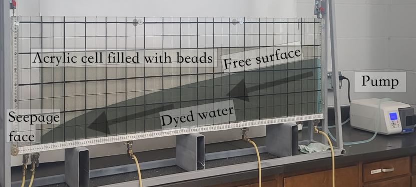
Figure 3: A picture of the experimental setup.

It is common practice in neural network training to normalize the dataset such the different input variables are comparable in size [Priddy  Keller (2005)]. In our application, input values for $x$ and $q$ typically differ by several orders of magnitude. Therefore we scale the training data by the order of magnitudes of their maximum values, which for the experimental data are $1$ $(\mathrm{m})$ and $10^{-4}$ $(\mathrm{m}^{2}/\mathrm{s})$ for the $x$ and $q$ variables respectively.

6 Steady-state results using synthetic data

6.1 Learning parameterized solutions from synthetic data

Synthetic data $(x_{i},q_{i},h_{i})$ is generated from 8 linearly spaced flow values of $q=Q/w\in[10^{-4},10^{-3}]$ m²/s and 50 equidistant points of $x\in[0,1]$ m with $K=0.01$ m/s. These values resemble those used in the experimental data.

6.1.1 Regularization

We first investigate the effects of the regularization parameter $\alpha$. PINNs is trained by increasing values of $\alpha$ from $\alpha=0$ up to $\alpha=10^{4}\overline{\alpha}$. Here $\alpha=0$ corresponds to a plain neural network which does not incorporate any physics information. For the training values of $q$, we plot the noisy, free-surface data along with the predictions of the neural networks trained using each value of $\alpha$. These are shown in Figures 4 and 6 for the Dupuit and Di Nucci equations respectively.

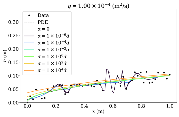
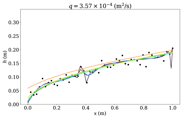
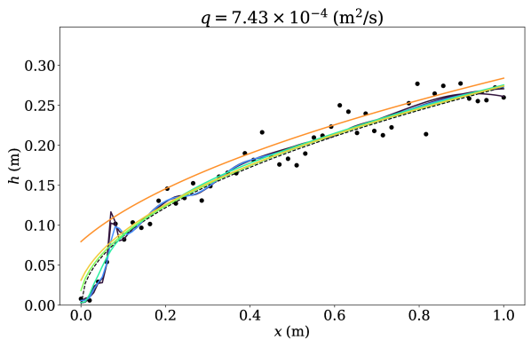
Figure 4: Neural network predictions of free surface profiles with varying $\alpha$ ($\overline{\alpha}={h}^{2}$), using the Dupuit equation as the regularizing PDE. The plots show the effect of changing the specific discharge $q=Q/w=10^{-4}-10^{-3}$ m${}^{3}/$m.s (shown in titles) and PDE regularization parameter $\alpha=0-10^{4}\overline{\alpha}$. Data and PDE refer to the noisy and noiseless data, respectively.

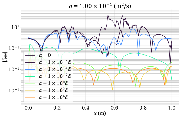
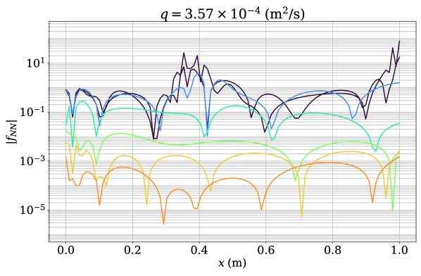
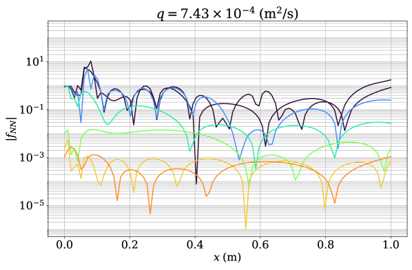
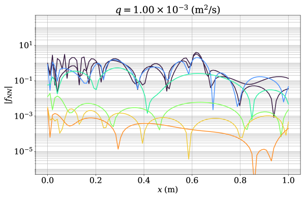
Figure 5: PDE residuals inside the domain corresponding to free surface profiles shown in Figure 4 for Dupuit model based PINNs predictions.

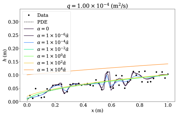
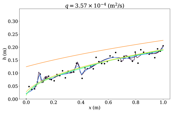
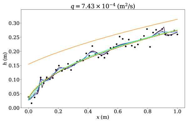
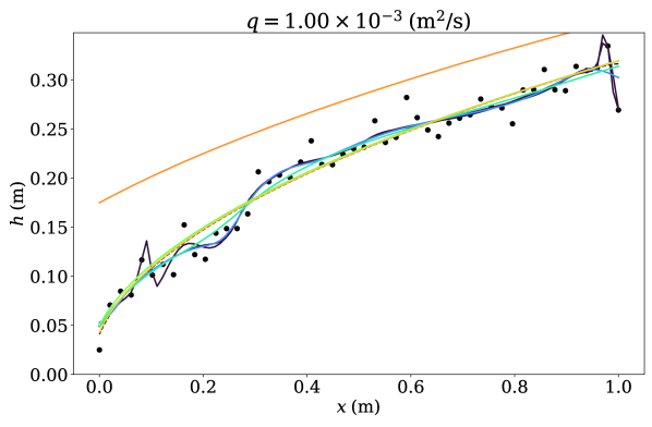
Figure 6: Neural network predictions with varying $\alpha$ and specific discharge $q$, using the Di Nucci equation as the regularizing PDE.

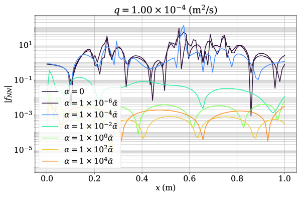
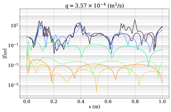
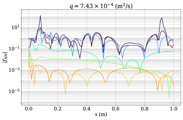
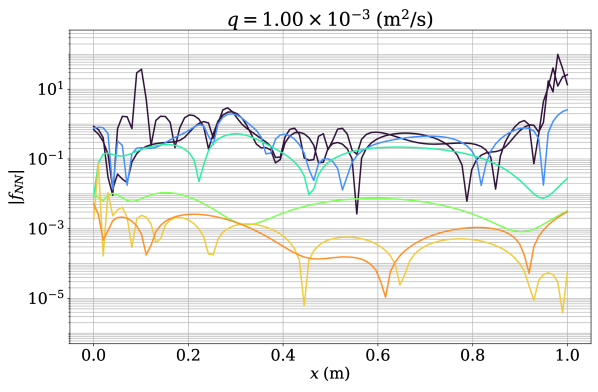
Figure 7: The PDE residuals inside the domain corresponding to free surface profile predictions, shown in Figure 6, using PINNs regularized by Di Nucci equation.

In general, we observe extreme overfitting for small values of $\alpha$ due to the lack of regularization. The overfitting is reduced by increasing $\alpha$, as the PDE is more strongly respected relative to the training data. This happens due to the introduction of the physics information to the neural network from the PDE misfit term in objective function. Increasing $\alpha$ increases the accuracy of the predictions with respect to the PDE results. In general, PINNs give good and robust predictions however, a typical NN ($\alpha=0$) does not. For $\alpha=\{\overline{\alpha},100\overline{\alpha}\}$, the predictions are very close. But when $\alpha=10^{4}\overline{\alpha}$ the PDE misfit overshadows the data misfit and therefore, the NN predictions disregard the data, leading to significant deviation from the data. So, it is necessary to find the optimal value of the regularization parameter.

This effect is illustrated further in the plots of PDE residuals inside the domain corresponding to free surface profiles, shown in Figures 5 and 7 for Dupuit and Di Nucci models respectively. It is again evident that increasing $\alpha$ decreases the PDE residual as the penalty in the objective function augments. Close to the seepage face ($x\to 0$), the PDE residual typically increases as the free surface height changes rapidly and the data points to capture the change are relatively small. The case of no PDE misfit $\alpha=0$ generally has the highest residual. The residual is less than $10^{-1}$ at most points in the domain for $\alpha\geq\overline{\alpha}$.

This effect of PDE misfit reduction with $\alpha$ can be summarized by an L-curve analysis, in which we plot the data misfit against the PDE misfit on the log-scale, as predicted by each neural network. In particular, we define the cumulative data misfit as a sum of squared errors (SSE),

$$\mathrm{SSE}_{h}=\sum_{i=1}^{N_{t}}(h_{NN}(x_{i},q_{i})-h_{i})^{2},$$ (35)

and the cumulative PDE misfit as

$$\mathrm{SSE}_{f}=\sum_{i=1}^{N_{t}}|\mathcal{N}(h_{NN}(x_{i}),q_{i};K)|^{2}.$$ (36)

The L-curves are shown in Figures 8 and 9 for the Dupuit and Di Nucci equations respectively. The resulting curve demonstrates that as $\alpha$ increases, the data misfit increases while the PDE misfit decreases. The L-curve analysis shows the optimal $\alpha$ in the range $\overline{\alpha}$ to $10\overline{\alpha}$. This is consistent with order of magnitude argument provided in section 4.4 to estimate the optimal $\alpha$. There is a sharp increase in the data misfit for $\alpha>10^{3}\overline{\alpha}$ as the neural network disregards the data misfit and tries to minimize the PDE misfit only. This suggests that $\alpha$ values in the optimal range [$\overline{\alpha},10\overline{\alpha}$] represent an appropriate balance between fitting the data and satisfying the PDE.

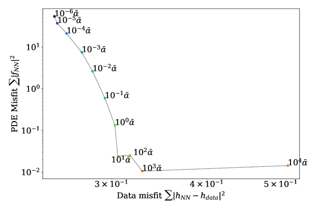
Figure 8: L-curve analysis using the Dupuit equation as the regularizing PDE corresponding to tests shown in Figures 4 and 5.

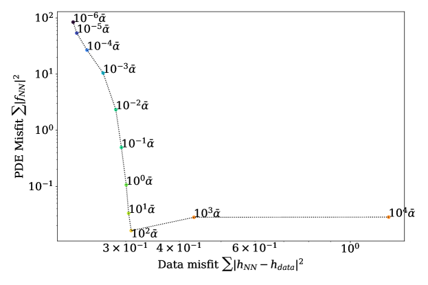
Figure 9: L-curve analysis using the Di Nucci equation as the regularizing PDE corresponding to tests shown in Figures 6 and 7.

6.2 Inversion for hydraulic conductivity

From the synthetic data, we also invert for the hydraulic conductivity, $K$. This is done by including $K$ as an optimization variable during the training of the neural network. We consider three different regularization parameter values, ${\alpha}=\{\overline{\alpha},5\overline{\alpha},10\overline{\alpha}\}$, based on the scaling described in the previous section. The trained neural network predictions are shown in Figure 10 for the Dupuit equation and Figure 12 for the Di Nucci model. Furthermore, the inverted values of $K$ are summarized in Table 1. It can be observed that all regularization parameters ${\alpha}=\{\overline{\alpha},5\overline{\alpha},10\overline{\alpha}\}$ fit the synthetic data very well and cannot be visually distinguished from each other.

Moreover, their corresponding PDE misfits are small ($<2\times 10^{-2}$) throughout the domain, as shown in Figures 11 and 13 for the Dupuit and Di Nucci models, respectively. Increasing $q$ makes the free surface profile steeper at the seepage face, which causes more resolution errors leading to relatively higher PDE residual near the seepage face. But in general, the inversion yields accurate values of $K$ for both the Di Nucci and Dupuit equations. This gives us confidence that including $K$ as an optimization variable allows us to train PINNs that produce accurate predictions while recovering accurate estimates for the hydraulic conductivity $K$ in the process.

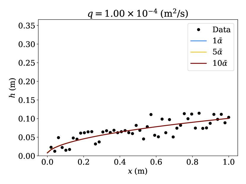
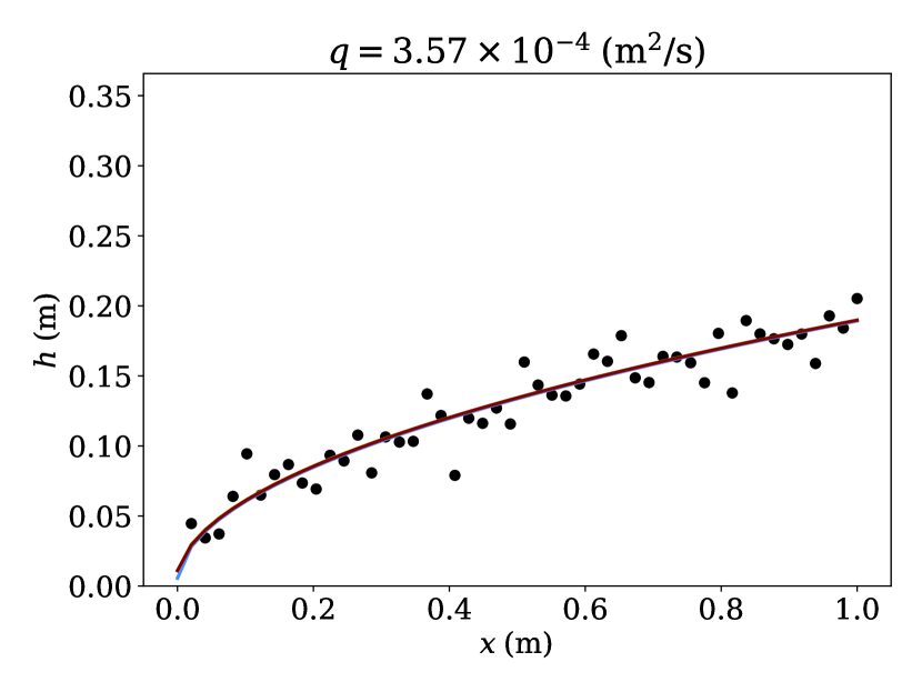
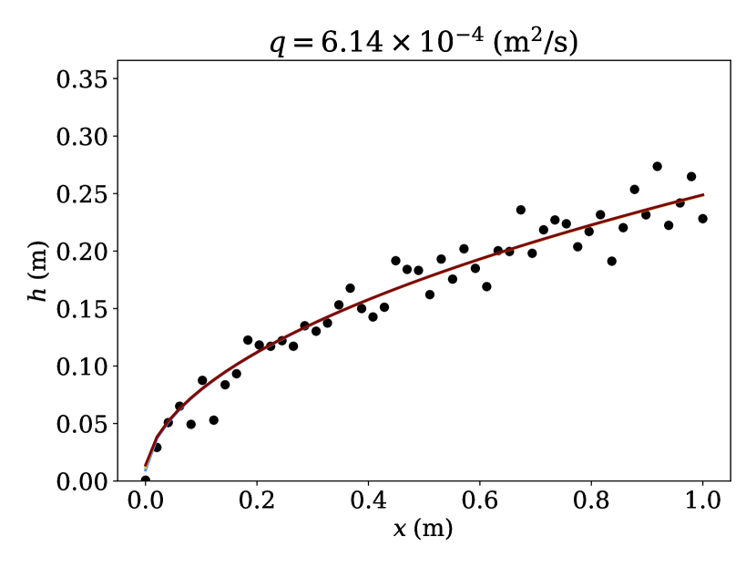
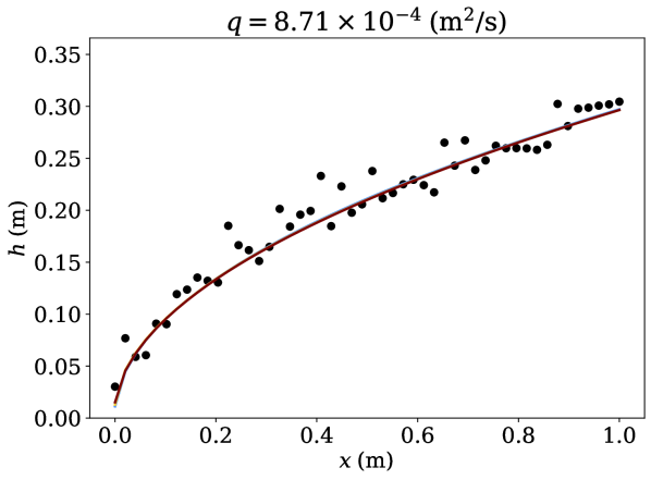
Figure 10: Training data and neural network predictions for free surface height while inverting for $K$, using the Dupuit equation as the regularizing PDE.

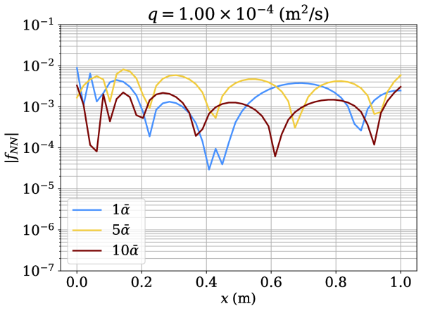
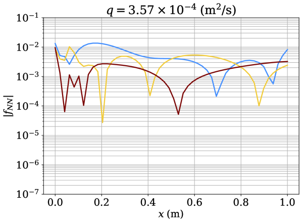
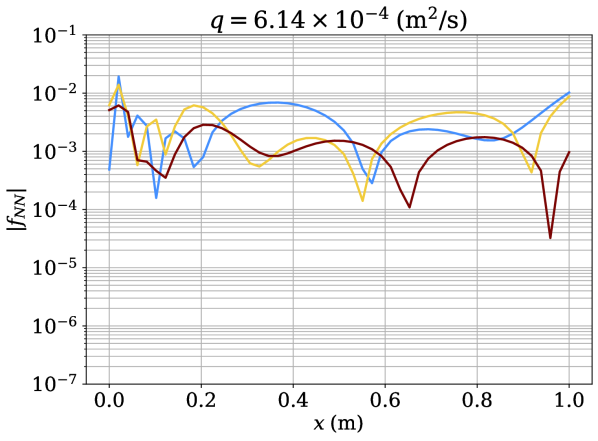
Figure 11: The PDE misfit terms inside the domain while inverting for $K$, corresponding to Figure 10, using the Dupuit equation as the regularizing PDE.

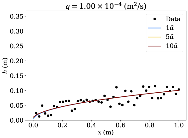
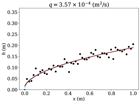
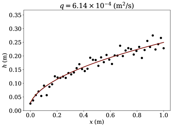
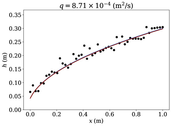
Figure 12: Training data and neural network predictions for free surface height while inverting for $K$, using the Di Nucci equation as the regularizing PDE.

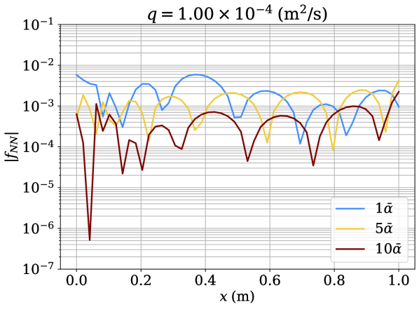
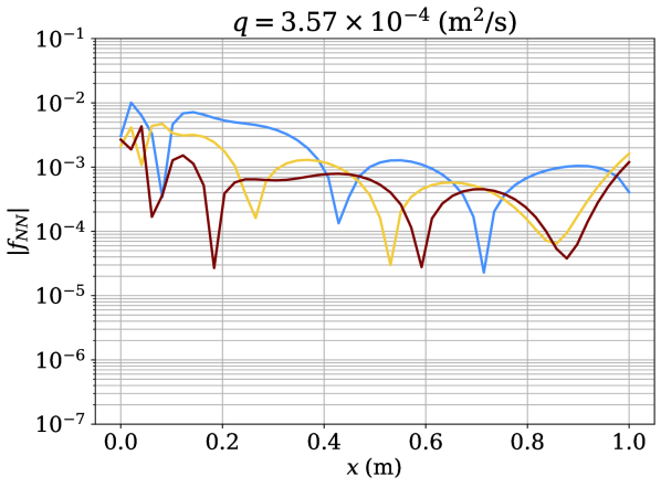
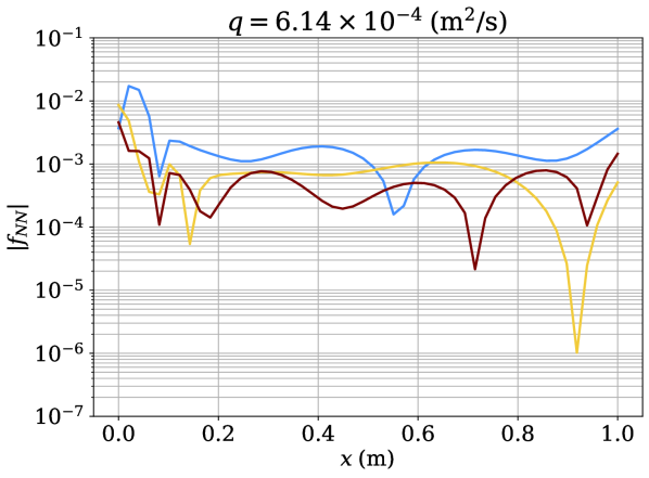
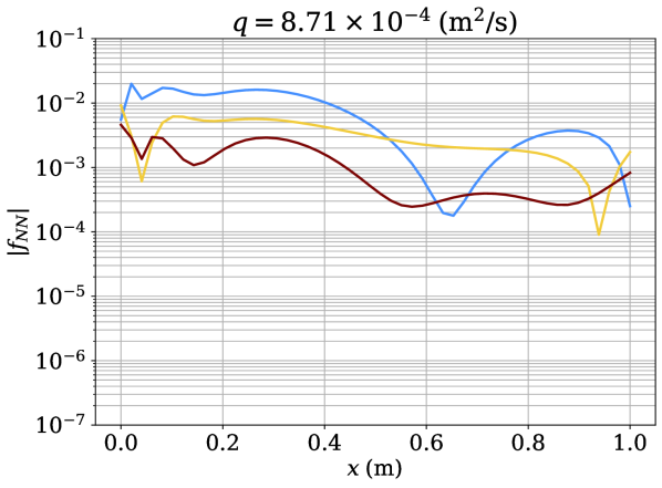
Figure 13: PDE residual for Di Nucci model based PINNs predictions corresponding to Figure 12 for different regularization parameters.

	Hydraulic conductivity $K$	Error
Truth	0.020000	-
Di Nucci equation
$\alpha=\bar{\alpha}$	0.019945	0.268%
$\alpha=5\bar{\alpha}$	0.020028	0.140%
$\alpha=10\bar{\alpha}$	0.019990	0.064%
Dupuit Equation
$\alpha=\bar{\alpha}$	0.019910	0.452%
$\alpha=5\bar{\alpha}$	0.019958	0.209%
$\alpha=10\bar{\alpha}$	0.019913	0.434%

Table 1: Recovered $K$ values from synthetic training data generated from PINNs with Di Nucci equation (top) and Dupuit equation (bottom).

6.3 Comparison of terms in the Di Nucci equation

In addition to prediction of flow profiles and inversion of $K$, we demonstrate the use of PINNs for determining the relative contributions of terms in a PDE from given flow data. In A, a non-dimensional parameter $\Pi=2q/KL$ is derived by scaling Di Nucci equation (5) which indicates the ratio of vertical to horizontal flow terms. We expect that for large $\Pi$ values, the higher order term corresponding to vertical flow effects play larger roles in the PDE residual. For testing, we perform a numerical experiment in which the Di Nucci equation is used as the model for generating individual sets of training data for $K=[0.02,0.004,0.002,0.0002]$ m/s, corresponding to $\Pi=[0.1,0.5,1,10]$. Physics based neural networks are then trained separately for each set of training data, inverting for the $K$ value during the process. After training, we leverage the automatic differential capabilities to compute the terms in the Di Nucci equation. This allows us to identify the significance of the Di Nucci terms for different flow scenarios, which then lets us comment on the appropriateness of the Dupuit approximation compared to the Di Nucci model for different sets of flow data coming from the experiments.

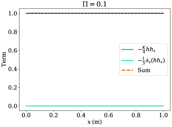
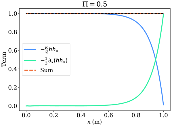
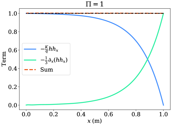
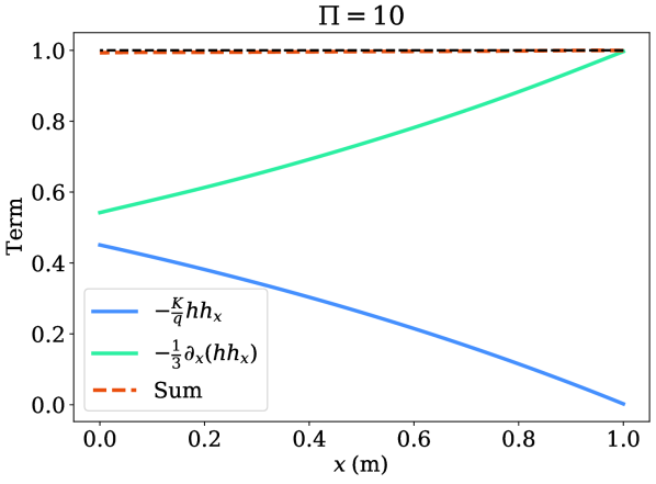
Figure 14: Variation of PDE terms of Di Nucci model across the domain for different $\Pi$ values.

We plot the PDE terms computed by the trained PINNs for each training set in Figure 14. As expected, it can be observed that for larger values of $\Pi$, the higher order term $\partial_{x}(hh_{x})/3$ is the dominant PDE term across the domain, while for $\Pi=0.1$, this term is negligible. Increasing $\Pi$ corresponds to the rise in the specific discharge over the horizontal seepage, leading to higher order vertical flow effects. This suggest that the Dupuit approximation $q=-Khh_{x}$ is valid for $\Pi\leq 0.1$ but not for $\Pi>0.1$. Increasing $\Pi$ to $0.5$ shows a considerable rise in the higher order vertical flow term, especially close to the far field boundary due to the far field boundary conditions (14) assumed in derivation of the Di Nucci’s steady-state analytical result. The term drops at the seepage boundary. When $\Pi$ is large, here 10, the trends become almost linear, the higher order term tends to unity across the whole domain.

7 Steady-state results using experimental data

We next trained neural networks on the experimental data, considering data from 1 mm and 2 mm beads separately. In the 1 mm data set, we have flow profiles for 10 different flow rates while for the 2 mm data set we have 12 different flow rates. For simplicity, the height of the lake, $h_{l}$, is set to zero for all experiments, but this model can be easily applied to non-zero lake level. For each bead size, we take flow profiles from half of the flow rates as training data, and use the remaining datasets as test sets. We train PINNs using the Di Nucci and Dupuit equations as regularization with $\alpha=\bar{h}^{2}$, and consider both having fixed $K$ taken from theoretical estimates, as well as freeing up $K$ for inversion during training. We also train plain neural networks without physics informed regularization as a reference.

7.1 Flow data prediction

The predictions for the trained neural networks, with and without physics informed regularization, are shown in Figure 15 and 17 for 1 mm and 2 mm beads respectively. The plots show the best and the worst cases among all the cases considered. The plots for all other test cases are provided in the supplementary file. Although a plain neural network performs well on the training data, it performs poorly on test data when compared with PINNs, as it considers the data misfit only. The PINNs predictions for fixed $K$, pre-calculated using Cozeny-Karman relation for permeability [Bear (1972)], overpredicts the seepage face height but is very close to the data. Both Dupuit and Di Nucci based PINNs give predictions very close to each other. The plain neural network performs fairly well but has oscillations due to overfitting the noise, but the PINNs predictions do not have these oscillations. The PINNs predictions for fixed $K$ overpredicts the seepage face height for 1 mm beads but underpredicts the seepage face height for 2 mm bead data.

The corresponding PDE residuals across the domain are shown in Figures 16 and 18 for Dupuit and Di Nucci cases. It can be observed that the PDE residual for the plain neural network is the highest, whereas for the case of fixed $K$ values is less than $0.1$ almost everywhere.

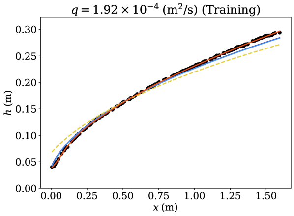
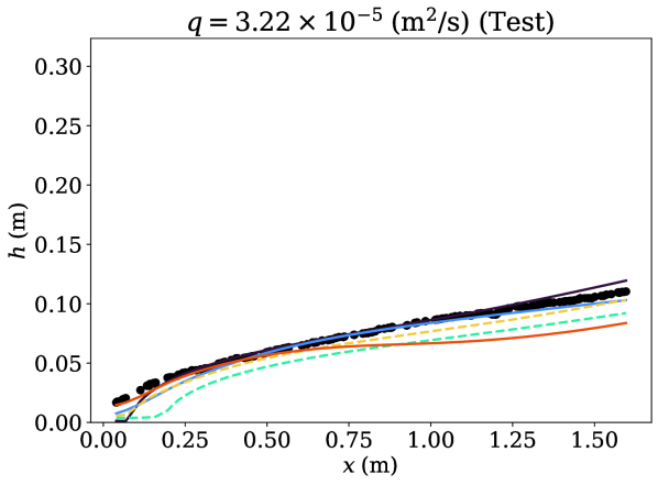
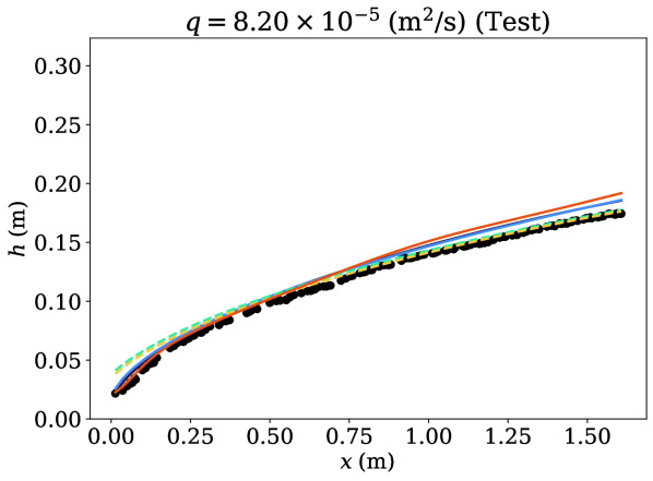
Figure 15: Neural network predictions of free surface profiles for the experimental data using 1 mm beads.

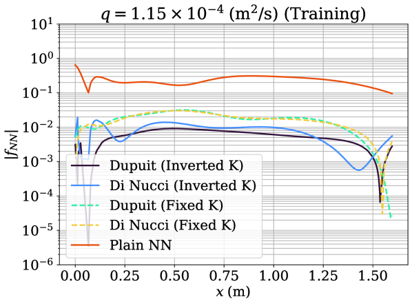
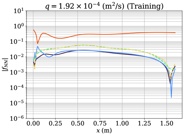
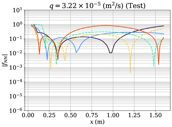
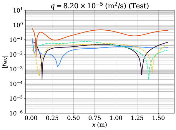
Figure 16: The PDE residuals inside the domain corresponding to free surface profile predictions for 1 mm bead size, shown in Figure 15.

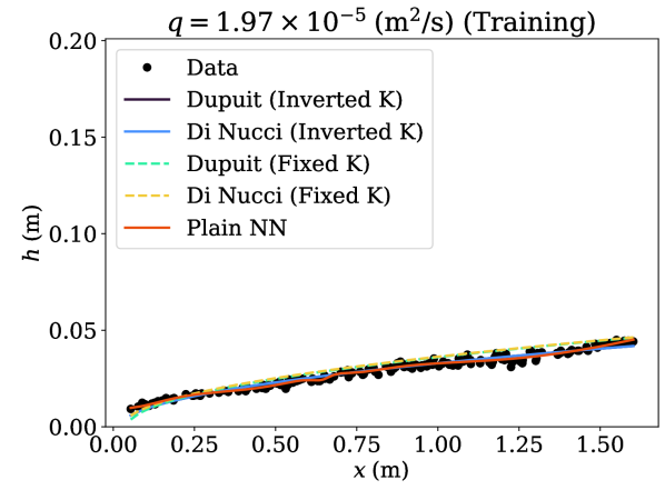
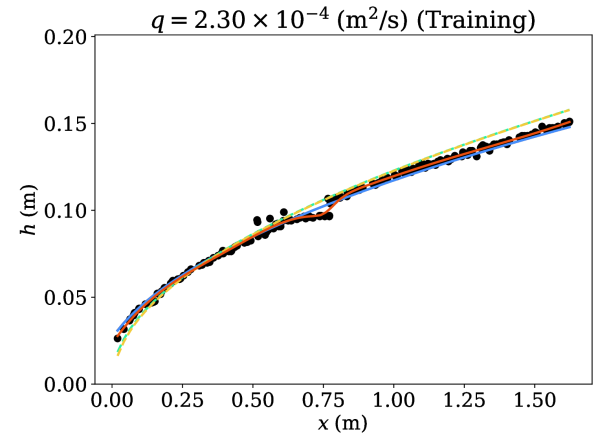
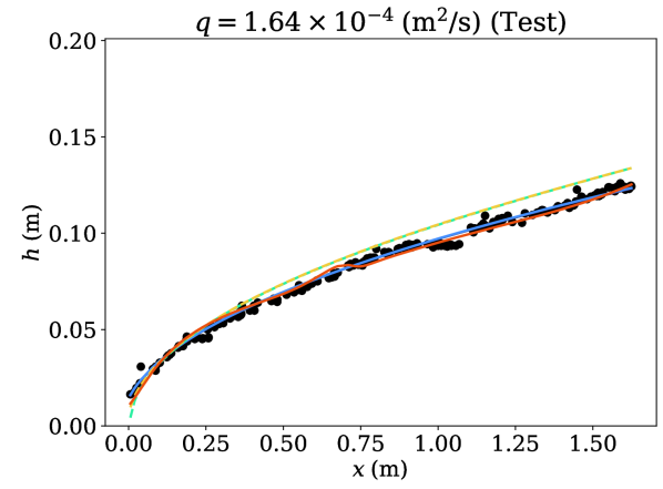
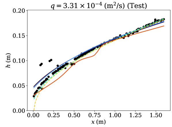
Figure 17: Neural network predictions of free surface profiles for the experimental data using 2 mm beads.

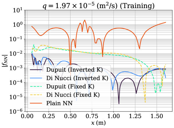
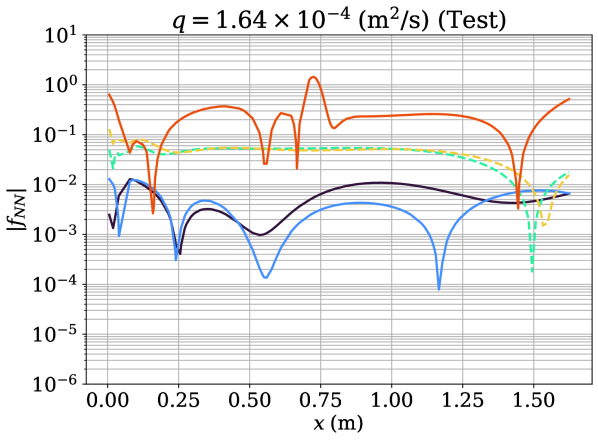
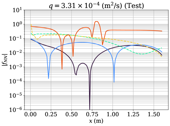
Figure 18: The PDE residuals inside the domain corresponding to free surface profile predictions for 2 mm bead size, shown in Figure 17.

7.2 Inversion of Hydraulic Conductivity

PINNs predictions for inverted $K$ performs very well near the seepage face boundary but slightly deviate from the test data away from the boundary, as shown in Figures 15 and 17 for Dupuit and Di Nucci models respectively. We also present the inverted values of hydraulic conductivity for both the 1 mm and 2 mm cases in Table 2. The recovered values of $K$ compare well with their corresponding theoretical estimates, there is still a deviation in the inverted values due to the discrepancy between theory and experiments.

The corresponding PDE residuals, across the domain, are shown in Figures 16 and 18 for Dupuit and Di Nucci cases. It can be observed that the PDE residual for the inverted values of $K$ is lower than both for fixed $K$ and for plain neural network and is less than $10^{-1}$ on almost all cases.

	Hydraulic conductivity $K$ (m/s)
1 mm beads
Calculated	0.00910
Di Nucci	0.00786
Dupuit	0.00783
2 mm beads
Calculated	0.0285
Di Nucci	0.0355
Dupuit	0.0355

Table 2: Comparison of inverted and a-priori estimates of $K$ from experimental data.

7.3 Comparison of terms

We also train individual PINNs on each flow profile, inverting for $K$ using the Di Nucci equation as the regularizing equation. Using the resulting neural networks, we again compare the relative sizes of the horizontal and vertical flow terms in the Di Nucci equation. These are presented in Figure 19 for 1 mm and 2 mm beads respectively. Only the minimum and maximum $\Pi$ values observed in our experimental apparatus are shown. Since $\Pi$ lies in range $\mathcal{O}(10^{-3})-\mathcal{O}(10^{-2})$, higher order vertical flow effects are not dominant in the domain. So, as seen earlier for synthetic data, the first order term $-\frac{K}{q}hh_{x}$ has the major contribution.

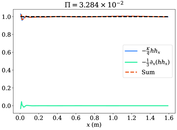
(a) 1 mm beads

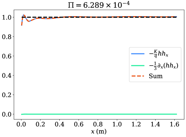
(b) 2 mm beads

Figure 19: PDE terms computed from the trained neural networks for the experimental data.

8 Discussion

Di Nucci’s momentum equation is useful to evaluate the relative contribution of vertical and horizontal flow effects. Scaling it provides a dimensionless number, $\Pi=2q/KL$, which is the ratio of vertical to horizontal flow effects. For $\Pi\leq 0.1$, the Dupuit model is a good approximation. However, higher order vertical flow effects need to be considered for $\Pi>0.1$ through Di Nucci model. Although our experimental measurements were restricted to $\Pi\leq 0.1$ case, the synthetic data revealed the full spectrum of cases.

PINNs robustly predict the hydraulic conductivity from the data. The deviations of inverted values of hydraulic conductivity from the theoretical estimates can be due to many reasons, the most important being the difference in theory from experimental data. This is likely a combination of experimental error and the empirical nature of the theory. We believe the inverted values of $K$ are more accurate than those calculated. Also, this is a novel way of measuring the hydraulic conductivity through contactless measurements compared with permeameters. As an extension to this work, instead of constant permeability, a 2D permeability field $K(\textbf{x})$ and moreover boundary conditions can be inverted for either separately or jointly.

As a method of learning flow profiles from experimental data, PINNs requires less training data compared to a conventional neural network due to physics based constraints on the solution space. The PDE based regularization makes it less sensitive to the noise in data. PINNs use information from both the data and the model PDE, which can be a simple model such as Dupuit-Boussinesq equation. It is well known that Dupuit model neglects the vertical flow effects as well as seepage face development. By considering the information from the data, the seepage face height and lake-level dynamics can be considered.

PINNs is also able to improve upon the predictions given by solving the PDE alone. It is recognized that models such as the Dupuit-Boussinesq approximation and even the Di Nucci equations do not fully represent the physics in the system. Thus, PINNs improves upon such predictions by combining the PDE information with experimental data, without the resorting to more complex and computationally expensive models. Furthermore, as it is difficult to prescribe appropriate boundary conditions for flows with seepage faces, we cannot make predictions directly using the PDE in these circumstances. However, we are able to make use of the information provided by PDE through the PINNs formulation to make predictions as well as infer the hydraulic conductivity from experimental data. This showcases an important application area for PINNs in groundwater flows.

9 Conclusions

In this paper, we have investigated steady groundwater flow using Physics Informed Neural Networks. The free-surface profile data comes from analytical results of Dupuit-Boussinesq and Di Nucci models and moreover, laboratory experiments. PINNs predict the free surface profiles very well on both training and test data which are less sensitive to noise. The conventional neural network gives oscillatory and unphysical results on the same data set, due to lack of physics information. An optimal value of PDE misfit regularization parameter has been found using scaling as well as L-curve analysis on synthetic data which performs very well on the experimental data. Further, hydraulic conductivity has been inverted for the training data which gives fairly accurate predictions of free-surface profiles and is close to the theoretical estimates. Then we compared the Di Nucci and Dupuit-Boussinesq models PDEs directly on the synthetic as well as experimental data. We found a dimensionless number $\Pi=2q/KL$ representing the effect of vertical flow to the horizontal flow by scaling the Di Nucci model. Using automatic differentiation capabilities of neural networks, we found that for $\Pi\leq 0.1$, horizontal flow dominates across the domain which can be easily modeled by Dupuit-Boussineq equation. Otherwise, Di Nucci model needs to be considered. In future, we plan to extend this PINNs model to study transient groundwater flow dynamics.

Appendix A Scaling analysis

The boundary value problem (5) in Di Nucci’s model is rewritten below

$$-\frac{\partial}{\partial x}\Bigg{[}\frac{h^{2}}{2}-\frac{1}{K}\frac{\partial}{\partial x}\bigg{(}\frac{q}{h}\bigg{)}\frac{h^{3}}{3}\Bigg{]}=\frac{q}{K},$$ (37)

subject to boundary conditions:

$$h(L,t) =H=\textrm{constant},$$ (38)

$$\frac{q}{K}(L,t) =g(t).$$ (39)

It can be recasted into dimensionless form using the dimensionless variables $x^{\prime}$ for x-coordinate, $h^{\prime}$ for free-surface height and $q^{\prime}$ for flux,

$$x^{\prime}=\frac{x}{L},\quad h^{\prime}=\frac{h}{H},\quad q^{\prime}=\frac{q}{q_{c}}$$ (40)

where $q_{c}$ is the constant characteristic flux. Plugging them into (37) gives

$$\frac{q_{c}q^{\prime}}{K}=-\frac{1}{L}\frac{\partial}{\partial x^{\prime}}\left[\frac{H^{2}}{2}h^{\prime 2}-\frac{q_{c}h_{c}^{3}}{HKL}\frac{\partial}{\partial x^{\prime}}\left(\frac{q^{\prime}}{h^{\prime}}\right)\frac{h^{\prime 3}}{3}\right].$$ (41)

Dividing by $K/q_{c}$, we get

$$q^{\prime} =-\frac{K}{q_{c}L}\frac{\partial}{\partial x^{\prime}}\left[\frac{H^{2}}{2}h^{\prime 2}-\frac{q_{c}H^{3}}{HKL}\frac{\partial}{\partial x^{\prime}}\left(\frac{q^{\prime}}{h^{\prime}}\frac{h^{\prime 3}}{3}\right)\right]$$ (42)

$$=-\frac{\partial}{\partial x^{\prime}}\left[\frac{KH^{2}}{2q_{c}L}h^{\prime 2}-\left(\frac{H}{L}\right)^{2}\frac{\partial}{\partial x^{\prime}}\left(\frac{q^{\prime}}{h^{\prime}}\right)\frac{h^{\prime 3}}{3}\right].$$ (43)

As a result, we get two dimensionless numbers

$$\Pi_{1}=\frac{KH^{2}}{2q_{c}L}\quad\textrm{and}\quad\Pi_{2}=\left(\frac{H}{L}\right)^{2}.$$ (44)

The equation (43) transforms into a dimensionless PDE becomes

$$q^{\prime} =-\frac{\partial}{\partial x^{\prime}}\left[{\Pi_{1}h^{\prime 2}}-{\Pi_{2}\frac{\partial}{\partial x^{\prime}}\left(\frac{q^{\prime}}{h^{\prime}}\right)\frac{h^{\prime 3}}{3}}\right].$$ (45)

On the RHS of (45), the first term refers to the quasi-1D horizontal flux from Dupuit-Boussinesq model and the second term represents the higher order vertical flow effects considered in the Di Nucci model. The ratio of the two dimensionless numbers $\Pi$ thus provides ratio of the vertical flow effects to the horizontal flux stemming from the lubrication approximation ($H/L<<1$), where

$$\Pi=\frac{\Pi_{2}}{\Pi_{1}}=\frac{\left(\frac{H}{L}\right)^{2}}{\frac{KH^{2}}{2q_{c}L}}=\frac{2q_{c}}{KL}.$$ (46)

For the steady-state case, $q_{c}$ is a constant $q$ given by $q=K\frac{H^{2}-h_{l}^{2}(\infty)}{2L}$ from relation (13), therefore

$$\Pi=\frac{2q}{KL}=\left(\frac{H}{L}\right)^{2}-\left(\frac{h_{l}(\infty)}{L}\right)^{2}.$$ (47)