Degree-of-Freedom of Modulating Information in the Phases of Reconfigurable Intelligent Surface

Abstract

This paper investigates the information theoretical limit of a reconfigurable intelligent surface (RIS) aided communication scenario in which the RIS and the transmitter either jointly or independently send information to the receiver. The RIS is an emerging technology that uses a large number of passive reflective elements with adjustable phases to intelligently reflect the transmit signal to the intended receiver. While most previous studies of the RIS focus on its ability to beamform and to boost the received signal-to-noise ratio (SNR), this paper shows that if the information data stream is also available at the RIS and can be modulated through the adjustable phases at the RIS, significant improvement in the degree-of-freedom (DoF) of the overall channel is possible. For example, for an RIS system in which the signals are reflected from a transmitter with $M$ antennas to a receiver with $K$ antennas through an RIS with $N$ reflective elements, assuming no direct path between the transmitter and the receiver, joint transmission of the transmitter and the RIS can achieve a DoF of $\min(M+\frac{N}{2}-\frac{1}{2},N,K)$ as compared to the DoF of $\min(M,K)$ for the conventional multiple-input multiple-output (MIMO) channel. This result is obtained by establishing a connection between the RIS system and the MIMO channel with phase noises and by using results for characterizing the information dimension under projection. The result is further extended to the case with a direct path between the transmitter and the receiver, and also to the multiple access scenario, in which the transmitter and the RIS send independent information. Finally, this paper proposes a symbol-level precoding approach for modulating data through the phases of the RIS, and provides numerical simulation results to verify the theoretical DoF results.

I Introduction

Reconfigurable intelligent surface (RIS), also known as the intelligent reflective surface (IRS), is a promising new technology that utilizes a large number of reflective elements with adjustable phase shifts to enhance the spectrum and energy efficiencies of wireless communication systems [2, 3, 4, 5]. In most of the current literature, the RIS is envisioned to be used as a passive beamformer with the reflective coefficients being configured for maximizing the received signal-to-noise ratio (SNR) of the overall channel. Passive beamforming, however, does not fully harvest the potentials of the RIS. The goal of this paper is to show that if the information data stream is available at the RIS, it is possible to use the RIS to modulate the information through phase shifts. In effect, the adjustable reflective coefficients can be used not only to enhance the channel, but also to carry information.

This paper aims to show that modulating information through phases allows the RIS to significantly enhance the degree-of-freedom (DoF), also known as the multiplexing gain, of the overall channel between the transmitter and the receiver. The gains in DoF from modulating information through the phases of the RIS are quantified both for the cases with and without cooperation between the transmitter and the RIS. The former case corresponds to the point-to-point multiple-input multiple-output (MIMO) channel where the RIS helps the transmitter send the same data, while the latter case corresponds to the a multiple access channel where the RIS and the transmitter send independent data which are jointly decoded at the receiver.

Moreover, this paper proposes a symbol-level precoding strategy for the joint transmission of information from the transmitter and the RIS to the receiver. We show that such a strategy can approach the achievable information theoretic DoF of the overall system.

I-A Prior Works

RIS can be thought of as an array of a large number of reflective elements, each of which can induce a phase shift between the incident signal and the reflecting signal. By adjusting the phase shifts, the RIS can enhance the transmission quality of the overall channel by adaptively beamforming the incident signal to an intended reflecting direction [6]. As compared to traditional relaying techniques [7, 8], the RIS reflects the incident signal passively, so it has much lower energy consumption. Further, by utilizing a large number of analog reflective elements and by adjusting their phases in real time, the RIS can achieve a high beamforming gain at relatively low hardware cost.

Because of the above promising advantages, the applications of RIS for enhancing wireless communication systems have been extensively investigated in the literature. Most of the existing literature on the RIS-aided wireless communication system focuses on the optimization of the phase shifts at the RIS to improve various system-level objectives e.g., for energy minimization [9], maximizing the minimum signal-to-interference-plus-noise ratio (SINR) [9], for sum-rate maximization for both single-cell [10] and multi-cell [11] scenarios, for utility maximization using a machine learning approach [12], as well as for various scenarios such as the wideband orthogonal frequency division multiplexing (OFDM) system [13], the millimeter-wave (mmWave) system [14, 15], and the multiple RIS systems [16]. These existing studies, however, utilize the RIS only as a passive analog beamformer to achieve an SNR gain. Passive analog beamforming works by adjusting the phase shifts of scattered wavefronts at different reflective elements so that they add constructively at the receiver, thereby enhancing the SNR at the receiver. For these systems, the phase shifts at the RIS are functions of the instantaneous channel realizations only.

The main focus of this paper is to explore the possibility that if, in addition to the channel state information (CSI), the RIS also has access to the data, then the RIS can modulate the information stream in the phase shifts to further enhance the capacity of the overall communication channel. By modulating information using the RIS, the information is essentially being conveyed by changing the transmission environment.

The idea of modulating information through the transmission environment has been considered by several earlier works under different names, e.g. media-based communication [17] and load modulated arrays [18]. But an exact analysis of the information theoretic limits of such systems is a challenging task. In the RIS context, this idea has been previously explored in [19], which studies the information theoretic achievable rate for joint information transmission by the transmitter and the RIS, but under the restrictive assumption that the RIS operates with a fixed finite modulation. Information transmission through RIS has also been considered in [20] and [21], which primarily focus on the design of decoding algorithms when extra information bits are carried in the RIS. In general, the information theoretical limit of modulating through RIS has not been fully characterized.

I-B Main Contributions

This paper aims to characterize the DoF, or the multiplexing gain, or the pre-log factor, of a wireless transmission system equipped with an RIS in which information is modulated through the phase shifts. We study both the case in which the information bits are jointly encoded in the transmit radio frequency (RF) signal and the phase shifts at the RIS for an intended MIMO receiver, as well as the case in which the RIS and the RF transmitter send independent information, corresponding to a multiple access channel.

The DoF is an important metric which captures the high SNR asymptotic behavior of channel capacity for channels with additive Gaussian noises. The main challenge in the analysis of the RIS channel lies in the multiplicative nature of the channel model in which the received signal is the product of two different information-carrying signals. We tackle this challenge by connecting the achievable rate of the RIS channel to the capacity of the MIMO channel with phase noises. Tools for studying the information dimension and the point-wise dimension under projection are used.

For an RIS system consisting of a transmitter with $M$ transmit antennas, a receiver with $K$ receive antennas, and an RIS with $N$ reflective elements, the main results of this paper show that:

• For the case of joint transmission by the RF transmitter and the RIS, a DoF of $\min(M+\frac{N}{2}-\frac{1}{2},N,K)$ for the overall channel can be achieved, assuming that the direct path between the transmitter and the receiver is blocked. The $1/2$ factor corresponds to the phase ambiguity between the RF signal and the RIS phase shifts.

• When there is a direct path with channel rank $r>0$, the DoF of joint transmission is $\min(M+\frac{N}{2},N+r,K)$.

• The above results imply that as compared to a conventional MIMO channel with $M$ transmit antennas and $K$ receive antennas achieving a DoF of $\min(M,K)$, in the case of $M<K$, a cooperative RIS can significantly improve the overall channel capacity by allowing modulating data through the phase shifts.

• When the RF transmitter and the RIS send independent information, the same sum DoF can also be achieved as the above joint transmission case. This means that if there are more receive antennas than transmit antennas, the RIS can embed additional data streams in the phase shifts without affecting the DoF of the direct transmission.

• A symbol-level precoding strategy is proposed as an practical implementation of jointly encoding information by the RF transmitter and the RIS. It is shown to approach the information theoretic maximum DoF of joint transmission.

I-C Paper Organization and Notation

The rest of the paper is organized as follows. Section II describes the channel model for the RIS system. Section III discusses the RIS model without a direct path and provides the DoF result for both the joint transmission case and the multiple access case. These results are extended to the case where the direct path is present in Section IV. Practical implementation of the joint transmission strategy via symbol-level precoding is discussed in Section V. Numerical results are presented in Section VI. Conclusions are drawn in VII.

The notations used in the paper are as follows. Lower-case letters are used to denote scalars; upper-case letters are used to denote random variables. Bold-faced letters are vectors. Bold-faced upper-case letters are either random vectors, or matrices, where the context should make it clear. Exceptions to the above are the dimensions of the transmitter, the RIS, and the receiver vectors, which are denoted as $M$, $N$, and $K$, respectively. The capacity of a channel with power constraint $P$ is denoted as $C(P)$. Finally, we use $\mathcal{CN}(\cdot,\cdot)$ to denote the circularly symmetric complex Gaussian distribution and $\operatorname{Unif}(\cdot)$ to denote the uniform distribution.

II System Model and Problem Formulation

II-A Channel Model

The RIS-aided communication scenario is as shown in Fig. 1, where an RIS with $N$ reflective elements is deployed between an $M$-antenna transmitter and a $K$-antenna receiver. Let ${\mathbf{H}\in\mathbb{C}^{N\times M}}$, ${\mathbf{G}\in\mathbb{C}^{M\times N}}$, $\mathbf{F}\in\mathbb{C}^{K\times M}$ be the channel response matrices from the transmitter to the RIS, from the RIS to the receiver, and from the transmitter to the receiver respectively, which are assumed to be fixed and known everywhere, i.e., at the transmitter, the RIS controller, and the receiver. The channels can be estimated, e.g., using methods in [22, 23].

We assume that each element of the RIS combines all the transmitted signals at a single point and reflects it from this point to the receiver with an adjustable phase shift. The discrete-time channel model for the communication scenario is given by

$$\mathbf{Y}=\sqrt{P}\left(\mathbf{H}{\boldsymbol{\Theta}}\mathbf{G}+\mathbf{F}\right)\mathbf{X}+\mathbf{Z},$$ (1)

where $\mathbf{Y}\in\mathbb{C}^{K}$ is the received signal vector, $\mathbf{X}\in\mathbb{C}^{M}$ is the transmit signal vector normalized by the power constraint $P$ so that

$$\mathbb{E}[\|\mathbf{X}\|_{2}^{2}]\leq 1,$$ (2)

and $\mathbf{Z}\sim\mathcal{CN}(0,\sigma^{2}\mathbf{I}_{K})$ is the additive Gaussian noise vector at the receiver. Here, ${\bm{\Theta}}$ is the $N\times N$ reflecting coefficient matrix induced by RIS taking the form of

$${\bm{\Theta}}={\text{diag}}([e^{j\theta_{1}},e^{j\theta_{2}},\cdots,e^{j\theta_{N}}]),$$ (3)

where ${\theta}_{m}$ is the phase-shifting coefficient of the $m$-th reflective element on the RIS and ${\text{diag}}(\cdot)$ denotes a diagonal matrix whose diagonal elements are given by the corresponding entries of the argument. Implicit in this discrete-time channel model is the assumption that the transmitter and the RIS operate at the same symbol rate.

An important special case of model (1) is when the direct path from the transmitter to the receiver is blocked, i.e. $\mathbf{F}=\mathbf{0}$. In this case, model (1) reduces to

$$\mathbf{Y}=\sqrt{P}\mathbf{H}\underbrace{{\boldsymbol{\Theta}}\mathbf{G}\mathbf{X}}_{\mathbf{W}}+\mathbf{Z}.$$ (4)

Model (4) is easier to analyze. This paper begins by focusing on model (4); the more general model (1) is treated in the second half of the paper. For convenience, we define $\mathbf{W}=\mathbf{\Theta GX}$ as shown in (4) so that the output of the RIS is $\sqrt{P}\mathbf{W}$.

II-B RIS as Passive Beamformer

In the conventional model, the RIS is used as as a passive beamformer to improve the overall transmission quality. In this case, the system design problem is simply that of finding $\mathbf{\Theta}$ as a function of $\mathbf{H}$ and $\mathbf{G}$ in order to maximize the over channel capacity from $\mathbf{X}$ to $\mathbf{Y}$. Mathematically, this maximization operation can be written as

$$\max_{\boldsymbol{\Theta}}\max_{p(\mathbf{x})}I\left(\mathbf{X};\mathbf{Y}|\boldsymbol{\Theta}\right),$$ (5)

subject to the constraints (2) and (3). In this case, the reflecting coefficients do not carry any information. The main function of the RIS is to enhance the beamforming gain from $\mathbf{X}$ to $\mathbf{Y}$, i.e. to increase the received SNR at the receiver.

Instead of using the RIS as a conventional beamformer, this paper explores the potential of using the RIS to encode information in the reflective coefficients themselves. Toward this end, we consider two scenarios below.

II-C Joint Transmission Model

The first scenario considered in this paper is the case in which the RIS cooperates with the transmitter to transmit a single data stream. This is equivalent to a point-to-point channel from $\mathbf{(X,\Theta)}$ to $\mathbf{Y}$. The capacity of such a channel, as a function of the transmitted power $P$, can be written as

$$C(P)=\max_{p(\mathbf{x},\boldsymbol{\Theta})}I(\mathbf{X},\boldsymbol{\Theta};\mathbf{Y}),$$ (6)

subject to the constraints (2) and (3). This is referred to as the joint transmission model and is considered in the first part of this paper.

Computing $I(\mathbf{X},\boldsymbol{\Theta};\mathbf{Y})$ is not an easy task as it involves a multi-dimensional integration over the probability density functions (pdf) of $\mathbf{X}$ and $\boldsymbol{\Theta}$, which can only be done numerically. To obtain some insight into the problem, in this paper, we characterize the DoF of this channel model, which is defined as the pre-log factor of the rate as $P\rightarrow\infty$, i.e.

$$\mathrm{DoF}_{(\mathbf{X,\Theta})}\triangleq\lim_{P\rightarrow\infty}\frac{C(P)}{\log P}.$$ (7)

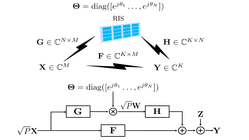
Figure 1: Channel model for a RIS assisted point-to-point MIMO communication system in which $(\mathbf{X},\mathbf{\Theta})$ jointly transmit as an input to the channel

II-D Multiple Access Model

The second scenario considered in this paper is the case in which the transmitter and the RIS each send an independent data stream to the receiver, and there is no cooperation between the two. This is referred to as the multiple access model.

Although the channel remains the same as in the joint transmission case, because there is no cooperation between $\mathbf{X}$ and $\boldsymbol{\Theta}$ in the multiple access model, the input distributions are constrained to be the product of the marginal distributions $p(\mathbf{X})$ and $p(\mathbf{\Theta})$. Denote the achievable rate of $\mathbf{X}$ from the transmitter as $R_{\mathbf{X}}$ and the achievable rate of $\boldsymbol{\Theta}$ from the RIS as $R_{\boldsymbol{\Theta}}$. The capacity region of the multiple access channel is the closure of the convex hull of all ($R_{\mathbf{X}}$, $R_{\boldsymbol{\Theta}}$) satisfying

$$R_{\mathbf{X}} \leq I(\mathbf{X};\mathbf{Y}|\boldsymbol{\Theta}),$$ (8)

$$R_{\boldsymbol{\Theta}} \leq I(\boldsymbol{\Theta};\mathbf{Y}|\mathbf{X}),$$ (9)

$$R_{\mathbf{X}}+R_{\boldsymbol{\Theta}} \leq I(\mathbf{X},\boldsymbol{\Theta};\mathbf{Y}).$$ (10)

for some joint distributions $p(\mathbf{X})p(\boldsymbol{\Theta})$ subject to the constraints (2) and (3).

The capacity region is a function of the transmit power $P$. A DoF pair $(\mathrm{DoF}_{\mathbf{X}},\mathrm{DoF}_{\boldsymbol{\Theta}})$ is achievable if there exists a sequence of rate pairs $(C_{\mathbf{X}}(P),C_{\boldsymbol{\Theta}}(P))$ on the boundary of the capacity region, indexed by $P$, such that

$$\mathrm{DoF}_{\mathbf{X}} = \displaystyle\lim_{P\rightarrow\infty}\frac{C_{\mathbf{X}}(P)}{\log P},$$ (11)

$$\mathrm{DoF}_{\boldsymbol{\Theta}} = \displaystyle\lim_{P\rightarrow\infty}\frac{C_{\boldsymbol{\Theta}}(P)}{\log P}.$$ (12)

The closure of the convex hull of all achievable DoF pairs defines the DoF region of the multiple access model.

The goal of this paper is to characterize the DoF of the joint transmission and the DoF region of the multiple access model.

III DoF of RIS System without Direct Path

We begin by considering the RIS model (4) without the direct path. The aim is to characterize both the DoF of the joint transmission case, where $\mathbf{X}$ and $\mathbf{\Theta}$ jointly transmit information to the receiver $\mathbf{Y}$, and the multiple access case, where $\mathbf{X}$ and $\mathbf{\Theta}$ are independent users.

A key observation is that the RIS channel model is closely related to additive white Gaussian noise (AWGN) channel with phase noise. To illustrate this idea, we start with the single-input single-output (SISO) channel as an example, then move onto the MIMO case.

III-A Joint Transmission in SISO Channel with $(X,\theta)$ as Input

Consider the special case of $M=N=K=1$, for which the signal model (4) reduces to

$$Y = \sqrt{P}e^{j\theta}X+Z$$ (13)

$$= \sqrt{P}|X|e^{j(\angle X+\theta)}+Z,$$ (14)

where $Z\sim\mathcal{CN}(0,\sigma^{2})$, and the channel gain is omitted for simplicity. The input constraints are $\theta\in(-\pi,\pi]$ and $\mathbb{E}|X|^{2}\leq 1$. Here, we use $|\cdot|$ to denote the amplitude and $\angle$ as the phase of a complex number.

The capacity for joint transmission is the maximum mutual information between the input $(X,\theta)$ and the output $Y$. This mutual information can be decomposed as

$$I(X,\theta;Y)=I(X;Y)+I(\theta;Y|X).$$ (15)

Assume that we choose $p(\theta)\sim\operatorname{Unif}(-\pi,\pi]$ and let $X$ and $\theta$ be independent. Consider the first term $I(X;Y)$. Since $\theta$ is completely unknown, the channel from $X$ and $Y$ is in effect a non-coherent channel [24], in which $\theta$ can be thought of as phase noise. For such a phase-noise channel, information can only be conveyed through the magnitude, so we have

$$I(X;Y)=I(|X|;|Y|).$$ (16)

The optimal distribution of the magnitude $|X|$ for maximizing $I(|X|;|Y|)$ is known to be discrete [24, Theorem 5]. However, setting $X$ as Gaussian can be shown to give the same DoF [25]. The achievable rate using Gaussian input in the high SNR regime can be approximated as [26, 24]

$$I(|X|;|Y|)\approx\frac{1}{2}\log\left(\frac{P}{\sigma^{2}}\right)-0.69.$$ (17)

Thus, the $I(X;Y)$ term achieves a DoF of $1/2$.

Now, consider the second term $I(\theta;Y|X)$, where $X$ is known and can be considered as part of the channel gain. In this case, only the phase $\theta$ carries information. This is known as the constant-intensity channel, or constant-envelope channel, or ring modulation [25, 27]. Intuitively, the input is a phase-shift keying (PSK) modulation. The asymptotic approximation of the capacity of such a channel is found in the high SNR limit in [26, eqn. (25)] and is given by

$$\max_{p(\theta)}I(\theta;Y|X) \approx\frac{1}{2}\log\left(\frac{P|X|^{2}}{\sigma^{2}}\right)+1.1$$

$$=\frac{1}{2}\log\left(\frac{P}{\sigma^{2}}\right)+\log|X|+1.1,$$ (18)

where the optimal distribution of $\theta$ is uniform in $(-\pi,\pi]$. Since we have $\mathbb{E}|X|^{2}\leq 1$, the $\log|X|$ term cannot scale with SNR. Thus, the $I(\theta;Y|X)$ term also achieves a DoF of $1/2$.

Combining the two terms, we see that for the SISO channel, the joint transmission of $(X,\theta)$ achieves the same sum DoF as that of a conventional AWGN channel without RIS.

For the AWGN channel without RIS, the DoF of 1 can be thought of as being comprised of $1/2$ DoF in the magnitude and $1/2$ DoF in the phase. But with RIS as part of the channel, there is $1/2$ DoF overlap between the phase of the input and the phase of the RIS. Thus, the joint transmission of $X$ and $\theta$ achieves the same $1/2$ DoF in magnitude and $1/2$ DoF in phase.

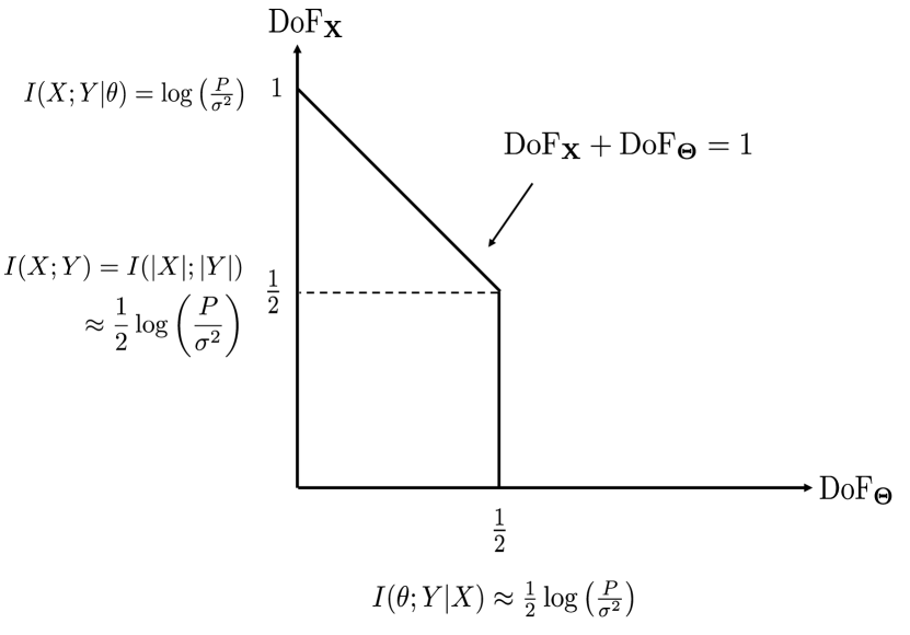
Figure 2: DoF region of the SISO multiple-access channel model

The above argument can be extended to the multiple access setting with $X$ and $\theta$ as independent inputs. The DoF region of such an SISO multiple access channel is as shown in Fig. 2.

III-B Joint Transmission in MIMO Channel with $(\mathbf{X},\mathbf{\Theta})$ as Input

We now consider the MIMO case for the joint transmission of $\mathbf{X}$ and $\mathbf{\Theta}$, and with arbitrary $M$, $N$, and $K$, and compute the DoF of $I(\mathbf{X},\boldsymbol{\Theta};\mathbf{Y})$, but assuming that there is no direct path between $\mathbf{X}$ and $\mathbf{Y}$. This result will be generalized to the case with direct path later, but the model without the direct path is also of independent interest, because in many cases the RIS is deployed where the direct path between the transmitter and the receiver is blocked.

The main result below, which is for the point-to-point case with $(\mathbf{X},\mathbf{\Theta})$ jointly transmitting as the input to channel, is also used later as a tool for showing the DoF region of the multiple access case.

Theorem 1

Consider the channel model

$$\mathbf{Y}=\sqrt{P}\mathbf{HW}+\mathbf{Z}=\sqrt{P}{\mathbf{H}\boldsymbol{\Theta}\mathbf{G}}\mathbf{X}+\mathbf{Z},$$ (19)

with $(\mathbf{X,\Theta})$ as the input where $\mathbf{X}\in\mathbb{C}^{M}$ has a power constraint $\mathbb{E}[\|\mathbf{X}\|_{2}^{2}]\leq 1$ and ${\boldsymbol{{\Theta}}}={\text{diag}}([e^{j\theta_{1}},e^{j\theta_{2}},\cdots,e^{j\theta_{{N}}}])$, and $\mathbf{Y}\in\mathbb{C}^{K}$ as the output, and $\mathbf{Z}\sim\mathcal{CN}(0,\mathbf{I}_{K})$ as the noise. For almost all matrices $\mathbf{G}\in\mathbb{C}^{N\times M}$, $\mathbf{H}\in\mathbb{C}^{K\times N}$, the maximum DoF is

$$\mathrm{DoF}_{(\mathbf{X},\mathbf{\Theta})}=\min\left(M+\frac{N}{2}-\frac{1}{2},N,K\right).$$ (20)

This maximum DoF can be achieved using any of the following distributions with independent $\mathbf{X}$ and $\mathbf{\Theta}$:

1. $\mathbf{X}\sim\mathcal{CN}(0,\mathbf{I}_{M})$ and $\boldsymbol{\Theta}$ with $\theta_{i}\sim\operatorname{Unif}(-\pi,\pi]$.

2. The distribution of $\mathbf{X}$ is chosen such that the first $M-1$ elements are i.i.d. complex Gaussian, i.e., $\mathbf{X}_{M-1}\sim\mathcal{CN}(0,\mathbf{I}_{M-1})$, and $X_{M}$ is chosen to be real with a chi-squared distribution with 2 degrees of freedom. The distribution of $\boldsymbol{\Theta}$ is $\theta_{i}\sim\operatorname{Unif}(-\pi,\pi]$.

3. The distribution of $\mathbf{X}$ is i.i.d. complex Gaussian for all $M$ elements, i.e., $\mathbf{X}\sim\mathcal{CN}(0,\mathbf{I}_{M})$. For $\mathbf{\Theta}$, the first ${N}-1$ elements of $\boldsymbol{\Theta}$ are chosen as uniform distribution with $\theta_{i}\sim\operatorname{Unif}(-\pi,\pi],~{}i=1,\ldots,N-1$, and the last element of $\boldsymbol{\Theta}$ is fixed as 1, i.e., $\theta_{N}=1$.

Proof:

The proof is based on an equivalence between information dimension and the DoF of an additive noise channel. Toward this end, we first compute the information dimension of the output $\mathbf{W}$ at the RIS. This is accomplished by building a connection between the channel model with RIS and the MIMO channel with phase noise. We then compute the information dimension of $\mathbf{HW}$ by studying the behavior of information dimension under projection. The details of the proof are in Appendix A. ∎

We now give an interpretation of the DoF result (20) in Theorem 1. The channel model has two inputs: $\mathbf{X}$ of dimension $M$, and $\mathbf{\Theta}$ of dimension $N$. Because $\mathbf{\Theta}$ has phase control only, its information dimension is $\frac{N}{2}$. Further, $\mathbf{X}$ and $\mathbf{\Theta}$ have $1/2$ dimension overlap, due to the product form of the channel model, which leaves a common phase ambiguity between $\mathbf{X}$ and $\mathbf{\Theta}$. In other words, it is not possible to resolve the phases of $\mathbf{X}$ and $\mathbf{\Theta}$ individually, but only the phase of their product. For this reason, the total input dimension is $M+\frac{N}{2}-\frac{1}{2}$.

Moreover, the channel has output $\mathbf{Y}$ of dimension $K$, and the RIS acts as a relay with a bottleneck $\mathbf{W}$ of dimension $N$. The overall DoF must be the minimum of the input dimension, the relay dimension, and the output dimension. This is why the multiplexing gain is $\min(M+\frac{N}{2}-\frac{1}{2},N,K)$.

The key observation here is the $1/2$ dimension overlap between $\mathbf{X}$ and $\mathbf{\Theta}$. It is for this reason that the maximum overall DoF can be achieved with not only a choice of input distributions with $\mathbf{X}\sim\mathcal{CN}(0,\mathbf{I}_{M})$ and $\boldsymbol{\Theta}$ with $\theta_{i}\sim\operatorname{Unif}(-\pi,\pi]$, but also with $1/2$ dimension removed from either $\mathbf{X}$ or $\mathbf{\Theta}$. In particular, Theorem 1 shows that fixing the phase of the last element of either $\mathbf{X}$ or $\boldsymbol{\Theta}$ still allows the same DoF to be achieved. In fact due to symmetry, the same result holds true if we fix any of one phase value in either $\mathbf{X}$ or $\mathbf{\Theta}$.

An important implication of Theorem 1 is that as compared to a MIMO channel with $M$ antennas at the input and $K$ antennas at the output achieving a DoF of $\min(M,K)$, an RIS can improve the overall DoF if $K>M$, and $N>\min(M,K)$. In essence, the phase shifts at the RIS can act as part of the input to effectively increase the total input dimensions. Thus, by making the input data available to the RIS, we are enabling the RIS to help the transmitter modulate the data stream via the phase shifts. Assuming that $N$ is much larger than $M$ and $K$ as in typical deployment scenarios, the maximum additional number of data streams that the RIS can provide is $\frac{N}{2}-\frac{1}{2}$. Note that if the RIS is used merely as a beamformer or as a reflector, it cannot improve the DoF. Thus, modulating data through phase shifts has significant advantage.

A practical case is when the transmitter has a single radio-frequency (RF) chain. This is akin to using the RIS to emulate a MIMO transmitter, i.e., a single-antenna active transmitter together with an RIS can be jointly configured to act as a MIMO array. Such a system can be considered as a low-cost alternative to a fully digital MIMO system. In this case, we have $M=1$ and the signal model is given by

$$\mathbf{Y}=\mathbf{H}{\boldsymbol{\Theta}}\mathbf{g}X+\mathbf{W},$$ (21)

Assuming an RIS with large $N$, Theorem 1 implies that the overall DoF is $K$. One possible way of achieving this DoF is to use the amplitude of $X$ to modulate $\frac{1}{2}$ DoF and to use a RIS of size at least $N=2K-1$ to modulate the remaining $(K-\frac{1}{2})$ DoF.

III-C MIMO Channel with Deterministic $\mathbf{X}$

We can carry the example in the previous section one step further and consider a system in which the information is modulated only from the RIS via $\mathbf{\Theta}$ and not by the transmitter at all. In this case, the transmitter sends a deterministic signal $\mathbf{X}$ (which carries no information) and the channel model becomes

$$\mathbf{Y} =\sqrt{P}\mathbf{H}\boldsymbol{\Theta}\mathbf{G}\mathbf{X}+\mathbf{Z}$$ (22)

$$=\sqrt{P}\mathbf{H}\mathrm{diag}(\mathbf{G}\mathbf{X})\boldsymbol{\Phi}+\mathbf{Z}$$ (23)

$$=\sqrt{P}\bar{\mathbf{H}}\boldsymbol{\Phi}+\mathbf{Z},$$ (24)

where $\boldsymbol{\Phi}=[e^{j\theta_{1}},\ldots,e^{j\theta_{N}}]^{T}$ is the vector form of the matrix $\boldsymbol{\Theta}$ and is now the information-carrying input signal from the RIS, and $\bar{\mathbf{H}}=\mathbf{H}\mathrm{diag}(\mathbf{G}\mathbf{X})$ is the equivalent channel. If we assume that $\mathbf{X}$ is such that none of the diagonal elements of $\mathrm{diag}(\mathbf{G}\mathbf{X})$ is zero, then (22) is equivalent to a MIMO channel with constant-amplitude and continuous-phase inputs on each of its transmit antennas.

The above channel model can also be thought of as a special case of Theorem 1 but with the input distribution restricted to having a deterministic $\mathbf{X}$. The capacity of this channel is

$$\max_{p(\boldsymbol{\Theta})}I(\mathbf{X},\mathbf{\Theta};\mathbf{Y})=\max_{p(\boldsymbol{\Phi})}I(\mathbf{\Phi};\mathbf{Y}).$$ (25)

Unlike in Theorem 1 though, because $\mathbf{X}$ is deterministic, there is no $1/2$ DoF overlap between $\mathbf{X}$ and $\mathbf{\Theta}$, and the DoF of the resulting channel is as follows:

Theorem 2

Consider the channel model

$$\mathbf{Y}=\sqrt{P}\bar{\mathbf{H}}\boldsymbol{\Phi}+\mathbf{Z},$$ (26)

with $\boldsymbol{\Phi}=[e^{j\theta_{1}},\ldots,e^{j\theta_{N}}]^{T}$ as the input, $\bar{\mathbf{H}}=\mathbf{H}\mathrm{diag}(\mathbf{G}\mathbf{x})$ as the channel, $\mathbf{Y}\in\mathbb{C}^{K}$ as the output, and $\mathbf{Z}\sim\mathcal{CN}(0,\mathbf{I}_{K})$ as the noise. For almost all matrices $\mathbf{H}\in\mathbb{C}^{K\times N}$, $\mathbf{G}\in\mathbb{C}^{N\times M}$, and for a deterministic $\mathbf{X}$ with nonzero elements, the maximum DoF of the channel is

$$\mathrm{DoF}_{\mathbf{\Theta}}=\min\left(\frac{N}{2},K\right).$$ (27)

Proof:

Please see Appendix B. ∎

Intuitively, modulating information through the phases of an RIS with $N$ passive elements alone and deterministic $\mathbf{X}$ can already achieve a DoF of up to $N/2$. Comparing this result with the case of modulating information through both the RIS and a single-antenna transmitter with $M=1$, the latter case achieves a DoF of $\min\left(\frac{N+1}{2},K\right)$. The difference of $1/2$ DoF is due to the lack of amplitude control when $\mathbf{X}$ is deterministic.

III-D Multiple Access Channel with $\mathbf{X}$ and $\mathbf{\Theta}$ as Inputs

Thus far, we have considered the cases in which the transmitter and the RIS cooperate in sending a single message to the receiver. In this section, we consider the scenario in which the transmitter and the RIS send independent messages to the receiver. Recall that the main difference between the two cases is that the input distribution for the multiple access channel must be a product of the marginals. Fortunately, the distribution that achieves the maximum DoF in Theorem 1 is already in this form. This gives the following characterization of the DoF region of the multiple access channel.

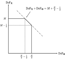
(a) $\frac{N}{2}\geq M-\frac{1}{2}$ and $K\geq M+\frac{N}{2}-\frac{1}{2}$

(b) $M\leq K\leq\frac{N}{2}$ and $K\leq M+\frac{N}{2}-\frac{1}{2}$

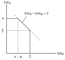
(c) $\frac{N}{2}+\frac{1}{2}\leq M\leq N\leq K$

Figure 3: Examples of DoF region for the multiple access channel without a direct path under different values of $M$, $N$ and $K$.

Theorem 3

Consider the multiple access channel model

$$\mathbf{Y}=\sqrt{P}\mathbf{H}\boldsymbol{\Theta}\mathbf{G}\mathbf{X}+\mathbf{Z},$$ (28)

with $\mathbf{X}$ and $\boldsymbol{\Theta}$ as the two independent inputs, $\mathbf{Y}\in\mathbb{C}^{K}$ as the output, and $\mathbf{Z}\sim\mathcal{CN}(0,\mathbf{I}_{K})$ as the noise. Here, $\mathbf{X}\in\mathbb{C}^{M}$ has a power constraint $\mathbb{E}[\|\mathbf{X}\|_{2}^{2}]\leq 1$, and ${\boldsymbol{{\Theta}}}={\text{diag}}([e^{j\theta_{1}},e^{j\theta_{2}},\cdots,e^{j\theta_{{N}}}])$ has a unit modulus constraint. For almost all matrices $\mathbf{G}\in\mathbb{C}^{N\times M}$ and $\mathbf{H}\in\mathbb{C}^{K\times N}$, the DoF region of the multiple access channel is given by the set of DoF pairs $(\mathrm{DoF}_{\mathbf{X}},\mathrm{DoF}_{\boldsymbol{\Theta}})$ that satisfy

$$\mathrm{DoF}_{\mathbf{X}} \leq \min(M,N,K),$$ (29)

$$\mathrm{DoF}_{\boldsymbol{\Theta}} \leq \min\left(\frac{N}{2},K\right),$$ (30)

$$\mathrm{DoF}_{\mathbf{X}}+\mathrm{DoF}_{\boldsymbol{\Theta}} \leq \min\left(M+\frac{N}{2}-\frac{1}{2},N,K\right).$$ (31)

Proof:

First, we show the converse. The maximum of $\mathrm{DoF}_{\mathbf{X}}$ cannot exceed the DoF of the channel from $\mathbf{X}$ to $\mathbf{Y}$ with $\boldsymbol{\Theta}$ set as a deterministic known constant. In this case, the maximum mutual information between $\mathbf{X}$ and $\mathbf{Y}$ is given by the capacity of a MIMO channel with $\mathbf{H}_{\mathrm{eq}}=\mathbf{H}\boldsymbol{\Theta}\mathbf{G}$ as the equivalent channel. The DoF of this MIMO channel is the rank of the channel matrix, so we have

$$\mathrm{DoF}_{\mathbf{X}}\leq\mathrm{rank}(\mathbf{H}_{\mathrm{eq}})=\min(M,N,K).$$ (32)

An upper bound on $\mathrm{DoF}_{\boldsymbol{\Theta}}$ can be obtained by setting $\mathbf{X}$ to be a constant. In this case, Theorem 2 gives

$$\mathrm{DoF}_{\boldsymbol{\Theta}}\leq\min\left(\frac{N}{2},K\right).$$ (33)

Finally, the sum DoF is upper bounded by allowing cooperation between $\mathbf{X}$ and $\boldsymbol{\Theta}$. By Theorem 1, we have

$$\mathrm{DoF}_{\mathbf{X}}+\mathrm{DoF}_{\boldsymbol{\Theta}}\leq\min\left(M+\frac{N}{2}-\frac{1}{2},N,K\right).$$ (34)

Next, we show achievability. The key is to recognize that the sum DoF as characterized in Theorem 1 is achieved with several choices of independent distributions $p(\mathbf{X})p(\mathbf{\Theta})$. Thus, this same sum DoF is also achievable in the multiple access setting. The different choices of the independent distributions can be used to achieve the different corner points of the DoF region outer bound above.

Choose the distribution of $\mathbf{X}$ and $\boldsymbol{\Theta}$ as in case 2) of Theorem 1, i.e., $\mathbf{X}$ has the phase of its last element fixed, and $\boldsymbol{\Theta}$ is chosen as $\theta_{i}\sim\operatorname{Unif}(-\pi,\pi]$, $\forall i$. We decode $\mathbf{X}$ first, then $\mathbf{\Theta}$, which corresponds to decomposing the sum rate as

$$I(\mathbf{X},\boldsymbol{\Theta};\mathbf{Y})=I\left(\boldsymbol{\Theta};\mathbf{Y}|\mathbf{X}\right)+I(\mathbf{X};\mathbf{Y})$$ (35)

The first term $I\left(\boldsymbol{\Theta};\mathbf{Y}|\mathbf{X}\right)$ gives rise to an achievable $\mathrm{DoF}_{\boldsymbol{\Theta}}$ as (36) below according to Theorem 2. The achievable $\mathrm{DoF}_{\mathbf{X}}$ can be derived by subtracting $\mathrm{DoF}_{\boldsymbol{\Theta}}$ from the achievable sum DoF. This gives the following achievable DoF pair:

$$\mathrm{DoF}_{\boldsymbol{\Theta}}=\min\left(\frac{N}{2},K\right),$$ (36)

$$\mathrm{DoF}_{\mathbf{X}}=\min\left(M+\frac{N}{2}-\frac{1}{2},N,K\right)-\min\left(\frac{N}{2},K\right).$$ (37)

Next, choose the distributions as in case 3) in Theorem 1, which achieves the same sum DoF of $\min\left(M+\frac{N}{2}-\frac{1}{2},N,K\right)$. In this case, $\mathbf{X}$ is i.i.d. complex Gaussian over $M$ elements, i.e., $\mathbf{X}\sim\mathcal{CN}(0,\mathbf{I}_{M})$, and the first $N-1$ elements of $\boldsymbol{\Theta}$ is chosen as uniform distribution with $\theta_{i}\sim\operatorname{Unif}(-\pi,\pi],~{}i=1,\ldots,N-1$, and the last element fixed, i.e., $\theta_{N}=1$. We now decode $\mathbf{\Theta}$ first, then $\mathbf{X}$, which corresponds to decomposing the sum rate as $I(\mathbf{X},\boldsymbol{\Theta};\mathbf{Y})$ as

$$I(\mathbf{X},\boldsymbol{\Theta};\mathbf{Y})=I\left(\mathbf{X};\mathbf{Y}|\boldsymbol{\Theta}\right)+I(\boldsymbol{\Theta};\mathbf{Y})$$ (38)

The first term $I\left(\mathbf{X};\mathbf{Y}|\boldsymbol{\Theta}\right)$ gives rise to an achievable $\mathrm{DoF}_{\mathbf{X}}$ as in (39) below, because the equivalent channel is just a point-to-point MIMO channel with rank $\min(M,N,K)$. The achievable $\mathrm{DoF}_{\boldsymbol{\Theta}}$ can be derived by subtracting $\mathrm{DoF}_{\mathbf{X}}$ from the achievable sum DoF. This gives the following achievable DoF pair:

$$\mathrm{DoF}_{\mathbf{X}}=\min(M,N,K),$$ (39)

$$\mathrm{DoF}_{\boldsymbol{\Theta}}=\min\left(M+\frac{N}{2}-\frac{1}{2},N,K\right)-\min(M,N,K).$$ (40)

Finally by time-sharing, we get the achievability of the entire region (29)-(31). ∎

Depending on the relative values of $M$, $N$ and $K$, the DoF region may take different shapes as shown by several examples in Fig. 3. Case (a) is an example where there is a large number of receive antennas $K$. In this case, the DoF region is constrained by the transmitter dimension $M$ and the RIS dimension $N/2$, but because of the $1/2$ dimension overlap, the DoF region has a pentagon shape. Case (b) is an example where the DoF region is constrained by the receiver dimension $K$. Case (c) is an example where the DoF region is constrained by the RIS dimension $N$. In all three examples, the RIS can transmit additional data streams to the receiver on top of the $M$ data streams from the transmitter. They show the benefit of modulating information through the phases of the RIS.

As an additional remark, the input distributions that achieve the sum DoF in the proof of Theorem 3 are i.i.d. across all the elements of $\mathbf{X}$ and $\boldsymbol{\Theta}$, except the overlapping dimension. This implies that this result can be generalized to the scenarios in which $\mathbf{X}$ or $\boldsymbol{\Theta}$ can consist of multiple users. This corresponds to systems with multiple transmitters or multiple RIS’s.

IV Generalization to RIS System with Direct Path

We now generalize the analysis of the previous section to the channel model where a direct path exists between the transmitter and the receiver. Without the direct path, the previous analysis shows that there is a global phase ambiguity resulting in $1/2$ loss of DoF in both the point-to-point and the multiple access case. In this section, we show that this lost of DoF due to phase ambiguity can be recovered when a direct path is present.

IV-A Joint Transmission with $(\mathbf{X},\mathbf{\Theta})$ as Input

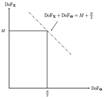
(a) $\frac{N}{2}\geq M$ and $K\geq M+\frac{N}{2}$

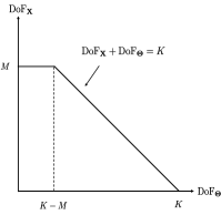
(b) $M\leq K\leq\frac{N}{2}$ and $K\leq M+\frac{N}{2}$

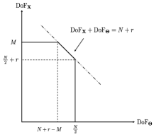
(c) $\frac{N}{2}+r\leq M\leq N+r\leq K$

Figure 4: Examples of DoF region for the multiple access channel with a direct path of rank $r$ under different values of $M$, $N$ and $K$.

The DoF of the point-to-point channel for a channel model with a direct path and with $(\mathbf{X},\mathbf{\Theta})$ as the input and $\mathbf{Y}$ as the output is given by the following theorem.

Theorem 4

Consider the channel model

$$\mathbf{Y}=\sqrt{P}\left(\mathbf{H}{\boldsymbol{\Theta}}\mathbf{G}+\mathbf{F}\right)\mathbf{X}+\mathbf{Z},$$ (41)

with $(\mathbf{X},\boldsymbol{\Theta})$ as the input where $\mathbf{X}\in\mathbb{C}^{M}$ has a power constraint $\mathbb{E}[\|\mathbf{X}\|_{2}^{2}]\leq 1$ and ${\boldsymbol{{\Theta}}}={\text{diag}}([e^{j\theta_{1}},e^{j\theta_{2}},\cdots,e^{j\theta_{{N}}}])$, $\mathbf{Y}\in\mathbb{C}^{K}$ as the output, and $\mathbf{Z}\sim\mathcal{CN}(0,\mathbf{I}_{K})$ as the noise. For almost all $\mathbf{G}$ and $\mathbf{H}$, and almost all direct path channels $\mathbf{F}$ with a fixed rank $r>0$, the maximum DoF from $(\mathbf{X},\boldsymbol{\Theta})$ to $\mathbf{Y}$ is given by

$$\mathrm{DoF}_{(\mathbf{X},\boldsymbol{\Theta})}=\min\left(M+\frac{N}{2},N+r,K\right).$$ (42)

This maximum DoF can be achieved with $\mathbf{X}$ and $\boldsymbol{\Theta}$ being independent.

Proof:

Take the singular-value decomposition (SVD) of the rank-$r$ matrix $\mathbf{F}$

$$\mathbf{F}=\mathbf{U}\boldsymbol{\Sigma}\mathbf{V},$$ (43)

where $\mathbf{U}\in\mathcal{C}^{K\times r}$ and $\mathbf{V}\in\mathcal{C}^{r\times M}$ are unitary matrices, and $\boldsymbol{\Sigma}$ is a diagonal matrix of dimension $r$ with positive entries $\sigma_{1},\ldots,\sigma_{r}$. We rewrite the channel model as

$$\mathbf{Y} =\sqrt{P}\left(\mathbf{H}{\boldsymbol{\Theta}}\mathbf{G}+\mathbf{F}\right)\mathbf{X}+\mathbf{Z},$$ (44)

$$=\sqrt{P}\left(\mathbf{H}{\boldsymbol{\Theta}}\mathbf{G}+\mathbf{U}\boldsymbol{\Sigma}\mathbf{V}\right)\mathbf{X}+\mathbf{Z},$$ (45)

$$=\sqrt{P}[\mathbf{H},\mathbf{U}\boldsymbol{\Sigma}]\left[\begin{array}[]{cc}{\boldsymbol{\Theta}}&\mathbf{0}\\ \mathbf{0}&\mathbf{I}_{r}\\ \end{array}\right]\left[\begin{array}[]{c}\mathbf{G}\\ \mathbf{V}\\ \end{array}\right]\mathbf{X}+\mathbf{Z},$$ (50)

$$=\sqrt{P}\mathbf{H^{\prime}}\underbrace{{\boldsymbol{\Theta}^{\prime}}\mathbf{G^{\prime}}\mathbf{X}}_{\mathbf{W^{\prime}}}+\mathbf{Z},$$ (51)

where $\mathbf{H^{\prime}}=[\mathbf{H},\mathbf{U}\boldsymbol{\Sigma}]$, $\boldsymbol{\Theta^{\prime}}=\left[\begin{array}[]{cc}{\boldsymbol{\Theta}}&\mathbf{0}\\ \mathbf{0}&\mathbf{I}_{r}\\ \end{array}\right]$ and $\mathbf{G^{\prime}}=\left[\begin{array}[]{c}\mathbf{G}\\ \mathbf{V}\\ \end{array}\right]$. The channel model (51) is now a model without a direct path and with an RIS of effective size $N^{\prime}=N+r$. The intuition behind this reformulation is that the direct path channel can be regarded as a separate RIS with $r$ elements where the phase shifts are fixed at $0$ (or any arbitrary known phase).

Consider first the case with $r=1$. The overall system can now be viewed as a channel with an RIS of $N^{\prime}=N+1$ reflective elements, but without a direct path. We choose the input distribution as $\mathbf{X}$ to be i.i.d. complex Gaussian for the $M$ elements, i.e., $\mathbf{X}\sim\mathcal{CN}(0,\mathbf{I}_{M})$, and the first $N$ elements of $\boldsymbol{\Theta^{\prime}}$ to follow uniform distribution with $\theta_{i}\sim\operatorname{Unif}[-\pi,\pi),~{}i=1,\ldots,N$. The last element of $\boldsymbol{\Theta^{\prime}}$ is set to be fixed at $1$. This choice of distribution is exactly the distributions in case 2) of Theorem 1. From Theorem 1, we see that the DoF achieved by this distribution for a system of size $(M,N^{\prime},K)$ is given as

$$\min\left(M+\frac{N^{\prime}}{2}-\frac{1}{2},N^{\prime},K\right)=\min\left(M+\frac{N}{2},N+1,K\right).$$ (52)

This proves the result for the case of $r=1$.

For the case of $r>1$, we need to make use of the techniques in the proof of Theorem 1 involving characterizing the information dimension $D(\mathbf{W}^{\prime})$ and its behavior under projection. The details are in Appendix C. ∎

Theorem 4 shows that a direct path between the transmitter and the receiver helps resolve the global phase ambiguity and recover the $1/2$ DoF loss. Moreover, this can already be achieved with a direct path of channel rank of just $1$.

IV-B Multiple Access Channel with $\mathbf{X}$ and $\mathbf{\Theta}$ as Inputs

In this section, we consider the scenario in which the transmitter and the RIS send independent messages to the receiver. Similar to the case without the direct path, since the distribution that achieves the maximum DoF in the joint transmission as given in Theorem 4 is already in the form of a product of two independent distributions, this gives the following characterization of the DoF region of the multiple access channel with a direct path between the transmitter and the receiver.

Theorem 5

Consider the multiple access channel model

$$\mathbf{Y}=\sqrt{P}\left(\mathbf{H}{\boldsymbol{\Theta}}\mathbf{G}+\mathbf{F}\right)\mathbf{X}+\mathbf{Z},$$ (53)

with $\mathbf{X}$ and $\boldsymbol{\Theta}$ as the two independent inputs, $\mathbf{Y}\in\mathbb{C}^{K}$ as the output, and $\mathbf{Z}\sim\mathcal{CN}(0,\mathbf{I}_{K})$ as the noise. Here $\mathbf{X}\in\mathbb{C}^{M}$ has a power constraint $\mathbb{E}[\|\mathbf{X}\|_{2}^{2}]\leq 1$ and ${\boldsymbol{{\Theta}}}={\text{diag}}([e^{j\theta_{1}},e^{j\theta_{2}},\cdots,e^{j\theta_{{N}}}])$. For almost all $\mathbf{G}$ and $\mathbf{H}$, and almost all direct path channel $\mathbf{F}$ with a fixed rank $r>0$, the DoF region of the multiple access channel is given by the set of DoF pairs ($\mathrm{DoF}_{\mathbf{X}}$,$\mathrm{DoF}_{\boldsymbol{\Theta}}$) that satisfy

$$\mathrm{DoF}_{\mathbf{X}} \leq \min(M,N+r,K),$$ (54)

$$\mathrm{DoF}_{\boldsymbol{\Theta}} \leq \min\left(\frac{N}{2},K\right),$$ (55)

$$\mathrm{DoF}_{\mathbf{X}}+\mathrm{DoF}_{\boldsymbol{\Theta}} \leq \min\left(M+\frac{N}{2},N+r,K\right).$$ (56)

Proof:

First, we show the converse. The maximum $\mathrm{DoF}_{\mathbf{X}}$ cannot exceed the DoF of the channel from $\mathbf{X}$ to $\mathbf{Y}$ with $\boldsymbol{\Theta}$ set as a deterministic known constant. In this case, the maximum mutual information between $\mathbf{X}$ and $\mathbf{Y}$ is given by the capacity of a MIMO channel with $\mathbf{H}_{\mathrm{eq}}=\mathbf{H}\boldsymbol{\Theta}\mathbf{G}+\mathbf{F}$ as the equivalent channel. The DoF of this MIMO channel is the rank of the equivalent channel, which gives (54).

An upper bound on $\mathrm{DoF}_{\boldsymbol{\Theta}}$ can be obtained by setting $\mathbf{X}$ to be a deterministic known constant. In this case, Theorem 2 gives (55). Finally, the sum DoF is upper bounded by allowing cooperation between $\mathbf{X}$ and $\boldsymbol{\Theta}$. By Theorem 4, we have (56).

Next, we show achievability. Recognizing that the sum DoF as characterized in Theorem 4 is achieved with an independent distribution $p(\mathbf{X})p(\mathbf{\Theta})$, it must also be an achievable sum DoF in the multiple access setting. By choosing to decode $\mathbf{X}$ first, then $\mathbf{\Theta}$, we get the following achievable DoF pair corresponding to one corner point of the DoF region outer bound:

$$\mathrm{DoF}_{\boldsymbol{\Theta}}=\min\left(\frac{N}{2},K\right),$$ (57)

$$\mathrm{DoF}_{\mathbf{X}}=\min\left(M+\frac{N}{2},N+r,K\right)-\min\left(\frac{N}{2},K\right).$$ (58)

The opposite decoding order achieves the other corner point. This shows that the entire region (54)-(56) is achievable. ∎

As the case without the direct path, depending on the relative values of $M$, $N$ and $K$, the DoF region can take different shapes as shown by three examples in Fig. 4. In all three examples, modulating information through RIS allows additional data streams to be transmitted to the receiver. The effect of the direct path is evidence in cases (a), where the direct path helps resolve the phase ambiguity hence removing the $1/2$ dimension overlap, and in (c), where the sum DoF is improved by the rank of the direct path.

V Modulating Information Through Phases

The DoF analysis of the previous sections gives theoretic results on how many independent data streams can be transmitted through the phases of an RIS system. In this section we suggest two different ways of modulating information through the phases of the RIS.

First, we describe a maximum likelihood (ML) decoding strategy to jointly decode the modulated information in $\mathbf{X}$ and $\boldsymbol{\Theta}$. Second, we propose a symbol-level precoding scheme to jointly encode information in $\mathbf{X}$ and $\boldsymbol{\Theta}$.

V-A Maximum Likelihood Decoding

A straightforward way to modulate information jointly through the transmitter and the phases of the RIS is to use fixed constellations to encode the information at $\mathbf{X}$ and $\boldsymbol{\Theta}$, then use maximum likelihood (ML) decoding to jointly decode the transmitted symbols. Due to the phase-only nature of RIS, PSK constellation can be used at $\boldsymbol{\Theta}$. The encoding at $\mathbf{X}$ can be in the form of symbols from constellation points multiplied by a fixed precoding vector (or precoding matrix in case of multiple data streams). Assuming the general case of an RIS system with a direct path, the ML estimate of the transmitted symbols at the decoder is given by:

$$({\mathbf{\hat{X}}},{\boldsymbol{\hat{\Theta}}})=\mathrm{argmin}_{(\mathbf{X},\boldsymbol{\Theta})\in{\mathcal{C}}}{\|\mathbf{Y}-\sqrt{P}(\mathbf{H}\boldsymbol{\Theta}\mathbf{G}+\mathbf{F})\mathbf{X}\|^{2}}.$$ (59)

where the minimization is over the constellations of $\mathbf{X}$ and $\boldsymbol{\Theta}$, denoted as $\mathcal{C}$ in the above. This is a discrete optimization problem for which finding a global optimal solution would have a high computational complexity. This approach of modulating information in the phase shifts at RIS has been explored in [20] and [21] by solving problem (59) using approximation algorithms.

V-B Symbol-Level Precoding

As an alternative to encoding information using fixed constellations at the transmitter $\mathbf{X}$ and the RIS $\boldsymbol{\Theta}$, in this section we propose a symbol-level precoding strategy that sets the received signal $\mathbf{Y}$ to be as close to the desired points in a fixed constellation as possible. The idea is to try to directly make $\mathbf{Y}$ to be the symbols corresponding to the information to be transmitted, and to design $\mathbf{X}$ and $\boldsymbol{\Theta}$ so that the desired symbols are synthesized at the receiver. Because $\mathbf{X}$ and $\boldsymbol{\Theta}$ are jointly designed, this strategy is applicable to the joint transmission case, but not to the multiple access setting.

In the below, we discuss the symbol-level precoding problem formulation and the numerical algorithms for solving the precoding problem.

V-B1 Problem Formulation

Given a vector ${\mathbf{\hat{Y}}}$ corresponding to the desired constellation points at the receiver and assuming perfect CSI, symbol-level precoding proceeds by solving the following optimization problem:

$$({\mathbf{X^{*}}},{\boldsymbol{\Theta^{*}}})=\mathrm{argmin}_{\mathbf{X},\boldsymbol{\Theta}}{\|\hat{\mathbf{Y}}-\sqrt{P}\left(\mathbf{H}\boldsymbol{\Theta}\mathbf{G}+\mathbf{F}\right)\mathbf{X}\|^{2}}.$$ (60)

subject to that $\|\mathbf{X}\|^{2}_{2}\leq 1$ and $\boldsymbol{\Theta}={\rm diag}([e^{j\theta_{1}},\cdots,e^{j\theta_{N}})$. A special case of this is when the transmit signal $\mathbf{X}$ is deterministic as studied in Section III-C, for which the optimization problem can be formulated as:

$${\boldsymbol{\Phi^{*}}}=\mathrm{argmin}_{\boldsymbol{\Phi}}\|\bar{\mathbf{Y}}-\sqrt{P}\bar{\mathbf{H}}\mathbf{\Phi}\|^{2},$$ (61)

where $\boldsymbol{\Phi}=[e^{j\theta_{1}},\ldots,e^{j\theta_{N}}]^{T}$ is the vector form of the diagonal matrix $\boldsymbol{\Theta}$, $\bar{\mathbf{H}}=\mathbf{H}\mathrm{diag}(\mathbf{G}\mathbf{X})$ is the equivalent channel, and $\bar{\mathbf{Y}}=\mathbf{\hat{Y}}-\mathbf{FX}$ is the effective received signal. This special case has the same formulation as the problem of MIMO precoding with per-antenna constant envelope constraints, as studied in [28, 29].

If the above optimization problem can be solved to achieve a (near)-zero minimum, the resulting (${\mathbf{X^{*}}},{\boldsymbol{\Theta^{*}}}$) can be directly used as the transmit signal and the reflective coefficients, in which case the desired constellation points plus noise would be received at $\mathbf{Y}$.

This symbol-level precoding strategy has been proposed earlier for MIMO channels in various formulations [30, 31]. In this paper, we apply the concept to the RIS system. Moreover, we point out that it is possible to numerically evaluate the relationships between the dimensions of $\mathbf{X}$, $\mathbf{\Theta}$ and $\mathbf{Y}$ that allow this optimization problem to be solved to a near-zero minimum. This gives a method to numerically characterize the achievable DoF of the RIS system.

V-B2 Numerical Algorithm

A main advantage of the symbol-level precoding formulation is that instead of solving a discrete optimization problem (59), we now solve a continuous optimization problem (60). Although (60) is not convex, as it involves product of optimization variables in a bilinear form as the objective and unit modulus constraints, there are optimization techniques available that allow efficient gradient search to find local optimal solutions.

Specifically, this paper uses an approach based on the augmented Lagrangian approach [32] to take care of the power constraint on $\mathbf{X}$ and a Riemannian conjugate gradient method [33] to account for the unit modulus constraint on $\boldsymbol{\Theta}$ to solve (60). The Riemannian conjugate gradient method recognizes the fact that the unit modulus constraints force $\mathbf{\Theta}$ to be on a complex circle manifold, and modifies the traditional gradient descent algorithm (which works on the Euclidean space) to work on the manifold to enhance the convergence speed. A description of the numerical method for solving the optimization problems (60) is given in Appendix D. This algorithm is used in the next section to numerically verify the DoF analysis for modulating information through the phases of the RIS.

VI Numerical Results

In this section we present numerical results based on the symbol-level precoding approach to validate the DoF analysis of jointly modulating information by the transmitter and the RIS for the receiver.

VI-A Channel Model and Simulation Setting

We consider a MIMO communication system with an RIS, consisting of a transmitter with $2$ antennas and a receiver with 4 antennas. The number of elements of the RIS varies in different simulation settings. All the channel entries follow i.i.d. Rayleigh fading with unit variance, i.e., $\mathcal{CN}(0,1)$.

The idea is to perform symbol-level precoding to synthesize the desired constellation point $\mathbf{Y}$ by solving for $\mathbf{X}$ and $\boldsymbol{\Theta}$ in (60) or (61). We use the Riemannian conjugate gradient approach to find a local optimal solution, and consider a point to be feasible if the synthesized point is within a distance threshold of $\delta=10^{-3}$ from the desired point.

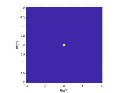
(a) $N=4$

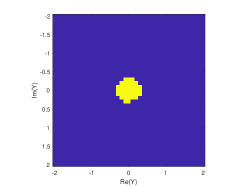
(b) $N=5$

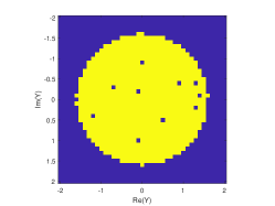
(c) $N=6$

Figure 5: The feasible region of $y$ for synthesizing $\mathbf{Y}=[y,y,y,y]$ at $M=2$, $K=4$, $P=1$, and $N$ ranging from 4 to 6 for channels without the direct path. Color yellow means that a point is feasible while color blue means that a point is infeasible.

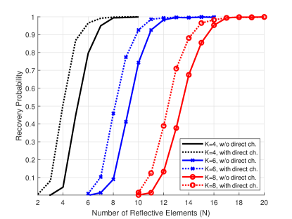
Figure 6: Probability of successfully synthesizing $\mathbf{Y}$ at the receiver with each component of $\mathbf{Y}$ a random point on the unit circle for different values of $N$, with $M=2$ and $P=10$.

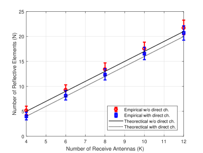
Figure 7: The number of RIS elements $N$ needed to successfully synthesize a $K$-dimensional $\mathbf{Y}$ with each element of $\mathbf{Y}$ being a random point on the complex unit circle. The theoretical lines correspond to the DoF results in Theorems 1 and 4, i.e., $N=2K-2M$ and $N=2K-2M+1$ for the case with and without the direct path, respectively. The error bars of the empirical points correspond to 80, 50, and 20-percentile probabilities of success for synthesizing $\mathbf{Y}$.

VI-B Dimension of the Symbol-Level Precoded Signal

The DoF of joint transmission through the transmitter and the RIS can be numerically verified by visualizing the dimension of the set of feasible receive points $\mathbf{Y}$. For example, in the case with no direct path, assuming that $M+\frac{N}{2}-\frac{1}{2}\geq K$, the set of points that $\mathbf{H\Theta G}\mathbf{X}$ can reach should form a $K$-dimensional set in the complex space. In other words, for each element of $\mathbf{Y}$, the set of reachable points by designing $\mathbf{X}$ and $\boldsymbol{\Theta}$ should be a two-dimensional set in the real and imaginary plane.

Fig. 5 shows an example of this phenomenon with $M=2$, $K=4$ and $N$ varying from $4$ to $6$ for the case of without the direct path. The transmit power $P$ is set to be $1$. The feasible regions for $y$ with $\mathbf{Y}=[y,y,y,y]^{T}$ are shown with color marked to represent the feasibility of the points. Yellow means that a point is feasible; blue means that a point is infeasible. A first observation is that increasing the effective transmit dimension $M+\frac{N}{2}-\frac{1}{2}$ enlarges the feasible region. At $N=4$, no points are feasible except the origin. When $N=5$, the feasible region becomes a two-dimensional region in each component of $\mathbf{Y}$. At $N=6$, the feasibility region is further enlarged. This agrees with the theoretical analysis that $N=5$ is needed to achieve a DoF of $4$.

VI-C Phase Transition for Reaching the Desired Points

To further illustrate the phase transition from the infeasibility to feasibility, we plot the probability of reaching a desired point in Fig. 6. We choose $y_{1},\ldots,y_{K}$ to be random points on the complex unit circle and aim to synthesize $\mathbf{Y}=[y_{1},\ldots,y_{K}]^{T}$ as the desired point. We increase the transmit power to $P=10$ in order to make the desired points to be in the feasible region (should the region exist). This is to avoid the situation in which the infeasibility is due to the transmit power being too low.

Fig. 6 shows the probability of successful synthesis against the number of elements at the RIS. It illustrates the phase transition with respect to $N$. The number of transmit antennas is $M=2$. The cases for $K=4,~{}6,~{}8$ are plotted in the same scale. Each plot is generated by solving (60) for the scenarios with or without the direct path, respectively, over 1000 channel realizations. From Fig. 6, we observe that the phase transition have the median at around $N=2K-2M+1$ for the case of without the direct path, and $N=2K-2M$ with the direct path, which verifies the DoF results. Further, there is a gap of $1$ RIS element between the two cases, which correspond to the $1/2$ dimension difference in the DoF result. This matches Theorem 1 and Theorem 5.

To further illustrate the phase transition, Fig. 7 shows the number of RIS elements corresponding to the $20$, $50$ and $80$ percentile probabilities of successfully synthesizing a received vector $\mathbf{Y}$ with $K$ antennas. The theoretical DoF curves of $N=2K-2M$ and $N=2K-2M+1$ are also plotted, for the scenarios with and without the direct path, respectively. From Fig. 7, we observe that the theoretical DoF curves are slightly below the $50$-percentile points. The gap between the $80$-percentile points and the theoretical DoF curves is about $1$ to $2$ RIS elements, and the gap between the $20$-percentile points and the theoretical DoF curves is about $0$ to $1$ RIS element. These results verify the theoretical analysis. It also shows that to ensure consistent feasibility of synthesizing a received vector, it is important to have slightly more than the minimum number of RIS elements.

VII Conclusions

This paper studies the information theoretic limits of joint information transmission using both the RF input and phase modulation at an RIS reflector. In particular, the DoF or the multiplex gain of the communication schemes where information is conveyed through the RF transmitted symbols and the reflective coefficients of the RIS is characterized for both the point-to-point and the multiple access settings. This proposed use of the RIS significantly improves the DoF of the overall system as compared to the conventional paradigm of simply using the RIS as a passive beamformer for enhancing the channel strength.

The theoretical DoF analysis in this paper is obtained by recognizing a connection between the RIS channel and the MIMO channels with phase noises. Tools for studying the information dimension and the point-wise dimension under projection are used to obtain the DoF result. For example, as compared to a MIMO channel with $M$ transmit antennas and $K$ receive antennas, which has a DoF of $\min(M,K)$, an RIS system with the same number of transmit and receive antennas and further equipped with a reconfigurable surface of $N$ reflective elements can achieve an overall DoF of $\min(M+\frac{N}{2}-\frac{1}{2},N,K)$ by allowing joint encoding by the transmitter and the RIS, (assuming no direct path between the transmitter and the receiver). This shows the significant potential of using the RIS to modulate information and to improve the overall transmission rate in a system limited by the number of transmit antennas.

Finally, this paper proposes a symbol-level precoding strategy to enable the practical realization of modulating information through the phases of the RIS. We show numerically that the phase transition for successful symbol-level precoding agrees with the theoretical DoF analysis.

Appendix A Information Dimension Under Project and
Proof of Theorem 1

We present the proof of Theorem 1 by first building a connection between the model (4) and the MIMO channel model with phase noise. Then, we make use of the concepts of information dimension and point-wise dimension, and study their behavior under projections, to compute the DoF of (4).

A-A Information Dimension and DoF

Definition 1

For a random vector $\mathbf{X}\in\mathbb{R}^{N}$ with distribution $\mu$, we define the information dimension of $\mathbf{X}$ as

$${D}(\mathbf{X})=\lim_{\varepsilon\to 0}\frac{\mathbb{E}\left[\log\mu\left(B(\mathbf{X};\varepsilon)\right)\right]}{\log\varepsilon}$$ (62)

assuming that the limit exists, where $B(\mathbf{X};\varepsilon)\subseteq\mathbb{R}^{N}$ denotes the ball with center $\mathbf{X}$ and radius $\varepsilon$ with respect to an arbitrary norm on $\mathbb{R}^{N}$.

The following lemma connects the concept of information dimension to the multiplexing gain of a general vector additive noise channel.

Lemma 1 ([34],[35])

Let $\mathbf{X}$ and $\mathbf{Z}$ be independent random vectors in $\mathbb{R}^{n}$ such that $\mathbf{Z}$ has an absolutely continuous distribution with $h(\mathbf{Z})>-\infty$ and $H(\lfloor\mathbf{Z}\rfloor)<\infty$. Then

$$\limsup_{P\to\infty}\frac{I(\mathbf{X};\sqrt{P}\mathbf{X}+\mathbf{Z})}{\frac{1}{2}\log P}=D(\mathbf{X}).$$ (63)

By Lemma 1, we see that computing the multiplexing gain of the RIS channel (4) can be equivalently cast as computing the information dimension $D(\mathbf{H}\boldsymbol{\Theta}\mathbf{GX})$. However, Lemma 1 deals with real channels. To work with a complex channel model, we can stack the real and imaginary parts of the complex vectors, and stack the real and imaginary parts of complex matrices, such as $\mathbf{H}$, as

$$\left[\begin{array}[]{cc}\Re\{\mathbf{H}\}&-\Im\{\mathbf{H}\}\\ \Im\{\mathbf{H}\}&\Re\{\mathbf{H}\}\\ \end{array}\right],$$ (66)

then apply Lemma 1 to the resulting equivalent model in $\mathbb{R}^{2K}$. Note that two real dimensions in $\mathbb{R}^{2K}$ is equivalent to one complex dimension in $\mathbb{C}^{K}$.

A-B Information Dimension of $\mathbf{W}$ via a Connection to the MIMO Phase Noise Channel

In this section, we compute the information dimension of the output of the RIS $\mathbf{W}$ in (4). First, consider the following channel model (with general arbitrary dimensions):

$$\mathbf{\tilde{Y}}=\sqrt{P}{\boldsymbol{\tilde{\Theta}}}\mathbf{\tilde{G}}\mathbf{\tilde{X}}+\mathbf{\tilde{Z}},$$ (67)

where $\mathbf{\tilde{Y}}\in\mathbb{C}^{\tilde{N}}$, $\mathbf{\tilde{X}}\in\mathbb{C}^{\tilde{M}}$, ${\boldsymbol{\tilde{\Theta}}}={\text{diag}}([e^{j\theta_{1}},e^{j\theta_{2}},\cdots,e^{j\theta_{\tilde{N}}}])$. A crucial observation is that this channel model resembles the MIMO channel with phase noise. We leverage the following result from the phase noise literature for a key insight.

Lemma 2 ([36])

Let $\boldsymbol{\tilde{\Phi}}=[e^{j\theta_{1}},\ldots,e^{j\theta_{\tilde{N}}}]^{T}$ be a vector of random phases such that $h(\boldsymbol{\tilde{\Phi}})>-\infty$ and

$$\bar{\mathbf{Y}}=\sqrt{P}{\boldsymbol{\tilde{\Phi}}}\circ\left(\mathbf{\tilde{G}}\mathbf{\tilde{X}}\right)+\mathbf{\tilde{Z}},$$ (68)

where $\circ$ denotes element-wise product and $\mathbf{\tilde{Z}}\sim\mathcal{CN}(0,\mathbf{I}_{\tilde{N}})$. For $\mathbf{\tilde{X}}\sim\mathcal{CN}(0,\mathbf{I}_{\tilde{M}})$, we have that

$$h(\bar{\mathbf{Y}})\geq\min\left(\tilde{M}+\frac{\tilde{N}}{2}-\frac{1}{2},\tilde{N}\right)\log^{+}P+c_{1}.$$ (69)

Further, for any distribution of $\mathbf{X}$, we have

$$I(\bar{\mathbf{Y}};\mathbf{\tilde{X}})\leq\min\left(\tilde{M}-\frac{1}{2},\frac{\tilde{N}}{2}\right)\log^{+}P+c_{2}$$ (70)

Here $c_{1}$ and $c_{2}$ are constants that do not depend on $P$.

The intuition behind (69) is the following. The information dimension of the entropy term $h(\bar{\mathbf{Y}})$ is clearly lower bounded by the dimension of $\mathbf{\bar{Y}}$ which is $\tilde{N}$, but it is also lower bounded by the transmit dimension, which is the sum of $\tilde{M}$ and $\tilde{N}/2$ but subtracting $1/2$. Here, $\tilde{M}$ is the information dimension of $\mathbf{\tilde{X}}$; $\tilde{N}/2$ is the information dimension of the phases $\mathbf{\tilde{\Phi}}$; but, because there is a common phase between them as the two are multiplied, we need to subtract the dimension of their overlap, which is $1/2$.

We are now ready to characterize the information dimension of $\mathbf{W}$ in (4). The result below is for arbitrary dimensions $\tilde{N}$ and $\tilde{M}$.

Lemma 3

Consider the channel model

$$\mathbf{\tilde{Y}}=\sqrt{P}\mathbf{\tilde{W}}+\mathbf{\tilde{Z}}=\sqrt{P}{\boldsymbol{\tilde{\Theta}}}\mathbf{\tilde{G}}\mathbf{\tilde{X}}+\mathbf{\tilde{Z}},$$ (71)

where $\mathbf{\tilde{Y}}\in\mathbb{C}^{\tilde{N}}$ is the output, $\mathbf{\tilde{X}}\in\mathbb{C}^{\tilde{M}}$ with power constraint $\mathbb{E}[\|\mathbf{\tilde{X}}\|_{2}^{2}]\leq 1$ and ${\boldsymbol{\tilde{\Theta}}}={\text{diag}}([e^{j\theta_{1}},e^{j\theta_{2}},\cdots,e^{j\theta_{\tilde{N}}}])$ are the inputs, and $\mathbf{\tilde{Z}}\sim\mathcal{CN}(0,\mathbf{I}_{\tilde{N}})$ is the noise. For almost all matrices $\mathbf{\tilde{G}}\in\mathbb{C}^{\tilde{N}\times\tilde{M}}$, the maximum DoF of $I(\mathbf{\tilde{X}},\boldsymbol{\tilde{\Theta}};\mathbf{\tilde{Y}})$ is given by $\min(\tilde{M}+\frac{\tilde{N}}{2}-\frac{1}{2},\tilde{N})$. This DoF can be achieved using any of the following choices of distributions for $\mathbf{\tilde{X}^{\prime}}$ and $\boldsymbol{\tilde{\Theta}^{\prime}}$.

1. $\mathbf{\tilde{X}}\sim\mathcal{CN}(0,\mathbf{I}_{\tilde{M}})$ and $\boldsymbol{\tilde{\Theta}}$ with $\theta_{i}\sim\operatorname{Unif}(-\pi,\pi]$

2. The distribution of $\mathbf{\tilde{X}}$ is chosen such that the first $\tilde{M}-1$ elements are i.i.d. complex Gaussian, i.e., $\mathbf{\tilde{X}}_{\tilde{M}-1}\sim\mathcal{CN}(0,\mathbf{I}_{\tilde{M}-1})$, and $\tilde{X}_{\tilde{M}}$ is chosen to be real with a chi-squared distribution with 2 degrees of freedom, and $\boldsymbol{\tilde{\Theta}}$ remains as $\tilde{\theta}_{i}\sim\operatorname{Unif}(-\pi,\pi]$.

3. The distribution of $\mathbf{\tilde{X}}$ is i.i.d. complex Gaussian for all $\tilde{M}$ elements, i.e., $\mathbf{\tilde{X}}\sim\mathcal{CN}(0,\mathbf{I}_{\tilde{M}})$, and the first $\tilde{N}-1$ elements of $\boldsymbol{\tilde{\Theta}}$ is chosen as uniform distribution with $\tilde{\theta}_{i}\sim\operatorname{Unif}(-\pi,\pi],~{}i=1,\ldots,N-1$, and the last element of $\boldsymbol{\tilde{\Theta}}$ is fixed as 1, i.e., $\tilde{\theta}_{N}=1$.

With any of these three choices of distributions, the information dimension of $\mathbf{\tilde{W}}$ is

$$D(\mathbf{\tilde{W}})=\min\left(\tilde{M}+\frac{\tilde{N}}{2}-\frac{1}{2},\tilde{N}\right).$$ (72)

Proof:

We show the achievability of the DoF by making use of Lemma 2. Observe that with $\boldsymbol{\tilde{\Phi}}=[e^{j\theta_{1}},\ldots,e^{j\theta_{\tilde{N}}}]^{T}$, we have

$$\mathbf{\tilde{Y}} =\sqrt{P}{\boldsymbol{\tilde{\Theta}}}\mathbf{\tilde{G}}\mathbf{\tilde{X}}+\mathbf{\tilde{Z}}$$ (73)

$$=\sqrt{P}{\boldsymbol{\tilde{\Phi}}}\circ(\mathbf{\tilde{G}}\mathbf{\tilde{X}})+\mathbf{\tilde{Z}}.$$ (74)

Therefore, the RIS channel model in (71) can be viewed as a channel with phase shifts $\boldsymbol{\tilde{\Phi}}$ applied at the receiver. Choosing $\mathbf{\tilde{X}}\sim\mathcal{CN}(0,\mathbf{I}_{\tilde{M}})$ and $\boldsymbol{\tilde{\Phi}}$ as $\theta_{i}\sim\operatorname{Unif}(-\pi,\pi]$, we have that $h(\boldsymbol{\tilde{\Phi}})>-\infty$, therefore we can apply (69) in Lemma 2 to get $h(\mathbf{\tilde{Y}})\geq\min(\tilde{M}+\frac{\tilde{N}}{2}-\frac{1}{2},\tilde{N})\log^{+}P+c_{1}$. The achievability of the desired DoF now follows by lower bounding the mutual information as follows:

$$I(\mathbf{\tilde{X}},\boldsymbol{\tilde{\Theta}};\mathbf{\tilde{Y}}) =h(\mathbf{\tilde{Y}})-h(\mathbf{\tilde{Y}}|\mathbf{\tilde{X}},\boldsymbol{\tilde{\Theta}})$$ (75)

$$\geq\min\left(\tilde{M}+\frac{\tilde{N}}{2}-\frac{1}{2},\tilde{N}\right)\log^{+}P+c_{1},$$ (76)

where the inequality comes from the fact that $h(\mathbf{\tilde{Y}}|\mathbf{\tilde{X}},\boldsymbol{\tilde{\Theta}})$ is the entropy of the noise term which does not depend on $P$.

Next, we prove the converse by giving an upper bound on $I(\mathbf{\tilde{X}},\boldsymbol{\tilde{\Theta}};\mathbf{\tilde{Y}})$. First, for $\boldsymbol{\tilde{\Theta}}$ such that $h(\boldsymbol{\tilde{\Theta}})>-\infty$

$$I\left(\mathbf{\tilde{X}},\boldsymbol{\tilde{\Theta}};\mathbf{\tilde{Y}}\right)=I(\mathbf{\tilde{X}};\mathbf{\tilde{Y}})+I(\boldsymbol{\tilde{\Theta}};\mathbf{\tilde{Y}}|\mathbf{\tilde{X}})$$ (77)

$$\leq\min\left(\tilde{M}-\frac{1}{2},\frac{\tilde{N}}{2}\right)\log^{+}P+I\left(\boldsymbol{\tilde{\Theta}};\mathbf{\tilde{Y}}|\mathbf{\tilde{X}}\right)+c_{2},$$ (78)

where the inequality follows from applying (70) in Lemma 2. To upper bound $I\left(\boldsymbol{\tilde{\Theta}};\mathbf{\tilde{Y}}|\mathbf{\tilde{X}}\right)$, note that when $\mathbf{\tilde{X}}$ is known,

$$\mathbf{\tilde{Y}} =\sqrt{P}\boldsymbol{\tilde{\Theta}}\mathbf{\tilde{G}}\mathbf{\tilde{X}}+\mathbf{\tilde{Z}}$$ (79)

$$=\sqrt{P}\mathrm{diag}(\mathbf{\tilde{G}}\mathbf{\tilde{X}})\boldsymbol{\tilde{\Phi}}+\mathbf{Z},$$ (80)

where $\boldsymbol{\tilde{\Phi}}=[e^{j\theta_{1}},\ldots,e^{j\theta_{\tilde{N}}}]^{T}$. Thus, (79) is equivalent to a MIMO channel with continuous phase inputs on each of the transmit antennas, so

$$I\left(\boldsymbol{\tilde{\Theta}};\mathbf{\tilde{Y}}|\mathbf{\tilde{X}}\right) =I(\boldsymbol{\tilde{\Phi}};\mathrm{diag}(\mathbf{\tilde{G}}\mathbf{\tilde{X}})\boldsymbol{\tilde{\Phi}}+\mathbf{\tilde{Z}}|\mathbf{\tilde{X}})$$ (81)

$$=\sum_{i=1}^{\tilde{N}}I\left(\theta_{i};\sqrt{P}(\mathbf{\tilde{G}}\mathbf{\tilde{X}})_{i}e^{j\theta_{i}}+\tilde{Z}_{i}|\mathbf{\tilde{X}}\right)$$ (82)

$$\leq\frac{\tilde{N}}{2}\log^{+}P+c.$$ (83)

where the last equality follows from applying capacity results for phase-only transmission in single-antenna channels [26] and $c$ is a constant that does not depend $P$. Now we have

$$I\left(\mathbf{\tilde{X}},\boldsymbol{\tilde{\Theta}};\mathbf{\tilde{Y}}\right) \leq\min\left(\tilde{M}-\frac{1}{2},\frac{\tilde{N}}{2}\right)\log^{+}P$$

$$\qquad\qquad+\frac{\tilde{N}}{2}\log^{+}P+c$$ (84)

$$=\min\left(\tilde{M}+\frac{\tilde{N}}{2}-\frac{1}{2},\tilde{N}\right)\log^{+}P+c.$$ (85)

It is not hard to see that the above still holds even when $h(\boldsymbol{\tilde{\Theta}})=-\infty$. This is because even if some $\theta_{i}$ is discrete, the $\min(\tilde{M}-\frac{1}{2},\frac{\tilde{N}}{2})$ term in (84) due to the information dimension of $\mathbf{\tilde{X}}$ would increase by at most $\frac{1}{2}$, while the $\frac{\tilde{N}}{2}$ term due to the information dimension of $\mathbf{\tilde{\Theta}}$ would decrease by at least $\frac{1}{2}$.

Combining (76) and (85), we see that the maximum DoF of the channel model (71) is given by $\min(\tilde{M}+\frac{\tilde{N}}{2}-\frac{1}{2},\tilde{N})$. The information dimension of $\mathbf{\tilde{W}}=\boldsymbol{\tilde{\Theta}}\mathbf{\tilde{G}\tilde{X}}$ is therefore given by $D(\mathbf{\tilde{W}})=\min(\tilde{M}+\frac{\tilde{N}}{2}-\frac{1}{2},\tilde{N})$ in view of Lemma 1.

The proof so far has used the distribution in case 1) in the lemma statement, i.e., $\mathbf{\tilde{X}}\sim\mathcal{CN}(0,\mathbf{I}_{\tilde{M}})$ and $\boldsymbol{\tilde{\Theta}}$ with $\tilde{\theta}_{i}\sim\operatorname{Unif}(-\pi,\pi]$ to achieve the information dimension of $\mathbf{\tilde{W}}=\boldsymbol{\tilde{\Theta}}\mathbf{\tilde{G}\tilde{X}}$ as $\min(\tilde{M}+\frac{\tilde{N}}{2}-\frac{1}{2},\tilde{N})$. Denote the phase of the last element of $\mathbf{\tilde{X}}$ as $e^{j\phi}$, and the phase of the last element of $\tilde{\boldsymbol{\Theta}}$ as $e^{j\phi^{\prime}}$. Here, $\phi$ and $\phi^{\prime}$ are independent random variables.

For case 2), we chose $\mathbf{\tilde{X}^{\prime}}$ as $e^{-j\phi}\mathbf{\tilde{X}}$ and $\boldsymbol{\tilde{\Theta}^{\prime}}=e^{j\phi}\boldsymbol{\tilde{\Theta}}$. We have that the distribution of $\boldsymbol{\tilde{\Theta}^{\prime}}\mathbf{\tilde{G}\tilde{X}^{\prime}}$ is the same as the distribution of $\boldsymbol{\tilde{\Theta}}\mathbf{\tilde{G}\tilde{X}}$, so the same DoF can be achieved and also the same information dimension for $\mathbf{\tilde{W}^{\prime}}=\boldsymbol{\tilde{\Theta}^{\prime}}\mathbf{\tilde{G}\tilde{X}^{\prime}}$. For this choice of distributions, $\mathbf{\tilde{X}}^{\prime}$ is such that the first $\tilde{M}-1$ elements are i.i.d. complex Gaussian, i.e. $\mathbf{\tilde{X}}^{\prime}_{\tilde{M}-1}\sim\mathcal{CN}(0,\mathbf{I}_{\tilde{M}-1})$, the real part of $X^{\prime}_{\tilde{M}}$ is a chi-squared distribution with 2 degrees of freedom, and the imaginary part of $X^{\prime}_{\tilde{M}}$ is $0$, and $\boldsymbol{\tilde{\Theta}^{\prime}}$ as $\tilde{\theta}^{\prime}_{i}\sim\operatorname{Unif}(-\pi,\pi]$. Note that since the phase of the last component of $\mathbf{\tilde{X}^{\prime}}$ is deterministic, $\mathbf{\tilde{X}^{\prime}}$ and $\boldsymbol{\tilde{\Theta}^{\prime}}$ remain independent.

For case 3), we chose $\mathbf{\tilde{X}^{\prime}}$ as $e^{j\phi^{\prime}}\mathbf{\tilde{X}}$ and $\boldsymbol{\tilde{\Theta}^{\prime}}=e^{-j\phi^{\prime}}\boldsymbol{\tilde{\Theta}}$. Similarly, the distribution of $\boldsymbol{\tilde{\Theta}^{\prime}}\mathbf{\tilde{G}\tilde{X}^{\prime}}$ is the same as the distribution of $\boldsymbol{\tilde{\Theta}}\mathbf{\tilde{G}\tilde{X}}$, so the same DoF and the same information dimension can be achieved for $\mathbf{\tilde{W}^{\prime}}=\boldsymbol{\tilde{\Theta}^{\prime}}\mathbf{\tilde{G}\tilde{X}^{\prime}}$. For this choice of distributions, $\mathbf{\tilde{X}}^{\prime}$ is still a standard complex Gaussian, i.e. $\mathbf{\tilde{X}}^{\prime}_{\tilde{M}}\sim\mathcal{CN}(0,\mathbf{I}_{\tilde{M}})$ since multiplying by a phase does not change the distribution of a circularly symmetric complex Gaussian vector. The distribution of the first $\tilde{N}-1$ elements of $\boldsymbol{\tilde{\Theta}^{\prime}}$ remained unchanged as $\tilde{\theta}^{\prime}_{i}\sim\operatorname{Unif}(-\pi,\pi]$, because $e^{j\phi^{\prime}}$ is a periodic function with period $2\pi$, so the distribution is unchanged after a shift of $2\pi$. Note again that $\mathbf{\tilde{X}^{\prime}}$ and $\boldsymbol{\tilde{\Theta}^{\prime}}$ remain independent.

As a result, all three distributions achieve the same DoF and the same information dimension. ∎

A-C Information Dimension Under Projection

Our goal is to characterize the DoF of the channel model (4). We do this by investigating the information dimension of $\mathbf{HW}$. Observe that $D(\mathbf{HW})$ is the information dimension of $\mathbf{W}$ under a linear projection from $\mathbb{C}^{N}\rightarrow\mathbb{C}^{K}$, so one would expect that

$$D(\mathbf{HW})=\min(D(\mathbf{W}),K).$$ (86)

The above relationship is, however, not true for any arbitrary distribution; see [34, 37] for a counterexample. The issue is that the projection may have different effects on different points if the distribution is not absolutely continuous. For the particular $\mathbf{W}$ studied in the context of this paper, the relationship (86) turns out to be true. To establish this rigorously, we formally state several results on information dimension under projection in this section. First we need to define the concept of point-wise dimension.

Definition 2

For every point $\mathbf{x}$ and a probability distribution $\mu$, we define the point-wise dimension at $\mathbf{x}$ as

$${d}(\mathbf{x})=\lim_{\varepsilon\to 0}\frac{\log\mu\left(B(\mathbf{x};\varepsilon)\right)}{\log\varepsilon}$$ (87)

assuming that the limit exists.

From the literature of fractal geometry, we have the following result ensuring that the point-wise dimension does not increase under projection.

Lemma 4 ([37])

Let $\mu$ be a probability measure in $\mathbb{R}^{S}$ with compact support, for any smooth function $f:\mathbb{R}^{S}\to\mathbb{R}^{T}$. If $d(\mathbf{x})$ exists for almost every $\mathbf{x}$, then $d(f(\mathbf{x}))$ exists, and

$$d(f(\mathbf{x}))\leq\min(d(\mathbf{x}),T),$$ (88)

for almost every $\mathbf{x}$.

A similar result also holds for the information dimension. Moreover, when the point-wise dimension is upper bounded by the dimension of the range space of the projection, the information dimension is preserved under projection.

Lemma 5 ([37])

Given a matrix $\mathbf{A}\in\mathbb{R}^{T\times S}$ and $\mathbf{X}$ with probability measure $\mu\in\mathbb{R}^{S}$ with compact support , the following inequality always hold:

$$D(\mathbf{A}\mathbf{X})\leq\min(D(\mathbf{X}),T).$$ (89)

Additionally, if the point-wise dimension of $\mu$ exists for almost every $\mathbf{x}$ and $d(\mathbf{x})\leq T$, then for almost all $\mathbf{A}$ the information dimension of $\mathbf{AX}$ exists and

$$D(\mathbf{A}\mathbf{X})=D(\mathbf{X}).$$ (90)

Note that these results regarding the projection of fractal dimensions requires compactness of the support of the distribution. However, we are using Gaussian distributions in our derivations. In order to apply the results in Lemma 4 and 5, we need to construct a cut-off version of the Gaussian distribution with the same information dimension.

Lemma 6 ([38])

Suppose that $\mathbf{X}\in\mathbb{C}^{T}$ is a complex Gaussian random variable. A cutoff version of $\mathbf{X}$, denoted as $\mathbf{X^{\prime}}=f(\mathbf{X})$ with a compact support can be constructed by applying a bijective mapping $f:\mathbb{C}^{T}\rightarrow\mathbb{C}^{T}$ on $\mathbf{X}$. There exists a construction such that $\mathbf{X^{\prime}}$ is absolutely continuous and $D(\mathbf{X^{\prime}})=D(\mathbf{X})$.

A-D Proof of Theorem 1

Now we are ready to prove Theorem 1. First, we establish that (20) is an upper bound for $D(\mathbf{HW})$. From Lemma 3 and Lemma 1 we have that $D(\mathbf{W})\leq\min(M+\frac{N}{2}-\frac{1}{2},N)$ for any distribution of $\boldsymbol{\Theta}$ and $\mathbf{X}$. Then, by Lemma 5, we have $D(\mathbf{HW})\leq\min(M+\frac{N}{2}-\frac{1}{2},N,K)$.

To establish the lower bound, i.e., $D(\mathbf{HW})\geq\min(M+\frac{N}{2}-\frac{1}{2},N,K)$, we divide into two cases and first treat the case when $K\geq\min(M+\frac{N}{2}-\frac{1}{2},N,K)$. The information dimension of $\mathbf{W}$ is $D(\mathbf{W})=\min(M+\frac{N}{2}-\frac{1}{2},N)$ in view of Lemma 3. The key idea is to recognize that because $\mathbf{X}$ and $\mathbf{\Theta}$ have $\frac{1}{2}$ dimension overlap, we should choose one of the two distributions for $(\mathbf{X},\boldsymbol{\Theta})$ given in Lemma 3 that explicitly account for the overlap, i.e., the distributions in either case 2) or 3). In either case, $(\mathbf{X},\boldsymbol{\Theta})$ has an absolutely continuous distribution of dimension $M+\frac{N}{2}-\frac{1}{2}$, so $(\mathbf{X},\boldsymbol{\Theta})$ has a point-wise dimension $d(\mathbf{X},\boldsymbol{\Theta})=M+\frac{N}{2}-\frac{1}{2}$ for every point. Now, denote the mapping from $(\mathbf{X},\boldsymbol{\Theta})$ to $\mathbf{W}$ as $f$, which is smooth. Then from Lemma 4, together with Lemma 6, we have the following upper bound on the point-wise dimension

$$d(\mathbf{W}) =d(f(\mathbf{X},\boldsymbol{\Theta}))$$ (91)

$$\leq\min(d(\mathbf{X},\boldsymbol{\Theta}),N)=\min\left(M+\frac{N}{2}-\frac{1}{2},N\right).$$ (92)

Thus, for all $K\geq\min(M+\frac{N}{2}-\frac{1}{2},N)$, we can now apply the second part of Lemma 5, together with Lemma 6, to obtain

$$D(\mathbf{HW})=D(\mathbf{W})=\min\left(M+\frac{N}{2}-\frac{1}{2},N\right).$$ (93)

For the case of $K<\min(M+\frac{N}{2}-\frac{1}{2},N)$, the idea is to choose $\tilde{M}\leq M$ and $\tilde{N}\leq N$ such that $K=\min(\tilde{M}+\frac{\tilde{N}}{2}-\frac{1}{2},\tilde{N})$ and use such $(\tilde{M},\tilde{N})$ in Lemma 3. In effect, we are choosing a distribution for $(\mathbf{X,\Theta})$ by turning off some of the transmit antennas and reflecting elements. Then we apply the same argument as in the case of $K\geq\min(M+\frac{N}{2}-\frac{1}{2},N)$, which gives

$$d(\mathbf{W}) =d(f(\mathbf{X},\boldsymbol{\Theta}))$$ (94)

$$\leq\min(d(\mathbf{X},\boldsymbol{\Theta}),\tilde{N})=\min\left(\tilde{M}+\frac{\tilde{N}}{2}-\frac{1}{2},\tilde{N}\right).$$ (95)

Then, the proof follows by applying Lemmas 5 6 to obtain that $D(\mathbf{HW})=D(\mathbf{W})=\min(\tilde{M}+\frac{\tilde{N}}{2}-\frac{1}{2},\tilde{N})=K$ is achievable.

Combining the two cases gives us the achievability. Together with the converse and by making use of Lemma 1, we obtain that the maximum DoF of (4) is given by

$$\mathrm{DoF}_{(\mathbf{X},\boldsymbol{\Theta})}=D(\mathbf{HW})=\min\left(M+\frac{N}{2}-\frac{1}{2},N,K\right),$$ (96)

thus proving Theorem 1.

Appendix B Proof of Theorem 2

The proof follows the same line as the proof of Theorem 1. First, from the fact that $\boldsymbol{\Phi}$ are constrained to have constant amplitude, its information dimension is upper bounded by

$$D(\boldsymbol{\Phi})\leq\frac{N}{2},$$ (97)

with equality achieved by choosing absolutely continuous distributions for $\boldsymbol{\Phi}$. From (89) in Lemma 5, we obtain an upper bound for the information dimension of $\bar{\mathbf{H}}\boldsymbol{\Phi}$ as

$$D(\bar{\mathbf{H}}\boldsymbol{\Phi})\leq\min\left(\frac{N}{2},K\right).$$ (98)

Next we show that this upper bound can be achieved. To do this, choose $\boldsymbol{\Phi}$ to have an absolutely continuous distributions in each of its elements, e.g., $\operatorname{Unif}(-\pi,\pi]$. With this choice of $\boldsymbol{\Phi}$, not only the information dimension of $\boldsymbol{\Phi}$ is $\frac{N}{2}$, the point-wise dimension of $\boldsymbol{\Phi}$ is also $\frac{N}{2}$ for every point.

Consider two cases. If $K\geq\frac{N}{2}$, we can directly apply the second part of Lemma 5 to obtain

$$D(\bar{\mathbf{H}}\boldsymbol{\Phi})=D(\boldsymbol{\Phi})=\frac{N}{2}.$$ (99)

If $K<\frac{N}{2}$, we choose $\tilde{N}\leq N$ such that $K=\frac{\tilde{N}}{2}$ and obtain a new $\tilde{\boldsymbol{\Phi}}$ with $d(\tilde{\boldsymbol{\Phi}})=\frac{\tilde{N}}{2}$. In effect, we turn off some of the reflecting elements. Then we apply the same argument as in the case of $K\geq\frac{N}{2}$ to get

$$d(\bar{\mathbf{H}}\tilde{\boldsymbol{\Phi}})=\frac{N}{2}=K.$$ (100)

Then the proof follows by applying Lemmas 5 to obtain that $D(\bar{\mathbf{H}}\tilde{\boldsymbol{\Phi}})=\frac{N}{2}=K$ is achievable.

Combining the two cases gives us the achievability. Together with the converse and by making use of Lemma 1, we complete the proof.

Appendix C Proof of the General Case of Theorem 4

In this appendix, we prove Theorem 4 for the general case of $r>1$. Recall that the channel model

$$\mathbf{Y}=\sqrt{P}\mathbf{H^{\prime}}\underbrace{{\boldsymbol{\Theta}^{\prime}}\mathbf{G^{\prime}}\mathbf{X}}_{\mathbf{W^{\prime}}}+\mathbf{Z},$$ (101)

with $\boldsymbol{\Theta^{\prime}}=\left[\begin{array}[]{cc}{\boldsymbol{\Theta}}&\mathbf{0}\\ \mathbf{0}&\mathbf{I}_{r}\\ \end{array}\right]$ is effectively that of a system with RIS of size $N^{\prime}=N+r$ with $r$ elements fixed. The idea is to follow the proof of Theorem 1. We first characterize the information dimension of $D(\mathbf{W^{\prime}})$, then study its behavior under projection. Throughout the proof, we assume that $\mathbf{X}$ and $\boldsymbol{\Theta}$ are independent.

For the case of $r=1$, we have already established that the DoF of joint transmission of $(\mathbf{X},\boldsymbol{\Theta})$ to $\mathbf{Y}$ is $\min(M+\frac{N}{2},N+1)$. This means that $D(\mathbf{W^{\prime}})=\min(M+\frac{N}{2},N+1)$. Define $\mathbf{Y^{\prime}}=\sqrt{P}{\boldsymbol{\Theta}^{\prime}}\mathbf{G^{\prime}}\mathbf{X}+\mathbf{Z}=\sqrt{P}\mathbf{W^{\prime}}+\mathbf{Z}$. Since

$$I(\mathbf{X},\boldsymbol{\Theta^{\prime}};\mathbf{Y^{\prime}})=I(\mathbf{X};\mathbf{Y^{\prime}})+I(\boldsymbol{\Theta^{\prime}};\mathbf{Y^{\prime}}|\mathbf{X^{\prime}}),$$ (102)

and the DoF corresponding to the $I(\mathbf{\Theta};\mathbf{Y}|\mathbf{X})$ term is $\frac{N}{2}$, we have that the DoF corresponding to the $I(\mathbf{X};\mathbf{Y^{\prime}})$ term is $\min(M,\frac{N}{2}+1)$.

To generalize the above results to the $r>1$ case, we proceed to show that the DoF corresponding to $I(\mathbf{X};\mathbf{Y^{\prime}})$ is $\min(M,\frac{N}{2}+r)$ for $r>1$. Toward this end, we define $\mathbf{Y^{\prime}}=[\mathbf{Y}_{1}\mathbf{Y}_{2}]$, where $\mathbf{Y}_{1}$ corresponds to the first $N+1$ entries, and $\mathbf{Y}_{2}$ corresponds to the last $r-1$ entries, and write

$$I(\mathbf{X};\mathbf{Y^{\prime}})=I(\mathbf{X};\mathbf{Y}_{2})+I(\mathbf{X};\mathbf{Y}_{1}|\mathbf{Y}_{2}).$$ (103)

We design a precoder $\mathbf{X}=\mathbf{Q}\mathbf{X^{\prime}}$ where $\mathbf{Q}$ is an unitary $M\times M$ matrix such that $\mathbf{G^{\prime}Q}$ has an upper-triangular structure. This is possible by adopting an RQ-decomposition [39] on the matrix $\mathbf{G^{\prime}}$. Since $\mathbf{Q}$ is unitary, the resulting $\mathbf{X}$ has the same distribution as $\mathbf{X^{\prime}}$.

Further, we partition $\mathbf{X^{\prime}}=[\mathbf{X}^{\prime}_{1}\mathbf{X}^{\prime}_{2}]$, where $\mathbf{X}^{\prime}_{1}$ corresponds to the first $M-r+1$ entries, and $\mathbf{X}^{\prime}_{2}$ corresponds to the rest of $r-1$ entries. In this way, $\mathbf{X}^{\prime}_{1}$ does not interfere with $\mathbf{X}^{\prime}_{2}$, so that assuming i.i.d. Gaussian distribution on $\mathbf{X^{\prime}}$, a DoF of $r-1$ corresponding to the first term of (103) can be achieved with $I(\mathbf{X}^{\prime}_{2};\mathbf{Y}_{2})$ since this is a usual MIMO channel where both input dimension and output dimension are $r-1$.

For the second term in (103), since $\mathbf{X}^{\prime}_{2}$ is decoded at the receiver based on $\mathbf{Y}_{2}$, its effect can be subtracted from $\mathbf{Y}_{1}$; so the second term in (103) is reduced to the case of $r=1$, where the input is now $\mathbf{X}^{\prime}_{2}$ of dimension $M-r+1$ and output is $\mathbf{Y}_{2}$ of dimension $N+1$. Using the result from the previous $r=1$ case, a DoF of $\min(M-r+1,\frac{N}{2}+1)$ can be achieved. Putting the two terms together, we achieve a DoF of $\min(M,\frac{N}{2}+r)$ for $I(\mathbf{X};\mathbf{Y}^{\prime})$.

Thus overall, a DoF of $\min(M,\frac{N}{2}+r)$ is achievable for $I(\mathbf{X},\mathbf{Y^{\prime}})$ in the $r>1$ case. Then, by the chain rule (102), we have that the DoF of $I(\mathbf{X},\boldsymbol{\Theta^{\prime}};\mathbf{Y^{\prime}})$ and also the information dimension $D(\mathbf{W}^{\prime})$ is at least $\min\left(M+\frac{N}{2},N+r\right)$.

The above is also an upper bound on $D(\mathbf{W}^{\prime})$, because $\mathbf{W^{\prime}}$ is a mapping from $(\mathbf{X},\boldsymbol{\Theta})$, so the information dimension and the point-wise dimension of $\mathbf{W^{\prime}}$ are upper bounded by $M+\frac{N}{2}$ in view of Lemma 5. Additionally, the information dimension is also upper bounded by the dimension of $\boldsymbol{\Theta}^{\prime}$, which is $N+r$. Therefore, $D(\mathbf{W}^{\prime})\leq\min\left(M+\frac{N}{2},N+r\right)$.

This establishes that $D(\mathbf{W}^{\prime})=\min\left(M+\frac{N}{2},N+r\right)$. Finally, by the same argument as in the proof of Theorem 1, we can show that after projection under $\mathbf{H}^{\prime}$, the DoF of the overall channel is $\min\left(M+\frac{N}{2},N+r,K\right)$.

Appendix D Augmented Lagrangian with Riemannian Conjugate Gradient Method for Solving (60)

In this appendix we provide the implementation details of the proposed algorithm for solving (60). For the ease of discussion, we use the vector form of $\mathbf{\Theta}$, i.e., $\boldsymbol{\Phi}=[e^{j\theta_{1}},\ldots,e^{j\theta_{N}}]^{T}$. Then the objective function of (60) can be written as

$$f(\mathbf{X},\boldsymbol{\Phi})={\|\hat{\mathbf{Y}}-\sqrt{P}\left(\mathbf{H}\mathrm{diag}(\boldsymbol{\Phi})\mathbf{G}+\mathbf{F}\right)\mathbf{X}\|^{2}}.$$ (104)

The constraints are the unit modulus constraints on the element of $\boldsymbol{\Phi}$, and the power constraint on $\mathbf{X}$, i.e., $\|\mathbf{X}\|^{2}\leq 1$.

The main steps of the algorithm follow the augmented Lagrangian approach [32] for accounting for the power constraint, and the Riemannian conjugate gradient method [33] for accounting for the unit modulus constraints.

D-A Augmented Lagrangian Method

We adopt the augmented Lagrangian approach, which has a convergence guarantee, as a method to move the constraint to the objective function. The augmented Lagrangian function is defined as

$$L(\mathbf{X},\boldsymbol{\Phi},\lambda,\rho)=f(\mathbf{X},\boldsymbol{\Phi})+\frac{\rho}{2}\max\left(0,\frac{\lambda}{\rho}+\|\mathbf{X}\|^{2}-1\right)^{2}$$ (105)

The augmented Lagrangian method alternates between updating the primal variables $(\mathbf{X},\boldsymbol{\Phi})$ and the dual variable $\lambda$. For updating of $(\mathbf{X},\boldsymbol{\Phi})$, we adopt the conjugate gradient method on the Riemannian manifold to minimize (105) for a fixed $\lambda$, the obtained solution is then used as the initial point for the next update. For updating $\lambda$, we adopt the clipped gradient type update rule [40]. The overall procedures for solving (60) is provided in Algorithm 1.

In Algorithm 1, the clip function is defined as follows

$$\operatorname{clip}_{[\alpha,\beta]}(x)=\max(\alpha,\min(\beta,x)).$$ (106)

There are also a number of constants that have to be chosen for the algorithm to run smoothly. The initial accuracy $\epsilon_{0}$ and the accuracy tolerance $\epsilon_{\min}$ control the threshold on the norm of the gradient under which we consider (107) to be solved. The accuracy controlling constant $\theta_{\epsilon}\in(0,1)$ decreases the accuracy threshold in every iteration. The initial penalty coefficient $\rho_{0}$ controls the level of penalization for violating the constraints, and it is controlled by the penalty increasing factor $\theta_{\rho}>1$. The parameter $\theta_{\sigma}\in(0,1)$ controls when the penalty coefficient $\rho$ needs to be updated; it ensures that $\rho$ is updated only when the amount of constraint violation is shrinking fast enough. Finally, the minimum step size $d_{\min}$ determines the minimum changes between two iterates for the algorithm to continue. Here we use the Euclidean norm to measure the amount of change between the iterates, i.e. $\mathrm{dist}(x,y)=\|x-y\|^{2}$. The parameters used for implementing Algorithm 1 are: $\epsilon_{0}=10^{-3}$, $\epsilon_{\min}=10^{-6}$, $\theta_{\epsilon}=1000^{\frac{1}{30}}$, $\rho_{0}=1$, $\theta_{\rho}=10$, $\theta_{\sigma}=0.8$, $\lambda_{0}=1$, $\lambda^{\max}=10000$, and $d_{\min}=10^{-6}$.

Algorithm 1 is guaranteed to converge to a stationary problem of the original problem (60) under mild conditions. For the convergence analysis of the augmented Lagrangian method on manifolds, we refer the reader to [40] and [32].

1 Input: • Starting point $(\mathbf{X}_{0},\boldsymbol{\Phi}_{0})$ • Initial value for the Lagrangian multiplier $\lambda_{0}$ • Accuracy tolerance $\epsilon_{\min}$ • Initial accuracy $\epsilon_{0}$ • Initial penalty coefficient $\rho_{0}$ • Accuracy controlling constant $\theta_{\epsilon}\in(0,1)$ • Penalty increasing factor $\theta_{\rho}>1$ • Multiplier boundaries $\lambda^{\max}$ • Constraint violation control $\theta_{\sigma}\in(0,1)$ • Minimum step size $d_{\min}$ for $k=0,1,\dots$ do

2       Compute $(\mathbf{X}_{k+1},\boldsymbol{\Phi}_{k+1})$, an approximate solution to the following problem within a tolerance $\epsilon_{k}$:

$$\underset{\mathbf{X},\boldsymbol{\Phi}\in{\mathbb{M}_{cc}^{N}}}{\text{min}} L(\mathbf{X},\boldsymbol{\Phi},\lambda_{k},\rho_{k})$$ (107)

with $(\mathbf{X}_{k},\boldsymbol{\Phi}_{k})$ as the starting point.

3      if $\mathrm{dist}((\mathbf{X}_{k},\boldsymbol{\Phi}_{k}),(\mathbf{X}_{k+1},\boldsymbol{\Phi}_{k+1}))<d_{\min}$ $\mathrm{and}$ $\epsilon_{k}\leq\epsilon_{\min}$ then

4             Return $(\mathbf{X}_{k+1},\boldsymbol{\Phi}_{k+1})$;

5            

6       end if

7      $\lambda_{k+1}=\operatorname{clip}_{[0,\lambda^{\max}]}(\lambda_{k}+\rho_{k}(\|\mathbf{X}_{k+1}\|^{2}-1))$ ;

8       $\sigma_{k+1}=\max\left\{\left(\|\mathbf{X}_{k+1}\|^{2}-1\right),-\frac{\lambda_{k}}{\rho_{k}}\right\}$ ;

9       $\epsilon_{k+1}=\max\left\{\epsilon_{\min},\theta_{\epsilon}\epsilon_{k}\right\}$;

10       if $k=0$ $\mathrm{or}$ $|\sigma_{k+1}|\leq\theta_{\sigma}|\sigma_{k}|$ then

11             $\rho_{k+1}=\rho_{k}$;

12            

13      else

14             $\rho_{k+1}=\theta_{\rho}\rho_{k}$;

15            

16       end if

17      

18 end for

Algorithm 1 Augmented Lagrangian Method for Solving (60)

D-B Riemannian Conjugate Gradient

For solving the subproblem (105), the conjugate gradient approach on the manifold is adopted. For the implementation of the Riemannian conjugate gradient, the Matlab package Manopt[41] is used. This appendix describes the basic principles of the algorithm. The constraint on each element of $\boldsymbol{\Phi}$ can be regarded as the complex unit circle manifold as

$$\mathbb{M}_{cc}=\{\theta_{i}\in\mathbb{C}:\theta_{i}^{*}\theta_{i}=1\}.$$ (108)

For a given point $\theta_{i}$ on the manifold $\mathbb{M}_{cc}$, the directions along which it can move are characterized by its tangent space. The tangent space at point $\theta_{i}\in\mathbb{M}_{cc}$ is represented by

$$T_{\theta_{i}}\mathbb{M}_{cc}=\{z\in\mathbb{C}:z^{*}\theta_{i}+\theta_{i}^{*}z=2\left\langle{\theta_{i},z}\right\rangle=0\}.$$ (109)

In (105), the vector $\boldsymbol{\Phi}$ is constrained to be in a product manifold of $N$ complex circle manifolds, i.e., $\mathbb{M}_{cc}^{N}=\{{\boldsymbol{\Phi}\in\mathbb{C}^{N}:|\theta_{1}|=|\theta_{2}|=\ldots=|\theta_{N}|=1}\}$, which is a Riemannian submanifold of $\mathbb{C}^{N}$. With this geometry, the tangent space at a given point $\boldsymbol{\Phi}\in\mathbb{M}_{cc}^{N}$ can be expressed as

$$T_{\boldsymbol{\Phi}}\mathbb{M}_{cc}^{N}=\left\{\mathbf{z}\in\mathbb{C}^{N}:\Re\left\{\mathbf{z}\circ\boldsymbol{\Phi}^{*}\right\}=\mathbf{0}_{N}\right\}.$$ (110)

Similar to the Euclidean space, the tangent vectors along the direction of the negative Riemannian gradient represents a direction of steepest descent (under the Riemannian metric defined on the tangent space, which in this case is just the Euclidean norm while the descent direction is constrained to be within the tangent space). For the objective function $L(\mathbf{X},\boldsymbol{\Phi},\lambda,\rho)$ in (105), the Riemannian gradient with respect to $\boldsymbol{\Phi}$, denoted as $\mathrm{grad}_{\boldsymbol{\Phi}}L$, is given by the projection of the Euclidean gradient $\nabla_{\boldsymbol{\Phi}}L$ onto the tangent space $T_{\boldsymbol{\Phi}}\mathbb{M}_{cc}^{N}$:

$$\begin{split}\mathrm{grad}_{\boldsymbol{\Phi}}L&=\mathrm{Proj}_{T_{\boldsymbol{\Phi}}\mathbb{M}_{cc}^{N}}\nabla_{\boldsymbol{\Phi}}L\\ &=\nabla_{\boldsymbol{\Phi}}L-\Re\{\nabla_{\boldsymbol{\Phi}}L\circ\boldsymbol{\Phi}^{*}\}\circ\boldsymbol{\Phi},\end{split}$$ (111)

where the Euclidean gradient $\nabla_{\boldsymbol{\Phi}}L$ is

$$\nabla_{\boldsymbol{\Phi}}L=-2\sqrt{P}\left(\mathbf{H}\mathrm{diag}(\mathbf{GX})\right)^{H}\\ \left(\hat{\mathbf{Y}}-\sqrt{P}\left(\mathbf{FX}+\mathbf{H}\mathrm{diag}(\mathbf{GX})\boldsymbol{\Phi}\right)\right).$$ (112)

On the other hand, the Riemannian gradient of $L(\mathbf{X},\boldsymbol{\Phi},\lambda,\rho)$ with respect to $\mathbf{X}$ is just the Euclidean gradient $\nabla_{\mathbf{X}}L$, because $\mathbf{X}\in\mathbb{C}^{N}$ does not need to be projected. In this case,

$$\nabla_{\mathbf{X}}L=-2\sqrt{P}\left(\mathbf{H}\mathrm{diag}(\boldsymbol{\Phi})\mathbf{G}+\mathbf{F}\right)^{H}\\ \left(\hat{\mathbf{Y}}-\sqrt{P}(\mathbf{H}\mathrm{diag}(\boldsymbol{\Phi})\mathbf{G}+\mathbf{F})\mathbf{X}\right)\\ \qquad+2(\max(0,{\lambda}+\rho(\|\mathbf{X}\|^{2}-1))\mathbf{X}.$$ (113)

1 Input: Starting point $(\mathbf{X}_{k},\boldsymbol{\Phi}_{k})$, accuracy $\epsilon_{k}$;

2Set $j=0$, $\mathbf{X}^{(j)}=\mathbf{X}_{k}$ and $\boldsymbol{\Phi}^{(j)}=\boldsymbol{\Phi}_{k}$;

3repeat

4      

5      Compute $\nabla_{\mathbf{X}^{(j)}}L$ and $\mathrm{grad}_{\boldsymbol{\Phi}^{(j)}}L$ using (113) and (111);

6      if $j=0$ then

7             Set initial search direction $\mathbf{d}_{\mathbf{X}}^{(j)}=-\nabla_{\mathbf{X}^{(j)}}L$ and $\mathbf{d}_{\boldsymbol{\Phi}}^{(j)}=-\mathrm{grad}_{\boldsymbol{\Phi}^{(j)}}L$;

8      else

9             Compute $\beta_{j}$ using Hestenes and Stiefel rule;

10            Update the search directions $\mathbf{d}_{\mathbf{X}}^{(j)}$ and $\mathbf{d}_{\boldsymbol{\Phi}}^{(j)}$ using (118) and (117);

11       end if

12      

13      Compute step size $\alpha_{j}$ by back-tracking line search;

14      Update $\mathbf{X}^{(j+1)}$ and $\boldsymbol{\Phi}^{(j+1)}$ using (114) and (115);

15      Retract $\boldsymbol{\Phi}^{(j+1)}$ using (119);

16      $j\leftarrow j+1$

17until $\|(\nabla_{\mathbf{X}^{(j)}}L,\mathrm{grad}_{\boldsymbol{\Phi}^{(j)}})\|<\epsilon_{k}$;

Algorithm 2 Riemannian Conjugate Gradient Method for Solving (107)

With the Riemannian gradient defined, the Riemannian conjugate gradient works iteratively as follows. In the $j$-th iteration, the updates of the variables are

$$\mathbf{X}^{(j+1)} =\mathbf{X}^{(j)}+\alpha_{j}\mathbf{d}_{\mathbf{X}}^{(j)},$$ (114)

$$\boldsymbol{\Phi}^{(j+1)} =\boldsymbol{\Phi}^{(j)}+\alpha_{j}\mathbf{d}_{\boldsymbol{\Phi}}^{(j)},$$ (115)

where $\alpha_{j}>0$ is the step size found by back-tracking line search on $(\mathbf{X}^{(j)},\boldsymbol{\Phi}^{(j)})$, and $\mathbf{d}_{\mathbf{X}}^{(j)}$ and $\mathbf{d}_{\boldsymbol{\Phi}}^{(j)}$ are the conjugate gradient search directions for $\mathbf{X}$ and $\boldsymbol{\Phi}$, respectively.

For computing the conjugate gradient search direction for $\boldsymbol{\Phi}^{(j+1)}$, since $\mathbf{d}_{\boldsymbol{\Phi}}^{(j)}$ and $\mathbf{d}_{\boldsymbol{\Phi}}^{(j+1)}$ lie in different tangent spaces, i.e., $T_{\boldsymbol{\Phi}^{(j)}}\mathbb{M}_{cc}^{N}$ and $T_{\boldsymbol{\Phi}^{(j+1)}}\mathbb{M}_{cc}^{N}$, respectively, in order to perform the conjugate gradient update rule, a transport, defined as the mapping for a vector from one tangent space to another tangent space is needed. The transport mapping $\mathcal{T}_{\boldsymbol{\Phi}^{(j)}\rightarrow\boldsymbol{\Phi}^{(j+1)}}:T_{\boldsymbol{\Phi}^{(j)}}\mathbb{M}_{cc}^{N}\mapsto T_{\boldsymbol{\Phi}^{(j+1)}}\mathbb{M}_{cc}^{N}$ is given by

$$\mathcal{T}_{\boldsymbol{\Phi}^{(j)}\rightarrow\boldsymbol{\Phi}^{(j+1)}}\left(\mathbf{d}_{\boldsymbol{\Phi}}^{(j)}\right)=\\ \mathbf{d}_{\boldsymbol{\Phi}}^{(j)}-\Re\left\{\mathbf{d}_{\boldsymbol{\Phi}}^{(j)}\circ\left(\boldsymbol{\Phi}^{(j+1)}\right)^{*}\right\}\circ\boldsymbol{\Phi}_{k}^{(j+1)}.$$ (116)

With the aid of the transport mapping, the update of $\mathbf{d}_{\boldsymbol{\Phi}}^{(j)}$ is

$$\mathbf{d}_{\boldsymbol{\Phi}}^{(j+1)}=-\mathrm{grad}_{\boldsymbol{\Phi}^{(j+1)}}L+\beta_{j}\mathcal{T}_{\boldsymbol{\Phi}^{(j)}\rightarrow\boldsymbol{\Phi}^{(j+1)}}\left(\mathbf{d}_{\boldsymbol{\Phi}}^{(j)}\right).$$ (117)

For computing the conjugate gradient search direction for $\mathbf{X}^{(j+1)}$, Euclidean gradient can be directly used and no transport mapping is needed. Thus, the conjugate gradient update rule is simply

$$\mathbf{d}_{\mathbf{X}}^{(j+1)}=-\nabla_{\mathbf{X}^{(j+1)}}L+\beta_{j}\mathbf{d}_{\mathbf{X}}^{(j)}.$$ (118)

In (117) and (118), the scalar $\beta_{j}$ is the conjugate updating parameter which is computed according to the Hestenes and Stiefel rule [42] on the variables $(\mathbf{X}^{(j)},\boldsymbol{\Phi}^{(j)})$ and $(\mathbf{X}^{(j+1)},\boldsymbol{\Phi}^{(j+1)})$.

After computing the updates (114) and (115), a final operation called retraction is needed to map the updated vector back onto the manifold. Here, $\mathbf{X}^{(j+1)}$ does not need to be retracted. For $\boldsymbol{\Phi}^{(j+1)}$, the retraction mapping $\mathcal{R}_{\mathbb{M}_{cc}^{N}}:\mathbb{C}^{N}\mapsto\mathbb{M}_{cc}^{N}$ is given as:

$$\mathcal{R}_{\mathbb{M}_{cc}^{N}}\left(\boldsymbol{\Phi}^{(j+1)}\right)=\mathrm{vec}\left[\frac{\left(\boldsymbol{\Phi}^{(j+1)}\right)_{i}}{\left|\left(\boldsymbol{\Phi}^{(j+1)}\right)_{i}\right|}\right],$$ (119)

where $\mathrm{vec}(a_{i})$ denotes the operation that takes the elements $a_{i},~{}i=1,\ldots,N$ to form a column vector.

The overall procedure for solving (107) in Algorithm 1 using the Riemannian conjugate gradient method is summarized as Algorithm 2. The starting point $(\mathbf{X}_{k},\boldsymbol{\Phi}_{k})$ and the accuracy $\epsilon_{k}$ come from Algorithm 1.

References

- [1] H. V. Cheng and W. Yu, “Multiplexing gain of modulating phases through reconfigurable intelligent surface,” in IEEE Int. Symp. Inf. Theory (ISIT), pp. 2346–2351, 2021.
- [2] S.-W. Qu, H. Yi, B. J. Chen, K. B. Ng, and C. H. Chan, “Terahertz reflecting and transmitting metasurfaces,” Proc. IEEE, vol. 105, pp. 1166–1184, Jun. 2017.
- [3] E. Basar, M. Di Renzo, J. De Rosny, M. Debbah, M. Alouini, and R. Zhang, “Wireless communications through reconfigurable intelligent surfaces,” IEEE Access, vol. 7, pp. 116753–116773, Aug. 2019.
- [4] M. D. Renzo, M. Debbah, D. T. P. Huy, A. Zappone, M. Alouini, C. Yuen, V. Sciancalepore, G. C. Alexandropoulos, J. Hoydis, H. Gacanin, J. de Rosny, A. Bounceur, G. Lerosey, and M. Fink, “Smart radio environments empowered by reconfigurable AI meta-surfaces: an idea whose time has come,” EURASIP J. Wireless Commun. Netw., vol. 129, pp. 1–20, May 2019.
- [5] Y.-C. Liang, R. Long, Q. Zhang, J. Chen, H. V. Cheng, and H. Guo, “Large intelligent surface/antennas (LISA): Making reflective radios smart,” J. Commun. Inf. Netw., vol. 4, Jun. 2019.
- [6] Q. Wu and R. Zhang, “Towards smart and reconfigurable environment: Intelligent reflecting surface aided wireless network,” IEEE Commun. Mag., vol. 58, pp. 106–112, Jan. 2020.
- [7] E. Björnson, Özgecan Özdogan, and E. G. Larsson, “Intelligent reflecting surface versus decode-and-forward: How large surfaces are needed to beat relaying?,” IEEE Wireless Commun. Lett., vol. 9, pp. 244–248, Feb. 2020.
- [8] M. D. Renzo, K. Ntontin, J. Song, F. H. Danufane, X. Qian, F. Lazarakis, J. de Rosny, D. T. P. Huy, O. Simeone, R. Zhang, M. Debbah, G. Lerosey, M. Fink, S. Tretyakov, and S. Shamai (Shitz), “Reconfigurable intelligent surfaces vs. relaying: Differences, similarities, and performance comparison,” IEEE Open J. Commun. Soc., vol. 1, pp. 798–807, Jun. 2020.
- [9] C. Huang, A. Zappone, G. C. Alexandropoulos, M. Debbah, and C. Yuen, “Reconfigurable intelligent surfaces for energy efficiency in wireless communication,” IEEE Trans. Wireless Commun., vol. 18, pp. 4157–4170, Aug. 2019.
- [10] H. Guo, Y.-C. Liang, J. Chen, and E. G. Larsson, “Weighted sum-rate maximization for reconfigurable intelligent surface aided wireless networks,” IEEE Trans. Wireless Commun., vol. 19, pp. 3064–3076, May 2020.
- [11] C. Pan, H. Ren, K. Wang, W. Xu, M. Elkashlan, A. Nallanathan, and L. Hanzo, “Multicell MIMO communications relying on intelligent reflecting surfaces,” IEEE Trans. Wireless Commun., vol. 19, pp. 5218–5233, Aug. 2020.
- [12] T. Jiang, H. V. Cheng, and W. Yu, “Learning to reflect and to beamform for intelligent reflecting surface with implicit channel estimation,” IEEE J. Sel. Areas Commun., vol. 39, pp. 1931–1945, Jul. 2021.
- [13] Y. Yang, S. Zhang, and R. Zhang, “IRS-enhanced OFDMA: Power allocation and passive array optimization,” IEEE Wireless Commun. Lett., vol. 9, pp. 760–764, Jun. 2020.
- [14] P. Wang, J. Fang, X. Yuan, Z. Chen, and H. Li, “Intelligent reflecting surface-assisted millimeter wave communications: Joint active and passive precoding design,” IEEE Trans. Veh. Technol., vol. 69, pp. 14960–14973, Dec. 2020.
- [15] N. S. Perović, M. Di Renzo, and M. F. Flanagan, “Channel capacity optimization using reconfigurable intelligent surfaces in indoor mmwave environments,” in IEEE Int. Conf. Commun. (ICC), pp. 1–7, Jun. 2020.
- [16] M. Jung, W. Saad, M. Debbah, and C. S. Hong, “On the optimality of reconfigurable intelligent surfaces (RISs): Passive beamforming, modulation, and resource allocation,” IEEE Trans. Wireless Commun., vol. 20, pp. 4347–4363, Jul. 2021.
- [17] A. K. Khandani, “Media-based modulation: A new approach to wireless transmission,” in IEEE Int. Symp. Inf. Theory (ISIT), pp. 3050–3054, Jul. 2013.
- [18] M. A. Sedaghat, V. I. Barousis, R. R. Müller, and C. B. Papadias, “Load modulated arrays: a low-complexity antenna,” IEEE Commun. Mag., vol. 54, pp. 46–52, Mar. 2016.
- [19] R. Karasik, O. Simeone, M. D. Renzo, and S. Shamai Shitz, “Adaptive coding and channel shaping through reconfigurable intelligent surfaces: An information-theoretic analysis,” IEEE Trans. Commun,, vol. 69, pp. 7320–7334, Nov. 2021.
- [20] W. Yan, X. Yuan, Z. Q. He, and X. Kuai, “Passive beamforming and information transfer design for reconfigurable intelligent surfaces aided multiuser MIMO systems,” IEEE J. Sel. Areas Commun., vol. 38, pp. 1793–1808, Aug. 2020.
- [21] S. Guo, S. Lv, H. Zhang, J. Ye, and P. Zhang, “Reflecting modulation,” IEEE J. Sel. Areas Commun., vol. 38, pp. 2548–2561, Nov. 2020.
- [22] J. Chen, Y.-C. Liang, H. V. Cheng, and W. Yu, “Channel estimation for reconfigurable intelligent surface aided multi-user mmWave MIMO systems,” to appear in IEEE Trans. Wireless Commun., 2021.
- [23] G. C. Alexandropoulos and E. Vlachos, “A hardware architecture for reconfigurable intelligent surfaces with minimal active elements for explicit channel estimation,” in IEEE Int. Conf. Acoust., Speech Signal Process. (ICASSP), pp. 9175–9179, May, 2020.
- [24] M. Katz and S. Shamai, “On the capacity-achieving distribution of the discrete-time noncoherent and partially coherent awgn channels,” IEEE Trans. Inf. Theory, vol. 50, no. 10, pp. 2257–2270, 2004.
- [25] N. M. Blachman, “A comparison of the informational capacities of amplitude-and phase-modulation communication systems,” Proc. IRE, vol. 41, no. 6, pp. 748–759, 1953.
- [26] B. Goebel, R.-J. Essiambre, G. Kramer, P. J. Winzer, and N. Hanik, “Calculation of mutual information for partially coherent gaussian channels with applications to fiber optics,” IEEE Trans. Inf. Theory, vol. 57, pp. 5720–5736, Sept. 2011.
- [27] J. Aldis and A. Burr, “The channel capacity of discrete time phase modulation in AWGN,” IEEE Trans. Inf. Theory, vol. 39, no. 1, pp. 184–185, 1993.
- [28] S. K. Mohammed and E. G. Larsson, “Per-antenna constant envelope precoding for large multi-user MIMO systems,” IEEE Trans. Commun., vol. 61, no. 3, pp. 1059–1071, 2013.
- [29] J. Pan and W.-K. Ma, “Constant envelope precoding for single-user large-scale MISO channels: Efficient precoding and optimal designs,” IEEE J. Sel. Topics Signal Process., vol. 8, pp. 982–995, Oct. 2014.
- [30] M. Alodeh, S. Chatzinotas, and B. Ottersten, “Constructive multiuser interference in symbol level precoding for the MISO downlink channel,” IEEE Trans. Signal Process., vol. 63, no. 9, pp. 2239–2252, 2015.
- [31] C. Masouros and G. Zheng, “Exploiting known interference as green signal power for downlink beamforming optimization,” IEEE Trans. Signal Process., vol. 63, no. 14, pp. 3628–3640, 2015.
- [32] C. Liu and N. Boumal, “Simple algorithms for optimization on riemannian manifolds with constraints,” Appl. Math. Optim., vol. 82, pp. 948–981, 2020.
- [33] X. Yu, D. Xu, and R. Schober, “MISO wireless communication systems via intelligent reflecting surfaces,” in IEEE/CIC Int. Conf. Commun. China (ICCC), pp. 735–740, 2019.
- [34] Y. Wu, S. Shamai (Shitz), and S. Verdu, “Information Dimension and the Degrees of Freedom of the Interference Channel,” IEEE Trans. Inf. Theory, vol. 61, pp. 256–279, Jan. 2015.
- [35] D. Stotz and H. Bölcskei, “Degrees of Freedom in Vector Interference Channels,” IEEE Trans. Inf. Theory, vol. 62, pp. 4172–4197, Jul. 2016.
- [36] S. Yang and S. Shamai (Shitz), “On the Multiplexing Gain of Discrete-Time MIMO Phase Noise Channels,” IEEE Trans. Inf. Theory, vol. 63, pp. 2394–2408, Apr. 2017.
- [37] B. R. Hunt and V. Y. Kaloshin, “How projections affect the dimension spectrum of fractal measures,” Nonlinearity, vol. 10, no. 5, pp. 1031–1046, 1997.
- [38] J. M. Lee, Introduction to Smooth Manifolds. Springer, 2nd ed., 2012.
- [39] R. A. Horn and C. R. Johnson, Matrix Analysis. Cambridge University Press, 2nd ed., 2012.
- [40] E. G. Birgin and J. M. Martínez, Practical Augmented Lagrangian Methods for Constrained Optimization. SIAM, 2014.
- [41] N. Boumal, B. Mishra, P.-A. Absil, and R. Sepulchre, “Manopt, a Matlab toolbox for optimization on manifolds,” J. Mach. Learn. Res., vol. 15, pp. 1455–1459, Apr. 2014.
- [42] W. W. Hager and H. Zhang, “A survey of nonlinear conjugate gradient methods,” Pacific J. Opt., vol. 2, pp. 35–58, 2006.