Partial Reduction and Cosmology at Defect Brane

Abstract

Partial reduction is a Randall-Sundrum reduction for only part of the AdS region between finite tension brane and zero tension brane. This is interesting in AdS/BCFT where the AdS bulk contains a defect brane. We employ partial reduction for a AdS bulk with a brane evolving as a $2d$ Friedmann-Robertson-Walker (FRW) cosmology and demonstrate the equivalence between defect extremal surface and island formula for a large subregion fine grained entropy in boundary CFT. We then move to higher dimensions and demonstrate the existence of $4d$ massless graviton on AdS₄ brane in partial reduction. We also propose a partial reduction for a $4d$ FRW cosmology at defect brane and obtain the Newton constant by computing boundary entropy.

1 Introduction

To find the theory of quantum gravity is one of the most challenging problems in modern physics. In particular, it is neccesary for the microscopic description of black holes as well as our universe. AdS/CFT correspondence provides a promising framework to understand quantum gravity in asymptotically AdS spacetime, which is however different from the universe we observe. It is therefore interesting to ask how to study cosmology in the framework of AdS/CFT. In this paper we initiate a systematical study of Friedmann-Robertson-Walker (FRW) cosmology on the end of the world brane in AdS space using partial reduction.

We are also motivated by the recent progress of understanding the dynamics of a gravity system glued to a quantum bath, which leads to a theoretical derivation of Page curve for a evaporating black hole Penington:2019npb ; Almheiri:2019psf . The evaporating model can be embedded in AdS with the end of the world (EOW) brane, first explored in Almheiri:2019hni , which motivates the so called island formula, later justified in Penington:2019kki ; Almheiri:2019qdq . In particular, it was demonstrated Rozali:2019day ; Deng:2020ent ; Chu:2021gdb in the context of AdS/BCFT that the evaporating black hole can emerge on the Lorentzian EOW brane and the holographic entropy result including the brane matter correction perfectly agrees with island formula. The key step to show the agreement is to employ partial reduction for AdS space with a brane, which suggests that one should consider the two regions of AdS space bounded by the brane separately: we do partial Randall-Sundrum reduction for the region between zero tension brane and the bounding brane, and employ the ordinary AdS/CFT duality for the remaining region. The decomposition procedure also implies a complete microscopic description of the AdS space with a brane if we dualize everything in the bulk including the brane to the BCFT on the asymptotic boundary. Based on this development, it is then interesting to ask what if we place FRW cosmology on the EOW brane?

In this note we consider a gravitational cosmology on the EOW brane from partial reduction, entangled with a flat CFT on the asymptotic boundary. In Euclidean signature, the model is very similar to static AdS/BCFT Takayanagi:2011zk ; Fujita:2011fp , but with spatial and time directions exchanged. Therefore we are actually considering BCFT on a Euclidean time interval. Supposing the Euclidean time is globally compact, the dual bulk will contain a black hole. Solving the brane trajectory and analytically continuing to Lorentzian, one can find that a FRW cosmology emerges on the brane. This model was first proposed by S. Cooper et al. in Ref. Cooper:2018cmb , and the Euclidean brane was later interpreted as bra-ket wormhole in Chen:2020tes . Compare with those works, there are several major differences here: First, we treat the brane as a defect in AdS and include the conformal matter on the brane, therefore the holographic entanglement entropy has to be improved to include the defect contribution. Second, our gravitational action of the Euclidean bra-ket wormhole purely comes from partial reduction, rather than being constructed in the beginning.

We first consider the cosmology from partial reduction in $d=2$. In particular we compute the fine grained entropy for a large subregion in CFT bath from two different approaches: One is the bulk defect extremal surface formula and the other is island formula. We compare those results and find exact agreement. We then move to $d=4$. We show that partial reduction leads to a normalizable zero mode (massless graviton) on Karch-Randall brane in pure AdS₅. For the $4d$ FRW cosmology, the brane trajectory is slightly complicated. We propose the proper partial reduction for the $4d$ cosmology. Treating the Euclidean cosmology as the holographic dual for a CFT defect, we compute the boundary entropy for the cosmology and then obtain a Newton constant on the brane. Our partial reduction method provides a new path towards describing our observational cosmology holographically as well as quantum mechanically.

2 Cosmology from partial reduction in $d=2$

In this section, we consider the two-dimensional cosmology at the end of the world brane and compute the entanglement entropy from two different approaches. In the first approach we treat the brane as a defect in the AdS bulk, where a two-dimensional conformal field theory is living on. In the second approach we consider the gravitational cosmology on the brane from partial reduction and use island formula. We will first review the model in the context of AdS_d+1/BCFT_d Takayanagi:2011zk ; Fujita:2011fp with particular attention to $d=2$. Then, we recall the defect extremal surface (DES) formula proposed in Ref. Deng:2020ent and use defect extremal surface to calculate the entanglement entropy. In the end we apply the partial reduction procedure to obtain a two-dimensional cosmology in the boundary description, where we will use island formula to calculate the entanglement entropy. We compare the result from DES formula with that from island formula and find exact agreement.

2.1 Review of cosmology at the end of the world brane

Let us review the model we are considering. The model was first explored in Ref. Cooper:2018cmb . A boundary conformal field theory (BCFT) is a conformal field theory (CFT) with conformal boundaries (where conformal boundary conditions are imposed) Cardy:1989ir ; McAvity:1995zd ; Cardy:2004hm . To find the holographic dual for BCFT, Takayanagi proposed a AdS bulk with a constant tension brane, the so called AdS_d+1/BCFT_d duality Takayanagi:2011zk ; Fujita:2011fp . In Euclidean signature, one can consider a holographic BCFT_d defined on an interval of Euclidean time, $[-\tau_{0},\tau_{0}]\times S^{d-1}$. The conformal boundary conditions of the BCFT_d correspond to two boundary state $|B\rangle_{+}$ and $|B\rangle_{-}$, where we use $\pm$ to label the boundary condition at $\tau=\pm\tau_{0}$. Using AdS_d+1/BCFT_d duality, this holographic BCFT_d will be dual to an AdS_d+1 space with a constant tension brane, the so called end of the world (EOW) brane, as shown in Fig. 1. The EOW brane can be connected or disconnected, attached to the BCFT_d boundary Fujita:2011fp .

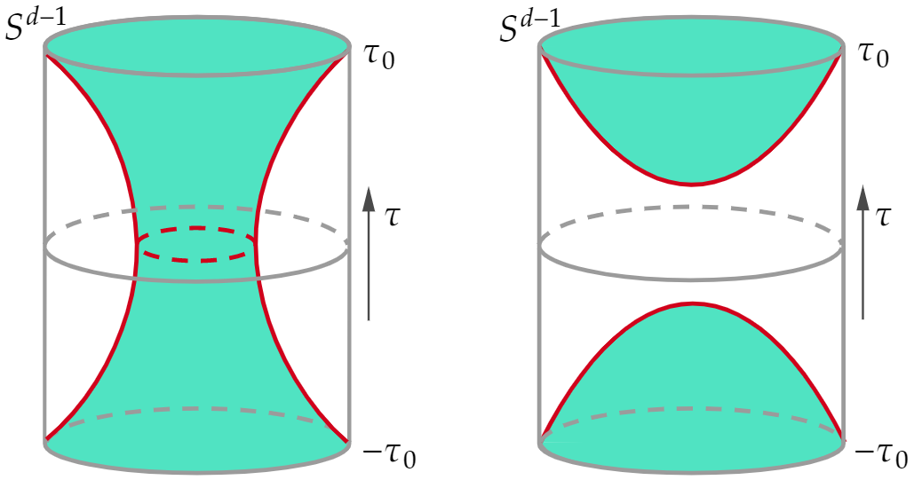
Figure 1: Left: connected EOW brane in Euclidean AdS_d+1-Schwarzschild geometry. Right: disconnected EOW brane in thermal-AdS_d+1.

The bulk Euclidean action is

$$I_{E}=-\frac{1}{16\pi G^{(d+1)}_{N}}\int_{N}d^{d+1}x\sqrt{g}(R-2\Lambda_{d+1})-\frac{1}{8\pi G^{(d+1)}_{N}}\int_{Q}d^{d}y\sqrt{h}(K-(d-1)T)\ ,$$ (1)

where $N$ represents the bulk and $Q$ represents the EOW brane, we omit the Gibbons-Hawking term on asymptotic boundary. $T$ is the constant tension of the EOW brane and we will see that it is related to the conformal boundary condition. The key assumption for the AdS_d+1/BCFT_d is that the induced metric $h_{ab}$ on the EOW brane preserves the boundary symmetry $SO(d,1)$ and satisfies Neumann boundary condition. The variation of the action to $h_{ab}$ leads to the Neumann boundary condition

$$K_{ab}-Kh_{ab}=(1-d)Th_{ab}\ .$$ (2)

Since the holographic BCFT_d defined on $S^{d-1}$ preserves spherical symmetry, the bulk dual will also preserve this symmetry. As a result, it must locally be described by Euclidean AdS_d+1-Schwarzschild geometry

$$ds^{2}=f(r)d\tau^{2}+\frac{dr^{2}}{f(r)}+r^{2}d\Omega_{d-1}^{2}\ ,$$ (3)

where

$$f(r)=\frac{r^{2}}{\ell^{2}}+1-\frac{r_{h}^{d-2}}{r^{d-2}}(\frac{r_{h}^{2}}{\ell^{2}}+1)\ .$$ (4)

$r_{h}$ is the horizon radius and $\ell$ is the AdS radius. Notice that the Euclidean time circle of black hole is compact and $[-\tau_{0},\tau_{0}]$ should be considered as part of the $\tau$-circle. The brane attached at $\tau=\pm\tau_{0}$ will also preserve the spherical symmetry and we can parameterize it as $r(\tau)$. Using the Neumann boundary condition eq. (2), we can find the brane trajectory satisfies

$$\frac{dr}{d\tau}=\pm\frac{f(r)}{Tr}\sqrt{f(r)-T^{2}r^{2}}\ .$$ (5)

The bulk metric eq.(3) generally have two different phases. It is known that $r_{h}=0$ corresponds to thermal-AdS_d+1 and $r_{h}>0$ corresponds to AdS_d+1-Schwarzschild. The transition between the two phases is known as Hawking-Page transition Hawking:1982dh ; Witten:1998zw . The Hawking-Page transition will also affect the EOW brane Fujita:2011fp ; Cooper:2018cmb ; Sully:2020pza ; Miyaji:2021ktr . In the thermal AdS_d+1 bulk, we will have two disconnected EOW branes. While in the AdS_d+1-Schwarzschild bulk, the EOW brane will be connected. This is a high temperature phase which dominates for a short time interval $[-\tau_{0},\tau_{0}]$. We will be mostly interested in this phase, shown in left of Fig. 1.

Since the Euclidean brane solution of eq. (5) is symmetric about the $\tau=0$ slice, we can take the $\tau=0$ bulk slice as initial time slice for a Lorentzian evolution. This is equivalent to apply an analytical continuation $t=-i\tau$ in the time direction. The Lorentzian bulk geometry is thermal-AdS_d+1 spacetime or AdS_d+1-Schwarzschild black hole. The brane trajectory satisfies

$$\frac{dr}{dt}=\pm\frac{f(r)}{Tr}\sqrt{T^{2}r^{2}-f(r)}\ .$$ (6)

The brane world-volume metric is given by

$$ds^{2} =-f(r)dt^{2}+\frac{f(r)(T^{2}r^{2}-f(r))}{T^{2}r^{2}}dt^{2}+r^{2}d\Omega_{d-1}^{2}$$ (7)

$$=-\frac{f(r)^{2}}{T^{2}r^{2}}dt^{2}+r^{2}d\Omega_{d-1}^{2}$$

$$=-dt_{p}^{2}+r^{2}(t_{p})d\Omega_{d-1}^{2}\ ,$$

where in the last step we define a new time $t_{p}$ satisfying $dt_{p}=\frac{f(r(t))}{Tr(t)}dt$ and $r(t_{p})$ is the scale factor. Below we can find that in the AdS_d+1-Schwarzschild black hole case, the scale factor corresponds to a big-bang big-crunch cosmology. For general dimensions, the brane trajectory need to be solved numerically. Now we focus on $d=2$ case where everything can be solved analytically. The $d=4$ case will be discussed in next section.

For $d=2$, the boundary state $|B\rangle_{\pm}$ is known as Cardy state Cardy:1989ir . The bulk is an Euclidean BTZ black hole Banados:1992wn ,

$$ds_{\mathrm{EBTZ}}^{2}=\frac{r^{2}-r_{h}^{2}}{\ell^{2}}d\tau^{2}+\frac{\ell^{2}}{r^{2}-r_{h}^{2}}dr^{2}+r^{2}d\theta^{2}\ .$$ (8)

The periodicity of the $\tau$ direction determines the temperature of the black hole, which is

$$\beta=\frac{2\pi\ell^{2}}{r_{h}}\ .$$ (9)

The brane trajectory $r(\tau)$ satisfies eq. (5),

$$\frac{dr}{d\tau}=\pm\frac{r^{2}-r_{h}^{2}}{T\ell^{2}r}\sqrt{\frac{r^{2}-r_{h}^{2}}{\ell^{2}}-T^{2}r^{2}}\ .$$ (10)

After integration we obtain the brane trajectory as

$$r(\tau) =\frac{r_{h}}{\sqrt{1-T^{2}\ell^{2}}}\sqrt{1+T^{2}\ell^{2}\tan^{2}\frac{r_{h}\tau}{\ell^{2}}}$$ (11)

$$=\frac{r_{h}}{\sqrt{1-T^{2}\ell^{2}}}\frac{1}{\cos\frac{r_{h}\tau^{\prime}}{\ell^{2}}}\ ,$$

where we have replaced $\tau$ with $\tau^{\prime}$ by

$$\tan\frac{r_{h}\tau^{\prime}}{\ell^{2}}=T\ell\tan\frac{r_{h}\tau}{\ell^{2}}\ .$$ (12)

We will see that $\tau^{\prime}$ is the brane conformal time. Notice that $\tau^{\prime}$ also belongs to $[-\tau_{0},\tau_{0}]$.

It is easy to see that the brane trajectory is symmetric about $\tau=0$, where $r(\tau)$ takes its minimal value, which equals to

$$r_{0}=\frac{r_{h}}{\sqrt{1-T^{2}\ell^{2}}}\ .$$ (13)

The Euclidean time $\tau_{0}$ can be obtained by subtracting half of the brane time from half of the whole time. It is related to the black hole temperature as

$$\tau_{0} =\frac{\beta}{2}-\int_{r_{0}}^{\infty}\frac{T\ell^{2}rdr}{(r^{2}-r_{h}^{2})\sqrt{\frac{r^{2}-r_{h}^{2}}{\ell^{2}}-T^{2}r^{2}}}$$ (14)

$$=\frac{\beta}{2}-\left(\frac{\pi\ell^{2}}{2r_{h}}-\frac{\ell^{2}\arctan\frac{\sqrt{r_{0}^{2}-r{{}_{H}}^{2}-T^{2}\ell^{2}r_{0}^{2}}}{T\ell r_{h}}}{r_{h}}\right)$$

$$=\frac{\beta}{2}-\frac{\pi\ell^{2}}{2r_{h}}$$

$$=\frac{\pi\ell^{2}}{2r_{h}}$$

$$=\frac{\beta}{4}\ .$$

It means that the brane trajectory always meets the boundary at antipodal points in the $(r,\tau)$ disc. The brane trajectory is shown in Fig. 2.

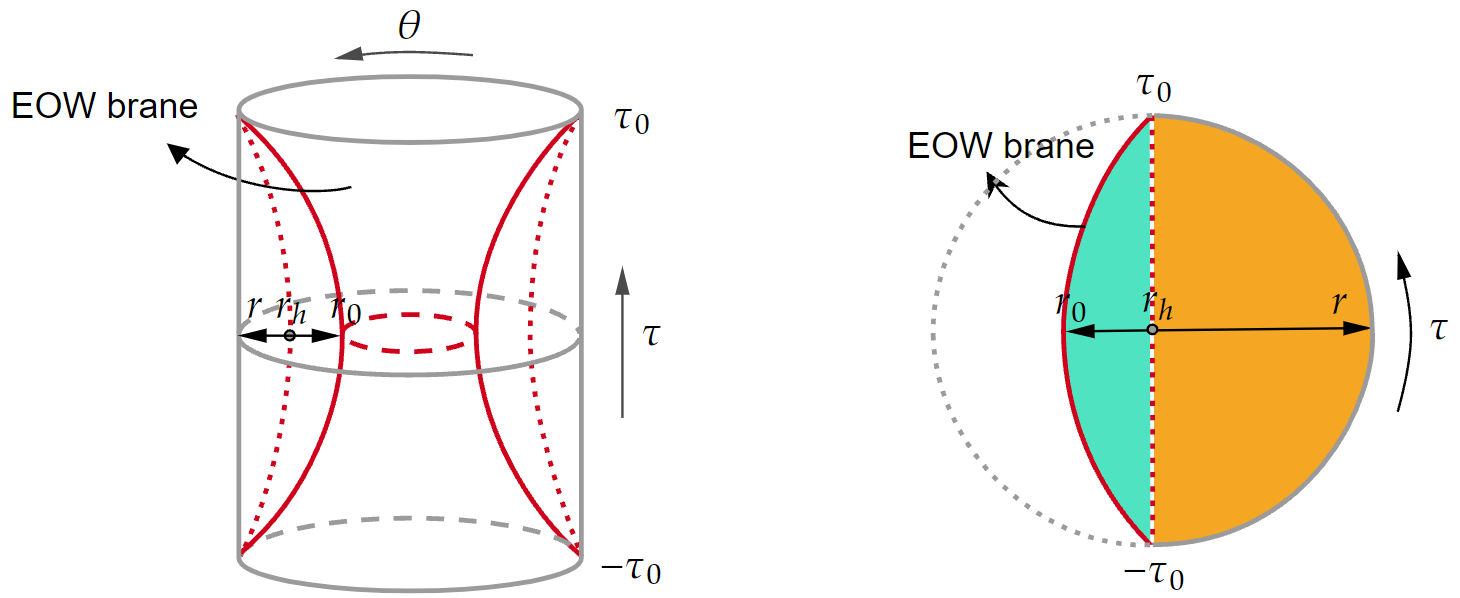
Figure 2: Left: Euclidean geometry for the brane trajectory. The red dotted line is the zero tension brane. The red solid line represents any $T>0$ brane. Right: $(\tau,r)$ disc expression, where each point has a $S^{1}$ of radius $r$.

Substituting the brane trajectory eq. (11) into the bulk metric eq. (8), we obtain the induced metric on the brane as

$$ds_{brane}^{2} =\frac{(r^{2}-r_{h}^{2})^{2}}{T^{2}\ell^{4}r^{2}}d\tau^{2}+r^{2}d\theta^{2}$$ (15)

$$=\frac{r_{h}^{2}}{1-T^{2}\ell^{2}}\frac{T^{2}(1+\tan^{2}\frac{r_{h}\tau}{\ell^{2}})^{2}}{1+T^{2}\ell^{2}\tan^{2}\frac{r_{h}\tau}{\ell^{2}}}d\tau^{2}+\frac{r_{h}^{2}}{1-T^{2}\ell^{2}}(1+T^{2}\ell^{2}\tan^{2}\frac{r_{h}\tau}{\ell^{2}})d\theta^{2}$$

$$=\frac{r_{h}^{2}}{1-T^{2}\ell^{2}}\frac{(1+\tan^{2}\frac{r_{h}\tau}{\ell^{2}})^{2}}{1+T^{2}\ell^{2}\tan^{2}\frac{r_{h}\tau}{\ell^{2}}}\frac{\cos^{4}\frac{r_{h}\tau}{\ell^{2}}}{\cos^{4}\frac{r_{h}\tau^{\prime}}{\ell^{2}}}\frac{1}{\ell^{2}}d\tau^{\prime 2}+\frac{r_{h}^{2}}{1-T^{2}\ell^{2}}(1+T^{2}\ell^{2}\tan^{2}\frac{r_{h}\tau}{\ell^{2}})d\theta^{2}$$

$$=\frac{r_{0}^{2}}{\cos^{2}\frac{r_{h}\tau^{\prime}}{\ell^{2}}}(\frac{1}{\ell^{2}}d\tau^{\prime 2}+d\theta^{2})\ .$$

In the third line, we have used $\tan\frac{r_{h}\tau^{\prime}}{\ell^{2}}=T\ell\tan\frac{r_{h}\tau}{\ell^{2}}$. And from the last line, we can easily check that it is a hyperbolic space with scalar curvature $R_{brane}=-\frac{2(1-T^{2}\ell^{2})}{\ell^{2}}$. This metric is conformally equivalent to a finite cylinder metric $ds_{brane}^{2}=\Omega^{-2}(\tau^{\prime})ds_{cyl}^{2}=\Omega^{-2}(\tau^{\prime})(\frac{1}{\ell^{2}}d\tau^{\prime 2}+d\theta^{2})$ with a conformal factor $\Omega(\tau^{\prime})=\frac{1}{r_{0}}\cos\frac{r_{h}\tau^{\prime}}{\ell^{2}}$.

Let us apply an analytical continuation $t=-i\tau$ and the brane trajectory is

$$r(t) =\frac{r_{h}}{\sqrt{1-T^{2}\ell^{2}}}\sqrt{1-T^{2}\ell^{2}\tanh^{2}\frac{r_{h}t}{\ell^{2}}}$$ (16)

$$=\frac{r_{h}}{\sqrt{1-T^{2}\ell^{2}}}\frac{1}{\cosh\frac{r_{h}t^{\prime}}{\ell^{2}}}\ ,$$

where $t^{\prime}$ is defined as $\tanh\frac{r_{h}t^{\prime}}{\ell^{2}}=T\ell\tanh\frac{r_{h}t}{\ell^{2}}$. Using

$$\frac{dr}{dt_{p}}=\frac{dr}{dt}\cdot\frac{dt}{dt_{p}}=\pm\sqrt{T^{2}r^{2}-\frac{r^{2}-r_{h}^{2}}{\ell^{2}}}\ ,$$ (17)

the scale factor is obtained as $r(t_{p})=r_{0}\cos\frac{r_{h}t_{p}}{\ell r_{0}}$, which describes to a big-bang big-crunch cosmology.

2.2 Bulk defect extremal surface

Quantum extremal surface was proposed to compute the holographic entanglement entropy including the contribution of bulk quantum matter Faulkner:2013ana ; Lewkowycz:2013nqa ; Engelhardt:2014gca

$$S_{A}=\min\left\{{\mathrm{ext}\,{S_{gen}}}\right\}=\min\left\{\mathrm{ext_{\Gamma}}\left[\frac{\operatorname{Area}(\Gamma)}{4G_{N}}+S_{\text{bulk}}\right]\right\}\ ,$$ (18)

where $\Gamma$ is a co-dimension two surface in AdS bulk which is homologous with subregion $A$.

Quantum extremal surface has been generalized to holographic dualities with defects Deng:2020ent . In quantum field theory with defects, entanglement entropy is generally corrected by the defect. The same thing happens in the bulk. For instance, in Takayanagi:2011zk it was proposed that the entanglement entropy of an interval $[0,x_{0}]$ on the BCFT can be calculated holographically by the bulk RT surface Ryu:2006bv , as illustrated in Fig. 3. Now if we take the brane as a defect in the bulk and add conformal matter on it, it is obvious that one should include the contribution from these matter when calculating the entanglement entropy. Thus the RT formula should be modified to the defect extremal surface (DES) formula, which is given by Deng:2020ent

$$S_{A}^{\mathrm{DES}}=\min_{\Gamma,X}\left\{\operatorname{ext}_{\Gamma,X}\left[\frac{\operatorname{Area}(\Gamma)}{4G_{N}}+S_{\text{defect }}[D]\right]\right\},\quad X=\Gamma\cap D\ ,$$ (19)

where $\Gamma$ is a co-dimension two surface in AdS bulk and $X$ is the lower dimensional entangling surface determined by the intersection of $\Gamma$ and the defect $D$.

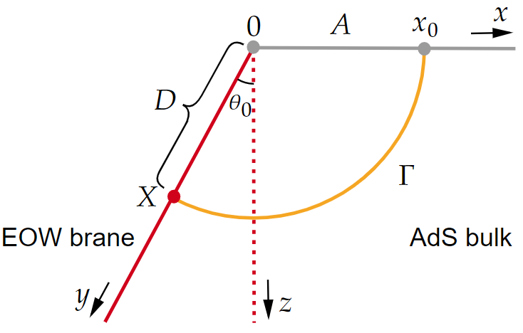
Figure 3: The RT surface $\Gamma$ for an interval $A:=[0,x_{0}]$ that contains the boundary. When the boundary of the BCFT is contained in the interval, $\Gamma$ will extend to the EOW brane, on which conformal matter is distributed.

In this note, we will apply the defect extremal surface formula to two-dimensional cosmology at the end of the world brane.

Let us consider the entanglement entropy of a large interval $A$ on the BCFT₂. The end points of the interval $A$ are $w_{1}=(-\theta_{1},\frac{\tau_{1}}{\ell})$ and $w_{2}=(\theta_{1},\frac{\tau_{1}}{\ell})$ at fixed time $\tau=\tau_{1}$ slice. The DES calculation in this time slice is depicted in Fig. 4. Using the defect extremal surface formula, the bulk generalized entropy is

$$S_{gen}=\frac{\text{Area}}{4G_{N}^{(3)}}+S_{A^{\prime}}\ ,$$ (20)

where $S_{A^{\prime}}$ is the entanglement entropy of the interval in brane conformal field theory.

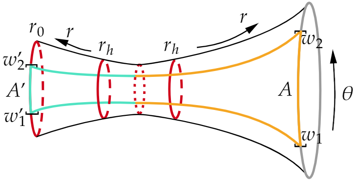
Figure 4: An illustration of bulk DES calculation in $t=t_{1}$ slice.

In the following, $S_{A^{\prime}}$ is found to be a constant. Let us use replica trick Calabrese:2004eu to compute $S_{A^{\prime}}$. The brane metric is

$$ds_{brane}^{2}=\frac{r_{0}^{2}}{\cos^{2}\frac{r_{h}\tau^{\prime}}{\ell^{2}}}(\frac{1}{\ell^{2}}d\tau^{\prime 2}+d\theta^{2})\ .$$ (21)

It’s conformally equivalent to a cylinder

$$ds_{cylinder}^{2}=\frac{1}{\ell^{2}}d\tau^{\prime 2}+d\theta^{2}\ ,$$ (22)

with conformal factor $\Omega(\tau^{\prime})=\frac{1}{r_{0}}\cos\frac{r_{h}\tau^{\prime}}{\ell^{2}}$. The cylinder can be described by complex coordinate $w^{\prime}=\theta+i\frac{\tau^{\prime}}{\ell}$. We then map the cylinder onto an upper half-plane (UHP) by

$$w^{\prime}=-i\frac{\tau_{0}}{\ell}+\frac{\ell}{r_{h}}\log z$$ (23)

and the metric becomes

$$ds^{2}=\frac{1}{\ell^{2}}d\tau^{\prime 2}+d\theta^{2}=\frac{\ell^{2}}{r_{h}^{2}z^{2}}dzd\bar{z}\ ,$$ (24)

where $z=x+iy$ is the coordinates of the complex plane. The conformal factor is $\Omega^{\prime}(z)=|\frac{r_{h}z}{\ell}|$. Eventually we map the brane to the UHP and the two boundaries of Euclidean brane now becomes a single boundary. The end points of the interval are mapped to

$$z_{1}=e^{-\frac{r_{h}}{\ell}\theta_{1}+i(\frac{r_{h}\tau^{\prime}_{1}}{\ell^{2}}+\frac{\pi}{2})}\ ,\;\;\;z_{2}=e^{\frac{r_{h}}{\ell}\theta_{1}+i(\frac{r_{h}\tau^{\prime}_{1}}{\ell^{2}}+\frac{\pi}{2})}\ .$$ (25)

The whole process of the conformal map is illustrated in Fig. 5.

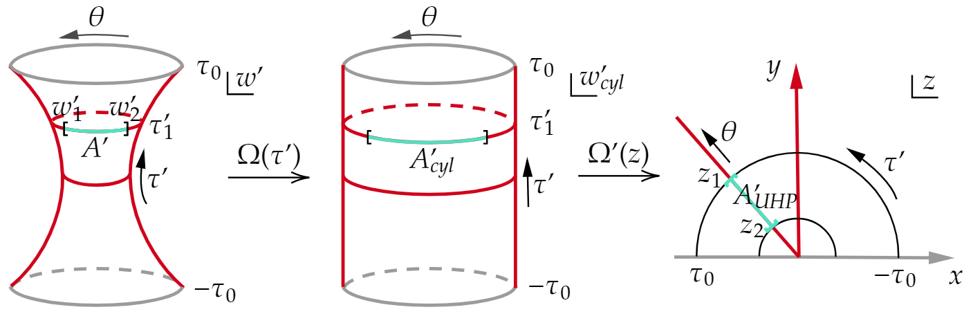
Figure 5: Conformal mapping from brane to the UHP. The green line represents the interval.

The Renyi entropy for an interval $A^{\prime}_{\mathrm{UHP}}$ is related to the two point function of twist operators in UHP by

$$S_{A^{\prime}_{\mathrm{UHP}}}^{n}=\frac{1}{1-n}\log\mathrm{Tr}(\rho_{A^{\prime}_{\mathrm{UHP}}}^{n})=\frac{1}{1-n}\log\langle\phi_{n}(z_{1},\overline{z}_{1})\overline{\phi}_{n}(z_{2},\overline{z}_{2})\rangle_{b}.$$ (26)

where $b$ represent the conformal boundary condition of the UHP CFT. The doubling trick Recknagel:2013uja indicates that the two point functions in the UHP have the same functional form as the chiral four point functions in the whole plane,

$$\langle\phi_{n}(z_{1},\overline{z}_{1})\overline{\phi}_{n}(z_{2},\overline{z}_{2})\rangle_{b}\simeq\langle\phi_{n}(z_{1})\overline{\phi}_{n}(z_{2})\phi_{n}(\overline{z}_{1})\overline{\phi}_{n}(\overline{z}_{2})\rangle.$$ (27)

We can expand the two point function in a bulk channel or a boundary channel McAvity:1995zd . The bulk channel is given by bulk operator expansion (OPE) and the boundary channel is given by boundary operator expansion (BOE). Using doubling trick, the expansion can be expressed as a sum over the conformal blocks of chiral four point function, we refer to Ref. Sully:2020pza for more details. We sketch these two channels in Fig. 6. Assuming the vacuum block dominance Hartman:2013mia ; Faulkner:2013yia ; Sully:2020pza , the two point function in two different channels in the large central charge limit is given by

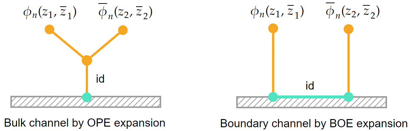
Figure 6: The UHP two point function through different channels.

$$\begin{split}\begin{cases}\langle\phi_{n}(z_{1},\overline{z}_{1})\overline{\phi}_{n}(z_{2},\overline{z}_{2})\rangle_{b}=\frac{g_{b}^{2(1-n)}|z_{1}-z_{2}|^{-2d_{n}}}{\epsilon^{\prime-2d_{n}}},\;\;\;\mathrm{OPE\,\,channel},\\ \langle\phi_{n}(z_{1},\overline{z}_{1})\overline{\phi}_{n}(z_{2},\overline{z}_{2})\rangle_{b}=\frac{g_{b}^{2(1-n)}(4y_{1}y_{2})^{-d_{n}}}{\epsilon^{\prime-2d_{n}}},\;\;\;\mathrm{~{}BOE\,\,channel},\end{cases}\end{split}$$ (28)

where $d_{n}=\frac{c^{\prime}}{12}(n-\frac{1}{n})$ is the conformal dimension of the twist operator, $\epsilon^{\prime}$ is the UV-cutoff and $g_{b}$ is related to the boundary entropy. Combining the conformal factor $(\Omega^{\prime}(z)\cdot\Omega(\tau^{\prime}))^{d_{n}}=|\frac{r_{h}z}{\ell}\cdot\frac{1}{r_{0}}\cos\frac{r_{h}\tau^{\prime}}{\ell^{2}}|^{d_{n}}$, the Renyi entropy of the CFT_brane is

$$S_{A^{\prime}}^{n} =\frac{1}{1-n}\log\mathrm{Tr}(\rho_{A^{\prime}}^{n})$$ (29)

$$=\frac{1}{1-n}\log\bigg{[}(\Omega^{\prime}(z_{1})\cdot\Omega(\tau^{\prime}_{1}))^{d_{n}}(\Omega^{\prime}(z_{2})\cdot\Omega(\tau^{\prime}_{1}))^{d_{n}}\langle\phi_{n}(z_{1},\overline{z}_{1})\overline{\phi}_{n}(z_{2},\overline{z}_{2})\rangle_{b}\bigg{]}\ .$$

The Renyi entropy of $A^{\prime}$ is obtained by substitute its coordinate eq. (25) into eq. (29). For the OPE channel, the Renyi entropy is

$$S_{A^{\prime}}^{n} =\frac{1}{1-n}\log\bigg{[}(|\frac{r_{0}^{2}}{\cos^{2}\frac{r_{h}\tau^{\prime}_{1}}{\ell^{2}}}\cdot\frac{\ell^{2}}{r_{h}^{2}z_{1}z_{2}}|\cdot\frac{|z_{1}-z_{2}|^{2}}{\epsilon^{\prime 2}})^{-d_{n}}g_{b}^{2(1-n)}\bigg{]}$$ (30)

$$=\frac{c^{\prime}}{12}\frac{n+1}{n}\log(\frac{r_{0}^{2}}{\cos^{2}\frac{r_{h}\tau^{\prime}_{1}}{\ell^{2}}}\cdot\frac{\ell^{2}}{r_{h}^{2}}\cdot\frac{4\sinh^{2}\frac{r_{h}\theta_{1}}{\ell}}{\epsilon^{\prime 2}})+2\log g_{b}$$

$$=\frac{c^{\prime}}{6}\frac{n+1}{n}\log\frac{2r_{0}\ell\sinh\frac{r_{h}\theta_{1}}{\ell}}{r_{h}\epsilon^{\prime}\cos\frac{r_{h}\tau^{\prime}_{1}}{\ell^{2}}}+2\log g_{b}\ .$$

For the BOE channel, the Renyi entropy is

$$S_{A^{\prime}}^{n} =\frac{1}{1-n}\log\bigg{[}(|\frac{r_{0}^{2}}{\cos^{2}\frac{r_{h}\tau^{\prime}_{1}}{\ell^{2}}}\cdot\frac{\ell^{2}}{r_{h}^{2}z_{1}z_{2}}|\cdot\frac{4y_{1}y_{2}}{\epsilon^{\prime 2}})^{-d_{n}}g_{b}^{2(1-n)}\bigg{]}$$ (31)

$$=\frac{c^{\prime}}{12}\frac{n+1}{n}\log(\frac{r_{0}^{2}}{\cos^{2}\frac{r_{h}\tau^{\prime}_{1}}{\ell^{2}}}\cdot\frac{\ell^{2}}{r_{h}^{2}}\cdot\frac{4\cos^{2}\frac{r_{h}\tau^{\prime}_{1}}{\ell^{2}}}{\epsilon^{\prime 2}})+2\log g_{b}$$

$$=\frac{c^{\prime}}{6}\frac{n+1}{n}\log\frac{2r_{0}\ell}{r_{h}\epsilon^{\prime}}+2\log g_{b}\ .$$

After taking the limit $n\rightarrow 1$, $S_{A^{\prime}}$ becomes

$$S_{A^{\prime}}=\lim_{n\rightarrow 1}S_{A^{\prime}}^{n}=\begin{cases}\frac{c^{\prime}}{3}\log\frac{2r_{0}\ell\sinh\frac{r_{h}\theta_{1}}{\ell}}{r_{h}\cos\frac{r_{h}\tau^{\prime}_{1}}{\ell^{2}}\epsilon^{\prime}}+2\log g_{b}\ \ \ ,\ \ \ \mathrm{OPE\ \ channel}\ ,\\ \frac{c^{\prime}}{3}\log\frac{2r_{0}\ell}{r_{h}\epsilon^{\prime}}+2\log g_{b}\ \ \ \ \ \ \ \ \ \ \ \ \ ,\ \ \ \mathrm{BOE\ \ channel}\ .\end{cases}$$ (32)

For a large enough interval $A$, the entanglement wedge will include the brane region and the BOE channel will be of our interest. In this case, the entropy of the interval is

$$S_{A^{\prime}}=\frac{c^{\prime}}{3}\log\frac{2r_{0}\ell}{r_{h}\epsilon^{\prime}}+2\log g_{b}\ ,$$ (33)

which is a constant.

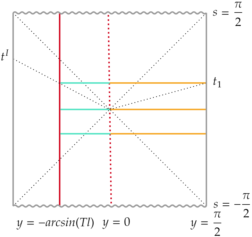
Figure 7: BTZ black hole in $s$-$y$ coordinate. The red solid line is the brane with tension $T$, the red dashed line is the brane with tension zero. The line orthogonal to the brane is the RT surface.

Below we will assume that the central charge $c^{\prime}$ of the brane CFT is the same as the central charge $c$ of holographic BCFT₂ and we take the boundary entropy $\log g_{b}$ of the brane CFT to be zero, then

$$S_{A^{\prime}}=\frac{c}{3}\log\frac{2r_{0}\ell}{r_{h}\epsilon^{\prime}}\ .$$ (34)

To compute $S_{A}^{\mathrm{RT}}$, let us work in Lorentzian signature and change from Schwarzschild $t$-$r$ coordinate to Kruskal-type $s$-$y$ coordinate by replacing

$$t=\frac{\ell^{2}}{2r_{h}}\ln\left(-\frac{\tan\left(\frac{s+y}{2}\right)}{\tan\left(\frac{s-y}{2}\right)}\right),\ \ \ r=r_{h}\frac{1-\tan\left(\frac{s+y}{2}\right)\tan\left(\frac{s-y}{2}\right)}{1+\tan\left(\frac{s+y}{2}\right)\tan\left(\frac{s-y}{2}\right)}\ .$$ (35)

In $s$-$y$ coordinate, the maximally extended BTZ black hole takes the form

$$ds_{\mathrm{BTZ}}^{2}=\frac{1}{\cos^{2}y}(-\ell^{2}ds^{2}+\ell^{2}dy^{2}+r_{h}^{2}\cos^{2}(s)d\theta^{2})\ .$$ (36)

After this transformation, the brane trajectory in $s$-$y$ coordinate is

$$y=-\arcsin(T\ell)\ ,$$ (37)

which says that the brane stays in constant $y$ slice shown in red line in Fig. 7.

The RT surface and the brane are perpendicular to each other at the intersection point. The cutoff surface is $r_{max}=\frac{\ell^{2}}{\epsilon}$. We then obtain $S_{A}^{\mathrm{RT}}$ as

$$\begin{split}S_{A}^{\mathrm{RT}}=\begin{cases}\frac{c}{3}\log\frac{2\ell^{2}\sinh\frac{r_{h}\theta_{1}}{\ell}}{r_{h}\epsilon}\;\;\;,\;\;\;\mathrm{conn.}\\ \frac{c}{3}\log\frac{2\ell^{2}\cosh\frac{r_{h}t_{1}}{\ell^{2}}}{r_{h}\epsilon}+\frac{c}{3}\log\sqrt{\frac{1+T\ell}{1-T\ell}}\;\;\;,\;\;\;\mathrm{disc.}\end{cases}\end{split}$$ (38)

In our case, the disconnected phase dominates for a large interval.

Adding the two terms together, the holographic entanglement entropy calculated by DES formula is

$$S_{A}^{\mathrm{DES}}=S_{A}^{\mathrm{RT}}+S_{A^{\prime}}=\frac{c}{3}\log\frac{2r_{0}\ell}{r_{h}\epsilon^{\prime}}+\frac{c}{3}\log\frac{2\ell^{2}\cosh\frac{r_{h}t_{1}}{\ell^{2}}}{r_{h}\epsilon}+\frac{c}{3}\log\sqrt{\frac{1+T\ell}{1-T\ell}}\ .$$ (39)

2.3 Island formula for cosmology at the end of the world

Let us justify the entanglement entropy result obtained in the previous subsection by island formula Almheiri:2019hni . An effective $2d$ description for the bulk with a brane can be obtained by combining partial Randall-Sundrum reduction and AdS/CFT correspondence. The procedure of partial reduction is as follows. The bulk is decomposed into two parts by the zero tension brane, whose trajectory is

$$r(\tau^{\prime})=\frac{r_{h}}{\cos\frac{r_{h}\tau^{\prime}}{\ell^{2}}}\ ,$$ (40)

which intersects with the bifurcation point at $\tau^{\prime}=0$. Since no physical degrees of freedom is living on the brane, it can be viewed as a transparent boundary condition.

We divide the bulk region bounded by the finite tension brane into two parts: reduction region and duality region as shown in Fig. 8. The whole process of partial reduction is as follows. For the reduction region, we employ Randall-Sundrum reduction Randall:1999ee ; Randall:1999vf and obtain a gravity theory on the brane, coupled with CFT matter. For the duality region, we use the ordinary AdS/CFT and obtain a boundary conformal field theory with zero boundary entropy. The brane CFT and holographic BCFT₂ are glued together with transparent boundary condition, which is essentially the dual of the imaginary bulk zero tension brane.

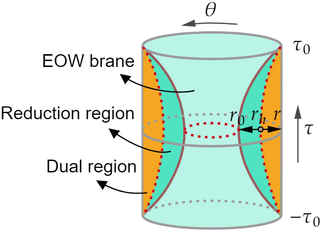
Figure 8: The bulk region is divided into two parts by the zero tension brane. A $2d$ effective theory is obtained by applying partial Randall-Sundrum and AdS/CFT to reduction region and dual region respectively.

By integrating the warp factor from the zero tension brane to the $T$ tension brane Akal:2020wfl , the Newton constant on the brane is

$$\frac{1}{4G_{brane}} =\frac{\ell}{4G_{N}^{(3)}}\int_{-\arcsin(T\ell)}^{-\arcsin 0}\frac{dy}{\cos y}$$ (41)

$$=\frac{\ell}{4G_{N}^{(3)}}\left[-\log(\cos\frac{y}{2}-\sin\frac{y}{2})+\log(\cos\frac{y}{2}+\sin\frac{y}{2})\right]\Big{|}_{-\arcsin(T\ell)}^{-\arcsin 0}$$

$$=\frac{\ell}{4G_{N}^{(3)}}\log\sqrt{\frac{1+T\ell}{1-T\ell}}\ .$$

Now we can use the island formula to compute the entanglement entropy for the same boundary interval $A$. The generalized entropy is expressed as

$$S_{gen}=\frac{\text{Area}(\partial I)}{4G_{brane}}+S(A\cup I)\ ,$$ (42)

where $I$ represents the island region. We can also view the $2d$ brane after partial reduction as a bra-ket wormhole Chen:2020tes . Notice that in Euclidean signature, the brane time $\tau^{\prime}$ can be treated as a natural extension of the boundary time $\tau$, as shown in Fig. 9. Therefore the island lies between $w_{1}^{I}=(-\theta_{1},\frac{\tau_{0}+\tau_{1}^{I}}{\ell})$ and $w_{2}^{I}=(\theta_{1},\frac{\tau_{0}+\tau_{1}^{I}}{\ell})$. Since the boundary of the island has two points, the area term is

$$S^{\prime} =\frac{\text{Area}(\partial I)}{4G_{brane}}$$ (43)

$$=2\cdot\frac{1}{4G_{brane}}$$

$$=\frac{\ell}{2G_{N}^{(3)}}\log\sqrt{\frac{1+T\ell}{1-T\ell}}$$

$$=\frac{c}{3}\log\sqrt{\frac{1+T\ell}{1-T\ell}}\ ,$$

where we have substituted $G_{N}^{(3)}=\frac{3\ell}{2c}$ and taken the area of a point as $1$. It is easy to see that $S^{\prime}$ is a constant, which means that we only need to extremize $S(A\cup I)$ to determine the location of the island.

In the large interval limit, the entropy $S(A\cup I)$ can be decomposed as

$$S(A\cup I)=S[w_{1},w_{1}^{I}]+S[w_{2},w_{2}^{I}]\ .$$ (44)

Similar to the previous section, it can be calculated by twist operator correlation function. Using the conformal transformation in eq. (21)(23), we can map CFT_brane to UHP and $w_{1}^{I}$, $w_{2}^{I}$ to

$$z_{1}^{I}=e^{-\frac{r_{h}\theta_{1}}{\ell}+i\frac{r_{h}\tau_{1}^{I}}{\ell^{2}}}\ ,\;\;\;z_{2}^{I}=e^{\frac{r_{h}\theta_{1}}{\ell}+i\frac{r_{h}\tau_{1}^{I}}{\ell^{2}}}\ .$$ (45)

The conformal factor is $\Omega^{\prime}(z)\cdot\Omega(\tau^{\prime})=|\frac{r_{h}z}{\ell}\cdot\frac{1}{r_{0}}\cos\frac{r_{h}\tau^{\prime}}{\ell^{2}}|$. Simultaneously, using the conformal transformation

$$w=i\frac{\tau_{0}}{\ell}+\frac{\ell}{r_{h}}\log z\ ,$$ (46)

we map the holographic BCFT₂ to the down half-plane (DHP) with conformal factor $\Omega\cdot\Omega^{\prime}(z)=\frac{1}{\ell}\cdot|\frac{r_{h}z}{\ell}|$. $w_{1}$ and $w_{2}$ are mapped to $z_{1}=e^{-\frac{r_{h}\theta_{1}}{\ell}+i(\frac{r_{h}\tau_{1}}{\ell^{2}}-\frac{\pi}{2})}$ and $z_{2}=e^{\frac{r_{h}\theta_{1}}{\ell}+i(\frac{r_{h}\tau_{1}}{\ell^{2}}-\frac{\pi}{2})}$ as shown in Fig. 9.

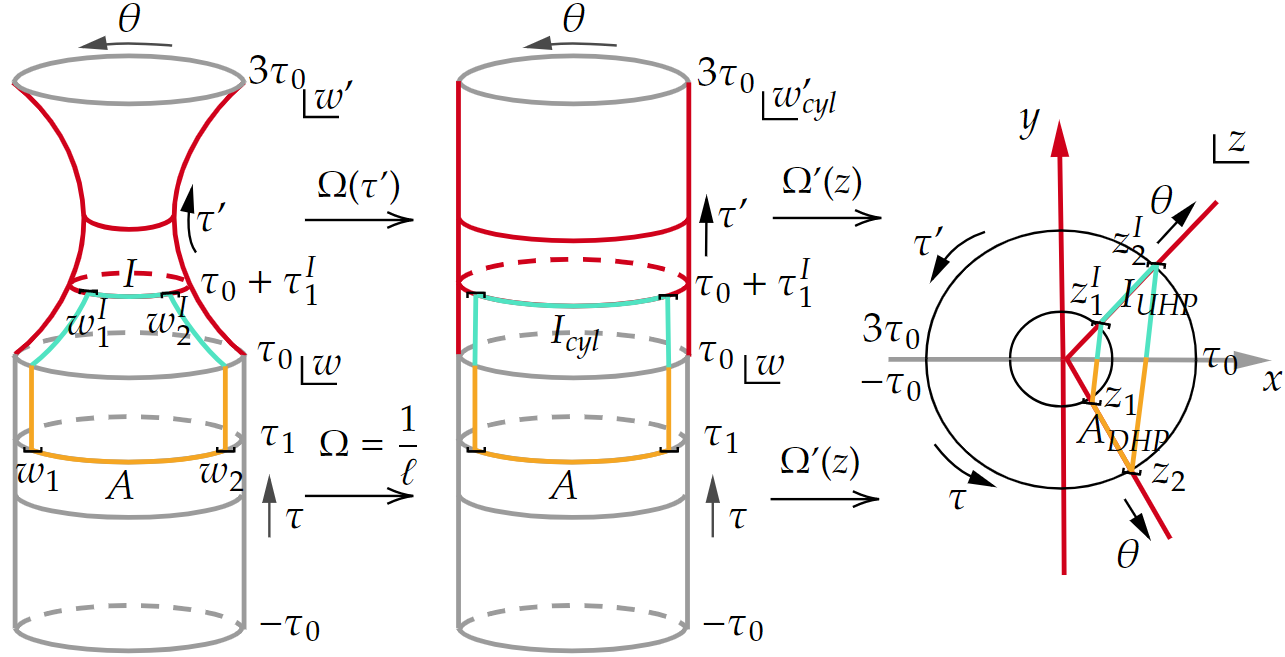
Figure 9: Conformal maps from the brane and bulk to a whole complex plane for island calculation.

The entropy between $z_{1}$ and $z_{1}^{I}$ is

$$S[z_{1},z_{1}^{I}]=\frac{c}{6}\log\frac{|z_{1}^{I}-z_{1}|^{2}}{\epsilon^{\prime}\epsilon}\ .$$ (47)

Combining with the conformal factor, the entropy in the original coordinate is

$$S[w_{1},w^{I}_{1}] =\frac{c}{6}\log\frac{|z_{1}^{I}-z_{1}|^{2}}{\Omega^{\prime}(z_{1}^{I})\Omega(\tau_{1}^{I})\epsilon^{\prime}\cdot\Omega^{\prime}(z_{1})\epsilon}$$ (48)

$$=\frac{c}{6}\log\frac{|z_{1}^{I}-z_{1}|^{2}}{|\frac{r_{h}z_{1}^{I}}{\ell}\cdot\frac{1}{r_{0}}\cos(\frac{r_{h}\tau_{1}^{I}}{\ell^{2}}+\frac{\pi}{2})|\epsilon^{\prime}\cdot|\frac{r_{h}z_{1}}{\ell^{2}}|\epsilon}$$

$$=\frac{c}{6}\log\frac{r_{0}\ell^{3}|e^{i\frac{r_{h}\tau_{1}^{I}}{\ell^{2}}}-e^{i(\frac{r_{h}\tau_{1}}{\ell^{2}}-\frac{\pi}{2})}|^{2}}{\epsilon^{\prime}\epsilon r_{h}^{2}\sin\frac{r_{h}\tau_{1}^{I}}{\ell^{2}}}$$

$$=\frac{c}{6}\log\frac{2r_{0}\ell^{3}(1+\sin\frac{r_{h}(\tau_{1}^{I}-\tau_{1})}{\ell^{2}})}{\epsilon^{\prime}\epsilon r_{h}^{2}\sin\frac{r_{h}\tau_{1}^{I}}{\ell^{2}}}\ .$$

Since there is no $\theta$ dependence, $S[w_{1},w_{1}^{I}]$ and $S[w_{2},w_{2}^{I}]$ are the same. $S(A\cup I)$ is given by

$$S(A\cup I)=S[w_{1},w_{1}^{I}]+S[w_{2},w_{2}^{I}]=2S[w_{1},w_{1}^{I}]\ .$$ (49)

Extremizing it with respect to $\tau_{1}^{I}$, the location of the island satisfies

$$\partial_{\tau_{1}^{I}}S(A\cup I)=\frac{\cos\frac{r_{h}\tau_{1}^{I}}{\ell^{2}}-\sin\frac{r_{h}\tau_{1}}{\ell^{2}}}{(\sin\frac{r_{h}(\tau_{1}-\tau_{1}^{I})}{\ell^{2}}-1)\sin\frac{r_{h}\tau_{1}^{I}}{\ell^{2}}}=0\ .$$ (50)

The solution is

$$\frac{r_{h}\tau_{1}^{I}}{\ell^{2}}=\frac{\pi}{2}-\frac{r_{h}\tau_{1}}{\ell^{2}}\ .$$ (51)

Back to the brane time, one can check that the island appears in the future to boundary subregion in $\tau$ coordinate. This is in agreement with bulk RT surface shown in Fig. 7.

Substituting eq. (51) into eq. (49), $S(A\cup I)$ takes its extremal value

$$S_{min}(A\cup I)=\frac{c}{3}\log\frac{2r_{0}\ell}{r_{h}\epsilon^{\prime}}+\frac{c}{3}\log\frac{2\ell^{2}\cos\frac{r_{h}\tau_{1}}{\ell^{2}}}{r_{h}\epsilon}\ .$$ (52)

So the entanglement entropy for subregion $A$ calculated by island formula is

$$S_{A} =\mathrm{Min}_{I}\ S_{gen}$$ (53)

$$=\frac{\mathrm{Area}(\partial I)}{4G_{brane}}+S_{min}(A\cup I)$$

$$=\frac{c}{3}\log\frac{2r_{0}\ell}{r_{h}\epsilon^{\prime}}+\frac{c}{3}\log\frac{2\ell^{2}\cos\frac{r_{h}\tau_{1}}{\ell^{2}}}{r_{h}\epsilon}+\frac{c}{3}\log\sqrt{\frac{1+T\ell}{1-T\ell}}\ .$$

After the analytic continuation to real time

$$S_{A}=\frac{c}{3}\log\frac{2r_{0}\ell}{r_{h}\epsilon^{\prime}}+\frac{c}{3}\log\frac{2\ell^{2}\cosh\frac{r_{h}t_{1}}{\ell^{2}}}{r_{h}\epsilon}+\frac{c}{3}\log\sqrt{\frac{1+T\ell}{1-T\ell}}\ ,$$ (54)

it matches the DES result eq. (39) precisely.

3 Cosmology from partial reduction in $d=4$

In this section, we generalize the partial reduction to $4d$ cosmology. We will first study the partial reduction for Karch-Randall brane Karch:2000ct in pure AdS₅ space. Based on this, we then propose a proper partial reduction for a $4d$ cosmology at the end of the world brane. We also calculate the boundary entropy associated to the boundary state in the Euclidean cosmology model. Demanding the boundary entropy as an area entropy on the brane after partial reduction, we deduce the Newton constant.

3.1 Partial Randall-Sundrum reduction in AdS₅

In Randall-Sundrum II reduction Randall:1999vf , we consider a Minkowski brane in AdS₅ and the brane tension has to be fine tuned. In particular, there is a massless graviton localized on the brane. However, if we consider AdS₄ Karch-Randall brane embedded in AdS₅ Karch:2000ct , the massless mode is missing because it is non-normalizable. Apart from the brane, the asymptotical boundary of AdS₅ in this case also attracts massless graviton significantly. We propose partial reduction to avoid this problem. In partial reduction, we split the whole bulk into two parts: one is the region between Karch-Randall brane and zero tension brane and the other is the remaining part. The brane gravity only comes from the reduction of the first part and the dynamics of the remaining part can be translated into a boundary conformal field theory coupled to the brane gravity. Note that this does not mean that the full reduction is wrong, rather it means that we can decompose the whole bulk and leave some of the bulk dynamics to the asymptotical boundary. This decomposition procedure has been justified in great detail Deng:2020ent ; Chu:2021gdb ; Li:2021dmf in the recent understanding of black hole information problem. In particular, it reproduces results from island formula precisely. We will demonstrate here the existence of a normalizable zero mode as well as a well-defined Newton constant in partial reduction. We will also discuss the relation between boundary entropy and Newton constant.

3.1.1 Localized gravity by partial reduction

Let us consider the bulk of AdS_d+1/BCFT_d. The bulk action is

$$I=\frac{1}{16\pi G^{(d+1)}_{N}}\int_{N}d^{d+1}x\sqrt{-g}(R-2\Lambda_{d+1})+\frac{1}{8\pi G^{(d+1)}_{N}}\int_{Q}d^{d}y\sqrt{-h}(K-(d-1)T)\ ,$$ (55)

where $N$ represents the bulk and $Q$ represents the EOW brane. $T$ is the constant tension of the EOW brane. The variation of the action with respect to the brane metric $h_{ab}$ leads to the Neumann boundary condition

$$K_{ab}-Kh_{ab}=(1-d)Th_{ab}\ .$$ (56)

One can easily check that a AdS_d+1 spacetime with a AdS_d embedding brane is a solution. For $d=4$, the bulk metric is given by

$$ds^{2}=dr^{2}+\cosh^{2}\frac{r}{\ell}\cdot\frac{\ell^{2}}{z^{2}}(-dt^{2}+dz^{2}+dx_{1}^{2}+dx_{2}^{2})\ ,$$ (57)

with $\ell$ the AdS₅ radius. The brane is located at $r=r_{*}$ with a AdS₄ metric, where the location depends on the tension by $T\ell=\tanh\frac{r_{*}}{\ell}$. We can do reduction along $r$ direction from $0$ to $r_{*}$ and obtain a $d$-dimensional gravity on the brane, as shown in Fig. 10.

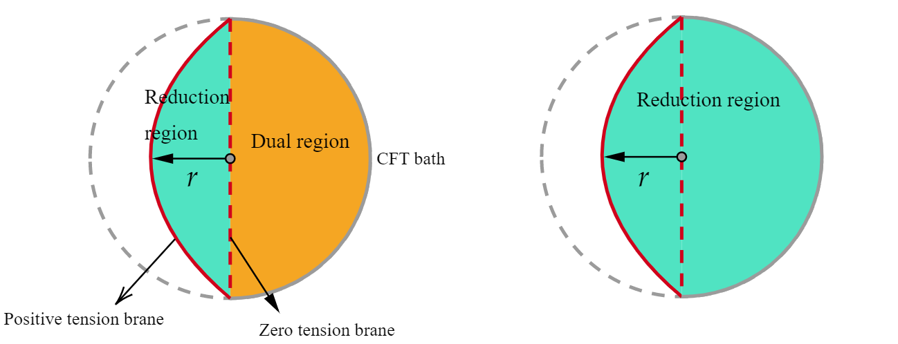
Figure 10: The illustration of partial reduction(left) and full reduction(right) of a time slice of AdS₅. The red dashed line represents the zero tension brane and red solid line is the positive tension brane.

The brane effective action includes Deng:2020ent

$$I_{eff} \supset\frac{1}{16\pi G_{N}^{(d+1)}}\left(\cosh\frac{r_{*}}{\ell}\right)^{2-d}\int_{0}^{r_{*}}dr\left(\cosh\frac{r}{\ell}\right)^{d-2}\int_{\mathrm{Q}}\sqrt{-g^{(d)}}R^{(d)}$$ (58)

$$\equiv\frac{1}{16\pi G_{N}^{(d)}}\int_{\mathrm{Q}}\sqrt{-g^{(d)}}R^{(d)}\ ,$$

where the superscript $(d)$ denotes the quantities for the effective $d$-dimensional gravity theory on the brane. One can therefore find the effective $d$-dimensional Newton constant to be

$$\frac{1}{G_{N}^{(d)}}=\frac{1}{G_{N}^{(d+1)}}\left(\cosh\frac{r_{*}}{\ell}\right)^{2-d}\int_{0}^{r_{*}}dr\left(\cosh\frac{r}{\ell}\right)^{d-2}\ .$$ (59)

In $d=4$, this gives

$$\frac{1}{G^{(4)}_{N}} =\frac{1}{G^{(5)}_{N}}\frac{1}{\cosh^{2}(r_{*}/\ell)}\int_{0}^{r_{*}}\cosh^{2}(r/\ell)dr$$ (60)

$$=\frac{1}{G^{(5)}_{N}}\frac{\left(r_{*}+\ell\sinh(r_{*}/\ell)\cosh(r_{*}/\ell)\right)}{2\cosh^{2}(r_{*}/\ell)}\ .$$

The effective Newton constant $G^{(4)}_{N}$ depends on the reduction region. In full reduction from $-\infty$ to $r_{*}$, the integration is divergent, which makes $G^{(4)}_{N}$ goes to $0$. But in partial reduction, the reduction region is from $0$ to $r_{*}$, so we obtain a finite Newton constant.

One can also discuss the partial reduction in the set up of Karch-Randall Karch:2000ct . There the brane was introduced as a delta source in the action,

$$S=\frac{1}{16\pi G_{N}^{(5)}}\left[\int d^{5}x\sqrt{|\det g_{\mu\nu}|}(R-2\Lambda_{5})+12T\int d^{4}xdr\sqrt{|\det g_{ij}|}\delta(r-r_{*})\right]\ .$$ (61)

With the coordinate transformation

$$z=\frac{1}{\sqrt{-\Lambda}}e^{\sqrt{-\Lambda}x_{3}}\ ,$$ (62)

the $5d$ metric eq. (57) becomes

$$ds^{2}=dr^{2}+\cosh^{2}\frac{r}{\ell}\cdot(-\Lambda)\ell^{2}\left[e^{-2\sqrt{-\Lambda}x_{3}}(-dt^{2}+dx_{1}^{2}+dx_{2}^{2})+dx_{3}^{2}\right]\ ,$$ (63)

where the metric in $[\,...\,]$ is a AdS₄ metric. One can check that this is indeed the solution in $r\in(0,r_{*})$ for the above action with the following ansatz

$$ds^{2}=dr^{2}+e^{2A(r)}\left[g_{ji}dx^{i}dx^{j}\right]=dr^{2}+e^{2A(r)}\left[e^{-2\sqrt{-\Lambda}x_{3}}(-dt^{2}+dx_{1}^{2}+dx_{2}^{2})+dx_{3}^{2}\right]\ .$$ (64)

The equations of motion (EOM) are

$$A^{\prime 2}-\Lambda e^{-2A}=\frac{1}{\ell^{2}}\ ,$$ (65)

$$A^{\prime\prime}+\Lambda e^{-2A}=2T\delta(r-r_{*})\ .$$ (66)

Now we calculate the perturbation of the metric to determine the spectrum following Mannheim2005Brane . Here we consider the transverse-traceless (TT) mode of the gravity fluctuations $\gamma_{ij}$ with $\nabla^{i}\gamma_{ij},\gamma_{i}^{i}=0$ and impose axial gauge $\gamma_{ir}=0$. The perturbed metric of the AdS₄ is

$$ds^{2}=dr^{2}+\left(e^{2A}g_{ij}+\gamma_{ij}\right)dx^{i}dx^{j}\ .$$ (67)

For convenience we turn to another coordinate system. Let us introduce $y=\tanh(r/\ell)$ and the EOM of $\gamma_{ij}$ becomes

$$\left[\left(1-y^{2}\right)\frac{d^{2}}{dy^{2}}-2y\frac{d}{dy}+\frac{m^{2}}{(-\Lambda)}+2-\frac{4}{\left(1-y^{2}\right)}\right]\gamma_{ij}=0\ ,$$ (68)

The mass of $4d$ graviton $m$ is defined by $4d$ wave equation

$$(\square_{4d}-2\Lambda)\gamma_{ij}=m^{2}\gamma_{ij}\ .$$ (69)

After introducing another parameter $\nu=\left(\frac{9}{4}+\frac{m^{2}}{(-\Lambda)}\right)^{1/2}-\frac{1}{2}$, eq. (68) is simplified to

$$\left[\left(1-y^{2}\right)\frac{d^{2}}{dy^{2}}-2y\frac{d}{dy}+\nu(\nu+1)-\frac{4}{\left(1-y^{2}\right)}\right]\gamma_{ij}=0\ .$$ (70)

We can decompose $\gamma_{ij}$ into $\gamma_{ij}=\epsilon_{ij}f_{m}(y)$, then the solution of this equation of motion has a general form

$$f_{m}(y)=\alpha_{m}P_{\nu}^{2}(y)+\beta_{m}Q_{\nu}^{2}(y)\ ,$$ (71)

where $P_{\nu}^{2}(y)$ and $Q_{\nu}^{2}(y)$ are the associated Legendre functions of the first and second kind. At the location of branes, we need to impose the Neumann boundary conditions,

$$\frac{1}{2}\partial_{r}\gamma_{ij}=\tanh(\frac{r}{l})\gamma_{ij}\ .$$ (72)

Substitute the general solution at $r=0$ and $r=r_{*}$, we have

$$(\nu-1)(\nu+2)\left(\alpha_{m}P_{\nu}^{1}(0)+\beta_{m}Q_{\nu}^{1}(0)\right)=0\ ,$$ (73)

$$y_{*}(\nu-1)\left(\alpha_{m}P_{\nu}^{2}(y_{*})+\beta_{m}Q_{\nu}^{2}(y_{*})\right)=(\nu-1)\left(\alpha_{m}P_{\nu+1}^{2}(y_{*})+\beta_{m}Q_{\nu+1}^{2}(y_{*})\right)\ ,$$ (74)

where $y_{*}=\tanh(\frac{r_{*}}{\ell})$. These two boundary conditions will give us the mass spectrum, and it is obvious that the solution with $\nu=1$, which is $m=0$, satisfies these boundary conditions. The solution is

$$f_{m}(y(r))=\beta_{0}Q_{1}^{2}(y(r))=\beta_{0}\frac{2}{1-y(r)^{2}}=2\beta_{0}\cosh^{2}\left({r\over\ell}\right)\ ,$$ (75)

where $\beta_{0}$ is a finite constant. For $r\in(0,r_{*})$, the zero mode is normalizable.

The EOM of $\gamma_{ij}$ can also be transformed into a Schrodinger-like equation with volcano potential Karch:2000ct . We need to rescale the perturbation $\hat{\gamma}_{ij}=\gamma_{ij}e^{-2A(r)}$ and the EOM of $\hat{\gamma}_{ij}$ is

$$\left(\partial_{r}^{2}+4A^{\prime}\partial_{r}+e^{-2A}m^{2}\right)\hat{\gamma}_{ij}=0\ .$$ (76)

Next we need to perform another coordinate transformation

$$z(r)=\frac{1}{\sqrt{-\Lambda}}\left\{\arcsin\left(\frac{1}{\cosh\left(\frac{r}{\ell}\right)}\right)-z_{0}\sqrt{-\Lambda}\right\}\ ,$$ (77)

$$z_{0}=\frac{1}{\sqrt{-\Lambda}}\arcsin\left(\frac{1}{\cosh(r_{*}/\ell)}\right)$$ (78)

and then use $H_{ij}(z)=e^{3A(z)/2}\hat{\gamma}_{ij}$, the EOM finally becomes

$$\left(-\partial_{z}^{2}+\frac{9}{4}A^{\prime}(z)^{2}+\frac{3}{2}A^{\prime\prime}(z)\right)H_{ij}(z)=m^{2}H_{ij}(z)\ .$$ (79)

The effective potential of this equation is

$$V(z) =\frac{9}{4}A^{\prime}(z)^{2}+\frac{3}{2}A^{\prime\prime}(z)$$ (80)

$$=-\frac{9}{4}(-\Lambda)+\frac{15}{4}\frac{(-\Lambda)}{\sin^{2}\left(\sqrt{-\Lambda}(z+z_{0})\right)}-3\cot\left(\sqrt{-\Lambda}z_{0}\right)\sqrt{-\Lambda}\delta(z)\ ,$$

where $z\in\left(0,\frac{\pi}{2\sqrt{-\Lambda}}-z_{0}\right)$ and we have used a delta potential. The positive tension brane locates at $z=0$ and the zero tension brane locates at $z=\frac{\pi}{2\sqrt{-\Lambda}}-z_{0}$. The potential between the positive tension brane and the zero tension brane is shown in Fig. 11. We can see that there is a potential trap at the positive tension brane, which can localize the massless graviton. The zero mode solution can be read from eq. (76) easily, which is a constant $\hat{\gamma}$. This is consistent with the solution eq. (75).

Figure 11: The volcano potential. The positive tension brane locates at $z=0$ and the reference brane locates at $z=1$. Note that there is a $\mathbb{Z}_{2}$ symmetry at $z=0$.

3.1.2 Boundary entropy in AdS/BCFT

The partial reduction can be applied in AdS₅/BCFT₄ where the BCFT₄ is defined on half of the asymptotic boundary. The EOW brane can be introduced through Neumann boundary condition. This AdS₄ brane will intersect with the asymptotic boundary and give us a boundary CFT theory as showed in Fig. 12. In Kobayashi:2018lil , the boundary entropy of this model has been calculated using on-shell action as well as RT surface. Now we review this process in the viewpoint of partial reduction and show a relation between boundary entropy and effective Newton constant. In AdS₅/BCFT₄ duality, partial reduction implies that the holographic dual of the boundary defect is the reduction region, which is the spacetime between zero tension brane and EOW brane. So the information of the boundary defect, such as boundary entropy, can be recovered from the reduction region. In Euclidean signature, the boundary entropy can be defined in terms of on-shell action

$$S_{bdy}=-I_{E}(r_{*})+\frac{1}{2}I_{E}(0)\ ,$$ (81)

where the on-shell action is

$$I_{E}(r)=-\frac{1}{16\pi G^{(5)}_{N}}\int_{-\infty}^{r_{*}}d^{5}x\sqrt{g}(R-2\Lambda_{5})-\frac{1}{8\pi G^{(5)}_{N}}\int_{Q}d^{4}y\sqrt{h}(K-(d-1)T)\ .$$ (82)

One can also view eq. (81) as the on-shell action of the reduction region. The result has been calculated in Kobayashi:2018lil

$$S_{bdy}=\frac{\ell^{3}}{4G^{(5)}_{N}}\mathrm{Vol}(\mathbb{H}^{2})\int_{0}^{r_{*}}\cosh^{2}(r/\ell)dr\ .$$ (83)

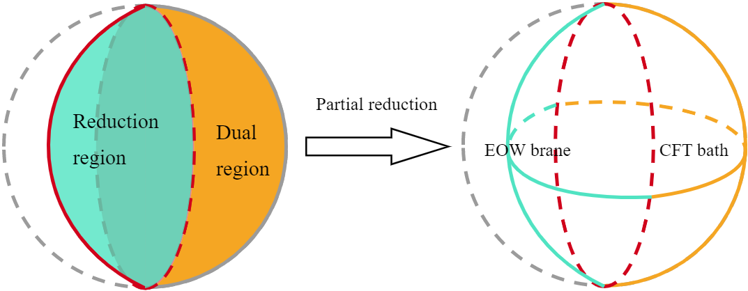
Figure 12: The partial reduction procedure of global AdS on a time slice. For AdS₅, a time slice of the BCFT₄ is defined on a $3d$ hemisphere with a S² boundary.

We can also get this result by considering an entangling surface which splits the BCFT in half. Now we turn to Lorentzian signature with metric

$$ds^{2}=dr^{2}+\cosh^{2}\left({r\over\ell}\right)(-\cosh^{2}\rho dt^{2}+d\rho^{2}+\sinh^{2}\rho d{\Omega}_{2}^{2})\ ,$$ (84)

and use

$$S_{bdy}=S^{\mathrm{BCFT}}-\frac{1}{2}S^{\mathrm{CFT}}\ ,$$ (85)

which is essentially the area of RT between the two branes as showed in Fig. 13. Note that the domain of $r$ is $(-\infty,r_{*})$. So the boundary entropy is

$$S_{bdy} =\frac{\ell^{3}}{4G^{(5)}_{N}}\mathrm{Vol}(\mathbb{H}^{2})(\int_{-\infty}^{r_{*}}\cosh^{2}(r/\ell)dr-\int_{-\infty}^{0}\cosh^{2}(r/\ell)dr)$$ (86)

$$=\frac{\ell^{3}}{4G^{(5)}_{N}}\mathrm{Vol}(\mathbb{H}^{2})\int_{0}^{r_{*}}\cosh^{2}(r/\ell)dr\ ,$$

in agreement with the on-shell action result.

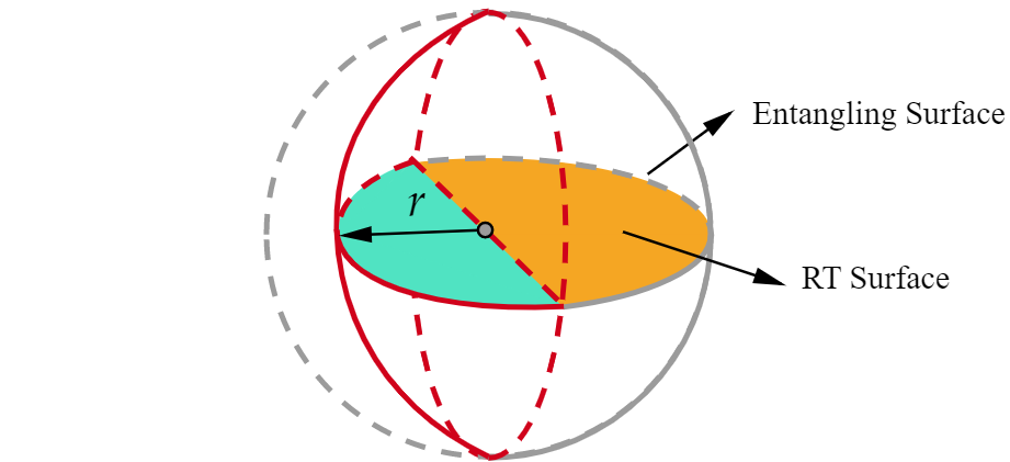
Figure 13: The colored region is the RT surface of $S^{\text{BCFT}}$. The RT of ${1\over 2}$$S^{\text{CFT}}$ corresponds to the orange region at the right side of dashed line.

Alternatively, the holographic dual of the boundary entropy can be viewed as an extremal surface between two branes. We consider an extremal surface attached freely to both the finite tension brane and the zero tension brane. Extremal condition demands orthogonal condition. This can be seen clearly in Fig. 13. We can obtain the effective Newton constant from this boundary entropy using Bekenstein-Hawking formula

$$G^{(4)}_{N} =\frac{\mathcal{A}_{4}}{4S_{bdy}} =G^{(5)}_{N}\frac{4\cosh^{2}r_{*}/\ell}{2r_{*}+\ell\sinh(2r_{*}/\ell)}\ .$$ (87)

which is the same as the result from eq. (60). Here $\mathcal{A}_{4}$ is the intersecting area of EOW brane and RT surface. Notice that the AdS radius on the brane is $\ell^{2}\cosh^{2}r_{*}/\ell$.

3.2 Partial reduction and boundary entropy for cosmology

Now let us turn to the brane model for cosmology as the $4d$ generalization of Sec. 2. For $d=4$, the bulk is an Euclidean AdS₅-Schwarzschild black hole,

$$ds^{2}=f(r)d\tau^{2}+\frac{dr^{2}}{f(r)}+r^{2}(d\theta^{2}+\sin^{2}\theta d\Omega_{2}^{2})$$ (88)

with

$$f(r)=\frac{r^{2}}{\ell^{2}}+1-\frac{r_{h}^{2}}{r^{2}}(\frac{r_{h}^{2}}{\ell^{2}}+1)\ .$$ (89)

The periodicity of the $\tau$ direction determines the temperature of the black hole, which is

$$\beta=\frac{2\pi r_{h}\ell^{2}}{\ell^{2}+2r_{h}^{2}}\ .$$ (90)

The brane trajectory $r(\tau)$ satisfies the Neumann boundary condition eq. (5) as

$$\frac{dr}{d\tau}=\pm\frac{r^{4}+r^{2}\ell^{2}-r_{h}^{2}(r_{h}^{2}+\ell^{2})}{T\ell^{2}r^{3}}\sqrt{\frac{r^{4}+r^{2}\ell^{2}-r_{h}^{2}(r_{h}^{2}+\ell^{2})}{\ell^{2}r^{2}}-T^{2}r^{2}}\ .$$ (91)

The brane trajectory is symmetric about $\tau=0$, where $r(\tau)$ takes its minimal value, which is determined by $f(r_{0})=T^{2}r_{0}^{2}$ as

$$r_{0}=\frac{1}{\sqrt{2(1-T^{2}\ell^{2})}}\left[\sqrt{\ell^{4}+4(1-T^{2}\ell^{2})r_{h}^{2}(\ell^{2}+r_{h}^{2})}-\ell^{2}\right]^{\frac{1}{2}}\ .$$ (92)

The Euclidean time $\tau_{0}$ can be obtained by subtracting half of the brane time from half of the whole time. It is related to the black hole temperature as

$$\tau_{0} =\frac{\beta}{2}-\int_{r_{0}}^{\infty}\frac{Tr}{f(r)\sqrt{f(r)-T^{2}r^{2}}}$$ (93)

$$=\frac{\pi r_{h}\ell^{2}}{\ell^{2}+2r_{h}^{2}}-\int_{r_{0}}^{\infty}\frac{Tl^{2}r^{3}}{\left[r^{4}+r^{2}\ell^{2}-r_{h}^{2}(r_{h}^{2}+\ell^{2})\right]\sqrt{\frac{r^{4}+r^{2}\ell^{2}-r_{h}^{2}(r_{h}^{2}+\ell^{2})}{\ell^{2}r^{2}}-T^{2}r^{2}}}\ .$$

Now for fixed $r_{h}$, the brane trajectory will intersect with the boundary of $(r,\tau)$ disk at different $\pm\tau_{0}$ for different tension $T$ Cooper:2018cmb . A sketch of the brane trajectory is shown in Fig. 14.

Using eq. (91) the induced metric on the brane is

$$ds^{2} =\left[f(r)+\frac{f(r)(f(r)-T^{2}r^{2})}{T^{2}r^{2}}\right]d\tau^{2}+r^{2}(d\theta^{2}+\sin^{2}\theta d\Omega_{2}^{2})$$ (94)

$$=\frac{f(r)^{2}}{T^{2}r^{2}}d\tau^{2}+r^{2}(d\theta^{2}+\sin^{2}\theta d\Omega_{2}^{2})$$

$$=d\tau_{p}^{2}+r^{2}(\tau_{p})(d\theta^{2}+\sin^{2}\theta d\Omega_{2}^{2})$$

with

$$r(\tau_{p})=\frac{1}{\sqrt{2(1-T^{2}\ell^{2})}}\left[\cosh(2\sqrt{1-T^{2}\ell^{2}}\frac{\tau_{p}}{\ell})\sqrt{\ell^{4}+4(1-T^{2}\ell^{2})r_{h}^{2}(\ell^{2}+r_{h}^{2})}-\ell^{2}\right]^{\frac{1}{2}}\ .$$ (95)

We can check that it is a hyperbolic space with scalar curvature $R_{brane}=-\frac{12(1-T^{2}\ell^{2})}{\ell^{2}}$. This metric is conformally equivalent to the finite cylinder metric $ds_{brane}^{2}=\Omega^{-2}(\tau^{\prime})ds_{cyl}^{2}=\Omega^{-2}(\tau^{\prime})(\frac{1}{\ell^{2}}d\tau^{\prime 2}+d\theta^{2}+\sin^{2}\theta d\Omega_{2}^{2})$ with a conformal factor $\Omega(\tau^{\prime})$ which we need to obtain by numerical.

Let us apply an analytical continuation to $\tau$. The time becomes $t=-i\tau$ and the brane world volume metric is

$$ds^{2} =\left[-f(r)+\frac{f(r)(T^{2}r^{2}-f(r))}{T^{2}r^{2}}\right]dt^{2}+r^{2}(d\theta^{2}+\sin^{2}\theta d\Omega_{2}^{2})$$ (96)

$$=-\frac{f(r)^{2}}{T^{2}r^{2}}dt^{2}+r^{2}(d\theta^{2}+\sin^{2}\theta d\Omega_{2}^{2})$$

$$=-dt_{p}^{2}+r^{2}(t_{p})(d\theta^{2}+\sin^{2}\theta d\Omega_{2}^{2})\ ,$$

where

$$r(t_{p})=\frac{1}{2\sqrt{(1-T^{2}\ell^{2})}}\left[\cos(2\sqrt{1-T^{2}\ell^{2}}\frac{t_{p}}{\ell})\sqrt{\ell^{4}+4(1-T^{2}\ell^{2})r_{h}^{2}(\ell^{2}+r_{h}^{2})}-\ell^{2}\right]^{\frac{1}{2}}$$ (97)

is the scale factor which describes the $4$-dim big-bang big-crunch cosmology.

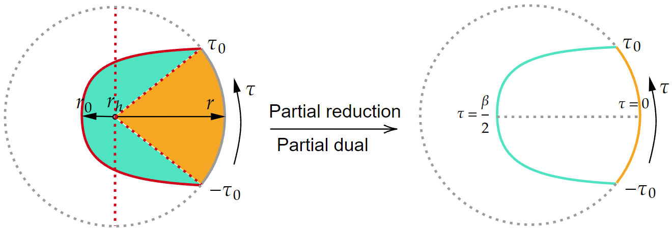
Figure 14: Partial reduction procedure for $d=4$ cosmology. The red solid line is a finite tension brane. The red dash line is the antipodal zero tension brane and the cusp zero tension brane. The orange region is dual to the boundary and the green region is reduced to the EOW brane.

In the $d=4$ cosmology model, we can find that the equation for the zero tension brane in Euclidean $(r,\tau)$ plane is given by constant $\tau$. Inspired by the pure AdS case, we choose the $\tau=\pm\tau_{0}$ zero tension brane as the reference for the partial reduction. There is a cusp in the origin, but we can regularize this cusp in a $\epsilon$ small region near the origin. This can be justified by taking the $r\to r_{h}$ first in eq. (91). The partial reduction procedure is shown in Fig. 14.

Now we calculate the boundary entropy for the Euclidean cosmology boundary state and derive the brane Newton constant. In Euclidean $(r,\tau)$ plane, similar to the brane embedded in global AdS shown in Fig. 13, the boundary entropy can be dual to an extremal surface between two branes. It can be verified that the extremal surface between the two branes is located at $\tau=0\ ,\theta=\frac{\pi}{2}$. The area of this extremal surface is

$$S_{bdy} =\frac{1}{4G_{5}}\mathrm{Vol}(\mathbb{S}^{2})\int_{r_{h}}^{r_{0}}\frac{r^{2}}{f(r)^{\frac{1}{2}}}$$ (98)

$$=\frac{1}{4G_{5}}\mathrm{Vol}(\mathbb{S}^{2})\int_{r_{h}}^{r_{0}}dr\frac{r^{2}}{\sqrt{\frac{r^{2}}{\ell^{2}}+1-\frac{r_{h}^{2}}{r^{2}}(\frac{r_{h}^{2}}{\ell^{2}}+1)}}$$

$$=\frac{1}{4G_{5}}\mathrm{Vol}(\mathbb{S}^{2})\frac{1}{2}(Tr_{0}^{2}\ell^{2}-\ell^{3}\operatorname{arcsinh}\frac{\sqrt{r_{0}^{2}-r_{h}^{2}}}{\sqrt{2r_{h}^{2}+\ell^{2}}})\ .$$

Treating this boundary entropy as an area entropy, we obtain the Newton constant given by

$$\frac{1}{4G_{4}}=\frac{S_{bdy}}{\mathrm{Vol}(\mathbb{S}^{2})r_{0}^{2}}=\frac{1}{4G_{5}}\frac{1}{2}(T\ell^{2}-{\ell^{3}\over r_{0}^{2}}\operatorname{arcsinh}\frac{\sqrt{r_{0}^{2}-r_{h}^{2}}}{\sqrt{2r_{h}^{2}+\ell^{2}}})\ .$$ (99)

Notice that there is a constrain among $T$, $r_{0}$ and $r_{h}$ in eq.(92).

One can also justify the Newton constant in Lorentzian spacetime. Let us focus on the $\tau=0$ slice which is the same as $t=0$ and compute the entanglement entropy for the equal bipartition of $\theta$ direction from two different approaches. Holographically this is given by the minimal surface between EOW brane and asymptotical boundary. On the other hand we can compute it using island formula after partial reduction. Ignoring the quantum matter located on the EOW brane, the island result is given by the sum of the Area terms and minimal surfaces between zero tension brane and asymptotical boundary. Demanding the equivalence between the two approaches, one can obtain the same Newton constant as that in Euclidean case. This is illustrated in Fig. 15. It would be very interesting to study further whether the Newton constant has a time dependence. We leave this for future work.

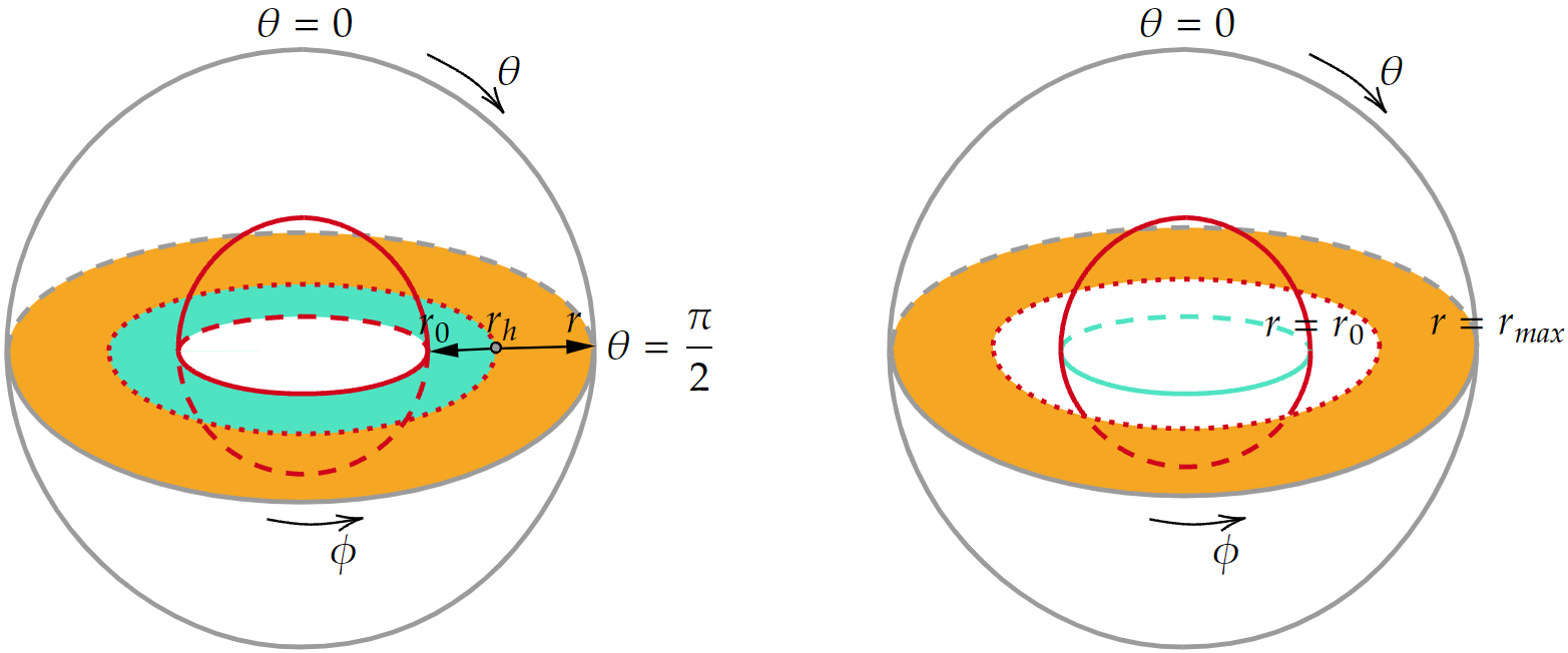
Figure 15: Left: RT surface for entangling surface at $\theta=\frac{\pi}{2}$ in $t=0$ slice. Right: after partial reduction, the boundary of island stay in $t=0$ slice with $\theta=\frac{\pi}{2}$.

4 Conclusion and discussions

We propose partial reduction as a new mechanism to localize gravity on the brane embedded in warped space. This was motivated by the recent development in information theoretical understanding of AdS_d+1/BCFT_d Deng:2020ent ; Chu:2021gdb ; Li:2021dmf . By turning on conformal matter on the brane, we have three different views of the same system: The first is AdS bulk gravity with a defect EOW brane (including the quantum matter on it); the second is the $d$-dimensional brane world gravity from partial reduction plus quantum matter on it, coupled to a CFT_d bath coming from the dual of the remaining AdS region; the third is a complicated BCFT_d with everything in the bulk encoded. These three different descriptions are equivalent. Partial reduction plays important role in clarifying the equivalence among the three different descriptions, in contrast with earlier attempts to understanding the boundary dual of Karch-Randall brane Karch:2000gx ; Aharony:2003qf , as well as the recent double holography picture Chen:2020uac ; Chen:2020hmv ; Geng:2020qvw ; Geng:2020fxl .

In this paper we focus on the application of partial reduction in cosmology. We first consider the cosmology from partial reduction in $d=2$. In particular we compute the fine grained entropy for a large subregion in CFT bath from two different approaches: One is the bulk defect extremal surface formula and the other is island formula. We compare those results and find exact agreement. We then move to $4d$ FRW cosmology where the brane trajectory is slightly complicated. We propose the proper partial reduction for the $4d$ cosmology and compute the Newton constant on the brane. We also show that partial reduction leads to a normalizable zero mode (massless graviton) on Karch-Randall brane in pure AdS₅ and suspect that the same thing will happen in $4d$ FRW cosmology.

There are a few future questions listed in order: First, extend our partial reduction mechanism to de-Sitter brane. In pure AdS₅, if one increases the brane tension beyond the critical value, the de-Sitter brane will appear Karch:2020iit and it would be interesting to study the localized gravity from partial reduction. Second, apply partial reduction to a pure Lorentzian cosmology including de-Sitter brane as well as a bath. This will tell us the fine grained entropy of a de-Sitter cosmology. Last but not least, following our construction from partial reduction, using defect and boundary CFT techniques one can try to bootstrap Collier:2021ngi ; Kusuki:2021gpt the evolutional cosmology, which will eventually open the door to simulating our observational cosmology on quantum computer.

References

- (1) G. Penington, Entanglement Wedge Reconstruction and the Information Paradox, JHEP 09 (2020) 002 [1905.08255].
- (2) A. Almheiri, N. Engelhardt, D. Marolf and H. Maxfield, The entropy of bulk quantum fields and the entanglement wedge of an evaporating black hole, JHEP 12 (2019) 063 [1905.08762].
- (3) A. Almheiri, R. Mahajan, J. Maldacena and Y. Zhao, The Page curve of Hawking radiation from semiclassical geometry, JHEP 03 (2020) 149 [1908.10996].
- (4) G. Penington, S.H. Shenker, D. Stanford and Z. Yang, Replica wormholes and the black hole interior, 1911.11977.
- (5) A. Almheiri, T. Hartman, J. Maldacena, E. Shaghoulian and A. Tajdini, Replica Wormholes and the Entropy of Hawking Radiation, JHEP 05 (2020) 013 [1911.12333].
- (6) M. Rozali, J. Sully, M. Van Raamsdonk, C. Waddell and D. Wakeham, Information radiation in BCFT models of black holes, JHEP 05 (2020) 004 [1910.12836].
- (7) F. Deng, J. Chu and Y. Zhou, Defect extremal surface as the holographic counterpart of Island formula, JHEP 03 (2021) 008 [2012.07612].
- (8) J. Chu, F. Deng and Y. Zhou, Page curve from defect extremal surface and island in higher dimensions, JHEP 10 (2021) 149 [2105.09106].
- (9) T. Takayanagi, Holographic Dual of BCFT, Phys. Rev. Lett. 107 (2011) 101602 [1105.5165].
- (10) M. Fujita, T. Takayanagi and E. Tonni, Aspects of AdS/BCFT, JHEP 11 (2011) 043 [1108.5152].
- (11) S. Cooper, M. Rozali, B. Swingle, M. Van Raamsdonk, C. Waddell and D. Wakeham, Black hole microstate cosmology, JHEP 07 (2019) 065 [1810.10601].
- (12) Y. Chen, V. Gorbenko and J. Maldacena, Bra-ket wormholes in gravitationally prepared states, JHEP 02 (2021) 009 [2007.16091].
- (13) T. Hartman, Y. Jiang and E. Shaghoulian, Islands in cosmology, JHEP 11 (2020) 111 [2008.01022].
- (14) V. Balasubramanian, A. Kar and T. Ugajin, Islands in de Sitter space, JHEP 02 (2021) 072 [2008.05275].
- (15) M. Miyaji, Island for Gravitationally Prepared State and Pseudo Entanglement Wedge, 2109.03830.
- (16) I. Kourkoulou and J. Maldacena, Pure states in the SYK model and nearly- gravity, 1707.02325.
- (17) A. Almheiri, A. Mousatov and M. Shyani, Escaping the Interiors of Pure Boundary-State Black Holes, 1803.04434.
- (18) S. Antonini and B. Swingle, Cosmology at the end of the world, Nature Phys. 16 (2020) 881 [1907.06667].
- (19) M. Van Raamsdonk, Cosmology from confinement?, 2102.05057.
- (20) S. Antonini and B. Swingle, Holographic boundary states and dimensionally-reduced braneworld spacetimes, 2105.02912.
- (21) J.L. Cardy, Boundary Conditions, Fusion Rules and the Verlinde Formula, Nucl. Phys. B 324 (1989) 581.
- (22) J.L. Cardy, Boundary conformal field theory, hep-th/0411189.
- (23) S.W. Hawking and D.N. Page, Thermodynamics of Black Holes in anti-De Sitter Space, Commun. Math. Phys. 87 (1983) 577.
- (24) E. Witten, Anti-de Sitter space, thermal phase transition, and confinement in gauge theories, Adv. Theor. Math. Phys. 2 (1998) 505 [hep-th/9803131].
- (25) J. Sully, M.V. Raamsdonk and D. Wakeham, BCFT entanglement entropy at large central charge and the black hole interior, JHEP 03 (2021) 167 [2004.13088].
- (26) M. Miyaji, T. Takayanagi and T. Ugajin, Spectrum of End of the World Branes in Holographic BCFTs, JHEP 06 (2021) 023 [2103.06893].
- (27) M. Banados, C. Teitelboim and J. Zanelli, The Black hole in three-dimensional space-time, Phys. Rev. Lett. 69 (1992) 1849 [hep-th/9204099].
- (28) T. Faulkner, A. Lewkowycz and J. Maldacena, Quantum corrections to holographic entanglement entropy, JHEP 11 (2013) 074 [1307.2892].
- (29) A. Lewkowycz and J. Maldacena, Generalized gravitational entropy, JHEP 08 (2013) 090 [1304.4926].
- (30) N. Engelhardt and A.C. Wall, Quantum Extremal Surfaces: Holographic Entanglement Entropy beyond the Classical Regime, JHEP 01 (2015) 073 [1408.3203].
- (31) S. Ryu and T. Takayanagi, Holographic derivation of entanglement entropy from AdS/CFT, Phys. Rev. Lett. 96 (2006) 181602 [hep-th/0603001].
- (32) P. Calabrese and J.L. Cardy, Entanglement entropy and quantum field theory, J. Stat. Mech. 0406 (2004) P06002 [hep-th/0405152].
- (33) A. Recknagel and V. Schomerus, Boundary Conformal Field Theory and the Worldsheet Approach to D-Branes, Cambridge Monographs on Mathematical Physics, Cambridge University Press (11, 2013), 10.1017/CBO9780511806476.
- (34) D.M. McAvity and H. Osborn, Conformal field theories near a boundary in general dimensions, Nucl. Phys. B 455 (1995) 522 [cond-mat/9505127].
- (35) T. Hartman, Entanglement Entropy at Large Central Charge, 1303.6955.
- (36) T. Faulkner, The Entanglement Renyi Entropies of Disjoint Intervals in AdS/CFT, 1303.7221.
- (37) L. Randall and R. Sundrum, A Large mass hierarchy from a small extra dimension, Phys. Rev. Lett. 83 (1999) 3370 [hep-ph/9905221].
- (38) L. Randall and R. Sundrum, An Alternative to compactification, Phys. Rev. Lett. 83 (1999) 4690 [hep-th/9906064].
- (39) I. Akal, Y. Kusuki, T. Takayanagi and Z. Wei, Codimension two holography for wedges, Phys. Rev. D 102 (2020) 126007 [2007.06800].
- (40) A. Karch and L. Randall, Locally localized gravity, JHEP 05 (2001) 008 [hep-th/0011156].
- (41) T. Li, M.-K. Yuan and Y. Zhou, Defect Extremal Surface for Reflected Entropy, 2108.08544.
- (42) P.D. Mannheim, Brane-Localized Gravity, WORLD SCIENTIFIC (2005).
- (43) N. Kobayashi, T. Nishioka, Y. Sato and K. Watanabe, Towards a -theorem in defect CFT, JHEP 01 (2019) 039 [1810.06995].
- (44) A. Karch and L. Randall, Open and closed string interpretation of SUSY CFT’s on branes with boundaries, JHEP 06 (2001) 063 [hep-th/0105132].
- (45) O. Aharony, O. DeWolfe, D.Z. Freedman and A. Karch, Defect conformal field theory and locally localized gravity, JHEP 07 (2003) 030 [hep-th/0303249].
- (46) H.Z. Chen, R.C. Myers, D. Neuenfeld, I.A. Reyes and J. Sandor, Quantum Extremal Islands Made Easy, Part I: Entanglement on the Brane, JHEP 10 (2020) 166 [2006.04851].
- (47) H.Z. Chen, R.C. Myers, D. Neuenfeld, I.A. Reyes and J. Sandor, Quantum Extremal Islands Made Easy, Part II: Black Holes on the Brane, JHEP 12 (2020) 025 [2010.00018].
- (48) H. Geng and A. Karch, Massive islands, JHEP 09 (2020) 121 [2006.02438].
- (49) H. Geng, A. Karch, C. Perez-Pardavila, S. Raju, L. Randall, M. Riojas et al., Information Transfer with a Gravitating Bath, SciPost Phys. 10 (2021) 103 [2012.04671].
- (50) A. Karch and L. Randall, Geometries with mismatched branes, JHEP 09 (2020) 166 [2006.10061].
- (51) S. Collier, D. Mazac and Y. Wang, Bootstrapping Boundaries and Branes, 2112.00750.
- (52) Y. Kusuki, Analytic Bootstrap in 2D Boundary Conformal Field Theory: Towards Braneworld Holography, 2112.10984.