An unfitted finite element method by direct extension for elliptic problems on domains with curved boundaries and interfaces

Abstract

We propose and analyze an unfitted finite element method for solving elliptic problems on domains with curved boundaries and interfaces. The approximation space on the whole domain is obtained by the direct extension of the finite element space defined on interior elements, in the sense that there is no degree of freedom locating in boundary/interface elements. The boundary/jump conditions are imposed in a weak sense in the scheme. The method is shown to be stable without any mesh adjustment or any special stabilization. Optimal convergence rates under the $L^{2}$ norm and the energy norm are derived. Numerical results in both two and three dimensions are presented to illustrate the accuracy and the robustness of the method.

keywords: elliptic problems; curved boundary; interface problems; finite element method; Nitsche’s method; unfitted mesh

1 Introduction

In recent two decades, unfitted finite element methods have become widely used tools in the numerical analysis of problems with interfaces and complex geometries [3, 4, 5, 16, 19, 28, 30, 31, 35, 36]. For such kinds of problems, the generation of the body-fitted meshes is usually a very challenging and time-consuming task, especially in three dimensions. The unfitted methods avoid the task to generate high quality meshes for representing the domain geometries accurately, due to the use of meshes independent of the interfaces and domain boundaries and the use of certain enrichment of finite element basis functions characterizing the solution singularities or discontinuities.

In [19], Hansbo and Hansbo proposed an unfitted finite element method for elliptic interface problems. The numerical solution comes from two separate linear finite element spaces and the jump conditions are weakly enforced by Nitsche’s method. This idea has been a popular discretization for interface problems and has also been applied to many other interface problems, see [10, 11, 21] and the references therein for further advances. This method can also be written into the framework of extended finite element method by a Heaviside enrichment [2, 4, 36]. We note that for penalty methods, the small cuts of the mesh have to be treated carefully, which may adversely effect the conditioning of the method and even hamper the convergence [8, 14]. In [24], Johansson and Larson proposed an unfitted high-order discontinuous Galerkin method on structured grids, where they constructed large extended elements to cure the issue of the small cuts and obtain the stability near the interface. Similar ideas of merging elements for interface problems can also be found in [8, 23, 29]. Another popular unfitted method is the cut finite element method [9], which is a variation of the extended finite element method. This method involves the ghost penalty technique [7] to guarantee the stability of the scheme. In addition, Massing and Gürkan develop a framework combining the cut finite element method and the discontinuous Galerkin method [16]. We refer to [5, 9, 12, 18, 22, 32] and the references therein for some recent applications of the cut finite element method. In [27], Lehrenfeld introduced a high order unfitted finite element method based on isoparametric mappings, where the piecewise interface is mapped approximately onto the zero level set of a high-order approximation of the level set function. We refer to [28] for an analysis of more details to this method.

In this article, we propose a new unfitted finite element method for second order elliptic problems on domains with curved boundaries and interfaces. The novelty of this method lies in that the approximation space is obtained by the direct extension of a common finite element space. We first define a standard finite element space on the set of all interior elements which are not cut by the domain boundary/interface. Then an extension operator is introduced for this space. This operator defines the polynomials on cut elements by directly extending the polynomials defined on some interior neighbouring elements. Then the approximation space is obtained from the extension operator. In the discrete schemes, a symmetric interior penalty method is adopted, and the boundary/jump conditions on the interface are weakly satisfied by Nitsche’s method. We derive optimal error estimates under the energy norm and the $L^{2}$ norm, and we give upper bounds of the condition numbers of the final linear systems. The curved boundary and the interface are allowed to intersect the mesh arbitrarily in our method. We note that the idea of associating elements that have small intersections with neighbouring interior elements can also be found in, for example, [24, 16, 23]. But different from the previous methods, the proposed method has no degrees of freedom locating in cut elements, and does not need any mesh adjustment or extra stabilization mechanism. The implementation of our method is very simple and the method can easily achieve high-order accuracy. We conduct a series of numerical experiments in two and three dimensions to illustrate the convergence behaviour.

The rest of this article is organized as follows. In Section 2, we introduce notations and prove some basic properties for the approximation space. We show the unfitted finite element method for the elliptic problem on a curved domain and the elliptic interface problem in Sections 3 and 4, respectively, and we derive optimal error estimates, and give upper bounds of the condition numbers of the discrete systems. In Section 5, we perform some numerical tests to confirm the optimal convergence rates and show the robustness of the proposed method. Finally, we make a conclusion in Section 6.

2 Preliminaries

Let $\Omega\subset\mathbb{R}^{d}(d=2,3)$ be a convex polygonal (polyhedral) domain with boundary $\partial\Omega$. Let $\Omega_{0}\Subset\Omega$ be an open subdomain with $C^{2}$-smooth or convex polygonal (polyhedral) boundary. We denote by $\Gamma:=\partial\Omega_{0}$ the topological boundary. Let $\mathcal{T}_{h}$ be a background mesh which is a quasi-uniform triangulation of the domain $\Omega$ into simplexes (see Fig. 1 for the example that $\Gamma$ is a circle). We denote by $\mathcal{E}_{h}$ the collection of all $d-1$ dimensional faces in $\mathcal{T}_{h}$. We further decompose $\mathcal{E}_{h}$ into $\mathcal{E}_{h}=\mathcal{E}_{h}^{b}\cup\mathcal{E}_{h}^{\circ}$, where $\mathcal{E}_{h}^{b}$ and $\mathcal{E}_{h}^{\circ}$ consist of boundary faces and interior faces, respectively. For any element $K\in\mathcal{T}_{h}$ and any face $e\in\mathcal{T}_{h}$, we denote by $h_{K}$ and $h_{e}$ their diameters, respectively. The mesh size $h$ is defined as $h:=\max_{K\in\mathcal{T}_{h}}h_{K}$. The quasi-uniformity of $\mathcal{T}_{h}$ is in the sense of that there exists a constant $C$ such that $h\leq C\rho_{K}$ for any element $K$, here $\rho_{K}$ is the radius of the largest ball inscribed in $K$.

Since $\Omega_{0}$ can be a curved domain, we set (see Fig. 1)

$$\mathcal{T}_{h}^{0}:=\{K\in\mathcal{T}_{h}\ |\ K\cap\Omega_{0}\neq\varnothing\},\quad\mathcal{T}_{h}^{0,\circ}:=\{K\in\mathcal{T}_{h}^{0}\ |\ K\subset\Omega_{0}\}.$$

Clearly, $\mathcal{T}_{h}^{0}$ is the minimal subset of $\mathcal{T}_{h}$ that just covers the domain $\overline{\Omega}_{0}$, and $\mathcal{T}_{h}^{0,\circ}$ is the set of elements which are inside the domain $\Omega_{0}$.

Figure 1: The background mesh $\mathcal{T}_{h}$ (left) / the mesh $\mathcal{T}_{h}^{0}$ that covers the domain $\Omega_{0}$ (right) and the elements in $\mathcal{T}_{h}^{\Gamma}$ (orange).

For the set $\mathcal{E}_{h}$, we let

$$\mathcal{E}_{h}^{0}:=\{e\in\mathcal{E}_{h}\ |\ e\cap\Omega_{0}\neq\varnothing\},\quad\mathcal{E}_{h}^{0,\circ}:=\{e\in\mathcal{E}_{h}^{0}\ |\ e\subset\Omega_{0}\}$$

be the sets of $d-1$ dimensional faces corresponding to $\mathcal{T}_{h}^{0}$ and $\mathcal{T}_{h}^{0,\circ}$, respectively. Moreover, we denote by $\mathcal{T}_{h}^{\Gamma}$ and $\mathcal{E}_{h}^{\Gamma}$ the sets of the elements and faces that are cut by $\Gamma$ (see Fig. 1), respectively:

$$\mathcal{T}_{h}^{\Gamma}:=\{K\in\mathcal{T}_{h}\ |\ K\cap\Gamma\neq\varnothing\},\quad\mathcal{E}_{h}^{\Gamma}:=\{e\in\mathcal{E}_{h}\ |\ e\cap\Gamma\neq\varnothing\}.$$

Obviously, we have $\mathcal{T}_{h}^{\Gamma}=\mathcal{T}_{h}^{0}\backslash\mathcal{T}_{h}^{0,\circ}$ and $\mathcal{E}_{h}^{\Gamma}=\mathcal{E}_{h}^{0}\backslash\mathcal{E}_{h}^{0,\circ}$. For any element $K\in\mathcal{T}_{h}^{\Gamma}$, we define the curve $\Gamma_{K}:=K\cap\Gamma$.

We make following natural geometrical assumptions on the background mesh:

Assumption 1.

For any cut face $e\in\mathcal{E}_{h}^{\Gamma}$, the intersection $e\cap\Gamma$ is simply connected; that is, $\Gamma$ does not cross a face multiple times.

Assumption 2.

For any element $K\in\mathcal{T}_{h}^{\Gamma}$, there is an element $K^{\circ}\in\Delta(K)\cap\mathcal{T}_{h}^{0,\circ}$, where $\Delta(K):=\{K^{\prime}\in\mathcal{T}_{h}\ |\ \overline{K^{\prime}}\cap\overline{K}\neq\varnothing\}$ denotes the set of elements that touch $K$.

Remark 1.

The above assumptions are widely used in interface problems [20, 32, 38], which ensure the curved boundary $\Gamma$ is well-resolved by the mesh. We note that if the mesh is fine enough, Assumptions 1 and 2 can always be fulfilled.

From the quasi-uniformity of the mesh, there exists a constant $C_{\Delta}$ independent of $h$ such that for any element $K\in\mathcal{T}_{h}$, there is a ball $B(\boldsymbol{x}_{K},C_{\Delta}h_{K})$ satisfying $\Delta(K)\subset B(\boldsymbol{x}_{K},C_{\Delta}h_{K})$, where $\boldsymbol{x}_{K}$ is the barycenter of $K$ and $B(\boldsymbol{z},r)$ denotes the ball centered at $\boldsymbol{z}$ with radius $r$. Moreover, let $\Omega^{*}$ be an open bounded domain, independent of the mesh size $h$ and $\Gamma$, which includes the union of all balls $B(\boldsymbol{x}_{K},C_{\Delta}h_{K})$ $(\forall K\in\mathcal{T}_{h})$, that is, $B(\boldsymbol{x}_{K},C_{\Delta}h_{K})\in\Omega^{*}$ for any $K\in\mathcal{T}_{h}$.

Next, we introduce the jump and average operators which are widely used in the discontinuous Galerkin framework. Let $e\in\mathcal{E}_{h}^{\circ}$ be any interior face shared by two neighbouring elements $K^{+}$ and $K^{-}$, with the unit outward normal vectors $\boldsymbol{\mathrm{n}}^{+}$ and $\boldsymbol{\mathrm{n}}^{-}$ along $e$, respectively. For any piecewise smooth scalar-valued function $v$ and piecewise smooth vector-valued function $\boldsymbol{q}$, the jump operator $[[\cdot]]$ is defined as

$$[[v]]|_{e}:=(v|_{K^{+}})|_{e}\boldsymbol{\mathrm{n}}^{+}+(v|_{K^{-}})|_{e}\boldsymbol{\mathrm{n}}^{-},\quad[[\boldsymbol{q}]]|_{e}:=(\boldsymbol{q}|_{K^{+}})|_{e}\cdot\boldsymbol{\mathrm{n}}^{+}+(\boldsymbol{q}|_{K^{-}})|_{e}\cdot\boldsymbol{\mathrm{n}}^{-},$$

and the average operator $\{\cdot\}$ is defined as

$$\{v\}|_{e}:=\frac{1}{2}\left((v|_{K^{+}})|_{e}+(v|_{K^{-}})|_{e}\right),\quad\{\boldsymbol{q}\}|_{e}:=\frac{1}{2}\left((\boldsymbol{q}|_{K^{+}})|_{e}+(\boldsymbol{q}|_{K^{-}})|_{e}\right).$$

On a boundary face $e\in\mathcal{E}_{h}^{b}$ with the unit outward normal vector $\boldsymbol{\mathrm{n}}$, we define

$$\{v\}|_{e}:=v|_{e},\quad[[v]]|_{e}:=v|_{e}\boldsymbol{\mathrm{n}},\quad\{\boldsymbol{q}\}|_{e}:=\boldsymbol{q}|_{e},\quad[[\boldsymbol{q}]]|_{e}:=\boldsymbol{q}|_{e}\cdot\boldsymbol{\mathrm{n}}.$$

We will also employ the jump operator $[[\cdot]]$ and the average $\{\cdot\}$ on $\Gamma$, that is,

$$[[v]]|_{\Gamma},\quad\{v\}|_{\Gamma},\quad[[\boldsymbol{q}]]|_{\Gamma},\quad\{\boldsymbol{q}\}|_{\Gamma},$$ (1)

and their definitions will be given later for specific problems.

Throughout this paper, we denote by $C$ and $C$ with subscripts the generic positive constants that may vary between lines but are independent of the mesh size $h$ and how $\Gamma$ cuts the mesh $\mathcal{T}_{h}$. For a bounded domain $D$, we follow the standard notations of the Sobolev spaces $L^{2}(D)$, $H^{r}(D)(r\geq 0)$ and their corresponding inner products, norms and semi-norms. For the partition $\mathcal{T}_{h}$, the notations of broken Sobolev spaces $L^{2}(\mathcal{T}_{h})$, $H^{1}(\mathcal{T}_{h})$ are also used as well as their associated inner products and broken Sobolev norms.

We follow three steps to give the definition of the approximation space $V_{h,0}^{m}$ with respect to the partition $\mathcal{T}_{h}^{0}$.

Step 1. Let $V_{h,0}^{m,\circ}$ be the space of piecewise polynomials of degree $m\geq 1$ on $\mathcal{T}_{h}^{0,\circ}$. Here $V_{h,0}^{m,\circ}$ can be the standard $C^{0}$ finite element space or the discontinuous finite element space, i.e.

$$V_{h,0}^{m,\circ}=\{v_{h}\in C(\mathcal{T}_{h}^{0,\circ})\ |\ v_{h}|_{K}\in\mathbb{P}_{m}(K),\ \forall K\in\mathcal{T}_{h}^{0,\circ}\},$$

or

$$V_{h,0}^{m,\circ}=\{v_{h}\in L^{2}(\mathcal{T}_{h}^{0,\circ})\ |\ v_{h}|_{K}\in\mathbb{P}_{m}(K),\ \forall K\in\mathcal{T}_{h}^{0,\circ}\},$$

where $\mathbb{P}_{m}(K)$ denotes the set of polynomials of degree $m$ defined on $K$.

Step 2. We extend the space $V_{h,0}^{m,\circ}$ to the mesh $\mathcal{T}_{h}^{0}$ by introducing an extension operator $E_{h,0}$. To this end, for every element $K\in\mathcal{T}_{h}$, we define a local extension operator

$$\begin{aligned} E_{K}:\mathbb{P}_{m}(K)&\rightarrow\mathbb{P}_{m}(B(\boldsymbol{x}_{K},C_{\Delta}h_{K})),\\ v&\mapsto E_{K}v,\\ \end{aligned}\quad v|_{K}=(E_{K}v)|_{K}.$$ (2)

For any $v\in\mathbb{P}_{m}(K)$, $E_{K}v$ is a polynomial defined on the ball $B(\boldsymbol{x}_{K},C_{\Delta}h_{K})$ and has the same expression as $v$. Then the operator $E_{h,0}$ is defined in a piecewise manner: for any $K\in\mathcal{T}_{h}^{0}$ and $v_{h}\in V_{h,0}^{m,\circ}$,

$$(E_{h,0}v_{h})|_{K}:=\begin{cases}v_{h}|_{K},&\forall K\in\mathcal{T}_{h}^{0,\circ},\\ (E_{K^{\circ}}v)|_{K},&\forall K\in\mathcal{T}_{h}^{\Gamma},\\ \end{cases}$$ (3)

where $K^{\circ}$ is defined in Assumption 2. Note that for any cut element $K\in\mathcal{T}_{h}^{\Gamma}$, the operator $E_{h,0}$ extends polynomials of degree $m$ from the assigned interior element $K^{\circ}$ to $K$.

Step 3. We define the approximation space $V_{h,0}^{m}$ as the image space of the operator $E_{h,0}$,

$$V_{h,0}^{m}:=\{E_{h,0}v_{h}\ |\ \forall v_{h}\in V_{h,0}^{m,\circ}\}.$$

From (3), it can be seen that $V_{h,0}^{m}$ is a piecewise polynomial space and shares the same degrees of freedom of the space $V_{h,0}^{m,\circ}$, which implies that all degrees of freedom of $V_{h,0}^{m}$ locate inside the domain $\Omega_{0}$.

Let $I_{h,0}$ be the corresponding Lagrange interpolation operator of the space $V_{h,0}^{m,\circ}$ and recall that $\Omega^{*}$ is an open bounded domain including the union of all balls $B(\boldsymbol{x}_{K},C_{\Delta}h_{K})$ $(\forall K\in\mathcal{T}_{h})$. Then the following lemma shows the approximation property of the space $V_{h,0}^{m}$.

Lemma 1.

For any element $K\in\mathcal{T}_{h}^{0,\circ}$, there exists a constant $C$ such that

$$\|u-I_{h,0}u\|_{H^{q}(K)}\leq Ch_{K}^{m+1-q}\|u\|_{H^{m+1}(K)},\quad q=0,1,\quad\forall u\in H^{m+1}(\Omega^{*}),$$ (4)

and for any element $K\in\mathcal{T}_{h}^{\Gamma}$, there exists a constant $C$ such that

$$\|u-E_{h,0}(I_{h,0}u)\|_{H^{q}(K)}\leq Ch_{K}^{m+1-q}\|u\|_{H^{m+1}(B(\boldsymbol{x}_{K^{\circ}},C_{\Delta}h_{K^{\circ}}))},\quad q=0,1,\quad\forall u\in H^{m+1}(\Omega^{*}).$$ (5)

Proof.

It is sufficient to verify the estimate (5), since the estimate (4) is standard. For the ball $B(\boldsymbol{x}_{K^{\circ}},C_{\Delta}h_{K^{\circ}})$, there exists a polynomial $v_{h}\in\mathbb{P}_{m}(B(\boldsymbol{x}_{K^{\circ}},C_{\Delta}h_{K^{\circ}}))$ such that [6]

$$\|u-v_{h}\|_{H^{q}(B(\boldsymbol{x}_{K^{\circ}},C_{\Delta}h_{K^{\circ}}))}\leq Ch_{K^{\circ}}^{m+1-q}\|u\|_{H^{m+1}(B(\boldsymbol{x}_{K^{\circ}},C_{\Delta}h_{K^{\circ}}))}.$$

Thus, we have that

$$\|u-E_{h,0}(I_{h,0}u)\|_{H^{q}(K)}\leq\|u-v_{h}\|_{H^{q}(K)}+\|v_{h}-E_{h,0}(I_{h,0}u)\|_{H^{q}(K)}.$$

From the mesh regularity, there exists a constant $C_{1}$ such that

$$C_{\Delta}\leq(C_{\Delta}h_{K^{\circ}})/\rho_{K^{\circ}}\leq C_{1}.$$

Considering the norm equivalence between $\|\cdot\|_{L^{2}(B(\boldsymbol{x}_{K^{\circ}},C_{1}))}$ and $\|\cdot\|_{L^{2}(B(\boldsymbol{x}_{K^{\circ}},1))}$ for the space $\mathbb{P}_{m}(\cdot)$ and the affine mapping from $B(\boldsymbol{x}_{K^{\circ}},1)$ to the $B(\boldsymbol{x}_{K^{\circ}},\rho_{K^{\circ}})$, there holds

$$\|q_{h}\|_{H^{q}(B(\boldsymbol{x}_{K^{\circ}},C_{\Delta}h_{K^{\circ}}))}\leq C\|q_{h}\|_{H^{q}(B(\boldsymbol{x}_{K^{\circ}},\rho_{K^{\circ}}))},\quad\forall q_{h}\in\mathbb{P}_{m}(B(\boldsymbol{x}_{K^{\circ}},C_{\Delta}h_{K^{\circ}})).$$

Combining $h_{K^{\circ}}\leq Ch_{K}$, the above result brings us that

$$\|v_{h}-E_{h,0}(I_{h,0}u)\|_{H^{q}(K)} =\|E_{h,0}(v_{h}-I_{h,0}u)\|_{H^{q}(K)}\leq\|E_{h,0}(v_{h}-I_{h,0}u)\|_{H^{q}(B(\boldsymbol{x}_{K^{\circ}},Ch_{K^{\circ}}))}$$

$$\leq C\|v_{h}-I_{h,0}u\|_{H^{q}(B(\boldsymbol{x}_{K^{\circ}},\rho_{K^{\circ}}))}\leq C\|v_{h}-I_{h,0}u\|_{H^{q}(K^{\circ})}$$

$$\leq C\left(\|u-v_{h}\|_{H^{q}(K^{\circ})}+\|u-I_{h,0}u\|_{H^{q}(K^{\circ})}\right)$$

$$\leq Ch_{K}^{m+1-q}\|u\|_{H^{m+1}(B(\boldsymbol{x}_{K^{\circ}},Ch_{K^{\circ}}))},$$

which completes the proof. ∎

We have given the definition and the basic property of the approximation space. The implementation of the space is the same as the common finite element spaces, which is very simple and does not need any strategy for adjusting the mesh to eliminate the effects of the small cuts. Thus the curve $\Gamma$ is allowed to intersect the partition in an arbitrary fashion. In next two sections, we will apply the space $V_{h,0}^{m}$ to solve the elliptic problem on a curved domain and the elliptic interface problem, respectively.

3 Approximation to Elliptic Problem on Curved Domain

In this section, we are concerned with the model boundary problem defined on the curved domain $\Omega_{0}$: seek $u$ such that

$$-\Delta u =f, \text{in }\Omega_{0},$$ (6)

$$u =g, \text{on }\Gamma.$$

We assume $f\in L^{2}(\Omega_{0})$ and $g\in H^{3/2}(\Gamma)$. Then the problem (6) admits a unique solution $u\in H^{2}(\Omega_{0})$ from the standard regularity result [15].

For this problem, the mesh $\mathcal{T}_{h}$ can be regarded as a background mesh that entirely covers the domain $\overline{\Omega}_{0}$, and $\mathcal{T}_{h}^{0}$ is the minimal subsets of $\mathcal{T}_{h}$ covering $\Omega_{0}$. The trace operators in (1) for this problem are specified as

$$\{v\}|_{\Gamma_{K}}:=v|_{\Gamma_{K}},\quad[[v]]|_{\Gamma_{K}}:=v|_{\Gamma_{K}}\boldsymbol{\mathrm{n}},\quad\{\boldsymbol{q}\}|_{\Gamma_{K}}:=\boldsymbol{q}|_{\Gamma_{K}},\quad[[\boldsymbol{q}]]|_{\Gamma_{K}}:=\boldsymbol{q}|_{\Gamma_{K}}\cdot\boldsymbol{\mathrm{n}},$$

for any $K\in\mathcal{T}_{h}^{\Gamma}$, where $\boldsymbol{\mathrm{n}}$ denotes the unit outward normal vector on $\Gamma$.

We solve the problem (6) by the space $V_{h,0}^{m}$, and the numerical solution is sought by the following discrete variational form: find $u_{h}\in V_{h,0}^{m}$ such that

$$a_{h}(u_{h},v_{h})=l_{h}(v_{h}),\quad\forall v_{h}\in V_{h,0}^{m},$$ (7)

where the bilinear form $a_{h}(\cdot,\cdot)$ takes the form

$$a_{h}(u_{h},v_{h}) := \sum_{K\in\mathcal{T}_{h}^{0}}\int_{K\cap\Omega_{0}}\nabla u_{h}\cdot\nabla v_{h}\mathrm{d}\boldsymbol{x}$$

$$-\sum_{e\in\mathcal{E}_{h}^{0}}\int_{e\cap\Omega_{0}}\left(\{\nabla u_{h}\}\cdot[[v_{h}]]{+}\{\nabla v_{h}\}\cdot[[u_{h}]]{-}\frac{\mu}{h_{e}}[[u_{h}]]\cdot[[v_{h}]]\right)d{s}$$

$$-\sum_{K\in\mathcal{T}_{h}^{\Gamma}}\int_{\Gamma_{K}}\left(\{\nabla u_{h}\}\cdot[[v_{h}]]{+}\{\nabla v_{h}\}\cdot[[u_{h}]]{-}\frac{\mu}{h_{K}}[[u_{h}]]\cdot[[v_{h}]]\right)d{s},$$

where $\mu$ is the positive penalty parameter and will be specified later on. The linear form $l_{h}(\cdot)$ reads

$$l_{h}(v_{h}):=\sum_{K\in\mathcal{T}_{h}^{0}}\int_{K\cap\Omega_{0}}fv_{h}d{x}-\sum_{K\in\mathcal{T}_{h}^{\Gamma}}\int_{\Gamma_{K}}\{\nabla v_{h}\}\cdot\boldsymbol{\mathrm{n}}{g}\mathrm{d}\boldsymbol{s}+\sum_{K\in\mathcal{T}_{h}^{\Gamma}}\int_{\Gamma_{K}}\frac{\mu}{h_{K}}[[v_{h}]]\cdot\boldsymbol{\mathrm{n}}g\mathrm{d}\boldsymbol{s}.$$ (9)

Notice that (3) is suitable for both cases that $V_{h,0}^{m,\circ}$ is the discontinuous piecewise polynomial space or the $C^{0}$ finite element space. If $V_{h,0}^{m,\circ}$ is chosen to be the continuous space, $a_{h}(\cdot,\cdot)$ can be further simplified, see Remark 2.

Remark 2.

For the $C^{0}$ finite element space $V_{h,0}^{m,\circ}$, the terms defined on $\mathcal{E}_{h}^{0}$

$$\sum_{e\in\mathcal{E}_{h}^{0}}\int_{e\cap\Omega_{0}}\{\nabla u_{h}\}\cdot[[v_{h}]]\mathrm{d}\boldsymbol{s},\quad\sum_{e\in\mathcal{E}_{h}^{0}}\int_{e\cap\Omega_{0}}\{\nabla v_{h}\}\cdot[[u_{h}]]\mathrm{d}\boldsymbol{s},\quad\sum_{e\in\mathcal{E}_{h}^{0}}\int_{e\cap\Omega_{0}}\mu h_{e}^{-1}[[u_{h}]]\cdot[[v_{h}]]\mathrm{d}\boldsymbol{s},$$

are reduced to

$$\sum_{e\in\mathcal{E}_{h}^{\Gamma}}\int_{e\cap\Omega_{0}}\{\nabla u_{h}\}\cdot[[v_{h}]]\mathrm{d}\boldsymbol{s},\quad\sum_{e\in\mathcal{E}_{h}^{\Gamma}}\int_{e\cap\Omega_{0}}\{\nabla v_{h}\}\cdot[[u_{h}]]\mathrm{d}\boldsymbol{s},\quad\sum_{e\in\mathcal{E}_{h}^{\Gamma}}\int_{e\cap\Omega_{0}}\mu h_{e}^{-1}[[u_{h}]]\cdot[[v_{h}]]\mathrm{d}\boldsymbol{s},$$

respectively.

Remark 3.

The scheme (7) can be termed as a symmetric interior penalty finite element method since $a_{h}(v_{h},w_{h})=a_{h}(w_{h},v_{h})$. In fact, if we replace the trace terms

$$\int_{e\cap\Omega_{0}}\{\nabla v_{h}\}\cdot[[u_{h}]]\mathrm{d}\boldsymbol{s}\ \text{ and }\ \int_{\Gamma_{K}}\{\nabla v_{h}\}\cdot[[u_{h}]]\mathrm{d}\boldsymbol{s}$$

in (3) with

$$\int_{e\cap\Omega_{0}}-\{\nabla v_{h}\}\cdot[[u_{h}]]\mathrm{d}\boldsymbol{s}\ \text{ and }\ \int_{\Gamma_{K}}-\{\nabla v_{h}\}\cdot[[u_{h}]]\mathrm{d}\boldsymbol{s},$$

respectively, then the modified scheme corresponds to a non-symmetric interior penalty method [33]. The analysis for the error estimate (18) under the energy norm can be easily adapted for this case. Particularly, the non-symmetric method has a parameter-friendly feature, i.e. $\mu$ can be selected as any positive number.

Next, we focus on the well-posedness of the discrete problem (7). For this goal, we introduce an energy norm $\|\cdot\|_{{\mathrm{DG}}}$ defined by

$$\|v_{h}\|_{{\mathrm{DG}}}^{2}:=\sum_{K\in\mathcal{T}_{h}^{0}}\|\nabla v_{h} \|_{L^{2}(K\cap\Omega_{0})}^{2}+\sum_{e\in\mathcal{E}_{h}^{0}}h_{e}\|\{\nabla v_{h}\}\|_{L^{2}(e\cap\Omega_{0})}^{2}+\sum_{e\in\mathcal{E}_{h}^{0}}h_{e}^{-1}\|[[v_{h}]]\|_{L^{2}(e\cap\Omega_{0})}^{2}$$

$$+ \sum_{K\in\mathcal{T}_{h}^{\Gamma}}h_{K}\|\{\nabla v_{h}\}\|_{L^{2}(\Gamma_{K})}^{2}+\sum_{K\in\mathcal{T}_{h}^{\Gamma}}h_{K}^{-1}\|[[v_{h}]]\|_{L^{2}(\Gamma_{K})}^{2},$$

for any $v_{h}\in V_{h,0}:=V_{h,0}^{m}+H^{2}(\Omega_{0})$.

We give the following discrete trace estimate and inverse estimate on $\Gamma$, which are crucial in the forthcoming analysis.

Lemma 2.

There exists a constant $C$ such that for any $K\in\mathcal{T}_{h}^{\Gamma}$ and $\alpha=0,1$, it holds

$$\|D^{\alpha}v_{h}\|_{L^{2}((\partial K)^{0})}\leq Ch_{K}^{-1/2}\|D^{\alpha}v_{h}\|_{L^{2}(K^{\circ})},\quad\forall v_{h}\in V_{h,0}^{m},$$ (10)

$$\|D^{\alpha}v_{h}\|_{L^{2}(K\cap\Omega_{0})}\leq C\|D^{\alpha}v_{h}\|_{L^{2}(K^{\circ})},\quad\forall v_{h}\in V_{h,0}^{m},$$ (11)

where $(\partial K)^{0}=(\partial K\cap\Omega_{0})\cup\Gamma_{K}$.

Proof.

Clearly, $(\partial K)^{0}\in B(\boldsymbol{x}_{K^{\circ}},C_{\Delta}h_{K^{\circ}})$ and the ball $B(\boldsymbol{x}_{K^{\circ}},\rho_{K^{\circ}})\in K^{\circ}$. By (3), $(D^{\alpha}v_{h})|_{(\partial K)^{0}}$ has the same expression as $(D^{\alpha}v_{h})|_{K^{\circ}}$, and we deduce that

$$\|D^{\alpha}v_{h}\|_{L^{2}((\partial K)^{0})} \leq|(\partial K)^{0}|^{1/2}\|D^{\alpha}v_{h}\|_{L^{\infty}(B(\boldsymbol{x}_{K^{\circ}},C_{\Delta}h_{K^{\circ}}))}$$

$$\leq C|(\partial K)^{0}|^{1/2}|B(\boldsymbol{x}_{K^{\circ}},C_{\Delta}h_{K^{\circ}})|^{-1/2}\|D^{\alpha}v_{h}\|_{L^{2}(B(\boldsymbol{x}_{K^{\circ}},\rho_{K^{\circ}}))}$$

$$\leq C|(\partial K)^{0}|^{1/2}|B(\boldsymbol{x}_{K^{\circ}},C_{\Delta}h_{K^{\circ}})|^{-1/2}\|D^{\alpha}v_{h}\|_{L^{2}(K^{\circ})}$$

$$\leq Ch_{K}^{-1/2}\|D^{\alpha}v_{h}\|_{L^{2}(K^{\circ})},$$

where in the second inequality we have used the mesh regularity $C_{\Delta}h_{K}/\rho_{K}\leq C$ and a scaling argument that applies the inverse inequality $\|q_{h}\|_{L^{\infty}(B(0,1))}\leq C\|q_{h}\|_{L^{2}(B(0,\rho_{K}/(C_{\Delta}h_{K})))}$ for any $q_{h}\in\mathbb{P}_{m}(B(0,1))$ and the pullback with the bijective affine map from the ball $B(\boldsymbol{x}_{K^{\circ}},C_{\Delta}h_{K^{\circ}})$ to $B(0,1)$, and in the last inequality, we have used the mesh regularity $C_{1}h_{K}\leq h_{K^{\circ}}\leq C_{2}h_{K}$ and the estimate $|(\partial K)^{0}|\leq Ch_{K}^{d-1}$ [38] due to the fact that $\Gamma$ is $C^{2}$-smooth or polygonal. Thus the estimate (10) holds.

Similarly, we can obtain the estimate (11). This completes the proof. ∎

Based on above results, we are ready to prove that the bilinear form $a_{h}(\cdot,\cdot)$ is bounded and coercive under the energy norm $\|\cdot\|_{{\mathrm{DG}}}$.

Lemma 3.

Let $a_{h}(\cdot,\cdot)$ be defined as (3), there exists a constant $C$ such that

$$|a_{h}(u_{h},v_{h})|\leq C\|u_{h}\|_{{\mathrm{DG}}}\|v_{h}\|_{{\mathrm{DG}}},\quad\forall u_{h},v_{h}\in{V_{h,0}},$$ (12)

and with a sufficiently large $\mu$, there exists a constant $C$ such that

$$a_{h}(v_{h},v_{h})\geq C\|v_{h}\|_{{\mathrm{DG}}}^{2},\quad\forall v_{h}\in V_{h,0}^{m}.$$ (13)

Proof.

By Cauchy-Schwarz inequality, we directly have

$$-2\int_{e\cap\Omega_{0}}\{\nabla u_{h}\}\cdot[[v_{h}]]\mathrm{d}\boldsymbol{s}\leq h_{e}\|\{\nabla u_{h}\}\|_{L^{2}(e\cap\Omega_{0})}+h_{e}^{-1}\|[[v_{h}]]\|_{L^{2}(e\cap\Omega_{0})}.$$

The other terms in (3) can be bounded analogously. Thus, the boundedness (12) follows from the definition of $\|\cdot\|_{{\mathrm{DG}}}$.

The rest is to prove the coercivity (13). We introduce a weaker norm $\|\cdot\|_{*}$, which is more natural for analysis,

$$\|w_{h}\|_{*}^{2}:=\sum_{K\in\mathcal{T}_{h}^{0}}\|\nabla w_{h}\|_{L^{2}(K\cap\Omega_{0})}^{2}+\sum_{e\in\mathcal{E}_{h}^{0}}h_{e}^{-1}\|[[w_{h}]]\|_{L^{2}(e\cap\Omega_{0})}^{2}+\sum_{K\in\mathcal{T}_{h}^{\Gamma}}h_{K}^{-1}\|[[w_{h}]]\|_{L^{2}(\Gamma_{K})}^{2},$$

for $\forall w_{h}\in V_{h,0}^{m}$. Then we state the equivalence between the norm $\|\cdot\|_{{\mathrm{DG}}}$ and the weaker norm $\|\cdot\|_{*}$ restricted on the approximation space $V_{h,0}^{m}$. Obviously, it suffices to prove $\|w_{h}\|_{{\mathrm{DG}}}\leq C\|w_{h}\|_{*}$. To this end, we are required to bound the summation $\sum_{e\in\mathcal{E}_{h}^{0}}h_{e}\|\{\nabla w_{h}\}\|_{L^{2}(e\cap\Omega_{0})}^{2}$ and $\sum_{K\in\mathcal{T}_{h}^{\Gamma}}h_{K}\|\{\nabla w_{h}\}\|_{L^{2}(\Gamma_{K})}^{2}$ of $\|w_{h}\|_{{\mathrm{DG}}}$. By the trace estimate (10), we obtain that

$$\sum_{K\in\mathcal{T}_{h}^{\Gamma}}h_{K}\|\{\nabla w_{h}\}\|_{L^{2}(\Gamma_{K})}^{2} \leq\sum_{K\in\mathcal{T}_{h}^{\Gamma}}C\|\nabla w_{h}\|_{L^{2}(K^{\circ})}^{2}\leq C\sum_{K\in\mathcal{T}_{h}^{0}}\|\nabla w_{h}\|_{L^{2}(K\cap\Omega_{0})}^{2}$$

$$\leq C\|w_{h}\|_{*}^{2}.$$

Further, we consider the trace term defined on $e\in\mathcal{E}_{h}^{0}$. Let $e$ be shared by two neighbouring elements $K_{1}$ and $K_{2}$, we deduce that

$$h_{e}\|\{\nabla w_{h}\}\|_{L^{2}(e\cap\Omega_{0})}^{2} \leq Ch_{e}\left(\|\nabla w_{h}\|_{L^{2}(\partial K_{1}\cap\Omega_{0})}^{2}+\|\nabla w_{h}\|_{L^{2}(\partial K_{2}\cap\Omega_{0})}^{2}\right)$$

$$\leq Ch_{K_{1}}\|\nabla w_{h}\|_{L^{2}(\partial K_{1}\cap\Omega_{0})}^{2}+Ch_{K_{2}}\|\nabla w_{h}\|_{L^{2}(\partial K_{2}\cap\Omega_{0})}^{2}.$$

If $K_{i}\in\mathcal{T}_{h}^{\Gamma}(i=1\ \text{or}\ 2)$ is a cut element, from the trace inequality (10), there holds

$$h_{K_{i}}\|\nabla w_{h}\|_{L^{2}(\partial K_{i}\cap\Omega_{0})}^{2}\leq C\|\nabla w_{h}\|_{L^{2}((K_{i})^{\circ})}^{2}.$$

If $K_{i}\in\mathcal{T}_{h}^{0,\circ}$ is a non-interface element, the standard trace estimate directly gives that

$$h_{K_{i}}\|\nabla w_{h}\|_{L^{2}(\partial K_{i}\cap\Omega_{0})}^{2}\leq C\|\nabla w_{h}\|_{L^{2}(K_{i})}^{2}.$$

Combining the above estimates shows that

$$\sum_{e\in\mathcal{E}_{h}^{0}}h_{e}\|\{\nabla w_{h}\}\|_{L^{2}(e\cap\Omega_{0})}^{2}\leq C\sum_{K\in\mathcal{T}_{h}^{0}}\|\nabla w_{h}\|_{L^{2}(K\cap\Omega_{0})}^{2}\leq C\|w_{h}\|_{*}^{2},$$ (14)

which implies $\|w_{h}\|_{{\mathrm{DG}}}\leq C\|w_{h}\|_{*}$, and also the equivalence between $\|\cdot\|_{*}$ and $\|\cdot\|_{{\mathrm{DG}}}$. This fact inspires us to prove the coercivity under the norm $\|\cdot\|_{*}$. From the Cauchy-Schwarz inequality and the estimate (14), for any $\varepsilon>0$ there holds

$$-2\sum_{e\in\mathcal{E}_{h}^{0}}\int_{e\cap\Omega_{0}}\{\nabla v_{h}\}\cdot[[v_{h}]]\mathrm{d}\boldsymbol{s} \geq-\sum_{e\in\mathcal{E}_{h}^{0}}\varepsilon h_{e}\|\{\nabla v_{h}\}\|_{L^{2}(e\cap\Omega_{0})}^{2}-\sum_{e\in\mathcal{E}_{h}^{0}}\varepsilon^{-1}h_{e}^{-1}\|[[v_{h}]]\|_{L^{2}(e\cap\Omega_{0})}^{2}$$

$$\geq-C\varepsilon\sum_{K\in\mathcal{T}_{h}^{0}}\|\nabla v_{h}\|_{L^{2}(K\cap\Omega_{0})}^{2}-\sum_{e\in\mathcal{E}_{h}^{0}}\varepsilon^{-1}h_{e}^{-1}\|[[v_{h}]]\|_{L^{2}(e\cap\Omega_{0})}^{2}.$$

The terms defined on $\Gamma_{K}$ can be bounded similarly, i.e.

$$-2\sum_{K\in\mathcal{T}_{h}^{\Gamma}}\int_{\Gamma_{K}}\{\nabla v_{h}\}\cdot[[v_{h}]]\mathrm{d}\boldsymbol{s}\geq-C\varepsilon\sum_{K\in\mathcal{T}_{h}^{0}}\|\nabla v_{h}\|_{L^{2}(K\cap\Omega_{0})}^{2}-\sum_{K\in\mathcal{T}_{h}^{\Gamma}}\varepsilon^{-1}h_{K}^{-1}\|[[v_{h}]]\|_{L^{2}(\Gamma_{K})}^{2}.$$

By collecting all above results, we conclude that there exist constants $C_{1}$, $C_{2}$ and $C_{3}$ such that for any $\varepsilon>0$ there holds

$$a_{h}(v_{h},v_{h})\geq(1-\varepsilon C_{1})\sum_{K\in\mathcal{T}_{h}^{0}}\|\nabla v_{h} \|_{L^{2}(K\cap\Omega_{0})}^{2}+(\mu-C_{2}/\varepsilon)\sum_{e\in\mathcal{E}_{h}^{0}}h_{e}^{-1}\|[[v_{h}]]\|_{L^{2}(e\cap\Omega_{0})}^{2}$$

$$+(\mu-C_{3}/\varepsilon)\sum_{K\in\mathcal{T}_{h}^{\Gamma}}h_{K}^{-1}\|[[v_{h}]]\|_{L^{2}(\Gamma_{K})}^{2}.$$

Choose $\varepsilon=1/(2C_{1})$ and take a sufficiently large $\mu$, we arrive at $a_{h}(v_{h},v_{h})\geq C\|v_{h}\|_{*}^{2}$, which gives the estimate (13) and completes the proof. ∎

The Galerkin orthogonality also holds for the bilinear form $a_{h}(\cdot,\cdot)$ and $l_{h}(\cdot)$.

Lemma 4.

Let $u\in H^{2}(\Omega)$ be the exact solution to problem (6), and let $u_{h}\in V_{h}^{m}$ be the numerical solution to problem (7), there holds

$$a_{h}(u-u_{h},v_{h})=l_{h}(v_{h}),\quad\forall v_{h}\in V_{h,0}^{m}.$$ (15)

Proof.

From the regularity of $u$, we have $[[u]]|_{e}=0$ for any face $e\in\mathcal{E}_{h}^{0}$. We bring $u$ into the bilinear form $a_{h}(\cdot,\cdot)$ and get

$$a(u,v_{h})-l(v_{h}) =\sum_{K\in\mathcal{T}_{h}^{0}}\int_{K\cap\Omega_{0}}(\nabla u\cdot\nabla v_{h}-fv_{h})\mathrm{d}\boldsymbol{x}$$

$$-\sum_{e\in\mathcal{E}_{h}^{0}}\int_{e\cap\Omega_{0}}\nabla u\cdot[[v_{h}]]\mathrm{d}\boldsymbol{s}-\sum_{K\in\mathcal{T}_{h}^{\Gamma}}\int_{\Gamma_{K}}\nabla u\cdot[[v_{h}]]\mathrm{d}\boldsymbol{s}.$$

Applying integration by parts leads to

$$\sum_{K\in\mathcal{T}_{h}^{0,\circ}}\int_{K}(\nabla u\cdot\nabla v_{h}-fv_{h})\mathrm{d}\boldsymbol{x}= \sum_{e\in\mathcal{E}_{h}^{0,\circ}}\int_{e}\nabla u\cdot[[v_{h}]]\mathrm{d}\boldsymbol{s},$$

$$\sum_{K\in\mathcal{T}_{h}^{\Gamma}}\int_{K\cap\Omega_{0}}(\nabla u\cdot\nabla v_{h}-fv_{h})\mathrm{d}\boldsymbol{x}= \sum_{e\in\mathcal{E}_{h}^{\Gamma}}\int_{e\cap\Omega_{0}}\nabla u\cdot[[v_{h}]]\mathrm{d}\boldsymbol{s}+\sum_{K\in\mathcal{T}_{h}^{\Gamma}}\int_{\Gamma_{K}}\nabla u\cdot[[v_{h}]]\mathrm{d}\boldsymbol{s},$$

which indicate $a(u,v_{h})-l(v_{h})=0$ and the Galerkin orthogonality (15). This completes the proof. ∎

The approximation error estimation under the error measurement $\|\cdot\|_{{\mathrm{DG}}}$ requires the following trace inequality [20, 23, 38]:

Lemma 5.

There exists a constant $h_{0}$ independent of $h$ such that if $0<h\leq h_{0}$, there exists a constant $C$ such that

$$\|w\|_{L^{2}(\Gamma_{K})}^{2}\leq C\left(h_{K}^{-1}\|w\|_{L^{2}(K)}^{2}+h_{K}\|w\|_{H^{1}(K)}^{2}\right),\quad\forall w\in H^{1}(K),\quad\forall K\in\mathcal{T}_{h}^{\Gamma}.$$ (16)

Moreover, we need to use the Sobolev extension theory [1] in the approximation analysis: there exists an extension operator $E_{0}:H^{s}(\Omega_{0})\rightarrow H^{s}(\Omega^{*})(s\geq 2)$ such that for any $w\in H^{s}(\Omega_{0})$,

$$(E_{0}w)|_{\Omega_{0}}=w,\quad\|E_{0}w\|_{H^{q}(\Omega^{*})}\leq C\|w\|_{H^{q}(\Omega_{0})},\quad 2\leq q\leq s.$$

Combining Lemma 5, Lemma 16 and the extension operator $E_{0}$, we give the following approximation estimate with respect to $\|\cdot\|_{{\mathrm{DG}}}$:

Theorem 1.

For $0<h\leq h_{0}$, there exists a constant $C$ such that

$$\inf_{v_{h}\in V_{h,0}^{m}}\|u-v_{h}\|_{{\mathrm{DG}}}\leq Ch^{m}\|u\|_{H^{m+1}(\Omega_{0})},\quad\forall u\in H^{m+1}(\Omega_{0}).$$ (17)

Proof.

Let $I_{h,0}u$ be the Lagrange interpolant of $u$ into the space $V_{h,0}^{m,\circ}$ and consider $v_{h}=E_{h,0}(I_{h,0}u)$. From Lemma 5, we have that

$$\sum_{K\in\mathcal{T}_{h}^{0}}\|u-v_{h}\|_{H^{q}(K\cap\Omega_{0})}\leq Ch^{m+1-q}\|E_{0}u\|_{H^{m+1}(\Omega^{*})}\leq Ch^{m+1-q}\|u\|_{H^{m+1}(\Omega_{0})},$$

with $q=0,1$. For any $e\in\mathcal{E}_{h}^{0}$, let $e$ be shared by $K_{+}$ and $K_{-}$, and by the standard trace estimate, we obtain

$$\sum_{e\in\mathcal{E}_{h}^{0}}h_{e}\|\{\nabla u-\nabla v_{h}\}\|_{L^{2}(e\cap\Omega_{0})}^{2} \leq\sum_{e\in\mathcal{E}_{h}^{0}}h_{e}\|\{\nabla(E_{0}u)-\nabla v_{h}\}\|_{L^{2}(e)}^{2}$$

$$\leq\sum_{e\in\mathcal{E}_{h}^{0}}C\left(\|E_{0}u-v_{h}\|_{H^{1}(K_{+})}^{2}+\|E_{0}u-v_{h}\|_{H^{1}(K_{-})}^{2}\right)$$

$$\leq Ch^{2m}\|u\|_{H^{m+1}(\Omega_{0})}^{2}.$$

Similarly, there holds

$$\sum_{e\in\mathcal{E}_{h}^{0}}h_{e}^{-1}\|[[u-v_{h}]]\|_{L^{2}(e\cap\Omega_{0})}^{2}\leq Ch^{2m}\|u\|_{H^{m+1}(\Omega_{0})}^{2}.$$

By the trace estimate (16), we have

$$\sum_{K\in\mathcal{T}_{h}^{\Gamma}}h_{K}\|\{\nabla u-\nabla v_{h}\}\|_{L^{2}(\Gamma_{K})}^{2} \leq C\sum_{K\in\mathcal{T}_{h}^{\Gamma}}\|\nabla E_{0}u-\nabla v_{h}\|_{H^{1}(K)}^{2}$$

$$\leq Ch^{2m}\|u\|_{H^{m+1}(\Omega_{0})}^{2}$$

and

$$\sum_{K\in\mathcal{T}_{h}^{\Gamma}}h_{K}^{-1}\|[[u-u_{h}]]\|_{L^{2}(\Gamma_{K})}^{2}\leq Ch^{2m}\|u\|_{H^{m+1}(\Omega_{0})}^{2}.\\$$

Collecting all above estimates immediately leads to the error estimate (17), which completes the proof. ∎

Now, we are ready to give a priori error estimates for our method.

Theorem 2.

Let $u\in H^{m+1}(\Omega_{0})$ be the exact solution to (6) and $u_{h}\in V_{h,0}^{m}$ be the numerical solution to (7), and let $a_{h}(\cdot,\cdot)$ be defined as in (3) with a sufficiently large $\mu$. Then for $0<h\leq h_{0}$, there exists a constant $C$ such that

$$\|u-u_{h}\|_{{\mathrm{DG}}}\leq Ch^{m}\|u\|_{H^{m+1}(\Omega_{0})},$$ (18)

and

$$\|u-u_{h}\|_{L^{2}(\Omega_{0})}\leq Ch^{m+1}\|u\|_{H^{m+1}(\Omega_{0})}.$$ (19)

Proof.

The proof follows from the standard Lax-Milgram framework. For any $v_{h}\in V_{h,0}^{m}$, the boundedness (12) and the coercivity (13) give

$$\|u_{h}-v_{h}\|_{{\mathrm{DG}}}^{2} \leq Ca_{h}(u_{h}-v_{h},u_{h}-v_{h})=Ca_{h}(u-v_{h},u_{h}-v_{h})$$

$$\leq C\|u_{h}-v_{h}\|_{{\mathrm{DG}}}\|u-v_{h}\|_{{\mathrm{DG}}}.$$

Applying the triangle inequality and the approximation estimate (17) yields the error estimate (18).

We prove the $L^{2}$ estimate by the dual argument. Let $\phi\in H^{2}(\Omega_{0})$ solve the problem

$$-\Delta\phi=u-u_{h},\ \text{in }\Omega_{0},\quad\phi=0,\ \text{on }\Gamma,$$

with the regularity estimate $\|\phi\|_{H^{2}(\Omega)}\leq C\|u-u_{h}\|_{L^{2}(\Omega)}$. Let $\phi_{I}$ be the linear interpolant of $\phi$ into the space $V_{h,0}^{m,\circ}$, we have that

$$\|u-u_{h}\|_{L^{2}(\Omega)}^{2} =a_{h}(\phi,u-u_{h})=a_{h}(\phi-E_{h,0}\phi_{I},u-u_{h})$$

$$\leq C\|\phi-E_{h,0}\phi_{I}\|_{{\mathrm{DG}}}\|u-u_{h}\|_{{\mathrm{DG}}}$$

$$\leq Ch\|\phi\|_{H^{2}(\Omega)}\|u-u_{h}\|_{{\mathrm{DG}}}$$

$$\leq Ch\|u-u_{h}\|_{L^{2}(\Omega)}\|u-u_{h}\|_{{\mathrm{DG}}},$$

which implies (19) and completes the proof. ∎

In the rest of this section, we give an upper bound of the condition number of final sparse linear system, which is still independent of how the boundary $\Gamma$ cuts the mesh. The main ingredient is to prove a Poincaré type inequality.

Lemma 6.

For $0<h\leq h_{0}$, there exist constants $C_{1},C_{2}$ such that

$$C_{1}\|v_{h}\|_{L^{2}(\mathcal{T}_{h}^{0,\circ})}\leq\|v_{h}\|_{{\mathrm{DG}}}\leq C_{2}h^{-1}\|v_{h}\|_{L^{2}(\mathcal{T}_{h}^{0,\circ})},\quad\forall v_{h}\in V_{h,0}^{m}.$$ (20)

Proof.

By the inverse inequality (11), we immediately have

$$C\|v_{h}\|_{L^{2}(\Omega_{0})}\leq\|v_{h}\|_{L^{2}(\mathcal{T}_{h}^{0,\circ})}\leq\|v_{h}\|_{L^{2}(\Omega_{0})}.$$ (21)

Let $\phi\in H^{2}(\Omega_{0})$ be the solution of the problem

$$-\Delta\phi=v_{h},\ \text{in }\Omega_{0},\quad\phi=0,\ \text{on }\partial\Omega_{0}$$

and satisfy $\|\phi\|_{H^{2}(\Omega_{0})}\leq C\|v_{h}\|_{L^{2}(\Omega_{0})}$. Applying integration by parts, we find that

$$\|v_{h} \|_{L^{2}(\Omega_{0})}^{2}=(-\Delta\phi,v_{h})_{L^{2}(\Omega_{0})}$$

$$=\sum_{K\in\mathcal{T}_{h}^{0}}(\nabla\phi,\nabla v_{h})_{L^{2}(K\cap\Omega_{0})}-\sum_{e\in\mathcal{E}_{h}^{0}}(\nabla\phi,[[v_{h}]])_{L^{2}(e\cap\Omega_{0})}-\sum_{K\in\mathcal{T}_{h}^{\Gamma}}(\nabla\phi,[[v_{h}]])_{L^{2}(\Gamma_{K})}$$

$$\leq C\|v_{h}\|_{{\mathrm{DG}}}\left(|\nabla\phi|_{L^{2}(\Omega)}^{2}+\sum_{e\in\mathcal{E}_{h}^{0}}h_{e}|\nabla\phi|_{L^{2}(e\cap\Omega_{0})}^{2}+\sum_{K\in\mathcal{T}_{h}^{\Gamma}}h_{K}|\nabla\phi|_{L^{2}(\Gamma_{K})}^{2}\right)^{1/2}.$$

From Lemma 16 and the trace estimate, we deduce

$$\sum_{K\in\mathcal{T}_{h}^{\Gamma}}h_{K}|\nabla\phi|_{L^{2}(\Gamma_{K})}^{2}\leq C\sum_{K\in\mathcal{T}_{h}^{\Gamma}}\|E_{0}\phi\|_{H^{2}(K)}^{2}\leq C\|\phi\|_{H^{2}(\Omega_{0})}^{2},$$

and

$$\sum_{e\in\mathcal{E}_{h}^{0}}h_{e}|\nabla\phi|_{L^{2}(e\cap\Omega_{0})}^{2}\leq\sum_{e\in\mathcal{E}_{h}^{0}}h_{e}|\nabla(E_{0}\phi)|_{L^{2}(e)}^{2}\leq C\sum_{K\in\mathcal{T}_{h}^{0}}\|E_{0}\phi\|_{H^{2}(K)}^{2}\leq C\|\phi\|_{H^{2}(\Omega_{0})}^{2}.$$

These two inequalities, together with (21) and the regularity of $\phi$, imply $C\|v_{h}\|_{L^{2}(\mathcal{T}_{h}^{0,\circ})}\leq\|v_{h}\|_{{\mathrm{DG}}}$. Further, the inverse estimate (11) directly leads to

$$\sum_{K\in\mathcal{T}_{h}^{0}}\|\nabla v_{h}\|_{L^{2}(K\cap\Omega_{0})}^{2}\leq Ch^{-2}\|v_{h}\|_{L^{2}(\mathcal{T}_{h}^{0,\circ})}^{2}.$$

Similar to the proof of the coercivity (13), by the trace estimate and the inverse estimate we can bound the trace terms of $\|v_{h}\|_{{\mathrm{DG}}}$ as follows:

$$\sum_{e\in\mathcal{E}_{h}^{0,\circ}}\left(h_{e}\|\{\nabla v_{h}\}\|_{L^{2}(e\cap\Omega_{0})}^{2}+h_{e}^{-1}\|[[v_{h}]]\|_{L^{2}(e\cap\Omega_{0})}^{2}\right)\leq Ch^{-2}\|v_{h}\|_{L^{2}(\mathcal{T}_{h}^{0,\circ})}^{2},$$

$$\sum_{K\in\mathcal{T}_{h}^{\Gamma}}\left(h_{K}\|\{\nabla v_{h}\}\|_{L^{2}(\Gamma_{K})}^{2}+h_{K}^{-1}\|[[v_{h}]]\|_{L^{2}(\Gamma_{K})}^{2}\right)\leq Ch^{-2}\|v_{h}\|_{L^{2}(\mathcal{T}_{h}^{0,\circ})}^{2},$$

which give $\|v_{h}\|_{{\mathrm{DG}}}\leq Ch^{-1}\|v_{h}\|_{L^{2}(\mathcal{T}_{h}^{0,\circ})}$ and finish the proof. ∎

Based on Lemma 20, the upper bound of the condition number of the discrete system can be obtained similarly as in the standard finite element method [6]. Let $\{\phi_{i}\}(1\leq i\leq N)$ be the Lagrange basis of the space $V_{h,0}^{m,\circ}$. Clearly $V_{h,0}^{m}$ shares the same degrees of freedom and basis as that of $V_{h,0}^{m,\circ}$. Let $A=(a_{h}(\phi_{i},\phi_{j}))_{N\times N}$ be the resulting stiff matrix and $M=(\phi_{i},\phi_{j})_{N\times N}$ be the global mass matrix. Then, for any vector $\boldsymbol{\mathrm{v}}\in\mathbb{R}^{N}$ there are

$$a_{h}(v_{h},v_{h})=\boldsymbol{\mathrm{v}}^{T}A\boldsymbol{\mathrm{v}},\quad(v_{h},v_{h})=\boldsymbol{\mathrm{v}}^{T}M\boldsymbol{\mathrm{v}},\quad v_{h}=\sum_{i=1}^{N}v_{i}\phi_{i},$$

where $\boldsymbol{\mathrm{v}}=(v_{1},v_{2},\ldots,v_{N})^{T}$.

Theorem 3.

For $0<h\leq h_{0}$, there exists a constant $C$ such that

$$\kappa(A)\leq Ch^{-2}.$$ (22)

Proof.

We seek the lower and upper bounds of $(\boldsymbol{\mathrm{v}}^{T}A\boldsymbol{\mathrm{v}})/(\boldsymbol{\mathrm{v}}^{T}\boldsymbol{\mathrm{v}})(\boldsymbol{\mathrm{v}}\neq\boldsymbol{0})$ to verify (22). For any $\boldsymbol{\mathrm{v}}$, let $\boldsymbol{v}_{h}=\sum_{i=1}^{N}v_{i}\phi_{i}$, then $(\boldsymbol{\mathrm{v}}^{T}A\boldsymbol{\mathrm{v}})/(\boldsymbol{\mathrm{v}}^{T}\boldsymbol{\mathrm{v}})$ can be expressed as

$$\frac{\boldsymbol{\mathrm{v}}^{T}A\boldsymbol{\mathrm{v}}}{\boldsymbol{\mathrm{v}}^{T}\boldsymbol{\mathrm{v}}}=\frac{a_{h}(v_{h},v_{h})}{\|v_{h}\|_{L^{2}(\Omega_{0})}^{2}}\frac{\boldsymbol{\mathrm{v}}^{T}M\boldsymbol{\mathrm{v}}}{\boldsymbol{\mathrm{v}}^{T}\boldsymbol{\mathrm{v}}}.$$

From Lemmas 13 and 20, it follows

$$C_{1}\|v_{h}\|_{L^{2}(\Omega_{0})}^{2}\leq a_{h}(v_{h},v_{h})\leq C_{2}h^{-2}\|v_{h}\|_{L^{2}(\Omega_{0})}^{2}.$$

Since $\boldsymbol{\mathrm{v}}$ corresponds to the degrees of freedom of the standard finite element space $V_{h,0}^{m,\circ}$, we can know that

$$C_{1}\|\boldsymbol{v}_{h}\|_{L^{2}(\mathcal{T}_{h}^{0,\circ})}^{2}\leq\boldsymbol{\mathrm{v}}^{T}\boldsymbol{\mathrm{v}}\leq C_{2}\|\boldsymbol{v}_{h}\|_{L^{2}(\mathcal{T}_{h}^{0,\circ})}^{2}.$$

Putting all above results and the estimate (21) together, we arrive at

$$C_{1}\leq\frac{\boldsymbol{\mathrm{v}}^{T}A\boldsymbol{\mathrm{v}}}{\boldsymbol{\mathrm{v}}^{T}\boldsymbol{\mathrm{v}}}\leq C_{2}h^{-2},$$

which yields the bound (22) and completes the proof. ∎

We have shown that the unfitted scheme (7) for the problem (6) is stable and can achieve an arbitrarily high order accuracy without any mesh adjustment or any special stabilization technique. In next section, we will extend this method to the elliptic interface problem.

4 Approximation to Elliptic Interface Problem

In this section, we are concerned with the following elliptic interface problem: seek $u$ such that

$$-\nabla\cdot(\alpha\nabla u) =f, \text{in }\Omega_{0}\cup\Omega_{1},$$ (23)

$$u =g, \text{on }\partial\Omega,$$

$$[[u]] =a\boldsymbol{\mathrm{n}}, \text{on }\Gamma,$$

$$[[\alpha\nabla u]] =b, \text{on }\Gamma.$$

Here the definitions of domain $\Omega$ and $\Omega_{0}$ are consistent with those in Section 2. The domain $\Omega_{1}$ is defined as $\Omega_{1}:=\Omega\backslash\overline{\Omega}_{0}$, and $\alpha$ is a piecewise constant with $\alpha|_{\Omega_{i}}=\alpha_{i}>0\ (i=0,1)$. $\Gamma$ is assumed to be $C^{2}$ smooth and the domain $\Omega$ is regarded as being divided by the smooth interface $\Gamma$ into two disjoint subdomains $\Omega_{0}$ and $\Omega_{1}$, where $\Gamma=\partial\Omega_{0}$, see Fig. 2. The data functions are assumed to satisfy that $f\in L^{2}(\Omega)$, $g\in H^{3/2}(\partial\Omega)$, $a\in H^{3/2}(\Gamma)$ and $b\in H^{1/2}(\Gamma)$, which make (23) possess a unique solution $u\in H^{2}(\Omega_{0}\cup\Omega_{1})$. We refer to [25, 26] for more regularity results to such an interface problem.

Figure 2: The domain and the meshes $\mathcal{T}_{h}$ (left) / $\mathcal{T}_{h}^{0}$ (middle) / $\mathcal{T}_{h}^{1}$ (right).

Given the partition $\mathcal{T}_{h}$ (see the definition in Section 2), we introduce the following notations related to the partition that will be used in this section (see Fig. 2):

$$\mathcal{T}_{h}^{1} :=\{K\in\mathcal{T}_{h}\ |\ K\cap\Omega_{1}\neq\varnothing\},\quad\mathcal{T}_{h}^{1,\circ}:=\{K\in\mathcal{T}_{h}^{1}\ |\ K\subset\Omega_{1}\},$$

$$\mathcal{E}_{h}^{1} :=\{e\in\mathcal{E}_{h}\ |\ e\cap\Omega_{1}\neq\varnothing\},\quad\mathcal{E}_{h}^{1,\circ}:=\{e\in\mathcal{E}_{h}^{1}\ |\ e\subset\Omega_{1}\},$$

and the notations $\mathcal{T}_{h}^{0},\mathcal{T}_{h}^{0,\circ},\mathcal{T}_{h}^{\Gamma},\mathcal{E}_{h}^{\Gamma}$ follow the same definitions as in Section 2. Obviously, $\mathcal{T}_{h}^{i,\circ}=\mathcal{T}_{h}^{i}\backslash\mathcal{T}_{h}^{\Gamma}(i=0,1)$. For any element $K\in\mathcal{T}_{h}$ and any face $e\in\mathcal{E}_{h}$, we define

$$K^{0}:=K\cap\Omega_{0},\quad K^{1}:=K\cap\Omega_{1},\quad e^{0}:=e\cap\Omega_{0},\quad e^{1}:=e\cap\Omega_{1}.\\$$

We suppose that Assumption 2 holds individually for $\mathcal{T}_{h}^{0}$ and $\mathcal{T}_{h}^{1}$, which reads

Assumption 3.

For any element $K\in\mathcal{T}_{h}^{\Gamma}$, there are two elements $K^{\circ}_{0},K^{\circ}_{1}\in\Delta(K)$ satisfying $K^{\circ}_{0}\in\mathcal{T}_{h}^{0,\circ}$ and $K^{\circ}_{1}\in\mathcal{T}_{h}^{1,\circ}$.

The trace operators in (1) on the interface $\Gamma$ are specified as

$$\{v\}|_{\Gamma_{K}} :=\frac{1}{2}(v^{0}|_{\Gamma_{K}}+v^{1}|_{\Gamma_{K}}),\quad[[v]]|_{\Gamma_{K}}:=(v^{0}-v^{1})\boldsymbol{\mathrm{n}},$$ (24)

$$\{\boldsymbol{q}\}|_{\Gamma_{K}} :=\frac{1}{2}(\boldsymbol{q}^{0}|_{\Gamma_{K}}+\boldsymbol{q}^{1}|_{\Gamma_{K}}),\quad[[\boldsymbol{q}]]|_{\Gamma_{K}}:=(\boldsymbol{q}^{0}-\boldsymbol{q}^{1})\cdot\boldsymbol{\mathrm{n}},\quad$$

for any $K\in\mathcal{T}_{h}^{\Gamma}$, where $v^{0}=v|_{K^{0}},v^{1}=v|_{K^{1}},\boldsymbol{q}^{0}=\boldsymbol{q}|_{K^{0}},\boldsymbol{q}^{1}=\boldsymbol{q}|_{K^{1}}$ and $\boldsymbol{\mathrm{n}}$ denotes the unit normal vector on $\Gamma_{K}$ pointing to $\Omega_{1}$.

Let us define the approximation space. For $i=0,1$, we let $V_{h,i}^{m,\circ}$ be the $C^{0}$ finite element space or the discontinuous finite element space with respect to the partition $\mathcal{T}_{h}^{i,\circ}$. Note that the spaces $V_{h,i}^{m,\circ}$ will be extended to $\mathcal{T}_{h}$ in a similar way as in Section 2. Let the extension operator $E_{h}$ be piecewise defined as

$$(E_{h}(v_{h,0},v_{h,1}))|_{K}:=\begin{cases}(v_{h,0})|_{K},&\forall K\in\mathcal{T}_{h}^{0,\circ},\\ (v_{h,1})|_{K},&\forall K\in\mathcal{T}_{h}^{1,\circ},\\ (E_{K^{\circ}_{0}}v_{h,0})|_{K^{0}},&\forall K\in\mathcal{T}_{h}^{\Gamma},\\ (E_{K^{\circ}_{1}}v_{h,1})|_{K^{1}},&\forall K\in\mathcal{T}_{h}^{\Gamma},\\ \end{cases}$$ (25)

for any $v_{h,0}\in V_{h,0}^{m,\circ}$ and any $v_{h,1}\in V_{h,1}^{m,\circ}$, where $K^{\circ}_{i}$ are the associated elements in Assumption 3 and $E_{K}$ is the local extension operator given in (2). We denote by $V_{h}^{m}$ the image space of $E_{h}$,

$$V_{h}^{m}:=\{E_{h}(v_{h,0},v_{h,1})\ |\ \forall v_{h,0}\in V_{h,0}^{m,\circ},\ \forall v_{h,1}\in V_{h,1}^{m,\circ}\}.$$

The space $V_{h}^{m}$ is actually the approximation space that will be applied in numerically solving the interface problem (23). The space $V_{h}^{m}$ is a combination of the extensions of spaces $V_{h,0}^{m,\circ}$ and $V_{h,1}^{m,\circ}$. In addition, the degrees of freedom of $V_{h}^{m}$ are formed by all degrees of freedom of $V_{h,0}^{m,\circ}$ and $V_{h,1}^{m,\circ}$, which are entirely located in $\Omega_{0}$ and $\Omega_{1}$, respectively.

The discrete variational problem for (23) reads: seek $u_{h}\in V_{h}^{m}$ such that

$$a_{h}(u_{h},v_{h})=l_{h}(v_{h}),\quad\forall v_{h}\in V_{h}^{m},$$ (26)

where

$$a_{h}(u_{h},v_{h}) := \sum_{K\in\mathcal{T}_{h}}\int_{K^{0}\cup K^{1}}\nabla u_{h}\cdot\nabla v_{h}\mathrm{d}\boldsymbol{x}$$

$$-\sum_{e\in\mathcal{E}_{h}}\int_{e^{0}\cup e^{1}}\left(\{\alpha\nabla u_{h}\}\cdot[[v_{h}]]+\{\alpha\nabla v_{h}\}\cdot[[u_{h}]]-\frac{\eta}{h_{e}}[[u_{h}]]\cdot[[v_{h}]]\right)\mathrm{d}\boldsymbol{s}$$

$$-\sum_{K\in\mathcal{T}_{h}^{\Gamma}}\int_{\Gamma_{K}}\left(\{\alpha\nabla u_{h}\}\cdot[[v_{h}]]+\{\alpha\nabla v_{h}\}\cdot[[u_{h}]]-\frac{\eta}{h_{K}}[[u_{h}]]\cdot[[v_{h}]]\right)\mathrm{d}\boldsymbol{s},$$

for any $u_{h},v_{h}\in V_{h}:=V_{h}^{m}+H^{2}(\Omega_{0}\cup\Omega_{1})$, and

$$l_{h}(v_{h}):= \sum_{K\in\mathcal{T}_{h}}\int_{K^{0}\cup K^{1}}fv_{h}\mathrm{d}\boldsymbol{x}-\sum_{e\in\mathcal{E}_{h}^{b}}\int_{e}\{\alpha\nabla v_{h}\}\cdot\boldsymbol{\mathrm{n}}g\mathrm{d}\boldsymbol{s}+\sum_{e\in\mathcal{E}_{h}^{b}}\int_{e}\frac{\eta}{h_{e}}gv_{h}\mathrm{d}\boldsymbol{s}$$

$$+ \sum_{K\in\mathcal{T}_{h}^{\Gamma}}\int_{\Gamma_{K}}b\{v_{h}\}\mathrm{d}\boldsymbol{s}-\sum_{K\in\mathcal{T}_{h}^{\Gamma}}\int_{\Gamma_{K}}\{\alpha\nabla v_{h}\}\cdot\boldsymbol{\mathrm{n}}a\mathrm{d}\boldsymbol{s}+\sum_{K\in\mathcal{T}_{h}^{\Gamma}}\int_{\Gamma_{K}}\frac{\eta}{h_{K}}[[v_{h}]]\cdot\boldsymbol{\mathrm{n}}a\mathrm{d}\boldsymbol{s},$$

with the penalty parameter $\eta$.

Remark 4.

If $V_{h,0}^{m,\circ}$ and $V_{h,1}^{m,\circ}$ are $C^{0}$ finite element spaces, then the terms

$$\sum_{e\in\mathcal{E}_{h}}\int_{e^{0}\cup e^{1}}\{\alpha\nabla u_{h}\}\cdot[[v_{h}]]\mathrm{d}\boldsymbol{s},\quad\sum_{e\in\mathcal{E}_{h}}\int_{e^{0}\cup e^{1}}\{\alpha\nabla v_{h}\}\cdot[[u_{h}]]\mathrm{d}\boldsymbol{s},\quad\sum_{e\in\mathcal{E}_{h}}\int_{e^{0}\cup e^{1}}\frac{\eta}{h_{e}}[[u_{h}]]\cdot[[v_{h}]]\mathrm{d}\boldsymbol{s}$$

in the bilinear form $a_{h}(\cdot,\cdot)$ can be simplified as

$$\sum_{e\in\mathcal{E}_{h}^{\Gamma}}\int_{e^{0}\cup e^{1}}\{\alpha\nabla u_{h}\}\cdot[[v_{h}]]\mathrm{d}\boldsymbol{s},\quad\sum_{e\in\mathcal{E}_{h}^{\Gamma}}\int_{e^{0}\cup e^{1}}\{\alpha\nabla v_{h}\}\cdot[[u_{h}]]\mathrm{d}\boldsymbol{s},\quad\sum_{e\in\mathcal{E}_{h}^{\Gamma}}\int_{e^{0}\cup e^{1}}\frac{\eta}{h_{e}}[[u_{h}]]\cdot[[v_{h}]]\mathrm{d}\boldsymbol{s},$$

respectively.

Remark 5.

As in Remark 3, the trace term $\int_{e^{0}\cup e^{1}}\{\alpha\nabla v_{h}\}\cdot[[u_{h}]]\mathrm{d}\boldsymbol{s}$ and $\int_{\Gamma_{K}}\{\alpha\nabla v_{h}\}\cdot[[u_{h}]]\mathrm{d}\boldsymbol{s}$ in (3) can also be substituted respectively with $\int_{e^{0}\cup e^{1}}-\{\alpha\nabla v_{h}\}\cdot[[u_{h}]]\mathrm{d}\boldsymbol{s}$ and $\int_{\Gamma_{K}}-\{\alpha\nabla v_{h}\}\cdot[[u_{h}]]\mathrm{d}\boldsymbol{s}$, which leads to the non-symmetric scheme. The estimate (31) can also be validated with any $\eta>0$ by following the analysis of the symmetric case.

We introduce the energy norm $|\!|\!|\cdot|\!|\!|_{{\mathrm{DG}}}$ on $V_{h}$:

$$|\!|\!|v_{h}|\!|\!|_{{\mathrm{DG}}}^{2}:=\sum_{K\in\mathcal{T}_{h}}\|\nabla v_{h}\|_{L^{2}(K^{0}\cup K^{1})}^{2}+ \sum_{e\in\mathcal{E}_{h}}h_{e}\|\{\nabla v_{h}\}\|_{L^{2}(e^{0}\cup e^{1})}^{2}+\sum_{e\in\mathcal{E}_{h}}h_{e}^{-1}\|[[v_{h}]]\|_{L^{2}(e^{0}\cup e^{1})}^{2}$$

$$+ \sum_{K\in\mathcal{T}_{h}^{\Gamma}}h_{K}\|\{\nabla v_{h}\}\|_{L^{2}(\Gamma_{K})}^{2}+\sum_{K\in\mathcal{T}_{h}^{\Gamma}}h_{K}^{-1}\|[[v_{h}]]\|_{L^{2}(\Gamma_{K})}^{2},$$

for any $v_{h}\in V_{h}$. Note that this norm is an direct extension of the norm $\|\cdot\|_{{\mathrm{DG}}}$ defined in Section 3.

The trace estimate (10) and the inverse estimate (11) also hold for the space $V_{h}^{m}$:

Lemma 7.

For $i=0,1$, there exists a constant $C$ such that for any element $K\in\mathcal{T}_{h}^{\Gamma}$,

$$\|D^{\alpha}v_{h}\|_{L^{2}((\partial K)^{i})}\leq Ch_{K}^{-1/2}\|D^{\alpha}v_{h}\|_{L^{2}(K_{i}^{\circ})},\quad\forall v_{h}\in V_{h}^{m},\quad\alpha=0,1,$$

$$\|D^{\alpha}v_{h}\|_{L^{2}(K^{i})}\leq C\|D^{\alpha}v_{h}\|_{L^{2}(K_{i}^{\circ})},\quad\forall v_{h}\in V_{h}^{m},\quad\alpha=0,1,$$

where $(\partial K)^{i}=(\partial K\cap\Omega_{i})\cup\Gamma_{K}$.

Proof.

For $i=0$, this result is the same as Lemma 11, and the case $i=1$ follows from the same routine as in the proof of Lemma 11. ∎

From Lemma 7, the bilinear form $a_{h}(\cdot,\cdot)$ is bounded and coercive under the energy norm $|\!|\!|\cdot|\!|\!|_{{\mathrm{DG}}}$.

Lemma 8.

Let $a_{h}(\cdot,\cdot)$ be defined as (4), there exists a constant $C$ such that

$$|a_{h}(u,v)|\leq C|\!|\!|u|\!|\!|_{{\mathrm{DG}}}|\!|\!|v|\!|\!|_{{\mathrm{DG}}},\quad\forall u,v\in V_{h},$$ (28)

and with a sufficiently large $\eta$, there exists a constant $C$ such that

$$a_{h}(v_{h},v_{h})\geq C|\!|\!|v_{h}|\!|\!|_{{\mathrm{DG}}}^{2},\quad\forall v_{h}\in V_{h}^{m}.$$ (29)

Proof.

The proof is analogous to that of Lemma 13. Applying the Cauchy-Schwarz inequality and the definition of $|\!|\!|\cdot|\!|\!|_{{\mathrm{DG}}}$ immediately gives the estimate (28).

To obtain the coercivity (29), we introduce a weaker norm $|\!|\!|\cdot|\!|\!|_{*}$

$$|\!|\!|w_{h}|\!|\!|_{*}^{2}:=\sum_{K\in\mathcal{T}_{h}}\|\nabla w_{h}\|_{L^{2}(K^{0}\cup K^{1})}^{2}+\sum_{e\in\mathcal{E}_{h}}h_{e}^{-1}\|[[w_{h}]]\|_{L^{2}(e^{0}\cup e^{1})}^{2}+\sum_{K\in\mathcal{T}_{h}^{\Gamma}}h_{K}^{-1}\|[[w_{h}]]\|_{L^{2}(\Gamma_{K})}^{2},$$

for any $w_{h}\in V_{h}^{m}$. The equivalence between $\|\cdot\|_{{\mathrm{DG}}}$ and $\|\cdot\|_{*}$ in Lemma 13 can be easily extended to $|\!|\!|\cdot|\!|\!|_{{\mathrm{DG}}}$ and $|\!|\!|\cdot|\!|\!|_{*}$. Hence, it is sufficient to verify (29) under the norm $|\!|\!|\cdot|\!|\!|_{*}$. From Lemma 13, we actually have proven that for $i=0$, there holds

$$\sum_{K\in\mathcal{T}_{h}^{i}}\| \nabla v_{h}\|_{L^{2}(K^{i})}^{2}-\sum_{e\in\mathcal{E}_{h}^{i}}\int_{e^{i}}\{\alpha\nabla v_{h}\}\cdot[[v_{h}]]\mathrm{d}\boldsymbol{s}-\sum_{K\in\mathcal{T}_{h}^{\Gamma}}\int_{\Gamma_{K}\cap K^{i}}\{\alpha\nabla v_{h}\}\cdot[[v_{h}]]\mathrm{d}\boldsymbol{s}$$

$$+ \sum_{e\in\mathcal{E}_{h}^{i}}\eta h_{e}^{-1}\|[[v_{h}]]\|_{L^{2}(e^{i})}^{2}+\sum_{K\in\mathcal{T}_{h}^{\Gamma}}\eta h_{K}^{-1}\|[[v_{h}]]\|_{L^{2}(\Gamma_{K})}^{2}$$

$$\geq C\left(\sum_{K\in\mathcal{T}_{h}^{i}}\|\nabla v_{h}\|_{L^{2}(K^{i})}^{2}+\sum_{e\in\mathcal{E}_{h}^{i}}\eta h_{e}^{-1}\|[[v_{h}]]\|_{L^{2}(e^{i})}^{2}+\sum_{K\in\mathcal{T}_{h}^{\Gamma}}\eta h_{K}^{-1}\|[[v_{h}]]\|_{L^{2}(\Gamma_{K})}^{2}\right),$$

with a sufficient large penalty $\eta$. Note that the above estimate can be shown to be valid for $i=1$ by the same skill based on Lemma 7. Combining the above estimates for $i=0,1$ and the definition of $|\!|\!|\cdot|\!|\!|_{*}$ immediately yields the inequality (29), which completes the proof. ∎

The proof of Lemma 15 also gives the Galerkin orthogonality for this problem.

Lemma 9.

Let $u\in H^{2}(\Omega_{0}\cup\Omega_{1})$ be the exact solution to the problem (23), and let $u_{h}\in V_{h}^{m}$ be the numerical solution to the problem (26). There holds

$$a_{h}(u-u_{h},v_{h})=l_{h}(v_{h}),\quad\forall v_{h}\in V_{h}^{m}.$$

For $i=0,1$, there exists an extension operator $E_{i}:H^{s}(\Omega_{i})\rightarrow H^{s}(\Omega)(s\geq 2)$ [1] such that

$$(E_{i}w)|_{\Omega_{i}}=w,\quad\|E_{i}w\|_{H^{q}(\Omega)}\leq C\|w\|_{H^{q}(\Omega_{i})},\quad 2\leq q\leq s.$$

Then we state the approximation property of the space $V_{h}^{m}$.

Theorem 4.

For $0<h\leq h_{0}$, there exists a constant $C$ such that

$$\inf_{v_{h}\in V_{h}^{m}}|\!|\!|u-v_{h}|\!|\!|_{{\mathrm{DG}}}\leq Ch^{m}\|u\|_{H^{m+1}(\Omega_{0}\cup\Omega_{1})},\quad\forall u\in H^{m+1}(\Omega_{0}\cup\Omega_{1}).$$ (30)

Proof.

The estimate (30) is based on the extension operators $E_{i}(i=0,1)$ and Lemma 16, and the proof follows from the same line as in the proof of Theorem 17. ∎

Let us give a priori error estimates for the proposed method.

Theorem 5.

Let $u\in H^{m+1}(\Omega_{0}\cup\Omega_{1})$ be the exact solution to (23) and $u_{h}\in V_{h}^{m}$ be the numerical solution to (26), and let $a_{h}(\cdot,\cdot)$ be defined as $\eqref{eq_ei_bilinear}$ with a sufficiently large $\eta$. Then for $0<h\leq h_{0}$, there exists a constant $C$ such that

$$|\!|\!|u-u_{h}|\!|\!|_{{\mathrm{DG}}}\leq Ch^{m}\|u\|_{H^{m+1}(\Omega_{0}\cup\Omega_{1})},$$ (31)

and

$$\|u-u_{h}\|_{L^{2}(\Omega)}\leq Ch^{m+1}\|u\|_{H^{m+1}(\Omega_{0}\cup\Omega_{1})}.$$ (32)

Proof.

The estimate (31) can be obtained by following the same line as in the proof of (18) under the Lax-Milgram framework based on Lemma 29, 9 and Theorem 30. So we only prove the $L^{2}$ error estimate (32).

Let $\phi\in H^{2}(\Omega_{0}\cup\Omega_{1})$ be the solution to the problem

$$-\nabla\cdot(\alpha\nabla\phi) =u-u_{h}, \text{in }\Omega_{0}\cup\Omega_{1},$$

$$\phi =0, \text{on }\partial\Omega,$$

$$[[\phi]] =0, \text{on }\Gamma,$$

$$[[\alpha\nabla\phi]] =0, \text{on }\Gamma,$$

such that $\|\phi\|_{H^{2}(\Omega_{0}\cup\Omega_{1})}\leq C\|u-u_{h}\|_{L^{2}(\Omega)}$. We denote by $\phi_{I}$ the interpolant of $\phi$ corresponding to the space $V_{h}^{m}$. Thus, it can be seen that

$$\|u-u_{h}\|_{L^{2}(\Omega)}^{2} =a_{h}(\phi,u-u_{h})=a_{h}(\phi-\phi_{I},u-u_{h})$$

$$\leq C|\!|\!|\phi-\phi_{I}|\!|\!|_{{\mathrm{DG}}}|\!|\!|u-u_{h}|\!|\!|_{{\mathrm{DG}}}$$

$$\leq Ch\|u-u_{h}\|_{L^{2}(\Omega)}|\!|\!|u-u_{h}|\!|\!|_{{\mathrm{DG}}},$$

which gives (32), and completes the proof. ∎

Ultimately, we present the estimate of the condition number for the discrete system (26).

Lemma 10.

For $0<h\leq h_{0}$, there exists constants $C_{1},C_{2}$ such that

$$C_{1}\|v_{h}\|_{L^{2}(\mathcal{T}_{h}^{0,\circ}\cup\mathcal{T}_{h}^{1,\circ})}\leq|\!|\!|v_{h}|\!|\!|_{{\mathrm{DG}}}\leq C_{2}h^{-1}\|v_{h}\|_{L^{2}(\mathcal{T}_{h}^{0,\circ}\cup\mathcal{T}_{h}^{1,\circ})},\quad\forall v_{h}\in V_{h}^{m}.$$ (33)

Proof.

From Lemma 7 and the proof of Lemma 20, we conclude that

$$C\|v_{h}\|_{L^{2}(\Omega)}\leq\|v_{h}\|_{L^{2}(\mathcal{T}_{h}^{0,\circ}\cup\mathcal{T}_{h}^{1,\circ})}\leq\|v_{h}\|_{L^{2}(\Omega)}.$$

Let $\phi\in H^{2}(\Omega_{0}\cup\Omega_{1})$ solve the interface problem

$$-\nabla\cdot\nabla\phi =v_{h}, \text{in }\Omega_{0}\cup\Omega_{1},$$

$$\phi =0, \text{on }\partial\Omega,$$

$$[[\phi]] =0, \text{on }\Gamma,$$

$$[[\nabla\phi]] =0, \text{on }\Gamma,$$

with the regularity $\|\phi\|_{H^{2}(\Omega)}\leq C\|v_{h}\|_{L^{2}(\Omega)}$. From the integration by parts, we find that

$$\| v_{h}\|_{L^{2}(\Omega)}^{2}=(-\nabla\cdot\nabla\phi,v_{h})_{L^{2}(\Omega)}$$

$$=\sum_{K\in\mathcal{T}_{h}}(\nabla\phi,\nabla v_{h})_{L^{2}(K^{0}\cup K^{1})}-\sum_{e\in\mathcal{E}_{h}}(\nabla\phi,[[v_{h}]])_{L^{2}(e^{0}\cup e^{1})}-\sum_{K\in\mathcal{T}_{h}^{\Gamma}}(\nabla\phi,[[v_{h}]])_{L^{2}(\Gamma_{K})}$$

$$\leq C|\!|\!|v_{h}|\!|\!|_{{\mathrm{DG}}}\left(\sum_{K\in\mathcal{T}_{h}}\|\nabla\phi\|_{L^{2}(K^{0}\cup K^{1})}^{2}+\sum_{e\in\mathcal{E}_{h}}h_{e}\|\nabla\phi\|_{L^{2}(e)}^{2}+\sum_{K\in\mathcal{T}_{h}^{\Gamma}}h_{K}\|\nabla\phi\|_{L^{2}(\Gamma_{K})}^{2}\right)^{1/2}.$$

From the trace estimate, we have

$$\sum_{e\in\mathcal{E}_{h}}h_{e}\|\nabla\phi\|_{L^{2}(e)}^{2}\ \leq C\|\phi\|_{H^{2}(\Omega)}^{2},\quad\sum_{K\in\mathcal{T}_{h}^{\Gamma}}h_{K}\|\nabla\phi\|_{L^{2}(\Gamma_{K})}^{2}\leq C\|\phi\|_{H^{2}(\Omega)}^{2},$$

which give $\|v_{h}\|_{L^{2}(\Omega)}\leq C|\!|\!|v_{h}|\!|\!|_{{\mathrm{DG}}}$. Moreover, it is easy to verify $|\!|\!|v_{h}|\!|\!|_{{\mathrm{DG}}}\leq h^{-1}\|v_{h}\|_{L^{2}(\Omega)}$. This completes the proof. ∎

Theorem 6.

For $0<h\leq h_{0}$, there exists a constant $C$ such that

$$\kappa(A)\leq Ch^{-2},$$ (34)

where $A$ denotes the resulting stiff matrix of the discrete system (26).

Proof.

The estimate (34) is a consequence of Lemma 33; see the proof of Theorem 22. ∎

The unfitted method in Section 3 has been extended to the interface problem. The used approximation space $V_{h}^{m}$ is easily implemented, since its basis functions come from two common finite element spaces. This method neither requires any constraint on how the interface intersects the mesh nor includes any special stabilization item.

5 Numerical Results

In this section, a series of numerical results are presented to illustrate the performance of the methods proposed in Sections 3 and 4. In all tests, the data functions $g$, $f$ in (6), as well as the functions $g$, $f$, $a$, $b$ in (23), are taken suitably from the exact solution. The boundary or the interface for each case is described by a level set function $\phi$. We note that the scheme involves the numerical integration on the intersections of the boundary/interface with elements. We refer to [13, 34] for some methods to seek the quadrature rules on the curved domain, and the codes are freely available online.

5.1 Convergence Studies for Elliptic Problems

We present several numerical examples to demonstrate the convergence rates of the unfitted method (7) for the problem (6). To obtain the approximation space $V_{h,0}^{m}$, the space $V_{h,0}^{m,\circ}$ is selected to be the standard $C^{0}$ finite element space. The penalty parameter $\mu$ is taken as $\mu=3m^{2}+10$.

Example 1.

In this test, we set the domain $\Omega_{0}:=\{(x,y)|\phi(x,y)<0\}$ to be a disk (see Figure 3) with radius $r=0.7$, that is, $\phi(x,y)=x^{2}+y^{2}-r^{2}$. We take the background mesh $\mathcal{T}_{h}$ that partitions the squared domain $\Omega=(-1,1)^{2}$ into triangle elements with the mesh size $h=1/5,\ldots,1/40$, see Figure 3. The exact solution is given as

$$u(x,y)=\sin(2\pi x)\sin(4\pi y).$$

We solve the discrete problem (7) by $V_{h,0}^{m}$ with $1\leq m\leq 3$. The numerical errors under both the $L^{2}$ norm and the energy norm are presented in Table  1. From the results, the optimal convergence rates under $\|\cdot\|_{L^{2}(\Omega_{0})}$ and $\|\cdot\|_{{\mathrm{DG}}}$ are observed, which are in perfect agreement with the theoretical estimates (18) and (19) for the 2D case.

Figure 3: The curved domain and the partition of Example 1.

$m$	$h$	1/5	1/10	1/20	1/40	order
$1$	$\|\boldsymbol{u}-\boldsymbol{u}_{h}\|_{L^{2}(\Omega_{0})}$	4.647e-1	2.162e-1	4.402e-2	9.240e-3	2.25
	$\|\boldsymbol{u}-\boldsymbol{u}_{h}\|_{{\mathrm{DG}}}$	6.868e-0	4.438e-0	1.992e-0	9.065e-2	1.13
$2$	$\|\boldsymbol{u}-\boldsymbol{u}_{h}\|_{L^{2}(\Omega_{0})}$	1.966e-1	3.284e-2	2.415e-3	2.643e-4	3.19
	$\|\boldsymbol{u}-\boldsymbol{u}_{h}\|_{{\mathrm{DG}}}$	4.444e-0	1.249e-0	2.318e-1	4.912e-2	2.23
$3$	$\|\boldsymbol{u}-\boldsymbol{u}_{h}\|_{L^{2}(\Omega_{0})}$	7.924e-2	2.710e-3	2.117e-4	1.124e-5	4.23
	$\|\boldsymbol{u}-\boldsymbol{u}_{h}\|_{{\mathrm{DG}}}$	1.967e-0	1.795e-1	2.353e-2	2.629e-3	3.16

Table 1: The numerical errors of Example 1.

Example 2.

The second test is to solve the 2D elliptic problem defined on the flower-like domain [17] (see Figure 4), where $\Omega_{0}$ is governed by the level set function $\phi<0$, where

$$\phi(r,\theta)=r-0.6-0.2\cos(5\theta),$$

with the polar coordinates $(r,\theta)$. The exact solution [17] reads

$$u(x,y)=\cos(2\pi x)\cos(2\pi y)+\sin(2\pi x)\sin(2\pi y).$$

We solve (7) on a series of triangular meshes ($h=1/6,1/12,1/24,1/48$) with $m=1,2,3$ on the domain $\Omega=(-1,1)^{2}$ (see Figure 4). The errors under two error measurements are gathered in Table  2. For such a curved domain, our method also demonstrates that the errors $\|u-u_{h}\|_{L^{2}(\Omega)}$ and $\|u-u_{h}\|_{{\mathrm{DG}}}$ approach zero at the rates $O(h^{m+1})$ and $O(h^{m})$, respectively, which are well consistent with the results in Theorem 19.

Figure 4: The curved domain and the partition of Example 2.

$m$	$h$	1/6	1/12	1/24	1/48	order
$1$	$\|\boldsymbol{u}-\boldsymbol{u}_{h}\|_{L^{2}(\Omega_{0})}$	7.639e-1	2.342e-1	6.437e-2	1.320e-2	2.25
	$\|\boldsymbol{u}-\boldsymbol{u}_{h}\|_{{\mathrm{DG}}}$	7.740e-0	4.438e-0	1.985e-0	9.010e-1	1.13
$2$	$\|\boldsymbol{u}-\boldsymbol{u}_{h}\|_{L^{2}(\Omega_{0})}$	1.702e-1	1.657e-2	1.785e-3	1.643e-4	3.44
	$\|\boldsymbol{u}-\boldsymbol{u}_{h}\|_{{\mathrm{DG}}}$	2.434e-0	5.163e-1	9.593e-2	1.943e-2	2.30
$3$	$\|\boldsymbol{u}-\boldsymbol{u}_{h}\|_{L^{2}(\Omega_{0})}$	6.725e-3	3.421e-4	2.158e-5	1.157e-6	4.22
	$\|\boldsymbol{u}-\boldsymbol{u}_{h}\|_{{\mathrm{DG}}}$	2.800e-1	2.649e-2	3.079e-3	3.128e-4	3.29

Table 2: The numerical errors of Example 2.

Example 3.

In this test, we solve a 3D elliptic problem defined in a spherical domain $\Omega_{0}$ (see Figure 5), whose corresponding level set function reads

$$\phi(x,y,z)=(x-0.5)^{2}+(y-0.5)^{2}+(z-0.5)^{2}-r^{2},$$

with radius $r=0.35$. The exact solution $u$ is chosen as

$$u(x,y,z)=\cos(\pi x)\cos(\pi y)\cos(\pi z).$$

We take a series of tetrahedral meshes, with the mesh size $h=1/8,1/16,1/32,1/64$, that cover the domain $\Omega=(0,1)^{3}$. The numerical results in Table 3 show that the proposed method still has the optimal convergence rates for the errors $\|u-u_{h}\|_{L^{2}(\Omega)}$ and $\|u-u_{h}\|_{{\mathrm{DG}}}$, respectively, which confirm our theoretical estimates (18) and (19).

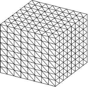
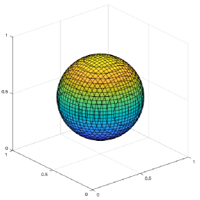
Figure 5: The spherical domain and the tetrahedral mesh of Example 3.

$m$	$h$	1/8	1/16	1/32	1/64	order
$1$	$\|\boldsymbol{u}-\boldsymbol{u}_{h}\|_{L^{2}(\Omega_{0})}$	8.357e-3	2.866e-3	1.042e-3	2.782e-4	1.91
	$\|\boldsymbol{u}-\boldsymbol{u}_{h}\|_{{\mathrm{DG}}}$	1.910e-1	1.143e-1	5.441e-2	2.481e-2	1.13
$2$	$\|\boldsymbol{u}-\boldsymbol{u}_{h}\|_{L^{2}(\Omega_{0})}$	1.946e-3	8.168e-5	7.951e-6	7.897e-7	3.33
	$\|\boldsymbol{u}-\boldsymbol{u}_{h}\|_{{\mathrm{DG}}}$	5.882e-2	8.205e-3	1.797e-3	4.063e-4	2.15
$3$	$\|\boldsymbol{u}-\boldsymbol{u}_{h}\|_{L^{2}(\Omega_{0})}$	8.379e-5	2.828e-6	1.348e-7	7.699e-9	4.13
	$\|\boldsymbol{u}-\boldsymbol{u}_{h}\|_{{\mathrm{DG}}}$	3.793e-3	3.260e-4	3.357e-5	3.602e-6	3.22

Table 3: The numerical errors of Example 3.

5.2 Convergence Studies for Elliptic Interface Problems

This subsection is devoted to verify the theoretical analysis of the interface-unfitted scheme (26). The spaces $V_{h,0}^{m,\circ}$ and $V_{h,1}^{m,\circ}$ are taken as the $C^{0}$ finite element spaces. The penalty parameter $\eta$ is selected as $3m^{2}+10$.

Example 4.

This test is a 2D benchmark problem on $\Omega=(-1,1)^{2}$ that contains a circular interface (see Figure 6),

$$\phi(x,y)=x^{2}+y^{2}-r^{2}=0,\quad\forall(x,y)\in(-1,1)^{2},$$

with radius $r=0.5$. The piecewise coefficient $\alpha$ in (23) and the exact solution are respectively taken to be

$$\alpha=\begin{cases}b,&\phi(x,y)>0,\\ 1,&\phi(x,y)<0,\\ \end{cases}\quad u(x,y)=\begin{cases}-\frac{1}{b}\left(\frac{(x^{2}+y^{2})^{2}}{2}+x^{2}+y^{2}\right),&\phi(x,y)>0,\\ \sin(2\pi x)\sin(\pi y),&\phi(x,y)<0,\\ \end{cases}$$

with $b=10$. We adopt triangular meshes with $h=1/10,\ldots,1/80$ with $1\leq m\leq 3$. Numerical results are collected in Table 4. We can observe that the proposed unfitted method yields $(m+1)$-th and $m$-th convergence rates for the errors $\|u-u_{h}\|_{L^{2}(\Omega)}$ and $|\!|\!|u-u_{h}|\!|\!|_{{\mathrm{DG}}}$, respectively. This is in accordance with the predicted results in Theorem 32.

Figure 6: The interface and the partition of Example 4.

$m$	$h$	1/10	1/20	1/40	1/80	order
$1$	$\|\boldsymbol{u}-\boldsymbol{u}_{h}\|_{L^{2}(\Omega)}$	5.258e-2	1.558e-2	3.081e-3	6.888e-4	2.16
	$\|\boldsymbol{u}-\boldsymbol{u}_{h}\|_{{\mathrm{DG}}}$	9.881e-1	4.747e-1	1.953e-1	9.087e-2	1.10
$2$	$\|\boldsymbol{u}-\boldsymbol{u}_{h}\|_{L^{2}(\Omega)}$	1.055e-3	1.446e-4	1.130e-5	1.208e-6	3.23
	$\|\boldsymbol{u}-\boldsymbol{u}_{h}\|_{{\mathrm{DG}}}$	5.895e-2	1.450e-2	2.788e-3	6.590e-4	2.08
$3$	$\|\boldsymbol{u}-\boldsymbol{u}_{h}\|_{L^{2}(\Omega)}$	7.192e-5	3.885e-6	1.639e-7	9.199e-9	4.15
	$\|\boldsymbol{u}-\boldsymbol{u}_{h}\|_{{\mathrm{DG}}}$	5.176e-3	5.662e-4	5.108e-5	5.908e-6	3.11

Table 4: The numerical errors of Example 4: $b=10$.

Further, we also test the case, by choosing $b=1000$, that the coefficient has a large jump. The numerical results are shown in Table 5. By comparing the errors in Table 4 with Table 5, we demonstrate the robustness of the proposed method for the problem involving a big contrast on the interface.

$m$	$h$	1/10	1/20	1/40	1/80	order
$1$	$\|\boldsymbol{u}-\boldsymbol{u}_{h}\|_{L^{2}(\Omega)}$	5.382e-2	1.819e-2	3.551e-3	7.490e-4	2.24
	$\|\boldsymbol{u}-\boldsymbol{u}_{h}\|_{{\mathrm{DG}}}$	9.818e-1	4.712e-1	2.002e-1	8.368e-2	1.23
$2$	$\|\boldsymbol{u}-\boldsymbol{u}_{h}\|_{L^{2}(\Omega)}$	1.019e-3	1.563e-4	1.132e-5	1.259e-6	3.17
	$\|\boldsymbol{u}-\boldsymbol{u}_{h}\|_{{\mathrm{DG}}}$	5.625e-2	1.547e-2	2.788e-3	6.698e-4	2.06
$3$	$\|\boldsymbol{u}-\boldsymbol{u}_{h}\|_{L^{2}(\Omega)}$	7.331e-5	4.302e-6	2.013e-7	1.048e-8	4.26
	$\|\boldsymbol{u}-\boldsymbol{u}_{h}\|_{{\mathrm{DG}}}$	5.258e-3	6.540e-4	6.369e-5	6.658e-6	3.25

Table 5: The numerical errors of Example 4 with a large jump: $b=1000$.

Example 5.

We consider an elliptic interface problem with a star interface [39] (see Figure 7), where $\Gamma$ is parametrized with the polar coordinate $(r,\theta)$,

$$\phi(r,\theta)=r-\frac{1}{2}-\frac{\sin(5\theta)}{7}.$$

The domain is $\Omega=(-1,1)^{2}$. The coefficient $\alpha$ and the exact solution are selected to be

$$\alpha=\begin{cases}10,&\phi(r,\theta)>0,\\ 1,&\phi(r,\theta)<0,\\ \end{cases}\quad u(r,\theta)=\begin{cases}0.1r^{2}-0.01\ln(2r),&\phi(r,\theta)>0,\\ e^{r^{2}},&\phi(r,\theta)<0,\\ \end{cases}$$

respectively. We display the numerical results in Table 6. Similar as the previous example, the optimal convergence rates for the errors under the $L^{2}$ norm and the energy norm can be still observed.

Figure 7: The interface and the partition of Example 5.

$m$	$h$	1/8	1/16	1/32	1/64	order
$1$	$\|\boldsymbol{u}-\boldsymbol{u}_{h}\|_{L^{2}(\Omega)}$	9.311e-3	2.269e-3	4.456e-4	9.326e-5	2.26
	$\|\boldsymbol{u}-\boldsymbol{u}_{h}\|_{{\mathrm{DG}}}$	1.795e-1	8.026e-2	3.488e-2	1.600e-2	1.12
$2$	$\|\boldsymbol{u}-\boldsymbol{u}_{h}\|_{L^{2}(\Omega)}$	5.070e-4	3.869e-5	3.360e-6	3.493e-7	3.26
	$\|\boldsymbol{u}-\boldsymbol{u}_{h}\|_{{\mathrm{DG}}}$	2.595e-2	2.905e-3	5.623e-4	1.229e-4	2.19
$3$	$\|\boldsymbol{u}-\boldsymbol{u}_{h}\|_{L^{2}(\Omega)}$	1.106e-5	6.759e-7	2.741e-8	1.408e-9	4.28
	$\|\boldsymbol{u}-\boldsymbol{u}_{h}\|_{{\mathrm{DG}}}$	1.361e-3	7.226e-5	6.342e-6	6.693e-7	3.23

Table 6: The numerical errors of Example 5.

Example 6.

In the last example, we consider the elliptic interface problem (23) in three dimensions with the coefficient $\alpha=1$. The domain is the unit cube $\Omega=(0,1)^{3}$ and the interface is a smooth molecular surface of two atoms (see Figure 8), which is given by the level set function [37, 29],

$$\phi(x,y,z)=\left((2.5(x-0.5))^{2}+(4(y-0.5))^{2}+(2.5(z-0.5))^{2}+0.6\right)^{2}-3.5(4(y-0.5))^{2}-0.6.$$

The exact solution takes the form

$$u(x,y,z)=\begin{cases}e^{2(x+y+z)},&\phi(x,y,z)>0,\\ \sin(2\pi x)\sin(2\pi y)\sin(2\pi z),&\phi(x,y,z)<0.\\ \end{cases}$$

The initial mesh $\mathcal{T}_{h}$ is taken as a tetrahedral with $h=1/4$, and we solve the interface problem on a series of successively refined meshes (see Figure 5). The convergence histories with $1\leq m\leq 3$ are reported in Table 7, which show that both errors $\|u-u_{h}\|_{L^{2}(\Omega)}$ and $|\!|\!|u-u_{h}|\!|\!|_{{\mathrm{DG}}}$ decrease to zero at their optimal convergence rates. This observation again validates the theoretical predictions in Theorem 32.

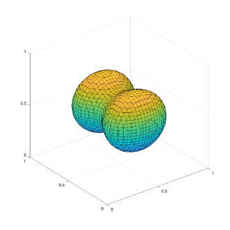
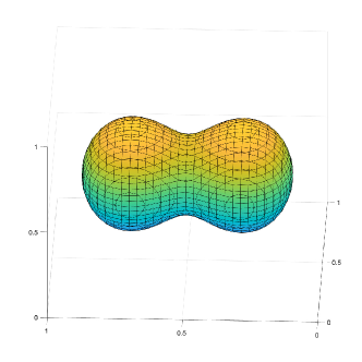
Figure 8: The interface of Example 6.

$m$	$h$	1/4	1/8	1/16	1/32	order
$1$	$\|\boldsymbol{u}-\boldsymbol{u}_{h}\|_{L^{2}(\Omega)}$	1.705e-0	6.021e-1	1.260e-1	2.829e-2	2.15
	$\|\boldsymbol{u}-\boldsymbol{u}_{h}\|_{{\mathrm{DG}}}$	3.656e+1	1.783e+1	7.547e-0	3.675e-2	1.03
$2$	$\|\boldsymbol{u}-\boldsymbol{u}_{h}\|_{L^{2}(\Omega)}$	3.266e-1	2.326e-2	1.823e-3	1.930e-4	3.25
	$\|\boldsymbol{u}-\boldsymbol{u}_{h}\|_{{\mathrm{DG}}}$	4.948e-0	9.037e-1	1.698e-1	3.915e-2	2.12
$3$	$\|\boldsymbol{u}-\boldsymbol{u}_{h}\|_{L^{2}(\Omega)}$	3.609e-1	1.600e-3	7.349e-5	4.111e-6	4.16
	$\|\boldsymbol{u}-\boldsymbol{u}_{h}\|_{{\mathrm{DG}}}$	3.167e-0	7.372e-2	9.519e-3	1.182e-3	3.01

Table 7: The numerical errors of the Example 6.

6 Conclusion

We have developed unfitted finite element methods for the elliptic boundary value problem and the elliptic interface problem. The degrees of freedom of the used approximation spaces are totally located in the elements that are not cut by the domain boundary and interface. The boundary condition and the jump condition are weakly imposed by Nitsche’s method. The stability near the boundary or the interface does not require any stabilization technique or any constraint on the mesh. The optimal convergence orders under the $L^{2}$ norm and the energy norm are proved. In addition, we give upper bounds of the condition numbers for the two final linear systems. A series of numerical examples in two and three dimensions are presented to validate our theoretical results.

References

[1]
R. A. Adams and J. J. F. Fournier, Sobolev Spaces, second ed., Pure
and Applied Mathematics (Amsterdam), vol. 140, Elsevier/Academic Press,
Amsterdam, 2003.
[2]
P. M. A. Areias and T. Belytschko, Letter to the editor: A comment on
the article: “A finite element method for the simulation of strong and
weak discontinuities in solid mechanics” [Comput. Methods Appl.
Mech. Engrg. 193 (2004), no. 33-35, 3523–3540; mr2075053] by A.
Hansbo and P. Hansbo, Comput. Methods Appl. Mech. Engrg. 195
(2006), no. 9-12, 1275–1276.
[3]
I. Babuška and U. Banerjee.
Stable generalized finite element method (SGFEM).
Computer Methods in Applied Mechanics and Engineering,
201(1):91–111, 2011.
[4]
T. Belytschko, R. Gracie, and G. Ventura.
A review of extended/generalized finite element methods for material
modeling.
Modelling and Simulation in Materials Science and Engineering,
17(4):043001, 2009.
[5]
S. P. A. Bordas, E. Burman, M. G. Larson, and M. A. Olshanskii (eds.),
Geometrically unfitted finite element methods and applications,
Lecture Notes in Computational Science and Engineering, vol. 121, Springer,
Cham, 2017, Held January 6–8, 2016.
[6]
S. C. Brenner and L. R. Scott, The Mathematical Theory of Finite Element
Methods, third ed., Texts in Applied Mathematics, vol. 15, Springer, New
York, 2008.
[7]
E. Burman, Ghost penalty, C. R. Math. Acad. Sci. Paris 348
(2010), no. 21-22, 1217–1220.
[8]
E. Burman, M. Cicuttin, G. Delay, and A. Ern, An unfitted hybrid
high-order method with cell agglomeration for elliptic interface problems,
SIAM J. Sci. Comput. 43 (2021), no. 2, A859–A882.
[9]
E. Burman, S. Claus, P. Hansbo, M. G. Larson, and A. Massing, CutFEM:
discretizing geometry and partial differential equations, Internat. J.
Numer. Methods Engrg. 104 (2015), no. 7, 472–501.
[10]
E. Burman and P. Hansbo, Fictitious domain finite element methods using
cut elements: II. A stabilized Nitsche method, Appl. Numer. Math.
62 (2012), no. 4, 328–341.
[11]
, Fictitious domain methods using cut elements: III. A
stabilized Nitsche method for Stokes’ problem, ESAIM Math. Model. Numer.
Anal. 48 (2014), no. 3, 859–874.
[12]
E. Burman, P. Hansbo, M. G. Larson, and A. Massing, A stable cut finite
element method for partial differential equations on surfaces: the
Helmholtz-Beltrami operator, Comput. Methods Appl. Mech. Engrg.
362 (2020), 112803, 21.
[13]
T. Cui, W. Leng, H. Liu, L. Zhang, and W. Zheng, High-order numerical
quadratures in a tetrahedron with an implicitly defined curved interface,
ACM Trans. Math. Softw. (2019), to appear.
[14]
F. de Prenter, C. Lehrenfeld, and A. Massing, A note on the stability
parameter in Nitsche’s method for unfitted boundary value problems,
Comput. Math. Appl. 75 (2018), no. 12, 4322–4336.
[15]
V. Girault and P.-A. Raviart, Finite element methods for
Navier-Stokes equations, Springer Series in Computational Mathematics,
vol. 5, Springer-Verlag, Berlin, 1986, Theory and algorithms.
[16]
C. Gürkan and A. Massing, A stabilized cut discontinuous Galerkin
framework for elliptic boundary value and interface problems, Comput.
Methods Appl. Mech. Engrg. 348 (2019), 466–499.
[17]
, A stabilized cut discontinuous Galerkin framework for elliptic
boundary value and interface problems, Comput. Methods Appl. Mech. Engrg.
348 (2019), 466–499.
[18]
C. Gürkan, S. Sticko, and A. Massing, Stabilized cut discontinuous
Galerkin methods for advection-reaction problems, SIAM J. Sci. Comput.
42 (2020), no. 5, A2620–A2654.
[19]
A. Hansbo and P. Hansbo, An unfitted finite element method, based on
Nitsche’s method, for elliptic interface problems, Comput. Methods Appl.
Mech. Engrg. 191 (2002), no. 47-48, 5537–5552.
[20]
P. Hansbo and M. G. Larson, Discontinuous Galerkin methods for
incompressible and nearly incompressible elasticity by Nitsche’s method,
Comput. Methods Appl. Mech. Engrg. 191 (2002), no. 17-18,
1895–1908.
[21]
P. Hansbo, M. G. Larson, and S. Zahedi, A cut finite element method for a
Stokes interface problem, Appl. Numer. Math. 85 (2014), 90–114.
[22]
Y. Han, H. Chen, X. Wang, and X. Xie.
EXtended HDG methods for second order elliptic interface
problems.
Journal of Scientific Computing, 84(1):22, 2020.
[23]
P. Huang, H. Wu, and Y. Xiao, An unfitted interface penalty finite
element method for elliptic interface problems, Comput. Methods Appl. Mech.
Engrg. 323 (2017), 439–460.
[24]
A. Johansson and M. G. Larson, A high order discontinuous Galerkin
Nitsche method for elliptic problems with fictitious boundary, Numer.
Math. 123 (2013), no. 4, 607–628.
[25]
R. B. Kellogg, Higher order singularities for interface problems, The
mathematical foundations of the finite element method with applications to
partial differential equations (Proc. Sympos., Univ. Maryland,
Baltimore, Md., 1972), 1972, pp. 589–602. MR 0433926
[26]
R. B. Kellogg and J. E. Osborn, A regularity result for the Stokes
problem in a convex polygon, J. Functional Analysis 21 (1976),
no. 4, 397–431.
[27]
C. Lehrenfeld, High order unfitted finite element methods on level set
domains using isoparametric mappings, Comput. Methods Appl. Mech. Engrg.
300 (2016), 716–733.
[28]
C. Lehrenfeld and A. Reusken, Analysis of a high-order unfitted finite
element method for elliptic interface problems, IMA J. Numer. Anal.
38 (2018), no. 3, 1351–1387.
[29]
R. Li and F. Yang, A discontinuous Galerkin method by patch
reconstruction for elliptic interface problem on unfitted mesh, SIAM J. Sci.
Comput. 42 (2020), no. 2, A1428–A1457.
[30]
Z. Li.
The immersed interface method using a finite element formulation.
Applied Numerical Mathematics, 27(3):253–267, 1998.
[31]
T. Lin, Y. Lin, and X. Zhang.
Partially penalized immersed finite element methods for elliptic
interface problems.
SIAM Journal on Numerical Analysis, 53(2):1121–1144, 2015.
[32]
A. Massing, M. G. Larson, A. Logg, and M. E. Rognes, A stabilized
Nitsche fictitious domain method for the Stokes problem, J. Sci. Comput.
61 (2014), no. 3, 604–628.
[33]
B. Rivière, M. F. Wheeler, and V. Girault, Improved energy estimates
for interior penalty, constrained and discontinuous Galerkin methods for
elliptic problems. I, Comput. Geosci. 3 (1999), no. 3-4, 337–360
(2000).
[34]
R. I. Saye, High-order quadrature methods for implicitly defined surfaces
and volumes in hyperrectangles, SIAM J. Sci. Comput. 37 (2015),
no. 2, A993–A1019.
[35]
T. Strouboulis, I. Babuška, and K. Copps.
The design and analysis of the generalized finite element method.
Computer Methods in Applied Mechanics and Engineering,
181(1-3):43–69, 2000.
[36]
P. F. Thomas and B. Ted.
The eXtended/Generalized finite element method: An overview of
the method and its applications.
International Journal for Numerical Methods in Engineering,
84(3):253–304, 2010.
[37]
Z. Wei, C. Li, and S. Zhao, A spatially second order alternating
direction implicit (ADI) method for solving three dimensional parabolic
interface problems, Comput. Math. Appl. 75 (2018), no. 6,
2173–2192.
[38]
H. Wu and Y. Xiao, An unfitted -interface penalty finite element
method for elliptic interface problems, J. Comput. Math. 37 (2019),
no. 3, 316–339.
[39]
Y. C. Zhou and G. W. Wei, On the fictitious-domain and interpolation
formulations of the matched interface and boundary (MIB) method, J.
Comput. Phys. 219 (2006), no. 1, 228–246.