Evaluation of binary classifiers for asymptotically dependent and independent extremes

Abstract

Machine learning classification methods usually assume that all possible classes are sufficiently present within the training set. Due to their inherent rarities, extreme events are always under-represented and classifiers tailored for predicting extremes need to be carefully designed to handle this under-representation. In this paper, we address the question of how to assess and compare classifiers with respect to their capacity to capture extreme occurrences. This is also related to the topic of scoring rules used in forecasting literature. In this context, we propose and study a risk function adapted to extremal classifiers. The inferential properties of our empirical risk estimator are derived under the framework of multivariate regular variation and hidden regular variation. A simulation study compares different classifiers and indicates their performance with respect to our risk function. To conclude, we apply our framework to the analysis of extreme river discharges in the Danube river basin. The application compares different predictive algorithms and test their capacity at forecasting river discharges from other river stations. As a byproduct, we study the special class of linear classifiers, show that the optimization of our risk function leads to a consistent solution and we identify the explanatory variables that contribute the most to extremal behavior.

Keywords: Multivariate Extreme Value Theory; Binary Classification; Multivariate Regular Variation; Hidden Regular Variation; River Discharges

1 Introduction

In binary classification, one typically considers data of the form $(\bm{X},Y)^{\top}$ where $Y\in\{-1,1\}$ represents a binary response to the input $\bm{X}\in[0,\infty)^{d}$. In this paper, we focus on the case that $Y=Y^{(u)}$ represents the occurrence of an extreme event, $Y^{(u)}=1$ indicating that a random quantity $H$ crosses a level $u$, called the threshold, and $Y^{(u)}=-1$ otherwise, that is

$$Y^{(u)}=\begin{cases}+1,&\quad\textup{if }H>u,\\ -1,&\quad\textup{otherwise.}\end{cases}$$ (1)

In the following, for simplicity, we focus on the case that $H$ is a non-negative random variable such that $\operatorname{\mathbb{P}}(H>u)>0$ for all $u>0$ and its upper end point is infinite.

In extreme value analysis, one is interested in the behavior of $Y^{(u)}$ for high levels, that is for $u\to\infty$, and, therefore, also any classifier $g$ needs to be adapted to the threshold $u$. Thus, for every $u>0$, let $g(\cdot;u)$ be a measurable function from $\mathbb{R}^{d}$ to $\{-1,1\}$. In order to evaluate the quality of the classification at a certain level $u$, we consider a loss function $l_{u}$ that assigns a cost to a classifier $g(\cdot;u)$ and a realization $(\bm{x},y^{(u)})$. Here, it is important to note that, by definition of rare events, $\operatorname{\mathbb{P}}(Y^{(u)}=1)$ is very small and $\operatorname{\mathbb{P}}(Y^{(u)}=-1)$ is close to one as $u$ gets large. This imbalance can lead to atypical and/or undesirable comparisons of classifiers. For example, the “always optimistic” classifier that never forecasts an extreme can be defined as $g(\bm{X};u)\equiv-1$, almost surely. To see how to handle this naive classifier, the classical risk function defined as the expectation of the indicator $\mathds{1}\{g(\bm{X};u)\neq Y^{(u)}\}$ can be written as

$$\operatorname{\mathbb{P}}\left(g(\bm{X};u)\neq Y^{(u)}\right)=\operatorname{\mathbb{P}}(H>u,g(\bm{X};u)=-1)+\operatorname{\mathbb{P}}(H\leq u,g(\bm{X};u)=1).$$ (2)

If $g(\bm{X};u)\equiv-1$, then $\operatorname{\mathbb{P}}(g(\bm{X};u)\neq Y^{(u)})=\operatorname{\mathbb{P}}(H>u)$ goes to zero as $u$ gets large. Hence, the classical risk function $\operatorname{\mathbb{E}}(\mathds{1}\{g(\bm{X};u)\neq Y^{(u)}\})$ will systematically favor the always optimistic classifier for extremes. To avoid this undesirable feature, the loss function has to be modified. One natural idea is to re-scale by $\operatorname{\mathbb{P}}(H>u)$ and introduce the loss function $\mathds{1}\{g(\bm{X};u)\neq Y^{(u)}\}/\operatorname{\mathbb{P}}(H>u)$. In this case, the risk, i.e., the expected loss $\operatorname{\mathbb{E}}(\mathds{1}\{g(\bm{X};u)\neq Y^{(u)}\}/\operatorname{\mathbb{P}}(H>u))$, goes towards one as $u$ gets large.

Another trivial but also interesting case is the “crying wolf” forecaster who always issues $g(\bm{X};u)\equiv+1$, see also the forecaster’s dilemma (e.g. Lerch et al.,, 2017). In this case, Equation (2) implies that $\operatorname{\mathbb{P}}\left(g(\bm{X};u)\neq Y^{(u)}\right)=\operatorname{\mathbb{P}}(H\leq u)$ and, consequently, the risk $\operatorname{\mathbb{E}}(\mathds{1}\{g(\bm{X};u)\neq Y^{(u)}\}/\operatorname{\mathbb{P}}(H>u))$ goes towards infinity as $u$ gets large. This limiting cost indicates that the “crying wolf” forecaster is much worse than the overly optimistic one. Both of them are unreasonable in practice and there is no reason to strongly favour one over the other one. For this reason, we propose to use a following weighted loss function

$$l_{u}(g;(\bm{x},y))=\frac{1}{\operatorname{\mathbb{P}}(Y^{(u)}=1\text{ or }g(\bm{X};u)=1)}\mathds{1}\{g(\bm{x};u)\neq y\}$$

and the associated risk

$$R^{(u)}(g)=\operatorname{\mathbb{E}}(l_{u}(g;(\bm{X},Y^{(u)}))=\frac{\operatorname{\mathbb{P}}(g(\bm{X};u)\neq Y^{(u)})}{\operatorname{\mathbb{P}}(Y^{(u)}=1\text{ or }g(\bm{X};u)=1)}.$$ (3)

By construction, the event $\{g(\bm{X};u)\neq Y^{(u)}\}$ implies that $\{Y^{(u)}=1\}$ or $\{g(\bm{X};u)=1\}$ and therefore, necessarily, $R^{(u)}(g)\in[0,1]$. In particular, the naive classifier $g(\bm{X};u)\equiv-1$ possesses unit risk with $R^{(u)}(g)=1$ at each level $u>0$. Similarly, the risk of the “crying wolf” classifier $g(\bm{X};u)\equiv+1$ is then equal to $R^{(u)}(g)=\operatorname{\mathbb{P}}(H\leq u)$ and converges to one as $u\to\infty$.

Hence, the value of one is reached by the two worst cases scenarios in terms of classifiers. This unit value provides a clear benchmark that can be compared to any other classifier satisfying the existence of the limit

$$R(g)=\lim_{u\to\infty}R^{(u)}(g)\in[0,1].$$

We call such classifiers extremal.

In the weather forecast literature (e.g. Schaefer,, 1990), the definition of $R^{(u)}(g)$ can be linked to the critical success index, also called the threat score. The critical success index computes the total number of correct event forecasts (hits) divided by the total number of forecasts plus the number of misses (hits + false alarms + misses). Hence, $1-R^{(u)}(g)$ can be understood as a critical success index for extremes. In the context of rare events forecasts, Stephenson et al., (2008) highlighted some advantages and drawbacks of various risk functions, including the critical success index. In particular, these authors linked forecast scoring rules with two dependence indices used in EVT (see Coles et al.,, 1999)

$$\chi=\lim_{u\rightarrow 1}\operatorname{\mathbb{P}}(U>u\mid V>u)\mbox{ and }\overline{\chi}=\lim_{u\rightarrow 1}\left[ \frac{2\log(\operatorname{\mathbb{P}}(U>u)}{\log(\operatorname{\mathbb{P}}(U>u,V>u))}-1\right],$$

where the two random variables $U$ and $V$ follow the same continuous uniform distribution on $[0,1]$. The choice of uniform marginals can be made whenever the forecast can be assumed to be calibrated, i.e.  observations and forecasts follow the same marginal distributions and can be transformed into uniforms. Concerning the extremal dependence strength between $U$ and $V$, if $\chi>0$, then the variables $U$ and $V$ are said to be asymptotically dependent and $\overline{\chi}=1$. If $\chi=0$, then the variables $U$ and $V$ are said to be asymptotically independent and $\overline{\chi}<1$ captures some second order extremal dependence information. Stephenson et al., (2008) advocated the use of $\overline{\chi}$ and called it the extreme dependency score. Later on, Ferro and Stephenson, (2011) proposed two different scores and studied their properties. But the link with the concept of asymptotic independence was not clear and the convergence results of their estimators were not fully developed. In contrast to $\chi$, one drawback of $\overline{\chi}$ is that its formula is not easy to explain to practitioners. In comparison, $R(g)$ as a type of the critical success index can be interpreted with ease. Hence, it is of interest to extend this definition to the asymptotic independent case.

In the machine learning literature, there is a vast body of work about imbalanced data (see, e.g. Hilario et al.,, 2018). Within this context of imbalanced problems, $R(g)$ can be understood as a function of precision and recall, two metrics well-used to score binary classifiers in learning research (see, e.g. He and Ma,, 2013, and the $F$-score). Still, the review paper by Haixiang et al., (2017) did not mention any imbalanced method based on extreme value theory (see, e.g. Resnick,, 2003). To our knowledge, very few theoretical links have been made to bridge the imbalanced learning and multivariate extreme value theory. One noticeable exception is Jalalzai et al., (2018) who worked on binary classifiers for extremes under the regular variation hypothesis. But they did not focus on $R^{(u)}(g)$. Instead, they studied a different setting where the object of interest was $\operatorname{\mathbb{P}}(g(\bm{X})\neq Y\mid\|\bm{X}\|>u)$ where $\|\bm{X}\|$ represents a norm with $u$ large. Hence, their conditioning event was $\{\|\bm{X}\|>u\}$, while our conditioning depends on $Y$ with the set $\{Y^{(u)}=1\text{ or }g(\bm{X};u)=1\}$, see Equation (3). So, their interest was centered on the classifier performance when the norm of the explanatory vector $\bm{X}$ was large. Our focus is on large values of $H$ in the production of extreme events of the type $Y^{(u)}=1$ when $H>u$, see Equation (1). Jalalzai et al., (2018) provided various theoretical results based on the main assumption that the conditional distribution of $\bm{X}$ given $Y=\pm 1$ was regularly varying with an angular measure that depends on $Y=\pm 1$.

In this study, one part of our results is based on the concept of hidden regular variation (see, e.g. Ledford and Tawn,, 1996; Heffernan and Resnick,, 2005; Ferro,, 2007). In particular, we take advantage of the model of Ramos and Ledford, (2009) to derive the asymptotic properties of our estimators.

Our paper is organized as follows. In Section 2, we propose and study a risk function that can handle both the asymptotic dependent and independent cases. Estimators are also constructed and their asymptotic properties derived. Section 3 focuses on a simulation example that highlights the difficulty to compare common classifiers in the case of asymptotic independence. In Section 4, we revisit the well studied example of the Danube river application and see how the choice of the metric can change the ranking of classifiers. Note that, besides the proofs of all propositions, the appendix addresses the questions of how to optimize the linear classifier for extremes and how to choose the relevant features, see Section B.

2 Risk, upper tail equivalence and extremal dependence

The following lemma provides a flexible blueprint to link risk functions with probabilities based on general sets. We will apply it under different setups linked to extreme events.

Lemma 1

Let $A_{\varepsilon}$ be a sequence of measurable sets of increasing sizes with decreasing $\varepsilon\in[0,1]$, in particular $A_{1}\subseteq A_{\varepsilon}\subseteq A_{0}$. Let $B_{\varepsilon}$ be the same type of set sequence such that $\operatorname{\mathbb{P}}(A_{1}\cap B_{1})>0$. The following ratio $R(A_{\varepsilon},B_{\varepsilon})$ can be written as

$$R(A_{\varepsilon},B_{\varepsilon})\coloneqq\frac{\operatorname{\mathbb{P}}(A_{1}\triangle B_{1}\mid A_{\varepsilon}\cap B_{\varepsilon})}{\operatorname{\mathbb{P}}(A_{1}\cup B_{1}\mid A_{\varepsilon}\cap B_{\varepsilon})}=1-\left[\frac{1}{\operatorname{\mathbb{P}}(B_{1}|A_{1}\cap B_{\varepsilon})}+\frac{1}{\operatorname{\mathbb{P}}(A_{1}\mid A_{\varepsilon}\cap B_{1})}-1\right]^{-1},$$ (4)

where $A_{1}\triangle B_{1}$ denotes the symmetric difference. In addition, we have the three following properties for $R$:

1. $R(A_{\varepsilon},B_{\varepsilon})$ is non-increasing in $\varepsilon$ with $R(A_{1},B_{1})=0$.

2. Let $A^{\prime}_{\varepsilon}$ be another sequence of measurable sets of increasing sizes with decreasing $\varepsilon$.
   If $A_{1}=A^{\prime}_{1}$ and $A_{\varepsilon}\subseteq A^{\prime}_{\varepsilon}$ for some $\varepsilon\in[0,1)$ then

   $$R(A_{\varepsilon},B_{\varepsilon})\leq R(A^{\prime}_{\varepsilon},B_{\varepsilon}).$$

3. If for any $\varepsilon\in[0,1]$ and $\varepsilon^{\prime}\in[0,1]$, there exist some positive constants $a$ and $b$ and some positive function $c_{\varepsilon,\varepsilon^{\prime}}$ such that

   $$\operatorname{\mathbb{P}}(A_{\varepsilon}\cap B_{\varepsilon^{\prime}})=c_{\varepsilon,\varepsilon^{\prime}}\operatorname{\mathbb{P}}^{a}(A_{\varepsilon})\operatorname{\mathbb{P}}^{b}(B_{\varepsilon^{\prime}}),$$ (5)

   then

   $$R(A_{\varepsilon},B_{\varepsilon})=1-\left[\frac{c_{\varepsilon,1}}{c_{1,1}}(\operatorname{\mathbb{P}}(A_{1}\mid A_{\varepsilon}))^{-a}+\frac{c_{1,\varepsilon}}{c_{1,1}}(\operatorname{\mathbb{P}}(B_{1}\mid B_{\varepsilon}))^{-b}-1\right]^{-1}.$$ (6)

We deduce from Equation (4) that $R(A_{\varepsilon},B_{\varepsilon})=0$ if and only if $\operatorname{\mathbb{P}}(B_{1}\mid A_{1}\cap B_{\varepsilon})=\operatorname{\mathbb{P}}(A_{1}\mid A_{\varepsilon}\cap B_{1})=1$. The second property of this lemma indicates that, for a given $\varepsilon$, the risk function becomes smaller if the set $A_{\varepsilon}$ is as small as possible.

Equation (5) can be viewed as a mixing condition that leads to a simple expression of $R(A_{\varepsilon},B_{\varepsilon^{\prime}})$ based on disjoint events.

We want to use the ratio (4) in order to generalize the risk $R^{(u)}(g)$ defined in (3). In the latter definition, adapted to extremes, the set $\{H>u\}$ was considered and one could set $B_{1}=\{H>u\}$, for instance, and consequently, $B_{\varepsilon}=\{H>\varepsilon u\}$ would be a natural sequence if $H$ is regularly varying. The choice of $A_{\varepsilon}$ is open and it can play an important role. In the next paragraphs, we set $\varepsilon=0$ and discuss the choice of $A_{1}$ and $A_{0}$. In Section 2.1, we will work with $\varepsilon>0$. In that case, we will call the corresponding risk the conditional risk.

In the rest of this paper, we restrict our attention on a particular form of classifiers

$$g(\bm{X};u)=\begin{cases}+1,&\quad\textup{if }\overline{g}(\bm{X})>u,\\ -1,&\quad\textup{otherwise,}\end{cases}$$ (7)

for some function $\overline{g}:\mathbb{R}^{d}\to(0,\infty)$. The function $\overline{g}(.)$ does not have to be a norm. It can be understood as any projection/summary of the explanatory variables $\bm{X}$ onto the positive real line (see, e.g. Aghbalou et al.,, 2021, for projection techniques for extremes). This corresponds to the set $A_{1}=\{\overline{g}(\bm{X})>u\}$ in Lemma 1. A special case of this lemma is to set $\varepsilon=0$ and when $A_{0}$ and $B_{0}$ are equal to the full set, i.e. $\operatorname{\mathbb{P}}(A_{0})=\operatorname{\mathbb{P}}(B_{0})=1$, and $A_{1}=\{\overline{g}(\bm{X})>u\}$ and $B_{1}=\{H>u\}$. In this case, Equation (4) tells us that $R^{(u)}(\overline{g})$ defined by (3) satisfies

$$R^{(u)}(\overline{g})=1-\left[\frac{1}{\operatorname{\mathbb{P}}(H>u\mid\overline{g}(\bm{X})>u)}+\frac{1}{\operatorname{\mathbb{P}}(\overline{g}(\bm{X})>u\mid H>u)}-1\right]^{-1}.$$

This leads to the following expression of $R^{(u)}(\overline{g})$

$$R^{(u)}(\overline{g}) {}={}1-\frac{\operatorname{\mathbb{P}}(\overline{g}(\bm{X})>u\mid H>u)}{1-\operatorname{\mathbb{P}}(\overline{g}(\bm{X})>u\mid H>u)+\operatorname{\mathbb{P}}(\overline{g}(\bm{X})>u)/\operatorname{\mathbb{P}}(H>u)}.$$ (8)

Within the class defined by Equation (7), the effect of the marginal distributions of $H$ and $\overline{g}(\bm{X})$ on $R(\overline{g})$ can be explained. When $\overline{g}(\bm{X})$ has a lighter tail than $H$, i.e. $\operatorname{\mathbb{P}}(\overline{g}(\bm{X})>u)/\operatorname{\mathbb{P}}(H>u)\to 0$, then we also have $\operatorname{\mathbb{P}}(\overline{g}(\bm{X})>u\mid H>u)\to 0$, and consequently

$$R^{(u)}(\overline{g})\rightarrow 1,\mbox{ as ${u\to\infty}$.}$$

In the case where $\overline{g}(\bm{X})$ possesses a heavier tail than $H$, i.e. $\operatorname{\mathbb{P}}(\overline{g}(\bm{X})>u)/\operatorname{\mathbb{P}}(H>u)\to\infty$, we can also show that

$$R^{(u)}(\overline{g})\rightarrow 1,\mbox{ as ${u\to\infty}$.}$$

This indicates that, whenever $\overline{g}(\bm{X})$ and $H$ are not tail equivalent, the classifier $\overline{g}(\bm{X})$ cannot outperform naive classifiers with respect to $R^{(u)}(\overline{g})$ for large $u$. Hence, the marginal behavior of $\overline{g}(\bm{X})$ has a direct impact of its predicting capacity in terms of $R(\overline{g})$. This is a widely known fact in forecast verification. In particular, a paradigm promoted by Gneiting and his co-authors (see, e.g. Gneiting et al.,, 2007) is to work only with calibrated forecasts. In our case, calibration means that $\overline{g}(\bm{X})$ and $H$ have the same distributions, and consequently $\operatorname{\mathbb{P}}(\overline{g}(\bm{X})>u)/\operatorname{\mathbb{P}}(H>u)=1$ for all $u$. In practice, it may be difficult to ensure that this constraint holds for extremes (see, e.g. Lerch et al.,, 2017; Taillardat et al.,, 2019). To illustrate this, suppose that $\operatorname{\mathbb{P}}(X>u)=u^{-1}$ for all $u\geq 1,$ and the variable $H$, independently of the value of $X$, is either equal to $\delta X$ or $(2-\delta)X$ with probability $.5$ and the constant $\delta\in(0,1)$. Then, we have

$$\operatorname{\mathbb{P}}(H>u)=\frac{1}{2}\operatorname{\mathbb{P}}\left(\delta X>u\right)+\frac{1}{2}\operatorname{\mathbb{P}}\left((2-\delta)X>u\right)=\begin{cases}\operatorname{\mathbb{P}}(X>u),&\quad\textup{if }u\geq 2-\delta,\\ \frac{1}{2}\left(1+\frac{\delta}{u}\right),&\quad\textup{if }\delta<u\leq 2-\delta,\\ 1,&\quad\textup{if }\delta\geq u.\\ \end{cases}$$

Hence, $X$ and $H$ are more than tail equivalent, they have identical tail behavior for large $u$. Concerning classifiers, linear ones of the type $\overline{g}_{a}(X)=aX$ with $a>0$ belong to the class defined by (7). They are tail equivalent to $H$, and $R(\overline{g}_{a})<1$. Although $X$ and $H$ have identical tail behaviors, the choice of $a=1$ is not optimal with respect to $R(\overline{g}_{a})$. In particular, one can show that

$$R(\overline{g}_{2-\delta})={\frac{1-\delta}{2-\delta}}<R(\overline{g}_{1})={\frac{2-2\delta}{3-\delta}}.$$

This is not surprising. By construction, the largest values of $H$ are more likely to be produced by $(2-\delta)X$ than $X$, especially if $\delta$ is small. In this context, the following lemma explains that the risk function $R(\overline{g})$ both depend on the upper tail dependence between $\overline{g}(\bm{X})$ and $H$ and their marginal behaviors.

Lemma 2

Assume that the two limits

$$c(\overline{g})\coloneqq\lim_{u\to\infty}\frac{\operatorname{\mathbb{P}}(\overline{g}(\bm{X})>u)}{\operatorname{\mathbb{P}}(H>u)}\in(0,\infty)$$

and

$$\chi^{*}(\overline{g})\coloneqq\lim_{u\to\infty}\operatorname{\mathbb{P}}(\overline{g}(\bm{X})>u\mid H>u)\in[0,1]$$

exist. Then, $\chi^{*}(\overline{g})\leq c(\overline{g})$ and the limiting risk based on (3) has the expression

$$R(\overline{g})=1-\frac{\chi^{*}(\overline{g})}{1+c(\overline{g})-\chi^{*}(\overline{g})}.$$ (9)

In particular,

$$R(\overline{g})=0\mbox{ if and only if }c(\overline{g})=\chi^{*}(\overline{g})=1.$$

This lemma indicates that $c(\overline{g})=1$, i.e. $\bar{g}(\bm{X})$ and $H$ are “asymptotically calibrated”, is a necessary condition to have $R(\bar{g})=0$. In the above example with $\delta=0$, we have $c(\overline{g}_{2})=1$ and $R(\overline{g}_{2})=1/2\neq 0$. This means that $\chi^{*}(\overline{g}_{2})<1$. Note that $c(\overline{g})=1$ implies that the constant $\chi^{*}(\overline{g})$ simply corresponds to the aforementioned tail dependence coefficient $\chi$, denoted $\chi(\overline{g})$, and so, the case $c(\overline{g})=1$ simplifies the expression of the risk

$$R(\overline{g})=1-\frac{\chi(\overline{g})}{2-\chi(\overline{g})}.$$

This equality tells us that any asymptotically calibrated classifier with $\chi(\overline{g})=0$ always produces a risk function $R(\overline{g})=1$. Consequently, any asymptotically independent classifier is as uninformative as the two naive classifiers. A reasonable strategy will be to dismiss all asymptotically independent classifiers and find/construct new asymptotically dependent classifiers with positive $\chi(\overline{g})$. But, finding asymptotically dependent classifiers can be complex in practice, and in addition, in some not so exotic setups, this is not always possible. To see this, we consider the simple non-linear regression model in the following lemma.

Lemma 3

Assume that the variable $H$ in (1) is generated by the non-linear regression model

$$H\overset{\mathrm{d}}{=}f(\bm{X})+N,$$

where $\overset{\mathrm{d}}{=}$ represents the equality in distribution, $N$ corresponds to a random noise and $\bm{X}$ corresponds to the explanatory variables, independent of $N$. If $\operatorname{\mathbb{P}}(f(\bm{X})>u)=o\left(\operatorname{\mathbb{P}}(N>u)\right),$ then for any classifier of the type defined by (7), we always have

$$R(\overline{g})=1.$$

Hence, no classifier can outperform naive classifiers for this regression model.

Note that even if the forecaster knows exactly the function $f(.)$ and has drawn from the explanatory $\bm{X}$, the “ideal” classifier ${\overline{g}(\bm{x})=}f(\bm{x})$ will perform badly, i.e. $R(f)=1$. In addition, the classical trick of using ranks to avoid the problem of marginals discrepancy cannot be applied here. For example, suppose that $H$ is unit Fréchet distributed, then transforming the marginals of $\bm{X}$ into unit Fréchet random variables, say into $\bm{\tilde{}}{\bm{X}}$, does not remove the issue as the unobserved noise $N$ has still have heavier tails than $\tilde{f}(\bm{\tilde{X}})=f(\bm{X})$ for some function $\tilde{f}(.)$. So, a finer risk measure is needed that is able to distinguish different classifiers in case of asymptotic independence.

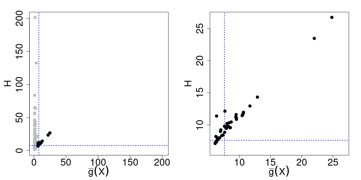
Figure 1: Simulated example for Lemma 3, for more details see equations (13) and (14).

2.1 Conditional risk and hidden regular variation

The choice of the conditioning set in Lemma 1 brings new possibilities to construct finer risk measures for extremes than $R^{(u)}$. To do so, we opted for the sets: $A_{1}=\{\overline{g}(\bm{X})>u\}$ and $B_{1}=\{H>u\}$, (when $\varepsilon=1$) and $A_{0}=\{\overline{g}(\bm{X})>0\}$ and $B_{0}=\{H>0\}$ (when $\varepsilon=0$). But, changing the size of the sets $A_{\varepsilon}$ and $B_{\varepsilon}$ to make them closer to $A_{1}$ and $B_{1}$, will increase the conditional probabilities $\operatorname{\mathbb{P}}(B_{1}\mid A_{1}\cap B_{\varepsilon})$ and $\operatorname{\mathbb{P}}(A_{1}\mid A_{\varepsilon}\cap B_{1})$. A simple choice when $\varepsilon\neq 0$ or $\varepsilon\neq 1$ is to set $A_{\varepsilon}=\{\overline{g}(\bm{X})>\varepsilon u\}$ and $B_{\varepsilon}=\{H>\varepsilon u\}$ with $\varepsilon>0$. This modeling strategy is at the core of hidden regular variation and asymptotic independent models. More precisely, we first need to fix marginal features. We assume that both $\overline{g}(\bm{X})$ and $H$ possess regularly varying tails with indices $\alpha_{g}>0$ and $\alpha_{H}>0$, respectively. This means that for any $\varepsilon\in(0,1)$,

$$\lim_{u\to\infty}\operatorname{\mathbb{P}}(\overline{g}(\bm{X})>u\mid\overline{g}(\bm{X})>\varepsilon u)=\varepsilon^{\alpha_{g}}\mbox{ and }\lim_{u\to\infty}\operatorname{\mathbb{P}}(H>u\mid H>\varepsilon u)=\varepsilon^{\alpha_{H}}.$$

These limits have to be understood with respect to Equation (6), i.e. the terms $\operatorname{\mathbb{P}}(A_{1}\mid A_{\varepsilon})$ and $\operatorname{\mathbb{P}}(B_{1}\mid B_{\varepsilon})$. To apply (6), the mixing condition (5) needs to be satisfied. To do so, we opt for an extended version of the framework of Ramos and Ledford, (2009), i.e.

$$\operatorname{\mathbb{P}}[\overline{g}(\bm{X})>u,H>v]=L(u,v)(u^{-\alpha_{g}}v^{-\alpha_{H}})^{1/2\eta},$$ (10)

where $\eta\in(0,1]$ indicates the rate of decay of the joint survival function and $L(\cdot,\cdot)$ is bivariate slowly varying function, i.e. there exists a limit function $\ell:(0,\infty)\times(0,\infty)\to(0,\infty)$ defined as

$$\ell(s,t)=\lim_{u\to\infty}\frac{L(us,ut)}{L(u,u)},\qquad s,t>0$$

and satisfying $\ell(cs,ct)=\ell(s,t)$ for all $c,s,t>0$. The parameter $\eta$ measures the dependence strength. The case $\eta=1$ corresponds to the asymptotic dependence while $\eta<1$ to the asymptotic independence case. In particular, if $\eta=.5$, then independence appears in the extremes. If $.5<\eta<1$ ($0<\eta<.5)$ the extremal dependence is said to be positively (negatively) associated.

Now, noticing that (10) corresponds to the mixing condition (5), we can apply Lemma 1, see Appendix A for a proof.

Proposition 4

Under the Ramos and Ledford model defined by (10), the following risk function

$$R_{\varepsilon}(g)\coloneqq\lim_{u\to\infty}\frac{\operatorname{\mathbb{P}}(g(\bm{X};u)\neq Y^{(u)}\mid Y^{(\varepsilon u)}=g(\bm{X};\varepsilon u)=1)}{\operatorname{\mathbb{P}}(Y^{(u)}=1\text{ or }g(\bm{X};u)=1\mid Y^{(\varepsilon u)}=g(\bm{X};\varepsilon u)=1)},$$ (11)

which will henceforth also be called conditional risk, can be expressed as

$$R_{\varepsilon}(g)=1-\frac{1}{{\ell(\varepsilon,1)}\varepsilon^{-\alpha_{g}/2\eta}+{\ell(1,\varepsilon)}\varepsilon^{-\alpha_{H}/2\eta}-1},\mbox{ for any $\varepsilon\in[0,1)$.}$$

Note that $\eta\in(0,1]$ takes a similar role as $\chi$ in the case of the unconditional risk $R$.

For fixed $\varepsilon\in[0,1)$, the risk function $R_{\varepsilon}(g)$ decreases with increasing $\eta$. So, given all parameters are fixed but $\eta$, the forecaster should aim at maximizing $\eta$. In practice, two forecasters, say $g_{1}$ and $g_{2}$, may produce different $\ell(.,.)$ and $\alpha_{g}$. Consequently, the minimization of $R_{\varepsilon}(g)$ can also depend, besides $\eta$, on other parameters.

2.2 Risk function inference

Concerning the estimation of $R_{\varepsilon}(g)$ defined by (11), the empirical estimator can be easily computed from the sample $(\bm{X}_{i},H_{i})_{i=1,\dots,n}$. The following proposition describes the asymptotic property of such an estimator.

Proposition 5

Assume that the risk function $R_{\varepsilon}(g)$ defined by (11) exists for a sequence of $u_{n}\to\infty$ such that $np_{g,\varepsilon}(u_{n})\to\infty$ with

$$p_{g,\varepsilon}(u_{n})\coloneqq\operatorname{\mathbb{P}}(\max\{g(\bm{X};u_{n}),Y^{(u_{n})}\}=1,H>\varepsilon u_{n},g(\bm{X};\varepsilon u_{n})=1).$$

If

$$\lim_{n\to\infty}\sqrt{np_{g,\varepsilon}(u_{n})}\left(\frac{\operatorname{\mathbb{P}}(g(\bm{X};u_{n})\neq Y^{(u_{n})},H>\varepsilon u_{n},g(\bm{X};\varepsilon u_{n})=1)}{p_{g,\varepsilon}(u_{n})}-R_{\varepsilon}(g)\right)=0,$$

then the empirical estimator based on a sample $(g(\bm{X}_{i};u),\{H_{i}>u\})_{i=1,\dots,n}$ and defined by

$$\widehat{R}_{n,\varepsilon}(g)=\frac{\sum_{i=1}^{n}\mathds{1}\{g(\bm{X}_{i};u_{n})\neq Y^{(u_{n})}_{i},H_{i}>\varepsilon u_{n},g(\bm{X}_{i};\varepsilon u_{n})=1\}}{\sum_{i=1}^{n}\mathds{1}\{\max\{g(\bm{X}_{i};u_{n}),Y^{(u_{n})}_{i}\}=1,H_{i}>\varepsilon u_{n},g(\bm{X}_{i};\varepsilon u_{n})=1\}}.$$ (12)

converges in distribution in the following way

$$\sqrt{np_{g,\varepsilon}(u_{n})}\left(\widehat{R}_{n,\varepsilon}(g)-R_{\varepsilon}(g)\right)\stackrel{{\scriptstyle n\to\infty}}{{\longrightarrow}}\mathcal{N}\left(0,R_{\varepsilon}(g)(1-R_{\varepsilon}(g))\right).$$

3 Simulations

3.1 A simple linear setup

Our main simulated example is based on a simple linear regression model but with the feature that the explanatory variables $\bm{X}$ do not have the same tail behavior and the noise is regularly varying, see Lemma 3. More precisely, the multivariate vector $\bm{X}$ is defined as follows

$$\left\{\begin{aligned} X_{1}&\sim\mathrm{Pareto}(3)\\ X_{2}&\sim\mathrm{Pareto}(2)\\ X_{3}&\sim\mathrm{Exp}(1)\\ X_{4}&\sim\mathrm{Exp}(2)\end{aligned}\right.,$$ (13)

where all $X_{i}$ are independent with $X_{1}$ and $X_{2}$ Pareto distributed with respective tail index $2$ and $3$, and $X_{3}$ and $X_{4}$ exponentially distributed with respective scale parameters $1$ and $2$. The variable of interest $H$ is simply a linear transform of $X_{1}$ tainted by an additive noise

$$H\overset{\mathrm{d}}{=}X_{1}+N,$$ (14)

where $N\sim\mathrm{Pareto}(2)$ represents an independent noise with heavier tail than $X_{1}$. So, given a sample $(\{X_{j,i}\}_{1\leq j\leq 4},H_{i})_{i=1,\dots,n}$ with $n=10000$, our goal is to compare different classifiers in terms of predicting extreme occurrences, here defined as $\{H>u\}$ with $u$ equal to the $97$th percentile of $H$. In this simulation setup, it is clear from (14) that all variables but $X_{1}$ are useless to explain $H$. In addition, Lemma 3 tells us that the relevant information contained in the variable $X_{1}$ is hidden by the heavier noise $N$, i.e. we are in the case of asymptotic independence.

An example of such simulation is given in Figure 1. The left panel displays a scatter plot between $H$ (left axis) and $\overline{g}(\bm{X})=X_{1}$ (right axis). As expected, no sign of asymptotic dependence can be found in the upper corner. In the right panel, we remove the mass along the axis (gray points) by conditioning on the joint event $A_{\varepsilon}\cap B_{\varepsilon}=\{\overline{g}(\bm{X})>\varepsilon u\}\cap\{H>\varepsilon u\}$ with $\varepsilon=.7$, see all dark points. The right panel zooms on these black points and highlights a clear dependence between $H$ and $X_{1}$ that was hidden by the heavier noise $N$ in $H=X_{1}+N$.

In practice, we do not know the optimal choice for $\overline{g}(.)$ and we need to introduce different classifiers and compare them.

3.2 Classifiers descriptions

Table 1 below provides the list of classifiers that we compare with our metric (12). This list contains some of the most standard classifiers found in the literature (see, e.g. Hastie et al.,, 2009): logistic regression (Logistic), decision tree (Tree), random forest (RF) and support vector machine (SVM).

Table 1: Summary and key features of the different classifiers studied. See for example Hastie et al., (2009) for a comprehensive review of the last four classification methods.

Method	Main features
Linear classifier	Simple binary classifier, parameters estimation based on the minimization of the risk function over the set of contributing variables, theoretical value of $R(g_{\theta})$ inferred from spectral decomposition.
Logistic regression	Parametric linear model with a lasso penalty, coefficients of less contributing variables are set to zero.
Decision trees	Easy to interpret, gives relative importance of each variables, learns simple decision rules inferred from the input.
Random forests	Builds multiple decision trees combined by majority vote, better predictive power than decision trees.
Support vector machines	Finds the best hyperplane to separate two overlapping classes, generally performs better than the other classifiers.

Except for the linear classifier, we apply them with their built-in cost function that is not necessarily fine-tuned to forecast extremes. This is not an issue because our main goal is to compare existing forecasters, and not to create new ones (see, e.g. Jalalzai et al.,, 2018, for such developments). Still, to fix a baseline in terms of performance, the linear classifier defined as

$$g_{\bm{\theta}}(\bm{X};u)=\begin{cases}+1,&\quad\bm{\theta}^{\top}\bm{X}>u,\\ -1,&\quad\bm{\theta}^{\top}\bm{X}\leq u,\end{cases}\qquad\bm{\theta}\in[0,\infty)^{d}.$$

should be optimal for the linear model (14), especially if the regression parameters are estimated by minimizing our cost function (11). In such a context, we expect the linear classifier to be the best. In Appendix B, Proposition 6 provides the condition of the consistency of the estimator $\hat{\bm{\theta}}_{n,u_{n}}$ based on minimizing $\hat{R}_{n}(g_{\bm{\theta}}(\cdot;u_{n}))$ under a regularly varying framework.

The binary outputs from the decision tree classifier are explained in Figure 2. The light blue and light green regions represent the set of points that are well predicted by the classifier. On the contrary, wrongly classified points belong to the light yellow and light red regions: either an extreme is predicted when it is not (light red region), or an extreme event is missed (light yellow region). The difference between the left and right panels corresponds to the training set based on either $\{H>u\}$ or on $\{H>\varepsilon u\}$, i.e. mass removed in the latter case, see also (12).

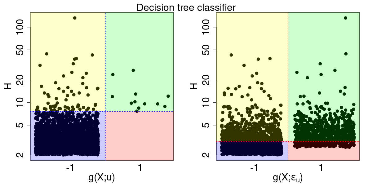
Figure 2: Example of predicted binary output for the decision tree classifier versus the true values of $H$ (on a logarithmic scale). The classifier has been trained twice as explained below. On the left-hand side the classifier is trained with the subset $\{H>u\}$ and the horizontal blue dashed line represents the threshold value $u$. On the right-hand side the classifier is trained with the subset $\{H>\varepsilon u\}$ and the horizontal red dashed line represents the threshold value $\varepsilon u=0.4\times u$. The results shown are the predicted values made upon the testing set whose sample size is equal to $3000$ ($30\%$ of the data).

3.3 Implementation and results

We split our simulated data set in two: $70\%$ for a training part, over which we train our different classifiers to get good predictive power; $30\%$ for a testing part, which we use to estimate the risks $R_{0}(g)$ and $R_{\varepsilon}(g)$. Note that each algorithm has the same inputs, in particular the same binary sequence describing the events $\{H>u\}$ with $u$ set to be equal to the $97$th percentile of $H$. This cross-validation procedure has been repeated $50$ times. The sample used to compute our risk function is based on the bivariate binary vector $(g(\{X_{j,i}\}_{1\leq j\leq 4};u),\{H_{i}>u\})_{i=1,\dots,n}$ where the output of the classifier $g$ is binary. In addition, the binary outputs of the classifier $g$ are obtained under the threshold $u$ and the threshold $\varepsilon u$, so the training part has to be performed twice (once for each threshold). Then, the empirical risk estimator defined by (12) can be computed. Figure 3 shows the sensitivity of the classifier ranking with respect to the value of $\varepsilon$.

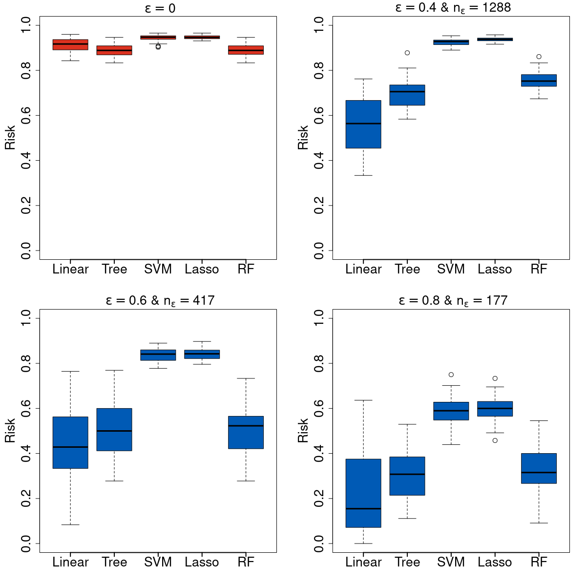
Figure 3: Estimation of $R_{\varepsilon}(g)$ for different classifiers (cross-validation with $50$ repetitions). In red (top-left) are the estimates when $\varepsilon=0$ and in blue for different values of $\varepsilon>0$ ($\varepsilon\in\{0.4,0.6,0.8\}$). At the top of each plot, the value of $\varepsilon$ and the number of points such that $H>\varepsilon u$ from the testing set are given.

As expected from Lemma 3, the top-left panel, that corresponds to the case $\varepsilon=0$, clearly indicates that our five classifiers cannot outperform naive classifiers as all classifiers have a risk near to one, the worst possible value. To start discriminating classifiers, we need to remove the masses along the axes by setting a value for $\varepsilon$. As we increase $\varepsilon$, the size of sets needed to compute (12) becomes smaller, see the values of $n_{\varepsilon}$ in the legend of each panel. Hence, the blue box plots becomes wider as $\varepsilon$ increases: a classical bias-variance trade-off. As we know from (14) that the true generative process is linear, $\varepsilon=0.4$ appears as a reasonable value to balance the bias-variance trade-off. More importantly, the overall ranking is not sensitive to the values of $\varepsilon>0$. In all cases, our linear classifier tailored to handle linear asymptotic independence cases outperforms all the other classifiers. Among the other classifiers, decision tree appears to be the best, but it is still far from the optimal linear solution. Other simulations concerning the regular variation case are available upon request.

4 Danube river discharges

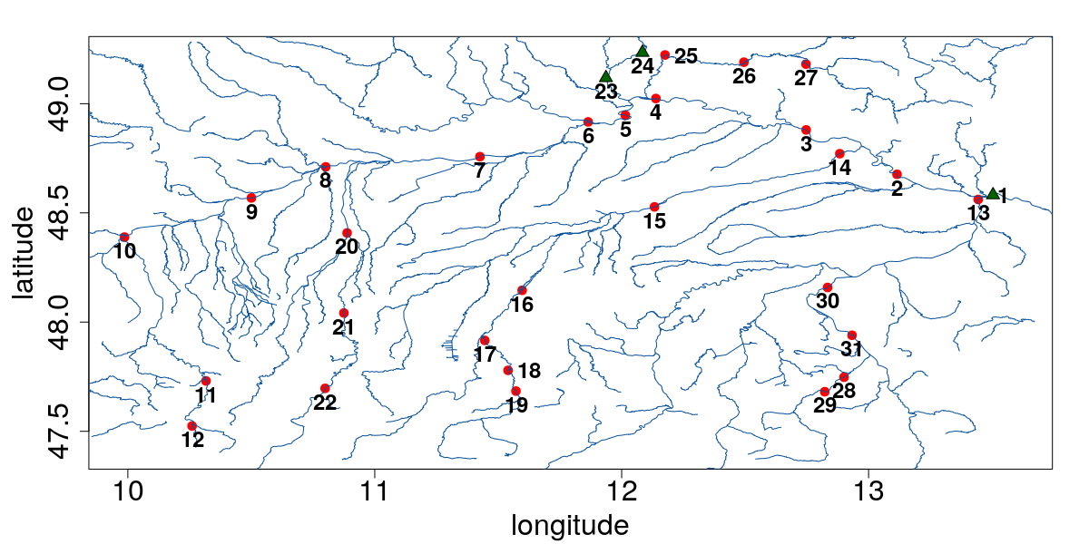
Figure 4: River map of the upper Danube basin, showing sites of the 31 gauging stations along the Danube and its tributaries. Water flows toward gauging station $1$. The stations represented by a green triangle shaped dot are the three stations of interest as described in Section 4.

We now apply our assessment approach to summer daily river discharges (measured in $m^{3}/s$) at $31$ stations spread over the upper Danube basin, see Figure 4, and recorded over the time period 1960-2010 in June, July and August. These observations have been studied by the EVT community (see, e.g. Asadi et al.,, 2015; Mhalla et al.,, 2020; Gnecco et al.,, 2021). This dataset was made available by the Bavarian Environmental Agency (http://www.gkd.bayern.de). To remove temporal clustering in extreme river discharges, Mhalla et al., (2020) in their Section 5 implemented a declustering step. Each station then contains $n=428$ observations that we will consider temporally independent. In order to reduce the large discrepancy in terms of discharges magnitude among stations, we force the starting value of all $31$ time series to equal zero by subtracting to each station its minimum. Then, we re-normalize each time series by its range (i.e. the difference between the maximum and the minimum of each time series).

These post processing treatments are useful to display and interpret the data at hand and do not impact the classifiers performance.

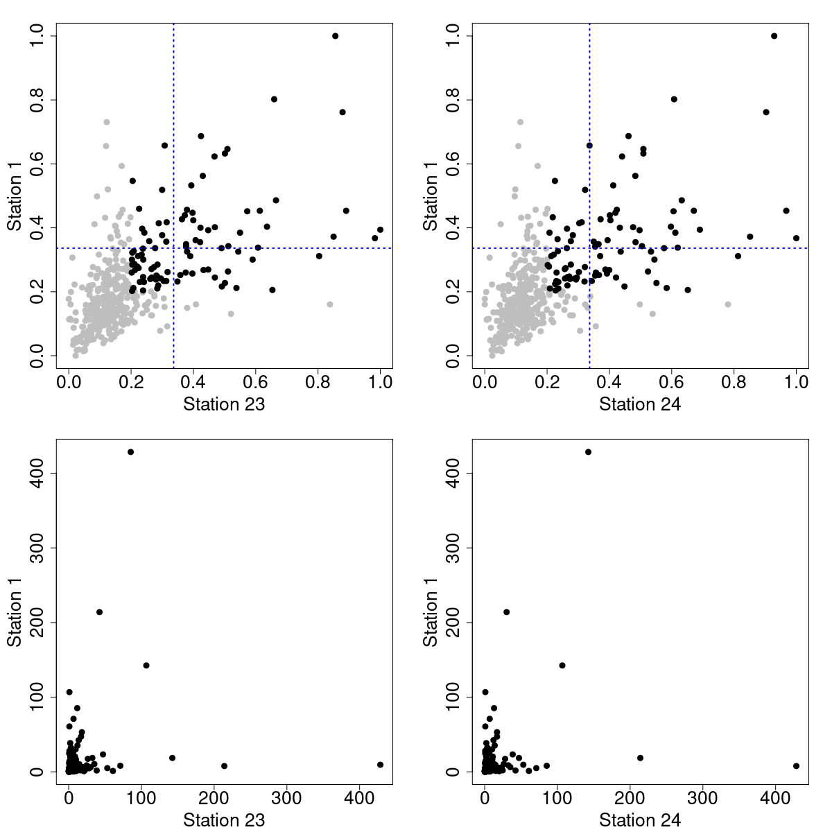
Figure 5: Summer daily measurements of river discharges from station 1 (y-axis) against station $23$ (left x-axis) and station $24$ (right x-axis) of Figure 4. The blue dotted lines are the threshold value u (the $85$th percentile of station $1$). The black dots on the graphs in the top row are the values such that $\min(X_{j},X_{1})>\varepsilon u$ where $\varepsilon u=0.6u$. The graphs in the bottom row corresponds to the same data plots but on unit Fréchet scale highlighting potential asymptotic independence in the data.

Although all $31$ station recordings are available, we can artificially remove one station and try to predict its values from a given subset of other weather stations. In this section, we remove station $1$ (downstream) and try to predict its values from only stations $23$ and $24$, which are indirect tributaries to the main river flow. So, this setup is complex for two reasons. First, station $1$, as a downstream point that accumulates all discharges, has a much heavier tail than the two tributaries. Second, it is difficult to determine if we are in the asymptotic dependent or independent case, see Figure 5 that displays the scatter plot between the hidden station (y-axis with station $1$) and the two tributaries (x-axis, stations $23$ and $24$). In this graph, the threshold $u$ is taken to be equal to the $85$th quantile of $X_{1}$ and we choose $\varepsilon=0.6$. Figure 6 summarizes our findings. Removing the mass on the axes when thresholding by $\varepsilon u$ implies that only $190$ points remain from the original length of $428$ data points per station. This can explain why, looking at Figure 6, the uncertainty in the risk estimate increases when considering $R_{\varepsilon}(.)$ (blue boxes) instead of $R_{0}(.)$ (red boxes).

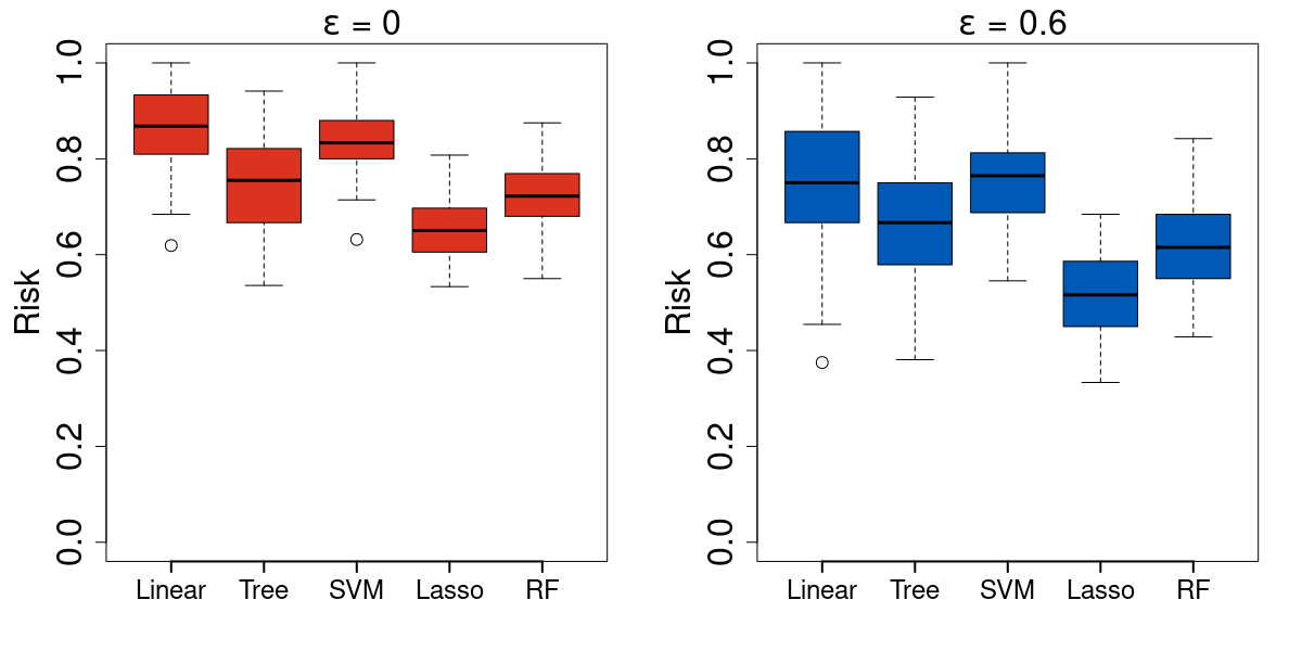
Figure 6: Estimation of $R_{\varepsilon}(g)$ for five different classifiers (cross-validation with $50$ repetitions, $70\%$ train and $30\%$ test), threshold is the $0.85$ quantile of $H$. In red (left) are the estimates when $\varepsilon=0$ and in blue (right) for $\varepsilon=0.6$. The length of the testing set is equal to $129$, this leads to around $60$ points such that $H>\varepsilon u$ and nearly $20$ points such that $H>u$.

Unlike the simulation example in Section 3.1, it is not clear to assess whether our river discharges analysis of our three selected weather stations belongs to the framework of asymptotic independence or not. Still, it is reassuring that the ranking of the classifiers in Figure 6 appears to be insensitive to the values of $R_{0}$ or $R_{\varepsilon}$. i.e. whether the data are asymptotically dependent or not. This hints that, among all the classifiers, the logistic regression with lasso penalty seems to perform better than the four other classification methods. This ranking of classifiers is specific to this particular example. No general conclusions about lasso techniques for extremes should be drawn.

Besides this river example, we advocate practitioners to compute risk functions that can both handle the asymptotic dependent and independence cases. This also complements the recent tools used to discriminate between the two cases (see, e.g. Ahmed et al.,, 2022). In addition, the linear classifier could provide a simple benchmark with well understood properties with respect to $R_{0}$, see Proposition 6.

5 Supplementary Materials

A R package is available on GitHub that implements the empirical estimation of the risk function developed in this paper (https://github.com/jlegrand35/ExtremesBinaryClassifier) and can be used either to reproduce the results of the conducted classifier comparisons or to perform new comparisons using other binary classifiers. The data used in the application are available in the R package graphicalExtremes (Engelke et al.,, 2019).

Appendix A Proofs

A.1 Proof of Lemma 1:

We can write that

$$\operatorname{\mathbb{P}}(A_{1}\cup B_{1}\mid A_{\varepsilon}\cap B_{\varepsilon}) =\frac{\operatorname{\mathbb{P}}((A_{1}\cup B_{1})\cap(A_{\varepsilon}\cap B_{\varepsilon}))}{\operatorname{\mathbb{P}}(A_{\varepsilon}\cap B_{\varepsilon})},$$

$$=\frac{\operatorname{\mathbb{P}}(A_{1}\cap B_{\varepsilon})+\operatorname{\mathbb{P}}(A_{\varepsilon}\cap B_{1})-\operatorname{\mathbb{P}}(A_{1}\cap B_{1})}{\operatorname{\mathbb{P}}(A_{\varepsilon}\cap B_{\varepsilon})}.$$

In the same way, we have

$$\operatorname{\mathbb{P}}(A_{1}\triangle B_{1}|A_{\varepsilon}\cap B_{\varepsilon}) =\frac{\operatorname{\mathbb{P}}(A_{1}\cap B_{\varepsilon})+\operatorname{\mathbb{P}}(A_{\varepsilon}\cap B_{1})-2\operatorname{\mathbb{P}}(A_{1}\cap B_{1})}{\operatorname{\mathbb{P}}(A_{\varepsilon}\cap B_{\varepsilon})}.$$

Hence, we deduce that

$$R(A_{\varepsilon},B_{\varepsilon})=\frac{\operatorname{\mathbb{P}}(A_{1}\triangle B_{1}|A_{\varepsilon}\cap B_{\varepsilon})}{\operatorname{\mathbb{P}}(A_{1}\cup B_{1}|A_{\varepsilon}\cap B_{\varepsilon})} =1-\left[\frac{\operatorname{\mathbb{P}}(A_{1}\cap B_{\varepsilon})}{\operatorname{\mathbb{P}}(A_{1}\cap B_{1})}+\frac{\operatorname{\mathbb{P}}(A_{\varepsilon}\cap B_{1})}{\operatorname{\mathbb{P}}(A_{1}\cap B_{1})}-1\right]^{-1}.$$

The expression given by (4) follows.

Item (a) of the lemma is based on the following inequality

$$\operatorname{\mathbb{P}}(U\mid V)\geq\operatorname{\mathbb{P}}(U\mid W)\mbox{, if the sets $U$, $V$ and $W$ satisfy $U\subset V\subset W$}.$$

For item (b), note that

$$R(A_{\varepsilon},B_{\varepsilon})\leq R(A^{\prime}_{\varepsilon},B_{\varepsilon})$$

$$\Longleftrightarrow\left(1-R(A_{\varepsilon},B_{\varepsilon})\right)^{-1}\leq\left(1-R(A^{\prime}_{\varepsilon},B_{\varepsilon})\right)^{-1}$$

$$\Longleftrightarrow\frac{\operatorname{\mathbb{P}}(A_{1}\cap B_{\varepsilon})}{\operatorname{\mathbb{P}}(A_{1}\cap B_{1})}+\frac{\operatorname{\mathbb{P}}(A_{\varepsilon}\cap B_{1})}{\operatorname{\mathbb{P}}(A_{1}\cap B_{1})}\leq\frac{\operatorname{\mathbb{P}}(A^{\prime}_{1}\cap B_{\varepsilon})}{\operatorname{\mathbb{P}}(A^{\prime}_{1}\cap B_{1})}+\frac{\operatorname{\mathbb{P}}(A^{\prime}_{\varepsilon}\cap B_{1})}{\operatorname{\mathbb{P}}(A^{\prime}_{1}\cap B_{1})},$$

$$\Longleftrightarrow\operatorname{\mathbb{P}}(A_{1}\cap B_{\varepsilon})+\operatorname{\mathbb{P}}(A_{\varepsilon}\cap B_{1})\leq\frac{\operatorname{\mathbb{P}}(A_{1}\cap B_{1})}{\operatorname{\mathbb{P}}(A^{\prime}_{1}\cap B_{1})}[\operatorname{\mathbb{P}}(A^{\prime}_{1}\cap B_{\varepsilon})+\operatorname{\mathbb{P}}(A^{\prime}_{\varepsilon}\cap B_{1})].$$

As $\operatorname{\mathbb{P}}(A_{1}\cap B_{1})=\operatorname{\mathbb{P}}(A^{\prime}_{1}\cap B_{1})$ and $\operatorname{\mathbb{P}}(A_{1}\cap B_{\varepsilon})=\operatorname{\mathbb{P}}(A^{\prime}_{1}\cap B_{\varepsilon})$ and $\operatorname{\mathbb{P}}(A_{\varepsilon}\cap B_{1})\leq\operatorname{\mathbb{P}}(A^{\prime}_{\varepsilon}\cap B_{1})$, then

$$R(A_{\varepsilon},B_{\varepsilon})\leq R(A^{\prime}_{\varepsilon},B_{\varepsilon}).$$

This provides the second statement (b) since we assume that $A_{1}=A^{\prime}_{1}$ and $A_{\varepsilon}\subseteq A^{\prime}_{\varepsilon}$.

Item (c) is a direct consequence of (4). $\square$

A.2 Proof of Lemma 2

First, we note that, by definition,

$$\chi^{*}(\overline{g})=c(\overline{g})\cdot\lim_{u\to\infty}\operatorname{\mathbb{P}}(H>u\mid\overline{g}(\bm{X})>u)\leq c(\overline{g}).$$

By taking the limits separately for every single term in (8), we directly obtain (9). From that, we can immediately see that

$$R(\overline{g})=0\mbox{ if and only if }1+c(\overline{g})=2\chi^{*}(\overline{g}).$$

Now, assume that $\chi^{*}(\overline{g})<c(\overline{g})$. Then, $R(\overline{g})=0$ would imply that $1+\chi^{*}(\overline{g})<2\chi^{*}(\overline{g})$ which is equivalent to $\chi^{*}(\overline{g})>1$ in contradiction to the definition of $\chi^{*}(\overline{g})$. Thus, $R(g)=0$ implies $\chi^{*}(\overline{g})=c(\overline{g})$. Plugging this into $\eqref{eq:R-xi-c}$, we obtain $c(\overline{g})=\chi^{*}(\overline{g})=1$. Conversely, $c(\overline{g})=\chi^{*}(\overline{g})=1$ obviously leads to $R(\overline{g})=0$. $\square$

A.3 Proof of Lemma 3:

From Eq. (8), we know that we can only get $R(\overline{g})<1$, only if $H$ and $\overline{g}(\bm{X})$ are tail equivalent. Thus, this will be assumed in the following. Let $w$ such that $\delta\coloneqq\lim_{u\to\infty}w(u)/u\in(0,1)$, then for any positive $u$ we can write that

$$\frac{\operatorname{\mathbb{P}}(f(\bm{X})+N>u,\overline{g}(\bm{X})>u)}{\operatorname{\mathbb{P}}(\overline{g}(\bm{X})>u)} \leq\frac{\operatorname{\mathbb{P}}(f(\bm{X})>w(u),\overline{g}(\bm{X})>u)}{\operatorname{\mathbb{P}}(\overline{g}(\bm{X})>u)}$$

$$\qquad+\frac{\operatorname{\mathbb{P}}(N>u-w(u),\overline{g}(\bm{X})>u)}{\operatorname{\mathbb{P}}(\overline{g}(\bm{X})>u)}.$$

Since $\overline{g}(\bm{X})$ and $N$ are independent, the second term reduces to $\operatorname{\mathbb{P}}(N>u-w(u))$ which converges to $0$ since $u-w(u)\sim(1-\delta)u$ as $u$ gets large.

For the first term, we rewrite the ratio as follows

$$\frac{\operatorname{\mathbb{P}}(f(\bm{X})>w(u),\overline{g}(X)>u)}{\operatorname{\mathbb{P}}(\overline{g}(\bm{X})>u)} \leq\frac{\operatorname{\mathbb{P}}(f(\bm{X})>w(u))}{\operatorname{\mathbb{P}}(\overline{g}(\bm{X})>u)}$$

$$\leq\frac{\operatorname{\mathbb{P}}(f(\bm{X})>w(u))}{\operatorname{\mathbb{P}}(N>w(u))}\frac{\operatorname{\mathbb{P}}(N>w(u))}{\operatorname{\mathbb{P}}(N>u)}\frac{\operatorname{\mathbb{P}}(N>u)}{\operatorname{\mathbb{P}}(\overline{g}(\bm{X})>u)}.$$

Since $w(u)\to\infty$ and $\operatorname{\mathbb{P}}(f(\bm{X})>u)=o\left(\operatorname{\mathbb{P}}(N>u)\right)$, the ratio $\frac{\operatorname{\mathbb{P}}(f(\bm{X})>w(u))}{\operatorname{\mathbb{P}}(N>w(u))}$ goes to $0$ as $u$ gets large. From the assumption $w(u)\sim\delta u$, $\frac{\operatorname{\mathbb{P}}(N>w(u))}{\operatorname{\mathbb{P}}(N>u)}$ behaves as a constant when $u\to\infty$.

The only remaining term is $\frac{\operatorname{\mathbb{P}}(N>u)}{\operatorname{\mathbb{P}}(\overline{g}(\bm{X})>u)}$ which converges to a constant due to tail equivalence. So, $\lim\operatorname{\mathbb{P}}(\overline{g}(\bm{X})>u\mid H>u)=0$. $\square$

A.4 Proof of Proposition 4:

In Lemma 1 we fix $A_{\varepsilon}=\{\overline{g}(\bm{X})>\varepsilon u\}$ and $B_{\varepsilon}=\{H>\varepsilon u\}$ and $A_{1}=\{\overline{g}(\bm{X})>u\}$ and $B_{1}=\{H>u\}$.

$$\operatorname{\mathbb{P}}(H>u\text{ or }\overline{g}(\bm{X})>u\mid\min\{H,\overline{g}(\bm{X})\}>\varepsilon u)=\operatorname{\mathbb{P}}(A_{1}\cup B_{1}\mid A_{\varepsilon}\cap B_{\varepsilon}),$$

and

$$\operatorname{\mathbb{P}}(g(\bm{X};u)\neq Y^{(u)}\mid\min\{H,\overline{g}(\bm{X})\}>\varepsilon u)=\operatorname{\mathbb{P}}(A_{1}\triangle B_{1}|A_{\varepsilon}\cap B_{\varepsilon}).$$

The Ramos and Ledford model corresponds to the special of case of (5)

$$\operatorname{\mathbb{P}}[\overline{g}(\bm{X})>\varepsilon u,H>\varepsilon^{\prime}u]=L(\varepsilon u,\varepsilon^{\prime}u)((\varepsilon u)^{-\alpha_{g}}(\varepsilon^{\prime}u)^{-\alpha_{H}})^{1/2\eta}=\operatorname{\mathbb{P}}(A_{\varepsilon}\cap B_{\varepsilon^{\prime}})=c_{\varepsilon,\varepsilon^{\prime}}\operatorname{\mathbb{P}}^{a}(A_{\varepsilon})\operatorname{\mathbb{P}}^{b}(B_{\varepsilon^{\prime}})$$

with

$$\operatorname{\mathbb{P}}(A_{\varepsilon}) =\operatorname{\mathbb{P}}(\overline{g}(X)>\varepsilon u)=L_{g}(\varepsilon u)\varepsilon^{-\alpha_{g}}u^{-\alpha_{g}},$$

$$\operatorname{\mathbb{P}}(B_{\varepsilon}) =\operatorname{\mathbb{P}}(H>\varepsilon u)=L_{H}(\varepsilon u)\varepsilon^{-\alpha_{H}}u^{-\alpha_{H}}$$

and

$$c_{\varepsilon,\varepsilon^{\prime}}=\frac{L(\varepsilon u,\varepsilon^{\prime}u)}{(L_{g}(\varepsilon u)L_{H}(\varepsilon^{\prime}u))^{1/(2\eta)}},\quad a=b=\frac{1}{2\eta}.$$

Then, from (6)

$$R(A_{\varepsilon},B_{\varepsilon})=1-\left[\frac{c_{\varepsilon,1}}{c_{1,1}}(\operatorname{\mathbb{P}}(A_{1}|A_{\varepsilon}))^{-a}+\frac{c_{1,\varepsilon}}{c_{1,1}}(\operatorname{\mathbb{P}}(B_{1}|B_{\varepsilon}))^{-b}-1\right]^{-1}.$$

Letting $u$ gets large provides the required result. $\square$.

A.5 Proof of Proposition 5:

As we assume that $R_{\varepsilon}(g)$ exists (for some $\varepsilon\geq 0$), for $u_{n}\to\infty$ such that $np_{g,\varepsilon}(u_{n})\to\infty$, we obtain that

$$\sqrt{np_{g,\varepsilon}(u_{n})}\Biggl{[}\begin{pmatrix}\frac{\sum_{i=1}^{n}\mathds{1}\{g(\bm{X}_{i},u_{n})\neq Y^{(u_{n})}_{i},H_{i}>\varepsilon u_{n},g(\bm{X}_{i};\varepsilon u_{n})=1\}}{np_{g,\varepsilon}(u_{n})}\\ \frac{\sum_{i=1}^{n}\mathds{1}\{\max\{g(\bm{X}_{i},u_{n}),Y^{(u_{n})}_{i}\}=1,H_{i}>\varepsilon u_{n},g(\bm{X}_{i};\varepsilon u_{n})=1\}}{np_{g,\varepsilon}(u_{n})}\end{pmatrix}$$

$$-\begin{pmatrix}\frac{\operatorname{\mathbb{P}}(g(\bm{X},u_{n})\neq Y^{(u_{n})},H>\varepsilon u_{n},g(\bm{X};\varepsilon u_{n})=1)}{p_{g,\varepsilon}(u_{n})}\\ 1\end{pmatrix}\Biggr{]}$$

$$\stackrel{{\scriptstyle n\to\infty}}{{\longrightarrow}}\mathcal{N}\left(\begin{pmatrix}0\\ 0\end{pmatrix},\begin{pmatrix}R_{\varepsilon}(g)&R_{\varepsilon}(g)\\ R_{\varepsilon}(g)&1\end{pmatrix}\right)$$

Provided that the bias is negligible, i.e.

$$\lim_{n\to\infty}\sqrt{np_{g,\varepsilon}(u_{n})}\left(\frac{\operatorname{\mathbb{P}}(g(\bm{X},u_{n})\neq Y^{(u_{n})},H>\varepsilon u_{n},g(\bm{X};\varepsilon u_{n})=1)}{p_{g,\varepsilon}(u_{n})}-R_{\varepsilon}(g)\right)=0,$$

the Delta method yields

$$\sqrt{np_{g,\varepsilon}(u_{n})}\left(\widehat{R}_{n,\varepsilon}(g)-R_{\varepsilon}(g)\right)\stackrel{{\scriptstyle n\to\infty}}{{\longrightarrow}}\mathcal{N}\left(0,R_{\varepsilon}(g)(1-R_{\varepsilon}(g))\right).$$

$\square$

Appendix B Linear Classifiers

B.1 Definition, Basic Properties and Inference

In this section, we consider a specific type of classifiers which in this paper is referred to as linear classifiers, i.e. classifiers of the form

$$g_{\bm{\theta}}(\bm{X};u)=\begin{cases}+1,&\quad\bm{\theta}^{\top}\bm{X}>u,\\ -1,&\quad\bm{\theta}^{\top}\bm{X}\leq u,\end{cases}\qquad\bm{\theta}\in[0,\infty)^{d}.$$

To obtain an optimal linear classifier of $g_{\bm{\theta}}(\bm{X};u)$, i.e. some weight vector $\bm{\theta}^{*}$ such that the classification risk $R(g_{\bm{\theta}^{*}})$ gets minimal, we need to impose some joint extremal dependence structure on $\bm{X}$ and $H$ from (2).

Even though some of the results can also be obtained in a similar manner in a more general framework for the conditional risk $R_{\varepsilon}$, henceforth, we will focus on the asymptotically dependent case where we might find some optimal classifier with unconditional risk $R(g_{\bm{\theta}^{*}})<1$. As discussed before, in this case, at least one component of $\bm{X}$ needs to have a similar tail behavior as $H$. A natural assumption is therefore that $(\bm{X},H)$ is jointly regularly varying on $[0,\infty)$ with index $\alpha>0$, i.e. there exist an $\alpha$-Pareto random variable $P$ and, independently of $P$, a random vector $(\bm{\Gamma},\Omega)\in[0,\infty)^{d}\times[0,\infty)$, the so-called spectral tail vector, on the unit sphere $\{\bm{x}\in[0,\infty)^{d+1}:\,\|\bm{x}\|_{\infty}=1\}$ such that

$$\mathcal{L}\left(\left(\frac{\|(\bm{X},H)\|_{\infty}}{u},\frac{(\bm{X},H)}{\|(\bm{X},H)\|_{\infty}}\right)\,\bigg{|}\,\|(\bm{X},H)\|_{\infty}>u\right)\to_{w}\mathcal{L}(P,(\bm{\Gamma},\Omega)),\mbox{as }u\to\infty.$$

Here, we additionally assume that  $\operatorname{\mathbb{P}}(\|\bm{\Gamma}\|_{\infty}>0)>0$ and $\operatorname{\mathbb{P}}(\Omega>0)>0$. In this setup,  $\|\bm{X}\|_{\infty}$ and $H$ are tail equivalent in the sense that

$$\lim_{u\to\infty}\frac{\operatorname{\mathbb{P}}(\|\bm{X}\|_{\infty}>u)}{\operatorname{\mathbb{P}}(H>u)}={} \lim_{u\to\infty}\frac{\operatorname{\mathbb{P}}(\|\bm{X}\|_{\infty}>u\mid\|(\bm{X},H)\|_{\infty}>u)}{\operatorname{\mathbb{P}}(H>u\mid\|(\bm{X},H)\|_{\infty}>u)}$$

$$={} \frac{\operatorname{\mathbb{P}}(P\cdot\|\bm{\Gamma}\|_{\infty}>1)}{\operatorname{\mathbb{P}}(P\cdot\Omega>1)}=\frac{\operatorname{\mathbb{E}}(\|\bm{\Gamma}\|_{\infty}^{\alpha})}{\operatorname{\mathbb{E}}(\Omega^{\alpha})}\in(0,\infty),$$

This is the minimal requirement on the link between the covariates $\bm{X}$ and the unobserved extremes of $H$ essentially saying that at least one component of $\bm{X}$ is tail-equivalent to $H$. It is important to highlight that we do not exclude the case that $\Gamma_{i}=0$ a.s. for some $i\in\{1,\ldots,d\}$ which means that $X_{i}$ possesses a lighter tail than $H$. This property can be read off from the quantity

$$c_{i}=\lim_{u\to\infty}\frac{\operatorname{\mathbb{P}}(X_{i}>u)}{\operatorname{\mathbb{P}}(H>u)}=\frac{\operatorname{\mathbb{E}}(\Gamma_{i}^{\alpha})}{\operatorname{\mathbb{E}}(\Omega^{\alpha})}.$$

Thus, $\Gamma_{i}=0$ a.s. if and only if $c_{i}=0$. By including this case, we therefore admit that most of the components of $\bm{X}$ may not contribute to the extremes of the vector $H$.

Under these conditions, we obtain that, for all $\bm{\theta}\in[0,\infty)^{d}$, the classifier $g_{\bm{\theta}}$ is an extremal classifier as

$$R(g_{\bm{\theta}})={} \lim_{u\to\infty}\operatorname{\mathbb{P}}(H>u\text{ or }g(\bm{X})>u)^{-1}\left(\operatorname{\mathbb{P}}[\max\{\bm{\theta}^{\top}\bm{X},H\}>u]-\operatorname{\mathbb{P}}[\min\{\bm{\theta}^{\top}\bm{X},H\}>u]\right)$$

$$={} \frac{\operatorname{\mathbb{E}}\left(\max\{\bm{\theta}^{\top}\bm{\Gamma},\Omega\}^{\alpha}\right)-\operatorname{\mathbb{E}}\left(\min\{\bm{\theta}^{\top}\bm{\Gamma},\Omega\}^{\alpha}\right)}{\operatorname{\mathbb{E}}\left(\max\{\bm{\theta}^{\top}\bm{\Gamma},\Omega\}^{\alpha}\right)}{}={}1-\frac{\operatorname{\mathbb{E}}\left(\min\{\bm{\theta}^{\top}\bm{\Gamma},\Omega\}^{\alpha}\right)}{\operatorname{\mathbb{E}}\left(\max\{\bm{\theta}^{\top}\bm{\Gamma},\Omega\}^{\alpha}\right)}\in[0,1].$$ (15)

Equation (B.1) implies that the function $\bm{\theta}\mapsto R(g_{\bm{\theta}})$ is well-defined and continuous on $[0,\infty)^{d}$. Its value does not depend on those components $\theta_{i}$ for which $\Gamma_{i}=0$ a.s., which is equivalent to $c_{i}=0$ as discussed above. Thus, in the following, we will consider this function only on the parameter set

$$C=\{\bm{\theta}\in[0,\infty)^{d}:\theta_{i}=0\text{ for all $i$ s.t. }c_{i}=0\},$$

containing all the relevant information – here, note that, in practice, identifying the components $i\in\{1,\ldots,d\}$ such that $c_{i}=0$ a.s., from a given data set is a necessary step for the correct specification of the set $C$.

From the consideration in the introduction, it can be easily seen that $R(g_{\bm{0}})=1$ – the case $\bm{\theta}=\bm{0}$ corresponds to the trivial always optimistic classifier. Furthermore, denoting the set of indices $j$ with $c_{j}>0$ by $J$, we can see that

$$R(g_{\bm{\theta}})\geq 1-\frac{\operatorname{\mathbb{E}}(\Omega^{\alpha})}{\|\bm{\theta}\|^{\alpha}_{\infty}\cdot\min_{j\in J}\operatorname{\mathbb{E}}(\Gamma_{j}^{\alpha})}\to 1$$ (16)

as $\|\bm{\theta}\|_{\infty}\to\infty$. By the continuity of $\bm{\theta}\mapsto R(g_{\bm{\theta}})$, we obtain that the function attains a global minimum on the domain $C$.

Proposition 6

Additionally to the assumptions above on the joint distribution of $(\bm{X},H)$ with $\alpha>1$, assume that there exists a function $a(u)$ with $a(u)\to 0$ as $u\to\infty$ such that

$$\operatorname{\mathbb{P}}(u^{-1}\bm{X}\in A\mid\|(\bm{X},H)\|>u)\leq(1+a(u))\operatorname{\mathbb{P}}(P\bm{\Gamma}\in A)$$ (17)

for all $A\subset[0,\infty)$. Furthermore, let $u_{n}\to\infty$ and $n\operatorname{\mathbb{P}}(H>u_{n})\to\infty$ such that, for every compact subset $K\subset C$,

$$\sup_{\bm{\theta}\in K}\sqrt{n\operatorname{\mathbb{P}}(H>u_{n})}\left|\frac{\operatorname{\mathbb{P}}(g_{\bm{\theta}}(\bm{X};u_{n})\neq Y^{u_{n}})}{\operatorname{\mathbb{P}}(H>u_{n})}-\frac{\operatorname{\mathbb{E}}\left(\max\{\bm{\theta}^{\top}\bm{\Gamma},\Omega\}^{\alpha}\right)-\operatorname{\mathbb{E}}\left(\min\{\bm{\theta}^{\top}\bm{\Gamma},\Omega\}^{\alpha}\right)}{\operatorname{\mathbb{E}}(\Omega^{\alpha})}\right|={} 0$$ (18)

and

$$\sup_{\bm{\theta}\in K}\sqrt{n\operatorname{\mathbb{P}}(H>u_{n})}\left|\frac{\operatorname{\mathbb{P}}(\max\{g_{\bm{\theta}}(\bm{X};u_{n}),Y^{u_{n}}\}=1)}{\operatorname{\mathbb{P}}(H>u_{n})}-\frac{\operatorname{\mathbb{E}}\left(\max\{\bm{\theta}^{\top}\bm{\Gamma},\Omega\}^{\alpha}\right)}{\operatorname{\mathbb{E}}(\Omega^{\alpha})}\right|={} 0.$$ (19)

If the function $\bm{\theta}\mapsto R(g_{\bm{\theta}})$ has a unique minimizer $\bm{\theta}^{*}$ in $C$, then the estimator

$$\hat{\bm{\theta}}_{n,u_{n}}=\mathop{\mathrm{argmin}}_{\bm{\theta}\in C}\hat{R}_{n}(g_{\bm{\theta}}(\cdot;u_{n})).$$

is consistent, i.e. $\hat{\bm{\theta}}_{n,u_{n}}\to_{p}\bm{\theta}^{*}$.

Given the set $C$, this result provides a strategy to find the optimal $\bm{\theta}$, i.e., the best linear classifier. Determining the set $C$ requires the identification of the relevant features, i.e. the index set $J$ such that $c_{j}>0$ if and only if $j\in J$. This is discussed in more detail in the following subsection.

B.2 Feature Selection

The notion of sparsity quickly comes into play when doing classification. This is all the more true when one is only interested in the extremes. Among the whole data set, only a small proportion will truly contribute to the extremal behavior of the variable of interest. Here, we develop a method to identify the informative signals in terms of extremes among a large data set, assuming that $(\bm{X},H)$ is jointly regularly varying. For a comprehensive review of existing methods on sparsity and multivariate extremes we highly recommend the work of Engelke and Ivanovs, (2021).

As we have seen above, for linear classifiers, all the relevant features $X_{i}$ necessarily satisfy $c_{i}>0$. Thus, feature selection can be based on estimation of the $c_{i}$ which can be done according to the following proposition.

Proposition 7

Assume that

$$c_{i}=\lim_{u\to\infty}\frac{\operatorname{\mathbb{P}}(X_{i}>u)}{\operatorname{\mathbb{P}}(H>u)}$$

exists. If $u_{n}\to\infty$ and $n\operatorname{\mathbb{P}}(H>u_{n})\to\infty$, then

$$\frac{\sum_{j=1}^{n}\mathbf{1}\{X_{j,i}>u_{n}\}}{\sum_{j=1}^{n}\mathbf{1}\{H_{j}>u_{n}\}}\to_{p}c_{i}.$$

If, additionally,

$$\sqrt{n\operatorname{\mathbb{P}}(H>u_{n})}\left(\frac{\operatorname{\mathbb{P}}(X_{i}>u_{n})}{\operatorname{\mathbb{P}}(H>u_{n})}-c_{i}\right)\to 0$$

and

$$\chi_{i}^{*}=\lim_{u\to\infty}\operatorname{\mathbb{P}}(X_{i}>u\mid H>u)\in[0,1]$$

exists, then, we have

$$\sqrt{n\operatorname{\mathbb{P}}(H>u_{n})}\left(\frac{\sum_{j=1}^{n}\mathbf{1}\{X_{j,i}>u_{n}\}}{\sum_{j=1}^{n}\mathbf{1}\{H_{j}>u_{n}\}}-c_{i}\right)\to\mathcal{N}\left(0,c_{i}\cdot\left[1-2\chi^{*}_{i}+c_{i}\right]\right).$$

Appendix C River network

This section deals with a simpler case than the application in Section 4. Here an application could be the following: we want to know which stations should continue to be maintained to prevent extreme floods and maybe some stations are not necessary.

Here we still want to predict the extreme events at station 1. We define an extreme event as an event exceeding the $85th$ quantile of $X_{1}$ and we assume that the whole set of remaining stations is available. In this case, strong dependencies among station 1 and other stations can be observed. So, the main issue is to select these stations following the procedure presented in Appendix B.

As in the simulated study, we identify the stations that may not contribute to the extremes of $X_{1}$ by estimating the $c_{i}$. The estimation of the set $C$ on all the data is presented in Table 2. We found that among the 30 stations, only three stations are relevant: stations 2, 13 and 30. Looking at Figure 4, these stations correspond to the stations closest to $X_{1}$. Figure 7 shows the scatter plots between these stations and station 1.

Table 2: Empirical estimates of $\hat{c}_{i}$ (as defined in proposition 7) for each station. The values different from zero are highlighted in red.

	$c_{i}$
X2	0.06
X3	0.00
X4	0.00
X5	0.00
X6	0.00
X7	0.00
X8	0.00
X9	0.00
X10	0.00
X11	0.00
X12	0.00
X13	0.30
X14	0.00
X15	0.00
X16	0.00

	$c_{i}$
X17	0.00
X18	0.00
X19	0.00
X20	0.00
X21	0.00
X22	0.00
X23	0.00
X24	0.00
X25	0.00
X26	0.00
X27	0.00
X28	0.00
X29	0.00
X30	0.02
X31	0.00

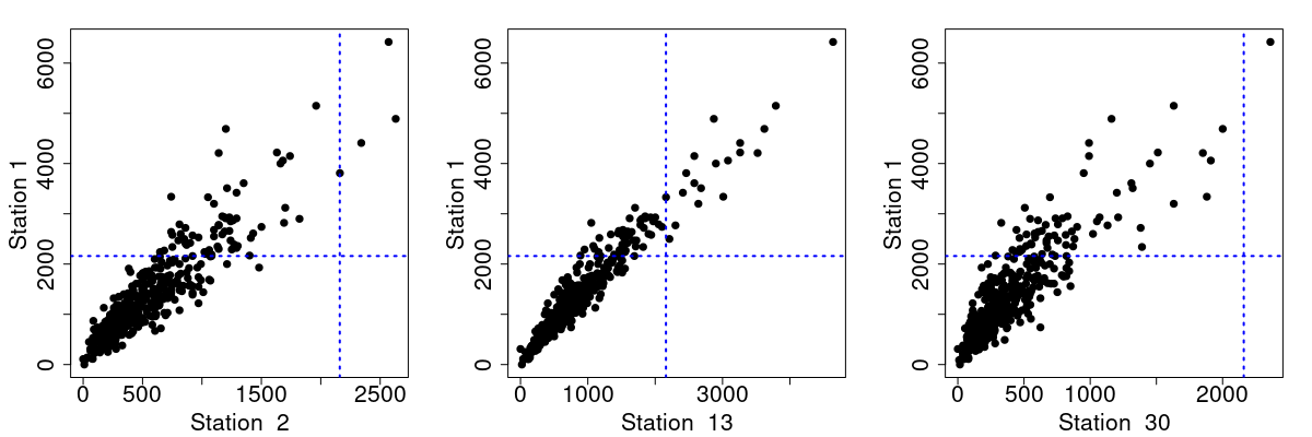
Figure 7: Correlation plot between $X_{1}$ and the stations considered to contribute to the extremes of $X_{1}$ according to the table 2 (i.e. for which $c_{i}\neq 0$). The blue dotted lines represent the threshold $u$ defined by the $85$th percentile of $X_{1}$.

Once the contributing variables have been identified, we compare the performance of several classifiers, on the one hand keeping all the data and on the other hand keeping only the informative stations. Since there is a strong dependence between the data, we assume that it is sufficient here to look at the risk $R_{0}$. Comparison results are shown in Figure 8.

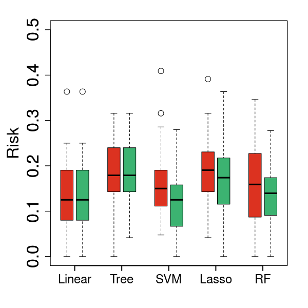
Figure 8: Estimation of $R_{0}(g)$ for different classifiers $g$ (cross-validation - $70\%$ train, $30\%$ test - with $50$ repetitions). The red distributions come from the estimation with all the stations, and the green distributions represent the estimations with only the variables having $\hat{c}_{i}\neq 0$.

By definition of the linear classifier, the estimation is already done by keeping only the informative variables, which is why the estimates are identical for this specific classifier. As for the other classifiers, we see some improvements when keeping only the informative variables: the risk estimates are slightly smaller. This means that even if we remove a lot of information by going from 30 explanatory variables to 3, these 3 remaining stations contain all the information in terms of extremes of station 1.

Appendix D Proofs of the appendix

D.1 Proof of Proposition 6

The proof is based on the following lemma which is proven in Subsection D.2.

Lemma 8

Under the assumptions from Proposition 6, for every compact subset $K\subset C$, the sequences of processes $\{A_{n}(\bm{\theta}),\,\bm{\theta}\in K\}$ and $\{B_{n}(\bm{\theta}),\,\bm{\theta}\in K\}$ defined by

$$A_{n}(\bm{\theta})={} \sqrt{\frac{n}{\operatorname{\mathbb{P}}(H>u_{n})}}\left(\frac{1}{n}\sum_{i=1}^{n}\mathds{1}\Big{\{}\{\bm{\theta}^{\top}\bm{X}_{i}>u_{n}\}\triangle\{H_{i}>u_{n}\}\Big{\}}-\operatorname{\mathbb{P}}(g_{\bm{\theta}}(\bm{X};u_{n})\neq Y^{(u_{n})})\right)$$

$$B_{n}(\bm{\theta})={} \sqrt{\frac{n}{\operatorname{\mathbb{P}}(H>u_{n})}}\left(\frac{1}{n}\sum_{i=1}^{n}\mathds{1}\Big{\{}\{\bm{\theta}^{\top}\bm{X}_{i}>u_{n}\}\cup\{H_{i}>u_{n}\}\big{\}}-\operatorname{\mathbb{P}}(\max\{g_{\bm{\theta}}(\bm{X};u_{n}),Y^{(u_{n})}\}=1)\right)$$

converge to centered Gaussian processes $\{A(\bm{\theta}),\ \bm{\theta}\in K\}$ and $\{B(\bm{\theta}),\ \bm{\theta}\in K\}$, respectively, weakly in $\ell^{\infty}(K)$.

If the function $\bm{\theta}\mapsto R(g_{\bm{\theta}})$ has a unique minimizer $\bm{\theta}^{*}$, then, necessarily, $R(g_{\bm{\theta}^{*}})<1$.
Now, similarly to the notation above, let $J$ denote the set of indices $j$ with $c_{j}>0$, and let us consider $\bm{\theta}\in C$ such that $\|\bm{\theta}\|_{\infty}>k_{0}$ for some constant $k_{0}>0$. Then,

$$\widehat{R}_{n}(g_{\bm{\theta}})={} 1-\frac{\sum_{i=1}^{n}\mathds{1}\{\min(\bm{\theta}^{\top}\bm{X}_{i},H_{i}\}>u_{n})\}}{\sum_{i=1}^{n}\mathds{1}\{\max(\bm{\theta}^{\top}\bm{X}_{i},H_{i}\}>u_{n})\}}\geq 1-\frac{\sum_{i=1}^{n}\mathds{1}\{H_{i}>u_{n}\}}{\min_{j\in J}\sum_{i=1}^{n}\mathds{1}\{k_{0}X_{ij}>u_{n}\}}$$

$$\stackrel{{\scriptstyle n\to\infty}}{{\longrightarrow}}_{p}{} 1-\max_{j\in J}\frac{\operatorname{\mathbb{E}}(\Omega^{\alpha})}{k_{0}^{\alpha}\operatorname{\mathbb{E}}(\Gamma_{j}^{\alpha})}$$

where the right-hand side goes to $1$ as $k_{0}\to\infty$. Thus, as $\widehat{R}_{n}(g_{\bm{\theta}^{*}})\to_{p}R(g_{\bm{\theta}^{*}})<1$, we obtain that, for sufficiently large $k_{0}\gg\|\bm{\theta}^{*}\|$, with probability going to one,

$$\widehat{R}_{n}(g_{\bm{\theta}^{*}})\leq\min_{\bm{\theta}\in C\setminus[0,k_{0}]^{d}}\widehat{R}_{n}(g_{\bm{\theta}})$$

and, consequently,

$$\mbox{argmin}_{\bm{\theta}\in C}\widehat{R}_{n}(g_{\bm{\theta}})={} \mbox{argmin}_{\bm{\theta}\in C\cap[0,k_{0}]^{d}}\widehat{R}_{n}(g_{\bm{\theta}}).$$

Now, we note that, by Lemma 8, the bias conditions (18) and (19) and the functional delta method, $\widehat{R}_{n}(g_{\bm{\theta}})$ converges in probability to $R(g_{\bm{\theta}})$ uniformly on every compact subset of $C$. In particular,

$$\sup_{\bm{\theta}\in C\cap[0,K]^{d}}\left|\widehat{R}_{n}(g_{\bm{\theta}})-R(g_{\bm{\theta}})\right|\to_{p}0.$$

Thus,

$$\mbox{argmin}_{\bm{\theta}\in C\cap[0,K]^{d}}\widehat{R}_{n}(g_{\bm{\theta}})\to_{p}\mbox{argmin}_{\bm{\theta}\in C\cap[0,K]^{d}}R(g_{\bm{\theta}})=\bm{\theta}^{*}.$$

$\square$

D.2 Proof of Lemma 8

We will proof the lemma by applying the Central Limit Theorem 2.11.9 in Van der Vaart and Wellner, (1996). To this end, we define the function spaces $\mathcal{A}=\{a_{\bm{\theta}},\ \bm{\theta}\in K\}$ and $\mathcal{B}=\{b_{\bm{\theta}},\ \bm{\theta}\in K\}$ where

$$a_{\bm{\theta}}:(0,\infty)^{d}\times(0,\infty)\to\{0,1\}, \quad a_{\bm{\theta}}(\bm{x},h)=\mathds{1}\Big{\{}\{\bm{\theta}^{\top}\bm{x}>1\}\triangle\{h>1\}\big{\}}$$

$$b_{\bm{\theta}}:(0,\infty)^{d}\times(0,\infty)\to\{0,1\}, \quad b_{\bm{\theta}}(\bm{x},h)=\mathds{1}\Big{\{}\{\bm{\theta}^{\top}\bm{x}>1\}\cup\{h>1\}\big{\}}.$$

Then, with

$$Z_{nl}(f)=\frac{1}{\sqrt{n\operatorname{\mathbb{P}}(H>u_{n})}}f(u_{n}^{-1}\bm{X}_{l},u_{n}^{-1}H_{l}),\quad f\in\mathcal{A}\cup\mathcal{B},$$

for $l=1,\ldots,n,$ we have that

$$\{A_{n}(\bm{\theta}),\ \bm{\theta}\in K\}=\left\{\sum\nolimits_{l=1}^{n}(Z_{nl}(f)-\operatorname{\mathbb{E}}Z_{nl}(f)),\ f\in\mathcal{A}\right\}$$

and

$$\{B_{n}(\bm{\theta}),\ \bm{\theta}\in K\}=\left\{\sum\nolimits_{l=1}^{n}(Z_{nl}(f)-\operatorname{\mathbb{E}}Z_{nl}(f)),\ f\in\mathcal{B}\right\}.$$

Now, we have that

$$\max\left\{\|Z_{nl}\|_{\mathcal{A}},\|Z_{nl}\|_{\mathcal{B}}\right\}=\sup_{f\in\mathcal{A}\cup\mathcal{B}}|Z_{nl}(f)|\leq\frac{1}{\sqrt{n\operatorname{\mathbb{P}}(H>u_{n})}}\ \text{a.s.}$$

for all $l=1,\ldots,n$ and $n\in\mathbb{N}$.
Consequently, we check the Lindeberg condition: For $k\in\mathbb{N}$, we have

$$\lim_{n\to\infty}\sum_{l=1}^{n}\operatorname{\mathbb{E}}\left(\|Z_{nl}\|^{k}_{\mathcal{A}\cup\mathcal{B}}\mathds{1}\{\|Z_{nl}\|_{\mathcal{A}\cup\mathcal{B}}>\eta\}\right)\leq\lim_{n\to\infty}\frac{n}{\sqrt{n\operatorname{\mathbb{P}}(H>u_{n})}^{k}}\mathds{1}\{n\operatorname{\mathbb{P}}(H>u_{n})<1/\eta^{2}\}=0$$

as $n\operatorname{\mathbb{P}}(H>u_{n})\to\infty$ by definition. For $k=2$, we obtain a Lindeberg type condition that ensures convergence of $A_{n}$ and $B_{n}$ to $A$ and $B$, respectively, in terms of finite-dimensional distributions. For $k=1$, we obtain the Lindeberg type condition of Theorem 2.11.9 in Van der Vaart and Wellner, (1996).

It remains to check the equi-continuity condition. In the following, to simplify notation, we assume that $C=[0,\infty)^{d}$. Then, for $\theta^{(1)},\theta^{(2)}\in[a,b]\subset K\subset C$, we have that

$$|a_{\theta^{(1)}}(u_{n}^{-1}\bm{X},u_{n}^{-1}H)-a_{\theta^{(2)}}(u_{n}^{-1}\bm{X},u_{n}^{-1}H)|\in\{0,1\}$$

and

$$|b_{\theta^{(1)}}(u_{n}^{-1}\bm{X},u_{n}^{-1}H)-b_{\theta^{(2)}}(u_{n}^{-1}\bm{X},u_{n}^{-1}H)|\in\{0,1\}$$

and the probability that any of those two expressions is equal to one is bounded by the probability

$$\operatorname{\mathbb{P}}(\mathds{1}\{a^{\top}\bm{X}>u_{n}\}\neq\mathds{1}\{b^{\top}\bm{X}>u_{n}\})={}\operatorname{\mathbb{P}}(a^{\top}\bm{X}\leq u_{n},b^{\top}\bm{X}>u_{n})$$

$$={} \operatorname{\mathbb{P}}\left(\|(\bm{X},H)\|>\frac{u_{n}}{\|K\|d}\right)\operatorname{\mathbb{P}}\left(a^{\top}\bm{X}\leq u_{n},b^{\top}\bm{X}>u_{n}\,\Big{|}\,\|(\bm{X},H)\|>\frac{u_{n}}{\|K\|d}\right)$$

where we use that $b^{\top}\bm{X}>u_{n}$ implies that $\|X\|>u_{n}/(\|K\|d)$ with $\|K\|=\sup_{x\in K}\|x\|_{\infty}$. Making use of the fact that $\operatorname{\mathbb{P}}\left(\|(\bm{X},H)\|>u_{n}/(\|K\|d)\right)\leq C_{0}(\|K\|d)^{\alpha}\operatorname{\mathbb{P}}(H>u_{n})$ for some constant $C_{0}>0$ and the bound given by Equation (17), we obtain that

$$\operatorname{\mathbb{P}}(\mathds{1}\{a^{\top}\bm{X}>u_{n}\}\neq\mathds{1}\{b^{\top}\bm{X}>u_{n}\})$$

$$\leq{} C_{0}(\|K\|d)^{\alpha}\operatorname{\mathbb{P}}(H>u_{n})[1+a(u_{n}/(\|K\|d))]\operatorname{\mathbb{P}}\left(Pa^{\top}\bm{\Gamma}\leq\|K\|d,Pb^{\top}\bm{\Gamma}>\|K\|d\right)$$

$$={} C_{0}(\|K\|d)^{\alpha}\operatorname{\mathbb{P}}(H>u_{n})[1+a(u_{n}/(\|K\|d))]\operatorname{\mathbb{E}}_{\bm{\Gamma}}\left(\operatorname{\mathbb{P}}\left(P\in\left[\frac{\|K\|d}{b^{\top}\bm{\Gamma}},\frac{\|K\|d}{a^{\top}\bm{\Gamma}}\right]\right)\right)$$

$$\leq{} C_{0}\operatorname{\mathbb{P}}(H>u_{n})[1+a(u_{n}/(\|K\|d))]\operatorname{\mathbb{E}}\left((b^{\top}\bm{\Gamma})^{\alpha}-(a^{\top}\Gamma)^{\alpha}\right)$$

$$\leq{} 2C_{0}\operatorname{\mathbb{P}}(H>u_{n})\|a-b\|$$

provided that $u_{n}$ is sufficiently large as $a(u_{n}/(\|K\|d))\to 0$.

Consequently,

$$\sup_{\|f-g\|<\delta}\sum_{l=1}^{n}\operatorname{\mathbb{E}}\left[(Z_{nl}(f)-Z_{nl}(g))^{2}\right]=2C_{0}\delta,$$

which tends to $0$ as $\delta\to 0$. From this inequality, it can also be seen that any partition of $K$ into hypercubes with length $\varepsilon^{2}/(2C_{0})$ leads to a valid $\varepsilon$-bracketing, i.e. the number $N_{\varepsilon}\propto 1/\varepsilon^{2d}$ grows with a power rate and, so, $\sqrt{\log(N_{\varepsilon})}$ is integrable.

Thus, by Theorem 2.11.9, the processes $A_{n}$ and $B_{n}$ converge to Gaussian processes $A$ and $B$, weakly in $\ell^{\infty}(K)$. $\square$

References

- Aghbalou et al., (2021) Aghbalou, A., Portier, F., Sabourin, A., and Zhou, C. (2021). Tail inverse regression for dimension reduction with extreme response. arXiv:2108.01432.
- Ahmed et al., (2022) Ahmed, M., Maume-Deschamps, V., and Ribereau, P. (2022). Recognizing a spatial extreme dependence structure: A deep learning approach. Environmetrics, 33(4):e2714.
- Asadi et al., (2015) Asadi, P., Davison, A. C., and Engelke, S. (2015). Extremes on river networks. The Annals of Applied Statistics, 9(4):2023 – 2050.
- Coles et al., (1999) Coles, S., Heffernan, J., and Tawn, J. (1999). Dependence measures for extreme value analyses. Extremes, 2:339–365.
- Engelke et al., (2019) Engelke, S., Hitz, A. S., and Gnecco, N. (2019). graphicalExtremes: Statistical Methodology for Graphical Extreme Value Models. R package version 0.1.0.9000.
- Engelke and Ivanovs, (2021) Engelke, S. and Ivanovs, J. (2021). Sparse structures for multivariate extremes. Annual Review of Statistics and Its Application, 8(1):241–270.
- Ferro, (2007) Ferro, C. A. T. (2007). A probability model for verifying deterministic forecasts of extreme events. Weather and Forecasting, 22(5):1089 – 1100.
- Ferro and Stephenson, (2011) Ferro, C. A. T. and Stephenson, D. B. (2011). Extremal dependence indices: Improved verification measures for deterministic forecasts of rare binary events. Weather and Forecasting, 26(5):699 – 713.
- Gnecco et al., (2021) Gnecco, N., Meinshausen, N., Peters, J., and Engelke, S. (2021). Causal discovery in heavy-tailed models. The Annals of Statistics, 49(3):1755 – 1778.
- Gneiting et al., (2007) Gneiting, T., Balabdaoui, F., and Raftery, A. E. (2007). Probabilistic forecasts, calibration and sharpness. Journal of the Royal Statistical Society: Series B (Statistical Methodology), 69(2):243–268.
- Haixiang et al., (2017) Haixiang, G., Yijing, L., Shang, J., Mingyun, G., Yuanyue, H., and Bing, G. (2017). Learning from class-imbalanced data: Review of methods and applications. Expert Systems with Applications, 73:220–239.
- Hastie et al., (2009) Hastie, T., Tibshirani, R., and Friedman, J. (2009). The Elements of Statistical Learning: Data Mining, Inference, and Prediction (2nd edition). Springer series in statistics. Springer, New York.
- He and Ma, (2013) He, H. and Ma, Y. (2013). Imbalanced Learning: Foundations, Algorithms, and Applications. Wiley-IEEE Press, 1st edition.
- Heffernan and Resnick, (2005) Heffernan, J. and Resnick, S. (2005). Hidden regular variation and the rank transform. Advances in Applied Probability, 37(2):393–414.
- Hilario et al., (2018) Hilario, A. F., Lopez, S. G., Galar, M., Prati, R. C., Krawczyk, B., and Herrera, F. (2018). Learning from Imbalanced Data Sets. Springer International Publishing.
- Jalalzai et al., (2018) Jalalzai, H., Clémençon, S., and Sabourin, A. (2018). On Binary Classification in Extreme Regions. In Advances in Neural Information Processing Systems, pages 3092–3100.
- Ledford and Tawn, (1996) Ledford, A. W. and Tawn, J. (1996). Statistics for near independence in multivariate extreme values. Biometrika, 83(1):169–187.
- Lerch et al., (2017) Lerch, S., Thorarinsdottir, T. L., Ravazzolo, F., and Gneiting, T. (2017). Forecaster’s Dilemma: Extreme Events and Forecast Evaluation. Statistical Science, 32(1):106 – 127.
- Mhalla et al., (2020) Mhalla, L., Chavez-Demoulin, V., and Dupuis, D. J. (2020). Causal mechanism of extreme river discharges in the upper danube basin network. Journal of the Royal Statistical Society: Series C (Applied Statistics), 69(4):741–764.
- Ramos and Ledford, (2009) Ramos, A. and Ledford, A. (2009). A new class of models for bivariate joint tails. Journal of the Royal Statistical Society: Series B (Statistical Methodology), 71(1):219–241.
- Resnick, (2003) Resnick, S. (2003). A Probability Path. Modern Birkhäuser Classics. Birkhäuser Boston.
- Schaefer, (1990) Schaefer, J. T. (1990). The critical success index as an indicator of warning skill. Weather and Forecasting, 5(4):570 – 575.
- Stephenson et al., (2008) Stephenson, D. B., Casati, B., Ferro, C. A. T., and Wilson, C. A. (2008). The extreme dependency score: a non-vanishing measure for forecasts of rare events. Meteorological Applications, 15(1):41–50.
- Taillardat et al., (2019) Taillardat, M., Fougères, A.-L., Naveau, P., and de Fondeville, R. (2019). Extreme events evaluation using CRPS distributions. arXiv:1905.04022.
- Van der Vaart and Wellner, (1996) Van der Vaart, A. W. and Wellner, J. A. (1996). Weak Convergence and Empirical Processes. Springer Series in Statistics. Springer, New York.