—Supplementary Materials—
SmoothNet: A Plug-and-Play Network for Refining Human Poses in Videos

In this supplementary material, we present additional experimental details about dataset descriptions, implementation details in Sec. 1. In Sec. 2, we show more experimental analyses on existing Spatio-temporal models, comparison with filters on 2D/3D pose estimation, analysis of additional metrics, comparison with learnable RefineNet, and smoothness on synthetic data. Moreover, we conduct more ablation studies on the effect of the loss function, motion modalities, normalization strategies which are not shown in the main paper due to the space limitation. Lastly, in Sec. 3, we visualize qualitative results to verify the effectiveness and necessity of SmoothNet. For more visualization, please refer to our website

1 Experimental Details

1.1 Dataset Description

– Human3.6M [14] consists of $3.6$ million frames’ $50$ fps videos with $15$ actions from $4$ camera viewpoints. 3D human joint positions are captured accurately from a high-speed motion capture system. We can use the camera intrinsic parameters to calculate their accurate 2D joint positions. Following previous works [47, 29, 35], we adopt the standard cross-subject protocol with $5$ subjects (S1, S5, S6, S7, S8) as the training set and another $2$ subjects (S9, S11) as the testing set.

– 3DPW [28] an in-the-wild dataset consisting of more than $51,000$ frames’ accurate 3D poses in challenging sequences with 30 fps. It is usually used to validate the effectiveness of model-based methods [22, 21, 6].

– AIST++ [25] is a challenging dataset that comes from the AIST Dance Video DB [40]. It contains $1,408$ 3D human dance motion sequences with $60$ fps, providing 3D human keypoint annotations and camera parameters for $10.1$M images, covering $30$ different subjects in $9$ views. We follow the original settings to split the training and testing sets.

– MPI-INF-3DHP [30] contains both constrained indoor scenes and complex outdoor scenes, covering a great diversity of poses and actions. It is usually used to verify the generalization ability of the proposed methods. We use this dataset as the testing set.

– MuPoTS-3D [32] is a testing set for multi-person 3D human pose, containing $20$ indoor and outdoor video sequences. We also use it as the testing set.

1.2 Implementation Details

For data preprocessing, we normalize 2D positions into [$-1$, $1$] by the width and length of the videos, and we use root-relative 3D positions with the unit of meter, where they can range in [$-1$, $1$]. For SMPL estimation, we use the original 6D rotation matrix without any normalization.

For the usage of motion modalities, in the training stage, we use 3D positions to train SmoothNet by default. Because SmoothNet shares its weights as well as biases among different spatial dimensions, it can be used directly across different motion modalities. In the inference stage, we can use the trained model to test different motion modalities. If the number of skeleton points is $N$, the outputs of 2D (C = $2*N$) and 3D (C = $3*N$) pose estimation are a series of 2D and 3D positions. The outputs of mesh recovery are the pose parameters as 6D rotation matrix [54] (C = $6*N$), $10$ shape parameters and $3$ camera parameters. Different datasets have different $N$ (e.g. $N$ is $17$ in Human3.6M, MPI-INF-3DHP and MuPoTS-3D, $N$ is $24$ in 3DPW and AIST++).

For the AIST++ dataset [25], we find that some inaccurate fitting from SMPLify causes misleading supervision in 6D rotation and high errors because of lacking enough keypoints as constraints. Thus, we simply threw away the test videos with MPJPEs (computed by the estimated results of VIBE and the given ground truth) bigger than $170$mm.

For training details, the initial learning rate is $0.001$, and it decays exponentially with the rate of $0.95$. We train the proposed model for $70$ epochs using Adam optimizer. The mini-batch size is $128$. Our experiments can be conducted on a GPU with an NVIDIA GTX 1080 Ti.

For hyperparameters of filters, in the lower part of Table 1 in the main paper, we set the window size of the Savitzky-Golay filter as $257$ and the polyorder (order of the polynomial used to fit the samples) as $2$ to obtain the comparable Acceleration errors with us. For the Gaussian1d filter, we set the sigma (standard deviation for Gaussian kernel) as $4$ and window size as $129$. For the One-Euro filter, the cutoff (the minimum cutoff frequency) is $1e^{-4}$, and the lag value (the speed coefficient) is $0.7$. Meanwhile, in the upper part of Table 1, to obtain comparable MPJPEs, we set $31$ as the window size with the polyorder as $2$ for the Savitzky-Golay filter. We apply $31$ as the window size with sigma as $3$ for the Gaussian1d filter and modify the cutoff to $0.04$ for the One-Euro filter. In addition, we follow the common tools to implement One-Euro, Savitzky-Golay and Gaussian1d filters.

2 Experimental Analyses

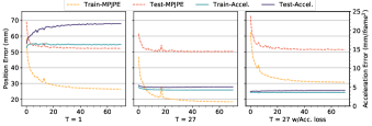
(a) 3D Skeleton-based Methods [29, 35]

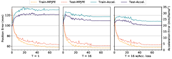
(b) SMPL-based Methods [21]

Figure 1: Comparison MPJPE and Accel during training and testing stages of single-frame ($T=1$) [29] and temporal ($T=27$ or $T=16$) [35, 21] pose estimation and mesh recovery methods. w/Acc. loss adds an acceleration loss in the training stage. In (b) T = 1, we simply remove GRUs and set sequence length as $1$.

2.1 Rethink Existing Spatio-temporal Models

To explore the bottleneck of existing methods using spatio-temporal models to optimize precision and smoothness concurrently, we perform experiments on popular 3D skeleton-based methods [29, 35] and SMPL-based methods [22, 21]. In terms of the single-frame approaches ($T=1$), we implement the simple baseline FCN [29] for 3D pose estimation tested on the Human3.6M dataset and remove GRUs in VIBE [21] for body recovery tested on the 3DPW dataset. For multi-frame methods ($T>1$), we apply the video-based 3D pose estimator VPose [35], conducting temporal convolution networks with dilated convolution along the time axis and the official VIBE [21]. The difference between single-frame methods and multi-frame methods is different from aggregation strategies along the temporal dimension. Two evaluation metrics, mean position errors (MPJPE) and acceleration errors (Accel) are used.

Figure 1 illustrates the training and testing performance for both MPJPE and Accel. For single-frame models ($T=1$) [29, 22], we observe that the position errors decrease, but the acceleration errors become larger as the epochs increase, indicating that the single-frame methods which extract only spatial information are likely to sacrifice smoothness in exchange for localization performance improvement. It is important to exploit temporal information explicitly.

For multi-frame approaches [35, 21] ($T=27$), they make use of temporal information by TCNs [35] and GRUs [21] respectively and improve both precision and smoothness. Yet, their loss function is applied to each frame, and their smoothness is still far from satisfactory, which is intuitively not beneficial for smoothness optimization.

Accordingly, to further improve smoothness as previous works did [19, 45], we add an acceleration (Acc.) loss on the per-frame L1 loss, which constrains the estimated acceleration to be as close as the ground truth’s acceleration. As shown in the right ones ($T=27$ w/ Acc. loss), although the acceleration errors decrease slightly, the position errors increase instead. It implies that it is hard to achieve optimal precision and smoothness simultaneously within existing frameworks (including models and loss functions). The reasons behind this may lie in that temporal and spatial information may generalize and overfit at different rates as two different modalities. MPJPEs are always larger than Accels, making the models pay more attention to optimizing spatial errors and hard to reduce Accels greatly. This observation motivates us to design the temporal-only refinement paradigm.

Moreover, to quantitatively explore the combination strategies of SmoothNet with existing backbones, whether training two models together (the one-stage strategy) or training them separately (the two-stage method), we try each of them on 3d pose estimation and body recovery. Specifically, if SmoothNet is trained together with the backbones in an end-to-end manner (w/ $B$), it belongs to the one-stage strategy. And if SmoothNet is trained separately, it is called the two-stage method. As presented in Table 2, we can find that (i) the spatio-temporal model [35] with multiple frames as inputs will gain in both Accel (smoothness) and MPJPE (precision), but the computational costs will be increased; (ii) adding acceleration loss or SmoothNet in an end-to-end way can benefit Accel but harm MPJPE; (iii) adding intermediate L1 supervision between the backbones and SmoothNet (w/ $B$ $\circ$) shows a slight drop in performance, but after adding an additional acceleration loss will improve both metrics. Compared with one-stage strategies, two-stage solutions with a refinement network show their strengths in boosting both smoothness and precision.

Table 1: Comparison results of the body recovery from VIBE [21] of different training strategies on 3DPW. $\times$ means acceleration loss added in the loss function. $B$ means to add SmoothNet behind the backbones trained in an end-to-end manner.

	Strategy	Accel	MPJPE	PA-MPJPE	MPJVE
Backbones	In = 1	32.69	84.54	57.94	102.05
	In = 16	23.21	83.03	56.77	99.76
	In = 16 $\times$	20.42	84.51	57.81	101.62
	In = 16 w/ $B$	21.65	86.56	59.93	105.08
Ours	In = 1 w/ ours	6.12	82.98	57.27	100.67
	In = 16 w/ ours	6.05	81.42	56.21	98.83

Table 2: Comparison of the 3D pose estimation results from VPose [35] of different training strategies on Human3.6M. $\times$ means acceleration loss added in the loss function. $B$ means to add SmoothNet behind the origin network trained in an end-to-end manner. $\circ$ adds an intermediate L1 supervision between the backbone and SmoothNet.

	Strategy	Accel	MPJPE	Params.
Backbones	In = 1	19.17	54.55	6.39M
	In = 27	5.07	50.13	8.61M
	In = 27 w/ $\times$	4.12	51.48	8.61M
	In = 27 w/ $B$	2.78	52.65	8.65M
	In = 27 w/ $B$ $\times$	2.87	52.18	8.65M
	In = 27 w/ $B$ $\circ$	5.46	51.06	8.65M
	In = 27 w/ $B$ $\circ$ $\times$	2.69	50.94	8.65M
Ours	In = 1 w/ ours	1.03	52.72	0.03M
	In = 27 w/ ours	0.88	50.04	0.03M

2.2 More Comparison with Filters

In main paper Sec. 5.2, we compare the performance with filters on human body recovery. We first visualize the qualitative results on a specific axis to demonstrate the effectiveness of SmoothNet.

Qualitative comparison. Figure 2 illustrates the output positions of VIBE, VIBE with several Gaussian filters (G.F.,) of different kernel sizes, VIBE with our method, and the ground truth. The filters can relieve jitter errors with the increase of kernel size but suffers from over-smoothness when the kernel size is larger than $65$, leading to worse position errors. Instead, with a learnable design and long-range temporal receptive fields, SmoothNet has the capability to learn the long-range noisy patterns and capture more reliable estimations (e.g., near the $70_{th}$ and $220_{th}$ frames) of inputs, making it can not only relieve jitters but also narrow down biased errors consistently.

Figure 2: Performance comparison between filters and SmoothNet on refining the estimated results of VIBE on AIST++ dataset.

Quantitative comparison on 2D and 3D pose estimation. We further show more results on the tasks of 2D pose estimation and 3D pose estimation on Human3.6M. In Table 3, the upper half table of each task compares the results of filters with the closest MPJPEs to ours, and the lower half table compares the performance of filters with the most similar Accel to ours. We can conclude that our approach achieves better performance on both precision and smoothness, validating that the temporal-only network with a long-range effective receptive field will be a good solution.

Table 3: Comparison of most used filters with different estimated poses from CPN [5] (2D) and FCN [29] (3D) on Human3.6M.

	Method	Accel	MPJPE	PA-MPJPE	Test FPS
2D Pose	CPN [5]	2.91	6.67	5.18	-
	w/One-Euro [4]	0.51	7.86	5.47	2.28k
	w/Savitzky-Golay [36]	0.20	6.52	4.99	67.39k
	w/Gaussian1d [46]	0.51	6.55	5.00	35.97k
	w/One-Euro [4]	0.19	9.21	6.01	3.93k
	w/Savitzky-Golay [36]	0.15	8.23	5.89	65.10k
	w/Gaussian1d [46]	0.14	6.73	4.99	43.74k
	w/Ours	0.14	6.45	4.96	71.60k
3D Pose	FCN [29]	19.17	54.55	42.20	-
	w/One-Euro [4]	3.80	55.20	42.73	2.27k
	w/Savitzky-Golay [36]	1.34	53.48	41.49	66.37k
	w/Gaussian1d [46]	2.43	53.67	41.60	29.54k
	w/One-Euro [4]	0.94	143.24	85.35	3.72k
	w/Savitzky-Golay [36]	0.92	74.38	57.25	65.56k
	w/Gaussian1d [46]	0.95	83.54	68.53	28.93k
	w/Ours	1.03	52.72	40.92	66.67k

2.3 Results of Additional Metrics

To explore the effect on significant errors and long-term jitters, we calculate the worst 1% of MPJPEs (MPJPE-1%) and the worst 1% Accel (Accel-1%) and the corresponding improvement by SmoothNet. The results of Humane3.6M is shown in the main paper. For the reason that significant errors and long-term jitters are usually accompanied by large estimation errors, as shown in Tab.  4 and Tab. 5, the improvement on MPJPE-1% and Accel-1% proves the smoothing ability of SmoothNeton long-term and large jitters.

Table 4: MPJPE-1% and Accel-1% improvement on 3D pose estimation. The results of Humane3.6M is shown in the main paper.

Improvement of MPJPE-1% and Accel-1% on 3D pose estimation
Dataset	AIST++			3DPW
Estimator	SPIN	TCMR	VIBE	EFT	PARE	SPIN	TCMR	VIBE
MPJPE-1%	352.93	373.18	339.56	278.51	225.72	289.89	249.11	257.83
MPJPE-1% w/ours	236.85	328.53	235.01	210.72	192.26	224.64	239.53	208.26
Accel-1%	195.48	43.94	177.07	218.71	132.82	199.33	43.81	123.92
Accel-1% w/ours	12.38	12.30	11.98	29.73	31.75	25.88	30.80	26.11
Dataset	MPI-INF-3DHP			MuPoTS
Estimator	SPIN	TCMR	VIBE	TposeNet		TposeNet w/RefineNet
MPJPE-1%	273.73	255.93	253.58	354.87		277.79
MPJPE-1% w/ours	241.62	246.64	238.57	347.36		265.98
Accel-1%	107.00	16.73	57.05	33.75		26.65
Accel-1% w/ours	9.89	9.24	9.11	6.17		8.75

Table 5: MPJPE-1% and Accel-1% improvement on SMPL pose estimation.

Improvement of MPJPE-1% and Accel-1% on SMPL Pose
Dataset	AIST++			3DPW
Estimator	SPIN	TCMR	VIBE	EFT	PARE	SPIN	TCMR	VIBE
MPJPE-1%	355.85	374.36	341.80	272.32	232.71	283.56	251.94	255.49
MPJPE-1% w/ours	270.94	352.54	274.19	223.91	207.05	236.66	249.34	218.57
Accel-1%	195.00	44.13	176.63	205.32	130.74	185.50	38.26	118.80
Accel-1% w/ours	19.97	24.51	23.19	42.32	31.96	33.18	36.39	31.28

2.4 Comparison with RefineNet

For learning-based jitter mitigation methods, we choose RefineNet [43] for comparison on the multi-person 3D pose estimation dataset MuPoTS-3D [32]. We compare them on the universal coordinates, where each person is rescaled according to the hip and has a normalized height. We also show the refinement results with two filters for comparison. As RefineNet [43] has compared with the interpolation methods and One-Euro filter [4] and showed better performance, we do not list their results here. To better fit the test set MuPoTS-3D, RefineNet is trained on two multi-person 3D poses datasets: MPI-INF-3DHP dataset [30] and an in-distribution MuCo-Temp dataset generated by the authors. In contrast, SmoothNet is trained on VIBE-AIST++ (the same model used in the previous experiment) without any finetuning to explore the generalization capability of SmoothNet across datasets.

Table 6: Comparison results on multi-person MuPoTS-3D dataset [32]. SmoothNet is directly tested on it, while RefineNet [43] has been trained on in-domain datasets.

Method	Accel	MPJPE	PA-MPJPE
TPoseNet [43]	12.70	103.33	68.36
TPoseNet w/ RefineNet [43]	9.53	93.97	65.16
TPoseNet w/ Savitzky-Golay	8.29	102.79	68.30
TPoseNet w/ Gaussian1d	8.61	102.70	68.17
TPoseNet w/ Ours	7.23	100.78	68.10
RefineNet w/ Savitzky-Golay	7.22	93.75	65.34
RefineNet w/ Gaussian1d	8.40	93.65	65.19
RefineNet w/ Ours	7.21	91.78	65.06

In Table 6, we first analyze the refinement results for the TPoseNet pose estimator [43], which is a temporal residual convolutional network for 2D-to-3D pose estimation used as the backbone network in RefineNet. Although the MPJPE of RefineNet drops the most as it has been trained on the relevant datasets, its Accel is the highest, indicating that the smoothing capability of RefineNet cannot outperform filter-based solutions [46, 36]. Our method further improves on Accel by $8.35$% compared to the best filter solution. At the same time, as a data-driven method, even though SmoothNet is trained on a different dataset, it shows a $1.9$% reduction in pose estimation errors compared to the motion-oblivious filter-based solutions.

Finally, it is possible to refine the pose outputs from RefineNet with filters and SmoothNet, and we show the results in the bottom half of Table 6. As observed from the table, all the methods result in performance improvement. Among them, SmoothNet again obtains the largest improvements, i.e., $24.3$% and $2.3$% in Accel and MPJPE, respectively. Such results demonstrate the effectiveness of the proposed solution on top of any learning-based pose estimators.

2.5 Generalization Ability

SmoothNetis a temporal-only network, which has good generalization ability across backbones, modalities, and datasets. By default, we provide three pretrained models (Trained 3D positions on the FCN estimator on Human3.6M, SPIN on 3DPW [28], and VIBE on AIST++ [25]), covering all existing cases and making Accels reduce greatly. Due to motion distribution shift, the results of MPJPEs and PA-MPJPEs will be influenced.

To explore the generalization ability, we present test results (shown in the left two columns) under the three pretrained models (shown in the third row) in Table 7,  8,  9. The background color highlights the increase and decrease degree SmoothNetoutputs have compared with inputs. The greener the background is, the better output result is. The redder the background is, the worse the output reulst is. We have some observations as follows. First, for all models, the Accels are lower than INPUT estimators by a large margin (illustrated as green background), indicating that they have similar smoothing capability. Second, for MPJPEs and PA-MPJPEs, we can find at least one model with better accuracy than results from INPUT estimators. Third, the MPJPEs will be lower if the trained datasets are the same or have similar distribution to the test datasets.

Table 7: Comparison results on generalization ability across modality (from 3d position to 6d rotation matrix) and backbones (shown in the left two columns) under the three pretrained SmoothNet(shown in the third row). Green background means great improvement, while red background highlights the worse results compared with Input estimators.

Generalization Ability on SMPL Pose Estimation
Mertrics		Accel				MPJPE				PA-MPJPE
Test Dataset	Train \ Test	INPUT	AIST++	H36M	3DPW	INPUT	AIST++	H36M	3DPW	INPUT	AIST++	H36M	3DPW
	SPIN	33.21	5.72	5.81	6.24	107.72	103.00	104.03	105.04	74.39	70.98	71.69	72.06
	TCMR	6.47	4.70	4.68	4.70	106.95	108.19	106.39	107.19	71.58	71.89	71.33	71.43
AIST++	VIBE	31.65	5.88	5.95	6.34	107.41	102.06	104.48	105.21	72.83	69.49	70.38	70.74
	EFT	33.38	7.67	7.71	7.89	91.6	91.79	90.54	89.57	55.33	54.96	55.25	54.40
	PARE	26.45	6.29	6.28	6.31	79.93	81.37	79.93	78.68	48.74	49.14	49.49	48.47
	SPIN	34.95	7.22	7.22	7.40	99.28	98.98	98.12	97.81	61.71	61.79	61.97	61.19
	TCMR	7.12	6.50	6.52	6.48	88.46	89.82	88.37	88.69	55.70	57.22	55.97	56.61
3DPW	VIBE	23.59	5.98	7.24	7.42	84.27	85.89	83.14	83.46	54.92	52.49	54.6	54.83

Table 8: Comparison results on generalization ability across modality (from 3d position to 2d position) and backbones (shown in the left two columns) under the three pretrained SmoothNet(shown in the third row).

Generalization Ability on 2D Pose Estimation
Mertrics		Accel				MPJPE				PA-MPJPE
Test Dataset	Train \ Test	INPUT	AIST++	H36M	3DPW	INPUT	AIST++	H36M	3DPW	INPUT	AIST++	H36M	3DPW
	CPN	2.91	0.16	0.14	0.17	6.67	8.52	6.45	8.09	5.18	5.88	4.96	5.44
	Hourglass	1.54	0.15	0.15	0.16	9.42	10.64	9.25	9.92	7.64	8.3	7.57	7.49
	HRNet	1.01	0.13	0.13	0.14	4.59	7.09	4.54	6.39	4.19	5.47	4.13	4.63
H36M	RLE	0.9	0.13	0.13	0.13	5.14	7.67	5.11	7.18	4.82	6.04	4.78	5.3

Table 9: Comparison results on generalization ability across backbone under the three pretrained SmoothNet(shown in the third row).

Generalization Ability on 3D Pose Estimation
Evaluation Mertrics		Accel				MPJPE				PA-MPJPE
Test Dataset	Train \ Test	INPUT	AIST	H36M	3DPW	INPUT	AIST	H36M	3DPW	INPUT	AIST	H36M	3DPW
	SPIN	33.19	4.17	4.23	4.54	107.17	95.21	104.03	100.91	74.40	69.98	72.71	72.20
	TCMR	6.40	4.24	4.23	4.21	106.72	105.51	105.84	105.99	71.59	72.23	71.61	71.90
AIST	VIBE	31.64	4.15	4.22	4.50	106.90	97.47	104.01	103.31	72.84	69.67	71.26	70.89
	FCN	19.17	1.07	1.03	1.20	54.55	61.79	52.72	58.22	42.20	43.85	40.92	41.87
	RLE	7.75	0.91	0.90	0.95	48.87	53.29	48.27	51.28	38.63	40.54	38.13	38.43
	TCMR	3.77	2.80	2.79	2.81	73.57	80.43	73.89	79.99	52.04	53.72	52.13	53.33
	VIBE	15.81	2.86	2.86	2.97	78.10	84.89	77.23	82.94	53.67	54.85	53.35	54.06
	VideoPose (T=243)	2.82	0.88	0.87	0.88	48.11	53.93	48.05	52.58	37.71	39.74	37.66	38.16
	VideoPose (T=27)	3.53	0.90	0.88	0.90	50.13	55.57	50.04	54.27	39.13	41.01	39.04	39.50
H36M	VideoPose (T=81)	3.06	0.88	0.87	0.89	48.97	54.64	48.89	53.26	38.27	40.27	38.21	38.74
	SPIN	28.54	6.42	6.41	6.54	100.74	94.35	101.76	92.89	61.35	62.9	62.51	60.22
	TCMR	7.92	6.47	6.45	6.49	92.83	91.45	93.79	88.93	58.16	60.57	59.21	58.89
MPI-INF -3DHP	VIBE	22.37	6.37	6.38	6.50	92.39	87.81	93.33	87.57	58.85	60.03	59.91	58.84
	TposeNet	12.70	7.23	7.23	7.29	103.33	100.78	102.08	101.21	68.36	68.10	67.80	68.38
MuPoTS	TposeNet w/ RefineNet	9.53	7.21	7.20	7.23	93.97	91.78	93.34	92.03	65.16	65.06	64.83	65.33
	EFT	29.03	5.30	5.30	5.44	81.60	79.79	80.57	79.48	48.78	49.08	48.91	48.54
	PARE	22.77	5.24	5.22	5.31	71.80	72.27	71.36	71.11	43.44	45.18	43.49	43.58
	SPIN	30.84	5.36	5.35	5.53	87.58	87.99	85.60	86.67	53.28	54.42	53.08	52.74
	TCMR	6.76	5.96	5.95	5.96	86.46	87.70	86.48	87.62	52.67	53.61	53.00	53.41
3DPW	VIBE	23.16	5.98	5.98	6.12	82.97	85.89	81.49	84.39	52.00	52.49	51.70	52.06

2.6 Smoothness on Synthetic Data

Due to the lack of pairwise labeled data, some approaches  [11] for Mocap sensors denoising verify the validity of their approaches on synthetic noise, like Gaussian noises. We follow their methods to generate the noisy poses, adding different levels of Gaussian noises on the ground truth data. We take the Human3.6M dataset as an example. In the training stage, we generate Gaussian noises with the probability $p$ and noise variance $\sigma$ on the ground truth 2D or 3D positions for 2D or 3D pose estimation respectively as synthetic training data. SmoothNet can be trained on these synthetic data. In the inference stage, we also add the same noise level to the testing set as the synthetic test data. Table 10 gives the corresponding results of our model. SmoothNet can refine the noises/jitters at a large margin without any spatial correlations since it utilizes the smoothness prior of human motions. For instance, in terms of 3D pose estimation, either as the variance of Gaussian noises increase from 10mm to 100mm or the probability changes from $0.1$ to $0.9$, SmoothNet can decrease Accel and MPJPE at a large margin. Those results indicate SmoothNet will be also beneficial to remove different synthetic noises.

Table 10: Comparison of the 3D pose with different synthetic noises from Gaussian Noise on Human3.6M. $p$ is the probability of adding noise, and $\sigma$ means the variance. pix. is the abbreviation of the pixel.

	Gaussion Noise	In Accel	Out Accel	In MPJPE	Out MPJPE
2D Pose	$p$ = 0.5, $\sigma$ = 10 pix.	10.10	0.20	3.56	0.83
	$p$ = 0.5, $\sigma$ = 50 pix.	50.53	0.35	17.80	2.02
	$p$ = 0.5, $\sigma$ = 100 pix.	101.06	0.31	35.59	1.42
	$p$ = 0.1, $\sigma$ = 50 pix.	14.31	0.19	3.90	0.67
	$p$ = 0.5, $\sigma$ = 50 pix.	50.53	0.35	17.80	2.02
	$p$ = 0.9, $\sigma$ = 50 pix.	72.26	0.57	28.97	6.00
3D Pose	$p$ = 0.5, $\sigma$ = 10mm	26.25	0.84	9.68	3.54
	$p$ = 0.5, $\sigma$ = 50mm	131.25	1.55	48.42	7.00
	$p$ = 0.5, $\sigma$ = 100mm	262.49	1.24	96.84	20.38
	$p$ = 0.1, $\sigma$ = 50mm	40.68	1.03	11.46	2.46
	$p$ = 0.5, $\sigma$ = 50mm	131.25	1.55	48.42	7.00
	$p$ = 0.9, $\sigma$ = 50mm	184.32	2.10	74.46	16.85

2.7 More Ablation Study

Impact on Loss Function. As mentioned in the main paper Sec 4.3, we use $L_{pose}$+$L_{acc}$ as our final objective function. Here we explore how the loss functions affect the performance in Table 11. First, we find that only single-frame supervision $L_{pose}$ would be slightly worse than our result by $5.51$% in Accel, while the MPJPEs are competitive. It shows the precision can be optimized well by the $L_{pose}$. Next, only with $L_{acc}$ will make all results worst, indicating the significant necessity of $L_{pose}$ supervision. Last, adding $L_{pose}$ and $L_{acc}$ together to train the SmoothNet will benefit both smoothness and precision, proving that $L_{acc}$ companies with $L_{pose}$ can play its smooth role.

Table 11: Comparison of refined results by different loss functions based on the outputs of the SMPL-based method EFT [16] on the 3DPW dataset.

Method	Accel	MPJPE	PA-MPJPE
EFT	32.71	90.32	52.19
$L_{pose}$	6.42	86.63	50.82
$L_{acc}$	7.63	446.54	356.61
$L_{pose}$+$L_{acc}$	6.30	86.39	50.60

Impact on Motion Modalities. Motivated by this natural smoothness characteristic, we can unify various continuous modalities and make SmoothNet generalize well across them. In particular, 2D, 3D positions, and 6D rotation matrices are continuous modalities of the same space in neural networks. In contrast, the rotation representations as axis-angle or quaternion are discontinuous in the real Euclidean spaces [54], which may be hard for neural networks to learn. Accordingly, we explore the effects of these modalities used to train SmoothNet on EFT [16]. Table 12 shows the training results on each motion modality. We can see that the axis-angle or quaternion obtains worse results on both smoothness and precision. They may encounter some sudden changes/flips leading to poor results due to the discontinuity of the expression. Instead, the 6D rotation matrix and 3D position will be more suitable to learn and improve all metrics. Furthermore, 3D positions reach the best performance by decreasing $82.15$% in Accel, $5.72$% in MPJPE, and $3.60$% in PA-MPJPE.

Table 12: Comparison of refined results trained by different motion modalities based on the outputs of EFT [16] on the 3DPW dataset.

Method	Accel	MPJPE	PA-MPJPE
EFT [16]	32.71	90.32	52.19
Angle-Axis	77.89	172.17	51.38
Quaternion	28.50	91.23	51.03
6D Rotation	6.43	86.92	50.87
3D Position	6.30	86.39	50.60

Last, to explore whether there is also better generalization between different continuous modalities, such as 3D position and 6D rotation matrix, cross-modality tests were carried out demonstrated in Table 13. We can summarize these observations: (i) when tested across modalities, all results will be worse relative to the modality the model trained on; (ii) SmoothNet trained in 3D positions, smoothed directly over the representation of the 6D rotation matrix, can achieve even better performance than training on the 6D rotation matrix itself. Hence, these results motivate us to use 3D positions as supervision by default, where 3D positions contain more information than 2D positions, and their ground-truth are usually more precise than the 6D rotation matrix (explicitly found in the AIST++ dataset, like Figure 3).

Table 13: Comparison of refined results by cross motion representations testing based on the outputs of EFT [16] on the 3DPW dataset. Cross-Test means training the SmoothNet on a motion representation while testing it on another modality directly.

Method	Accel	MPJPE	PA-MPJPE
EFT	32.71	90.32	52.19
6D Rotation	6.43	86.92	50.87
Cross-Test on 3D Position	7.10	88.13	51.79
3D Position	6.30	86.39	50.60
Cross-Test on 6D Rotation	6.47	86.82	50.81

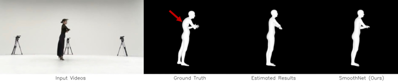
Figure 3: Comparison the results of the ground truth, VIBE [21] with VIBE w/ SmoothNet on AIST++ dataset.

Effect of Normalization Strategies. Normalization is an effective way to calibrate biased errors and improve the generalization ability. As a plug-and-play network, we also explore how different normalization strategies influence the results, especially the generalization ability. In the main paper, we do not use any normalization by default.

We adopt three normalization strategies. Particularly, w/o Norm. denotes taking the original estimated results without normalization. Sequence Norm. indicates normalizing each input axis $\mathbf{\hat{Y}}_{i}$ with means and variances computed from input sequences along the axis. Because the estimated inputs are always noisy and the bias shift between the training data and testing data, the above normalization methods will be affected. Instead, using the mean and variance from the ground truth (with $\dagger$) along each axis can avoid such influences and we can explore the upper bound performance under the Sequence Norm. normalization.

Table 14: Comparison of the results of different normalization based on the outputs of EFT [16] and cross-backbone testing on the outputs of TCMR [6] on 3DPW dataset. $\dagger$ means using the same mean and variance as the ground truth to explore the upper bound performance.

Method	Accel	MPJPE	PA-MPJPE
EFT [16]	32.71	90.32	52.19
w/o Norm.	5.80	85.16	50.31
Sequence Norm.	5.82	88.21	51.06
Sequence Norm. $\dagger$	5.80	61.65	44.28
TCMR [6]	6.76	86.46	52.67
w/o Norm.	5.91	86.04	52.42
Sequence Norm	6.00	86.34	52.87
Sequence Norm $\dagger$	5.92	68.51	49.15

In Table 14, we compare the performance of different normalizations based on the outputs of EFT [16] on the 3DPW dataset in the upper table. We can discover that the smoothing ability for all normalizations is similar, and the main difference lies in the degree of biased error removal. To be specific, under the Sequence Norm. $\dagger$ normalization, the MPJPE can decrease from $85.16$mm to $61.65$mm, improved by $27.5$%. To explore the generalization ability across backbones, we further test SmoothNet trained on EFT-3DPW on TCMR [6]-3DPW. From the lower part of the table, we can get similar conclusions as above. In specific, SmoothNet can reduce Accel from $6.77mm/frame^{2}$ to about $6mm/frame^{2}$, and the upper bound of MPJPE can be $68.51mm$ (improvement by $20.8$%) from the refinement stage.

3 Qualitative Results

As jitters seriously affect visual effect, we visualize the results from several tasks, such as 2D pose estimation, 3D pose estimation, and model-based body recovery. For 2D and 3D pose estimation, we show two kinds of actions on Human3.6M respectively with the corresponding Accel and MPJPE for each frame. The estimated 2D poses are from the single-frame SOTA method RLE [24], and the estimated 3D poses are from the single-frame method FCN [29]. For model-based methods, the estimated results come from VIBE [21] on AIST++ dataset and SPIN [22] on 3DPW dataset.

We can observe that the jitters in a video are highly-unbalanced, where most frames suffer from slight jitters while long-term significant jitters will be accompanied by large biased errors. SmoothNet can relieve not only small jitters but long-term jitters well. And it can boost both smoothness and precision significantly. Specifically, unlike low-pass filters [11, 36, 13], our method can estimate the high-frequency movements well, like the action Posing. Finally, we observe that the ground-truth 6D rotation matrices from AIST++ is not quite accurate, as the SMPL annotations are fitted with few constraints. For example, the red arrow in Figure 3 illustrates that a SMPL fitting from AIST++ has a bulging back problem. Instead, their $14$ skeletal 3D positions are more precise. When it comes to model training, the quality of annotation is crucial for the success of a data-driven model. As SmoothNet is devised to operate on temporal axis, it is capable of training on one modality and testing on the other, so as to have the flexibility of choosing more precise annotated modality for training. This property makes SmoothNet applicable to datasets with different annotation qualities from different modalities.

References

- [1] Andriluka, M., Pishchulin, L., Gehler, P., Schiele, B.: 2d human pose estimation: New benchmark and state of the art analysis. In: Proceedings of the IEEE Conference on computer Vision and Pattern Recognition. pp. 3686–3693 (2014)
- [2] Bai, S., Kolter, J.Z., Koltun, V.: An empirical evaluation of generic convolutional and recurrent networks for sequence modeling. ArXiv abs/1803.01271 (2018)
- [3] Brownrigg, D.R.: The weighted median filter. Communications of the ACM 27(8), 807–818 (1984)
- [4] Casiez, G., Roussel, N., Vogel, D.: 1€ filter: a simple speed-based low-pass filter for noisy input in interactive systems. In: Proceedings of the SIGCHI Conference on Human Factors in Computing Systems. pp. 2527–2530 (2012)
- [5] Chen, Y., Wang, Z., Peng, Y., Zhang, Z., Yu, G., Sun, J.: Cascaded pyramid network for multi-person pose estimation. In: Proceedings of the IEEE Conference on Computer Vision and Pattern Recognition. pp. 7103–7112 (2018)
- [6] Choi, H., Moon, G., Chang, J.Y., Lee, K.M.: Beyond static features for temporally consistent 3d human pose and shape from a video. In: Proceedings of the IEEE/CVF Conference on Computer Vision and Pattern Recognition. pp. 1964–1973 (2021)
- [7] Choutas, V., Pavlakos, G., Bolkart, T., Tzionas, D., Black, M.J.: Monocular expressive body regression through body-driven attention. In: European Conference on Computer Vision. pp. 20–40. Springer (2020)
- [8] Coskun, H., Achilles, F., DiPietro, R.S., Navab, N., Tombari, F.: Long short-term memory kalman filters: Recurrent neural estimators for pose regularization. 2017 IEEE International Conference on Computer Vision (ICCV) pp. 5525–5533 (2017)
- [9] Dosovitskiy, A., Beyer, L., Kolesnikov, A., Weissenborn, D., Zhai, X., Unterthiner, T., Dehghani, M., Minderer, M., Heigold, G., Gelly, S., et al.: An image is worth 16x16 words: Transformers for image recognition at scale. arXiv preprint arXiv:2010.11929 (2020)
- [10] Fischman, M.G.: Programming time as a function of number of movement parts and changes in movement direction. Journal of Motor Behavior 16(4), 405–423 (1984)
- [11] Gauss, J.F., Brandin, C., Heberle, A., Löwe, W.: Smoothing skeleton avatar visualizations using signal processing technology. SN Computer Science 2(6), 1–17 (2021)
- [12] Hunter, J.S.: The exponentially weighted moving average. Journal of quality technology 18(4), 203–210 (1986)
- [13] Hyndman, R.J.: Moving averages. (2011)
- [14] Ionescu, C., Papava, D., Olaru, V., Sminchisescu, C.: Human3. 6m: Large scale datasets and predictive methods for 3d human sensing in natural environments. IEEE transactions on pattern analysis and machine intelligence 36(7), 1325–1339 (2013)
- [15] Jiang, T., Camgoz, N.C., Bowden, R.: Skeletor: Skeletal transformers for robust body-pose estimation. In: Proceedings of the IEEE/CVF Conference on Computer Vision and Pattern Recognition. pp. 3394–3402 (2021)
- [16] Joo, H., Neverova, N., Vedaldi, A.: Exemplar fine-tuning for 3d human model fitting towards in-the-wild 3d human pose estimation. In: 2021 International Conference on 3D Vision (3DV). pp. 42–52. IEEE (2021)
- [17] Kalman, R.E.: A new approach to linear filtering and prediction problems (1960)
- [18] Kanazawa, A., Black, M.J., Jacobs, D.W., Malik, J.: End-to-end recovery of human shape and pose. In: Proceedings of the IEEE conference on computer vision and pattern recognition. pp. 7122–7131 (2018)
- [19] Kanazawa, A., Zhang, J.Y., Felsen, P., Malik, J.: Learning 3d human dynamics from video. In: Proceedings of the IEEE/CVF Conference on Computer Vision and Pattern Recognition. pp. 5614–5623 (2019)
- [20] Kim, D.Y., Chang, J.Y.: Attention-based 3d human pose sequence refinement network. Sensors 21(13), 4572 (2021)
- [21] Kocabas, M., Athanasiou, N., Black, M.J.: Vibe: Video inference for human body pose and shape estimation. In: Proceedings of the IEEE/CVF Conference on Computer Vision and Pattern Recognition. pp. 5253–5263 (2020)
- [22] Kolotouros, N., Pavlakos, G., Black, M.J., Daniilidis, K.: Learning to reconstruct 3d human pose and shape via model-fitting in the loop. In: Proceedings of the IEEE/CVF International Conference on Computer Vision. pp. 2252–2261 (2019)
- [23] Lee, C.H., Lin, C.R., Chen, M.S.: Sliding-window filtering: an efficient algorithm for incremental mining. In: Proceedings of the tenth international conference on Information and knowledge management. pp. 263–270 (2001)
- [24] Li, J., Bian, S., Zeng, A., Wang, C., Pang, B., Liu, W., Lu, C.: Human pose regression with residual log-likelihood estimation. In: ICCV (2021)
- [25] Li, R., Yang, S., Ross, D.A., Kanazawa, A.: Ai choreographer: Music conditioned 3d dance generation with aist++. In: Proceedings of the IEEE/CVF International Conference on Computer Vision (ICCV). pp. 13401–13412 (October 2021)
- [26] Lin, T.Y., Maire, M., Belongie, S., Hays, J., Perona, P., Ramanan, D., Dollár, P., Zitnick, C.L.: Microsoft coco: Common objects in context. In: European conference on computer vision. pp. 740–755. Springer (2014)
- [27] Luo, Z., Golestaneh, S.A., Kitani, K.M.: 3d human motion estimation via motion compression and refinement. In: Proceedings of the Asian Conference on Computer Vision (2020)
- [28] von Marcard, T., Henschel, R., Black, M.J., Rosenhahn, B., Pons-Moll, G.: Recovering accurate 3d human pose in the wild using imus and a moving camera. In: Proceedings of the European Conference on Computer Vision (ECCV). pp. 601–617 (2018)
- [29] Martinez, J., Hossain, R., Romero, J., Little, J.J.: A simple yet effective baseline for 3d human pose estimation. In: Proceedings of the IEEE International Conference on Computer Vision. pp. 2640–2649 (2017)
- [30] Mehta, D., Rhodin, H., Casas, D., Fua, P., Sotnychenko, O., Xu, W., Theobalt, C.: Monocular 3d human pose estimation in the wild using improved cnn supervision. In: 2017 international conference on 3D vision (3DV). pp. 506–516. IEEE (2017)
- [31] Mehta, D., Sotnychenko, O., Mueller, F., Xu, W., Elgharib, M., Fua, P., Seidel, H.P., Rhodin, H., Pons-Moll, G., Theobalt, C.: Xnect: Real-time multi-person 3d motion capture with a single rgb camera. ACM Transactions on Graphics (TOG) 39(4), 82–1 (2020)
- [32] Mehta, D., Sotnychenko, O., Mueller, F., Xu, W., Sridhar, S., Pons-Moll, G., Theobalt, C.: Single-shot multi-person 3d pose estimation from monocular rgb. 2018 International Conference on 3D Vision (3DV) pp. 120–130 (2018)
- [33] Mehta, D., Sridhar, S., Sotnychenko, O., Rhodin, H., Shafiei, M., Seidel, H.P., Xu, W., Casas, D., Theobalt, C.: Vnect: Real-time 3d human pose estimation with a single rgb camera. ACM Transactions on Graphics (TOG) 36(4), 1–14 (2017)
- [34] Newell, A., Yang, K., Deng, J.: Stacked hourglass networks for human pose estimation. In: European conference on computer vision. pp. 483–499. Springer (2016)
- [35] Pavllo, D., Feichtenhofer, C., Grangier, D., Auli, M.: 3d human pose estimation in video with temporal convolutions and semi-supervised training. In: Proceedings of the IEEE Conference on Computer Vision and Pattern Recognition. pp. 7753–7762 (2019)
- [36] Press, W.H., Teukolsky, S.A.: Savitzky-golay smoothing filters. Computers in Physics 4(6), 669–672 (1990)
- [37] So, D., Le, Q., Liang, C.: The evolved transformer. In: International Conference on Machine Learning. pp. 5877–5886. PMLR (2019)
- [38] Sun, K., Xiao, B., Liu, D., Wang, J.: Deep high-resolution representation learning for human pose estimation. In: Proceedings of the IEEE/CVF Conference on Computer Vision and Pattern Recognition. pp. 5693–5703 (2019)
- [39] Tripathi, S., Ranade, S., Tyagi, A., Agrawal, A.: Posenet3d: Learning temporally consistent 3d human pose via knowledge distillation. In: 2020 International Conference on 3D Vision (3DV). pp. 311–321. IEEE (2020)
- [40] Tsuchida, S., Fukayama, S., Hamasaki, M., Goto, M.: Aist dance video database: Multi-genre, multi-dancer, and multi-camera database for dance information processing. In: ISMIR. pp. 501–510 (2019)
- [41] Van Loan, C.: Computational frameworks for the fast Fourier transform. SIAM (1992)
- [42] Vaswani, A., Shazeer, N., Parmar, N., Uszkoreit, J., Jones, L., Gomez, A.N., Kaiser, Ł., Polosukhin, I.: Attention is all you need. Advances in neural information processing systems 30 (2017)
- [43] Véges, M., Lőrincz, A.: Temporal smoothing for 3d human pose estimation and localization for occluded people. In: International Conference on Neural Information Processing. pp. 557–568. Springer (2020)
- [44] Wan, Z., Li, Z., Tian, M., Liu, J., Yi, S., Li, H.: Encoder-decoder with multi-level attention for 3d human shape and pose estimation. In: Proceedings of the IEEE/CVF International Conference on Computer Vision. pp. 13033–13042 (2021)
- [45] Wang, J., Yan, S., Xiong, Y., Lin, D.: Motion guided 3d pose estimation from videos. ArXiv abs/2004.13985 (2020)
- [46] Young, I.T., Van Vliet, L.J.: Recursive implementation of the gaussian filter. Signal processing 44(2), 139–151 (1995)
- [47] Zeng, A., Sun, X., Huang, F., Liu, M., Xu, Q., Lin, S.C.F.: Srnet: Improving generalization in 3d human pose estimation with a split-and-recombine approach. In: ECCV (2020)
- [48] Zeng, A., Sun, X., Yang, L., Zhao, N., Liu, M., Xu, Q.: Learning skeletal graph neural networks for hard 3d pose estimation. In: Proceedings of the IEEE International Conference on Computer Vision (2021)
- [49] Zhang, S., Zhang, Y., Bogo, F., Pollefeys, M., Tang, S.: Learning motion priors for 4d human body capture in 3d scenes. In: Proceedings of the IEEE/CVF International Conference on Computer Vision. pp. 11343–11353 (2021)
- [50] Zhao, L., Peng, X., Tian, Y., Kapadia, M., Metaxas, D.N.: Semantic graph convolutional networks for 3d human pose regression. In: Proceedings of the IEEE Conference on Computer Vision and Pattern Recognition. pp. 3425–3435 (2019)
- [51] Zheng, C., Zhu, S., Mendieta, M., Yang, T., Chen, C., Ding, Z.: 3d human pose estimation with spatial and temporal transformers. arXiv preprint arXiv:2103.10455 (2021)
- [52] Zhou, H., Zhang, S., Peng, J., Zhang, S., Li, J., Xiong, H., Zhang, W.: Informer: Beyond efficient transformer for long sequence time-series forecasting. In: Proceedings of AAAI (2021)
- [53] Zhou, K., Bhatnagar, B.L., Lenssen, J.E., Pons-Moll, G.: Toch: Spatio-temporal object correspondence to hand for motion refinement. In: arXiv (May 2022)
- [54] Zhou, Y., Barnes, C., Lu, J., Yang, J., Li, H.: On the continuity of rotation representations in neural networks. 2019 IEEE/CVF Conference on Computer Vision and Pattern Recognition (CVPR) pp. 5738–5746 (2019)