Robust approximation of generalized Biot-Brinkman problems

Abstract

The generalized Biot-Brinkman equations describe the displacement, pressures and fluxes in an elastic medium permeated by multiple viscous fluid networks and can be used to study complex poromechanical interactions in geophysics, biophysics and other engineering sciences. These equations extend on the Biot and multiple-network poroelasticity equations on the one hand and Brinkman flow models on the other hand, and as such embody a range of singular perturbation problems in realistic parameter regimes. In this paper, we introduce, theoretically analyze and numerically investigate a class of three-field finite element formulations of the generalized Biot-Brinkman equations. By introducing appropriate norms, we demonstrate that the proposed finite element discretization, as well as an associated preconditioning strategy, is robust with respect to the relevant parameter regimes. The theoretical analysis is complemented by numerical examples.

1 Introduction

The study of the mechanical response of fluid-filled porous media – poromechanics – is essential in geophysics, biophysics and civil engineering. Through a series of seminal works dating from 1941 and onwards [7, 8], Biot introduced governing equations for the dynamic behavior of a linearly elastic solid matrix permeated by a viscous fluid with flow through the pore network described by Darcy’s law [17, 47]. Double-porosity models, extending upon Biot’s single fluid network to the case of two interacting networks, were used to describe the motion of liquids in fissured rocks as early as in the 1960s [5, 48, 32]. Later, multiple-network poroelasticity equations emerged in the context of reservoir modelling [4] to describe elastic media permeated by multiple networks characterised by different porosities, permeabilities and/or interactions. Since the early 2000s, poromechanics has been applied to model the heart [38, 13] as well as the brain and central nervous system [45, 44, 46, 16, 20].

In addition to interactions between fluid networks, recently also the viscous forces acting within each network have come to the fore [6, 14, 12, 31]. At its core, the effect of viscosity can be accounted for by replacing the Darcy approximation in the poroelasticity model by a Brinkman approximation [11, 40]. We here introduce multiple-network poroelasticity models incorporating viscosity under the term generalized Biot-Brinkman equations. In a bounded domain $\Omega\subset\mathbb{R}^{d}$, $d=1,2,3$ comprising $n$ fluid networks, the generalized Biot-Brinkman equations read as follows: find the displacement $\bm{u}=\bm{u}(x,t)$, fluid fluxes $\bm{v}_{i}=\bm{v}_{i}(x,t)$ and corresponding (negative) fluid pressures $p_{i}=p_{i}(x,t)$, for $i=1,\dots,n$ satisfying

(1a) $$-\operatorname{\mathrm{div}}\left(\bm{\sigma}(\bm{u})+\bm{\alpha}\cdot\bm{p}\bm{I}\right) =\bm{f},$$

(1b) $$-\nu_{i}\operatorname{\mathrm{div}}\bm{\varepsilon}(\bm{v}_{i})+\bm{v}_{i}-K_{i}\nabla p_{i} =\bm{r}_{i},$$

(1c) $$-c_{i}\dot{p}_{i}-\bar{\beta}_{i}p_{i}+\alpha_{i}\operatorname{\mathrm{div}}\dot{\bm{u}}+\operatorname{\mathrm{div}}\bm{v}_{i}+\bm{\beta}_{i}\cdot\bm{p} =g_{i},$$

over $\Omega\times(0,T)$ for $T>0$, and where (1b) and (1c) hold for $i=1,\ldots,n$. In (1a), we have introduced the vector notation $\bm{p}=(p_{1},\dots,p_{n})$ and $\bm{\alpha}=(\alpha_{1},\dots,\alpha_{n})$, where $\alpha_{i}$ is the Biot-Willis coefficient associated with network $i$. The elastic stress and strain tensors are:

(2) $$\bm{\sigma}(\bm{u})=2\mu\bm{\varepsilon}(\bm{u})+\lambda\text{div}(\bm{u})\bm{I},\quad\bm{\varepsilon}(\bm{u})=\frac{1}{2}(\nabla\bm{u}+(\nabla\bm{u})^{T}),$$

respectively, and with Lamé parameters $\mu$ and $\lambda$. Moreover, for each fluid network $i$, $\nu_{i}$ denotes the fluid viscosity and $K_{i}$ is its hydraulic conductance tensor. Furthermore, (1c) is an equivalent formulation of the standard multiple-network poroelasticity mass balance equations [4, 36, 24] with transfer coefficients $\beta_{ij}$, denoting $\bm{\beta}_{i}=(\beta_{i1},\dots,\beta_{in})$ and $\bar{\beta}_{i}=\sum_{j}\beta_{ij}$, when the fluid transfer into network $i$ is given by

$$\textstyle\sum_{j=1,j\not=i}^{n}\beta_{ij}(p_{i}-p_{j}).$$

The constants $c_{i}$ in (1c) denote the constrained specific storage coefficients, see e.g. [43] and the references therein. Finally, the prescribed right hand side $\bm{f}$ denotes body forces, while $g_{i}$ denotes a fluid source and $\bm{r}_{i}$ represents an external flux, both of the two latter in each network $i$. In the case $n=1$ and $\nu=0$, (1) reduces to the Biot equations.

The generalized Biot-Brinkman problem (1) defines a challenging system of PDEs to solve numerically. One reason for this is the large number of material parameters, several of which give rise to singular perturbation problems such as in the extreme cases of (near) incompressibility ($\lambda\rightarrow\infty$) and impermeability ($K_{i}\rightarrow 0$). Specifically, $\lambda\gg\mu$ is associated with numerical locking; if (1) is scaled by $1/\lambda$, the elastic term of the equation reads $\operatorname{\mathrm{div}}\frac{2\mu}{\lambda}\bm{\varepsilon}(\bm{u})+\nabla\operatorname{\mathrm{div}}\bm{u}=f$ which transforms from an $H^{1}$ problem to an $H(\operatorname{\mathrm{div}})$ problem as $\lambda$ tends to infinity. Similar singular perturbation problems arise, now for the flux variable $\bm{v}_{i}$, as $\nu_{i}$ tends to zero. Furthermore, certain parameter ranges of the storage coefficients and permeabilities ($K_{i}\ll c_{i})$ give rise to singular perturbation problems in the Darcy sub-system, see e.g. [37] and references therein. Finally, we mention that large transfer coefficients $\beta_{ij}$ and/or small Biot-Willis coefficients $\alpha_{i}$ can lead to strong coupling of the different subsystems and prevent direct exploitation of each subsystem’s properties.

In the case of vanishing viscosities ($\nu_{i}=0,\forall i$) the system (1) reduces to the multiple-network poroelasticity (MPET) equations. Robust and conservative numerical approximations of the MPET equations have been studied in the context of (near) incompressibility [36] as well as other material parameters [24, 27, 26]. Parameter-independent preconditioning and splitting schemes as well as a-posteriori error analysis and adaptivity have also been identified for the MPET equations [25, 27, 39, 18]. However, the generalized Biot-Brinkman system has received little attention from the numerical community. Therefore, the purpose of this paper is to identify and analyze stable finite element approximation schemes and preconditioning techniques for the time-discrete generalized Biot-Brinkman systems, with particular focus on parameter robustness.

This paper is organized as follows. After introducing notation, context and preliminaries in Section 2, we prove that the time-discrete generalized Biot-Brinkman system is well-posed in appropriate function spaces in Section 3. We introduce a fully discrete generalized Biot-Brinkman problem in Section 4 and prove that the discrete approximations satisfy a near optimal a-priori error estimate in appropriate norms independently of material parameters. We also propose a natural preconditioner. The theoretical analysis is complemented by numerical experiments in Section 5.

2 Preliminaries and notation

In this section of preliminaries, we give assumptions on the material parameters, present a rescaling of a time-discrete generalized Biot-Brinkman system and introduce parameter-weighted norms and function spaces.

2.1 Material parameters

We assume that the elastic Lamé coefficients satisfy the standard conditions $\mu>0$ and $d\lambda+2\mu>0$. The transfer coefficients are such that $\beta_{ij}=\beta_{ji}\geq 0$ for $i\not=j$ while $\beta_{ii}=0$, and the specific storage coefficients $c_{i}\geq 0$ for $i=1,\dots,n$. The Biot-Willis coefficients are bounded between zero and one by construction: $0<\alpha_{i}\leq 1$. We also assume that the hydraulic conductances $K_{i}>0$ for $i=1,\dots,n$. Further, our focus will be on the case $\nu_{i}>0$. For spatially-varying material parameters, we assume that each of the above conditions holds point-wise and that each parameter field is uniformly bounded from above and below.

2.2 Time discretization, rescaling and structure

Taking an implicit Euler time-discretization of (1) with uniform timestep $\tau$, multiplying (1c) by $\tau$, rearranging terms and removing the time-dependence from the notation, we obtain the following problem structure to be solved over $\Omega$ at each time step: find the unknown displacement $\bm{u}=\bm{u}(x)$, fluid fluxes $\bm{v}_{i}=\bm{v}_{i}(x)$ and corresponding (negative) fluid pressures $p_{i}=p_{i}(x)$, for $i=1,\dots,n$ satisfying

$$-\operatorname{\mathrm{div}}\left(\bm{\sigma}(\bm{u})+\bm{\alpha}\cdot\bm{p}\bm{I}\right) =\bm{f},$$

$$-\nu_{i}\operatorname{\mathrm{div}}\bm{\varepsilon}(\bm{v}_{i})+\bm{v}_{i}-K_{i}\nabla p_{i} =\bm{r}_{i},$$

$$-\left(c_{i}+\tau\bar{\beta}_{i}\right)p_{i}+\alpha_{i}\operatorname{\mathrm{div}}\bm{u}+\tau\operatorname{\mathrm{div}}\bm{v}_{i}+\tau\bm{\beta}_{i}\cdot\bm{p} =\tau g_{i}.$$

Multiplying by $\tau K_{i}^{-1}$ in the second equation(s) for the sake of symmetry gives

(4a) $$-\operatorname{\mathrm{div}}\left(\bm{\sigma}(\bm{u})+\bm{\alpha}\cdot\bm{p}\bm{I}\right) =\bm{f},$$

(4b) $$-\nu_{i}\tau K_{i}^{-1}\operatorname{\mathrm{div}}\bm{\varepsilon}(\bm{v}_{i})+\tau K_{i}^{-1}\bm{v}_{i}-\tau\nabla p_{i} =\tau K_{i}^{-1}\bm{r}_{i},$$

(4c) $$-\left(c_{i}+\tau\bar{\beta}_{i}\right)p_{i}+\alpha_{i}\operatorname{\mathrm{div}}\bm{u}+\tau\operatorname{\mathrm{div}}\bm{v}_{i}+\tau\bm{\beta}_{i}\cdot\bm{p} =\tau g_{i}.$$

For the sake of readability, we define

(5) $$s_{i}:=c_{i}+\tau\bar{\beta}_{i},\quad\gamma_{i}:=\tau\nu_{i}K_{i}^{-1}$$

recalling that $\bar{\beta}_{i}=\sum_{j}\beta_{ij}$ and $\beta_{ii}=0$, and set

(6) $$R^{-1}:=\max\{(1+\nu_{1})\tau K_{1}^{-1},\dots,(1+\nu_{n})\tau K_{n}^{-1}\}.$$

Using this notation, we introduce four $n\times n$ parameter matrices

(7) $$\Lambda_{1}=-\tau\begin{pmatrix}0&\beta_{12}&\dots&\beta_{1n}\\ \beta_{21}&0&\dots&\beta_{2n}\\ \vdots&\vdots&\ddots&\vdots\\ \beta_{n1}&\beta_{n2}&\dots&0\end{pmatrix}\\$$

and

(8) $$\Lambda_{2}=\operatorname{diag}(s_{1},s_{2},\dots,s_{n}),\quad\Lambda_{3}=\tau^{2}RI,\quad\Lambda_{4}=\frac{1}{2\mu+\lambda}\bm{\alpha}\bm{\alpha}^{T},$$

before defining

(9) $$\Lambda=\sum_{i=1}^{4}\Lambda_{i}.$$

In the case $n=1$, dropping the subscripts $i,j$ for readability and with the newly introduced parameter notation, the operator structure of the rescaled system (4) is

(10) $$\begin{pmatrix}-\operatorname{\mathrm{div}}\bm{\sigma}&\bm{0}&-\alpha\nabla\\ \bm{0}&-\gamma\operatorname{\mathrm{div}}\bm{\varepsilon}+\tau K^{-1}\bm{I}&-\tau\nabla\\ \alpha\operatorname{\mathrm{div}}&\tau\operatorname{\mathrm{div}}&-(\Lambda_{1}+\Lambda_{2})\\ \end{pmatrix}\begin{pmatrix}\bm{u}\\ \bm{v}\\ \bm{p}\end{pmatrix}=\begin{pmatrix}\bm{f}\\ \bm{r}\\ \bm{g}\end{pmatrix}$$

for $-(\Lambda_{1}+\Lambda_{2})=c\bm{I}$, and $\bm{p}=p$ in the $n=1$ case. The same structure holds for $n>2$ when denoting $\bm{v}^{T}=(\bm{v}_{1}^{T},\bm{v}_{2}^{T},\dots,\bm{v}_{n}^{T})$, $({\rm Div}\bm{v})^{T}=(\operatorname{\mathrm{div}}\bm{v}_{1},\dots,\operatorname{\mathrm{div}}\bm{v}_{n})$.

By the assumption of symmetric transfer, i.e. $\beta_{ij}=\beta_{ji}$, $\Lambda_{1}$ and $\Lambda$ are symmetric. Moreover, as $\Lambda_{1}+\Lambda_{2}$ is weakly diagonally dominant and thus symmetric positive semi-definite, $\Lambda_{3}$ is symmetric positive definite, and $\Lambda_{4}$ is symmetric positive semi-definite, it follows that $\Lambda$ is symmetric positive definite.

2.3 Domain and boundary conditions

Assume that $\Omega$ is open and bounded in $\mathbb{R}^{d}$, $d=2,3$ with Lipschitz boundary $\partial\Omega$. We consider the following idealized boundary conditions for the theoretical analysis of the time-discrete generalized Biot-Brinkman system (10) over $\Omega$. We assume that the displacement is prescribed (and equal to zero for simplicity) on the entire boundary $\partial\Omega$. Furthermore for each of the flux momentum equations we assume datum on the normal flux $\bm{v}_{i}\cdot\bm{n}$ and the tangential part of the traction associated with the viscous term $\bm{\varepsilon}(\bm{v}_{i})\cdot\bm{n}$. Combined, we thus set

(11) $$\bm{u}(\bm{x}) ={\bm{0}}\quad{\bm{x}}\in\partial\Omega,$$

$$\bm{v}_{i}\cdot\bm{n}(\bm{x})={\bm{0}},\,\bm{n}\times\left(\bm{\varepsilon}(\bm{v}_{i})\cdot\bm{n}\right)(\bm{x}) ={\bm{0}}\quad{\bm{x}}\in\partial\Omega,$$

for $i=1,\dots,n$.

2.4 Function spaces and norms

We use standard notation for the Sobolev spaces $L^{2}(\Omega)$, $H^{1}(\Omega)$ and $H(\operatorname{\mathrm{div}},\Omega)$, and denote the $L^{2}(\Omega)$-inner product and norm by $(\cdot,\cdot)$ and $\|\cdot\|$, respectively. We let $L^{2}_{0}(\Omega)$ denote the space of $L^{2}$ functions with zero mean. For a Banach space $U$, its dual space is denoted $U^{\prime}$ and the duality pairing between $U$ and $U^{\prime}$ by $\langle\cdot,\cdot\rangle_{U^{\prime}\times U}$.

For the displacement, flux and pressure spaces, we define

(12a) $$\bm{U} =\{\bm{u}\in H^{1}(\Omega)^{d}:\bm{u}=\bm{0}\text{ on }\partial\Omega\},$$

(12b) $$\bm{V}_{i} =\{\bm{v}_{i}\in H^{1}(\Omega)^{d}:\bm{v}_{i}\cdot\bm{n}=0\text{ on }\partial\Omega\},$$

(12c) $$P_{i} =L^{2}_{0}(\Omega),$$

for $i=1,\dots,n$, and subsequently define

(13) $$\bm{V}=V_{1}\times\cdots\times V_{n},\quad\bm{P}=P_{1}\times\cdots\times P_{n}.$$

We also equip these spaces with the following parameter-weighted inner products

(14a) $$(\bm{u},\bm{w})_{\bm{U}} =(2\mu\bm{\varepsilon}(\bm{u}),\bm{\varepsilon}(\bm{w}))+\lambda(\operatorname{\mathrm{div}}\bm{u},\operatorname{\mathrm{div}}\bm{w}),$$

(14b) $$(\bm{v},\bm{z})_{\bm{V}} =\sum_{i=1}^{n}(\gamma_{i}\bm{\varepsilon}(\bm{v}_{i}),\bm{\varepsilon}(\bm{z}_{i}))+(\tau K_{i}^{-1}\bm{v}_{i},\bm{z}_{i})+(\Lambda^{-1}\tau^{2}{\rm Div}\bm{v},{\rm Div}\bm{z}),$$

(14c) $$(\bm{p},\bm{q})_{\bm{P}} =(\Lambda\bm{p},\bm{q})$$

and denote the induced norms by $\|\cdot\|_{\bm{U}}$, $\|\cdot\|_{\bm{V}}$, and $\|\cdot\|_{\bm{P}}$, respectively. These are indeed inner products and norms by the assumptions on the material parameters given and in particular the symmetric positive-definiteness of $\Lambda$.

3 Well-posedness of the Biot-Brinkman system

3.1 Abstract form and related results

System (10) is a special case of the abstract saddle-point problem

(15) $$\begin{pmatrix}A_{1}&0&B_{1}^{T}\\ 0&A_{2}&B_{2}^{T}\\ B_{1}&B_{2}&-A_{3}\end{pmatrix}\begin{pmatrix}\bm{u}\\ \bm{v}\\ \bm{p}\end{pmatrix},$$

where $A_{1}:\bm{U}\rightarrow\bm{U}^{\prime}$, $A_{2}:\bm{V}\rightarrow\bm{V}^{\prime}$, and $A_{3}:\bm{P}\rightarrow\bm{P}^{\prime}$ are symmetric and positive (semi-)definite, and $B_{1}:\bm{U}\rightarrow\bm{P}^{\prime}$, $B_{2}:\bm{V}\rightarrow\bm{P}^{\prime}$ are linear operators. In terms of bilinear forms, we can write (15) as

(16a) $$a_{1}(\bm{u},\bm{w})+b_{1}(\bm{w},\bm{p}) =(\bm{f},\bm{w}),$$

(16b) $$a_{2}(\bm{v},\bm{z})+b_{2}(\bm{z},\bm{p}) =(\bm{r},\bm{z}),$$

(16c) $$b_{1}(\bm{u},\bm{q})+b_{2}(\bm{v},\bm{q})-a_{3}(\bm{p},\bm{q}) =(\bm{g},\bm{q}).$$

This abstract form was studied in the context of twofold saddle point problems and equivalence of inf-sup stability conditions by Howell and Walkington [30] for the case where $A_{3}=A_{2}=0$.

3.2 Three-field variational formulation of the Biot-Brinkman system

We consider the following variational formulation of the Biot-Brinkman system (10) with the boundary conditions given by (11): given $\bm{f},\bm{r},\bm{g}$, find $(\bm{u},\bm{v},\bm{p})\in\bm{U}\times\bm{V}\times\bm{P}$ such that (16) holds with

(17a) $$a_{1}(\bm{u},\bm{w}) =(\sigma(\bm{u}),\varepsilon(\bm{w})),$$

(17b) $$a_{2}(\bm{v},\bm{z}) =\textstyle\sum_{i=1}^{n}(\gamma_{i}\varepsilon(\bm{v}_{i}),\varepsilon(\bm{z}_{i}))+(\tau K_{i}^{-1}\bm{v}_{i},\bm{z}_{i})$$

(17c) $$a_{3}(\bm{p},\bm{q}) =\textstyle\sum_{i=1}^{n}(s_{i}p_{i},q_{i})-\sum_{i,j=1}^{n}(\tau\beta_{ij}p_{j},q_{i})$$

(17d) $$b_{1}(\bm{w},\bm{p}) =\textstyle\sum_{i=1}^{n}(\operatorname{div}\bm{w},\alpha_{i}p_{i})\equiv(\operatorname{div}\bm{w},\bm{\alpha}\cdot\bm{p}),$$

(17e) $$b_{2}(\bm{v},\bm{q}) =\textstyle\sum_{i=1}^{n}(\tau\operatorname{div}\bm{v}_{i},\bm{q}_{i}),$$

for all $\bm{w}\in\bm{U}$, $\bm{z}\in\bm{V}$, and $\bm{q}\in\bm{P}$. Equivalently, $(\bm{u},\bm{v},\bm{p})\in\bm{U}\times\bm{V}\times\bm{P}$ solves

(18) $$\mathcal{A}((\bm{u},\bm{v},\bm{p}),(\bm{w},\bm{z},\bm{q}))=((\bm{f},\bm{r},\bm{g}),(\bm{z},\bm{w},\bm{q}))$$

for all $(\bm{z},\bm{w},\bm{q})\in\bm{U}\times\bm{V}\times\bm{P}$ where

(19) $$\begin{split}\mathcal{A}((\bm{u},\bm{v},\bm{p}),(\bm{w},\bm{z},\bm{q}))=\,&a_{1}(\bm{u},\bm{w})+a_{2}(\bm{v},\bm{z})+b_{1}(\bm{w},\bm{p})+b_{1}(\bm{u},\bm{q})\\ &+b_{2}(\bm{z},\bm{p})+b_{2}(\bm{w},\bm{q})-a_{3}(\bm{p},\bm{q}).\end{split}$$

We refer to (16)–(17), or also (18), as a three-field formulation of the Biot-Brinkman system, with three-field referring to the three groups of fields (displacement, fluxes and pressures).

3.3 Stability properties

In this section we prove the main theoretical result of this paper, that is, the uniform well-posedness of problem (16)–(17) under the norms induced by (14), as stated in Theorem 3.9. The proof utilizes the abstract framework for the stability analysis of perturbed saddle-point problems that has recently been presented in [26]. It is performed in two steps. In the first step, we recast the system (16)–(17) into the following two-by-two (single) perturbed saddle-point problem

(20) $$\mathcal{A}((\bm{u},\bm{v},\bm{p}),(\bm{w},\bm{z},\bm{q})) =\mathcal{A}((\bar{\bm{u}},\bm{p}),(\bar{\bm{w}},\bm{q}))$$

$$=a(\bar{\bm{u}},\bar{\bm{w}})+b(\bar{\bm{w}},\bm{p})+b(\bar{\bm{u}},\bm{q})-c(\bm{p},\bm{q}),$$

where $\bar{\bm{u}}=(\bm{u},\bm{v})$, $\bar{\bm{w}}=(\bm{w},\bm{z})$ and

$$a(\bar{\bm{u}},\bar{\bm{w}}) =a_{1}(\bm{u},\bm{w})+a_{2}(\bm{v},\bm{z}),$$

$$b(\bar{\bm{w}},\bm{p}) =b_{1}(\bm{w},\bm{p})+b_{2}(\bm{z},\bm{p}),$$

$$c(\bm{p},\bm{q}) =a_{3}(\bm{p},\bm{q}),$$

with $a_{1}(\cdot,\cdot)$, $a_{2}(\cdot,\cdot)$, $a_{3}(\cdot,\cdot)$, $b_{1}(\cdot,\cdot)$ and $b_{2}(\cdot,\cdot)$ as defined in (17). Then, according to Theorem 5 in [26], for properly chosen seminorms $|\cdot|_{\bm{Q}}$ and $|\cdot|_{\bar{\bm{V}}}$, which are specified in Theorem 3.3 below, the uniform well-posedness of this problem is guaranteed under the fitted (full) norms

(21) $$\|\bm{q}\|^{2}_{\bm{Q}}=|\bm{q}|_{\bm{Q}}^{2}+c(\bm{q},\bm{q})=:\langle\bar{Q}\bm{q},\bm{q}\rangle_{\bm{Q}^{\prime}\times\bm{Q}},$$

(22) $$\|\bar{\bm{w}}\|^{2}_{\bar{\bm{V}}}=|\bar{\bm{w}}|_{\bar{\bm{V}}}^{2}+\langle B\bar{\bm{w}},\bar{Q}^{-1}B\bar{\bm{w}}\rangle_{\bm{Q}^{\prime}\times\bm{Q}},$$

if the following two conditions are satisfied for positive constants $c_{a}$ and $c_{b}$ which are independent of all model parameters:

(23) $$a(\bar{\bm{v}},\bar{\bm{v}})\geq c_{a}|\bar{\bm{v}}|_{\bar{\bm{V}}}^{2},\qquad\forall\bar{\bm{v}}\in\bar{\bm{V}},$$

(24) $$\sup_{\bar{\bm{v}}\in\bar{\bm{V}}}\frac{b(\bar{\bm{v}},\bm{q})}{\|\bar{\bm{v}}\|_{\bar{\bm{V}}}}\geq c_{b}|\bm{q}|_{\bm{Q}},\qquad\forall\bm{q}\in\bm{Q}.$$

This means that under the conditions (23) and (24) the bilinear form in (20) satisfies the estimates

(25) $$|\mathcal{A}((\bm{u},\bm{v},\bm{p}),(\bm{w},\bm{z},\bm{q}))|\leq C_{b}\|(\bm{u},\bm{v},\bm{p})\|_{\bar{\bm{X}}}\|(\bm{w},\bm{z},\bm{q})\|_{\bar{\bm{X}}},$$

and

(26) $$\inf_{({\bm{u}},{\bm{v}},{\bm{p}})\in{\bm{X}}}\sup_{({\bm{w}},{\bm{z}},{\bm{q}})\in{\bm{X}}}\frac{\mathcal{A}(({\bm{u}},{\bm{v}},{\bm{p}}),({\bm{w}},{\bm{z}},{\bm{q}}))}{\|(\bm{u},\bm{v},\bm{p})\|_{\bar{\bm{X}}}\|(\bm{w},\bm{z},\bm{q})\|_{\bar{\bm{X}}}}\geq\omega,$$

for the combined norm $\|(\cdot,\cdot,\cdot)\|_{\bar{\bm{X}}}$ defined by

(27) $$\|(\bm{w},\bm{z},\bm{q})\|_{\bar{\bm{X}}}^{2}:=\|\bm{q}\|_{\bm{Q}}^{2}+\|\bar{\bm{w}}\|_{\bar{\bm{V}}}^{2}$$

on the space $\bm{X}={\bm{U}}\times{\bm{V}}\times{\bm{P}}$ with constants $C_{b}$ and $\omega$ that do not depend on any of the model parameters.

Before we turn to the proof of estimates (25) and (26) in Theorem 3.3 below, we recall appropriate inf-sup conditions for the spaces ${\bm{U}}$, ${\bm{V}}$, ${\bm{P}}$ in Lemma 3.1.

Lemma 3.1.

The following conditions hold with constants $\beta_{d}>0$ and $\beta_{s}>0$:

(28) $$\inf_{q\in P_{i}}\sup_{{\bm{v}}\in{\bm{V}}_{i}}\frac{({\rm div}{\bm{v}},q)}{\|{\bm{v}}\|_{1}\|q\|}\geq\beta_{d},\quad i=1,\dots,n,$$

(29) $$\inf_{(q_{1},\cdots,q_{n})\in P_{1}\times\cdots\times P_{n}}\sup_{{\bm{u}}\in{\bm{U}}}\frac{\left({\rm div}{\bm{u}},\sum\limits_{i=1}^{n}q_{i}\right)}{\|{\bm{u}}\|_{1}\left\|\sum\limits_{i=1}^{n}q_{i}\right\|}\geq\beta_{s}.$$

Proof 3.2.

See [10, 9].

Theorem 3.3.

Consider problem (16)–(17) on the space $\bm{X}={\bm{U}}\times{\bm{V}}\times{\bm{P}}=\bar{\bm{V}}\times{\bm{Q}}$ and define the combined norm $\|\cdot\|_{\bar{\bm{X}}}$ via (27) where the fitted norms $\|\cdot\|_{\bm{Q}}$ and $\|\cdot\|_{\bar{\bm{V}}}$ are defined by (21)–(22) with seminorms

(30) $$|\bm{q}|^{2}_{\bm{Q}} =((\Lambda_{3}+\Lambda_{4})\bm{q},\bm{q}),$$

(31) $$|\bar{\bm{w}}|^{2}_{\bar{\bm{V}}} =a(\bar{\bm{w}},\bar{\bm{w}}).$$

Then, the continuity and stability estimates (25) and (26) hold with positive constants $C_{b}$ and $\omega$ that are independent of all model parameters.

Proof 3.4.

To prove statement (25), one uses the Cauchy-Schwarz inequality and the definition of the norms.

In order to prove (26) we verify the conditions of Theorem 5 in [26], i.e., conditions (23) and (24). Noting that $|\bar{\bm{w}}|^{2}_{\bar{\bm{V}}}=a(\bar{\bm{w}},\bar{\bm{w}})$, we find that condition (23) trivially holds with $c_{a}=1$ so it remains to show (24). The bilinear form $b$ is induced by the operator $B:\bar{\bm{V}}\rightarrow\bm{Q}^{\prime}$ that is given by

$$B =\begin{pmatrix}-\alpha_{1}\operatorname{div}&-\tau\operatorname{div}&0&0&\ldots&0\\ -\alpha_{2}\operatorname{div}&0&-\tau\operatorname{div}&0&\ldots&0\\ -\alpha_{3}\operatorname{div}&0&0&-\tau\operatorname{div}&\ldots&0\\ \vdots&\vdots&\vdots&\vdots&\ddots&\vdots\\ -\alpha_{n}\operatorname{div}&0&0&0&\ldots&-\tau\operatorname{div}\end{pmatrix}.$$

Thanks to Lemma 3.1, for a given $(\bar{\bm{u}},\bm{p})$ we can choose test functions $\bar{\bm{w}}=(\bm{w},\bm{z})$ such that

$$-\operatorname{div}\bm{w}=\frac{1}{2\mu+\lambda}\sum_{i=1}^{n}\alpha_{i}p_{i},\quad\|\bm{w}\|_{1}\leq\beta_{s}^{-1}\frac{1}{2\mu+\lambda}\|\sum_{i=1}^{n}\alpha_{i}p_{i}\|,$$

$$-\operatorname{div}\bm{z}_{i}=\tau Rp_{i},\quad\|\bm{z}_{i}\|_{1}\leq\beta_{s}^{-1}\tau R\|p_{i}\|,\quad i=1,\ldots,n.$$

With these choices we find that

$$b(\bar{\bm{w}},\bm{p}) =-(\operatorname{div}\bm{w},\sum_{i=1}^{n}\alpha_{i}p_{i})-\sum_{i=1}^{n}(\tau\operatorname{div}\bm{z}_{i},p_{i})$$

$$=\frac{1}{2\mu+\lambda}\left(\sum_{i=1}^{n}\alpha_{i}p_{i},\sum_{i=1}^{n}\alpha_{i}p_{i}\right)+\sum_{i=1}^{n}(\tau^{2}Rp_{i},p_{i})$$

$$=(\Lambda_{4}\bm{p},\bm{p})+(\Lambda_{3}\bm{p},\bm{p})=|\bm{p}|_{\bm{Q}}^{2}.$$

In view of (22) and noting that $\langle B\bar{\bm{w}},\bar{Q}^{-1}B\bar{\bm{w}}\rangle_{\bm{Q}^{\prime}\times\bm{Q}}=(\Lambda^{-1}B\bar{\bm{w}},\bar{\bm{w}})$, we obtain

$$\|\bar{\bm{w}}\|_{\bar{\bm{V}}}^{2} =2\mu(\varepsilon(\bm{w}),\varepsilon(\bm{w}))+\lambda(\operatorname{div}\bm{w},\operatorname{div}\bm{w})+\sum_{i=1}^{n}\gamma_{i}(\varepsilon(\bm{z}_{i}),\varepsilon(\bm{z}_{i}))$$

$$\quad+\sum_{i=1}^{n}(\tau K_{i}^{-1}\bm{z}_{i},\bm{z}_{i})+(\Lambda^{-1}B\bar{\bm{w}},B\bar{\bm{w}})$$

$$\leq\beta_{s}^{-2}(2\mu+\lambda)\left(\frac{1}{2\mu+\lambda}\right)^{2}\|\sum_{i=1}^{n}\alpha_{i}p_{i}\|^{2}+\sum_{i=1}^{n}\gamma_{i}\beta_{s}^{-2}\tau^{2}R^{2}\|p_{i}\|^{2}$$

$$\quad+\sum_{i=1}^{n}\tau K_{i}^{-1}\beta_{s}^{-2}\tau^{2}R^{2}\|p_{i}\|^{2}+(\Lambda^{-1}B\bar{\bm{w}},B\bar{\bm{w}})$$

$$\leq\beta_{s}^{-2}\frac{1}{2\mu+\lambda}\|\sum_{i=1}^{n}\alpha_{i}p_{i}\|^{2}+\beta_{s}^{-2}\sum_{i=1}^{n}(\gamma_{i}+\tau K_{i}^{-1})\tau^{2}R^{2}\|p_{i}\|^{2}+(\Lambda^{-1}B\bar{\bm{w}},B\bar{\bm{w}})$$

$$\leq\beta_{s}^{-2}\frac{1}{2\mu+\lambda}\|\sum_{i=1}^{n}\alpha_{i}p_{i}\|^{2}+\beta_{s}^{-2}\sum_{i=1}^{n}\tau^{2}R\|p_{i}\|^{2}+(\Lambda^{-1}B\bar{\bm{w}},B\bar{\bm{w}})$$

$$\leq\beta_{s}^{-2}\left((\Lambda_{4}\bm{p},\bm{p})+(\Lambda_{3}\bm{p},\bm{p})\right)+((\Lambda_{3}+\Lambda_{4})^{-1}B\bar{\bm{w}},B\bar{\bm{w}})$$

$$\leq(\beta_{s}^{-2}+1)|\bm{p}|_{\bm{Q}}^{2},$$

where we have also used $(\Lambda^{-1}B\bar{\bm{w}},B\bar{\bm{w}})\leq((\Lambda_{3}+\Lambda_{4})^{-1}B\bar{\bm{w}},B\bar{\bm{w}})$ and $B\bar{\bm{w}}=(\Lambda_{3}+\Lambda_{4})\bm{p}$. Finally, (24) follows from

$$\sup_{\bar{\bm{v}}\in\bar{\bm{V}}}\frac{b(\bar{\bm{v}},\bm{q})}{\|\bar{\bm{v}}\|_{\bar{\bm{V}}}}\geq\frac{b(\bar{\bm{w}},\bm{q})}{\|\bar{\bm{w}}\|_{\bar{\bm{V}}}}\geq\frac{1}{\sqrt{\beta_{s}^{-2}+1}}\frac{|\bm{q}|_{\bm{Q}}^{2}}{|\bm{q}|_{\bm{Q}}}=c_{b}|\bm{q}|_{\bm{Q}},\quad\forall\bm{q}\in\bm{Q}.$$

We have now established the well-posedness of the Biot-Brinkman problem under the specific combined norm $\|\cdot\|_{\bar{\bm{X}}}$ of the form (27), specified through (30) and (31). Next, we show that this combined norm is equivalent to the norm $\|\cdot\|_{\bm{X}}$ defined by

(32) $$\|({\bm{w}},{\bm{z}},{\bm{q}})\|^{2}_{\bm{X}}:=\|{\bm{w}}\|_{\bm{U}}^{2}+\|{\bm{z}}\|_{\bm{V}}^{2}+\|{\bm{q}}\|_{\bm{P}}^{2}.$$

The following Lemma is useful in establishing this norm equivalence, cf. [25, Lemma 2.1] where the statement has been proven for $\bm{\alpha}=(1,1,\dots,1)^{T}$.

Lemma 3.5.

For any $a>0$ and $b>0$ and $\bm{\alpha}=(\alpha_{1},\dots,\alpha_{n})^{T}$, we have that

(33) $$(aI_{n\times n}+b\bm{\alpha}\bm{\alpha}^{T})^{-1}=a^{-1}I-a^{-1}(ab^{-1}+\bm{\alpha}^{T}\bm{\alpha})^{-1}\bm{\alpha}\bm{\alpha}^{T},$$

and

(34) $$\bm{\alpha}^{T}(aI_{n\times n}+b\bm{\alpha}\bm{\alpha}^{T})^{-1}\bm{\alpha}=\frac{\bm{\alpha}^{T}\bm{\alpha}}{ab^{-1}+\bm{\alpha}^{T}\bm{\alpha}}b^{-1}\leq b^{-1}.$$

Proof 3.6.

The proof follows the lines of the proof of Lemma 2.1 in [25].

Now we can establish the following norm equivalence result.

Lemma 3.7.

The norm (32) defined in terms of (14) is equivalent to the combined norm (27) based on (30) and (31).

Proof 3.8.

First, we note that

$$B\bar{\bm{w}} =\begin{pmatrix}-\alpha_{1}{\rm div}\bm{w}-\tau\operatorname{div}\bm{z}_{1}\\ -\alpha_{2}{\rm div}\bm{w}-\tau\operatorname{div}\bm{z}_{2}\\ \vdots\\ -\alpha_{n}{\rm div}\bm{w}-\tau\operatorname{div}\bm{z}_{n}\end{pmatrix}=-{\rm div}\bm{w}\begin{pmatrix}\alpha_{1}\\ \alpha_{2}\\ \vdots\\ \alpha_{n}\end{pmatrix}+\tau\begin{pmatrix}-\operatorname{div}\bm{z}_{1}\\ -\operatorname{div}\bm{z}_{2}\\ \vdots\\ -\operatorname{div}\bm{z}_{n}\end{pmatrix}$$

$$\equiv-\bm{\alpha}{\rm div}\bm{w}-\tau{\rm Div}\bm{z}.$$

Then for any $1>\epsilon>0$, by Cauchy’s inequality, we obtain

$$(\Lambda^{-1}B\bar{\bm{w}},B\bar{\bm{w}})$$

$$=\left(\Lambda^{-1}(\bm{\alpha}{\rm div}\bm{w}+\tau{\rm Div}\bm{z}),(\bm{\alpha}{\rm div}\bm{w}+\tau{\rm Div}\bm{z})\right)$$

$$=(\Lambda^{-1}\bm{\alpha}{\rm div}\bm{w},\bm{\alpha}{\rm div}\bm{w})+2(\Lambda^{-1}\bm{\alpha}{\rm div}\bm{w},\tau{\rm Div}\bm{z})+(\Lambda^{-1}\tau{\rm Div}\bm{z},\tau{\rm Div}\bm{z})$$

$$\geq-(\epsilon^{-1}-1)(\Lambda^{-1}\bm{\alpha}{\rm div}\bm{w},\bm{\alpha}{\rm div}\bm{w})+(1-\epsilon)(\Lambda^{-1}\tau{\rm Div}\bm{z},\tau{\rm Div}\bm{z})$$

$$\geq-(\epsilon^{-1}-1)((\Lambda_{3}+\Lambda_{4})^{-1}\bm{\alpha}{\rm div}\bm{w},\bm{\alpha}{\rm div}\bm{w})+(1-\epsilon)(\Lambda^{-1}\tau{\rm Div}\bm{z},\tau{\rm Div}\bm{z}).$$

By Lemma 3.5, with $a=\tau^{2}R,b=\frac{1}{2\mu+\lambda}$, we have

$$(\Lambda^{-1}B\bar{\bm{w}},B\bar{\bm{w}})$$

$$\geq-(\epsilon^{-1}-1)((\Lambda_{3}+\Lambda_{4})^{-1}\bm{\alpha}{\rm div}\bm{w},\bm{\alpha}{\rm div}\bm{w})+(1-\epsilon)(\Lambda^{-1}\tau{\rm Div}\bm{z},\tau{\rm Div}\bm{z})$$

$$=-(\epsilon^{-1}-1)(\bm{\alpha}^{T}(\Lambda_{3}+\Lambda_{4})^{-1}\bm{\alpha}{\rm div}\bm{w},{\rm div}\bm{w})+(1-\epsilon)(\Lambda^{-1}\tau{\rm Div}\bm{z},\tau{\rm Div}\bm{z})$$

$$\geq-(\epsilon^{-1}-1)(2\mu+\lambda)(\operatorname{div}\bm{w},\operatorname{div}\bm{w})+(1-\epsilon)(\Lambda^{-1}\tau{\rm Div}\bm{z},\tau{\rm Div}\bm{z}).$$

Therefore, we get

$$\|\bar{\bm{w}}\|_{\bar{\bm{V}}}^{2} =2\mu(\varepsilon(\bm{w}),\varepsilon(\bm{w}))+\lambda(\operatorname{div}\bm{w},\operatorname{div}\bm{w})x+\sum_{i=1}^{n}\gamma_{i}(\varepsilon(\bm{z}_{i}),\varepsilon(\bm{z}_{i}))$$

$$\quad+\sum_{i=1}^{n}(\tau K_{i}^{-1}\bm{z}_{i},\bm{z}_{i})+(\Lambda^{-1}B\bar{\bm{w}},B\bar{\bm{w}})$$

$$\geq 2\mu(\varepsilon(\bm{w}),\varepsilon(\bm{w}))+\lambda(\operatorname{div}\bm{w},\operatorname{div}\bm{w})-(\epsilon^{-1}-1)(2\mu+\lambda)(\operatorname{div}\bm{w},\operatorname{div}\bm{w})$$

$$\quad+\sum_{i=1}^{n}\gamma_{i}(\varepsilon(\bm{z}_{i}),\varepsilon(\bm{z}_{i}))+\sum_{i=1}^{n}(\tau K_{i}^{-1}\bm{z}_{i},\bm{z}_{i})+(1-\epsilon)(\Lambda^{-1}\tau{\rm Div}\bm{z},\tau{\rm Div}\bm{z}).$$

Now, for $\epsilon=\frac{2}{3}$, we obtain

$$\|\bar{\bm{w}}\|_{\bar{\bm{V}}}^{2} \geq 2\mu(\varepsilon(\bm{w}),\varepsilon(\bm{w}))+\lambda(\operatorname{div}\bm{w},\operatorname{div}\bm{w})-\frac{1}{2}(2\mu+\lambda)(\operatorname{div}\bm{w},\operatorname{div}\bm{w})$$

$$\quad+\sum_{i=1}^{n}\gamma_{i}(\varepsilon(\bm{z}_{i}),\varepsilon(\bm{z}_{i}))+\sum_{i=1}^{n}(\tau K_{i}^{-1}\bm{z}_{i},\bm{z}_{i})+\frac{1}{3}(\Lambda^{-1}\tau^{2}{\rm Div}\bm{z},{\rm Div}\bm{z})$$

$$\geq\frac{1}{2}\left(2\mu(\varepsilon(\bm{w}),\varepsilon(\bm{w}))+\lambda(\operatorname{div}\bm{w},\operatorname{div}\bm{w})\right)$$

$$\quad+\frac{1}{3}\left(\sum_{i=1}^{n}\gamma_{i}(\varepsilon(\bm{z}_{i}),\varepsilon(\bm{z}_{i}))+\sum_{i=1}^{n}(\tau K_{i}^{-1}\bm{z}_{i},\bm{z}_{i})+(\Lambda^{-1}\tau^{2}{\rm Div}\bm{z},{\rm Div}\bm{z})\right),$$

namely $\|\bm{w}\|^{2}_{\bm{U}}+\|\bm{z}\|^{2}_{\bm{V}}\lesssim\|\bar{\bm{w}}\|_{\bar{\bm{V}}}^{2}.$ On the other hand, it is obvious that

$$\|\bar{\bm{w}}\|_{\bar{\bm{V}}}^{2}\lesssim\|\bm{w}\|^{2}_{\bm{U}}+\|\bm{z}\|^{2}_{\bm{V}}.$$

Together, this gives $\|\bar{\bm{w}}\|_{\bar{\bm{V}}}^{2}\cong\|\bm{w}\|^{2}_{\bm{U}}+\|\bm{z}\|^{2}_{\bm{V}}.$

In view of Theorem 3.3 and Lemma 3.7, we conclude that the Biot-Brinkman problem is also well-posed under the norm (32) defined in terms of (14). We summarize our results in the following theorem.

Theorem 3.9.

• There exists a positive constant $C_{b}$ independent of the parameters $\lambda$, $K_{i}^{-1}$, $s_{i}$, ${\beta}_{ij}$, $i,j\in\{1,\dots,n\}$, the network scale $n$ and the time step $\tau$ such that the inequality

  $$|\mathcal{A}((\bm{u},\bm{v},\bm{p}),(\bm{w},\bm{z},\bm{q}))|\leq C_{b}(\|\bm{u}|_{\bm{U}}+\|\bm{v}\|_{\bm{V}}+\|\bm{p}\|_{\bm{P}})(\|\bm{w}\|_{\bm{U}}+\|\bm{z}\|_{\bm{V}}+\|\bm{q}\|_{\bm{P}})$$

  holds true for any $(\bm{u},\bm{v},\bm{p})\in\bm{U}\times\bm{V}\times\bm{P},(\bm{w},\bm{z},\bm{q})\in\bm{U}\times\bm{V}\times\bm{P}$.

• There is a constant $\omega>0$ independent of the parameters $\lambda,K_{i}^{-1},s_{i},\beta_{ij}$, $i,j\in\{1,\dots,n\}$, the number of networks $n$ and the time step $\tau$ such that

  $$\inf_{({\bm{u}},{\bm{v}},{\bm{p}})\in{\bm{X}}}\sup_{({\bm{w}},{\bm{z}},{\bm{q}})\in{\bm{X}}}\frac{\mathcal{A}(({\bm{u}},{\bm{v}},{\bm{p}}),({\bm{w}},{\bm{z}},{\bm{q}}))}{(\|{\bm{u}}\|_{{\bm{U}}}+\|{\bm{v}}\|_{{\bm{V}}}+\|{\bm{p}}\|_{{\bm{P}}})(\|{\bm{w}}\|_{{\bm{U}}}+\|{\bm{z}}\|_{{\bm{V}}}+\|{\bm{q}}\|_{{\bm{P}}})}\geq\omega,$$

  where ${\bm{X}}:={\bm{U}}\times{\bm{V}}\times{\bm{P}}$.

• The MPET system (18) has a unique solution $(\bm{u},\bm{v},\bm{p})\in\bm{U}\times\bm{V}\times\bm{P}$ and the following stability estimate holds:

  $$\|\bm{u}\|_{\bm{U}}+\|\bm{v}\|_{\bm{V}}+\|\bm{p}\|_{\bm{P}}\leq C_{1}(\|\bm{f}\|_{\bm{U}^{\prime}}+\|\bm{g}\|_{\bm{P}^{\prime}}),$$

  where $C_{1}$ is a positive constant independent of the parameters $\lambda,K_{i}^{-1}$, $s_{i}$, $\beta_{ij},i,j\in\{1,\dots,n\}$, the network scale $n$ and the time step $\tau$, and $\|\bm{f}\|_{\bm{U}^{\prime}}=\sup\limits_{\bm{w}\in\bm{U}}\frac{(\bm{f},\bm{w})}{\|\bm{w}\|_{\bm{U}}}$, $\|\bm{g}\|_{\bm{P}^{\prime}}=\sup\limits_{\bm{q}\in\bm{P}}\frac{(\bm{g},\bm{q})}{\|\bm{q}\|_{\bm{P}}}=\|\Lambda^{-\frac{1}{2}}\bm{g}\|.$

4 Discrete generalized Biot-Brinkman problems

Stable and parameter-robust discretizations for the multiple network poroelasticity equations have been proposed based on a classical three-field formulation using a discontinuous Galerkin (DG) [1, 29] formulation of the momentum equation resulting in strong mass conservation, see [24], or based on a total pressure formulation in the setting of conforming methods in [36]. These discrete models have been developed as generalizations of the corresponding Biot models, see [23] in case of conservative discretizations and [35] in case of the total pressure scheme. A hybridized version of the method in [23] has recently been presented in [33]. For other conforming parameter-robust discretizations of the Biot model see also [15, 42] and [34], where the latter method is based on a total pressure formulation introducing the flux as a fourth field, which then also results in mass conservation. In this paper we extend the approach from [24, 23] to obtain mass-conservative discretizations for the generalized Biot-Brinkman system (16)–(17), which generalizes the MPET system.

4.1 Notation

Consider a shape-regular triangulation $\mathcal{T}_{h}$ of the domain $\Omega$ into triangles/tetrahedrons, where the subscript $h$ indicates the mesh-size. Following the standard notation, we first denote the set of all interior edges/faces and the set of all boundary edges/faces of $\mathcal{T}_{h}$ by $\mathcal{E}_{h}^{I}$ and $\mathcal{E}_{h}^{B}$ respectively, their union by $\mathcal{E}_{h}$ and then we define the broken Sobolev spaces

$$H^{s}(\mathcal{T}_{h})=\{\phi\in L^{2}(\Omega),\mbox{ such that }\phi|_{T}\in H^{s}(T)\mbox{ for all }T\in\mathcal{T}_{h}\}$$

for $s\geq 1$.

Next we introduce the notion of jumps $[\cdot]$ and averages $\{\cdot\}$ as follows. For any $q\in H^{1}(\mathcal{T}_{h})$, $\bm{v}\in H^{1}(\mathcal{T}_{h})^{d}$ and $\bm{\tau}\in H^{1}(\mathcal{T}_{h})^{d\times d}$ and any $e\in\mathcal{E}_{h}^{I}$ the jumps are given as

$$[q]=q|_{\partial T_{1}\cap e}-q|_{\partial T_{2}\cap e},\quad[\bm{v}]=\bm{v}|_{\partial T_{1}\cap e}-\bm{v}|_{\partial T_{2}\cap e}$$

and the averages as

$$\begin{split}\{\bm{v}\}&=\frac{1}{2}(\bm{v}|_{\partial T_{1}\cap e}\cdot\bm{n}_{1}-\bm{v}|_{\partial T_{2}\cap e}\cdot\bm{n}_{2}),\quad\{\bm{\tau}\}=\frac{1}{2}(\bm{\tau}|_{\partial T_{1}\cap e}\bm{n}_{1}-\bm{\tau}|_{\partial T_{2}\cap e}\bm{n}_{2}),\end{split}$$

while for $e\in\mathcal{E}_{h}^{B}$,

$$[q]=q|_{e},~{}~{}[\bm{v}]=\bm{v}|_{e},\quad\{\bm{v}\}=\bm{v}|_{e}\cdot\bm{n},\quad\{\bm{\tau}\}=\bm{\tau}|_{e}\bm{n}.$$

Here $T_{1}$ and $T_{2}$ are any two elements from the triangulation that share an edge or face $e$ while $\bm{n}_{1}$ and $\bm{n}_{2}$ denote the corresponding unit normal vectors to $e$ pointing to the exterior of $T_{1}$ and $T_{2}$, respectively.

4.2 Mixed finite element spaces and discrete formulation

We consider the following finite element spaces to approximate the displacement, fluxes and pressures:

$$\bm{U}_{h} = \{\bm{u}\in H(\operatorname{div},\Omega):\bm{u}|_{T}\in\bm{U}(T),~{}T\in\mathcal{T}_{h};~{}\bm{u}\cdot\bm{n}=0~{}\hbox{on}~{}\partial\Omega\},$$

$$\bm{V}_{i,h} = \{\bm{v}\in H(\operatorname{div},\Omega):\bm{v}|_{T}\in\bm{V}_{i}(T),~{}T\in\mathcal{T}_{h};~{}\bm{v}\cdot\bm{n}=0~{}\hbox{on}~{}\partial\Omega\},~{}~{}i=1,\dots,n,$$

$$P_{i,h} = \left\{p\in L^{2}(\Omega):p|_{T}\in P_{i}(T),~{}T\in\mathcal{T}_{h};~{}\int_{\Omega}pdx=0\right\},~{}~{}i=1,\dots,n,$$

where $\bm{U}(T)/\bm{V}_{i}(T)/P_{i}(T)={\rm BDM}_{l}(T)/{\rm BDM}_{l}(T)/{\rm P}_{l-1}(T)$ for $l\geq 1$. Note that for each of these choices $\operatorname{div}\bm{U}(T)=\operatorname{div}\bm{V}_{i}(T)=P_{i}(T)$ is fulfilled. We remark that the tangential part of the displacement boundary condition (11) is enforced by a Nitsche method, see e.g. [21]. Furthermore the orthogonality constraint for the pressures in $P_{i,h}$ is realized in the implementation by introducing (scalar) Lagrange multipliers.

Let us denote $\bm{v}_{h}^{T}=(\bm{v}^{T}_{1,h},\ldots,\bm{v}^{T}_{n,h}),\,\bm{p}_{h}^{T}=(p_{1,h},\ldots,p_{n,h}),\,\bm{z}_{h}^{T}=(\bm{z}^{T}_{1,h},\ldots,\bm{z}^{T}_{n,h})$, $\bm{q}_{h}^{T}=(q_{1,h},\ldots,q_{n,h})$ and

$$\bm{V}_{h}=\bm{V}_{1,h}\times\ldots\times\bm{V}_{n,h},\quad\bm{P}_{h}=P_{1,h}\times\ldots\times P_{n,h},\quad\bm{X}_{h}=\bm{U}_{h}\times\bm{V}_{h}\times\bm{P}_{h}.$$

The discretization of the variational problem (16)–(17) now is given as follows: find $(\bm{u}_{h},\bm{v}_{h},\bm{p}_{h})\in\bm{X}_{h}$, such that for any $(\bm{w}_{h},\bm{z}_{h},\bm{q}_{h})\in\bm{X}_{h}$ and $i=1,\dots,n$

(35a) $$a_{h}(\bm{u}_{h},\bm{w}_{h})+\lambda(\operatorname{div}\bm{u}_{h},\operatorname{div}\bm{w}_{h})+(\bm{\alpha}\cdot\bm{p}_{h},\operatorname{div}\bm{w}_{h}) =(\bm{f},\bm{w}_{h}),$$

(35b) $$\gamma_{i}a_{h}(\bm{v}_{i,h},\bm{z}_{i,h})+(\tau K^{-1}_{i}\bm{v}_{i,h},\bm{z}_{i,h})+(p_{i,h},\tau\operatorname{\mathrm{div}}\bm{z}_{i,h}) =0,$$

$$(\operatorname{\mathrm{div}}\bm{u}_{h},\alpha_{i}q_{i,h})+(\tau\operatorname{\mathrm{div}}\bm{v}_{i,h},q_{i.h})-s_{i}(p_{i,h},q_{i,h})$$

(35c) $$+\sum_{j=1}^{n}\tau\beta_{ij}(p_{j,h},q_{i,h}) =(g_{i},q_{i,h}),$$

where

(36) $$\begin{split}a_{h}(\bm{\phi},\bm{\psi})=\sum_{T\in\mathcal{T}_{h}}\int_{T}\bm{\varepsilon}(\bm{\phi}):\bm{\varepsilon}(\bm{\psi})\,\textrm{d}x-\sum_{e\in\mathcal{E}_{h}}\int_{e}\{\bm{\varepsilon}(\bm{\phi})\}\cdot[\bm{\psi}_{t}]\,\textrm{d}s\\ -\sum_{e\in\mathcal{E}_{h}}\int_{e}\{\bm{\varepsilon}(\bm{\psi})\}\cdot[\bm{\phi}_{t}]\,\textrm{d}s+\sum_{e\in\mathcal{E}_{h}}\int_{e}\eta h_{e}^{-1}[\bm{\phi}_{t}]\cdot[\bm{\psi}_{t}]\,\textrm{d}s,\end{split}$$

and $\eta$ is a stabilization parameter independent of all other problem parameters, the network scale $n$ and the mesh size $h$.

We note that the discrete variational problem (35) has been derived for the weak formulation (18) with homogeneous boundary conditions. For general rescaled boundary conditions with DG discretizations we refer the reader to e.g. [23].

4.3 Stability properties

For any function $\bm{\phi}\in\bm{H}^{2}(\mathcal{T}_{h}):=H^{2}(\mathcal{T}_{h})^{d}$, consider the following mesh dependent norms

$$\|\bm{\phi}\|_{h}^{2} = \sum_{T\in\mathcal{T}_{h}}\|\bm{\varepsilon}(\bm{\phi})\|_{T}^{2}+\sum_{e\in\mathcal{E}_{h}}h_{e}^{-1}\|[\bm{\phi}_{t}]\|_{e}^{2},$$

$$\|\bm{\phi}\|_{1,h}^{2} = \sum_{T\in\mathcal{T}_{h}}\|\nabla\bm{\phi}\|_{T}^{2}+\sum_{e\in\mathcal{E}_{h}}h_{e}^{-1}\|[\bm{\phi}_{t}]\|_{e}^{2},$$

and

(37) $$\|\bm{\phi}\|^{2}_{DG}=\sum_{T\in\mathcal{T}_{h}}\|\nabla\bm{\phi}\|_{T}^{2}+\sum_{e\in\mathcal{E}_{h}}h_{e}^{-1}\|[\bm{\phi}_{t}]\|_{e}^{2}+\sum_{T\in\mathcal{T}_{h}}h_{T}^{2}|\bm{\phi}|^{2}_{2,T}.$$

Details about the well-posedness and approximation properties of the DG formulation of elasticity, Stokes and Brinkman-type systems can be found in [28, 22].

Now, for $\bm{u}\in H({\rm div},\Omega)\cap\bm{H}^{2}(\mathcal{T}_{h})$, we define the norm

(38) $$\|\bm{u}\|^{2}_{\bm{U}_{h}}=\|\bm{u}\|^{2}_{DG}+\lambda\|\operatorname{div}\bm{u}\|^{2}$$

and for $\bm{v}\in H({\rm div},\Omega)\cap\bm{H}^{2}(\mathcal{T}_{h})$, we define the norm

(39) $$\|{\bm{v}}\|^{2}_{\bm{V}_{h}}=\sum_{i=1}^{n}\big{(}\gamma_{i}\|\bm{v}_{i}\|^{2}_{DG}+(\tau K_{i}^{-1}{\bm{v}}_{i},{\bm{v}}_{i})\big{)}+(\Lambda^{-1}{\text{Div\,}}{\bm{v}},{\text{Div\,}}{\bm{v}}).$$

The well-posedness and approximation properties of the DG formulation are detailed in [28, 22]. Here we briefly present some important results:

• $\|\cdot\|_{DG}$, $\|\cdot\|_{h}$, and $\|\cdot\|_{1,h}$ are equivalent on $\bm{U}_{h}$; that is

  $$\|\bm{u}_{h}\|_{DG}\eqsim\|\bm{u}_{h}\|_{h}\eqsim\|\bm{u}_{h}\|_{1,h},\,\mbox{for all}~{}\bm{u}_{h}\in\bm{U}_{h}.$$

• $a_{h}$ from (36) is continuous and it holds true that

  (40) $$|a_{h}(\bm{u},\bm{w})| \lesssim \|\bm{u}\|_{DG}\|\bm{w}\|_{DG},\quad\mbox{for all}\quad\bm{u},~{}\bm{w}\in\bm{H}^{2}(\mathcal{T}_{h}).$$

• The following inf-sup conditions are satisfied

  (41) $$\begin{split}&\inf_{(q_{1,h},\cdots,q_{n,h})\in P_{1,h}\times\cdots\times P_{n,h}}\sup_{\bm{u}_{h}\in\bm{U}_{h}}\frac{(\operatorname{div}\bm{u}_{h},\sum\limits_{i=1}^{n}q_{i,h})}{\|\bm{u}_{h}\|_{1,h}\|\sum\limits_{i=1}^{n}q_{i,h}\|}\geq\beta_{sd},\\ &\inf_{q_{i,h}\in P_{i,h}}\sup_{\bm{v}_{i,h}\in\bm{V}_{i,h}}\frac{(\operatorname{div}\bm{v}_{i,h},q_{i,h})}{\|\bm{v}_{i,h}\|_{1,h}\|q_{i,h}\|}\geq\beta_{dd},\quad i=1,\dots,n.\end{split}$$

Using the definition of the matrices $\Lambda_{1}$ and $\Lambda_{2}$, next we define the bilinear form

(42) $$\begin{split}&\mathcal{A}_{h}((\bm{u}_{h},\bm{v}_{h},\bm{p}_{h}),(\bm{w}_{h},\bm{z}_{h},\bm{q}_{h}))=a_{h}(\bm{u}_{h},\bm{w}_{h})+\lambda(\operatorname{div}\bm{u}_{h},\operatorname{div}\bm{w}_{h})\\ &+\sum_{i=1}^{n}(\alpha_{i}p_{i,h},{\rm div}\bm{w}_{h})+\sum_{i=1}^{n}\gamma_{i}a_{h}(\bm{v}_{i,h},\bm{z}_{i,h})\\ &+\sum_{i=1}^{n}(\tau K^{-1}_{i}\bm{v}_{i,h},\bm{z}_{i,h})+\tau(\bm{p}_{h},\text{Div\,}\bm{z}_{h})\\ &+\sum_{i=1}^{n}(\operatorname{\mathrm{div}}\bm{u}_{h},\alpha_{i}q_{i,h})+\tau(\text{Div\,}\bm{v}_{h},\bm{q}_{h})-((\Lambda_{1}+\Lambda_{2})\bm{p}_{h},\bm{q}_{h})\end{split}$$

related to problem (35a)–(35c).

We equip $\bm{X}_{h}$ with the norm defined by $\|(\cdot,\cdot,\cdot)\|_{\bm{X}_{h}}^{2}:=\|\bm{\cdot}\|_{\bm{U}_{h}}^{2}+\|\bm{\cdot}\|_{\bm{V}_{h}}^{2}+\|\bm{\cdot}\|_{\bm{P}}^{2}$. Similar to Theorem 3.9, the following uniform stability result holds:

Theorem 4.1.

• For any $\bm{u}_{h},\bm{w}_{h}\in\bm{U}_{h};\,\bm{v}_{h},\bm{z}_{h}\in\bm{V}_{h};\,\bm{p}_{h},\bm{q}_{h}\in\bm{P}_{h}$ there exists a positive constant $C_{bd}$ independent of all model parameters, the network scale $n$ and the mesh size $h$ such that the inequality

  $$|\mathcal{A}_{h}((\bm{u}_{h},\bm{v}_{h},\bm{p}_{h}),(\bm{w}_{h},\bm{z}_{h},\bm{q}_{h}))|\leq C_{bd}\|(\bm{u}_{h},\bm{v}_{h},\bm{p}_{h})\|_{\bm{X}_{h}}\|(\bm{w}_{h},\bm{z}_{h},\bm{q}_{h})\|_{\bm{X}_{h}}$$

  holds true.

• There exists a constant $\omega_{d}>0$ independent of all discretization and model parameters such that

  (43) $$\inf_{(\bm{u}_{h},\bm{v}_{h},\bm{p}_{h})\in\bm{X}_{h}}\sup_{(\bm{w}_{h},\bm{z}_{h},\bm{q}_{h})\in\bm{X}_{h}}\frac{\mathcal{A}_{h}((\bm{u}_{h},\bm{v}_{h},\bm{p}_{h}),(\bm{w}_{h},\bm{z}_{h},\bm{q}_{h}))}{\|(\bm{u}_{h},\bm{v}_{h},\bm{p}_{h})\|_{\bm{X}_{h}}\|(\bm{w}_{h},\bm{z}_{h},\bm{q}_{h})\|_{\bm{X}_{h}}}\geq\omega_{d}.$$

• Let $(\bm{u}_{h},\bm{v}_{h},\bm{p}_{h})\in\bm{X}_{h}$ solve (35a)-(35c) and

  $$\|\bm{f}\|_{\bm{U}_{h}^{\prime}}=\sup\limits_{\bm{w}_{h}\in\bm{U}_{h}}\frac{(\bm{f},\bm{w}_{h})}{\|\bm{w}_{h}\|_{\bm{U}_{h}}},\quad\|\bm{g}\|_{\bm{P}^{\prime}}=\sup\limits_{\bm{q}_{h}\in\bm{P}_{h}}\frac{(\bm{g},\bm{q}_{h})}{\|\bm{q}_{h}\|_{\bm{P}}}.$$

  Then the estimate

  $$\|\bm{u}_{h}\|_{\bm{U}_{h}}+\|\bm{v}_{h}\|_{\bm{V}}+\|\bm{p}_{h}\|_{\bm{P}}\leq C_{2}(\|\bm{f}\|_{\bm{U}_{h}^{\prime}}+\|\bm{g}\|_{\bm{P}^{\prime}})$$

  holds with a constant $C_{2}$ independent of the network scale $n$, the mesh size $h$, the time step $\tau$ and the parameters $\lambda$, $K_{i}^{-1}$, $s_{i}$, ${\beta}_{ij}$, $i,j\in\{1,\dots,n\}$.

4.4 Error estimates

This subsection summarizes the error estimates that follow from the stability results presented in Section 4.3.

Theorem 4.2.

Assume that $(\bm{u},\bm{v},\bm{p})\in\bm{U}\cap\bm{H}^{2}(\mathcal{T}_{h})\times\bm{V}\cap\bm{H}^{2}(\mathcal{T}_{h})\times\bm{P}$ is the unique solution of (16)–(17), and let $(\bm{u}_{h},\bm{v}_{h},\bm{p}_{h})$ be the solution of (35). Then the error estimates

(44) $$\|\bm{u}-\bm{u}_{h}\|_{\bm{U}_{h}}+\|\bm{v}-\bm{v}_{h}\|_{\bm{V}_{h}}\lesssim\inf\limits_{\bm{w}_{h}\in\bm{U}_{h},\bm{z}_{h}\in\bm{V}_{h}}\Big{(}\|\bm{u}-\bm{w}_{h}\|_{\bm{U}_{h}}+\|\bm{v}-\bm{z}_{h}\|_{\bm{V}_{h}}\Big{)},$$

(45) $$\|\bm{p}-\bm{p}_{h}\|_{\bm{P}}\lesssim\inf\limits_{\bm{w}_{h}\in\bm{U}_{h},\bm{z}_{h}\in\bm{V}_{h},\bm{q}_{h}\in{\bm{P}_{h}}}\Big{(}\|\bm{u}-\bm{w}_{h}\|_{\bm{U}_{h}}+\|\bm{v}-\bm{z}_{h}\|_{\bm{V}_{h}}+\|\bm{p}-\bm{q}_{h}\|_{\bm{P}}\Big{)},$$

hold true, where the inequality constants are independent of the parameters $\lambda,K_{i}^{-1},s_{i}$, ${\beta}_{ij}$ for $i,j=1,\dots,n$, the network scale $n$, the mesh size $h$ and the time step $\tau$.

Proof 4.3.

The proof of this result is analogous to the proof of Theorem 5.2 in [23].

Remark 4.4.

In particular, the above theorem shows that the proposed discretizations are locking-free. Note that estimate (44) controls the error in $\bm{u}$ plus the error in $\bm{v}$ by the sum of the errors of the corresponding best approximations whereas estimate (45) requires the best approximation errors of all three vector variables $\bm{u}$, $\bm{v}$ and $\bm{p}$ to control the error in $\bm{p}$.

4.5 A norm equivalent preconditioner

We consider the following block-diagonal operator

(46) $$\mathcal{B}:=\left[\begin{array}[]{ccc}\mathcal{B}_{\bm{u}}&\bm{0}&\bm{0}\\ \bm{0}&\mathcal{B}_{\bm{v}}&\bm{0}\\ \bm{0}&\bm{0}&\mathcal{B}_{\bm{p}}\end{array}\right]^{-1},$$

where

$$\mathcal{B}_{\bm{u}}=-\operatorname{\mathrm{div}}\bm{\varepsilon}-\lambda\nabla\operatorname{\mathrm{div}},$$

$$\mathcal{B}_{\bm{v}}= \begin{bmatrix}-\gamma_{1}{\text{div\,}}{\boldmath\epsilon}+\tau K_{1}^{-1}I&0&\dots&0\\ 0&-\gamma_{2}{\text{div\,}}{\boldmath\epsilon}+\tau K_{2}^{-1}I&\dots&0\\ \vdots&\vdots&\ddots&\vdots\\ 0&0&\dots&-\gamma_{n}{\text{div\,}}{\boldmath\epsilon}+\tau K_{n}^{-1}I\end{bmatrix}$$

$$-\begin{bmatrix}\tilde{\Lambda}_{11}\nabla{\rm div}&\tilde{\Lambda}_{12}\nabla{\rm div}&\dots&\tilde{\Lambda}_{1n}\nabla{\rm div}\\ \tilde{\Lambda}_{21}\nabla{\rm div}&\tilde{\Lambda}_{22}\nabla{\rm div}&\dots&\tilde{\Lambda}_{2n}\nabla{\rm div}\\ \vdots&\vdots&\ddots&\vdots\\ \tilde{\Lambda}_{n1}\nabla{\rm div}&\tilde{\Lambda}_{n2}\nabla{\rm div}&\dots&\tilde{\Lambda}_{nn}\nabla{\rm div}\end{bmatrix}$$

and

$$\mathcal{B}_{\bm{p}} =\begin{bmatrix}\Lambda_{11}I&\Lambda_{12}I&\dots&\Lambda_{1n}I\\ \Lambda_{21}I&\Lambda_{22}I&\dots&\Lambda_{2n}I\\ \vdots&\vdots&\ddots&\vdots\\ \Lambda_{n1}I&\Lambda_{n2}I&\dots&\Lambda_{nn}I\\ \end{bmatrix}.$$

Here, $\Lambda_{ij}$, $\tilde{\Lambda}_{ij}$, $i,j=1,\ldots,n$ are the entries of $\Lambda$ and $\Lambda^{-1}$, respectively.

As substantiated in [24], the stability results for the operator $\mathcal{A}$ in (19) imply that the operator $\mathcal{B}$ is a uniform norm-equivalent (canonical) block-diagonal preconditioner that is robust with respect to all model and discretization parameters. Note that $\mathcal{B}$ defines a canonical uniform block-diagonal preconditioner on the continuous as well as on the discrete level as long as discrete inf-sup conditions analogous to (28) and (29) are satisfied, cf. [24].

5 Numerical experiments

In this section we present numerical experiments whose results corroborate stability properties of the finite element discretization of the generalized Biot-Brinkman model (see Section 4.4) and the preconditioner (46). We shall first demonstrate parameter robustness of the exact preconditioner through a sensitivity study of the conditioning of the preconditioned Biot-Brinkman system. Afterwards, scalable realization of the preconditioner in terms multilevel methods for the displacement and flux blocks is discussed. For simplicity, all the experiments concern the domain $\Omega=(0,1)^{2}$. The implementation was carried in the Firedrake finite element framework [41].

5.1 Error estimates

We consider a single network, $n=1$, case of the generalized Biot-Brinkman model (19), with parameters $\mu=1$, $\tau=10^{-1}$, $\alpha_{1}=10^{-3}$ and $c_{1}=10^{-2}$ fixed (arbitrarily) while $K_{1}$, $\nu_{1}$ and $\lambda$ shall be varied in order to test robustness of the error estimates established in Section 4.4. To this end, we solve (10) with the right hand side computed based on the exact solution

(47) $$\bm{u}=\left(\frac{\partial\phi}{\partial y},-\frac{\partial\phi}{\partial x}\right),\quad\bm{v}_{1}=\nabla\phi_{1},\quad p_{1}=\sin\pi(x-y),$$

where

$$\phi=x^{2}(x-1)^{2}y^{2}(y-1)^{2},\quad\phi_{1}=x^{4}(x-1)^{4}y^{4}(y-1)^{4}.$$

It can be seen that the manufactured solution satisfies the homogeneous conditions $\bm{u}|_{\partial\Omega}=\bm{0}$, $\bm{v}_{1}\cdot\bm{n}|_{\partial\Omega}=0$ for $\Omega=(0,1)^{2}$.

Using discretization by $\text{BDM}_{1}$ elements for $\bm{U}_{h}$, $\bm{V}_{1,h}$ and piece-wise constant elements for the pressure space $P_{1,h}$, Fig. 1–Fig. 3 show the errors of the numerical approximations in the parameter-dependent norms (38), (39) and $\lVert\cdot\rVert_{\bm{P}}$ defined in (14c) when one of the parameters $\lambda$, $K_{1}$ and $\nu_{1}$ is varied. In all the cases the expected linear convergence can be observed. In particular, the rate is independent of the parameter variations. We note that the error here is computed on a finer mesh than the finite element solution in order to prevent aliasing.

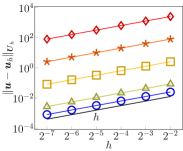
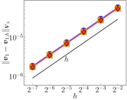
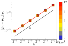
Figure 1: Error approximation of the $\text{BDM}_{1}$-$\text{BDM}_{1}$-$\text{P}_{0}$ discretization of the single network Biot-Brinkman model. Parameters $\mu=1$, $\tau=10^{-1}$, $\alpha_{1}=10^{-3}$, $c_{1}=10^{-2}$, $\nu_{1}=1$ and $K_{1}=1$ are fixed. Line colors correspond to different values of $\lambda$.

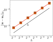
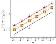
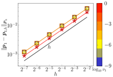
Figure 2: Error approximation of the $\text{BDM}_{1}$-$\text{BDM}_{1}$-$\text{P}_{0}$ discretization of the single network Biot-Brinkman model. Parameters $\mu=1$, $\tau=10^{-1}$, $\alpha_{1}=10^{-3}$, $c_{1}=10^{-2}$, $K_{1}=1$ and $\lambda=1$ are fixed. Line colors correspond to different values of $\nu_{1}$.

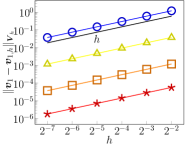
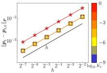
Figure 3: Error approximation of the $\text{BDM}_{1}$-$\text{BDM}_{1}$-$\text{P}_{0}$ discretization of the single network Biot-Brinkman model. Parameters $\mu=1$, $\tau=10^{-1}$, $\alpha_{1}=10^{-3}$, $c_{1}=10^{-2}$, $\nu_{1}=1$ and $\lambda=1$ are fixed. Line colors correspond to different values of $K_{1}$.

5.2 Robustness of exact preconditioner

We verify robustness of the canonical preconditioner (46) using a generalized Biot-Brinkman system with two networks. As the parameter space then counts 12 parameters in total we shall for simplicity fix material properties of one of the networks (below we choose the network $i=1$) to unity in addition to setting $\mu=1$, $\tau=1$. This choice leaves parameters $\lambda$, $c_{2}$, $\alpha_{2}$, $\nu_{2}$, $K_{2}$ as well as the transfer coefficient $\beta:=\beta_{12}$ to be varied. In the following experiments we let $1\leq\lambda\leq 10^{12}$, $10^{-9}\leq\nu_{2},K_{2},\alpha_{2}\leq 1$, $10^{-6}\leq\beta\leq 10^{6}$ and $c_{2}\in\left\{0,1\right\}$ in order to perform a systematic sensitivity study. We note that we do not vary directly the scaling parameters introduced in (19) but instead change the material parameters in (1).

For the above choice of parameters the two-network problem is considered on the domain $\Omega=(0,1)^{2}$ with boundary conditions $\bm{u}=\bm{0}$ on the left and right sides and $\left(\bm{\sigma}+\bm{\alpha}\cdot\bm{p}\bm{I}\right)\cdot\bm{n}=\bm{0}$ on the remaining part of the boundary; similarly, the Dirichlet conditions $\bm{v}_{i}\cdot\bm{n}=0$, $i=1,2$ on the fluxes are prescribed only on the left and right sides.

Having constructed spaces $\bm{U}_{h}$, $\bm{V}_{1,h}$ $\bm{V}_{2,h}$ with $\text{BDM}_{1}$ elements and pressure spaces $P_{1,h}$ $P_{2,h}$ in terms of piece-wise constants our results are summarized in Fig. 4–Fig. 6 where slices of the explored parameter space are shown. It can be seen that the condition numbers remain bounded. Concretely, given discrete operators $\mathcal{A}_{h}$, $\mathcal{B}_{h}$ that respectively discretize (19) and the preconditioner (46) the condition number is computed based on the generalized eigenvalue problem $\mathcal{A}_{h}x_{k}=\lambda_{k}\mathcal{B}^{-1}_{h}x_{k}$ as $\max_{k}\lvert\lambda_{k}\rvert/\min_{k}\lvert\lambda_{k}\rvert.$ The higher condition numbers (of about 8.5) are typically attained when $c_{2}=0$, $\lambda=1$ and $\beta\ll 1$. We remark that with $c_{2}=0$ and all parameters but $\beta$ set to 1 the condition number of $\Lambda$ ranges from $2.64$ when $\beta=10^{-6}$ to about $10^{6}$ when $\beta=10^{6}$.

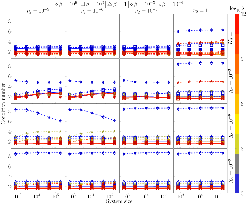
Figure 4: Performance of Biot-Brinkman preconditioner (46) for $\alpha_{2}=1$ and varying parameters $\lambda$, $\nu_{2}$, $K_{2}$, $\beta$ (denoted by markers). Binary storage capacity is considered: $c_{2}=1$ (solid lines), $c_{2}=0$ (dashed lines). The remaining parameters are fixed at 1. Discretization by $\text{BDM}_{1}$-$(\text{BDM}_{1})^{2}$-$(\text{P}_{0})^{2}$ elements. Highest condition numbers correspond to $\beta\ll 1$ and $c_{2}=0$, $\lambda=1$.

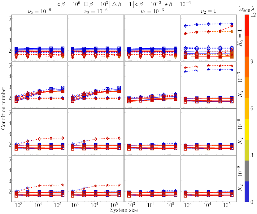
Figure 5: Performance of Biot-Brinkman preconditioner (46) for $\alpha_{2}=10^{-4}$ and varying parameters $\lambda$, $\nu_{2}$, $K_{2}$, $\beta$ (denoted by markers). Binary storage capacity is considered: $c_{2}=1$ (solid lines), $c_{2}=0$ (dashed lines). The remaining parameters are fixed at 1. Discretization by $\text{BDM}_{1}$-$(\text{BDM}_{1})^{2}$-$(\text{P}_{0})^{2}$ elements.

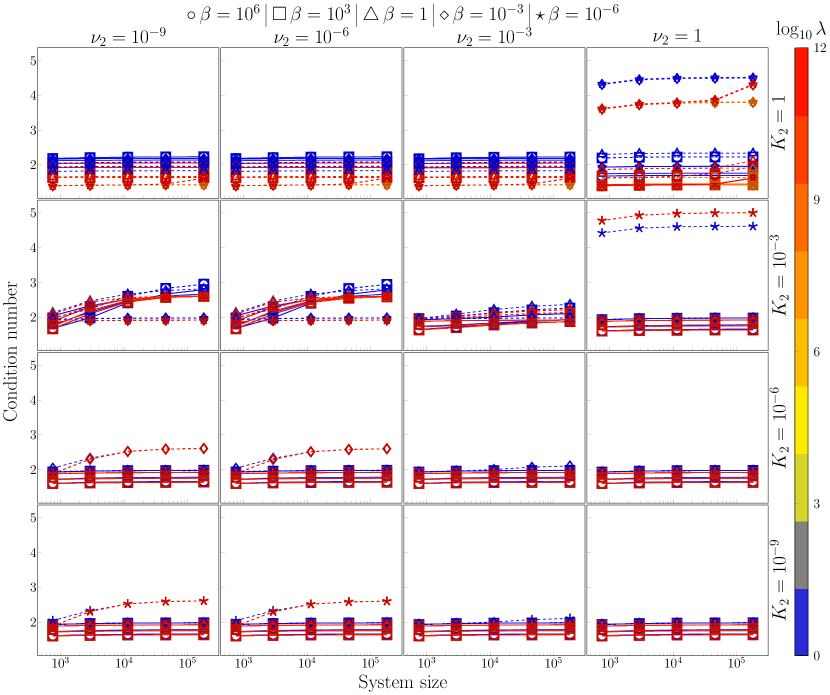
Figure 6: Performance of Biot-Brinkman preconditioner (46) for $\alpha_{2}=10^{-8}$ and varying parameters $\lambda$, $\nu_{2}$, $K_{2}$, $\beta$ (denoted by markers). Binary storage capacity is considered: $c_{2}=1$ (solid lines), $c_{2}=0$ (dashed lines). The remaining parameters are fixed at 1. Discretization by $\text{BDM}_{1}$-$(\text{BDM}_{1})^{2}$-$(\text{P}_{0})^{2}$ elements.

5.3 Multigrid preconditioning

Having seen that the exact preconditioner (46) yields parameter-robustness let us next discuss possible construction of a scalable approximation of the operator $\mathcal{B}$. Here, in order to approximate $\mathcal{B}_{\bm{u}}$ and $\mathcal{B}_{\bm{v}}$, we follow [22, 2, 19] and employ vertex-star relaxation schemes as part of geometric multigrid $F(2,2)$-cycle for the elastic block and $W(2,2)$-cycle for the flux block. Numerical experiments documenting robustness of the cycles for their respective blocks are reported in Appendix A.

To test performance of the multigrid-based preconditioner $\mathcal{B}$ we consider the two-network system from Section 5.2 where we set $c_{2}=0$, $\alpha_{2}=1$, $\beta\in\left\{10^{-6},10^{6}\right\}$ while the remaining parameters are fixed to unity. We remark that for these parameter values the highest condition numbers are attained with the exact preconditioner, cf. Fig. 4. Furthermore, differing from the setup of the sensitivity study, we (strongly) enforce $\bm{u}\cdot\bm{n}=0$ and $\bm{v}_{i}\cdot\bm{n}=0,i=1,2$, on the entire boundary. As before, the finite element discretization is based on the $\text{BDM}_{1}$ and $\text{P}_{0}$ elements.

In Fig. 7 and Fig. 8 we report the dependence on the mesh size and parameter values of the iteration counts of the preconditioned MinRes solver where as the preconditioner both the exact Riesz map (46) and the multigrid-based approximation are used. More specifically, the multigrid cycles for the displacement and flux blocks use 3 grid levels applying the exact $L^{2}$-projection as the transfer operator. For both $\mathcal{B}_{\bm{u}}$ and $\mathcal{B}_{\bm{v}}$ the vertex-star relaxation uses damped Richardson smoother. Comparing the results we observe that the use of multigrid in (46) translates to a slight (about 1.5x) increase in the number of Krylov iterations compared to the exact preconditioner. However, the iterations appear bounded in the mesh size and the parameter variations.

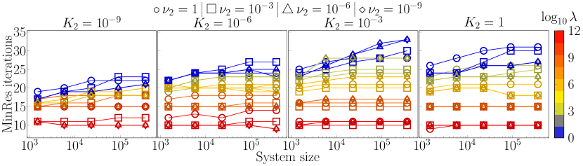
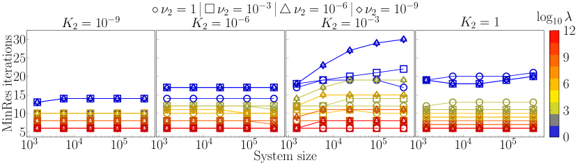
Figure 7: Number of preconditioned MinRes iterations for 2-network Biot-Brinkman system with preconditioner (46). (Top) The displacement and flux blocks use realized by geometric multigrid while $\mathcal{B}_{\bm{p}}$ is computed by LU. (Bottom) Exact (LU-inverted) preconditioner is used. Transfer coefficient $\beta=10^{6}$, while $c_{2}=0$, $\alpha_{2}=1$ and the remaining problem parameters are set to 1.

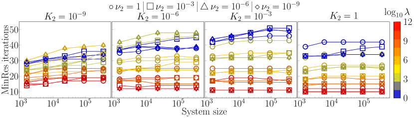
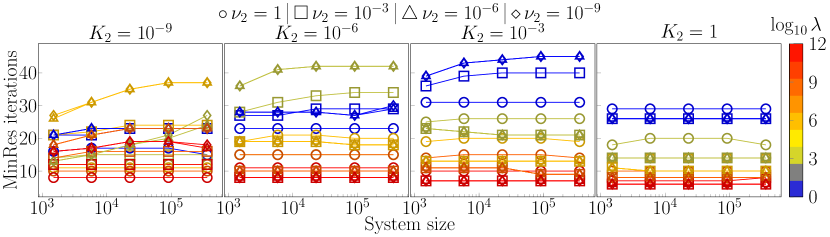
Figure 8: Number of preconditioned MinRes iterations for 2-network Biot-Brinkman system with preconditioner (46). (Top) The displacement and flux blocks use realized by geometric multigrid while $\mathcal{B}_{\bm{p}}$ is computed by LU. (Bottom) Exact preconditioner is used. Transfer coefficient $\beta=10^{-6}$, while $c_{2}=0$, $\alpha_{2}=1$ and the remaining problem parameters are set to 1.

We finally compare the cost of the exact and inexact Biot-Brinkman preconditioners for case $K_{2}=10^{-3}$, $\lambda=1$, $\beta=10^{-6}$ which required most iterations in the previous experiments, cf. Fig. 8. Our results are summarized in Table 1. We observe that despite requiring more iterations for convergence the solution time with the multigrid-based preconditioner is noticeably faster. In addition, the resulting solution algorithm appears to scale linearly in the number of unknowns. We remark that for the sake of simple comparison the computations were done in serial using single-threaded execution. However, the latter setting is particularly unfavorable for the exact preconditioner $\mathcal{B}$ as modern LU solvers are known for their thread efficiency.

	MinRes iterations LU				MinRes iterations MG
	$2^{-3}$	$2^{-4}$	$2^{-5}$	$2^{-6}$	$2^{-3}$	$2^{-4}$	$2^{-5}$	$2^{-6}$
$10^{-9}$	43	44	45	45	46	48	50	49
$10^{-6}$	43	44	45	45	46	48	50	49
$10^{-3}$	39	40	40	40	45	48	51	51
$1$	31	31	31	31	44	45	46	46
	Solve time LU [s]				Solve time MG [s]
	$2^{-3}$	$2^{-4}$	$2^{-5}$	$2^{-6}$	$2^{-3}$	$2^{-4}$	$2^{-5}$	$2^{-6}$
$10^{-9}$	2.50	4.64	23.18	181.00	4.47	7.05	18.22	64.29
$10^{-6}$	2.51	4.65	23.12	180.36	4.59	7.15	18.21	64.47
$10^{-3}$	2.50	4.64	23.06	180.34	4.57	7.05	18.24	65.45
$1$	2.51	4.57	22.74	178.84	4.45	6.94	17.63	62.83

Table 1: Performance of exact (LU) and approximate multigrid-based (MG) preconditioners for the two-network generalized Biot-Brinkman model. Parameter $\nu_{2}$ is varied while $c_{2}=0$, $K_{2}=10^{-3}$, $\beta=10^{-6}$ and the remaining parameters are set to 1. Number of unknowns in the systems ranges from $6\times 10^{3}$ to $362\times 10^{3}$. Solve time aggregates setup time of the preconditioner and the run time of the Krylov solver. Computations were done in serial with threading disabled by setting OMP_NUM_THREADS=1.

Appendix A Components of multigrid preconditioner

In this section we report numerical experiments demonstrating robustness of geometric multigrid preconditioners for blocks $\mathcal{B}_{\bm{u}}$ and $\mathcal{B}_{\bm{v}}$ of the Biot-Brinkman preconditioner (46). Adapting the unit square geometry and the setup of boundary conditions from Section 5.3 we investigate performance of the preconditioners by considering boundedness of the (preconditioned) conjugate gradient (CG) iterations. In the following, the initial vector is set to 0 and the convergence of the CG solver is determined by reduction of the preconditioned residual norm by a factor $10^{8}$. Finally, both systems are discretized by $\text{BDM}_{1}$ elements.

Table 2 confirms robustness of the $F(2,2)$-cycle for the displacement block of (46). In particular, the iterations can be seen to be bounded in mesh size and the Lamé parameter $\lambda$.

$\lambda$	$\log_{2}h$
	${-3}$	${-4}$	${-5}$	${-6}$	${-7}$	${-8}$
1	10	10	9	9	9	9
$10^{3}$	14	14	13	13	12	12
$10^{6}$	14	14	13	13	13	12
$10^{9}$	14	14	14	13	13	13
$10^{12}$	14	15	14	14	15	16

Table 2: Number of preconditioned conjugate gradient iterations for approximating the displacement block $\mathcal{B}_{\bm{u}}$ of the Biot-Brinkman preconditioner. Geometric multigrid preconditioner uses $F(2,2)$-cycle with 3 levels and a vertex-star (damped Richardson) smoother. In all experiments $\mu=1$.

For the flux block $\mathcal{B}_{\bm{v}}$ we limit the investigations to the two-network case and set $c_{2}=0$, $\alpha_{2}=1$ as these parameter values yielded the stiffest problems (in terms of their condition numbers) in the robustness study of Section 5.2. Performance of the geometric multigrid preconditioner using a $W(2,2)$-cycle with vertex-star smoother is then summarized in Figure 9. We observe that the number of CG iterations is bounded in the mesh size and variations in $K_{2}$, $\nu_{2}$ and the exchange coefficient $\beta$.

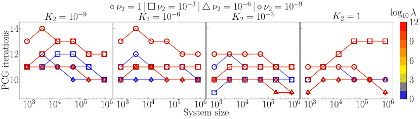
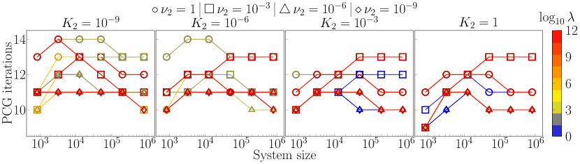
Figure 9: Number of preconditioned conjugate gradient iterations for approximating the flux block $\mathcal{B}_{\bm{v}}$ of the Biot-Brinkman preconditioner. The preconditioner uses $W(2,2)$-cycle of geometric multigrid with vertex-star (damped Richardson) smoother and 3 grid levels. (Top) Transfer coefficient $\beta=10^{6}$, (bottom) $\beta=10^{-6}$. Values of $K_{2}$, $\nu_{2}$ (encoded by markers) and $\lambda$ (encoded by line color) are varied. In both setups $c_{2}=0$, $\alpha_{2}=1$ and the remaining problem parameters are set to 1.

References

- [1] D. N. Arnold, F. Brezzi, B. Cockburn, and L. D. Marini, Unified analysis of discontinuous Galerkin methods for elliptic problems, SIAM journal on numerical analysis, 39 (2002), pp. 1749–1779.
- [2] D. N. Arnold, R. S. Falk, and R. Winther, Multigrid in H(div) and H(curl), Numerische Mathematik, 85 (2000), pp. 197–217.
- [3] F. Aznaran, R. Kirby, and P. Farrell, Transformations for Piola-mapped elements, arXiv preprint arXiv:2110.13224, (2021).
- [4] M. Bai, D. Elsworth, and J.-C. Roegiers, Multiporosity/multipermeability approach to the simulation of naturally fractured reservoirs, Water Resources Research, 29 (1993), pp. 1621–1633.
- [5] G. Barenblatt, G. Zheltov, and I. Kochina, Basic concepts in the theory of seepage of homogeneous liquids in fissured rocks [strata], J. Appl. Math. Mech., 24 (1960).
- [6] N. Barnafi, P. Zunino, L. Dedè, and A. Quarteroni, Mathematical analysis and numerical approximation of a general linearized poro-hyperelastic model, Computers & Mathematics with Applications, 91 (2021), pp. 202–228.
- [7] M. Biot, General theory of three-dimensional consolidation, J. Appl. Phys., 12 (1941), pp. 155–164.
- [8] M. Biot, Theory of elasticity and consolidation for a porous anisotropic solid, J. Appl. Phys., 26 (1955), pp. 182–185.
- [9] D. Boffi, F. Brezzi, and M. Fortin, Mixed finite element methods and applications, vol. 44 of Springer Ser. Comput. Math., Springer, Heidelberg, 2013.
- [10] F. Brezzi, On the existence, uniqueness and approximation of saddle-point problems arising from Lagrangian multipliers, Rev. Française Automat. Informat. Recherche Opérationnelle Sér. Rouge, 8 (1974), pp. 129–151.
- [11] H. C. Brinkman, A calculation of the viscous force exerted by a flowing fluid on a dense swarm of particles, Flow, Turbulence and Combustion, 1 (1949), pp. 27–34.
- [12] B. Burtschell, P. Moireau, and D. Chapelle, Numerical analysis for an energy-stable total discretization of a poromechanics model with inf-sup stability, Acta Mathematicae Applicatae Sinica, 35 (2019), pp. 28–53.
- [13] R. Chabiniok, V. Y. Wang, M. Hadjicharalambous, L. Asner, J. Lee, M. Sermesant, E. Kuhl, A. A. Young, P. Moireau, M. P. Nash, et al., Multiphysics and multiscale modelling, data–model fusion and integration of organ physiology in the clinic: ventricular cardiac mechanics, Interface focus, 6 (2016), p. 20150083.
- [14] D. Chapelle and P. Moireau, General coupling of porous flows and hyperelastic formulations—from thermodynamics principles to energy balance and compatible time schemes, European Journal of Mechanics-B/Fluids, 46 (2014), pp. 82–96.
- [15] S. Chen, Q. Hong, J. Xu, and K. Yang, Robust block preconditioners for poroelasticity, Computer Methods in Applied Mechanics and Engineering, 369 (2020), p. 113229.
- [16] D. Chou, J. Vardakis, L. Guo, B. Tully, and Y. Ventikos, A fully dynamic multi-compartmental poroelastic system: Application to aqueductal stenosis, J. Biomech., 49 (2016), pp. 2306–2312.
- [17] H. Darcy, Les fontaines publiques de la ville de Dijon: exposition et application…, Victor Dalmont, 1856.
- [18] E. Eliseussen, M. E. Rognes, and T. B. Thompson, A-posteriori error estimation and adaptivity for multiple-network poroelasticity, arXiv preprint arXiv:2111.13456, (2021).
- [19] P. E. Farrell, M. G. Knepley, L. Mitchell, and F. Wechsung, PCPATCH: Software for the topological construction of multigrid relaxation methods, ACM Trans. Math. Softw., 47 (2021), https://doi.org/10.1145/3445791.
- [20] L. Guo, J. Vardakis, T. Lassila, M. Mitolo, N. Ravikumar, D. Chou, M. Lange, A. Sarrami-Foroushani, B. Tully, Z. Taylor, S. Varma, A. Venneri, A. Frangi, and Y. Ventikos, Subject-specific multi-poroelastic model for exploring the risk factors associated with the early stages of Alzheimer’s disease, Interface Focus, 8 (2018), p. 20170019.
- [21] P. Hansbo and M. Larson, Discontinuous Galerkin and the Crouzeix-Raviart element: application to elasticity, ESAIM: Mathematical Modelling and Numerical Analysis, 37 (2003), pp. 63–72.
- [22] Q. Hong and J. Kraus, Uniformly stable discontinuous Galerkin discretization and robust iterative solution methods for the Brinkman problem, SIAM J. Numer. Anal., 54 (2016), pp. 2750–2774.
- [23] Q. Hong and J. Kraus, Parameter-robust stability of classical three-field formulation of Biot’s consolidation model, Electron. Trans. Numer. Anal., 48 (2018), pp. 202–226.
- [24] Q. Hong, J. Kraus, M. Lymbery, and F. Philo, Conservative discretizations and parameter-robust preconditioners for Biot and multiple-network flux-based poroelasticity models, Numerical Linear Algebra with Applications, 26 (2019), p. e2242.
- [25] Q. Hong, J. Kraus, M. Lymbery, and F. Philo, Parameter-robust Uzawa-type iterative methods for double saddle point problems arising in Biot’s consolidation and multiple-network poroelasticity models, Mathematical Models and Methods in Applied Sciences, 30 (2020), pp. 2523–2555.
- [26] Q. Hong, J. Kraus, M. Lymbery, and F. Philo, A new framework for the stability analysis of perturbed saddle-point problems and applications, arXiv:2103.09357v3 [math.NA], (2021).
- [27] Q. Hong, J. Kraus, M. Lymbery, and M. F. Wheeler, Parameter-robust convergence analysis of fixed-stress split iterative method for multiple-permeability poroelasticity systems, Multiscale Modeling & Simulation, 18 (2020), pp. 916–941.
- [28] Q. Hong, J. Kraus, J. Xu, and L. Zikatanov, A robust multigrid method for discontinuous Galerkin discretizations of Stokes and linear elasticity equations, Numer. Math., 132 (2016), pp. 23–49.
- [29] Q. Hong, F. Wang, S. Wu, and J. Xu, A unified study of continuous and discontinuous Galerkin methods, Science China Mathematics, 62 (2019), pp. 1–32.
- [30] J. S. Howell and N. J. Walkington, Inf–sup conditions for twofold saddle point problems, Numerische Mathematik, 118 (2011), p. 663.
- [31] R. Kedarasetti, P. J. Drew, and F. Costanzo, Arterial vasodilation drives convective fluid flow in the brain: a poroelastic model, bioRxiv, (2021).
- [32] M. Khaled, D. Beskos, and E. Aifantis, On the theory of consolidation with double porosity. 3. a finite-element formulation, (1984), pp. 101–123.
- [33] J. Kraus, P. L. Lederer, M. Lymbery, and J. Schöberl, Uniformly well-posed hybridized discontinuous Galerkin/hybrid mixed discretizations for Biot’s consolidation model, Comput. Methods Appl. Mech. Engrg., 384 (2021), pp. Paper No. 113991, 23, https://doi.org/10.1016/j.cma.2021.113991, https://doi.org/10.1016/j.cma.2021.113991.
- [34] S. Kumar, R. Oyarzúa, R. Ruiz-Baier, and R. Sandilya, Conservative discontinuous finite volume and mixed schemes for a new four-field formulation in poroelasticity, ESAIM Math. Model. Numer. Anal., 54 (2020), pp. 273–299, https://doi.org/10.1051/m2an/2019063, https://doi.org/10.1051/m2an/2019063.
- [35] J. Lee, K.-A. Mardal, and R. Winther, Parameter-robust discretization and preconditioning of Biot’s consolidation model, SIAM J. Sci. Comput., 39 (2017), pp. A1–A24, https://doi.org/10.1137/15M1029473, http://dx.doi.org/10.1137/15M1029473.
- [36] J. J. Lee, E. Piersanti, K.-A. Mardal, and M. E. Rognes, A mixed finite element method for nearly incompressible multiple-network poroelasticity, SIAM Journal on Scientific Computing, 41 (2019), pp. A722–A747.
- [37] K.-A. Mardal, M. E. Rognes, and T. B. Thompson, Accurate discretization of poroelasticity without Darcy stability, BIT Numerical Mathematics, (2021), pp. 1–36.
- [38] M. P. Nash and P. J. Hunter, Computational mechanics of the heart, Journal of elasticity and the physical science of solids, 61 (2000), pp. 113–141.
- [39] E. Piersanti, J. J. Lee, T. Thompson, K.-A. Mardal, and M. E. Rognes, Parameter robust preconditioning by congruence for multiple-network poroelasticity, SIAM Journal on Scientific Computing, 43 (2021), pp. B984–B1007.
- [40] K. R. Rajagopal, On a hierarchy of approximate models for flows of incompressible fluids through porous solids, Mathematical Models and Methods in Applied Sciences, 17 (2007), pp. 215–252.
- [41] F. Rathgeber, D. A. Ham, L. Mitchell, M. Lange, F. Luporini, A. T. T. Mcrae, G.-T. Bercea, G. R. Markall, and P. H. J. Kelly, Firedrake: Automating the finite element method by composing abstractions, ACM Trans. Math. Softw., 43 (2016), https://doi.org/10.1145/2998441.
- [42] C. Rodrigo, X. Hu, P. Ohm, J. H. Adler, F. J. Gaspar, and L. Zikatanov, New stabilized discretizations for poroelasticity and the Stokes’ equations, Computer Methods in Applied Mechanics and Engineering, 341 (2018), pp. 467–484.
- [43] R. Showalter, Poroelastic filtration coupled to Stokes flow, Lecture Notes in Pure and Appl. Math., 242 (2010), pp. 229–241.
- [44] K. H. Støverud, M. Alnæs, H. P. Langtangen, V. Haughton, and K.-A. Mardal, Poro-elastic modeling of Syringomyelia–a systematic study of the effects of pia mater, central canal, median fissure, white and gray matter on pressure wave propagation and fluid movement within the cervical spinal cord, Computer methods in biomechanics and biomedical engineering, 19 (2016), pp. 686–698.
- [45] B. Tully and Y. Ventikos, Cerebral water transport using multiple-network poroelastic theory: application to normal pressure hydrocephalus, J. Fluid Mech., 667 (2011), pp. 188–215.
- [46] J. Vardakis, D. Chou, B. Tully, C. Hung, T. Lee, P. Tsui, and Y. Ventikos, Investigating cerebral oedema using poroelasticity, Med. Eng. Phys., 38 (2016), pp. 48–57.
- [47] S. Whitaker, Flow in porous media I: A theoretical derivation of Darcy’s law, Transport in porous media, 1 (1986), pp. 3–25.
- [48] R. Wilson and E. Aifantis, On the theory of consolidation with double porosity, 20 (1982), pp. 1009–1035.