Linear and nonlinear optical properties from TDOMP2 theory

Abstract

We present a derivation of the real-time time-dependent orbital-optimized Møller-Plesset (TDOMP2) theory and its biorthogonal companion, time-dependent non-orthogonal OMP2 (TDNOMP2), theory starting from the time-dependent bivariational principle and a parametrization based on the exponential orbital-rotation operator formulation commonly used in time-independent molecular electronic-structure theory. We apply the TDOMP2 method to extract absorption spectra and frequency-dependent polarizabilities and first hyperpolarizabilities from real-time simulations, comparing the results with those obtained from conventional time-dependent coupled-cluster singles and doubles (TDCCSD) simulations and from its second-order approximation TDCC2. We also compare with results from CCSD and CC2 linear and quadratic response theory. Our results indicate that while TDOMP2 absorption spectra are of the same quality as TDCC2 spectra, including core excitations where optimized orbitals might be particularly important, frequency-dependent polarizabilities and hyperpolarizabilities from TDOMP2 simulations are significantly closer to TDCCSD results than those from TDCC2 simulations.

Hylleraas Centre] Hylleraas Centre for Quantum Molecular Sciences, Department of Chemistry, University of Oslo, N-0315 Oslo, Norway [Simula]Simula Research Laboratory, Kristian Augusts gate 23, 0164 Oslo, Norway Hylleraas Centre] Hylleraas Centre for Quantum Molecular Sciences, Department of Chemistry, University of Oslo, N-0315 Oslo, Norway CAS] Centre for Advanced Study at the Norwegian Academy of Science and Letters, Drammensveien 78, N-0271 Oslo, Norway [Hylleraas Centre] Hylleraas Centre for Quantum Molecular Sciences, Department of Chemistry, University of Oslo, N-0315 Oslo, Norway CAS] Centre for Advanced Study at the Norwegian Academy of Science and Letters, Drammensveien 78, N-0271 Oslo, Norway [Hylleraas Centre] Hylleraas Centre for Quantum Molecular Sciences, Department of Chemistry, University of Oslo, N-0315 Oslo, Norway

1 Introduction

The correct semiclassical description of interactions between matter and temporally oscillating electromagnetic fields must start from time-dependent quantum mechanics. Historically, the most-often used approach within molecular electronic-structure theory has been time-dependent perturbation theory where the time-dependent Schrödinger equation is solved order by order in the external field strength, leading to response theory of molecular properties in the frequency domain through the application of a series of Fourier transforms. ¹ Response theory has the advantage that it directly addresses the quantities that are used for the interpretation of experimental measurements, such as one- and two-photon transition moments and frequency-dependent electric-dipole polarizabilities and hyperpolarizabilities, which may be expressed in terms of transition energies and stationary-state wave functions that can, at least in principle, be obtained from the time-independent Schrödinger equation for the particle system alone. A major disadvantage is that time resolution is lost when going from the time domain to the frequency domain. The obvious solution would be to skip the Fourier transforms and instead work directly in the time domain. This, however, implies that the time-dependent Schrödinger equation must be solved order by order in a discretized time series, making the approach much too computationally demanding for higher-order properties. Instead, so-called real-time methods have received increasing attention in recent years—see, e.g., the review of real-time time-dependent electronic-structure theory by Li et al. ²

Real-time (RT) methods approximate the solution of the time-dependent Schrödinger equation without perturbation expansions and, thus, contain information about the response of the atomic or molecular electrons to external electromagnetic fields to all orders in perturbation theory. Even extremely nonlinear processes that are practically out of reach within response theory, such as high harmonic generation and time-resolved one- and many-electron ionization probability amplitudes, are accessible with RT methods, see Ref. 2 and references therein. Moreover, since RT methods include the field explicitly in the simulation, it becomes possible to investigate the detailed dependence on laser parameters such as intensity, frequency distribution, pulse shape, and delay between pump and probe pulses without making explicit assumptions about the perturbation order of the electronic processes involved.

While RT methods are usually much simpler to implement than response theory (typically, the same code is needed as for ground-state calculations, only generalized to complex parameters), a major downside of RT methods is the increased computational cost arising from the discretization of time. Thousands or even hundreds of thousands of time steps are needed, each associated with a cost comparable to one (or a few) iterations of a ground-state optimization with the same (time-independent) method. In addition, the basis-set requirements are generally more demanding since, in principle, all excited states and even continuum states may be involved in the dynamics, and acceleration techniques commonly used for ground-state and response calculations may not be generally applicable for RT simulations with all possible external electromagnetic fields.

It is no surprise, therefore, that the most widely used RT electronic-structure method is real-time time-dependent density-functional theory (RT-TDDFT) ^{2, 3, 4, 5}. Highly accurate wave function-based RT methods have also been developed, including multiconfigurational time-dependent Hartree-Fock (MCTDHF) ^{6, 7, 8, 9} theory and related complete, restricted, and generalized active space formulations ^{10, 11, 12}. Avoiding the factorial computational scaling caused by the full configuration interaction (FCI) treatment at the heart of these approaches, time-dependent extensions of single-reference coupled-cluster (CC) theory ¹³ and equation-of-motion CC (EOM-CC) theory ^{14, 15} have been increasingly often used to simulate laser-driven many-electron dynamics in the time domain in recent years ^{16, 17, 18, 19, 20, 21, 22, 23, 24, 25, 26, 27, 28, 29, 30, 31, 32, 33}. The two approaches, time-dependent CC (TDCC) and time-dependent EOM-CC (TD-EOM-CC) theory, differ in their parametrization of the time-dependent left and right wave functions. While TDCC theory propagates the well-known exponential Ansätze for the wave functions, TD-EOM-CC theory expresses them as linear combinations of EOM-CC left and right eigenstates. While both approaches are expected to give similar results (and, indeed, appear to do so, see Ref. 33) for weak-field processes, only TDCC theory (albeit with dynamical orbitals) has been successfully applied to strong-field phenomena such as ionization dynamics and high harmonic generation ²⁰ to date.

Although the original formulation of TDCC theory in nuclear physics was based on time-dependent Hartree-Fock (HF) orbitals, ³⁴ conventional TDCC theory is formulated with a static reference determinant, the HF ground state, which is kept fixed during the dynamics in agreement with the conventional formulation of CC response (LRCC) theory ^{35, 36}. The fixed orbital space has some unwanted side effects, however. Gauge invariance is lost in truncated TDCC theory (but recovered in the FCI limit) ^{37, 38}, severe numerical challenges arise as the CC ground state is depleted during the dynamics (e.g., in ground–excited state Rabi oscillations) ^{21, 29}, and it becomes impossible to reduce the computational effort whilst maintaining accuracy by splitting the orbital space into active and inactive orbitals for the correlated treatment, as required to efficiently describe ionization dynamics ¹⁷. These deficiencies can, at least partially, be circumvented by allowing the orbitals to move in concert with the electron correlation. In practice, this is done by replacing the single excitations (and de-excitations) of conventional CC theory with full orbital rotations. This, in turn, can be done in two ways. Within orbital-optimized CC (OCC) theory ^{39, 40, 37}, the orbitals are required to remain orthonormal, whereas within nonorthogonal orbital-optimized CC (NOCC) theory ^{38, 17} they are only required to be biorthonormal. The orthonormality constraint has an unfortunate side effect in the sense that OCC theory does not converge to the FCI solution in the limit of full rank cluster operators for three or more electrons, as pointed out by Köhn and Olsen ⁴¹. On the other hand, Myhre ⁴² recently showed that NOCC theory may converge to the correct FCI limit for any number of electrons. In practice, however, time-dependent OCC (TDOCC) theory does not appear to deviate from the FCI limit by any significant amount ²⁰.

The computational scaling with respect to the size of the basis set and with respect to the number of electrons of TDOCC and time-dependent NOCC (TDNOCC) theory is essentially identical to that of conventional TDCC theory with identical truncation of the cluster operators. The lowest-level truncation, after double excitations, yields the TDOCCD and TDNOCCD methods that both scale as $\mathcal{O}(N^{6})$, which is significantly more expensive than the formal $\mathcal{O}(N^{4})$ scaling of RT-TDDFT. In order to bring down the computational cost to a more tractable level, Pathak et al. ^{26, 27} generalized the orbital-optimized second-order Møller-Plesset (OMP2) ⁴³ method to the time domain and demonstrated that the resulting TDOMP2 method provides a reasonably accurate and gauge invariant description of highly nonlinear optical processes.

In this work we assess the description of linear and quadratic optical properties within the TDOMP2 approximation. First, we review TDCC theory and its second-order approximation TDCC2. Second, we review time-dependent coupled-cluster theories with dynamic orbitals—TDNOCC and TDOCC theory—as obtained from the time-dependent bivariational principle, and introduce the second-order approximations TDNOMP2 and TDOMP2. Finally, we compute linear (one-photon) absorption spectra and frequency-dependent polarizabilities and first hyperpolarizabilities with the TDOMP2, TDCCSD, and TDCC2 methods, and compare with results from CC2 and CCSD linear and quadratic response theory.

2 Theory

2.1 Notation

We consider a system of $N$ interacting electrons described by the second-quantized Hamiltonian

$$\hat{H}=\sum_{pq}h^{p}_{q}\hat{a}_{p}^{\dagger}\hat{a}_{q}+\frac{1}{2}\sum_{pqrs}u^{pq}_{rs}\hat{a}_{p}^{\dagger}\hat{a}_{q}^{\dagger}\hat{a}_{s}\hat{a}_{r}=\sum_{pq}h^{p}_{q}\hat{a}_{p}^{\dagger}\hat{a}_{q}+\frac{1}{4}\sum_{pqrs}v^{pq}_{rs}\hat{a}_{p}^{\dagger}\hat{a}_{q}^{\dagger}\hat{a}_{s}\hat{a}_{r},$$ (1)

where $\hat{a}_{p}^{\dagger}$ ($\hat{a}_{p}$) are creation (annihilation) operators associated with a finite set of $L$ orthonormal spin orbitals $\{\phi_{p}\}_{p=1}^{L}$. The one- and two-body matrix elements $h^{p}_{q}$ and $u^{pq}_{rs}$ are defined as

$$h^{p}_{q} =\braket{\phi_{p}}{\hat{h}}{\phi_{q}}=\int\phi_{p}^{*}(\mathbf{x}_{1})\hat{h}(1)\phi_{q}(\mathbf{x}_{1})\,d\mathbf{x}_{1},$$ (2)

$$u^{pq}_{rs} =\braket{\phi_{p}\phi_{q}}{\hat{u}}{\phi_{r}\phi_{s}}=\iint\phi_{p}^{*}(\mathbf{x}_{1})\phi_{q}^{*}(\mathbf{x}_{2})\hat{u}(1,2)\phi_{r}(\mathbf{x}_{1})\phi_{s}(\mathbf{x}_{2})\,d\mathbf{x}_{1}\,d\mathbf{x}_{2},$$ (3)

where $\mathbf{x}_{i}=(\mathbf{r}_{i},\sigma_{i})$ refers to the combined spatial-spin coordinate of electron $i$. The anti-symmetrized two-body matrix elements $v^{pq}_{rs}$ are given by

$$v^{pq}_{rs}=u^{pq}_{rs}-u^{pq}_{sr}.$$ (4)

2.2 The TDCC2 approximation

The TDCC Ansätze for the left and right coupled-cluster wave functions are defined by

$$\ket{\Psi(t)}=e^{\hat{T}(t)}\ket{\Phi_{0}},\qquad\bra{\tilde{\Psi}(t)}=\bra{\Phi_{0}}\hat{\Lambda}(t)e^{-\hat{T}(t)},$$ (5)

where $\ket{\Phi_{0}}$ is a reference determinant built from orthonormal spin orbitals, typically taken as the HF ground-state determinant. The chosen reference determinant splits the orbital set into occupied orbitals denoted by subscripts $i,j,k,l$ and virtual orbitals denoted by subscripts $a,b,c,d$. Subscripts $p,q,r,s$ are used to denote general orbitals. The cluster operators $\hat{T}(t)$ and $\hat{\Lambda}(t)$ are given by

$$\hat{T}(t) =\sum_{\mu}\tau^{\mu}(t)\hat{X}_{\mu}=\hat{T}_{0}+\hat{T}_{1}+\hat{T}_{2}+\hat{T}_{3}+\cdots+\hat{T}_{N},$$ (6)

$$\hat{\Lambda}(t) =\sum_{\mu}\lambda_{\mu}(t)\hat{Y}^{\mu}=\hat{\Lambda}_{0}+\hat{\Lambda}_{1}+\hat{\Lambda}_{2}+\hat{\Lambda}_{3}+\cdots+\hat{\Lambda}_{N},$$ (7)

where $\mu$ denotes excitations of rank $0,1,2,3,\ldots,N$, and the excitation and de-excitation operators $\hat{X}_{\mu}$ and $\hat{Y}^{\mu}$ are defined by

$$\hat{X}_{0} \equiv 1,\qquad\hat{X}_{\mu}\ket{\Phi_{0}}\equiv\ket{\Phi_{\mu}},$$ (8)

$$\hat{Y}^{0} \equiv 1,\qquad\bra{\Phi_{0}}\hat{Y}^{\mu}\equiv\bra{\tilde{\Phi}_{\mu}},$$ (9)

such that $\braket{\tilde{\Phi}_{\mu}}{\Phi_{\nu}}=\delta_{\mu\nu}$. The rank-$0$ cluster operators are included to describe the phase and (intermediate) normalization of the CC state ²¹.

The equations of motion for the wave function parameters are obtained from the bivariational action functional used by Arponen ⁴⁴

$$\mathcal{S}[\tilde{\Psi},\Psi]=\int_{t_{0}}^{t_{1}}\mathcal{L}\,dt,$$ (10)

where the CC Lagrangian is given by

$$\mathcal{L}=\braket{\tilde{\Psi}(t)}{\hat{H}(t)-i\partial_{t}}{\Psi(t)}=\mathcal{H}-i\sum_{\mu}\lambda_{\mu}\dot{\tau}^{\mu},$$ (11)

and the Hamilton function $\mathcal{H}$ is given by

$$\mathcal{H}=\braket{\tilde{\Psi}(t)}{\hat{H}(t)}{\Psi(t)}.$$ (12)

The requirement that $\mathcal{S}[\tilde{\Psi},\Psi]$ be stationary with respect to variations of the complex parameters $z_{\mu}\in\{\tau^{\mu},\lambda_{\mu}\}$ leads to the Euler-Lagrange equations

$$\frac{\partial\mathcal{L}}{\partial z_{\mu}}=\frac{d}{dt}\frac{\partial\mathcal{L}}{\partial\dot{z}_{\mu}}.$$ (13)

Taking the required derivatives yields the equations of motion for the amplitudes,

$$i\dot{\tau}^{\mu}(t) =\braket{\Phi_{0}}{\hat{Y}^{\mu}e^{-\hat{T}(t)}\hat{H}(t)e^{\hat{T}(t)}}{\Phi_{0}},$$ (14)

$$-i\dot{\lambda}_{\mu}(t) =\braket{\Phi_{0}}{\hat{\Lambda}(t)e^{-\hat{T}(t)}[\hat{H}(t),\hat{X}_{\mu}]e^{\hat{T}(t)}}{\Phi_{0}}.$$ (15)

Note that $\lambda_{0}(t)$ is a constant, which we choose such that the intermediate normalization condition $\braket{\tilde{\Psi}(t)}{\Psi(t)}=1$ is satisfied, whereas the phase amplitude $\tau_{0}$ generally depends nontrivially on time ²¹. The phase amplitude may, however, be ignored as long as we are only interested in the time evolution of expectation values ³⁵. For other quantities, such as the autocorrelation of the CC state ²¹ or certain stationary-state populations ³⁰, the phase amplitude is needed. In the present work, we will only consider expectation values.

Truncation of the cluster operators after single and double excitations defines the TDCCSD method, which has an asymptotic scaling of $\mathcal{O}(N^{6})$. Defined as a second-order approximation to the TDCCSD method within many-body perturbation theory, the TDCC2 method ⁴⁵ reduces the asymptotic scaling to $\mathcal{O}(N^{5})$. In order to derive the TDCC2 equations, we partition the time-dependent Hamiltonian

$$\hat{H}(t)=\hat{H}^{(0)}(t)+\hat{U}$$ (16)

into a zeroth-order term, $\hat{H}^{(0)}(t)=\hat{f}+\hat{V}(t)$, where $\hat{f}$ is the Fock operator, and

$$\hat{V}(t)=\sum_{pq}(V)^{p}_{q}(t)\hat{a}_{p}^{\dagger}\hat{a}_{q}$$ (17)

is a time-dependent one-electron operator representing the interaction with an external field. The first-order term (the fluctuation potential) is defined as,

$$\hat{U}=\hat{H}(t)-\hat{f}-\hat{V}(t).$$ (18)

In the many-body perturbation analysis of the TDCCSD equations, the singles and doubles amplitudes are considered zeroth-order and first-order quantities, respectively. For notational convenience the time-dependence of the amplitudes and operators will be understood implicitly in the following.

Equations of motion are obtained from making the action given by Eq. (10) stationary with respect to variations of the amplitudes. The TDCC2 Lagrangian is obtained from the TDCCSD Lagrangian by retaining terms up to quadratic in the doubles amplitudes and the fluctuation potential,

$$\mathcal{L}=\mathcal{H}-i\left(\sum_{\mu_{1}}\lambda_{\mu_{1}}\dot{\tau}^{\mu_{1}}+\sum_{\mu_{2}}\lambda_{\mu_{2}}\dot{\tau}^{\mu_{2}}\right).$$ (19)

Introducing $\hat{T}_{1}$-transformed operators as

$$\tilde{\Omega}=e^{-\hat{T}_{1}}\hat{\Omega}e^{\hat{T}_{1}},$$ (20)

the TDCC2 approximation to the TDCCSD Hamilton function becomes

$$\mathcal{H} =\bra{\Phi_{0}}e^{-\hat{T}_{2}}\tilde{H}e^{\hat{T}_{2}}\ket{\Phi_{0}}$$

$$+\sum_{\mu_{1}}\lambda_{\mu_{1}}\bra{\tilde{\Phi}_{\mu_{1}}}\tilde{H}+[\tilde{H},\hat{T}_{2}]\ket{\Phi_{0}}+\sum_{\mu_{2}}\lambda_{\mu_{2}}\bra{\tilde{\Phi}_{\mu_{2}}}[\hat{f}+\tilde{V},\hat{T}_{2}]+\tilde{U}\ket{\Phi_{0}}.$$ (21)

Note that the Fock operator appearing in the commutator in the last term is not $\hat{T}_{1}$ transformed. The Euler-Lagrange equations then yield equations of motion for the singles amplitudes,

$$i\dot{\lambda}^{i}_{a} =(f_{1})^{i}_{a}+(f_{1})^{b}_{a}\lambda^{i}_{b}-(f_{1})^{i}_{j}\lambda^{j}_{a}+\lambda^{j}_{b}\tilde{v}^{ib}_{aj}+\frac{1}{2}\sum_{c}\lambda^{ij}_{bc}\tilde{v}^{bc}_{aj}-\frac{1}{2}\sum_{k}\lambda^{jk}_{ab}\tilde{v}^{ib}_{jk}$$

$$+\sum_{ck}\left(\lambda^{j}_{b}\tau^{bc}_{jk}\tilde{v}^{ik}_{ac}-\frac{1}{2}\lambda^{i}_{b}\tau^{bc}_{jk}\tilde{v}^{jk}_{ac}-\frac{1}{2}\lambda^{j}_{a}\tau^{bc}_{jk}\tilde{v}^{ik}_{bc}\right),$$ (22)

$$i\dot{\tau}^{a}_{i} =(f_{1})^{a}_{i}+\sum_{jb}(f_{1})^{j}_{b}\tau_{ji}^{ba}+\frac{1}{2}\sum_{jbc}\tau_{ik}^{bc}\tilde{v}^{aj}_{bc}+\frac{1}{2}\sum_{jkc}\tau_{jk}^{ac}\tilde{v}^{jk}_{bi},$$ (23)

and for the doubles amplitudes,

$$i\dot{\tau}^{ab}_{ij} =\tilde{v}^{ij}_{ab}+P(ab)\sum_{c}(f_{2})^{a}_{c}\tau_{ij}^{cb}+P(ij)\sum_{k}(f_{2})^{k}_{j}\tau_{ki}^{ab},$$ (24)

$$i\dot{\lambda}^{ij}_{ab} =\tilde{v}^{ij}_{ab}+\hat{P}(ab)\hat{P}(ij)(f_{1})^{i}_{a}\lambda^{j}_{b}-\sum_{c}\left(\hat{P}(ab)(f_{2})^{c}_{a}\lambda^{ij}_{bc}+\hat{P}(ij)\lambda^{i}_{c}\tilde{v}^{jc}_{ab}\right)$$

$$+\sum_{k}\left(\hat{P}(ij)(f_{2})^{i}_{k}\lambda^{jk}_{ab}+\hat{P}(ab)\lambda^{k}_{a}\tilde{v}^{ij}_{bk}\right).$$ (25)

Here, we have defined the fully and partially $T_{1}$-transformed Fock matrices

$$(f_{1})^{p}_{q}\equiv\tilde{f}^{p}_{q}+(\tilde{V})^{p}_{q},\qquad(f_{2})^{p}_{q}\equiv f^{p}_{q}+(\tilde{V})^{p}_{q},$$ (26)

and the operator $\hat{P}(pq)$ is an anti-symmetrizer defined by its action on the elements of an arbitray tensor $M$: $\hat{P}(pq)M_{pq}=M_{pq}-M_{qp}$.

The presence of the untransformed Fock operator in Eq. (21) has a number of simplifying consequences. For example, the ground-state doubles amplitudes become explicit functions of the singles amplitudes and the double excitation block of the EOM-CC Hamiltonian matrix (the CC Jacobian) becomes diagonal. In TDCC2 theory, however, it implies that the doubles amplitudes are not fully adjusted to the approximate orbital relaxation captured by the (zeroth order) singles amplitudes. In order to test the consequences of this, we have implemented the TDCC2-b method of Kats et al. ⁴⁶, where the fully $T_{1}$-transformed Fock operator is used in Eq. (21).

2.3 Review of time-dependent coupled-cluster theories with dynamic orbitals

The TDOCC and TDNOCC Ansätze replace the singles amplitudes of conventional TDCC theory with unitary and non-unitary orbital rotations, respectively. For both types of orbital rotations, the left and right coupled-cluster wave functions can be written on the form

$$\ket{\Psi(t)}=e^{\hat{\kappa}(t)}e^{\hat{T}(t)}\ket{\Phi_{0}},\qquad\bra{\tilde{\Psi}(t)}=\bra{\Phi_{0}}\hat{\Lambda}(t)e^{-\hat{T}(t)}e^{-\hat{\kappa}(t)},$$ (27)

where $\ket{\Phi_{0}}$ is a static reference determinant built from orthonormal spin orbitals, typically taken as the HF ground-state determinant in analogy with conventional TDCC theory. The terminology of occupied and virtual orbitals thus refers to this reference determinant, although both subsets are changed by the time-dependent orbital rotations. Excluding singles amplitudes, the cluster operators $\hat{T}(t)$ and $\hat{\Lambda}(t)$ are given by

$$\hat{T}(t) =\sum_{\mu}\tau^{\mu}(t)\hat{X}_{\mu}=\hat{T}_{0}+\hat{T}_{2}+\hat{T}_{3}+\cdots+\hat{T}_{N},$$ (28)

$$\hat{\Lambda}(t) =\sum_{\mu}\lambda_{\mu}(t)\hat{Y}^{\mu}=\hat{\Lambda}_{0}+\hat{\Lambda}_{2}+\hat{\Lambda}_{3}+\cdots+\hat{\Lambda}_{N},$$ (29)

where $\mu$ denotes excitations of rank $0,2,3,\ldots,N$, and the excitation and de-excitation operators $\hat{X}_{\mu}$ and $\hat{Y}^{\mu}$ are defined the same way as in conventional TDCC theory [Eqs. (8) and (9)]. The exclusion of singles amplitudes is rigorously justified, as they become redundant when the orbitals are properly relaxed by the orbital-rotation operator $\exp(\hat{\kappa})$ ^{37, 38, 17}.

In TDNOCC theory, the orbital rotations are non-unitary, i.e. $\hat{\kappa}^{\dagger}\neq-\hat{\kappa}$. If $\hat{\kappa}$ is restricted to be anti-Hermitian, we obtain TDOCC theory where the orbital rotations are unitary. However, this leads to the parametrization formally not converging to the FCI limit (for $N>2$), as pointed out by Köhn and Olsen ⁴¹. On the other hand, Myhre ⁴² showed that the proper FCI limit may be restored by non-unitary orbital rotations. Furthermore, it can be shown that occupied-occupied and virtual-virtual rotations are redundant ^{37, 17} and it is sufficient to consider $\hat{\kappa}(t)$ on the form

$$\hat{\kappa}(t)=\sum_{ai}\left(\kappa^{a}_{i}(t)\hat{X}^{a}_{i}+\kappa^{i}_{a}(t)\hat{Y}^{i}_{a}\right).$$ (30)

Using the Baker-Campbell-Hausdorff expansion, one can show that the similarity transforms of the creation and annihilation operators with $\exp(\hat{\kappa})$ are given by

$$e^{-\hat{\kappa}(t)}\hat{a}_{p}^{\dagger}e^{\hat{\kappa}(t)} =\sum_{q}\hat{a}_{q}^{\dagger}[e^{-\kappa(t)}]^{q}_{p},$$ (31)

$$e^{-\hat{\kappa}(t)}\hat{a}_{p}e^{\hat{\kappa}(t)} =\sum_{q}\hat{a}_{q}[e^{\kappa(t)}]^{p}_{q}.$$ (32)

Recalling that explicit time-dependence only appears in the interaction operator and in the wave function parameters, we will suppress the dependence on time in the notation. For a general one- and two-body operator $\hat{\Omega}$, the TDNOCC and TDOCC expectation value functionals can be written as

$$\braket{\tilde{\Psi}(t)}{\hat{\Omega}}{\Psi(t)}=\sum_{pq}\tilde{\Omega}^{p}_{q}\gamma^{q}_{p}+\frac{1}{4}\sum_{pqrs}\tilde{\Omega}^{pq}_{rs}\Gamma^{rs}_{pq},$$ (33)

where

$$\tilde{\Omega}^{p}_{q} =\sum_{rs}[e^{-\kappa}]^{p}_{r}\Omega^{r}_{s}[e^{\kappa}]^{s}_{q},$$ (34)

$$\tilde{\Omega}^{pq}_{rs} =\sum_{tuvw}[e^{-\kappa}]^{p}_{t}[e^{-\kappa}]^{q}_{u}\Omega^{tu}_{vw}[e^{\kappa}]^{v}_{r}[e^{\kappa}]^{w}_{s},$$ (35)

and $\gamma,\Gamma$ are effective one- and two-body density matrices given by

$$\gamma^{q}_{p} =\braket{\Phi_{0}}{\hat{\Lambda}(t)e^{-\hat{T}(t)}\hat{a}_{p}^{\dagger}\hat{a}_{q}e^{\hat{T}(t)}}{\Phi_{0}},$$ (36)

$$\Gamma_{pq}^{rs} =\braket{\Phi_{0}}{\hat{\Lambda}(t)e^{-\hat{T}(t)}\hat{a}_{p}^{\dagger}\hat{a}_{q}^{\dagger}\hat{a}_{s}\hat{a}_{r}e^{\hat{T}(t)}}{\Phi_{0}}.$$ (37)

The equations of motion for the wave function parameters are, again, obtained from the Euler-Lagrange equations (13) for the full parameter set $z_{\mu}\in\{\tau^{\mu},\lambda_{\mu},\kappa^{a}_{i},\kappa^{i}_{a}\}$ with the Lagrangian given by

$$\mathcal{L} =\braket{\tilde{\Psi}}{\hat{H}-i\partial_{t}}{\Psi}$$

$$=\mathcal{H}-i\braket{\tilde{\Psi}}{\hat{Q}_{1}}{\Psi}-i\sum_{\mu}\lambda_{\mu}\dot{\tau}^{\mu},$$ (38)

where the Hamiltonian is given by Eq. (1). Here, the interaction with the external field (17) is absorbed into the one-body part of the Hamiltonian such that

$$h^{p}_{q}\leftarrow h^{p}_{q}+(V)^{p}_{q}(t).$$ (39)

The operator $\hat{Q}_{1}$ is defined as

$$\hat{Q}_{1}\equiv\frac{\partial e^{\hat{\kappa}}}{\partial t}e^{-\hat{\kappa}},$$ (40)

and $\mathcal{H}=\braket{\tilde{\Psi}}{\hat{H}(t)}{\Psi}$.

The detailed derivation of the equations of motion is greatly simplified by absorbing the orbital rotation in the Hamiltonian at each point in time, $\hat{H}\leftarrow\exp(-\hat{\kappa})\hat{H}\exp(\hat{\kappa})$, which amounts to temporally local updates of the Hamiltonian integrals according to Eqs. (34) and (35). This allows us to compute the temporally local derivatives of the Lagrangian with respect to the parameters at the point $\hat{\kappa}=0$ such that, for example, the rather complicated operator $\hat{Q}_{1}$ becomes the much simpler operator $\hat{\dot{\kappa}}$. We thus find that the equations of motion for the cluster amplitudes are given by

$$i\dot{\tau}^{\mu} =\braket{\Phi_{0}}{\hat{Y}^{\mu}e^{-\hat{T}}\left(\hat{H}-i\hat{\dot{\kappa}}\right)e^{\hat{T}}}{\Phi_{0}},$$ (41)

$$-i\dot{\lambda}_{\mu} =\braket{\Phi_{0}}{\hat{\Lambda}e^{-\hat{T}}\left[\left(\hat{H}-i\hat{\dot{\kappa}}\right),\hat{X}_{\mu}\right]e^{\hat{T}}}{\Phi_{0}},$$ (42)

where the right-hand sides are essentially identical to the usual amplitude equations of coupled-cluster theory with additional terms arising from the one-body operator $\hat{\dot{\kappa}}$. As in conventional TDCC theory, $\lambda_{0}$ is constant and may be chosen such that intermediate normalization is preserved ²¹. In the same manner, we may derive the equations of motion for the orbital-rotation parameters as

$$i\sum_{bj}\dot{\kappa}^{j}_{b}A^{ib}_{aj}=R^{i}_{a},$$ (43)

$$-i\sum_{bj}\dot{\kappa}^{b}_{j}A^{ja}_{bi}=R^{a}_{i},$$ (44)

where the right-hand sides are given by Eqs. (30a) and (30b) in Ref. 17, and

$$A^{ib}_{aj}=\braket{\tilde{\Psi}}{[\hat{a}_{j}^{\dagger}\hat{a}_{b},\hat{a}_{a}^{\dagger}\hat{a}_{i}]}{\Psi}=\delta^{b}_{a}\gamma^{i}_{j}-\delta^{i}_{j}\gamma^{b}_{a}.$$ (45)

Equations (43) and (44) are linear systems of algebraic equations which require the matrix $A=[A^{ib}_{aj}]$ to be non-singular in order to have a unique solution. We remark that this matrix becomes singular whenever an eigenvalue of the occupied density block is equal to an eigenvalue of the virtual density block. While this would prevent straightforward integration of the orbital equations of motion, we have not encountered the singularity in actual simulations thus far.

The above derivation does not require unitary orbital rotations and is, therefore, applicable to TDNOCC theory. Specialization to TDOCC theory is most conveniently done by starting from the inherently real action functional ^{37, 20}

$$\mathcal{S}=\Re\int_{t_{0}}^{t_{1}}\mathcal{L}\,dt=\int_{t_{0}}^{t_{1}}\frac{1}{2}\left(\mathcal{L}+\mathcal{L}^{*}\right)\,dt,$$ (46)

which is required stationary with respect to variations of all parameters. The expression for the Lagrangian $\mathcal{L}$ is identical to Eq. (38) with $\hat{\kappa}$ anti-Hermitian. The Euler-Lagrange equations then take the form

$$0=\frac{1}{2}\left(\frac{\partial\mathcal{L}}{\partial z_{\mu}}-\frac{d}{dt}\frac{\partial\mathcal{L}}{\partial\dot{z}_{\mu}}\right)+\frac{1}{2}\left(\frac{\partial\mathcal{L}}{\partial z_{\mu}^{*}}-\frac{d}{dt}\frac{\partial\mathcal{L}}{\partial\dot{z}_{\mu}^{*}}\right)^{*},$$ (47)

for $z_{\mu}\in\{\kappa^{i}_{a},\lambda_{\mu},\tau^{\mu}\}$. The derivatives of $\mathcal{L}$ with respect to the complex-conjugated parameters vanish for the amplitudes $\lambda_{\mu}$ and $\tau^{\mu}$ and, therefore, the resulting equations of motion for the amplitudes are identical to Eqs. (41) and (42).

Taking the derivative of $\mathcal{L}$ with respect to $\kappa^{a}_{i}$ and using Eqs. (43)-(45) we obtain the equations of motion for the orbital-rotation parameters

$$i\sum_{bj}\dot{\kappa}^{j}_{b}B^{ib}_{aj}=\sum_{p}h^{p}_{a}D^{i}_{p}-\sum_{q}h^{i}_{q}D^{q}_{a}+\frac{1}{2}\left(\sum_{pqr}v^{pq}_{ra}P^{ri}_{pq}-\sum_{qrs}v^{iq}_{rs}P^{rs}_{aq}\right)+i\dot{D}^{i}_{a},$$ (48)

where we have defined the hermitized one- and two-body density matrices

$$D^{p}_{q} =\frac{1}{2}\left(\gamma^{p}_{q}+\gamma_{p}^{q*}\right),$$ (49)

$$P^{pq}_{rs} =\frac{1}{2}\left(\Gamma^{pq}_{rs}+\Gamma^{rs*}_{pq}\right)$$ (50)

and the matrix

$$B^{ib}_{aj}=\delta^{b}_{a}D^{i}_{j}-\delta^{i}_{j}D^{b}_{a}.$$ (51)

Here, too, we face a potential singularity, which we have never encountered in practical simulations thus far.

2.4 TDOMP2 theory

In the spirit of the TDCC2 approximation to TDCCSD theory, we may introduce second-order approximations to TDNOCCD and TDOCCD theory, which we will designate TDNOMP2 and TDOMP2 theory, respectively, in accordance with the naming convention used in time-independent theory ⁴³. The TDOMP2 ^{26, 27} method has previously been formulated as a second-order approximation to the TDOCCD method ^{20, 37} by Pathak et al. ^{26, 27} The definition of perturbation order is analogous to that of the TDCC2 approximation to the TDCCSD method ⁴⁵, as outlined above. Thus, the Hamiltonian is split into a zeroth-order term, $\hat{H}^{(0)}(t)=\hat{f}+\hat{V}(t)$, and a first-order term, the fluctuation potential $\hat{U}=\hat{H}(t)-\hat{f}-\hat{V}(t)$ such that the HF reference determinant is the ground state of the zeroth order Hamiltonian for $\hat{V}(t)\rightarrow 0$. The doubles amplitudes enter at the first-order level, whereas the orbital-rotation parameters are considered zeroth order in analogy with the singles amplitudes of TDCC2 theory ⁴⁵.

We start by considering non-unitary orbital rotations and introduce the $\hat{\kappa}$-transformed operators

$$\tilde{\Omega}=e^{-\hat{\kappa}}\hat{\Omega}e^{\hat{\kappa}}.$$ (52)

The TDNOMP2 Lagrangian is defined by truncating the cluster operators at the doubles level and retaining terms up to quadratic in $(\lambda,\tau,u)$ in the TDNOCC Lagrangian (38),

$$\mathcal{L}=\mathcal{H}-i\sum_{abij}\lambda^{ij}_{ab}\dot{\tau}^{ab}_{ij}-i\braket{\Phi_{0}}{\left(1+\hat{\Lambda}_{2}\right)\left(\tilde{Q}_{1}+[\tilde{Q}_{1},\hat{T}_{2}]\right)}{\Phi_{0}}.$$ (53)

The TDNOMP2 Hamilton function $\mathcal{H}$ becomes

$$\mathcal{H}=\braket{\Phi_{0}}{\tilde{H}+[\tilde{H},\hat{T}_{2}]+\hat{\Lambda}_{2}\tilde{H}+\hat{\Lambda}_{2}[\tilde{F},\hat{T}_{2}]}{\Phi_{0}}=\sum_{pq}\tilde{h}^{p}_{q}\gamma_{p}^{q}+\frac{1}{4}\sum_{pqrs}\tilde{v}^{pq}_{rs}\Gamma_{pq}^{rs},$$ (54)

where $\tilde{h}^{p}_{q},\tilde{v}^{pq}_{rs}$ are matrix elements transformed according to Eqs. (34) and (35). The operator $\tilde{F}$ is given by

$$\tilde{F}=\sum_{pq}\tilde{f}^{p}_{q}\hat{a}_{p}^{\dagger}\hat{a}_{q}$$ (55)

where

$$\tilde{f}^{p}_{q}=\braket{\Phi_{0}}{[\hat{a}_{q}^{\dagger},[\hat{a}_{p},\tilde{H}]]_{+}}{\Phi_{0}}=\tilde{h}^{p}_{q}+\sum_{j}\tilde{v}^{pj}_{qj}.$$ (56)

The non-zero matrix elements of the TDNOMP2 one- and two-body density matrices $\gamma,\Gamma$ are given by

$$\gamma_{i}^{j} =\delta_{i}^{j}+(\gamma_{\text{c}})^{j}_{i},\ \ (\gamma_{\text{c}})^{j}_{i}=-\frac{1}{2}\sum_{k}\lambda^{jk}_{ab}\tau^{ab}_{ik},\ \ \gamma^{b}_{a}=\frac{1}{2}\sum_{c}\lambda^{ij}_{ac}\tau^{bc}_{ij},$$ (57)

$$\Gamma^{kl}_{ij} =\delta^{k}_{i}\delta^{l}_{j}-\delta^{k}_{j}\delta^{l}_{i}+\hat{P}(kl)\hat{P}(ij)\delta^{k}_{i}(\gamma_{\text{c}})^{l}_{j},$$ (58)

$$\Gamma^{ab}_{ij} =\tau^{ab}_{ij},\ \ \Gamma^{ij}_{ab}=\lambda^{ij}_{ab},$$ (59)

$$\Gamma^{bj}_{ak} =-\Gamma^{jb}_{ak}=-\Gamma^{bj}_{ka}=\Gamma^{jb}_{ka}=\delta^{j}_{k}\gamma_{a}^{b}.$$ (60)

Equations of motion now follow from the Euler-Lagrange equations with the Lagrangian given by Eq. (53). Taking the required derivatives and the $\hat{\kappa}\rightarrow 0$ limit we find the equations of motion for the amplitudes

$$i\dot{\tau}^{ab}_{ij} =v^{ab}_{ij}-\hat{P}(ij)\sum_{k}f^{k}_{j}\tau^{ab}_{ik}+\hat{P}(ab)\sum_{c}f^{a}_{c}\tau^{cb}_{ij},$$ (61)

$$-i\dot{\lambda}^{ij}_{ab} =v^{ij}_{ab}-\hat{P}(ij)\sum_{k}f^{i}_{k}\lambda^{kj}_{ab}+\hat{P}(ab)\sum_{c}f^{c}_{a}\lambda^{ij}_{cb}.$$ (62)

The time-dependence of the orbital-rotation parameters in the $\hat{\kappa}\rightarrow 0$ limit takes the same form as Eqs. (43) and (44) with density matrices given by Eqs. (57)-(60). Explicit insertion of non-zero matrix elements yields

$$i\sum_{bj}\dot{\kappa}^{j}_{b}A^{ib}_{aj} =\sum_{j}f^{j}_{a}\gamma^{i}_{j}-\sum_{b}f^{i}_{b}\gamma^{b}_{a}+\sum_{jl}v^{il}_{aj}(\gamma_{c})^{j}_{l}+\sum_{bc}v^{ib}_{ac}\gamma^{c}_{b}$$

$$+\frac{1}{2}\left(\sum_{jbc}v^{bc}_{aj}\lambda^{ij}_{bc}-\sum_{klc}v^{ic}_{kl}\lambda^{kl}_{ac}\right),$$ (63)

$$i\sum_{bj}\dot{\kappa}^{b}_{j}A^{aj}_{ib} =\sum_{b}f^{b}_{i}\gamma^{a}_{b}-\sum_{j}f^{a}_{j}\gamma^{j}_{i}-\sum_{jl}v^{aj}_{il}(\gamma_{c})^{l}_{j}-\sum_{bc}v^{ac}_{ib}\gamma^{b}_{c}$$

$$+\frac{1}{2}\left(\sum_{klc}v^{kl}_{ic}\tau^{ac}_{kl}-\sum_{jbc}v^{aj}_{bc}\tau^{bc}_{ij}\right).$$ (64)

We can now obtain the TDOMP2 equations from the TDNOMP2 equations. The action functional takes the form of Eq. (46) where $\mathcal{L}$ is equivalent to the expression given by Eq. (53) with $\hat{\kappa}=-\hat{\kappa}^{\dagger}$ and equations of motion are obtained from the Euler-Lagrange equation (47). Since the derivatives of the Lagrangian with respect to the complex-conjugated amplitudes are zero, equations of motion for the amplitudes are equivalent to Eqs. (61) and (62). However, since the orbital transformation is orthonormal, $h,u$ and $f$ are Hermitian and it follows that the equation for $\lambda^{ij}_{ab}$ is just the complex-conjugate of that for $\tau^{ab}_{ij}$ such that

$$\lambda^{ij}_{ab}=\tau^{ab*}_{ij}$$ (65)

and, thus, it is sufficient to solve only one of the two sets of amplitude equations. This simplification arises from the unitarity of the orbital rotations and is not obtained within neither TDCC2 nor TDNOMP2 theory. In addition, it follows that the one- and two-body density matrices given by eqs. (57)-(60) are Hermitian, i.e.,

$$\gamma^{p}_{q}=\gamma_{p}^{q*},\qquad\Gamma^{pq}_{rs}=\Gamma_{pq}^{rs*}.$$ (66)

From the Euler-Lagrange equation we then find that the equation of motion for $\kappa^{i}_{a}$ is given by,

$$i\sum_{bj}\dot{\kappa}^{j}_{b}A^{ib}_{aj} =\sum_{j}f^{j}_{a}\gamma^{i}_{j}-\sum_{b}f^{i}_{b}\gamma^{b}_{a}+\sum_{jl}v^{il}_{aj}(\gamma_{c})^{j}_{l}+\sum_{bc}v^{ib}_{ac}\gamma^{c}_{b}$$

$$+\frac{1}{2}\left(\sum_{jbc}v^{bc}_{aj}(\tau^{bc}_{ij})^{*}-\sum_{klc}v^{ic}_{kl}(\tau^{ac}_{kl})^{*}\right).$$ (67)

Note that in contrast to the TDOCC equations there is no need to explicitly hermitize the density matrices, as they already are Hermitian within TDOMP2 theory.

2.5 Optical properties from real-time simulations

In order to extract linear and nonlinear optical properties from real-time time-dependent simulations we subject an atom or molecule, initially in its (electronic) ground state, to a time-dependent electric field $\mathcal{E}(t)$. The semiclassical interaction operator in the electric-dipole approximation in the length gauge is given by

$$\hat{V}(t)=-\sum_{i\in\{x,y,z\}}\mu_{i}\mathcal{E}_{i}(t),$$ (68)

where $\mu_{i}$ is the $i$th Cartesian component of the electric dipole moment operator. The shape, frequency, and strength of the electric field determines which properties may be extracted from time-dependent simulations.

Linear (one-photon) absorption spectra can be computed by using a weak electric-field impulse to induce transitions from the electronic ground state to all electric-dipole allowed excited states of the system ^{47, 48}, including core excitations as well as valence excitations. Such an electric-field kick is represented by the delta pulse $\mathcal{E}(t)=\mathcal{E}_{\text{max}}\delta(t)$, which we discretize by means of the box function

$$\mathcal{E}_{i}(t)=\left\{\begin{array}[]{ll}\mathcal{E}_{\text{max}}n_{i}&\qquad 0\leq t<\Delta t,\\ 0&\qquad\text{else},\end{array}\right.$$ (69)

where $\mathcal{E}_{\text{max}}$ is the strength of the field, $n_{i}$ is the $i$th Cartesian component of the real unit polarization vector $\vec{n}$, and $\Delta t$ is the time step of the simulation.

The absorption spectrum is computed from the relation

$$S(\omega)=\frac{4\pi\omega}{3c}\text{Im}\text{Tr}[\mathbf{\alpha}(\omega)],$$ (70)

where the frequency-dependent dipole polarizability tensor $\mathbf{\alpha}(\omega)$ is obtained from the Fourier transform of the induced dipole moment

$$\mu_{ij}^{\text{ind}}(t)=\mu_{ij}(t)-\mu_{i}^{0}.$$ (71)

Here, $\mu_{ij}^{\text{ind}}(t)$ is the $i$th component of the induced dipole moment with the field polarized in the direction $j\in\{x,y,z\}$, $\mu_{i}^{0}$ is the $i$th component of the permanent dipole moment, and $\mu_{ij}(t)$ is computed as the trace of the dipole matrix in the orbital basis and the effective one-body density matrix (in the same basis). In practice, we only compute finite signals at discrete points in time, forcing us to use the Fast Fourier Transform algorithm (FFT). In order to avoid artefacts arising from the periodicity of the FFT, we premultiply the dipole signal with the exponential damping factor $\exp(-\gamma t)$,

$$\mathbf{\alpha}_{ij}(\omega)=\text{FFT}(\mu^{\text{ind}}_{ij}(t)e^{-\gamma t})/\mathcal{E}_{\text{max}},$$ (72)

where $\gamma>0$ is chosen such that the induced dipole moment vanishes at the end of the simulation. This choice of damping factor artificially broadens the excited energy levels, producing Lorentzian line shapes in the computed spectra.

Also dynamic polarizabilities and hyperpolarizabilities can be extracted from real-time time-dependent simulations using the method described by Ding et al. ⁴⁹ Suppose that the system under consideration interacts with a weak adiabatically switched-on monochromatic electric field,

$$\mathcal{E}(t)=\mathcal{E}_{0}\cos(\omega t),$$ (73)

where $\omega$ is the frequency and $\mathcal{E}_{0}$ is the amplitude of the field. The dipole moment can then be written as a series expansion in the electric field strength,

$$\mu_{i}(t)=\mu_{i}^{0}+\sum_{j\in\{x,y,z\}}\mu_{ij}^{(1)}(t)\mathcal{E}_{j}+\sum_{j,k\in\{x,y,z\}}\mu_{ijk}^{(2)}(t)\mathcal{E}_{j}\mathcal{E}_{k}+\cdots,$$ (74)

provided that $\mathcal{E}_{0}$ is sufficiently small and $\omega$ belongs to a transparent spectral region of the system at hand. The time-dependent dipole response functions $\mu_{ij}^{(1)}(t)$ and $\mu_{ijk}^{(2)}(t)$ can be expressed as

$$\mu_{ij}^{(1)}(t) =\alpha_{ij}(-\omega;\omega)\cos(\omega t),$$ (75)

$$\mu_{ijk}^{(2)}(t) =\frac{1}{4}\left[\beta_{ijk}(-2\omega;\omega,\omega)\cos(2\omega t)+\beta_{ijk}(0;\omega,-\omega)\right],$$ (76)

where $\alpha_{ij},\beta_{ijk}$ are Cartesian components of the polarizability and first hyperpolarizability tensors. The “diagonal” elements $\mu_{ij}^{(1)},\mu_{ijj}^{(2)}$ of the dipole response functions can be calculated from the time-dependent signal using the four-point central difference formulas,

$$\mu_{ij}^{(1)} \approx\frac{8[\mu_{i}(t,\mathcal{E}_{j})-\mu_{i}(t,-\mathcal{E}_{j})]-[\mu_{i}(t,2\mathcal{E}_{j})-\mu_{i}(t,-2\mathcal{E}_{j})]}{12\mathcal{E}_{j}},$$ (77)

$$\mu_{ijj}^{(2)} \approx\frac{16[\mu_{i}(t,\mathcal{E}_{j})+\mu_{i}(t,-\mathcal{E}_{j})]-[\mu_{i}(t,2\mathcal{E}_{j})+\mu_{i}(t,-2\mathcal{E}_{j})]-30\mu_{i}^{0}}{24\mathcal{E}_{j}^{2}},$$ (78)

with $\mu_{i}(t,\mathcal{E}_{j})$ being the $i$th component of the time-dependent dipole moment when a cosine field with strength of $\mathcal{E}_{j}$ in the $\pm j$th direction is applied. Finally, the polarizabilities and first hyperpolarizabilities are determined by performing a curve fit of the dipole response functions computed with finite differences to the analytical forms given by Eqs. (75) and (76).

In practice, it is infeasible to adiabatically switch on the electric field. This is circumvented by Ding et al. ⁴⁹ by turning on the field with a linear ramping envelope lasting for one optical cycle,

$$t_{c}=\frac{2\pi}{\omega}.$$ (79)

The electric field is then given by

$$\mathcal{E}(t)=\left\{\begin{array}[]{ll}\frac{t}{t_{c}}\mathcal{E}_{0}\cos(\omega t)&\qquad 0\leq t<t_{c},\\ \mathcal{E}_{0}\cos(\omega t)&\qquad t\geq t_{c},\end{array}\right.$$ (80)

and the curve fit is performed only on the part of the signal computed after the ramp. Furthermore, Ding et al. suggest a total simulation time of three to four optical cycles after the ramp and that field strenghts in the range $\mathcal{E}_{0}\in[0.0005,0.005]\,\text{a.u.}$ are used.

3 Results and Discussion

In order to assess optical properties extracted from the real-time TDOMP2 method we compute absorption spectra, polarizabilities and first hyperpolarizabilities for the ten-electron systems Ne, HF, H2O, NH3, and CH4. To the best of our knowledge, response theory has neither been derived nor implemented for the OMP2 method and, therefore, we compare results from TDOMP2 simulations with those extracted from real-time TDCCSD and TDCC2 simulations, and with results from CCSD and CC2 response theory (LRCCSD/LRCC2). ^{35, 45} We only compute polarizabilities and hyperpolarizabilities using the TDCC2-b method, since Kats et al. ⁴⁶ found that the effect of the fully $T_{1}$-transformed Fock operator on excitation energies is negligible.

For Ne we use the d-aug-cc-pVDZ basis set in order to compare wih Larsen et al. ⁵⁰, while for the remaining molecules we use the aug-cc-pVDZ basis set ^{51, 52, 53}. Basis set specifications were downloaded from the Basis Set Exchange ⁵⁴ and the molecular geometries used are given in the supporting information (SI).

The real-time simulations and correlated ground-state optimizations are carried out with a locally developed code described in previous publications ^{21, 29, 30} using Hamiltonian matrix elements and HF orbitals computed with the PySCF package ⁵⁵. The CCSD and CC2 ground states are computed with the direct inversion in the iterative subspace (DIIS) ⁵⁶ procedure, and the OMP2 ground state with the algorithm described by Bozkaya et al. ⁴³ with the diagonal approximation of the Hessian. The convergence threshold for the residual norms is set to $10^{-10}$. Ground-state energies and non-zero permanent dipole moments for the systems considered are given in the SI. The CCSD and CC2 linear and quadratic response calculations are performed with the Dalton quantum chemistry package ^{57, 58}.

The TDOMP2, TDCCSD, TDCC2, and TDCC2-b equations of motion are integrated using the symplectic Gauss-Legendre integrator ^{59, 21}. For all cases the integration is performed with time step $\Delta t=0.01\,\text{a.u.}$ using the sixth-order ($s=3$) Gauss-Legendre integrator and a convergence threshold of $10^{-10}$ (residual norm) for the fixed-point iterations. In all RT simulations, the ground state is taken as the initial state of the system and we use a closed-shell spin-restricted implementation of the equations. Also the response calculations are performed in the closed-shell spin-restricted formulation.

3.1 Absorption spectra

Absorption spectra are computed as described in Sec. 2.5 with the electric-field impulse of Eq. (69). The field strength is $\mathcal{E}_{0}=0.001\,\text{a.u.}$, which is small enough to ensure that only transitions from the ground state to dipole-allowed excited states occur, whilst strong enough to induce numerically significant oscillations. The induced dipole moment is recorded at each of $100\ 000$ time steps after application of the impulse, yielding a spectral resolution of about $0.006\,\text{a.u.}$ ($0.163\,\text{eV}$) in the FFT of Eq. (72). The damping parameter is $\gamma=0.00921\,\text{a.u.}$ ($0.251\,\text{eV}$), which implies that the full width at half maximum of the Lorentzian absorption lines is roughly $50\%$ greater than the spectral resolution. Hence, very close-lying resonances will appear as a single broader absorption line, possibly with “shoulders”.

The quality of TDOMP2 absorption spectra can be assessed by comparison with the well-known and highly similar TDCC2 theory (see SI for a validation of the TDCC2 spectra by comparison with LRCC2 spectra in the range from $0\,\text{eV}$ to $930\,\text{eV}$), the essential difference between the two methods being how orbital relaxation is treated. In general, LRCC2 theory provides excellent valence excitation energies, often better than those of LRCCSD theory, for states with predominant single-excitation character, see, for example, the benchmark study by Schreiber et al. ⁶⁰ Preliminary and rather limited tests of excitation energies computed with NOCC theory revealed virtually no effect of the different orbital relaxation treatments ³⁸ and, therefore, one might expect only minor deviations between TDOMP2 and TDCC2 absorption spectra, at least in the valence regions. For a full comparison of the two methods, we will not limit ourselves to selected valence-excited states but rather compare the complete spectra up to core excitations, which are also activated by the broad-band electric-field impulse. This implies that we also compare unphysical spectral lines above the ionization threshold, which arise artificially from the use of an incomplete basis set that ignores the electronic continuum. Furthermore, we do not use proper core-correlated basis sets for describing core excitations, nor do we make any attempt at properly separating the core excitations from high-lying artificial valence excitations. Hence, no direct comparison with experimental data will be done in this work. We instead refer to Refs. 24 and 61, where experimental near-edge X-ray absorption spectra are compared with those computed with a range of LRCC and EOM-CC methods and large basis sets for systems studied in this work. Importantly, the direct comparison of TDCC2 and TDOMP2 absorption spectra will indicate the effects of fully bivariational, time-dependent orbitals on core excitations, where orbital relaxation is expected to play a key role—see, e.g., the discussion by Park et al. ²⁴ for systems also considered in the present work.

In Figure 1 we have plotted the TDOMP2 and TDCC2 electronic absorption spectra up to and including the core region.

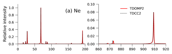
(a)

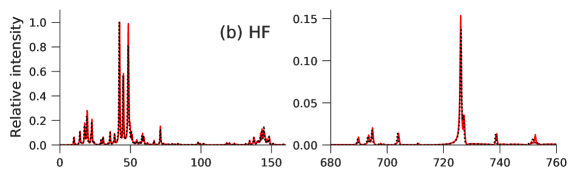
(b)

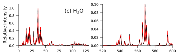
(c)

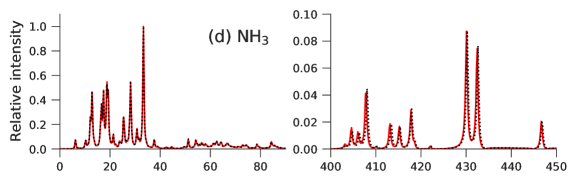
(d)

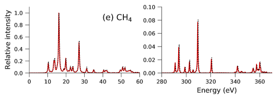
(e)

Figure 1: Absorption spectra computed with TDOMP2 and TDCC2 for Ne, HF, H2O, NH3 and CH4.

Although deviations between the TDOMP2 and TDCC2 spectra are visible, the two methods yield very similar results both in the valence region and in the core region. The excitation energies identified from the simulated spectra by automated peak detection are reported in Table LABEL:lowest_transition_freq for the dipole-allowed states below $30\,\text{eV}$ and confirm the close agreement of TDOMP2 and TDCC2 theory.

Table 1: Dipole-allowed excitation energies (in eV) below $30\,\text{eV}$ extracted from TDOMP2 and TDCC2 simulations.

	TDOMP2	TDCC2		TDOMP2	TDCC2		TDOMP2	TDCC2
H2O	$7.17$	$7.17$	NH3	$6.15$	$6.15$	CH4	$10.25$	$10.42$
	$9.56$	$9.56$		$7.52$	$7.69$		$11.61$	$11.61$
	$11.10$	$11.10$		$10.25$	$10.25$		$13.32$	$13.49$
	$13.66$	$13.66$		$12.13$	$12.13$		$13.66$	$13.83$
	$15.20$	$15.20$		$12.81$	$12.81$		$16.06$	$16.23$
	$18.45$	$18.28$		$16.57$	$16.57$		$18.79$	$18.79$
	$20.15$	$19.81$		$17.42$	$17.42$		$19.81$	$19.81$
	$21.69$	$21.52$		$18.79$	$18.79$		$21.35$	$21.35$
	$23.91$	$23.74$		$19.30$	$19.13$		$22.38$	$22.38$
	$27.33$	$27.33$		$21.35$	$21.35$		$23.57$	$23.74$
	$28.18$	$28.01$		$22.20$	$22.20$		$26.99$	$27.16$
Ne	$16.06$	$15.88$		$23.91$	$23.91$	HF	$10.08$	$9.91$
	$23.06$	$22.89$		$25.45$	$25.28$		$14.35$	$14.18$
	$27.84$	$27.50$		$26.82$	$26.82$		$19.30$	$18.96$
				$28.18$	$28.18$		$22.72$	$22.54$
				$29.21$	$29.21$		$24.25$	$24.08$
							$29.21$	$29.04$

The greatest deviations are found for the HF molecule, especially for the intensities. Some intensity deviations are expected, as the TDOMP2 method is gauge invariant (in the complete basis set limit) while TDCC2 theory is not ^{37, 38}, which is bound to influence transition moments but not necessarily excitation energies. In the core regions, we note that the spectra of H2O, NH3, and CH4 agree qualitatively with the core spectra obtained by Park et al. ²⁴ from TD-EOM-CCSD theory. Keeping in mind that the large deviations between LRCC2/LRCCSD and experimental core excitation energies are ascribed to missing orbital-relaxation effects, it is intriguing to observe that the fully bivariational orbital evolution included in TDOMP2 theory hardly affects the core spectra relative to TDCC2 theory. Using automated peak detection, we find that the differences in excitation energies in the core region between the TDOMP2 and TDCC2 spectra are within $1$–$2$ times the spectral resolution. Since the error of LRCC2 core excitation energies typically is several eV, we conclude that the orbital relaxation provided by TDOMP2 theory is not sufficient to significantly improve the agreement with experimental results. This observation calls for further investigations with larger basis sets, higher resolution (longer simulation times), and full inclusion of double excitations (the TDOCCD and TDNOCCD methods).

3.2 Polarizabilities and first hyperpolarizabilities

Polarizabilities and first hyperpolarizabilities are computed using an electric field given by Eq. (80). After the initial one-cycle ramp we propagate for three optical cycles. The first- and second-order time-dependent dipole response functions are computed by finite difference according to Eqs. (77) and (78), with the first optical cycle of the time evolution discarded because of the ramping. We then perform least-squares fitting ⁶² of the time-domain dipole response functions to the form of Eqs. (75) and (76), obtaining frequency-dependent polarizabilities and hyperpolarizabilities. For all systems we use the field strengths $\mathcal{E}_{0}=\pm 0.0001,\pm 0.0002\,\text{a.u.}$ to compute the dipole derivatives using finite difference.

The diagonal elements of the frequency-dependent polarizability tensor extracted from TDCCSD, TDOMP2, TDCC2, and TDCC2-b simulations for Ne, HF, H2O, NH3, and CH4 are listed in Table 2 along with results from LRCCSD and LRCC2 theory.

Table 2: Polarizabilities (a.u.) of Ne, HF, H2O, NH3, and CH4 extracted from TDCCSD, TDOMP2, TDCC2, and TDCC2-b simulations. The LRCCSD and LRCC2 results for Ne and HF are from Ref. 50 and the remaining LRCCSD and LRCC2 results are computed with the Dalton quantum chemistry program (Ref. 57).

Ne	$\omega\,(\text{a.u.})$	$0.1$	$0.2$	$0.3$	$0.4$	$0.5$
	LRCCSD	$2.74$	$2.83$	$3.01$	$3.38$	$4.23$
	TDCCSD	$2.74$	$2.83$	$3.03$	$3.49$	$4.76$
	TDOMP2	$2.77$	$2.87$	$3.07$	$3.58$	$4.99$
	LRCC2	$2.86$	$2.96$	$3.18$	$3.59$	$4.74$
	TDCC2	$2.87$	$2.98$	$3.19$	$3.75$	$5.29$
	TDCC2-b	$2.86$	$2.97$	$3.18$	$3.73$	$5.26$
HF	$\omega\,(\text{a.u.})$	$0.1$		$0.2$		$0.3$
		$\alpha_{yy}$	$\alpha_{zz}$	$\alpha_{yy}$	$\alpha_{zz}$	$\alpha_{yy}$	$\alpha_{zz}$
	LRCCSD	$4.44$	$6.41$	$4.83$	$6.83$	$6.19$	$7.73$
	TDCCSD	$4.45$	$6.41$	$4.84$	$6.83$	$6.72$	$7.84$
	TDOMP2	$4.56$	$6.49$	$5.03$	$6.94$	$7.71$	$7.96$
	LRCC2	$4.70$	$6.78$	$5.20$	$7.25$	$7.24$	$8.29$
	TDCC2	$4.75$	$6.85$	$5.28$	$7.36$	$8.54$	$8.45$
	TDCC2-b	$4.72$	$6.79$	$5.24$	$7.28$	$8.42$	$8.36$
H2O	$\omega\,(\text{a.u.})$	$0.0428$			$0.0656$			$0.1$
		$\alpha_{xx}$	$\alpha_{yy}$	$\alpha_{zz}$	$\alpha_{xx}$	$\alpha_{yy}$	$\alpha_{zz}$	$\alpha_{xx}$	$\alpha_{yy}$	$\alpha_{zz}$
	LRCCSD	$8.78$	$9.93$	$9.11$	$8.89$	$9.99$	$9.19$	$9.18$	$10.14$	$9.37$
	TDCCSD	$8.78$	$9.93$	$9.11$	$8.90$	$10.00$	$9.19$	$9.19$	$10.14$	$9.37$
	TDOMP2	$9.16$	$10.06$	$9.34$	$9.29$	$10.13$	$9.42$	$9.62$	$10.27$	$9.63$
	LRCC2	$9.41$	$10.43$	$9.63$	$9.55$	$10.50$	$9.71$	$9.91$	$10.66$	$9.92$
	TDCC2	$9.51$	$10.56$	$9.74$	$9.65$	$10.63$	$9.83$	$10.01$	$10.79$	$10.06$
	TDCC2-b	$9.44$	$10.47$	$9.66$	$9.58$	$10.54$	$9.74$	$9.94$	$10.71$	$9.97$
NH3	$\omega\,(\text{a.u.})$	$0.0428$		$0.0656$		$0.1$
		$\alpha_{yy}$	$\alpha_{zz}$	$\alpha_{yy}$	$\alpha_{zz}$	$\alpha_{yy}$	$\alpha_{zz}$
	LRCCSD	$13.10$	$15.04$	$13.20$	$15.35$	$13.44$	$16.15$
	TDCCSD	$13.10$	$15.05$	$13.20$	$15.36$	$13.45$	$16.15$
	TDOMP2	$13.23$	$15.60$	$13.34$	$15.98$	$13.59$	$16.95$
	LRCC2	$13.56$	$15.86$	$13.67$	$16.21$	$13.92$	$17.15$
	TDCC2	$13.72$	$16.03$	$13.83$	$16.43$	$14.10$	$17.40$
	TDCC2-b	$13.64$	$15.93$	$13.75$	$16.32$	$14.01$	$17.28$
CH4	$\omega\,(\text{a.u.})$	$0.0656$	$0.1$	$0.2$
	LRCCSD	$17.05$	$17.39$	$19.55$
	TDCCSD	$17.05$	$17.39$	$19.58$
	TDOMP2	$17.18$	$17.53$	$19.79$
	LRCC2	$17.49$	$17.84$	$20.08$
	TDCC2	$17.69$	$18.05$	$20.34$
	TDCC2-b	$17.61$	$17.96$	$20.25$

All three diagonal elements are identical by symmetry for Ne and CH4, $\alpha_{xx}=\alpha_{yy}$ for HF and NH3, and off-diagonal elements vanish for all systems considered here. The polarizability diverges at the (dipole-allowed) excitation energies and, therefore, we select frequencies below the first dipole-allowed transition in Table LABEL:lowest_transition_freq (roughly $0.6\,\text{a.u.}$ for Ne, $0.4\,\text{a.u.}$ for HF, $0.3\,\text{a.u.}$ for H2O, $0.2\,\text{a.u.}$ for NH3, and $0.4\,\text{a.u.}$ for CH4).

The benchmark study by Larsen et al. ⁵⁰ indicated that LRCCSD theory yields accurate static and dynamic polarizabilities, although triple excitations are needed to obtain results very close to FCI theory, whereas results from LRCC2 theory are significantly less accurate. Our results in Table 2 confirm this finding in the sense that TDCC2 (and LRCC2) results are quite far from the corresponding TDCCSD (and LRCCSD) results. We also note that TDCCSD and LRCCSD results agree to a much greater extent than the results from TDCC2 and LRCC2 theory.

Unfortunately, we have not been able to identify the source of this behavior of the TDCC2 model. The agreement between the results from simulations and from response theory generally worsen as the frequency approaches the lowest-lying dipole-allowed transition. In this “semi-transparent” regime, the assumptions of linear response theory are violated and the first-order time-dependent induced dipole moment can not be described as the simple function in Eq. (75).

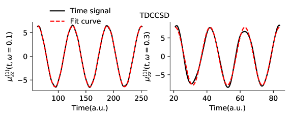
(a)

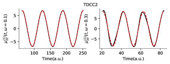
(b)

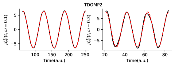
(c)

Figure 2: The zz-component of the first-order dipole responses for HF at $\omega=0.1\,\text{a.u.}$ and $\omega=0.3\,\text{a.u.}$ from TDCCSD, TDCC2, and TDOMP2 simulations.

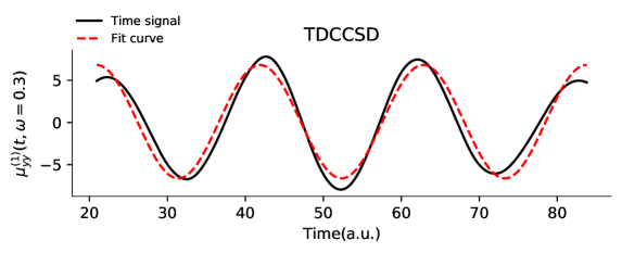
(a)

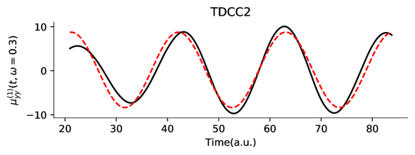
(b)

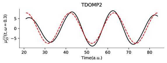
(c)

Figure 3: The yy-component of the first-order dipole responses for HF at $\omega=0.3\,\text{a.u.}$ from TDCCSD, TDCC2, and TDOMP2 simulations.

This is confirmed by the plots of simulated time signals and the least-squares fits in Fig. 2 where the former clearly can only be accurately described by Eq. (75) at sufficiently low (transparent) frequencies. The TDCC2 least-squares fits, however, do not appear worse than those of TDCCSD or TDOMP2 theory. Hence, larger deviations from the form in Eq. (75) can not explain the discrepancies between TDCC2 and LRCC2 results.

Furthermore, we note the relatively large discrepancy between the LRCCSD and TDCCSD results for the HF molecule at $\omega=0.3$ a.u. and the Ne atom at $\omega=0.4$ a.u. and $\omega=0.5$ a.u. In these cases the first-order response function extracted from the time-dependent simulations (77) for all methods considered does not agree with the assumption of a pure cosine wave (75), as shown in Fig. 3 for the HF molecule. The source of deviation is a combined effect of proximity to a pole, non-adiabatic effects arising from ramping up the field over a single cycle, and the absence of higher-order corrections in the finite-difference expressions for the response functions ⁴⁹. This is also likely to be the source of the irregular behavior of $\alpha_{yy}$ computed with the TDCC2 and TDCC2-b methods.

Interestingly, we observe that polarizabilities from TDOMP2 theory are generally in better agreement with the TDCCSD values than those from TDCC2 (and LRCC2) theory. This trend is particularly evident from Fig. 4 where we have plotted the dispersion of the isotropic polarizability, $\alpha_{\text{iso}}=(\alpha_{xx}+\alpha_{yy}+\alpha_{zz})/3$.

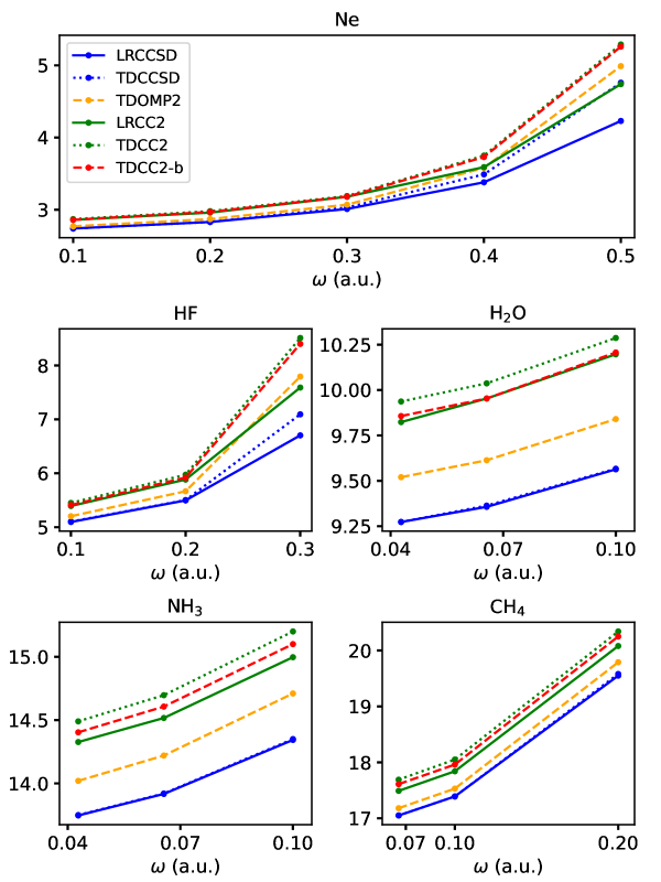
Figure 4: Isotropic polarizabilities extracted from TDCC2, TDCC2-b, TDOMP2, and TDCCSD simulations, and from LRCC2 and LRCCSD calculations.

Keeping in mind the similarity between the TDOMP2 and TDCC2 spectra, the pronounced difference between TDOMP2 and TDCC2 polarizabilities is somewhat surprising. It is, however, in agreement with the observation by Larsen et al. ⁵⁰ that orbital relaxation has a sizeable impact on polarizabilities within CC theory, albeit not always improving the results relative to FCI calculations. Only static polarizabilities were considered by Larsen et al. ⁵⁰ since the orbital relaxation—formulated as a variational HF constraint within conventional CC response theory—leads to spurious uncorrelated poles in the response functions, making it useless for dynamic polarizabilities. The orbitals are treated as fully bivariational variables within TDOMP2 theory and, consequently, spurious poles are avoided. ³⁷ Our results, therefore, seem to indicate that a fully bivariational treatment of orbital relaxation is beneficial for polarizability predictions.

The partial orbital relaxation included in the TDCC2-b method does not yield equally good polarizabilities. In most cases, the results are nearly identical to the TDCC2 ones, except for the H2O and NH3 molecules where the TCCC2-b polarizabilities are closer to the LRCC2 results, see Fig. 4.

In Table 3 we list frequency-dependent first hyperpolarizabilities for HF, H2O, and NH3. Only the nonvanishing diagonal components of the practically most important response tensors corresponding to optical rectification (OR), $\beta^{\text{OR}}_{iii}=\beta_{iii}(0,\omega,-\omega)$, and second harmonic generation (SHG), $\beta^{\text{SHG}}_{iii}=\beta_{iii}(-2\omega,\omega,\omega)$, are computed. Formally expressable as a double summation over all excited states, the first hyperpolarizability generally requires a high-level description of electron correlation effects for accurate calculations ⁶³. This is reflected in our results by the relatively large difference between the TDCC2 and TDCCSD methods.

Table 3: First hyperpolarizabilities (a.u.) of HF, H2O, and NH3 from TDCCSD, TDOMP2, TDCC2, and TDCC2-b simulations. Notation: $\beta_{iii}^{\text{OR}}=\beta_{iii}(0;\omega,-\omega)$ and $\beta_{iii}^{\text{SHG}}=\beta_{iii}(-2\omega;\omega,\omega)$. The LRCCSD and LRCC2 results for HF are taken from Larsen et al. ⁵⁰

HF	$\omega\,(\text{a.u.})$	$0.1$		$0.2$		$0.3$
		$\beta_{zzz}^{\text{OR}}$	$\beta_{zzz}^{\text{SHG}}$	$\beta_{zzz}^{\text{OR}}$	$\beta_{zzz}^{\text{SHG}}$	$\beta_{zzz}^{\text{OR}}$	$\beta_{zzz}^{\text{SHG}}$
	LRCCSD	$12.81$	$14.38$	$15.28$	$29.40$	$21.86$	$-229.70$
	TDCCSD	$12.89$	$14.45$	$15.63$	$29.32$	$25.11$	$-73.94$
	TDOMP2	$13.05$	$14.66$	$15.21$	$28.16$	$24.98$	$-65.73$
	LRCC2	$15.52$	$17.52$	$18.69$	$37.67$	$27.35$	$-51.78$
	TDCC2	$16.53$	$18.63$	$19.40$	$36.39$	$32.11$	$-61.17$
	TDCC2-b	$15.32$	$17.26$	$17.95$	$33.56$	$29.76$	$-64.95$
H2O	$\omega\,(\text{a.u.})$	$0.0428$		$0.0656$		$0.1$
		$\beta_{zzz}^{\text{OR}}$	$\beta_{zzz}^{\text{SHG}}$	$\beta_{zzz}^{\text{OR}}$	$\beta_{zzz}^{\text{SHG}}$	$\beta_{zzz}^{\text{OR}}$	$\beta_{zzz}^{\text{SHG}}$
	LRCCSD	$-9.11$	$-9.59$	$-9.43$	$-10.72$	$-10.25$	$-14.52$
	TDCCSD	$-9.14$	$-9.62$	$-9.50$	$-10.78$	$-10.47$	$-14.69$
	TDOMP2	$-9.92$	$-10.49$	$-10.33$	$-11.80$	$-11.57$	$-17.63$
	LRCC2	$-12.39$	$-13.12$	$-12.87$	$-14.83$	$-14.11$	$-20.76$
	TDCC2	$-13.63$	$-14.42$	$-14.17$	$-16.18$	$-15.75$	$-23.70$
	TDCC2-b	$-11.89$	$-12.58$	$-12.38$	$-14.15$	$-13.84$	$-21.01$
NH3	$\omega\,(\text{a.u.})$	$0.0428$				$0.0656$
		$\beta_{yyy}^{\text{OR}}$	$\beta_{yyy}^{\text{SHG}}$	$\beta_{zzz}^{\text{OR}}$	$\beta_{zzz}^{\text{SHG}}$	$\beta_{yyy}^{\text{OR}}$	$\beta_{yyy}^{\text{SHG}}$	$\beta_{zzz}^{\text{OR}}$	$\beta_{zzz}^{\text{SHG}}$
	LRCCSD	$-14.90$	$-15.50$	$23.90$	$28.02$	$-15.30$	$-16.88$	$26.57$	$40.49$
	TDCCSD	$-14.94$	$-15.59$	$24.20$	$28.45$	$-15.47$	$-17.27$	$27.35$	$41.94$
	TDOMP2	$-15.64$	$-16.42$	$30.66$	$36.26$	$-15.81$	$-17.39$	$35.50$	$58.38$
	LRCC2	$-16.69$	$-17.40$	$33.80$	$39.87$	$-17.16$	$-19.01$	$37.72$	$58.61$
	TDCC2	$-17.32$	$-18.13$	$35.80$	$41.90$	$-17.51$	$-19.17$	$41.24$	$66.61$
	TDCC2-b	$-17.00$	$-17.79$	$32.60$	$38.26$	$-17.19$	$-18.81$	$37.80$	$61.67$

While $\beta^{\text{OR}}_{iii}$ is singular when the magnitude of the radiation frequency $\omega$ equals an excitation energy of the molecule, $\beta^{\text{SHG}}_{iii}$ has an additional set of poles at half the excitation energies. The $\beta^{\text{SHG}}_{zzz}$ results at $\omega=0.3\,\text{a.u.}$ for the HF molecule in Table 3 are past the first pole and, hence, the sign has changed compared with the SHG results at lower frequencies. The large negative value of $\beta^{\text{SHG}}_{zzz}$ at $\omega=0.3\,\text{a.u.}$ obtained with the LRCCSD method for the HF molecule is due to proximity to two dipole-allowed, $z$-polarized excitations at $0.598\,\text{a.u.}$ (oscillator strength $0.005$) and at $0.532\,\text{a.u.}$ (oscillator strength $0.157$).

The agreement between real-time simulations and response theory is seen to be somewhat worse than for polarizabilities, especially for frequencies closer to a pole of the hyperpolarizability. This can to a large extent be ascribed to the second-order dipole response extracted from the time-dependent simulations not being well described by the sinusoidal form of Eq. (76), as illustrated in Fig. 5.

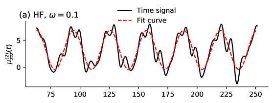
(a)

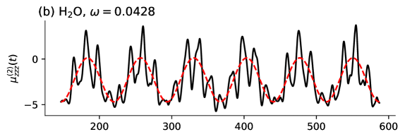
(b)

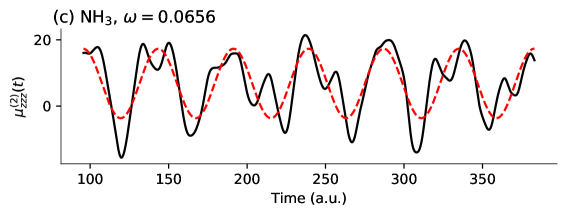
(c)

Figure 5: Second-order dipole responses for HF, H2O, and NH3 from TDCCSD simulations.

Analogous observations were done by Ding et al. ⁴⁹ in the context of real-time time-dependent density-functional theory simulations. Hence, moving on to higher-order nonlinear optical properties can not generally be expected to provide more than a rough estimate with the present extraction algorithm.

As for the polarizabilites above, we observe that first hyperpolarizabilities obtained from TDOMP2 simulations are generally closer to TDCCSD and LRCCSD results than those from TDCC2 and LRCC2 theory. The source of the improvement over TDCC2 theory must be the bivariational orbital relaxation, although we stress that the larger differences between TDOMP2 theory and TDCCSD theory, which are particularly pronounced for NH3, clearly demonstrate the insufficient electron-correlation treatment of the former for highly accurate predictions of nonlinear optical properties. The importance of orbital relaxation is corroborated by the TDCC2-b hyperpolarizabilities, which are somewhat closer to the TDOMP2 and TDCCSD results than the TDCC2 ones.

4 Concluding remarks

In this work we have presented a new unified derivation of TDOCC and TDNOCC theories, including the second-order approximations TDOMP2 and TDNOMP2, using exponential orbital-rotation operators and the bivariational Euler-Lagrange equations. Using five small 10-electron molecules as test cases, we have extracted absorption spectra and frequency-dependent polarizabilities and hyperpolarizabilities from TDOMP2 simulations with weak fields within the electric-dipole approximation and compared the results with those from conventional TDCCSD and TDCC2 simulations. While the TDOMP2 absorption spectra are almost identical to TDCC2 spectra, including in the spectral region of core excitations, the TDOMP2 polarizabilities and hyperpolarizabilities are significantly closer to TDCCSD results than those from TDCC2 simulations, especially for frequencies comfortably away from resonances. Further corroborated by TDCC2-b simulations, our results strongly indicate that fully (bi-)variational orbital relaxation is important for frequency-dependent polarizabilities and hyperpolarizabilities, whilst nearly irrelevant for absorption spectra.

Combined with the observations by Pathak et al. ²⁶, who found that TDOMP2 theory outperforms TDCC2 theory for strong-field many-electron dynamics, our results may serve as a motivation for further development of TDOMP2 theory. First of all, a reduced-scaling implementation of TDOMP2 theory, obtained, for example, by exploiting sparsity of the correlating doubles amplitudes, ⁶⁴ can provide reasonably accurate results for larger systems and basis sets that are out of reach for today’s TDCC implementations. Second, an efficient implementation of OMP2 linear and quadratic response functions is warranted.

This work was supported by the Research Council of Norway through its Centres of Excellence scheme, project number 262695, by the European Research Council under the European Union Seventh Framework Program through the Starting Grant BIVAQUM, ERC-STG-2014 grant agreement No. 639508, and by the Norwegian Supercomputing Program (NOTUR) through a grant of computer time (Grant No. NN4654K). SK and TBP acknowledge the support of the Centre for Advanced Study in Oslo, Norway, which funded and hosted our CAS research project Attosecond Quantum Dynamics Beyond the Born-Oppenheimer Approximation during the academic year of 2021/2022. We thank Prof. Sonia Coriani for helpful discussions and for providing the Lanczos-driven LRCC2 results reported in the Supporting Information, and Mr. Sindre Bjøringsøy Johnsen for making the cover art.

Algebraic expressions for the closed-shell spin-restricted OMP2 method, molecular geometries, electronic ground-state energies and electric-dipole moments, and comparison of TDCC2 absorption spectra with those from LRCC2 theory in the range $0$–$930\,\text{eV}$. This information is available free of charge via the Internet at https://pubs.acs.org.

References

- Olsen and Jørgensen 1985 Olsen, J.; Jørgensen, P. Linear and nonlinear response functions for an exact state and for an MCSCF state. J. Chem. Phys. 1985, 82, 3235–3264
- Li et al. 2020 Li, X.; Govind, N.; Isborn, C.; DePrince, A. E.; Lopata, K. Real-Time Time-Dependent Electronic Structure Theory. Chem. Rev. 2020, 120, 9951–9993
- Runge and Gross 1984 Runge, E.; Gross, E. K. Density-functional theory for time-dependent systems. Phys. Rev. Lett. 1984, 52, 997–1000
- van Leeuwen 1999 van Leeuwen, R. Mapping from densities to potentials in time-dependent density-functional theory. Phys. Rev. Lett. 1999, 82, 3863–3866
- Ullrich 2012 Ullrich, C. A. Time-Dependent Density-Functional Theory; Oxford University Press: Oxford, 2012
- Zanghellini et al. 2003 Zanghellini, J.; Kitzler, M.; Fabian, C.; Brabec, T.; Scrinzi, A. An MCTDHF Approach to Multielectron Dynamics in Laser Fields. Laser Phys. 2003, 13, 1064–1068
- Kato and Kono 2004 Kato, T.; Kono, H. Time-dependent multiconfiguration theory for electronic dynamics of molecules in an intense laser field. Chem. Phys. Lett. 2004, 392, 533–540
- Meyer et al. 2009 Meyer, H.-D., Gatti, F., Worth, G., Eds. Multidimensional Quantum Dynamics: MCTDH Theory and Applications; Wiley: Weinheim, Germany, 2009
- Hochstuhl et al. 2014 Hochstuhl, D.; Hinz, C. M.; Bonitz, M. Time-dependent multiconfiguration methods for the numerical simulation of photoionization processes of many-electron atoms. Eur. Phys. J. Spec. Top. 2014, 223, 177–336
- Sato and Ishikawa 2013 Sato, T.; Ishikawa, K. L. Time-dependent complete-active-space self-consistent-field method for multielectron dynamics in intense laser fields. Phys. Rev. A 2013, 88, 023402
- Miyagi and Madsen 2013 Miyagi, H.; Madsen, L. B. Time-dependent restricted-active-space self-consistent-field theory for laser-driven many-electron dynamics. Phys. Rev. A 2013, 87, 062511
- Bauch et al. 2014 Bauch, S.; Sørensen, L. K.; Madsen, L. B. Time-dependent generalized-active-space configuration-interaction approach to photoionization dynamics of atoms and molecules. Phys. Rev. A 2014, 90, 062508
- Bartlett and Musial 2007 Bartlett, R.; Musial, M. Coupled-cluster theory in quantum chemistry. Rev. Mod. Phys. 2007, 79, 291–352
- Krylov 2008 Krylov, A. I. Equation-of-Motion Coupled-Cluster Methods for Open-Shell and Electronically Excited Species: The Hitchhiker’s Guide to Fock Space. Annu. Rev. Phys. Chem. 2008, 59, 433–462
- Bartlett 2012 Bartlett, R. J. Coupled-cluster theory and its equation-of-motion extensions. Wiley Interdiscip. Rev. Comput. Mol. Sci. 2012, 2, 126–138
- Huber and Klamroth 2011 Huber, C.; Klamroth, T. Explicitly time-dependent coupled cluster singles doubles calculations of laser-driven many-electron dynamics. J. Chem. Phys. 2011, 134, 054113
- Kvaal 2012 Kvaal, S. Ab initio quantum dynamics using coupled-cluster. J. Chem. Phys. 2012, 136, 194109
- Nascimento and DePrince 2016 Nascimento, D. R.; DePrince, A. E. Linear Absorption Spectra from Explicitly Time-Dependent Equation-of-Motion Coupled-Cluster Theory. J. Chem. Theory Comput. 2016, 12, 5834–5840
- Nascimento and DePrince 2017 Nascimento, D. R.; DePrince, A. E. Simulation of Near-Edge X-ray Absorption Fine Structure with Time-Dependent Equation-of-Motion Coupled-Cluster Theory. J. Phys. Chem. Lett. 2017, 8, 2951–2957
- Sato et al. 2018 Sato, T.; Pathak, H.; Orimo, Y.; Ishikawa, K. L. Time-dependent optimized coupled-cluster method for multielectron dynamics. J. Chem. Phys. 2018, 148, 051101
- Pedersen and Kvaal 2019 Pedersen, T. B.; Kvaal, S. Symplectic integration and physical interpretation of time-dependent coupled-cluster theory. J. Chem. Phys. 2019, 150, 144106
- Nascimento and DePrince 2019 Nascimento, D. R.; DePrince, A. E. A general time-domain formulation of equation-of-motion coupled-cluster theory for linear spectroscopy. J. Chem. Phys. 2019, 151, 204107
- Koulias et al. 2019 Koulias, L. N.; Williams-Young, D. B.; Nascimento, D. R.; Deprince, A. E.; Li, X. Relativistic Real-Time Time-Dependent Equation-of-Motion Coupled-Cluster. J. Chem. Theory Comput. 2019, 15, 6617–6624
- Park et al. 2019 Park, Y. C.; Perera, A.; Bartlett, R. J. Equation of motion coupled-cluster for core excitation spectra: Two complementary approaches. J. Chem. Phys. 2019, 151, 164117
- Pathak et al. 2020 Pathak, H.; Sato, T.; Ishikawa, K. L. Time-dependent optimized coupled-cluster method for multielectron dynamics. II. A coupled electron-pair approximation. J. Chem. Phys. 2020, 152, 124115
- Pathak et al. 2020 Pathak, H.; Sato, T.; Ishikawa, K. L. Time-dependent optimized coupled-cluster method for multielectron dynamics. III. A second-order many-body perturbation approximation. J. Chem. Phys. 2020, 153, 034110
- Pathak et al. 2020 Pathak, H.; Sato, T.; Ishikawa, K. L. Study of laser-driven multielectron dynamics of Ne atom using time-dependent optimised second-order many-body perturbation theory. Mol. Phys. 2020, 118, e1813910
- Skeidsvoll et al. 2020 Skeidsvoll, A. S.; Balbi, A.; Koch, H. Time-dependent coupled-cluster theory for ultrafast transient-absorption spectroscopy. Phys. Rev. A 2020, 102, 023115
- Kristiansen et al. 2020 Kristiansen, H. E.; Schøyen, Ø. S.; Kvaal, S.; Pedersen, T. B. Numerical stability of time-dependent coupled-cluster methods for many-electron dynamics in intense laser pulses. J. Chem. Phys. 2020, 152, 071102
- Pedersen et al. 2021 Pedersen, T. B.; Kristiansen, H. E.; Bodenstein, T.; Kvaal, S.; Schøyen, Ø. S. Interpretation of coupled-cluster many-electron dynamics in terms of stationary states. J. Chem. Theory Comput. 2021, 17, 388–404
- Cooper et al. 2021 Cooper, B. C.; Koulias, L. N.; Nascimento, D. R.; Li, X.; DePrince, A. E. Short Iterative Lanczos Integration in Time-Dependent Equation-of-Motion Coupled-Cluster Theory. J. Phys. Chem. A 2021, 125, 5438–5447
- Park et al. 2021 Park, Y. C.; Perera, A.; Bartlett, R. J. Equation of motion coupled-cluster study of core excitation spectra II: Beyond the dipole approximation. J. Chem. Phys. 2021, 155
- Skeidsvoll et al. 2022 Skeidsvoll, A. S.; Moitra, T.; Balbi, A.; Paul, A. C.; Coriani, S.; Koch, H. Simulating weak-field attosecond processes with a Lanczos reduced basis approach to time-dependent equation-of-motion coupled-cluster theory. Phys. Rev. A 2022, 105, 023103
- Hoodbhoy and Negele 1978 Hoodbhoy, P.; Negele, J. W. Time-dependent coupled-cluster approximation to nuclear dynamics. I. Application to a solvable model. Phys. Rev. C 1978, 18, 2380–2394
- Koch and Jørgensen 1990 Koch, H.; Jørgensen, P. Coupled cluster response functions. J. Chem. Phys. 1990, 93, 3333–3344
- Pedersen and Koch 1997 Pedersen, T. B.; Koch, H. Coupled cluster response functions revisited. J. Chem. Phys. 1997, 106, 8059–8072
- Pedersen et al. 1999 Pedersen, T. B.; Koch, H.; Hättig, C. Gauge invariant coupled cluster response theory. J. Chem. Phys. 1999, 110, 8318–8327
- Pedersen et al. 2001 Pedersen, T. B.; Fernández, B.; Koch, H. Gauge invariant coupled cluster response theory using optimized nonorthogonal orbitals. J. Chem. Phys. 2001, 114, 6983–6993
- Sherrill et al. 1998 Sherrill, C. D.; Krylov, A. I.; Byrd, E. F. C.; Head-Gordon, M. Energies and analytic gradients for a coupled-cluster doubles model using variational Brueckner orbitals: Application to symmetry breaking in \chO4+. J. Chem. Phys. 1998, 109, 4171–4181
- Krylov et al. 1998 Krylov, A. I.; Sherrill, C. D.; Byrd, E. F.; Head-Gordon, M. Size-consistent wave functions for nondynamical correlation energy: The valence active space optimized orbital coupled-cluster doubles model. J. Chem. Phys. 1998, 109, 10669–10678
- Köhn and Olsen 2005 Köhn, A.; Olsen, J. Orbital-optimized coupled-cluster theory does not reproduce the full configuration-interaction limit. J. Chem. Phys. 2005, 122, 084116
- Myhre 2018 Myhre, R. H. Demonstrating that the nonorthogonal orbital optimized coupled cluster model converges to full configuration interaction. J. Chem. Phys. 2018, 148, 094110
- Bozkaya et al. 2011 Bozkaya, U.; Turney, J. M.; Yamaguchi, Y.; Schaefer, H. F.; Sherrill, C. D. Quadratically convergent algorithm for orbital optimization in the orbital-optimized coupled-cluster doubles method and in orbital-optimized second-order Møller-Plesset perturbation theory. J. Chem. Phys. 2011, 135, 104103
- Arponen 1983 Arponen, J. Variational principles and linked-cluster exp S expansions for static and dynamic many-body problems. Ann. Phys. 1983, 151, 311–382
- Christiansen et al. 1995 Christiansen, O.; Koch, H.; Jørgensen, P. The second-order approximate coupled cluster singles and doubles model CC2. Chem. Phys. Lett. 1995, 243, 409–418
- Kats et al. 2006 Kats, D.; Korona, T.; Schütz, M. Local CC2 electronic excitation energies for large molecules with density fitting. J. Chem. Phys. 2006, 125, 104106
- Repisky et al. 2015 Repisky, M.; Konecny, L.; Kadek, M.; Komorovsky, S.; Malkin, O. L.; Malkin, V. G.; Ruud, K. Excitation Energies from Real-Time Propagation of the Four-Component Dirac–Kohn–Sham Equation. J. Chem. Theory Comput. 2015, 11, 980–991
- Goings and Li 2016 Goings, J. J.; Li, X. An atomic orbital based real-time time-dependent density functional theory for computing electronic circular dichroism band spectra. J. Chem. Phys. 2016, 144, 234102
- Ding et al. 2013 Ding, F.; Van Kuiken, B. E.; Eichinger, B. E.; Li, X. An efficient method for calculating dynamical hyperpolarizabilities using real-time time-dependent density functional theory. J. Chem. Phys. 2013, 138, 064104
- Larsen et al. 1999 Larsen, H.; Olsen, J.; Hättig, C.; Jørgensen, P.; Christiansen, O.; Gauss, J. Polarizabilities and first hyperpolarizabilities of HF, Ne, and BH from full configuration interaction and coupled cluster calculations. J. Chem. Phys. 1999, 111, 1917–1925
- Dunning, Jr. 1989 Dunning, Jr., T. H. Gaussian basis sets for use in correlated molecular calculations. I. The atoms boron through neon and hydrogen. J. Chem. Phys. 1989, 90, 1007–1023
- Kendall et al. 1992 Kendall, R. A.; Dunning, Jr., T. H.; Harrison, R. J. Electron affinities of the first-row atoms revisited. Systematic basis sets and wave functions. J. Chem. Phys. 1992, 96, 6796–7006
- Woon and Dunning, Jr. 1994 Woon, D. E.; Dunning, Jr., T. H. Gaussian basis sets for use in correlated calculations. IV. Calculation of static electrical response properties. J. Chem. Phys. 1994, 100, 2975–2988
- Pritchard et al. 2019 Pritchard, B. P.; Altarawy, D.; Didier, B.; Gibson, T. D.; Windus, T. L. New Basis Set Exchange: An Open, Up-to-Date Resource for the Molecular Sciences Community. J. Chem. Inf. Model. 2019, 59, 4814–4820
- Sun et al. 2018 Sun, Q.; Berkelbach, T. C.; Blunt, N. S.; Booth, G. H.; Guo, S.; Li, Z.; Liu, J.; McClain, J. D.; Sayfutyarova, E. R.; Sharma, S.; Wouters, S.; Chan, G. K. L. PySCF: the Python‐based simulations of chemistry framework. Wiley Interdiscip. Rev. Comput. Mol. Sci. 2018, 8, e1340
- Helgaker et al. 2014 Helgaker, T.; Jørgensen, P.; Olsen, J. Molecular electronic-structure theory; John Wiley & Sons, 2014
- Aidas et al. 2014 Aidas, K.; Angeli, C.; Bak, K. L.; Bakken, V.; Bast, R.; Boman, L.; Christiansen, O.; Cimiraglia, R.; Coriani, S.; Dahle, P.; Dalskov, E. K.; Ekström, U.; Enevoldsen, T.; Eriksen, J. J.; Ettenhuber, P.; Fernández, B.; Ferrighi, L.; Fliegl, H.; Frediani, L.; Hald, K.; Halkier, A.; Hättig, C.; Heiberg, H.; Helgaker, T.; Hennum, A. C.; Hettema, H.; Hjertenaes, E.; Høst, S.; Høyvik, I.-M.; Iozzi, M. F.; Jansík, B.; Jensen, H. J. A.; Jonsson, D.; Jørgensen, P.; Kauczor, J.; Kirpekar, S.; Kjaergaard, T.; Klopper, W.; Knecht, S.; Kobayashi, R.; Koch, H.; Kongsted, J.; Krapp, A.; Kristensen, K.; Ligabue, A.; Lutnaes, O. B.; Melo, J. I.; Mikkelsen, K. V.; Myhre, R. H.; Neiss, C.; Nielsen, C. B.; Norman, P.; Olsen, J.; Olsen, J. M. H.; Osted, A.; Packer, M. J.; Pawlowski, F.; Pedersen, T. B.; Provasi, P. F.; Reine, S.; Rinkevicius, Z.; Ruden, T. A.; Ruud, K.; Rybkin, V. V.; Sałek, P.; Samson, C. C. M.; Sánchez de Merás, A.; Saue, T.; Sauer, S. P. A.; Schimmelpfennig, B.; Sneskov, K.; Steindal, A. H.; Sylvester-Hvid, K. O.; Taylor, P. R.; Teale, A. M.; Tellgren, E. I.; Tew, D. P.; Thorvaldsen, A. J.; Thøgersen, L.; Vahtras, O.; Watson, M. A.; Wilson, D. J. D.; Ziolkowski, M.; Ågren, H. The Dalton quantum chemistry program system. Wiley Interdiscip. Rev. Comput. Mol. Sci. 2014, 4, 269–284
- Olsen et al. 2020 Olsen, J. M. H.; Reine, S.; Vahtras, O.; Kjellgren, E.; Reinholdt, P.; Hjorth Dundas, K. O.; Li, X.; Cukras, J.; Ringholm, M.; Hedegård, E. D.; Di Remigio, R.; List, N. H.; Faber, R.; Cabral Tenorio, B. N.; Bast, R.; Pedersen, T. B.; Rinkevicius, Z.; Sauer, S. P. A.; Mikkelsen, K. V.; Kongsted, J.; Coriani, S.; Ruud, K.; Helgaker, T.; Jensen, H. J. A.; Norman, P. Dalton Project: A Python platform for molecular- and electronic-structure simulations of complex systems. J. Chem. Phys. 2020, 152, 214115
- Hairer et al. 2006 Hairer, E.; Lubich, C.; Wanner, G. Geometric Numerical Integration, 2nd ed.; Springer: Berlin, 2006
- Schreiber et al. 2008 Schreiber, M.; Silva-Junior, M. R.; Sauer, S. P. A.; Thiel, W. Benchmarks for electronically excited states: CASPT2, CC2, CCSD, and CC3. J. Chem. Phys. 2008, 128, 134110
- Coriani et al. 2012 Coriani, S.; Christiansen, O.; Fransson, T.; Norman, P. Coupled-cluster response theory for near-edge x-ray-absorption fine structure of atoms and molecules. Phys. Rev. A 2012, 85, 022507
- Hastie et al. 2009 Hastie, T.; Tibshirani, R.; Friedman, J. The Elements of Statistical Learning: Data Mining, Inference, and Prediction; Springer New York: New York, NY, 2009; pp 43–99
- Christiansen et al. 2006 Christiansen, O.; Coriani, S.; Gauss, J.; Hättig, C.; Jørgensen, P.; Pawłowski, F.; Rizzo, A. In Non-Linear Optical Properties of Matter: From Molecules to Condensed Phases; Papadopoulos, M. G., Sadlej, A. J., Leszczynski, J., Eds.; Springer Netherlands: Dordrecht, 2006; Chapter 2, pp 51–99
- Crawford et al. 2019 Crawford, T. D.; Kumar, A.; Bazanté, A. P.; Remigio, R. D. Reduced-scaling coupled cluster response theory: Challenges and opportunities. Wiley Interdiscip. Rev. Comput. Mol. Sci. 2019, 9, e1406