Correction of high-order $L_{k}$ approximation for subdiffusion

Abstract

The subdiffusion equations with a Caputo fractional derivative of order $\alpha\in(0,1)$ arise in a wide variety of practical problems, which is describing the transport processes, in the force-free limit, slower than Brownian diffusion. In this work, we derive the correction schemes of the Lagrange interpolation with degree $k$ ($k\leq 6$) convolution quadrature, called $L_{k}$ approximation, for the subdiffusion, which are easy to implement on variable grids. The key step of designing correction algorithm is to calculate the explicit form of the coefficients of $L_{k}$ approximation by the polylogarithm function or Bose-Einstein integral. To construct a $\tau_{8}$ approximation of Bose-Einstein integral, the desired $(k+1-\alpha)$th-order convergence rate can be proved for the correction $L_{k}$ scheme with nonsmooth data, which is higher than $k$th-order BDF$k$ method in [Jin, Li, and Zhou, SIAM J. Sci. Comput., 39 (2017), A3129–A3152; Shi and Chen, J. Sci. Comput., (2020) 85:28]. The numerical experiments with spectral method are given to illustrate theoretical results.

1 Introduction

The subdiffusion equations are a type of partial differential equations describing the transport processes, which are, in the force-free limit, slower than Brownian diffusion. Many application problems can be modeled by subdiffusion, such as underground environmental problems, transport in turbulent plasma, bacterial motion transport in micelle systems and in heterogeneous rocks, porous systems, dynamics of a bead in a polymeric network Metzler:00 . In this work, we study the high order time discretization schemes by the Lagrange interpolation of degree $k\leq 6$, called $L_{k}$ approximation, for solving the subdiffusion, whose prototype is Podlubny:1999 , for $0<\alpha<1$

$$\left\{\begin{split}&{}^{C}_{0}{D}^{\alpha}_{t}u(t)-Au(t)=f(t),\quad 0<t<T,\\ &u(0)=v.\end{split}\right.$$ (1.1)

Here $f$ is a given function, the operator $A=\Delta$ denotes Laplacian on a polyhedral domain $\Omega\subset\mathbb{R}^{d}$, $d=1,2,3$. The operator ${}^{C}_{0}{D}^{\alpha}_{t}$ denotes the Caputo fractional derivative, namely,

$$^{C}_{0}{D}^{\alpha}_{t}u(t)=\frac{1}{\Gamma(1-\alpha)}\int^{t}_{0}{(t-s)^{-\alpha}u^{\prime}(s)}ds.$$ (1.2)

Because of the nonlocal properties of Caputo fractional derivative (1.2), the correction of higher order $L_{k}$ approximation play a more important role in discretizing Caputo fractional derivatives than classical ones CD:2014 . The striking feature is that higher order $L_{k}$ approximation of nonlocal operators can keep the same computation cost with $L_{1}$ schemes but greatly improve the accuracy. In recent years, there are some important progress has been made for numerically solving the subdiffusion. For example, under the smooth assumption, Lin and Xu developed the $L_{1}$ schemes for the subdiffusion and the optimal convergence rate with $\mathcal{O}(\tau^{2-\alpha})$ has been obtained in LX:2007 . Gao et al. GSZ:2014 showed that the desired $\mathcal{O}(\tau^{3-\alpha})$ convergence rate can be achieved for $L_{2}$ approximation by some numerical simulation. Later on, Lv and Xu establish stability and convergence analysis of $L_{2}$ approximation in LX:2016 . Cao and Li at al. provided a high-order $\mathcal{O}(\tau^{k+1-\alpha})$, $k\leq 5$, for subdiffusion with $L_{k}$ approximation CLC:2015 ; LCL:2016 , where the convergence analysis also remains to be proved.

It is well known that the smoothness of all the data of (1.1) do not imply the smoothness of the solution $u$. For example, the following estimate holds if $f=0$ SY:11 ; SC:2020 , namely,

$$\|^{C}_{0}{D}^{\alpha}_{t}u(t)\|_{L^{2}(\Omega)}\leq ct^{-\alpha}\|u_{0}\|_{L^{2}(\Omega)},$$

which reduces to a parabolic problem $\|\partial_{t}u(t)\|_{L^{2}(\Omega)}\leq ct^{-1}\|u_{0}\|_{L^{2}(\Omega)}$ if $\alpha=1$ (Thomee:2006, , p. 39). It implies that $u$ has an initial layer at $t\rightarrow 0^{+}$ SOG:2017 . In another word, the high-order convergence rates may not hold for nonsmooth data. Hence, the efficiently solving the subdiffusion naturally becomes an urgent topic. Luckily, there are already two predominant discretization techniques in time direction to restore the desired convergence rate for nonsmooth data. The first type is that the nonuniform time meshes/graded meshes are employed to compensate for the singularity of the continuous solution near $t=0$. For example, Stynes et al. capture the singularity of the solution for subdiffusion (1.1) and the optimal convergence rate with $\mathcal{O}(\tau^{2-\alpha})$ of the time discretization schemes can be restored SOG:2017 . The corresponding theoretical and algorithm can also be extended to the Caputo fractional substantial derivative equation CJB:2021 . Using a nonstandard set of basis functions, Kopteva Kopteva:2021 provide an $L_{2}$ approximation for subdiffusion, which proved and restored the optimal order $3-\alpha$ on graded meshes.

The second type is that, based on correction of high-order BDF$k$ or $L_{k}$ approximation, the desired high-order convergence rates can be restored even for nonsmooth initial data. For example, Lubich et al. provided the corrected BDF$2$ and proved the optimal convergence orders for an evolution equaiton with a weakly singular kernels LST:1996 . Jin et al. JLZ:2017 developed correction BDF$k$ ($k\leq 6$) formulas to restore the desired $k$-order convergence rate for subdiffusion (1.1), which also hold for the fractional Feynman-Kac equation with Lévy flight SC:2020 . For $L_{k}$ approximation, Jin et al. JLZ:2016 revisit the error analysis of $L_{1}$ scheme, and establish an $\mathcal{O}(\tau)$ convergence rate for both smooth and nonsmooth initial data. Yan et al. introduced a modified $L_{1}$ scheme for solving (1.1) and obtain optimal convergence rate with $\mathcal{O}(\tau^{2-\alpha})$ for smooth and YKF:2018 . Wang and Yan et al. proved that correction schemes of $L_{2}$ and $L_{3}$ approximations, respectively, have the optimal convergence orders $\mathcal{O}(\tau^{3-\alpha})$ and $\mathcal{O}(\tau^{4-\alpha})$ for both smooth and nonsmooth data WYY:2020 . It seems that there are no published works of high-order $L_{k}$ ($k\geq 4$) approximation with nonsmooth initial data for subdiffusion (1.1). In fact, it is not an easy task for convergence analysis based on the idea of JLZ:2016 ; WYY:2020 ; YKF:2018 , this is due to the complexity of the coefficients in the $L_{k}$ approximation with Bose-Einstein integral. In this work, the key step of designing correction $L_{k}$ schemes is to calculate the explicit form of the coefficients of $L_{k}$ approximation with the polylogarithm function or Bose-Einstein integral BBR:2003 . Moreover, we need to construct the high-order $\tau_{8}$-approximation of order $8$ for Bose-Einstein integral BBR:2003 . Then the desired $(k+1-\alpha)$th-order convergence rate can be proved for the correction $L_{k}$ scheme with nonsmooth data. The main advantage of $L_{k}$ approximation (compared with BDF$k$) is that its convergence rate higher than BDF$k$ method and more easily implemented on variable grids/graded meshes.

The paper is organized as follows. In Section 2, we provide correction of $L_{k}$ approximation at the starting $k$ steps for fractional order evolution equation (1.1). In Section 3, we provide the detailed convergence analysis of correction $L_{k}$ schemes. Some numerical examples are given to show the effectiveness of the presented schemes in Section 4.

2 Correction of high-order $L_{k}$ approximation

Let $V(t)=u(t)-u(0)=u(t)-v$, we can rewrite (1.1) as Podlubny:1999

$$\left\{\begin{split}&{}^{C}_{0}{D}^{\alpha}_{t}V(t)-AV(t)=Av+f(t),\quad 0<t<T,\\ &V(0)=0,\end{split}\right.$$ (2.1)

where we use ${}^{C}_{0}{D}^{\alpha}_{t}u(t)=\partial^{\alpha}_{t}(u(t)-u(0))=\partial^{\alpha}_{t}V(t)=\,^{C}_{0}{D}^{\alpha}_{t}V(t)$ with $V(0)=0$, and $\partial^{\alpha}_{t}$ denotes the left-sided Riemann-Liouville fractional derivative of order $\alpha\in(0,1)$

$$\partial^{\alpha}_{t}u(t)=\frac{1}{\Gamma(1-\alpha)}\frac{\partial}{\partial t}\int^{t}_{0}{(t-s)^{-\alpha}u(s)}ds.$$

2.1 Derivation of the high-order $L_{k}$ approximation

Let $t_{n}=n\tau,n=0,1,\ldots,N,$ be a uniform partition of the time interval $[0,T]$ with the step size $\tau=\frac{T}{N}$, and let $V^{n}$ denote the approximation of $V(t_{n})$ and $f^{n}=f(t_{n})$. Using $k+1$ points $(t_{j-k}$, $V^{j-k})$, $\dots$, $(t_{j-1}$, $V^{j-1})$, $(t_{j},V^{j})$ for $j\geq k$, we can construct the Lagrange interpolation function $L_{k,j}(t)$ of degree $k$ with $k\leq 6$, namely,

$$L_{k,j}[V(t)]=\sum^{k}_{l=0}V^{j-l}\prod^{k}_{i=0,i\neq l}\frac{t-t_{j-i}}{t_{j-l}-t_{j-i}},~{}~{}t\in(t_{j-1},t_{j}),$$ (2.2)

and its derivative is

$$\begin{split}L^{\prime}_{1,j}[V(t)]&=\sum^{k}_{l=0}V^{j-l}\sum^{k}_{m=0,m\neq l}\frac{1}{t_{j-l}-t_{j-m}},~{}~{}k=1;\\ L^{\prime}_{k,j}[V(t)]&=\sum^{k}_{l=0}V^{j-l}\sum^{k}_{m=0,m\neq l}\left(\frac{1}{t_{j-l}-t_{j-m}}\prod^{k}_{i=0,i\neq l,i\neq m}\frac{t-t_{j-i}}{t_{j-l}-t_{j-i}}\right),~{}~{}2\leq k\leq 6.\end{split}$$ (2.3)

Moreover, we take $V^{-1}=V^{-2}=\dots=V^{-k}=0$ and $t_{-1}=-t_{1},t_{-2}=-t_{2},\dots,t_{-k}=-t_{k}$ such that all quantities appearing in (2.2) and (2.3) are defined for $1\leq j\leq k-1$. Then the $L_{k}$ approximation of the Caputo fractional derivative is

$$\begin{split}\delta^{\alpha}_{\tau}V^{n}&=\frac{1}{\Gamma(1-\alpha)}\sum^{n}_{j=1}\int_{t_{j-1}}^{t_{j}}(t_{n}-s)^{-\alpha}L^{\prime}_{k,j}[V(s)]ds=\sum^{n}_{j=1}\sum^{k}_{l=0}V^{j-l}J(k,j,l)\\ &=\sum^{k}_{l=0}\sum^{n-l}_{j=1}V^{j}J(k,j+l,l)=\sum^{n}_{j=1}\sum^{\min\{n,j+k\}}_{l=j}J(k,l,l-j)V^{j}=:\tau^{-\alpha}\sum^{n}_{j=1}\omega^{(k)}_{n-j}V^{j}\end{split}$$ (2.4)

with

$$\begin{split}J&(k,j,l)=\frac{1}{\Gamma(1-\alpha)}\int_{t_{j-1}}^{t_{j}}(t_{n}-s)^{-\alpha}\sum^{k}_{m=0,m\neq l}\frac{1}{t_{j-l}-t_{j-m}}\prod^{k}_{i=0,i\neq l,i\neq m}\frac{s-t_{j-i}}{t_{j-l}-t_{j-i}}ds\\ =&\frac{1}{\tau^{\alpha}}\frac{1}{\Gamma(1-\alpha)}\int_{0}^{1}(n-j+1-s)^{-\alpha}\sum^{k}_{m=0,m\neq l}\frac{1}{m-l}\prod^{k}_{i=0,i\neq l,i\neq m}\frac{s+i-1}{i-l}ds,~{}0\leq l\leq k\leq 6.\end{split}$$

Here the coefficients $\omega^{(k)}_{n-j}$ are defined by

$$\begin{split}\omega^{(1)}_{j}=&\frac{\rho_{1}(j,l,1)}{\Gamma(2-\alpha)},\qquad\omega^{(2)}_{j}=\frac{\rho_{2}(j,l,2)}{\Gamma(3-\alpha)}+\frac{1}{2}\frac{\rho_{2}(j,l,1)}{\Gamma(2-\alpha)},\\ \omega^{(3)}_{j}=&\frac{\rho_{3}(j,l,3)}{\Gamma(4-\alpha)}+\frac{\rho_{3}(j,l,2)}{\Gamma(3-\alpha)}+\frac{1}{3}\frac{\rho_{3}(j,l,1)}{\Gamma(2-\alpha)},\\ \omega^{(4)}_{j}=&\frac{\rho_{4}(j,l,4)}{\Gamma(5-\alpha)}+\frac{3}{2}\frac{\rho_{4}(j,l,3)}{\Gamma(4-\alpha)}+\frac{11}{12}\frac{\rho_{4}(j,l,2)}{\Gamma(3-\alpha)}+\frac{1}{4}\frac{\rho_{4}(j,l,1)}{\Gamma(2-\alpha)},\\ \omega^{(5)}_{j}=&\frac{\rho_{5}(j,l,5)}{\Gamma(6-\alpha)}+2\frac{\rho_{5}(j,l,4)}{\Gamma(5-\alpha)}+\frac{7}{4}\frac{\rho_{5}(j,l,3)}{\Gamma(4-\alpha)}+\frac{5}{6}\frac{\rho_{5}(j,l,2)}{\Gamma(3-\alpha)}+\frac{1}{5}\frac{\rho_{5}(j,l,1)}{\Gamma(2-\alpha)},\\ \omega^{(6)}_{j}=&\frac{\rho_{6}(j,l,6)}{\Gamma(7-\alpha)}+\frac{5}{2}\frac{\rho_{6}(j,l,5)}{\Gamma(6-\alpha)}+\frac{17}{6}\frac{\rho_{6}(j,l,4)}{\Gamma(5-\alpha)}+\frac{15}{8}\frac{\rho_{6}(j,l,3)}{\Gamma(4-\alpha)}\\ &+\frac{137}{180}\frac{\rho_{6}(j,l,2)}{\Gamma(3-\alpha)}+\frac{1}{6}\frac{\rho_{6}(j,l,1)}{\Gamma(2-\alpha)},~{}~{}j\geq 0\end{split}$$

with

$$\rho_{k}(j,l,m)=\sum^{l}_{i=0}\binom{k+1}{i}(-1)^{i}(j+1-i)^{m-\alpha},~{}~{}l=\min\{j+1,k+1\},~{}~{}k\leq 6.$$

Remark 2.1

It should be noted that the coefficients $\omega^{(k)}_{j}$ of $L_{k}$ approximation in (2.4) can be rewritten the explicit form with linearly computational count, see Appendix. In particularly, the coefficients $\omega^{(k)}_{j}$ of $L_{k}$ approximation reduce to the classical BDF$k$ if $\alpha=1$. Moreover, the critical angles of $A(\vartheta_{k})$-stable are increases when $\alpha$ decreases from $1$ to $0$, see Table 1 and Figures 3-3.

	0	1	2	3	4	5	6	$\vartheta_{k}$
1	1	-1						$90^{\circ}$
2	$\frac{3}{2}$	-2	$\frac{1}{2}$					$90^{\circ}$
3	$\frac{11}{6}$	-3	$\frac{3}{2}$	$-\frac{1}{3}$				$86.03^{\circ}$
4	$\frac{25}{12}$	-4	3	$-\frac{4}{3}$	$\frac{1}{4}$			$73.35^{\circ}$
5	$\frac{137}{60}$	-5	5	$-\frac{10}{3}$	$\frac{5}{4}$	$-\frac{1}{5}$		$51.84^{\circ}$
6	$\frac{49}{20}$	-6	$\frac{15}{2}$	$-\frac{20}{3}$	$\frac{15}{4}$	$-\frac{6}{5}$	$\frac{1}{6}$	$17.84^{\circ}$

Table 1: The coefficients $\omega^{(k)}_{j}$ and critical angles of $A(\vartheta_{k})$-stable for BDF$k$, see CD:2015 ; LeVeque:2007 ; Lubich:1986

Then the standard $L_{k}$ schemes for subdiffusion (2.1) is as following

$$\tau^{-\alpha}\sum^{n}_{j=1}\omega^{(k)}_{n-j}V^{j}-AV^{n}=Av+f(t_{n}),\quad n\geq 1\quad{\rm with}~{}V^{0}=0,$$ (2.5)

where the coefficients $\omega^{(k)}_{j}$ are given in (2.4) or Appendix.

The low regularity of the solution of (2.1) implies the above standard $L_{k}$ approximation (2.5) should yield a first-order accuracy. To restore the $(k+1-\alpha)$ order accuracy with nonsmooth data, we correct the standard $L_{k}$ schemes (2.5) at the starting $k$ steps by

$$\begin{split}\tau^{-\alpha}\sum^{n}_{j=1}\omega^{(k)}_{n-j}V^{j}-AV^{n}=&\left(1+a^{(k)}_{n}\right)(Av+f(0))\\ &+\sum_{l=1}^{k-1}\left(\frac{t_{n}^{l}}{l!}+d^{(k)}_{l,n}\tau^{l}\right)\partial^{l}_{t}f(0)+R_{k}(t_{n}),~{}~{}1\leq n\leq k,\\ \tau^{-\alpha}\sum^{n}_{j=1}\omega^{(k)}_{n-j}V^{j}-AV^{n}=&Av+f(0)+\sum_{l=1}^{k-1}\frac{t_{n}^{l}}{l!}\partial^{l}_{t}f(0)+R_{k}(t_{n}),~{}~{}k+1\leq n\leq N.\end{split}$$ (2.6)

Here $R_{k}(t_{n})$ is the corresponding local truncation term, namely,

$$R_{k}(t_{n})=f(t_{n})-f(0)-\sum_{l=1}^{k-1}\frac{t_{n}^{l}}{l!}\partial^{l}_{t}f(0)=\frac{t_{n}^{k}}{k!}\partial^{k}_{t}f(0)+\left(\frac{t^{k}}{k!}\ast\partial^{k+1}_{t}f(t)\right)(t_{n}),$$ (2.7)

and the symbol $\ast$ denotes Laplace convolution. The correction coefficients $a^{(k)}_{n}$ and $d^{(k)}_{l,n}$ are given in Table 2 and 3, respectively.

Table 2: The correction coefficients $a^{(k)}_{n}$.

$L_{k}$	$a^{(k)}_{1}$	$a^{(k)}_{2}$	$a^{(k)}_{3}$	$a^{(k)}_{4}$	$a^{(k)}_{5}$	$a^{(k)}_{6}$
$k=1$	$\frac{1}{2}$
$k=2$	$\frac{11}{12}$	$-\frac{5}{12}$
$k=3$	$\frac{31}{24}$	$-\frac{7}{6}$	$\frac{3}{8}$
$k=4$	$\frac{1181}{720}$	$-\frac{177}{80}$	$\frac{341}{240}$	$-\frac{251}{720}$
$k=5$	$\frac{2837}{1440}$	$-\frac{2543}{720}$	$\frac{17}{5}$	$-\frac{1201}{720}$	$\frac{95}{288}$
$k=6$	$\frac{138241}{60480}$	$-\frac{309047}{60480}$	$\frac{198251}{30240}$	$-\frac{145877}{30240}$	$\frac{23077}{12096}$	$-\frac{19087}{60480}$

Table 3: The correction coefficients $d^{(k)}_{l,n}$.

$L_{k}$		$d^{(k)}_{l,1}$	$d^{(k)}_{l,2}$	$d^{(k)}_{l,3}$	$d^{(k)}_{l,4}$	$d^{(k)}_{l,5}$	$d^{(k)}_{l,6}$
$k=2$	$l=1$	$\frac{1}{12}$	$0$
$k=3$	$l=1$	$\frac{1}{6}$	$-\frac{1}{12}$	$0$
	$l=2$	$0$	$0$	$0$
$k=4$	$l=1$	$\frac{59}{240}$	$-\frac{29}{120}$	$\frac{19}{240}$	$0$
	$l=2$	$\frac{1}{240}$	$-\frac{1}{240}$	$0$	$0$
	$l=3$	$-\frac{1}{720}$	$0$	$0$	$0$
$k=5$	$l=1$	$\frac{77}{240}$	$-\frac{7}{15}$	$\frac{73}{240}$	$-\frac{3}{40}$	$0$
	$l=2$	$\frac{1}{96}$	$-\frac{1}{60}$	$\frac{1}{160}$	$0$	$0$
	$l=3$	$-\frac{1}{360}$	$\frac{1}{720}$	$0$	$0$	$0$
	$l=4$	$0$	$0$	$0$	$0$	$0$
$k=6$	$l=1$	$\frac{23719}{60480}$	$-\frac{11371}{15120}$	$\frac{7381}{10080}$	$-\frac{5449}{15120}$	$\frac{863}{12096}$	$0$
	$l=2$	$\frac{1}{60}$	$-\frac{17}{480}$	$\frac{1}{40}$	$-\frac{1}{160}$	$0$	$0$
	$l=3$	$-\frac{58}{15120}$	$\frac{53}{15120}$	$-\frac{1}{945}$	$0$	$0$	$0$
	$l=4$	$-\frac{1}{6048}$	$\frac{1}{6048}$	$0$	$0$	$0$	$0$
	$l=5$	$\frac{1}{30240}$	$0$	$0$	$0$	$0$	$0$

2.2 Solution representation for (1.1)

According to (2.7), we can rewrite (2.1) as

$$^{C}_{0}{D}^{\alpha}_{t}V(t)-AV(t)=Av+f(0)+\sum_{l=1}^{k-1}\frac{t^{l}}{l!}\partial^{l}_{t}f(0)+R_{k}(t)~{}~{}{\rm with}\quad V(0)=0.$$ (2.8)

Taking the Laplace transform in both sides of (2.8), it leads to

$$\widehat{V}(z)=(z^{\alpha}-A)^{-1}\left(z^{-1}\left(Av+f(0)\right)+\sum_{l=1}^{k-1}\frac{1}{z^{l+1}}\partial^{l}_{t}f(0)+\widehat{R_{k}}(z)\right).$$

By the inverse Laplace transform, there exists JLZ:2017

$$\begin{split}V(t)&=\frac{1}{2\pi i}\int_{\Gamma_{\theta,\kappa}}e^{zt}K(z)\left(Av+f(0)+z\sum^{k-1}_{l=1}\frac{1}{z^{l+1}}\partial^{l}_{t}f(0)+z\widehat{R_{k}}(z)\right)dz,\end{split}$$ (2.9)

where

$$\Gamma_{\theta,\kappa}=\{z\in\mathbb{C}:|z|=\kappa,|\arg z|\leq\theta\}\cup\{z\in\mathbb{C}:z=re^{\pm i\theta},r\geq\kappa\}$$ (2.10)

with $\theta\in(\pi/2,\pi)$, $\kappa>0$, and

$$K(z)=z^{-1}(z^{\alpha}-A)^{-1}.$$ (2.11)

From LST:1996 and Thomee:2006 , we know that the operator $A$ satisfies the following resolvent estimate

$$\left\|(z-A)^{-1}\right\|\leq c_{\phi}|z|^{-1}\quad\forall z\in\Sigma_{\phi}$$

for all $\phi\in(\pi/2,\pi)$, where $\Sigma_{\theta}:=\{z\in\mathbb{C}\backslash\{0\}:|\arg z|<\theta\}$ is a sector of the complex plane $\mathbb{C}$. Hence, $z^{\alpha}\in\Sigma_{\theta^{\prime}}$ with $\theta^{\prime}=\alpha\theta<\theta<\pi$ for all $z\in\Sigma_{\theta}$. Therefore, there exist a positive constant $c$ such that

$$\left\|\left(z^{\alpha}-A\right)^{-1}\right\|\leq c|z|^{-\alpha}\quad\forall z\in\Sigma_{\theta}.$$ (2.12)

2.3 Discrete solution representation for correction $L_{k}$ approximation (2.6)

We next provide the following discrete solution for the subdiffusion (2.6).

Lemma 2.1

Let $f\in C^{k}([0,T];L^{2}(\Omega))$ and $\int^{t}_{0}{(t-s)^{\alpha-1}}||\partial^{k+1}_{s}f(s)||_{L^{2}(\Omega)}ds<\infty$. Then

$$\begin{split}V^{n}&=\frac{1}{2\pi i}\int_{\Gamma^{\tau}_{\theta,\kappa}}e^{zt}K(z_{\tau})\bar{\mu}(e^{-z\tau})(Av+f(0))dz+\frac{1}{2\pi i}\int_{\Gamma^{\tau}_{\theta,\kappa}}e^{zt}z_{\tau}K(z_{\tau})\tau\widetilde{R_{k}}(e^{-z\tau})dz\\ &\quad+\frac{1}{2\pi i}\int_{\Gamma^{\tau}_{\theta,\kappa}}e^{zt}z_{\tau}K(z_{\tau})\sum^{k-1}_{l=1}\left(\frac{\gamma_{l}(e^{-z\tau})}{l!}+\sum_{j=1}^{k-1}d^{(k)}_{l,j}e^{-zt_{j}}\right)\tau^{l+1}\partial^{l}_{t}f(0)dz\end{split}$$

with $\Gamma^{\tau}_{\theta,\kappa}=\{z\in\Gamma_{\theta,\kappa}:|\Im z|\leq\pi/\tau\}$. Here the coefficients $d^{(k)}_{l,j}$ are given in Table 3 and

$$\begin{array}[]{rl rl}K(z_{\tau})\!\!\!\!&=z_{\tau}^{-1}(z_{\tau}^{\alpha}-A)^{-1},&\qquad\bar{\mu}(\xi)\!\!\!\!&=\tau z_{\tau}\left(\frac{\xi}{1-\xi}+\sum_{j=1}^{k}a^{(k)}_{j}\xi^{j}\right),\\ \gamma_{l}(\xi)\!\!\!\!&=\sum_{n=1}^{\infty}n^{l}\xi^{n}=\left(\xi\frac{d}{d\xi}\right)^{l}\frac{1}{1-\xi},&~{}~{}\qquad~{}\widetilde{R_{k}}(\xi)\!\!\!\!&=\sum_{n=1}^{\infty}R_{k}(t_{n})\xi^{n},\end{array}$$ (2.13)

and

$$z_{\tau}:=\frac{\delta(\xi)}{\tau},\quad\delta^{\alpha}(\xi):=\sum_{j=0}^{\infty}\omega^{(k)}_{j}\xi^{j},\quad\xi=e^{-z\tau},$$ (2.14)

where $\omega^{(k)}_{j}$ be given in Appendix and $a^{(k)}_{j}$ be given in Table 2.

Proof

Multiplying the (2.6) by $\xi^{n}$ and summing over $n$, we obtain

$$\begin{split}&\sum^{\infty}_{n=1}\left(\tau^{-\alpha}\sum^{n}_{j=1}\omega^{(k)}_{n-j}V^{j}\right)\xi^{n}-\sum^{\infty}_{n=1}\left(AV^{n}\right)\xi^{n}\\ =&\left(\frac{\xi}{1-\xi}+\sum^{k}_{j=1}a^{(k)}_{j}\xi^{j}\right)(Av+f(0))+\sum^{k-1}_{l=1}\left(\frac{\gamma_{l}(\xi)}{l!}+\sum^{k-1}_{j=1}d^{(k)}_{l,j}\xi^{j}\right)\tau^{l}\partial^{l}_{t}f(0)+\widetilde{{R}_{k}}(\xi),\end{split}$$

where $\widetilde{{R}_{k}}(\xi)=\sum^{\infty}_{n=1}R_{k}(t_{n})\xi^{n}$ and $\gamma_{l}(\xi)=\sum^{\infty}_{n=1}n^{l}\xi^{n}$. Using the equality

$$\sum^{\infty}_{n=1}\left(\sum^{n}_{j=1}\omega^{(k)}_{n-j}V^{j}\right)\xi^{n}=\sum^{\infty}_{j=0}\omega^{(k)}_{j}\xi^{j}\sum^{\infty}_{n=1}V^{n}\xi^{n}:=\delta^{\alpha}(\xi)\widetilde{V}(\xi),$$

it yields

$$\begin{split}\widetilde{V}(\xi)=&\left(\tau^{-\alpha}\delta^{\alpha}(\xi)-A\right)^{-1}\left[\left(\frac{\xi}{1-\xi}+\sum^{k}_{j=1}a^{(k)}_{j}\xi^{j}\right)(Av+f(0))\right.\\ &\qquad\qquad\qquad\qquad\quad\left.+\sum^{k-1}_{l=1}\left(\frac{\gamma_{l}(\xi)}{l!}+\sum^{k-1}_{j=1}d^{(k)}_{l,j}\xi^{j}\right)\tau^{l}\partial^{l}_{t}f(0)+\widetilde{{R}_{k}}(\xi)\right].\end{split}$$ (2.15)

According to Cauchy’s integral formula, and the change of variables $\xi=e^{-z\tau}$, and Cauchy’s theorem, one has

$$\begin{split}V^{n}&=\frac{1}{2\pi i}\int_{\Gamma^{\tau}_{\theta,\kappa}}e^{zt}K(z_{\tau})\bar{\mu}(e^{-z\tau})(Av+f(0))dz+\frac{1}{2\pi i}\int_{\Gamma^{\tau}_{\theta,\kappa}}e^{zt}z_{\tau}K(z_{\tau})\tau\widetilde{R_{k}}(e^{-z\tau})dz\\ &\quad+\frac{1}{2\pi i}\int_{\Gamma^{\tau}_{\theta,\kappa}}e^{zt}z_{\tau}K(z_{\tau})\sum^{k-1}_{l=1}\left(\frac{\gamma_{l}(e^{-z\tau})}{l!}+\sum_{j=1}^{k-1}d^{(k)}_{l,j}e^{-jz\tau}\right)\tau^{l+1}\partial^{l}_{t}f(0)dz,\end{split}$$ (2.16)

where $\Gamma^{\tau}_{\theta,\kappa}=\{z\in\Gamma_{\theta,\kappa}:|\Im z|\leq\pi/\tau\}$, $d^{(k)}_{l,j}$ be given in Table 3 and

$$\begin{array}[]{rl rl}K(z_{\tau})\!\!\!\!&=z_{\tau}^{-1}(z_{\tau}^{\alpha}-A)^{-1}&\qquad\bar{\mu}(\xi)\!\!\!\!&=\tau z_{\tau}\left(\frac{\xi}{1-\xi}+\sum_{j=1}^{k}a^{(k)}_{j}\xi^{j}\right)\\ \gamma_{l}(\xi)\!\!\!\!&=\sum_{n=1}^{\infty}n^{l}\xi^{n}=\left(\xi\frac{d}{d\xi}\right)^{l}\frac{1}{1-\xi}&\qquad\widetilde{R_{k}}(\xi)\!\!\!\!&=\sum_{n=1}^{\infty}R_{k}(t_{n})\xi^{n}.\end{array}$$

Here

$$z_{\tau}:=\frac{\delta(\xi)}{\tau},\quad\delta^{\alpha}(\xi):=\sum_{j=0}^{\infty}\omega^{(k)}_{j}\xi^{j},\quad\xi=e^{-z\tau},$$

and the coefficients $\omega^{(k)}_{j}$ are given in Appendix and $a^{(k)}_{j}$ are defined by Table 2. The proof is completed.

3 Convergence analysis

In this section, we provide the detailed convergence analysis of correction $L_{k}$ approximation for the subdiffusion (1.1). First, we give some lemmas that will be used.

3.1 A few technical lemmas

We introduce the polylogarithm function or Bose-Einstein integral BBR:2003 as following

$$Li_{p}(\xi)=\sum_{j=1}^{\infty}\frac{\xi^{j}}{j^{p}}.$$ (3.1)

Lemma 3.1

JLZ:2016 Let $p\neq 1,2,\ldots$, the polylogarithm function $Li_{p}(e^{-z})$ satisfies the following singular expansion

$$Li_{p}(e^{-z})\sim\Gamma(1-p)z^{p-1}+\sum_{j=0}^{\infty}(-1)^{j}\zeta(p-j)\frac{z^{j}}{j!}\quad{\rm as}~{}z\rightarrow 0,$$

where $\zeta$ denotes the Riemann zeta function, namely, $\zeta(p)=Li_{p}(1)$.

Lemma 3.2

Let $|z\tau|\leq\frac{\pi}{\sin\theta}$ and $\theta>\pi/2$ be close to $\pi/2$, and $p=\alpha-k$ with $\alpha\in(0,1),k\leq 6$. The series

$$Li_{p}(e^{-z\tau})=\Gamma(1-p)(z\tau)^{p-1}+\sum_{j=0}^{\infty}(-1)^{j}\zeta(p-j)\frac{(z\tau)^{j}}{j!}$$ (3.2)

converges absolutely.

Proof

The similar arguments can be performed as Lemma 3.4 in JLZ:2016 , we omit it here.

Lemma 3.3

Let $\omega^{(k)}_{j}$ be given in Appendix and $\xi=e^{-z\tau}$. Then the following singularity expansion holds

$$\sum_{j=0}^{\infty}\omega^{(k)}_{j}\xi^{j}=(z\tau)^{\alpha}+c^{(k)}_{k+1}(z\tau)^{k+1}+c^{(k)}_{k+2}(z\tau)^{k+1+\alpha}+\ldots$$

for some suitable constants $c^{(k)}_{k+1},c^{(k)}_{k+2},\ldots$.

Proof

From (2.13) of WYY:2020 and the coefficients $\omega^{(k)}_{j}$ in Appendix, it is easy to check

$$\begin{split}\sum_{j=0}^{\infty}\omega^{(k)}_{j}\xi^{j}&=\frac{(1-\xi)^{k+1}}{\xi}\sum_{j=1}^{k}\frac{b^{(k)}_{k+1-j}Li_{\alpha-j}(\xi)}{\Gamma(j+1-\alpha)}\\ &=\frac{(1-e^{-z\tau})^{k+1}}{e^{-z\tau}}\sum_{j=1}^{k}\frac{b^{(k)}_{k+1-j}Li_{\alpha-j}(e^{-z\tau})}{\Gamma(j+1-\alpha)}.\end{split}$$ (3.3)

Here the coefficients $b^{(k)}_{j}$ are given in Table 4 and $Li_{p}(z)$ denotes the polylogarithm function with $p=\alpha-j$ in Lemma 3.2.

Using Taylor expansion and Lemma 3.2, for some suitable constants $d_{0},\ldots$, we obtain

$$\frac{(1-e^{-z\tau})^{k+1}}{e^{-z\tau}}=\sum_{j=1}^{k+1}\bar{b}^{(k)}_{j}(z\tau)^{k+j}+\mathcal{O}\left((z\tau)^{2k+2}\right),$$

and

$$\sum_{j=1}^{k}\frac{b^{(k)}_{k+1-j}Li_{\alpha-j}(e^{-z\tau})}{\Gamma(j+1-\alpha)}=\sum_{j=1}^{k}b^{(k)}_{k+1-j}(z\tau)^{\alpha-1-j}+d_{0}(z\tau)^{0}+\ldots$$

with $b^{(k)}_{j},\bar{b}^{(k)}_{j}$ in Table 4.

Table 4: The coefficients $b^{(k)}_{j}$ and $\bar{b}^{(k)}_{j}$.

$L_{k}$	$b^{(k)}_{1}$	$b^{(k)}_{2}$	$b^{(k)}_{3}$	$b^{(k)}_{4}$	$b^{(k)}_{5}$	$b^{(k)}_{6}$	$\bar{b}^{(k)}_{1}$	$\bar{b}^{(k)}_{2}$	$\bar{b}^{(k)}_{3}$	$\bar{b}^{(k)}_{4}$	$\bar{b}^{(k)}_{5}$	$\bar{b}^{(k)}_{6}$	$\bar{b}^{(k)}_{7}$
$k=1$	$1$						$1$	$0$
$k=2$	$1$	$\frac{1}{2}$					$1$	$-\frac{1}{2}$	$\frac{1}{4}$
$k=3$	$1$	$1$	$\frac{1}{3}$				$1$	$-1$	$\frac{2}{3}$	$-\frac{1}{3}$
$k=4$	$1$	$\frac{3}{2}$	$\frac{11}{12}$	$\frac{1}{4}$			$1$	$-\frac{3}{2}$	$\frac{4}{3}$	$-\frac{7}{8}$	$\frac{67}{144}$
$k=5$	$1$	$2$	$\frac{7}{4}$	$\frac{5}{6}$	$\frac{1}{5}$		$1$	$-2$	$\frac{9}{4}$	$-\frac{11}{6}$	$\frac{287}{240}$	$-\frac{79}{120}$
$k=6$	$1$	$\frac{5}{2}$	$\frac{17}{6}$	$\frac{15}{8}$	$\frac{137}{180}$	$\frac{1}{6}$	$1$	$-\frac{5}{2}$	$\frac{41}{12}$	$-\frac{100}{3}$	$\frac{619}{240}$	$-\frac{241}{144}$	$\frac{509}{540}$

According to the above equations, it yields

$$\begin{split}\sum_{j=0}^{\infty}\omega_{j}\xi^{j}=&\left(\sum_{j=1}^{k+1}\bar{b}^{(k)}_{j}(z\tau)^{k+j}+\mathcal{O}((z\tau)^{2k+2})\right)\left(\sum_{j=1}^{k}b^{(k)}_{k+1-j}(z\tau)^{\alpha-1-j}+d_{0}(z\tau)^{0}+\ldots\right)\\ =&(z\tau)^{\alpha}+c^{(k)}_{k+1}(z\tau)^{k+1}+c^{(k)}_{k+2}(z\tau)^{k+1+\alpha}+\ldots,\end{split}$$

for some suitable constants $c^{(k)}_{k+1},c^{(k)}_{k+2},\ldots$. The proof is completed.

Lemma 3.4

Let $z_{\tau}$ be given by (2.14) with $1\leq k\leq 6$. Then for all $z\in\Gamma^{\tau}_{\theta,\kappa}$, there exist $c_{1},c_{2},c>0$ such that

$$|z_{\tau}-z|\leq c\tau^{k+1-\alpha}|z|^{k+2-\alpha},~{}~{}c_{1}|z|\leq|z_{\tau}|\leq c_{2}|z|~{}~{}{\rm and}~{}~{}|z^{\alpha}_{\tau}-z^{\alpha}|\leq c\tau^{k+1-\alpha}|z|^{k+1}.$$

Proof

From (2.14) and Lemma 3.3, one has

$$\begin{split}z_{\tau}-z&=\frac{\delta(e^{-z\tau})}{\tau}-z=\frac{\left(\sum_{j=0}^{\infty}\omega^{(k)}_{j}e^{-jz\tau}\right)^{\frac{1}{\alpha}}-z\tau}{\tau}=\frac{\left((z\tau)^{\alpha}+c^{(k)}_{k+1}(z\tau)^{k+1}+\ldots\right)^{\frac{1}{\alpha}}-z\tau}{\tau}\\ &=\frac{(z\tau)\left(1+c^{(k)}_{k+1}(z\tau)^{k+1-\alpha}+\ldots\right)^{\frac{1}{\alpha}}-z\tau}{\tau}=\frac{(z\tau)\left(1+\frac{c^{(k)}_{k+1}}{\alpha}(z\tau)^{k+1-\alpha}+\ldots\right)-z\tau}{\tau}\\ &=\mathcal{O}\left(z^{k+2-\alpha}\tau^{k+1-\alpha}\right),\end{split}$$

$$\frac{\left|z_{\tau}\right|}{\left|z\right|}=\frac{\left|\delta(e^{-z\tau})\right|}{\left|z\tau\right|}=\left|\left(1+c^{(k)}_{k+1}(z\tau)^{k+1-\alpha}+\ldots\right)^{\frac{1}{\alpha}}\right|=1+\mathcal{O}\left(z^{k+1-\alpha}\tau^{k+1-\alpha}\right),$$

and

$$\begin{split}z^{\alpha}_{\tau}-z^{\alpha}&=\frac{\delta^{\alpha}(e^{-z\tau})}{\tau^{\alpha}}-z^{\alpha}=\frac{\sum_{j=0}^{\infty}\omega^{(k)}_{j}e^{-jz\tau}-(z\tau)^{\alpha}}{\tau^{\alpha}}=\frac{(z\tau)^{\alpha}+c^{(k)}_{k+1}(z\tau)^{k+1}+\ldots-(z\tau)^{\alpha}}{\tau^{\alpha}}\\ &=\mathcal{O}\left(z^{k+1}\tau^{k+1-\alpha}\right).\end{split}$$

The proof is completed.

Lemma 3.5

Let $\xi=e^{-z\tau}$ and $z\in\Gamma^{\tau}_{\theta,\kappa}$. Let $\bar{\mu}(\xi)$ be defined in (2.13). Then

$$|\bar{\mu}(e^{-z\tau})-1|\leq C(|z|\tau)^{k+1-\alpha}.$$

Proof

From (2.13) and (2.14), there exists

$$\begin{split}\bar{\mu}(e^{-z\tau})&=\tau z_{\tau}\left(\frac{e^{-z\tau}}{1-e^{-z\tau}}+\sum_{j=1}^{k}a^{(k)}_{j}e^{-jz\tau}\right)=\delta(e^{-z\tau})\left(\frac{e^{-z\tau}}{1-e^{-z\tau}}+\sum_{j=1}^{k}a^{(k)}_{j}e^{-jz\tau}\right)\\ &=\delta(e^{-z\tau})\left(\frac{e^{-z\tau}}{1-e^{-z\tau}}+\sum_{j=1}^{k}a^{(k)}_{j}e^{-jz\tau}\right)=\frac{\delta(e^{-z\tau})}{1-e^{-z\tau}}\left(e^{-z\tau}+\sum_{j=1}^{k}a^{(k)}_{j}e^{-jz\tau}(1-e^{-z\tau})\right)\\ &=\left(1+\mathcal{O}((z\tau)^{k+1-\alpha})\right)\frac{z\tau}{1-e^{-z\tau}}\left(e^{-z\tau}+\sum_{j=1}^{k}a^{(k)}_{j}e^{-jz\tau}(1-e^{-z\tau})\right),\end{split}$$

where the coefficients $a^{(k)}_{j}$ are given in Table 2. Using Taylor series expansion for $e^{-z\tau}$, $e^{-jz\tau}(1-e^{-z\tau})$ and

$$\frac{z\tau}{1-e^{-z\tau}}=1+\frac{1}{2}z\tau+\frac{1}{12}(z\tau)^{2}-\frac{1}{720}(z\tau)^{4}+\frac{1}{30240}(z\tau)^{6}+\mathcal{O}\left((z\tau)^{8}\right),$$

which is easy to get

$$|\bar{\mu}(e^{-z\tau})-1|\leq C(|z|\tau)^{k+1-\alpha}.$$

The proof is completed.

Lemma 3.6

Let $z\in\Gamma^{\tau}_{\theta,\kappa}$ and $z_{\tau}$ be defined in (2.14). Let $K(z)$ be given in (2.11) and $K(z_{\tau})$, $\bar{\mu}$ be given in (2.13). Then

$$\begin{array}[]{rlrr}\|K(z_{\tau})-K(z)\|\leq&\!\!\!C\tau^{k+1-\alpha}|z|^{k-2\alpha},&\|\bar{\mu}(e^{-z\tau})K(z_{\tau})-K(z)\|\leq&\!\!\!C\tau^{k+1-\alpha}|z|^{k-2\alpha},\\ \|K(z_{\tau})A-K(z)A\|\leq&\!\!\!C\tau^{k+1-\alpha}|z|^{k-\alpha},&\|\bar{\mu}(e^{-z\tau})K(z_{\tau})A-K(z)A\|\leq&\!\!\!C\tau^{k+1-\alpha}|z|^{k-\alpha}.\end{array}$$

Proof

From (2.11), we have $K(z)A=-z^{-1}+z^{\alpha-1}(z^{\alpha}-A)^{-1}$. Following the proof of (4.6), (3.12) in LST:1996 and noting $\|K^{\prime}(z)\|\leq C|z|^{-2-\alpha}$, $\|(K(z)A)^{\prime}\|\leq C|z|^{-2}$, it implies that

$$\left\|K(z_{\tau})-K(z)\right\|\leq C|z|^{-2-\alpha}|z|^{k+2-\alpha}\tau^{k+1-\alpha}=C\tau^{k+1-\alpha}|z|^{k-2\alpha},$$

and

$$\left\|K(z_{\tau})A-K(z)A\right\|\leq C|z|^{-2}|z|^{k+2-\alpha}\tau^{k+1-\alpha}=C\tau^{k+1-\alpha}|z|^{k-\alpha}.$$

According to Lemma 3.5 and $\|K(z)\|\leq C|z|^{-1-\alpha}$, $\|K(z_{\tau})\|\leq C|z|^{-1-\alpha}$, $\|K(z)A\|\leq C|z|^{-1}$, $\|K(z_{\tau})A\|\leq C|z|^{-1}$, we obtain

$$\begin{split}\|\bar{\mu}(e^{-z\tau})K(z_{\tau})-K(z)\|\leq&\left\|\left(\bar{\mu}(e^{-z\tau})-1\right)K(z_{\tau})\right\|+\left\|K(z_{\tau})-K(z)\right\|\\ \leq&C(|z|\tau)^{k+1-\alpha}|z|^{-1-\alpha}+C\tau^{k+1-\alpha}|z|^{k-2\alpha}\leq C\tau^{k+1-\alpha}|z|^{k-2\alpha},\end{split}$$

and

$$\begin{split}\left\|\bar{\mu}(e^{-z\tau})K(z_{\tau})A-K(z)A\right\|\leq&\left\|\left(\bar{\mu}(e^{-z\tau})-1\right)K(z_{\tau})A\right\|+\left\|K(z_{\tau})A-K(z)A\right\|\\ \leq&C(|z|\tau)^{k+1-\alpha}|z|^{-1}+C\tau^{k+1-\alpha}|z|^{k-\alpha}\leq C\tau^{k+1-\alpha}|z|^{k-\alpha}.\end{split}$$

The proof is completed.

Lemma 3.7

Let $\xi=e^{-z\tau}$ and $z\in\Gamma^{\tau}_{\theta,\kappa}$. Let $\gamma_{l}(\xi)$ and $d^{(k)}_{l,j}$ be defined in (2.13) and Table 3, respectively. Then

$$\left|\left(\frac{\gamma_{l}(e^{-z\tau})}{l!}+\sum_{j=1}^{k}d^{(k)}_{l,j}e^{-zj\tau}\right)\tau^{l+1}-\frac{1}{z^{l+1}}\right|\leq C\tau^{k+1}|z|^{k-l}.$$

Proof

The similar arguments can be performed as in (SC:2020, , Lemma 3.2), we omit it here.

Lemma 3.8

Let $\xi=e^{-z\tau}$ and $z\in\Gamma^{\tau}_{\theta,\kappa}$. Let $\gamma_{l}(\xi)$ be defined in (2.13). Then

$$\left|\frac{\gamma_{l}(e^{-z\tau})}{l!}\tau^{l+1}-\frac{1}{z^{l+1}}\right|\leq C\tau^{k+1}.$$

Proof

The similar arguments can be performed as in (SC:2020, , Lemma 3.6), we omit it here.

Based on the idea of WYY:2020 ; YKF:2018 , it is hard to offer a rigorous proof for $z^{\alpha}_{\tau}\in\Sigma_{\theta_{0}}$ with $k=4,5,6$, since the complexity of the coefficients of $L_{k}$ approximation with Bose-Einstein integral in (3.3). In a sense the computer has introduced into mathematics the idea of verification of results as happens in the natural sciences App:1984 . Then we can check $z^{\alpha}_{\tau}\in\Sigma_{\theta_{0}}$ with $\alpha\in[0,1)$ using evaluating the polylogarithm function (3.1) or Bose-Einstein integral by computer. For $\alpha=1$, we know that $z^{1}_{\tau}:=z^{\alpha}_{\tau}\in\Sigma_{\theta_{0}},\forall z\in\Sigma_{\theta}$ by JLZ:2017 and SC:2020 . Moreover, the critical angles of $A(\vartheta_{k})$-stable are increases when $\alpha$ decreases from $1$ to $0$, see Table 1 and Figures 3-3.

Lemma 3.9

Let $\theta>\pi/2$ be close to $\pi/2$ and $z_{\tau}$ be given by (2.14). Then there exists $\theta_{0}\in(\pi/2,\pi)$ such that

$$z^{\alpha}_{\tau}\in\Sigma_{\theta_{0}}\quad\forall z\in\Sigma_{\theta}.$$

Proof

We next check $z^{\alpha}_{\tau}\in\Sigma_{\theta_{0}}$ with $\alpha\in[0,1)$ by evaluating the polylogarithm function (3.1) or Bose-Einstein integral BBR:2003 . More concretely, developed the idea of (27) in BBR:2003 , we construct the high-order $\tau_{8}$-approximation of order $8$ for (3.2), namely,

$$Li_{p}(\xi)=Li_{p}(e^{-z\tau})\approx\Gamma(1-p)(z\tau)^{p-1}+\frac{\Phi(z\tau)}{\Psi(z\tau)},~{}~{}\xi=e^{-z\tau}.$$ (3.4)

Here

$$\begin{split}\Phi(z\tau)=&b_{0}-z\tau\left(b_{1}-\frac{8b_{0}b_{8}}{15b_{7}}\right)+(z\tau)^{2}\left(\frac{b_{2}}{2}+\frac{b_{0}b_{8}}{15b_{6}}-\frac{8b_{1}b_{8}}{15b_{7}}\right)\\ &-(z\tau)^{3}\left(\frac{b_{3}}{6}-\frac{4b_{0}b_{8}}{195b_{5}}+\frac{2b_{1}b_{8}}{15b_{6}}-\frac{4b_{2}b_{8}}{15b_{7}}\right)\\ &+(z\tau)^{4}\left(\frac{b_{4}}{24}+\frac{b_{0}b_{8}}{312b_{4}}-\frac{4b_{1}b_{8}}{195b_{5}}+\frac{b_{2}b_{8}}{15b_{6}}-\frac{4b_{3}b_{8}}{45b_{7}}\right)\\ &-(z\tau)^{5}\left(\frac{b_{5}}{120}-\frac{b_{0}b_{8}}{6435b_{3}}+\frac{b_{1}b_{8}}{312b_{4}}-\frac{2b_{2}b_{8}}{195b_{5}}+\frac{b_{3}b_{8}}{45b_{6}}-\frac{b_{4}b_{8}}{45b_{7}}\right)\\ &+(z\tau)^{6}\left(\frac{b_{6}}{720}+\frac{b_{0}b_{8}}{128700b_{2}}-\frac{b_{1}b_{8}}{6435b_{3}}+\frac{b_{2}b_{8}}{624b_{4}}-\frac{2b_{3}b_{8}}{585b_{5}}+\frac{b_{4}b_{8}}{180b_{6}}-\frac{b_{5}b_{8}}{225b_{7}}\right)\\ &-(z\tau)^{7}\left(\frac{b_{7}}{5040}-\frac{b_{0}b_{8}}{4054050b_{1}}+\frac{b_{1}b_{8}}{128700b_{2}}-\frac{b_{2}b_{8}}{12870b_{3}}\right.\\ &\qquad\qquad\qquad\quad\left.+\frac{b_{3}b_{8}}{1872b_{4}}-\frac{b_{4}b_{8}}{1170b_{5}}+\frac{b_{5}b_{8}}{900b_{6}}-\frac{b_{6}b_{8}}{1350b_{7}}\right),\end{split}$$

and

$$\begin{split}\Psi(z\tau)=&1+z\tau\frac{8b_{8}}{15b_{7}}+(z\tau)^{2}\frac{2b_{8}}{15b_{6}}+(z\tau)^{3}\frac{4b_{8}}{195b_{5}}+(z\tau)^{4}\frac{b_{8}}{312b_{4}}+(z\tau)^{5}\frac{b_{8}}{6435b_{3}}\\ &+(z\tau)^{6}\frac{b_{8}}{128700b_{2}}+(z\tau)^{7}\frac{b_{8}}{4054050b_{1}}+(z\tau)^{8}\frac{b_{8}}{259459200b_{0}}\end{split}$$

with

$$b_{i}=\eta(p-i).$$

Moreover,

$$\eta(p)=\frac{2^{p-1}}{2^{p-1}-1}\frac{1+36~{}2^{p}S_{2}+315~{}3^{p}S_{3}+1120~{}4^{p}S_{4}+1890~{}5^{p}S_{5}+1512~{}6^{p}S_{6}+462~{}7^{p}S_{7}}{1+36~{}2^{p}+315~{}3^{p}+1120~{}4^{p}+1890~{}5^{p}+1512~{}6^{p}+462~{}7^{p}},$$

and

$$S_{l}=\sum^{l}_{j=1}(-1)^{j}\frac{1}{j^{p}}.$$

From (3.3), (3.4) and the boundary locus method (LeVeque:2007, , p. 162), there exists

$$z^{\alpha}_{\tau}=\frac{1}{\tau^{\alpha}}\sum_{j=0}^{\infty}\omega_{j}\xi^{j}=\frac{(1-\xi)^{k+1}}{\xi}\sum_{j=1}^{k}\frac{b_{k+1-j}Li_{\alpha-j}(\xi)}{\Gamma(j+1-\alpha)}\in\Sigma_{\theta_{0}},$$

since the critical angles of $A(\vartheta_{k})$-stable are increases when $\alpha$ decreases from $1$ to $0$, see Figures 3-3; and $z^{\alpha}_{\tau}\in\Sigma_{\theta_{0}},\forall z\in\Sigma_{\theta}$ if $\alpha=1$ in JLZ:2017 ; SC:2020 . Then the desired result is obtained.

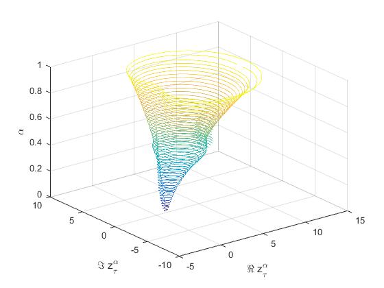
(a) hologram of $z^{\alpha}_{\tau}$ for all $\alpha$

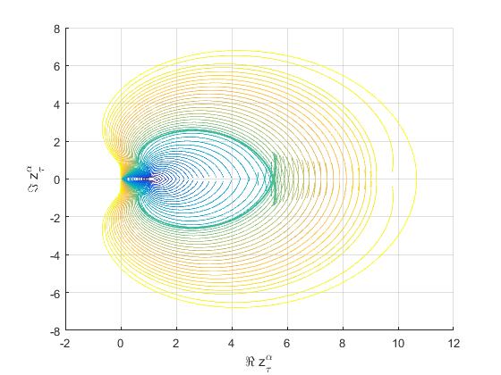
(b) top view of $z^{\alpha}_{\tau}$ for all $\alpha$

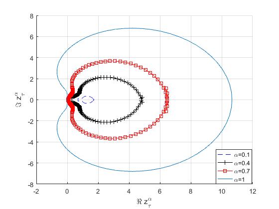
(c) plane graph of $z^{\alpha}_{\tau}$ for some $\alpha$

Figure 1: $z^{\alpha}_{\tau}\in\Sigma_{\theta_{0}}$ for $k=4$.

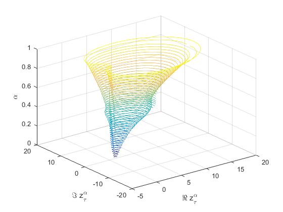
(a) hologram of $z^{\alpha}_{\tau}$ for all $\alpha$

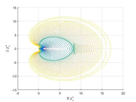
(b) top view of $z^{\alpha}_{\tau}$ for all $\alpha$

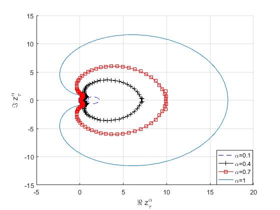
(c) plane graph of $z^{\alpha}_{\tau}$ for some $\alpha$

Figure 2: $z^{\alpha}_{\tau}\in\Sigma_{\theta_{0}}$ for $k=5$.

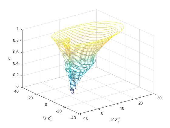
(a) hologram of $z^{\alpha}_{\tau}$ for all $\alpha$

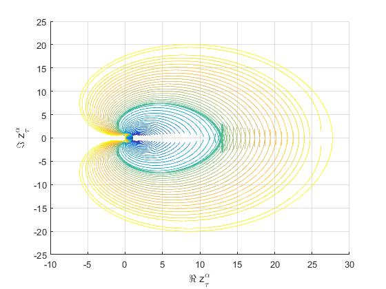
(b) top view of $z^{\alpha}_{\tau}$ for all $\alpha$

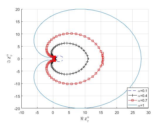
(c) plane graph of $z^{\alpha}_{\tau}$ for some $\alpha$

Figure 3: $z^{\alpha}_{\tau}\in\Sigma_{\theta_{0}}$ for $k=6$.

3.2 Error analysis for subdiffusion

We now give the error analysis of correction $L_{k}$ approximation (2.6) for (2.1). From (2.7), we know that

$$R_{k}(t_{n})=\frac{t_{n}^{k}}{k!}\partial^{k}_{t}f(0)+\left(\frac{t^{k}}{k!}\ast\partial^{k+1}_{t}f(t)\right)(t_{n}).$$

Then we introduce the following results.

Lemma 3.10

Let $V(t_{n})$ and $V^{n}$ be the solutions of (2.1) and (2.6), respectively. If $v=0$ and $f(t):=\frac{t^{k}}{k!}\partial^{k}_{t}f(0)$, then

$$\left\|V(t_{n})-V^{n}\right\|_{L^{2}(\Omega)}\leq c\tau^{k+1}t_{n}^{\alpha-1}\left\|\partial^{k}_{t}f(0)\right\|.$$

Proof

Using (2.9) and (2.16), there exist

$$V(t_{n})=\frac{1}{2\pi i}\int_{\Gamma_{\theta,\kappa}}{e^{zt_{n}}(z^{\alpha}-A)^{-1}\frac{1}{z^{k+1}}\partial^{k}_{t}f(0)}dz,$$

and

$$V^{n}=\frac{1}{2\pi i}\int_{\Gamma^{\tau}_{\theta,\kappa}}e^{zt_{n}}\left(z_{\tau}^{\alpha}-A\right)^{-1}\frac{\gamma_{k}(e^{-z\tau})}{k!}\tau^{k+1}\partial^{k}_{t}f(0)dz,$$

where $\theta\in(\pi/2,\pi)$ is sufficiently close to $\pi/2$ and $\kappa=t_{n}^{-1}$ in (2.10). It leads to

$$\begin{split}&V(t_{n})-V^{n}=J_{1}+J_{2}\end{split}$$

with

$$\begin{split}J_{1}=\frac{1}{2\pi i}\int_{\Gamma^{\tau}_{\theta,\kappa}}e^{zt_{n}}\left(\left(z^{\alpha}-A\right)^{-1}\frac{1}{z^{k+1}}-\left(z_{\tau}^{\alpha}-A\right)^{-1}\frac{\gamma_{k}(e^{-z\tau})}{k!}\tau^{k+1}\right)\partial^{k}_{t}f(0)dz,\end{split}$$

and

$$\begin{split}J_{2}=\frac{1}{2\pi i}\int_{\Gamma_{\theta,\kappa}\setminus\Gamma^{\tau}_{\theta,\kappa}}{e^{zt_{n}}\left(z^{\alpha}-A\right)^{-1}\frac{1}{z^{k+1}}\partial^{k}_{t}f(0)}dz.\end{split}$$

According to the triangle inequality, (2.12) and Lemmas 3.4,3.6,3.8,3.9, one has

$$\begin{split}\|J_{1}\|&\leq c\tau^{k+1-\alpha}\|\partial^{k}_{t}f(0)\|\left(\int^{\frac{\pi}{\tau\sin\theta}}_{\kappa}e^{rt_{n}\cos\theta}r^{-2\alpha}dr+\int^{\theta}_{-\theta}e^{\kappa t_{n}\cos\psi}\kappa^{1-2\alpha}d\psi\right)\\ &\leq c\tau^{k+1-\alpha}t_{n}^{2\alpha-1}\|\partial^{k}_{t}f(0)\|,\end{split}$$

for the last inequality, we use

$$\begin{split}&\int^{\frac{\pi}{\tau\sin\theta}}_{\kappa}e^{rt_{n}\cos\theta}r^{-2\alpha}dr=t_{n}^{2\alpha-1}\int^{\frac{t_{n}\pi}{\tau\sin\theta}}_{t_{n}\kappa}e^{s\cos\theta}s^{-2\alpha}ds\leq ct_{n}^{2\alpha-1},\\ &\int^{\theta}_{-\theta}e^{\kappa t_{n}\cos\psi}\kappa^{1-2\alpha}d\psi=t_{n}^{2\alpha-1}\int^{\theta}_{-\theta}e^{\kappa t_{n}\cos\psi}\left(\kappa t_{n}\right)^{1-2\alpha}d\psi\leq ct_{n}^{2\alpha-1}.\end{split}$$ (3.5)

From (2.12), it yields

$$\begin{split}\|J_{2}\|_{L^{2}(\Omega)}&\leq c\|\partial^{k}_{t}f(0)\|_{L^{2}(\Omega)}\int^{\infty}_{\frac{\pi}{\tau\sin\theta}}e^{rt_{n}\cos\theta}r^{-k-1-\alpha}dr\\ &\leq c\tau^{k+1-\alpha}\|\partial^{k}_{t}f(0)\|_{L^{2}(\Omega)}\int^{\infty}_{\frac{\pi}{\tau\sin\theta}}e^{rt_{n}\cos\theta}r^{-2\alpha}dr\leq c\tau^{k+1-\alpha}t_{n}^{2\alpha-1}\|\partial^{k}_{t}f(0)\|_{L^{2}(\Omega)}.\end{split}$$

Then the desired result is obtained.

Lemma 3.11

Let $V(t_{n})$ and $V^{n}$ be the solutions of (2.1) and (2.6), respectively. If $v=0$ and $f(t):=\frac{t^{k}}{k!}\ast\partial^{k+1}_{t}f(t)$, then

$$\left\|V(t_{n})-V^{n}\right\|\leq c\tau^{k+1-\alpha}\int_{0}^{t_{n}}(t_{n}-s)^{2\alpha-1}\left\|\partial^{k+1}_{s}f(s)\right\|ds.$$

Proof

By (2.9), we obtain

$$\begin{split}V(t_{n})&=\frac{1}{2\pi i}\int_{\Gamma_{\theta,\kappa}}{e^{zt_{n}}(z^{\alpha}-A)^{-1}\widehat{f}(z)}dz=(\mathscr{E}(t)\ast f(t))(t_{n})\\ &=\left(\mathscr{E}(t)\ast\left(\frac{t^{k}}{k!}\ast\partial^{k+1}_{t}f(t)\right)\right)(t_{n})=\left(\left(\mathscr{E}(t)\ast\frac{t^{k}}{k!}\right)\ast\partial^{k+1}_{t}f(t)\right)(t_{n})\end{split}$$ (3.6)

with

$$\mathscr{E}(t)=\frac{1}{2\pi i}\int_{\Gamma_{\theta,\kappa}}{e^{zt}(z^{\alpha}-A)^{-1}}dz.$$ (3.7)

From (2.15), it yields

$$\begin{split}\widetilde{V}(\xi)&=\left(z^{\alpha}_{\tau}-A\right)^{-1}\widetilde{f}(\xi)=\widetilde{\mathscr{E_{\tau}}}(\xi)\widetilde{f}(\xi)=\sum^{\infty}_{n=0}\mathscr{E}^{n}_{\tau}\xi^{n}\sum^{\infty}_{j=0}f^{j}\xi^{j}\\ &=\sum^{\infty}_{n=0}\sum^{\infty}_{j=0}\mathscr{E}^{n}_{\tau}f^{j}\xi^{n+j}=\sum^{\infty}_{j=0}\sum^{\infty}_{n=j}\mathscr{E}^{n-j}_{\tau}f^{j}\xi^{n}=\sum^{\infty}_{n=0}\sum^{n}_{j=0}\mathscr{E}^{n-j}_{\tau}f^{j}\xi^{n}=\sum^{\infty}_{n=0}V^{n}\xi^{n}\end{split}$$

with

$$V^{n}=\sum^{n}_{j=0}\mathscr{E}^{n-j}_{\tau}f^{j}:=\sum^{n}_{j=0}\mathscr{E}^{n-j}_{\tau}f(t_{j}).$$

Here $\sum^{\infty}_{n=0}\mathscr{E}^{n}_{\tau}\xi^{n}=\widetilde{\mathscr{E_{\tau}}}(\xi)=\left(z^{\alpha}_{\tau}-A\right)^{-1}$ and by Cauchy’s integral formula and the change of variables $\xi=e^{-z\tau}$ give the following representation for arbitrary $\rho\in(0,1)$

$$\mathscr{E}^{n}_{\tau}=\frac{1}{2\pi i}\int_{|\xi|=\rho}{\xi^{-n-1}\widetilde{\mathscr{E_{\tau}}}(\xi)}d\xi=\frac{\tau}{2\pi i}\int_{\Gamma^{\tau}_{\theta,\kappa}}{e^{zn\tau}\left(z^{\alpha}_{\tau}-A\right)^{-1}}dz,$$

where $\theta\in(\pi/2,\pi)$ is sufficiently close to $\pi/2$ and $\kappa=t_{n}^{-1}$ in (2.10).

According to Lemma 3.9 and (2.12), (3.5), there exists

$$\|\mathscr{E}^{n}_{\tau}\|\leq c\tau\left(\int^{\frac{\pi}{\tau\sin\theta}}_{\kappa}e^{rt_{n}\cos\theta}r^{-\alpha}dr+\int^{\theta}_{-\theta}e^{\kappa t_{n}\cos\psi}\kappa^{1-\alpha}d\psi\right)\leq c\tau t_{n}^{\alpha-1}.$$ (3.8)

Let $\mathscr{E}_{\tau}(t)=\sum^{\infty}_{n=0}\mathscr{E}^{n}_{\tau}\delta_{t_{n}}(t)$, with $\delta_{t_{n}}$ being the Dirac delta function at $t_{n}$. Then

$$\begin{split}(\mathscr{E}_{\tau}(t)\ast f(t))(t_{n})&=\left(\sum^{\infty}_{j=0}\mathscr{E}^{j}_{\tau}\delta_{t_{j}}(t)\ast f(t)\right)(t_{n})\\ &=\sum^{n}_{j=0}\mathscr{E}^{j}_{\tau}f(t_{n}-t_{j})=\sum^{n}_{j=0}\mathscr{E}^{n-j}_{\tau}f(t_{j})=V^{n}.\end{split}$$ (3.9)

Moreover, using the above equation and (2.13), there exist

$$\begin{split}\widetilde{(\mathscr{E}_{\tau}\ast t^{k})}(\xi)&=\sum^{\infty}_{n=0}\sum^{n}_{j=0}\mathscr{E}^{n-j}_{\tau}t_{j}^{k}\xi^{n}=\sum^{\infty}_{j=0}\sum^{\infty}_{n=j}\mathscr{E}^{n-j}_{\tau}t_{j}^{k}\xi^{n}=\sum^{\infty}_{j=0}\sum^{\infty}_{n=0}\mathscr{E}^{n}_{\tau}t_{j}^{k}\xi^{n+j}\\ &=\sum^{\infty}_{n=0}\mathscr{E}^{n}_{\tau}\xi^{n}\sum^{\infty}_{j=0}t_{j}^{k}\xi^{j}=\widetilde{\mathscr{E_{\tau}}}(\xi)\tau^{k}\sum^{\infty}_{j=0}j^{k}\xi^{j}=\widetilde{\mathscr{E}_{\tau}}(\xi)\tau^{k}\gamma_{k}(\xi).\end{split}$$

Using (3.6), (3.9) and Lemma 3.10, we have the following estimate

$$\left\|\left((\mathscr{E}_{\tau}-\mathscr{E})\ast\frac{t^{k}}{k!}\right)(t_{n})\right\|\leq c\tau^{k+1}t_{n}^{\alpha-1}.$$ (3.10)

Next, we prove the following inequality (3.11) for $t>0$

$$\left\|\left((\mathscr{E}_{\tau}-\mathscr{E})\ast\frac{t^{k}}{k!}\right)(t)\right\|\leq c\tau^{k+1}t^{\alpha-1},\quad\forall t\in(t_{n-1},t_{n}).$$ (3.11)

By Taylor series expansion of $\mathscr{E}(t)$ at $t=t_{n}$, we get

$$\begin{split}\left(\mathscr{E}\ast\frac{t^{k}}{k!}\right)(t)=&\left(\mathscr{E}\ast\frac{t^{k}}{k!}\right)(t_{n})+(t-t_{n})\left(\mathscr{E}\ast\frac{t^{k-1}}{(k-1)!}\right)(t_{n})+\cdots+\frac{(t-t_{n})^{k-1}}{(k-1)!}\left(\mathscr{E}\ast t\right)(t_{n})\\ &+\frac{(t-t_{n})^{k}}{k!}\left(\mathscr{E}\ast 1\right)(t_{n})+\frac{1}{k!}\int^{t}_{t_{n}}(t-s)^{k}\mathscr{E}(s)ds,\end{split}$$

which also holds for $\left(\mathscr{E}_{\tau}\ast\frac{t^{k}}{k!}\right)(t)$. Therefore, using (3.10), it yields

$$\left\|\left((\mathscr{E}_{\tau}-\mathscr{E})\ast\frac{t^{l}}{l!}\right)(t_{n})\right\|\leq c\tau^{l+1}t_{n}^{\alpha-1}.$$

According to (3.7), (2.12) and (3.5), one has

$$\begin{split}\|\mathscr{E}(t)\|\leq c\left(\int^{\infty}_{\kappa}e^{rt\cos\theta}r^{-\alpha}dr+\int^{\theta}_{-\theta}e^{\kappa t\cos\psi}\kappa^{1-\alpha}d\psi\right)\leq ct^{\alpha-1}.\end{split}$$

Moreover, we get

$$\left\|\int^{t}_{t_{n}}(t-s)^{k}\mathscr{E}(s)ds\right\|\leq c\int^{t_{n}}_{t}(s-t)^{k}s^{\alpha-1}ds\leq c\tau^{k+1}t^{\alpha-1}.$$

According to the definition of $\mathscr{E}_{\tau}(t)=\sum^{\infty}_{n=0}\mathscr{E}^{n}_{\tau}\delta_{t_{n}}(t)$ in (3.9) and (3.8), we deduce

$$\left\|\int^{t}_{t_{n}}(t-s)^{k}\mathscr{E}_{\tau}(s)ds\right\|\leq(t_{n}-t)^{k}\|\mathscr{E}^{n}_{\tau}\|\leq c\tau^{k+1}t_{n}^{\alpha-1}\leq c\tau^{k+1}t^{\alpha-1}~{}~{}~{}\forall t\in(t_{n-1},t_{n}).$$

By (3.10) and the above inequalities, it yields the inequality (3.11). The proof is completed.

Theorem 3.1

Let $V(t_{n})$ and $V^{n}$ be the solutions of (2.1) and (2.6), respectively. Let $v\in L^{2}(\Omega)$, $f\in C^{k}([0,T];L^{2}(\Omega))$ and $\int_{0}^{t}(t-s)^{2\alpha-1}\|\partial^{k+1}_{s}f(s)\|ds<\infty$ with $1\leq k\leq 6$. Then

$$\begin{split}&\left\|V^{n}-V(t_{n})\right\|\\ &\quad\leq C\tau^{k+1-\alpha}\left(t^{\alpha-(k+1)}_{n}\|v\|+\sum_{l=0}^{k}t^{2\alpha+l-(k+1)}_{n}\left\|\partial^{l}_{t}f(0)\right\|+\int_{0}^{t_{n}}(t_{n}-s)^{2\alpha-1}\|\partial^{k+1}_{s}f(s)\|ds\right).\end{split}$$

Proof

Subtracting (2.9) from (2.16), we obtain

$$V^{n}-V(t_{n})=I_{1}+\sum_{l=1}^{k-1}I_{2,l}+I_{3}-I_{4},$$

where

$$\begin{split}I_{1}=&\frac{1}{2\pi i}\int_{\Gamma^{\tau}}e^{zt_{n}}\left[\bar{\mu}(e^{-z\tau})K(z_{\tau})-K(z)\right](Av+f(0))dz,\\ I_{2,l}=&\frac{1}{2\pi i}\int_{\Gamma^{\tau}}e^{zt_{n}}\left[z_{\tau}\left(\frac{\gamma_{l}}{l!}+\sum_{j=1}^{k}d^{(k)}_{l,j}\xi^{j}\right)\tau^{l+1}K(z_{\tau})-z^{-l}K(z)\right]\partial^{l}_{t}f(0)dz,\\ \end{split}$$

and

$$\begin{split}I_{3}=&\frac{1}{2\pi i}\int_{\Gamma^{\tau}}e^{zt_{n}}z_{\tau}K(z_{\tau})\tau\widetilde{R_{k}}(e^{-z\tau})dz-\frac{1}{2\pi i}\int_{\Gamma}e^{zt_{n}}zK(z)\widehat{R_{k}}(z)dz,\\ I_{4}=&\frac{1}{2\pi i}\int_{\Gamma\backslash\Gamma^{\tau}}e^{zt_{n}}K(z)\left[Av+f(0)+\sum_{l=1}^{k-1}z^{-l}\partial^{l}_{t}f(0)\right]dz.\end{split}$$

Using the triangle inequality, Lemma 3.5, 3.6 and $\kappa=t_{n}^{-1}$, we estimate the first term

$$\begin{split}\left\|I_{1}\right\|\leq&C\int_{\Gamma^{\tau}}\left|e^{zt_{n}}\right|\left(\left\|\bar{\mu}(e^{-z\tau})K(z_{\tau})A-K(z)A\right\|\|v\|+\left\|\bar{\mu}(e^{-z\tau})K(z_{\tau})-K(z)\right\|\|f(0)\|\right)|dz|\\ \leq&C\tau^{k+1-\alpha}\int_{\Gamma^{\tau}}\left|e^{zt_{n}}\right|\left(|z|^{k-\alpha}\|v\|+|z|^{k-2\alpha}\|f(0)\|\right)|dz|\\ =&C\tau^{k+_{1}-\alpha}\left(t_{n}^{\alpha-(k+1)}\int^{\frac{t_{n}\pi}{\tau\sin\theta}}_{1}e^{rt_{n}\cos\theta}(rt_{n})^{k-\alpha}d(rt_{n})\|v\|+t_{n}^{\alpha-(k+1)}\int^{\theta}_{-\theta}e^{\cos\varphi}d\varphi\|v\|\right.\\ &\left.+t_{n}^{2\alpha-(k+1)}\int^{\frac{t_{n}\pi}{\tau\sin\theta}}_{1}e^{rt_{n}\cos\theta}(rt_{n})^{k-2\alpha}d(rt_{n})\|f(0)\|+t_{n}^{2\alpha-(k+1)}\int^{\theta}_{-\theta}e^{\cos\varphi}d\varphi\|f(0)\|\right)\\ \leq&C\tau^{k+1-\alpha}\left(t_{n}^{\alpha-(k+1)}\|v\|+t_{n}^{2\alpha-(k+1)}\|f(0)\|\right)\end{split}$$

Noting $(z^{\alpha}_{\tau}+A)^{-1}-(z^{\alpha}+A)^{-1}=(z^{\alpha}_{\tau}+A)^{-1}(z^{\alpha}+A)^{-1}(z^{\alpha}-z^{\alpha}_{\tau}),$ and according to the triangle inequality, (2.12) and Lemmas 3.7-3.9, we estimate the second term

$$\begin{split}\|I_{2,l}\|\leq&\frac{1}{2\pi}\int_{\Gamma^{\tau}}\left|e^{zt_{n}}\right|\left|\left(\frac{\gamma_{l}}{l!}+\sum_{j=1}^{k}d^{(k)}_{l,j}\xi^{j}\right)\tau^{l+1}-\frac{1}{z^{l+1}}\right|\left\|(z^{\alpha}_{\tau}+A)^{-1}\right\|\left\|\partial^{l}_{t}f(0)\right\||dz|\\ &+\frac{1}{2\pi}\int_{\Gamma^{\tau}}\left|e^{zt_{n}}\right||z|^{-l-1}\left\|(z^{\alpha}_{\tau}+A)^{-1}-(z^{\alpha}+A)^{-1}\right\|\left\|\partial^{l}_{t}f(0)\right\||dz|\\ \leq&C\int_{\Gamma^{\tau}}\left|e^{zt_{n}}\right|\tau^{k+1}|z|^{k-l-\alpha}\left\|\partial^{l}_{t}f(0)\right\||dz|+C\int_{\Gamma^{\tau}}\left|e^{zt_{n}}\right|\tau^{k+1-\alpha}|z|^{k-l-2\alpha}\left\|\partial^{l}_{t}f(0)\right\||dz|\\ \leq&C\tau^{k+1-\alpha}\int_{\Gamma^{\tau}}\left|e^{zt_{n}}\right||z|^{k-l-2\alpha}|dz|\left\|\partial^{l}_{t}f(0)\right\|\leq C\tau^{k+1-\alpha}t_{n}^{2\alpha+l-(k+1)}\left\|\partial^{l}_{t}f(0)\right\|.\end{split}$$

We next estimate $I_{4}$ as following. From the triangle inequality and the resolvent estimate (2.12), it yields

$$\begin{split}\left\|I_{4}\right\|\leq&C\int_{\Gamma\backslash\Gamma^{\tau}}\left|e^{zt_{n}}\right|\left\|K(z)A\right\|\left\|v\right\|dz+C\int_{\Gamma\backslash\Gamma^{\tau}}\left|e^{zt_{n}}\right|\left\|K(z)\right\|\left\|f(0)\right\||dz|\\ &+C\int_{\Gamma\backslash\Gamma^{\tau}}\left|e^{zt_{n}}\right|\left\|K(z)\right\|\sum_{l=1}^{k-1}|z|^{-l}\left\|\partial^{l}_{t}f(0)\right\||dz|\\ \leq&C\int_{\Gamma\backslash\Gamma^{\tau}}\left|e^{zt_{n}}\right||z|^{-1}\left\|v\right\|dz+C\int_{\Gamma\backslash\Gamma^{\tau}}\left|e^{zt_{n}}\right||z|^{-1-\alpha}\left\|f(0)\right\||dz|\\ &+C\int_{\Gamma\backslash\Gamma^{\tau}}\left|e^{zt_{n}}\right|\sum_{l=1}^{k-1}|z|^{-l-1-\alpha}\left\|\partial^{l}_{t}f(0)\right\||dz|\\ \leq&C\tau^{k+1-\alpha}\left(t_{n}^{\alpha-(k+1)}\left\|v\right\|+t_{n}^{2\alpha-(k+1)}\left\|f(0)\right\||dz|+\sum_{l=1}^{k-1}t_{n}^{2\alpha+l-(k+1)}\left\|\partial^{l}_{t}f(0)\right\|\right).\end{split}$$

Since

$$\begin{split}\int_{\Gamma\backslash\Gamma^{\tau}}\left|e^{zt_{n}}\right||z|^{-1}|dz|\left\|v\right\|=&\int^{\infty}_{\frac{\pi}{\tau\sin\theta}}\left|e^{zt_{n}}\right||z|^{-1}|dz|\left\|v\right\|\leq\int^{\infty}_{\frac{\pi}{\tau\sin\theta}}e^{rt_{n}\cos\theta}r^{-1}dr\left\|v\right\|\\ \leq&\tau^{k+1-\alpha}\int^{\infty}_{\frac{\pi}{\tau\sin\theta}}e^{rt_{n}\cos\theta}r^{k-\alpha}dr\left\|v\right\|\leq\tau^{k+1-\alpha}t_{n}^{\alpha-(k+1)}\left\|v\right\|\end{split}$$

with $1\leq\left(\frac{\sin\theta}{\pi}\right)^{k+1-\alpha}\tau^{k+1-\alpha}r^{k+1-\alpha}\leq\tau^{k+1-\alpha}r^{k+1-\alpha}$, $r\geq\frac{\pi}{\tau\sin\theta}$.

According to Lemmas 3.10 and 3.11 with $R_{k}=\frac{t^{k}}{k!}\partial^{k}_{t}f(0)+\frac{t^{k}}{k!}\ast\partial^{k+1}_{t}f(t)$, there exist

$$\left\|I_{3}\right\|\leq c\tau^{k+1}t_{n}^{\alpha-1}\left\|\partial^{k}_{t}f(0)\right\|+c\tau^{k+1}\int_{0}^{t_{n}}(t_{n}-s)^{2\alpha-1}\left\|\partial^{k+1}_{s}f(s)\right\|ds.$$

The proof is completed.

4 Numerical results

We numerically verify the above theoretical results and the discrete $L^{2}$-norm is used to measure the numerical errors. In the space direction, it is discretized with the spectral collocation method with the Chebyshev-Gauss-Lobatto points ACYZ:21 ; STW:2011 . Here we main focus on the time direction convergence order, since the convergence rate of the spatial discretization is well understood.

Example 1

Let us consider the following subdiffusion (1.1)

$$\begin{split}&{}^{C}_{0}D^{\alpha}_{t}u(x,t)-\frac{\partial^{2}u(x,t)}{\partial x^{2}}=f(x,t),\\ &u(-1,t)=u(1,t)=0,\\ &u(x,0)=v(x)\end{split}$$

with the nonsmooth data $v(x)=\sqrt{1-x^{2}}$ and $f(x,t)=(t+1)^{8}\left(1+\chi_{(0,1)}(x)\right)$. Here

$$\chi_{(0,1)}(x)=\left\{\begin{array}[]{l@{\quad} l}1,~{}~{}~{}~{}0<x<1,\\ 0,~{}~{}~{}~{}{\rm elsewhere}.\end{array}\right.$$

Since the analytic solutions is unknown, the order of the convergence of the numerical results are computed by the following formula

$${\rm Convergence~{}Rate}=\frac{\ln\left(||u^{N/2}-u^{N}||/||u^{N}-u^{2N}||\right)}{\ln 2}$$

with $u^{N}=V^{N}+v$ in (2.6).

Table 5: The errors and convergent order of uncorrection $L_{k}$ approximation (2.5).

$k$	$\alpha$	$N=80$	$N=160$	$N=320$	$N=640$	$N=1280$	Rate
4	0.2	4.8406e-04	2.3850e-04	1.1712e-04	5.7975e-05	2.8839e-05	$\approx$ 1.0173
	0.5	1.0889e-03	5.6592e-04	2.7928e-04	1.3829e-04	6.8792e-05	$\approx$ 0.9961
	0.8	1.4043e-03	8.8681e-04	4.4652e-04	2.2157e-04	1.1023e-04	$\approx$ 0.9178
5	0.2	4.9653e-04	2.3900e-04	1.1713e-04	5.7975e-05	2.8840e-05	$\approx$ 1.0265
	0.5	1.1835e-03	5.7040e-04	2.7948e-04	1.3830e-04	6.8792e-05	$\approx$ 1.0261
	0.8	1.8875e-03	9.1481e-04	4.4809e-04	2.2166e-04	1.1023e-04	$\approx$ 1.0245
6	0.2	4.9694e-04	2.3901e-04	1.1714e-04	5.7975e-05	2.8840e-05	$\approx$ 1.0268
	0.5	1.2767e-03	5.7052e-04	2.7949e-04	1.3830e-04	6.8792e-05	$\approx$ 1.0535
	0.8	1.6587e-03	9.1580e-04	4.4811e-04	2.2166e-04	1.1023e-04	$\approx$ 0.9778

Table 6: The errors and convergent order of correction $L_{k}$ approximation (2.6).

$k$	$\alpha$	$N=20$	$N=40$	$N=80$	$N=160$	$N=320$	Rate
4	0.2	7.9510e-03	3.1598e-04	1.2879e-05	5.0269e-07	1.9150e-08	$\approx$ 4.6658(4.8)
	0.5	3.4422e-02	2.0224e-03	9.7963e-05	4.5534e-06	2.0704e-07	$\approx$ 4.3358(4.5)
	0.8	1.3454e-01	8.5003e-03	5.0322e-04	2.8569e-05	1.5882e-06	$\approx$ 4.0926(4.2)
5	0.2	6.0454e-03	9.2733e-06	4.1798e-07	8.0735e-09	1.5835e-10	$\approx$ 6.2965(5.8)
	0.5	1.2783e-02	1.8653e-04	3.2579e-06	7.9314e-08	1.8079e-09	$\approx$ 5.6884(5.5)
	0.8	1.9116e-02	2.8855e-04	2.0050e-05	5.5691e-07	1.5410e-08	$\approx$ 5.0606(5.2)
6	0.2	1.3275e-01	1.1518e-03	2.4273e-08	7.6887e-11	1.4921e-11	$\approx$ 8.2626(6.8)
	0.5	3.4652e-01	2.7804e-02	4.2374e-04	2.9762e-07	1.2242e-10	$\approx$ 7.8494(6.5)
	0.8	2.5905e-01	2.8118e-02	1.4048e-03	2.8657e-06	2.6575e-10	$\approx$ 7.4650(6.2)

Table 5 shows that the stand $L_{k}$ approximation in (2.5) just achieves the first-order convergence. However, the correction $L_{k}$ in (2.6) preserves the high-order convergence rate with nonsmooth data in Table 6.

Appendix

The coefficients $\omega^{(k)}_{j}$ of $L_{k}$ approximation in (2.4) are given explicitly by the following

• $L_{1}$ approximation

  $$\begin{split}\omega^{(1)}_{0}=\frac{1}{\Gamma(2-\alpha)},\quad\omega^{(1)}_{j}=\frac{(j+1)^{1-\alpha}-2j^{1-\alpha}+(j-1)^{1-\alpha}}{\Gamma(2-\alpha)},~{}~{}j\geq 1.\end{split}$$

• $L_{2}$ approximation

  $$\begin{split}\omega^{(2)}_{0}=\frac{1}{\Gamma(3-\alpha)}+\frac{1}{2}\frac{1}{\Gamma(2-\alpha)},\quad\omega^{(2)}_{1}=\frac{\left(2^{2-\alpha}-3\right)}{\Gamma(3-\alpha)}+\frac{1}{2}\frac{\left(2^{1-\alpha}-3\right)}{\Gamma(2-\alpha)},\end{split}$$

  $$\begin{split}\omega^{(2)}_{j}=&\frac{\left((j+1)^{2-\alpha}-3j^{2-\alpha}+3(j-1)^{2-\alpha}-(j-2)^{2-\alpha}\right)}{\Gamma(3-\alpha)}+\frac{1}{2}\frac{\left((j+1)^{1-\alpha}-3j^{1-\alpha}+3(j-1)^{1-\alpha}-(j-2)^{1-\alpha}\right)}{\Gamma(2-\alpha)},~{}~{}j\geq 2.\end{split}$$

• $L_{3}$ approximation

  $$\begin{split}\omega^{(3)}_{0}=\frac{1}{\Gamma(4-\alpha)}+\frac{1}{\Gamma(3-\alpha)}+\frac{1}{3}\frac{1}{\Gamma(2-\alpha)},\quad\omega^{(3)}_{1}=\frac{2^{3-\alpha}-4}{\Gamma(4-\alpha)}+\frac{2^{2-\alpha}-4}{\Gamma(3-\alpha)}+\frac{1}{3}\frac{2^{1-\alpha}-4}{\Gamma(2-\alpha)},\end{split}$$

  $$\begin{split}\omega^{(3)}_{2}=&\frac{3^{3-\alpha}-4\times 2^{3-\alpha}+6}{\Gamma(4-\alpha)}+\frac{3^{2-\alpha}-4\times 2^{2-\alpha}+6}{\Gamma(3-\alpha)}+\frac{1}{3}\frac{3^{1-\alpha}-4\times 2^{1-\alpha}+6}{\Gamma(2-\alpha)},\end{split}$$

  $$\begin{split}\omega^{(3)}_{j}=&\frac{(j+1)^{3-\alpha}-4j^{4-\alpha}+6(j-1)^{3-\alpha}-4(j-2)^{3-\alpha}+(j-3)^{3-\alpha}}{\Gamma(4-\alpha)}+\frac{(j+1)^{2-\alpha}-4j^{2-\alpha}+6(j-1)^{2-\alpha}-4(j-2)^{2-\alpha}+(j-3)^{2-\alpha}}{\Gamma(3-\alpha)}\\ &+\frac{1}{3}\frac{(j+1)^{1-\alpha}-4j^{1-\alpha}+6(j-1)^{1-\alpha}-4(j-2)^{1-\alpha}+(j-3)^{1-\alpha}}{\Gamma(2-\alpha)},~{}j\geq 3.\end{split}$$

• $L_{4}$ approximation

  $$\begin{split}\omega^{(4)}_{0}=\frac{1}{\Gamma(5-\alpha)}+\frac{3}{2}\frac{1}{\Gamma(4-\alpha)}+\frac{11}{12}\frac{1}{\Gamma(3-\alpha)}+\frac{1}{4}\frac{1}{\Gamma(2-\alpha)},\quad\omega^{(4)}_{1}=\frac{2^{4-\alpha}-5}{\Gamma(5-\alpha)}+\frac{3}{2}\frac{2^{3-\alpha}-5}{\Gamma(4-\alpha)}+\frac{11}{12}\frac{2^{2-\alpha}-5}{\Gamma(3-\alpha)}+\frac{1}{4}\frac{2^{1-\alpha}-5}{\Gamma(2-\alpha)},\end{split}$$

  $$\begin{split}\omega^{(4)}_{2}=\frac{3^{4-\alpha}-5\times 2^{4-\alpha}+10}{\Gamma(5-\alpha)}+\frac{3}{2}\frac{3^{3-\alpha}-5\times 2^{3-\alpha}+10}{\Gamma(4-\alpha)}+\frac{11}{12}\frac{3^{2-\alpha}-5\times 2^{2-\alpha}+10}{\Gamma(3-\alpha)}+\frac{1}{4}\frac{3^{1-\alpha}-5\times 2^{1-\alpha}+10}{\Gamma(2-\alpha)},\end{split}$$

  $$\begin{split}\omega^{(4)}_{3}=&\frac{4^{4-\alpha}-5\times 3^{4-\alpha}+10\times 2^{4-\alpha}-10}{\Gamma(5-\alpha)}+\frac{3}{2}\frac{4^{3-\alpha}-5\times 3^{3-\alpha}+10\times 2^{3-\alpha}-10}{\Gamma(4-\alpha)}\\ &+\frac{11}{12}\frac{4^{2-\alpha}-5\times 3^{2-\alpha}+10\times 2^{2-\alpha}-10}{\Gamma(3-\alpha)}+\frac{1}{4}\frac{4^{1-\alpha}-5\times 3^{1-\alpha}+10\times 2^{1-\alpha}-10}{\Gamma(2-\alpha)},\end{split}$$

  $$\begin{split}\omega^{(4)}_{j}=&\frac{(j+1)^{4-\alpha}-5j^{4-\alpha}+10(j-1)^{4-\alpha}-10(j-2)^{4-\alpha}+5(j-3)^{4-\alpha}-(j-4)^{4-\alpha}}{\Gamma(5-\alpha)}\\ &+\frac{3}{2}\frac{(j+1)^{3-\alpha}-5j^{3-\alpha}+10(j-1)^{3-\alpha}-10(j-2)^{3-\alpha}+5(j-3)^{3-\alpha}-(j-4)^{3-\alpha}}{\Gamma(4-\alpha)}\\ &+\frac{11}{12}\frac{(j+1)^{2-\alpha}-5j^{2-\alpha}+10(j-1)^{2-\alpha}-10(j-2)^{2-\alpha}+5(j-3)^{2-\alpha}-(j-4)^{2-\alpha}}{\Gamma(3-\alpha)}\\ &+\frac{1}{4}\frac{(j+1)^{1-\alpha}-5j^{1-\alpha}+10(j-1)^{1-\alpha}-10(j-2)^{1-\alpha}+5(j-3)^{1-\alpha}-(j-4)^{1-\alpha}}{\Gamma(2-\alpha)},~{}j\geq 4.\end{split}$$

• $L_{5}$ approximation

  $$\begin{split}\omega^{(5)}_{0}=&\frac{1}{\Gamma(6-\alpha)}+2\frac{1}{\Gamma(5-\alpha)}+\frac{7}{4}\frac{1}{\Gamma(4-\alpha)}+\frac{5}{6}\frac{1}{\Gamma(3-\alpha)}+\frac{1}{5}\frac{1}{\Gamma(2-\alpha)},\end{split}$$

  $$\begin{split}\omega^{(5)}_{1}=&\frac{2^{5-\alpha}-6}{\Gamma(6-\alpha)}+2\frac{2^{4-\alpha}-6}{\Gamma(5-\alpha)}+\frac{7}{4}\frac{2^{3-\alpha}-6}{\Gamma(4-\alpha)}+\frac{5}{6}\frac{2^{2-\alpha}-6}{\Gamma(3-\alpha)}+\frac{1}{5}\frac{2^{1-\alpha}-6}{\Gamma(2-\alpha)},\end{split}$$

  $$\begin{split}\omega^{(5)}_{2}=&\frac{3^{5-\alpha}-6\times 2^{5-\alpha}+15}{\Gamma(6-\alpha)}+2\frac{3^{4-\alpha}-6\times 2^{4-\alpha}+15}{\Gamma(5-\alpha)}+\frac{7}{4}\frac{3^{3-\alpha}-6\times 2^{3-\alpha}+15}{\Gamma(4-\alpha)}+\frac{5}{6}\frac{3^{2-\alpha}-6\times 2^{2-\alpha}+15}{\Gamma(3-\alpha)}+\frac{1}{5}\frac{3^{1-\alpha}-6\times 2^{1-\alpha}+15}{\Gamma(2-\alpha)},\end{split}$$

  $$\begin{split}\omega^{(5)}_{3}=&\frac{4^{5-\alpha}-6\times 3^{5-\alpha}+15\times 2^{5-\alpha}-20}{\Gamma(6-\alpha)}+2\frac{4^{4-\alpha}-6\times 3^{4-\alpha}+15\times 2^{4-\alpha}-20}{\Gamma(5-\alpha)}+\frac{7}{4}\frac{4^{3-\alpha}-6\times 3^{3-\alpha}+15\times 2^{3-\alpha}-20}{\Gamma(4-\alpha)}\\ &+\frac{5}{6}\frac{4^{2-\alpha}-6\times 3^{2-\alpha}+15\times 2^{2-\alpha}-20}{\Gamma(3-\alpha)}+\frac{1}{5}\frac{4^{1-\alpha}-6\times 3^{1-\alpha}+15\times 2^{1-\alpha}-20}{\Gamma(2-\alpha)},\end{split}$$

  $$\begin{split}\omega^{(5)}_{4}=&\frac{5^{5-\alpha}-6\times 4^{5-\alpha}+15\times 3^{5-\alpha}-20\times 2^{5-\alpha}+15}{\Gamma(6-\alpha)}+2\frac{5^{4-\alpha}-6\times 4^{4-\alpha}+15\times 3^{4-\alpha}-20\times 2^{4-\alpha}+15}{\Gamma(5-\alpha)}\\ &+\frac{7}{4}\frac{5^{3-\alpha}-6\times 4^{3-\alpha}+15\times 3^{3-\alpha}-20\times 2^{3-\alpha}+15}{\Gamma(4-\alpha)}+\frac{5}{6}\frac{5^{2-\alpha}-6\times 4^{2-\alpha}+15\times 3^{2-\alpha}-20\times 2^{2-\alpha}+15}{\Gamma(3-\alpha)}\\ &+\frac{1}{5}\frac{(5^{1-\alpha}-6\times 4^{1-\alpha}+15\times 3^{1-\alpha}-20\times 2^{1-\alpha}+15}{\Gamma(2-\alpha)},\end{split}$$

  $$\begin{split}\omega^{(5)}_{j}=&\frac{(j+1)^{5-\alpha}-6j^{5-\alpha}+15(j-1)^{5-\alpha}-20(j-2)^{5-\alpha}+15(j-3)^{5-\alpha}-6(j-4)^{5-\alpha}+(j-5)^{5-\alpha}}{\Gamma(6-\alpha)}\\ &+2\frac{(j+1)^{4-\alpha}-6j^{4-\alpha}+15(j-1)^{4-\alpha}-20(j-2)^{4-\alpha}+15(j-3)^{4-\alpha}-6(j-4)^{4-\alpha}+(j-5)^{4-\alpha}}{\Gamma(5-\alpha)}\\ &+\frac{7}{4}\frac{(j+1)^{3-\alpha}-6j^{3-\alpha}+15(j-1)^{3-\alpha}-20(j-2)^{3-\alpha}+15(j-3)^{3-\alpha}-6(j-4)^{3-\alpha}+(j-5)^{3-\alpha}}{\Gamma(4-\alpha)}\\ &+\frac{5}{6}\frac{(j+1)^{2-\alpha}-6j^{2-\alpha}+15(j-1)^{2-\alpha}-20(j-2)^{2-\alpha}+15(j-3)^{2-\alpha}-6(j-4)^{2-\alpha}+(j-5)^{2-\alpha}}{\Gamma(3-\alpha)}\\ &+\frac{1}{5}\frac{(j+1)^{1-\alpha}-6j^{1-\alpha}+15(j-1)^{1-\alpha}-20(j-2)^{1-\alpha}+15(j-3)^{1-\alpha}-6(j-4)^{1-\alpha}+(j-5)^{1-\alpha}}{\Gamma(2-\alpha)},~{}j\geq 5.\end{split}$$

• $L_{6}$ approximation

  $$\begin{split}\omega^{(6)}_{0}=&\frac{1}{\Gamma(7-\!\alpha)}\!+\!\frac{5}{2}\frac{1}{\Gamma(6-\!\alpha)}\!+\!\frac{17}{6}\frac{1}{\Gamma(5-\!\alpha)}\!+\!\frac{15}{8}\frac{1}{\Gamma(4-\!\alpha)}\!+\!\frac{137}{180}\frac{1}{\Gamma(3-\!\alpha)}\!+\!\frac{1}{6}\frac{1}{\Gamma(2-\!\alpha)},\end{split}$$

  $$\begin{split}\omega^{(6)}_{1}\!\!=\!&\frac{\ 2^{6-\alpha}-7}{\Gamma(7-\!\alpha)}\!+\!\frac{5}{2}\frac{2^{5-\alpha}-7}{\Gamma(6-\!\alpha)}\!+\!\frac{17}{6}\frac{2^{4-\alpha}-7}{\Gamma(5-\!\alpha)}\!+\!\frac{15}{8}\frac{2^{3-\alpha}-7}{\Gamma(4-\!\alpha)}\!+\!\frac{137}{180}\frac{2^{2-\alpha}-7}{\Gamma(3-\!\alpha)}\!+\!\frac{1}{6}\frac{2^{1-\alpha}-7}{\Gamma(2-\!\alpha)},\end{split}$$

  $$\begin{split}\omega^{(6)}_{2}=&\frac{3^{6-\alpha}-7\times 2^{6-\alpha}+21}{\Gamma(7-\alpha)}+\frac{5}{2}\frac{3^{5-\alpha}-7\times 2^{5-\alpha}+21}{\Gamma(6-\alpha)}+\frac{17}{6}\frac{3^{4-\alpha}-7\times 2^{4-\alpha}+21}{\Gamma(5-\alpha)}\\ &+\frac{15}{8}\frac{3^{3-\alpha}-7\times 2^{3-\alpha}+21}{\Gamma(4-\alpha)}+\frac{137}{180}\frac{3^{2-\alpha}-7\times 2^{2-\alpha}+21}{\Gamma(3-\alpha)}+\frac{1}{5}\frac{3^{1-\alpha}-7\times 2^{1-\alpha}+21}{\Gamma(2-\alpha)},\end{split}$$

  $$\begin{split}\omega^{(6)}_{3}=&\frac{4^{6-\alpha}-7\times 3^{6-\alpha}+21\times 2^{6-\alpha}-35}{\Gamma(7-\alpha)}+\frac{5}{2}\frac{4^{5-\alpha}-7\times 3^{5-\alpha}+21\times 2^{5-\alpha}-35}{\Gamma(6-\alpha)}+\frac{17}{6}\frac{4^{4-\alpha}-7\times 3^{4-\alpha}+21\times 2^{4-\alpha}-35}{\Gamma(5-\alpha)}\\ &+\frac{15}{8}\frac{4^{3-\alpha}-7\times 3^{3-\alpha}+21\times 2^{3-\alpha}-35}{\Gamma(4-\alpha)}+\frac{137}{180}\frac{4^{2-\alpha}-7\times 3^{2-\alpha}+21\times 2^{2-\alpha}-35}{\Gamma(3-\alpha)}+\frac{1}{6}\frac{4^{1-\alpha}-7\times 3^{1-\alpha}+21\times 2^{1-\alpha}-35}{\Gamma(2-\alpha)},\end{split}$$

  $$\begin{split}\omega^{(6)}_{4}=&\frac{5^{6-\alpha}-7\times 4^{6-\alpha}+21\times 3^{6-\alpha}-35\times 2^{6-\alpha}+35}{\Gamma(7-\alpha)}+\frac{5}{2}\frac{5^{5-\alpha}-7\times 4^{5-\alpha}+21\times 3^{5-\alpha}-35\times 2^{5-\alpha}+35}{\Gamma(6-\alpha)}\\ &+\frac{17}{6}\frac{5^{4-\alpha}-7\times 4^{4-\alpha}+21\times 3^{4-\alpha}-35\times 2^{4-\alpha}+35}{\Gamma(5-\alpha)}+\frac{15}{8}\frac{5^{3-\alpha}-7\times 4^{3-\alpha}+21\times 3^{3-\alpha}-35\times 2^{3-\alpha}+35}{\Gamma(4-\alpha)}\\ &+\frac{137}{180}\frac{5^{2-\alpha}-7\times 4^{2-\alpha}+21\times 3^{2-\alpha}-35\times 2^{2-\alpha}+35}{\Gamma(3-\alpha)}+\frac{1}{6}\frac{5^{1-\alpha}-7\times 4^{1-\alpha}+21\times 3^{1-\alpha}-35\times 2^{1-\alpha}+35}{\Gamma(2-\alpha)},\end{split}$$

  $$\begin{split}\omega^{(6)}_{5}=&\frac{6^{6-\alpha}-7\times 5^{6-\alpha}+21\times 4^{6-\alpha}-35\times 3^{6-\alpha}+35\times 2^{6-\alpha}-21}{\Gamma(7-\alpha)}+\frac{5}{2}\frac{6^{5-\alpha}-7\times 5^{5-\alpha}+21\times 4^{5-\alpha}-35\times 3^{5-\alpha}+35\times 2^{5-\alpha}-21}{\Gamma(6-\alpha)}\\ &+\frac{17}{6}\frac{6^{4-\alpha}-7\times 5^{4-\alpha}+21\times 4^{4-\alpha}-35\times 3^{4-\alpha}+35\times 2^{4-\alpha}-21}{\Gamma(5-\alpha)}+\frac{15}{8}\frac{6^{3-\alpha}-7\times 5^{3-\alpha}+21\times 4^{3-\alpha}-35\times 3^{3-\alpha}+35\times 2^{3-\alpha}-21}{\Gamma(4-\alpha)}\\ &+\frac{137}{180}\frac{6^{2-\alpha}-7\times 5^{2-\alpha}+21\times 4^{2-\alpha}-35\times 3^{2-\alpha}+35\times 2^{2-\alpha}-21}{\Gamma(3-\alpha)}+\frac{1}{6}\frac{6^{1-\alpha}-7\times 5^{1-\alpha}+21\times 4^{1-\alpha}-35\times 3^{1-\alpha}+35\times 2^{1-\alpha}-21}{\Gamma(2-\alpha)},\end{split}$$

  $$\begin{split}\omega^{(6)}_{j}=&\frac{(j+1)^{6-\alpha}-7j^{6-\alpha}+21(j-1)^{6-\alpha}-35(j-2)^{6-\alpha}+35(j-3)^{6-\alpha}-21(j-4)^{6-\alpha}+7(j-5)^{6-\alpha}-(j-6)^{6-\alpha}}{\Gamma(7-\alpha)}\\ &+\frac{5}{2}\frac{(j+1)^{5-\alpha}-7j^{5-\alpha}+21(j-1)^{5-\alpha}-35(j-2)^{5-\alpha}+35(j-3)^{5-\alpha}-21(j-4)^{5-\alpha}+7(j-5)^{5-\alpha}-(j-6)^{5-\alpha}}{\Gamma(6-\alpha)}\\ &+\frac{17}{6}\frac{(j+1)^{4-\alpha}-7j^{4-\alpha}+21(j-1)^{4-\alpha}-35(j-2)^{4-\alpha}+35(j-3)^{4-\alpha}-21(j-4)^{4-\alpha}+7(j-5)^{4-\alpha}-(j-6)^{4-\alpha}}{\Gamma(5-\alpha)}\\ &+\frac{15}{8}\frac{(j+1)^{3-\alpha}-7j^{3-\alpha}+21(j-1)^{3-\alpha}-35(j-2)^{3-\alpha}+35(j-3)^{3-\alpha}-21(j-4)^{3-\alpha}+7(j-5)^{3-\alpha}-(j-6)^{3-\alpha}}{\Gamma(4-\alpha)}\\ &+\frac{137}{180}\frac{(j+1)^{2-\alpha}-7j^{2-\alpha}+21(j-1)^{2-\alpha}-35(j-2)^{2-\alpha}+35(j-3)^{2-\alpha}-21(j-4)^{2-\alpha}+7(j-5)^{2-\alpha}-(j-6)^{2-\alpha}}{\Gamma(3-\alpha)}\\ &+\frac{1}{6}\frac{(j+1)^{1-\alpha}-7j^{1-\alpha}+21(j-1)^{1-\alpha}-35(j-2)^{1-\alpha}+35(j-3)^{1-\alpha}-21(j-4)^{1-\alpha}+7(j-5)^{1-\alpha}-(j-6)^{1-\alpha}}{\Gamma(2-\alpha)},~{}j\geq 6.\end{split}$$

Data availability

I confirm I have included a data availability statement in my main manuscript file.

Declarations

Funding: This work was supported by NSFC 11601206 and Hong Kong RGC grant (No. 25300818).

Conflicts of interest/Competing interests: The authors have no conflicts of interest to declare that are relevant to the content of this article.

Availability of data and material: Not applicable.

Code availability: Not applicable.

Authors’ contributions: An equal contribution.

References

- (1) Akrivis G., Chen M.H., Yu, F., Zhou, Z.: The energy technique for the six-step BDF method. SIAM J. Numer. Anal. 59, 2449-2472 (2021)
- (2) Appel K.I.: The use of the computer in the proof of the four color theorem. Proc. Amer. Philos. Soc. 128, 35-39 (1984)
- (3) Cao J.X., Li C.P., Chen Y.Q.: High-order approximation to Caputo derivatives and Caputo-type advection-diffusion equations (II). Fract. Calc. Appl. Anal. 18, 735-761 (2015)
- (4) Bhagat V., Bhattacharya R., Roy D.: On the evaluation of generalized Bose-Einstein and Fermi-Dirac integrals. Comput. Phys. Comm. 155, 7-20 (2003)
- (5) Chen M.H., Jiang S.Z., Bu W.P.: Two schemes on graded meshes for fractional Feynman-Kac equation. J. Sci. Comput. 88, 58 (2021)
- (6) Chen M.H., Deng W.H.: Discretized fractional substantial calculus. ESAIM: Math. Model. Numer. Anal. 49, 373-394 (2015)
- (7) Chen M.H., Deng W.H.: Fourth order accurate scheme for the space fractional diffusion equations. SIAM J. Numer. Anal. 52, 1418-1438 (2014)
- (8) Flajolet P.: Singularity analysis and asymptotics of Bernoulli sums. Theoret. Comput. Sci. 215, 371-381 (1999)
- (9) Gao G.H., Sun Z.Z., Zhang H.W.: A new fractional numerical differentiation formula to approximate the Caputo fractional derivative and its applications. J. Comput. Phys. 259, 33-50 (2014)
- (10) Jin B., Li B.Y., Zhou Z.: Correction of high-order BDF convolution quadrature for fractional evolution equations. SIAM J. Sci. Comput. 39, A3129-A3152 (2017)
- (11) Jin B., Lazarov R., Zhou Z.: An analysis of the scheme for the subdiffusion equation with nonsmooth data. IMA J. Numer. Anal. 36, 197-221 (2016)
- (12) Kopteva N.: Error analysis of an -type method on graded meshes for a fractional-order parabolic problem. Math. Comp. 90, 19-40 (2021)
- (13) LeVeque R.J.: Finite Difference Methods for Ordinary and Partial Differential Equations. SIAM, Philadelphia (2007)
- (14) Li H.F., Cao J.X., Li C.P.: High-order approximation to Caputo derivatives and Caputo-type advection-diffusion equations (III). J. Comput. Appl. Math. 299, 159-175 (2016)
- (15) Lin Y.M., Xu C.J.: Finite difference/spectral approximations for the time-fractional diffusion equation. J. Comput. Phys. 225, 1533-1552 (2007)
- (16) Lubich Ch.: Discretized fractional calculus. SIAM J. Math. Anal. 17, 704-719 (1986)
- (17) Lubich Ch., Sloan I.H., Thomée V.: Nonsmooth data error estimates for approximations of an evolution equation with a positive-type memory term. Math. Comp. 65, 1-17 (1996)
- (18) Lv C.W., Xu C.J.: Error analysis of a high order method for time-fractional diffusion equations. SIAM J. Sci. Comput. 38, A2699-A2724 (2016)
- (19) Meerschaert M.M., Tadjeran C.: Finite difference approximations for fractional advection-dispersion flow equations. J. Comput. Appl. Math. 172, 65-77 (2004)
- (20) Metzler R., Klafter J.: The random walk’s guide to anomalous diffusion: a fractional dynamics approach. Phys. Rep. 339, 1–77 (2000)
- (21) Podlubny I.: Fractional Differential Equations. Academic Press, New York (1999)
- (22) Sakamoto K., Yamamoto M.: Initial value/boundary value problems for fractional diffusion-wave equations and applications to some inverse problems. J. Math. Anal. Appl. 382, 426–447 (2011)
- (23) Shen J., Tang T., Wang L.: Spectral Methods: Algorithms, Analysis and Applications. Springer-Verlag, Berlin (2011)
- (24) Shi J.K., Chen M.H.: Correction of high-order BDF convolution quadrature for fractional Feynman-Kac equation with Lévy flight. J. Sci. Comput. 85, 28 (2020).
- (25) Stynes M., O’riordan E., Gracia J.L.: Error analysis of a finite difference method on graded meshes for a time-fractional diffusion equation. SIAM J. Numer. Anal. 55, 1057-1079 (2017)
- (26) Sun Z.Z., Wu X.N.: A fully discrete difference scheme for a diffusion-wave system. Appl. Numer. Math. 56, 193-209 (2006)
- (27) Thomée V.: Galerkin Finite Element Methods for Parabolic Problems. Springer, New York (2006)
- (28) Wang Y.Y., Yan Y.B., Yang Y.: Two high-order time discretization schemes for subdiffusion problems with nonsmooth data. Fract. Calc. Appl. Anal. 23, 1349-1380 (2020)
- (29) Yan Y.B., Khan M., Ford N.J.: An analysis of the modified scheme for time-fractional partial differential equations with nonsmooth data. SIAM J. Numer. Anal. 56, 210-227 (2018)