Symplecticity of coupled Hamiltonian systems

Abstract

We derived a condition under which a coupled system consisting of two finite-dimensional Hamiltonian systems becomes a Hamiltonian system. In many cases, an industrial system can be modeled as a coupled system of some subsystems. Although it is known that symplectic integrators are suitable for discretizing Hamiltonian systems, the composition of Hamiltonian systems may not be Hamiltonian. In this paper, focusing on a property of Hamiltonian systems, that is, the conservation of the symplectic form, we provide a condition under which two Hamiltonian systems coupled with interactions compose a Hamiltonian system.

Keywords coupled system $\cdot$ Hamiltonian system $\cdot$ symplectic integrator $\cdot$ interaction

1 Introduction

Because many industrial objects are described as coupled systems, it is important to investigate the properties of systems composed of subsystems that are modeled separately. For example, in the physical simulation of a piano, it is necessary to consider a model in which the parts described by different governing equations, such as strings, hammers, bridges, and soundboard, are combined by interaction [1]. In general, numerical simulations are necessary to study such systems; however, if the coupled system under investigation is large and/or requires a long-term prediction, it may be difficult to compute numerical solutions with general-purpose numerical methods.

For certain kinds of systems that are difficult to solve by general-purpose methods, structure-preserving numerical methods have been studied [2]. However, the overall structure of coupled systems consisting of different equations can be complicated due to the differences in the properties of the individual subsystems and the effects of the way of coupling. Thus theoretical investigations of the structures of coupled systems are required.

In this study, we consider coupled systems, especially those which consist of Hamiltonian systems as their subsystems. For Hamiltonian systems, symplectic integrators are known to be efficient [3]. These methods are based on the conservation of the symplectic form of the Hamiltonian system and have good properties such as bounded energy variation and discrete versions of various conservation laws. Therefore, if the coupled system is a Hamiltonian system, the symplectic integrators may be the best choice. However, even if subsystems are Hamiltonian systems, the coupled system may not be Hamiltonian. It was shown that a specific coupled Hamiltonian system composed of the wave equation and the elasticity equation is Hamiltonian [4]. The present study is a generalization of this result.

2 Hamiltonian systems and the conservation of symplectic forms

A Hamiltonian system is typically defined in the following way.

Definition 1.

Let $(M,\omega)$ be a symplectic manifold and $z(t):t\mapsto z(t)\in M$ be the state variable of the system. If there exists a function $H(z)$ called Hamiltonian and a skew-symmetric matrix $S$ corresponding to the symplectic form $\omega$ such that the time evolution of $z$ is represented in

$$\frac{{\mathrm{d}}z}{{\mathrm{d}}t}=S\nabla H,$$ (1)

the system is called a Hamiltonian system.

While the equation (1) is typically employed, the same equation can be represented in the following coordinate-free form.

Definition 2.

Let $(M,\omega)$ be a symplectic manifold. If $X$, the vector field of the system, satisfies

$$i_{X}\omega={\mathrm{d}}H$$

for a function $H:M\to{\mathbb{R}}$ and a symplectic form $\omega$, the system is called a Hamiltonian system and $X$ is called a Hamiltonian vector field, where $i_{X}$ is the interior product and ${\mathrm{d}}$ is the exterior derivative.

This geometric representation can be used to determine whether a system is a Hamiltonian system or not.

Definition 3.

If a vector field $X$ on a symplectic manifold $(M,\omega)$ satisfies

$$\mathcal{L}_{X}\omega=0,$$ (2)

where $\mathcal{L}_{X}$ is the Lie derivative with respect to $X$, then $X$ is said to be symplectic.

Theorem 4.

Hamiltonian vector fields satisfy (2), and if a vector field satisfies (2) then it is at least locally a Hamiltonian vector field.

For details, see [5].

3 Symplectic integrators

Symplectic integrators are methods for discretizing symplectic flows while preserving their properties.

Definition 5.

For local coordinates $(q_{1},\ldots,q_{m},p_{1},$
$\ldots,p_{m})$ and the standard symplectic form $\omega:={\mathrm{d}}q_{1}\wedge{\mathrm{d}}p_{1}+\cdots+{\mathrm{d}}q_{m}\wedge{\mathrm{d}}p_{m}$, let a vector field $X$ that defines its flow $\phi_{t}$ satisfy $\mathcal{L}_{X}\omega=0$. Then a discretized $\phi_{t}$

$$\Phi\approx\left.\phi_{t}\right|_{t=\Delta t}$$

such that

$$(q_{1}^{(n+1)},\ldots,q_{m}^{(n+1)},p_{1}^{(n+1)},\ldots,p_{m}^{(n+1)})^{\top}$$

$$=\Phi\ (q_{1}^{(n)},\ldots,q_{m}^{(n)},p_{1}^{(n)},\ldots,p_{m}^{(n)})^{\top}$$

and

$${\mathrm{d}}q_{1}^{(n+1)}\wedge{\mathrm{d}}p_{1}^{(n+1)}+\cdots+{\mathrm{d}}q_{m}^{(n+1)}\wedge{\mathrm{d}}p_{m}^{(n+1)}$$

$$={\mathrm{d}}q_{1}^{(n)}\wedge{\mathrm{d}}p_{1}^{(n)}+\cdots+{\mathrm{d}}q_{m}^{(n)}\wedge{\mathrm{d}}p_{m}^{(n)}$$

is called a symplectic integrator.

A numerical solution by a symplectic integrator is considered to be symplectic in the following sense[2]. The solution is a sequence of discrete points in space which can be regarded as points on a solution curve of a certain Hamiltonian equation defined by the symplectic integrator. Such a curve is generally different from the solution $\phi_{t}$ of the original equation, but it is expected to preserve the symplectic form.

4 Coupling with interaction terms

In this study, we consider the following coupled Hamiltonian systems that consist of Hamiltonian systems $H_{1}$ and $H_{2}$ with interaction terms $f_{1}$ and $f_{2}$:

$$\frac{{\mathrm{d}}}{{\mathrm{d}}t}\begin{pmatrix}q_{1}\\ p_{1}\\ q_{2}\\ p_{2}\end{pmatrix}=\begin{pmatrix}O&I&O&O\\ -I&O&O&O\\ O&O&O&I\\ O&O&-I&O\end{pmatrix}\begin{pmatrix}\displaystyle\frac{\partial H_{1}}{\partial q_{1}}\\ \\[-8.00003pt] \displaystyle\frac{\partial H_{1}}{\partial p_{1}}\\ \\[-8.00003pt] \displaystyle\frac{\partial H_{2}}{\partial q_{2}}\\ \\[-8.00003pt] \displaystyle\frac{\partial H_{2}}{\partial p_{2}}\end{pmatrix}+\begin{pmatrix}0\\ f_{1}\\ 0\\ f_{2}\end{pmatrix}.$$ (3)

The associated vector field $X$ is also defined as the right-hand side of (3). Note that $q_{1},q_{2},p_{1},p_{2},f_{1},f_{2}$ are not necessarily scalars; they can be vectors.

The specific form of the interaction is problem-specific and it determines whether the coupled system is a Hamiltonian system or not. If the system represented by (3) is transformed into (1), then the system is Hamiltonian; however, it is in general difficult to check whether such a transformation exists. This study provides conditions to determine whether the coupled system is a Hamiltonian system for a given interaction.

5 Main result

Lemma 6.

Let the standard symplectic form $\omega$ of the system (3) be $\omega:={\mathrm{d}}q_{1}\wedge{\mathrm{d}}p_{1}+{\mathrm{d}}q_{2}\wedge{\mathrm{d}}p_{2}.$ The Lie derivative $\mathcal{L}_{X}\omega$ of $\omega$ with respect to $X$ is

$$\mathcal{L}_{X}\omega={\mathrm{d}}f_{1}\wedge{\mathrm{d}}q_{1}+{\mathrm{d}}f_{2}\wedge{\mathrm{d}}q_{2}.$$

Proof.

From the Cartan formula, it holds that

$$\mathcal{L}_{X}\omega={\mathrm{d}}(i_{X}(\omega))+i_{X}({\mathrm{d}}\omega).$$

$i_{X}({\mathrm{d}}\omega)$ is always zero because $\omega$ is closed. $i_{X}(\omega)$ in the first term of the right-hand side is

$$i_{X}(\omega) =\frac{{\mathrm{d}}p_{1}}{{\mathrm{d}}t}{\mathrm{d}}q_{1}-\frac{{\mathrm{d}}q_{1}}{{\mathrm{d}}t}{\mathrm{d}}p_{1}+\frac{{\mathrm{d}}p_{2}}{{\mathrm{d}}t}{\mathrm{d}}q_{2}-\frac{{\mathrm{d}}q_{2}}{{\mathrm{d}}t}{\mathrm{d}}p_{2}$$

$$=\left(-\frac{\partial H_{1}}{\partial q_{1}}+f_{1}\right){\mathrm{d}}q_{1}-\frac{\partial H_{1}}{\partial p_{1}}{\mathrm{d}}p_{1}+\left(-\frac{\partial H_{2}}{\partial q_{2}}+f_{2}\right){\mathrm{d}}q_{2}-\frac{\partial H_{2}}{\partial p_{2}}{\mathrm{d}}p_{2}$$

and hence

$${\mathrm{d}}( i_{X}(\omega))$$

$$={\mathrm{d}}\left(-\frac{\partial H_{1}}{\partial q_{1}}+f_{1}\right)\wedge{\mathrm{d}}q_{1}-{\mathrm{d}}\left(\frac{\partial H_{1}}{\partial p_{1}}\right)\wedge{\mathrm{d}}p_{1}+{\mathrm{d}}\left(-\frac{\partial H_{2}}{\partial q_{2}}+f_{2}\right)\wedge{\mathrm{d}}q_{2}-{\mathrm{d}}\left(\frac{\partial H_{2}}{\partial p_{2}}\right)\wedge{\mathrm{d}}p_{2}$$

$$=\left(-\frac{\partial^{2}H_{1}}{\partial^{2}q_{1}}{\mathrm{d}}q_{1}-\frac{\partial^{2}H_{1}}{\partial q_{1}\partial p_{1}}{\mathrm{d}}p_{1}+{\mathrm{d}}f_{1}\right)\wedge{\mathrm{d}}q_{1}-\left(\frac{\partial^{2}H_{1}}{\partial p_{1}\partial q_{1}}{\mathrm{d}}q_{1}+\frac{\partial^{2}H_{1}}{\partial^{2}p_{1}}{\mathrm{d}}p_{1}\right)\wedge{\mathrm{d}}p_{1}$$

$$\quad+\left(-\frac{\partial^{2}H_{2}}{\partial^{2}q_{2}}{\mathrm{d}}q_{2}-\frac{\partial^{2}H_{2}}{\partial q_{2}\partial p_{2}}{\mathrm{d}}p_{2}+{\mathrm{d}}f_{2}\right)\wedge{\mathrm{d}}q_{2}-\left(\frac{\partial^{2}H_{2}}{\partial p_{2}\partial q_{2}}{\mathrm{d}}q_{2}+\frac{\partial^{2}H_{2}}{\partial^{2}p_{2}}{\mathrm{d}}p_{2}\right)\wedge{\mathrm{d}}p_{2}$$

$$={\mathrm{d}}f_{1}\wedge{\mathrm{d}}q_{1}+{\mathrm{d}}f_{2}\wedge{\mathrm{d}}q_{2},$$

which proves this lemma. ∎

Lemma 6 gives the condition for a coupled system to preserve the symplectic form.

Theorem 7.

If the coupled system referred to in Lemma 6 satisfies

$${\mathrm{d}}f_{1}\wedge{\mathrm{d}}q_{1}+{\mathrm{d}}f_{2}\wedge{\mathrm{d}}q_{2}=0,$$

then it preserves the symplectic form $\omega$.

Proof.

It follows immediately from Lemma 6. ∎

Remark 1.

An important fact seen from Theorem 7 is that the symplectic form for the coupled system is the direct sum of the symplectic forms for the subsystems. This modularity makes it easy to couple additional subsystems one after another.

6 Numerical experiments

In this section, we consider a composition of a simple elastic beam and a spring-mass system. We determine the interaction without considering symplecticity, then verify it using Theorem 7.

Let the coordinates be as illustrated in Fig. 1. The equation of the beam is

$$\rho Au_{tt}=-EIu_{xxxx},$$

$$u(0,t)=u(L,t)=u_{xx}(0,t)=u_{xx}(L,t)=0,$$

where $\rho$ is the density, $A$ is the cross-sectional area, $E$ is the elastic modulus and $I$ is the second moment of area. We suppose that all these quantities are constants.

Figure 1: Schematic of the coupled system. It consists of a simple elastic beam and a mass-spring system, and a point on the beam and the mass $m_{1}$ are fixed together.

We consider a coupled system:

$$\frac{{\mathrm{d}}}{{\mathrm{d}}t}\begin{pmatrix}u\\ v\\ q_{1}\\ q_{2}\\ p_{1}\\ p_{2}\end{pmatrix}=J\begin{pmatrix}v/\rho A\\ -EIu_{xxxx}\\ p_{1}m_{1}\\ p_{2}m_{2}\\ k(q_{2}-q_{1})\\ -k(q_{2}-q_{1})\end{pmatrix}+\begin{pmatrix}0\\ f\delta(x-b)\\ 0\\ 0\\ -f\\ 0\end{pmatrix},$$

$$J=\begin{pmatrix}\begin{matrix}0&1\\ -1&0\\ \end{matrix}&O\\ O&\begin{matrix}O&I_{2}\\ -I_{2}&O\end{matrix}\end{pmatrix},\quad I_{2}=\begin{pmatrix}1&0\\ 0&1\end{pmatrix}$$

and suppose a corresponding discrete system is given as

$$\frac{{\mathrm{d}}}{{\mathrm{d}}t}\begin{pmatrix}u_{i}\\ v_{i}\\ q_{1}\\ q_{2}\\ p_{1}\\ p_{2}\end{pmatrix}=J\begin{pmatrix}v_{i}/\rho A\\ -EI\delta_{4}u_{i}\\ p_{1}m_{1}\\ p_{2}m_{2}\\ k(q_{2}-q_{1})\\ -k(q_{2}-q_{1})\end{pmatrix}+\begin{pmatrix}0\\ F_{i}\\ 0\\ 0\\ -f\\ 0\end{pmatrix},$$ (4)

$$\delta_{4}u_{i}=\frac{u_{i+2}-4u_{i+1}+6u_{i}-4u_{i-1}+u_{i-2}}{\Delta x^{4}},$$

$$(1\leq i\leq N_{x}-1),$$

$$u_{0}(t)=u_{N_{x}}(t)=0,$$ (5)

$$u_{-1}(t)=-u_{1}(t),\ u_{N_{x}-1}(t)=-u_{N_{x}}(t).$$ (6)

The discrete boundary conditions (5) and (6) are derived as follows. (5) is understood as discretized $u(0,t)=u(L,t)=0$. (6) is derived from the discrete version of the boundary condition $u_{xx}=0$, e.g., for $u_{xx}(0,t)=0$,

$$\frac{u_{-1}-2u_{0}+u_{1}}{\Delta x^{2}}=0.$$ (7)

The boundary condition (6) is obtained by combining (5) and (7).

The two subsystems are coupled at $u_{n_{b}}$ on the semi-discretized beam and $q_{1}$ with an interaction vector:

$$F_{i}=\begin{cases}f/\Delta x&(i=n_{b})\\ 0&(i\neq n_{b})\end{cases}.$$

Each subsystem is a Hamiltonian system under the following Hamiltonians:

$$H_{\rm{el}} =\sum_{i=1}^{N_{x}-1}\frac{1}{2}\left(\frac{v_{i}^{2}}{\rho A}+EI\left(\frac{u_{i+1}-2u_{i}+u_{i-1}}{\Delta x^{2}}\right)^{2}\right)\Delta x,$$

$$H_{\rm{sp}} =\frac{p_{1}^{2}}{2m_{1}}+\frac{p_{2}^{2}}{2m_{2}}+\frac{k}{2}(q_{2}-q_{1})^{2}.$$

Hence the discrete coupled system is written with these Hamiltonians:

$$\frac{{\mathrm{d}}}{{\mathrm{d}}t}\begin{pmatrix}u_{i}\\ v_{i}\\ q_{j}\\ p_{j}\end{pmatrix}=\begin{pmatrix}0&1&0&0\\ -1&0&0&0\\ 0&0&0&1\\ 0&0&-1&0\end{pmatrix}\begin{pmatrix}\displaystyle\frac{\delta H_{\rm{el}}}{\delta u_{i}}\\ \\[-8.00003pt] \displaystyle\frac{\delta H_{\rm{el}}}{\delta v_{i}}\\ \\[-8.00003pt] \displaystyle\frac{\partial H_{\rm{sp}}}{\partial q_{j}}\\ \\[-8.00003pt] \displaystyle\frac{\partial H_{\rm{sp}}}{\partial p_{j}}\\ \\[-8.00003pt] \end{pmatrix}+\begin{pmatrix}0\\ F_{i}\\ 0\\ f_{j}\\ 0\end{pmatrix},$$

$$f_{j}=\begin{cases}-f&(j=1)\\ 0&(j=2)\end{cases}$$

where $\displaystyle\frac{\delta H_{\rm{el}}}{\delta u_{i}}=-EI\delta_{4}u_{i}$ and $\displaystyle\frac{\delta H_{\rm{el}}}{\delta v_{i}}=\frac{v_{j}}{\rho A}$ are essentially the discrete variational derivatives proposed by Furihata and Matsuo [6].

$f$, the magnitude of the interaction, is determined using an additional assumption. The coupling of the target system seems not to include any dissipative component, therefore we suppose the total energy $H:=H_{\rm{sp}}+H_{\rm{el}}$ to be conserved. The time derivative of the total energy is

$$\frac{{\mathrm{d}}H}{{\mathrm{d}}t} =\frac{\delta H}{\delta u_{i}}\frac{{\mathrm{d}}u_{i}}{{\mathrm{d}}t}\Delta x+\frac{\delta H}{\delta v_{i}}\frac{{\mathrm{d}}v_{i}}{{\mathrm{d}}t}\Delta x+\frac{\partial H}{\partial q_{j}}\frac{{\mathrm{d}}q_{j}}{{\mathrm{d}}t}+\frac{\partial H}{\partial p_{j}}\frac{{\mathrm{d}}p_{j}}{{\mathrm{d}}t}$$

$$=\frac{\delta H}{\delta u_{i}}\frac{\delta H}{\delta v_{i}}\Delta x+\frac{\delta H}{\delta v_{i}}\left(-\frac{\delta H}{\delta u_{i}}+F_{i}\right)\Delta x+\frac{\partial H}{\partial q_{j}}\frac{\partial H}{\partial p_{j}}+\frac{\partial H}{\partial p_{j}}\left(-\frac{\partial H}{\partial q_{j}}+f_{j}\right)$$

$$=\left(\frac{v_{n_{b}}}{\rho A}-\frac{p_{1}}{m_{1}}\right)f.$$

Therefore, if $\displaystyle\frac{p_{1}(t)}{m_{1}}=\frac{v_{n_{b}}(t)}{\rho A}$ holds, the total energy will be conserved. This sufficient condition is equivalent to

$$\frac{1}{\rho A}v_{n_{b}}(0)-\frac{1}{m_{1}}p_{1}(0)=0,$$ (8)

$$\frac{1}{\rho A}\frac{{\mathrm{d}}v_{n_{b}}}{{\mathrm{d}}t}(t)-\frac{1}{m_{1}}\frac{{\mathrm{d}}p_{1}}{{\mathrm{d}}t}(t)=0.$$ (9)

Substituting (4) into (9), we can determine $f$:

$$\frac{1}{\rho A}\left(EI\delta_{4}u_{n_{b}}-\frac{f}{\Delta x}\right)-\frac{1}{m_{1}}(k(q_{2}-q_{1})+f)=0$$

$$\iff f=-\frac{\rho A\Delta xm_{1}}{\rho A\Delta x+m_{1}}\left(\frac{EI}{\rho A}\delta_{4}u_{n_{b}}+\frac{k}{m_{1}}(q_{2}-q_{1})\right).$$

Now the entire semi-discretized coupled system is described. However, the initial condition (8) and $f$ given by (9) only guarantee the conservation of the total energy. In other words, we should check the symplecticity of the coupled system using Theorem 7.

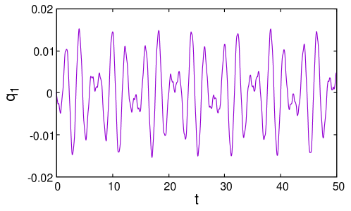
Figure 2: The displacement of the coupling point.

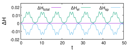
Figure 3: The energy variation of the subsystems and their sum.

The relationship between ${\mathrm{d}}u_{n_{b}}$ and ${\mathrm{d}}q_{1}$ is obtained by integrating and taking the exterior derivative of (9):

$$\frac{1}{\rho A}v_{n_{b}}-\frac{1}{m_{1}}p_{1} =C\quad(C:\mathrm{constant})$$

$$u_{n_{b}}-q_{1} =C$$

$${\mathrm{d}}u_{n_{b}}-{\mathrm{d}}q_{1} ={\mathrm{d}}C=0.$$

Hence the condition of Theorem 7

$${\mathrm{d}}f\wedge u_{n_{b}}-{\mathrm{d}}f\wedge{\mathrm{d}}q_{1}=0$$

holds, and the coupled system is symplectic.

We conducted a numerical experiment with the Sörmer–Verlet method under $L=1,N_{x}=51,b=0.2,n_{b}=10,T=50,N_{t}=10^{5},\rho=10,A=E=I=1,m_{1}=m_{2}=0.1,k=0.5$. The spatial and temporal step sizes are $\Delta x=2\times 10^{-2},\Delta t=5\times 10^{-4}$. At $t=0$, the displacements of the beam and the coupled mass $m_{1}$ are set to 0, while $q_{2}$ is set to $-1.0$.

The results are shown in Figs. 2–4. Fig. 3 shows that the energy variations from its initial values for the subsystems ($\Delta H_{\mathrm{el}}$ and $\Delta H_{\mathrm{sp}}$) are complementary to each other, and the total energy $H$ is conserved.

The symplecticity can be confirmed by the order property of the modified Hamiltonian [3] and the Sörmer-Verlet method. To check the order property of the method, we conducted additional experiments with different $\Delta t$’s under fixed $T=500$. Fig. 4 shows the results of $\Delta t=5\times 10^{-4}$ and $\Delta t=2.5\times 10^{-4}$. We can see that the variation of the total energy decreases in proportion to the square of the time step. This proportionality reflects the fact that the method preserves the modified Hamiltonian in order 1, and that the symplectic integrators are valid for the system.

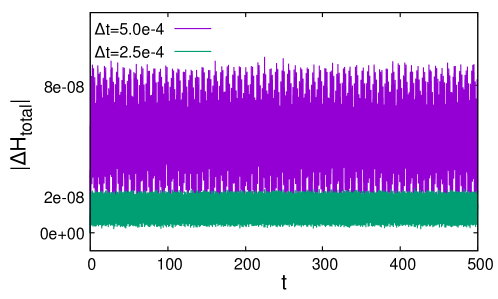
Figure 4: Variation of the total energy for different time steps. Halving the time step quarters the energy fluctuation; it shows the order property of the Sörmer-Verlet method.

7 Conclusion

We have proposed a condition under which a coupled system that consists of two Hamiltonian systems became locally a Hamiltonian system. This result enables us to check the applicability of the symplectic integrators to complicated coupled systems.

As related work, port-Hamiltonian systems, which are an extension of Hamiltonian systems, have been studied[7]. It is known that the composition of a port-Hamiltonian system is also a port-Hamiltonian system; however, port-Hamiltonian systems are formulated by focusing on the Dirac structure rather than the conservation of symplectic forms, and the applicability of symplectic integrators is not well understood. The availability of symplectic integrators for such systems should be investigated in future work.

References

- [1] J. Chabassier, P. Joly and A. Chaigne, Modeling and simulation of a grand piano, J. Acoust. Soc. Am., 134 (2013), 648–665.
- [2] E. Hairer, C. Lubich, and G. Wanner, Geometric numerical integration: structure-preserving algorithms for ordinary differential equations, Springer, Berlin, 2006.
- [3] B. Leimkuhler and S. Reich, Simulating Hamiltonian Dynamics, Cambridge University Press, Cambridge, 2005.
- [4] S. Terakawa and T. Yaguchi, Simplecticity of Coupled System of the Wave Equation and the Elastic Equation, Trans. JSIAM, 30 (2020), 269–289.
- [5] D. McDuff, D. Salamon, Introduction to Symplectic Topology, 3rd ed., Oxford University Press, Oxford, 2017.
- [6] D. Furihata and T. Matsuo, Discrete Variational Derivative Method: A Structure-Preserving Numerical Method for Partial Differential Equations, Chapman and Hall/CRC press, Florida, 2010.
- [7] V. Duindam et all., Modeling and Control of Complex Physical Systems, Springer, Berlin, 2009.