Learning Robust and Lightweight Model through Separable Structured Transformations

Abstract

With the proliferation of mobile devices and the Internet of Things, deep learning models are increasingly deployed on devices with limited computing resources and memory, and are exposed to the threat of adversarial noise. Learning deep models with both lightweight and robustness is necessary for these equipments. However, current deep learning solutions are difficult to learn a model that possesses these two properties without degrading one or the other. As is well known, the fully-connected layers contribute most of the parameters of convolutional neural networks. We perform a separable structural transformation of the fully-connected layer to reduce the parameters, where the large-scale weight matrix of the fully-connected layer is decoupled by the tensor product of several separable small-sized matrices. Note that data, such as images, no longer need to be flattened before being fed to the fully-connected layer, retaining the valuable spatial geometric information of the data. Moreover, in order to further enhance both lightweight and robustness, we propose a joint constraint of sparsity and differentiable condition number, which is imposed on these separable matrices. We evaluate the proposed approach on MLP, VGG-16 and Vision Transformer. The experimental results on datasets such as ImageNet, SVHN, CIFAR-100 and CIFAR10 show that we successfully reduce the amount of network parameters by 90%, while the robust accuracy loss is less than 1.5%, which is better than the SOTA methods based on the original fully-connected layer. Interestingly, it can achieve an overwhelming advantage even at a high compression rate, e.g., $200$ times.

1 Introduction

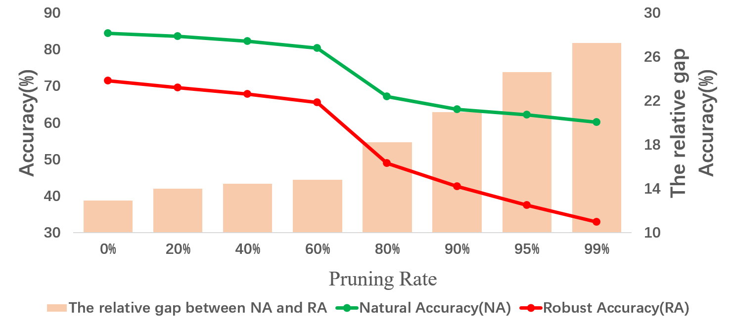
Figure 1: Natural accuracy and robust accuracy with different pruning rates. Adversarial examples are generated by the FGSM attack. This example of using ResNet-18 for classification on the CIFAR-$10$ dataset shows that pruning can reduce both NA and RA, but the drop of the latter is larger.

Despite Deep Neural Networks (DNNs) have made impressive achievements on machine learning tasks from computer vision to speech recognition and natural language processing [7, 5, 23], DNNs are vulnerable when it encounters the specially-crafted adversarial examples [16, 32, 60]. This problem provokes people to worry about the potential risk of the DNNs and attracts the researchers’ interest in the adversarial robustness of models. Current research of adversarial robustness mainly focuses on the standard DNNs, such as VGG [48], ResNet [22] and EfficientNet [51]. On the contrary, most researchers have not placed required emphasis on the robustness of lightweight networks. Lightweight DNNs are widely equipped in embedded devices due to the limitation of their computation, memory and power resources [21, 30, 63]. The vulnerability of lightweight DNNs is unacceptable and dangerous for embedded systems that need high level of robustness. For instance, the misclassification of traffic signs by self-driving cars could lead to traffic accidents. Therefore, for the embedded systems, it is necessary to construct lightweight DNN models that are robust with respect to various perturbations.

However, recent research has shown that it is challenge to achieve accuracy, lightweight, and robustness at high level simultaneously [55, 20, 69]. On the one hand, most of the existing lightweight technologies, such as pruning [21, 61] and low-rank based factorization [11, 30], tend to either decrease the rank of parameter matrix or cause an ill-conditioned matrix, which may result in the models being vulnerable to perturbations from the environment [26]. An example shown in Fig. 1 demonstrates that the more the network is pruned, the more the robust accuracy is lost. On the other hand, the strategies focused on robust training are likely to limit the success of achieving model lightweight, as deep and wide model capacities contribute to the robustness [35, 66]. With the goal of solving the natural contradiction between lightweight and robustness, this paper designs a model that is both lightweight and robust, in which the fully-connected layer is replaced by several separable transformation matrices through the Kronecker product with joint constraints. First of all, in order to reduce the parameters while avoiding the parameter matrix tends to low rank, the fully-connected layer is converted into several separable small matrices through the Kronecker product. This leads to the significant reduction in model parameters, however, the dimension of the parameter matrix of the fully-connected layer is maintained. In other words, this transformation hardly affects the expressiveness of features. Secondly, we imposed a sparsity constraint on all underlying separable small matrices. Moreover, we propose a differentiable constraint on the condition number of the parameter matrix, which structurally strengthens the robustness of the model. Finally, we incorporate the proposed separable transformations associated with joint constraints into the framework of adversarial training, with the goal of further enhancing the model robustness against imperceptible but deliberately designed adversarial noise.

2 Related Work

Adversarial Attack and Defense.

Szegedy et al. [50] first discovered that models trained on huge datasets are vulnerable to adversarial examples. Goodfellow et al. [16] explored the underlying reasons for the existence and generalisability of adversarial examples. Additionally, they presented two methods to generate adversarial examples in a white-box setting, the fast gradient method (FGM) and the fast gradient sign method (FGSM). After that, a large number of adversarial attack algorithms have been proposed, such as C&W Attack [4], DeepFool [36], the Jacobian-based Saliency Map (JSMA) [40], the Basic Iterative Method (BIM) [32], the Projected Gradient Descent attack (PGD) [35] and the structured adversarial attack [60]. Meanwhile, plenty of adversarial defense methods have also been proposed, including adversarial training [35], ensemble training [52], gradient masking [39], obfuscated gradients identification [2], adding randomness [59], replacing the output activation by an interpolating function [54, 65], using Neural Architecture Search (NAS) technology to improve model robustness [19], and defensive distillation [41, 40].

Lightweight and efficient methods.

Most lightweight networks are obtained by either compressing existing over-parameterized DNN models, called model compression, or designing small networks directly. The typical model compression techniques include pruning [21, 61], factorizing [11, 64, 30], quantizing [56, 14, 63], or distilling [24, 42] the pre-trained weights while maintaining competitive accuracy. To avoid the pre-training over-parameterized large models, one could also focus on directly building small and efficient network architectures that could be trained from scratch. For example, SqueezeNet [29] proposed lightweight CNN architectures by using smaller-sized filters, less input channels, and delayed downsampling. Many notable deep learning models such as Xception [7], MobileNet V1[27], MobileNet V2 [45], ShuffleNet [67] and CondenseNet [28] employed depthwise separable convolution. All these methods pay little attention to the robustness of lightweight models.

Robust and lightweight learning method.

Some recent works have attempted to build models that are both robust and lightweight by incorporating model compression techniques into the adversarial defense framework. Sehwag et al. [46] formulated the pruning process as an empirical risk minimization problem within adversarial loss objectives. Madaan et al. [34] proposed to suppress vulnerability by pruning the latent features with high vulnerability. Ye et al. [62] incorporated the weight pruning into the framework of adversarial training associated with min-max optimization, to enable model compression while preserving robustness. Other than weight pruning, Lin et al. [33] proposed a novel defensive quantization method by controlling the neural network’s Lipschitz constant during quantization. The authors developed in [15] distillation methods that produce robust student networks by minimizing discrepancies between the outputs of a teacher on natural images and the outputs of a student on adversarial images. Recently, Gui et al. [18] proposed a unified framework for adversarial training with pruning, factorization and quantization being the constraints. The aforementioned methods combined the model compression and adversarial defense strategies, with the main focus on achieving adversarially robust models, without addressing inherent contradictions between model compression and model robustness.

3 Learning Robust and Lightweight Transformation with Separable Structures

Most deep learning models consist of dozens levels of linear transformations and activation functions, as follows,

$$\mathbf{y}=\mathbf{W}\mathbf{x}+\bm{b},\;\;\;\mathbf{h}=\sigma(\mathbf{y})$$ (1)

where $\mathbf{x}$, $\bm{b}$, $\mathbf{W}$ being an input signal, the bias term, and the corresponding linear transformation matrix, respectively. $\mathbf{h}$ is the output response, $\sigma(\cdot)$ denotes an activation function. If $\mathbf{x}$, $\mathbf{h}$ lie in 1-dimensional (1D) tensor space, Eq. (28) covers prominent deep learning models like CNNs, RNNs and auto-encoders. For example, each row of $\mathbf{W}$ could be a reshaped convolutional filter of CNNs with $\mathbf{W}$ being a collection of matrices that contains all convolutional filters in certain layer [68]. For the fully-connected (FC) layer of CNNs or auto-encoders, $\mathbf{W}$ is a common linear transformation matrix. Generally, given a multi-dimensional (MD) input signal $\mathcal{X}$, one common way in a DNN is to reshape $\mathcal{X}$ into a 1-dimensional tensor $\mathbf{x}$ and feed it to the system Eq.(28). This may result in the loss of spatial geometry structure information and expensive computation costs when encountering high-dimensional input signal.

Learning a both robust and lightweight model, we want the system in Eq. (28) to have the following properties: i) $\mathbf{W}$ has a small amount of parameters, and its entries are sparse in a reduced data format. ii) $\mathbf{h}$ is robust to small changes around the input data, which could be achieved by learning a well-conditioned transformation $\mathbf{W}$ and preventing major changes from activation function.

To address the difficulty of a learning model in attaining both properties without degrading each other, we exploit well-conditioned matrices with small sizes that work for the system of Eq. (28). In the following, we first introduce separable structured linear transformations that have very small sizes, such that we can effectively impose the robustness and the sparsity constraints on the separable small-sized matrices.

3.1 Learning Separable Structured Transformations

We consider the general case here by assuming that the input signal is a multi-dimensional tensor. It is worth noting that the dimension of transformation is essentially limited by memory and computing resources. Consequently, the transformation is allowed to have a separable structure. In other words, the input tensor is replaced by the tensor product (a.k.a. Kronecker product) of several small-sized matrices.

In order to establish the multiplication of a higher-order signal tensor by separable matrices, we define the $n-$mode product as follows, by referring to the concept of tensor operation in [53].

Definition 1 ($n-$mode product).

The $n-$mode product of a tensor $\mathcal{X}\in\mathbb{R}^{I_{1}\times I_{2}\times\cdots\times I_{N}}$ by a matrix $\mathbf{A}\in\mathbb{R}^{K_{n}\times I_{n}}$ with $n\leq N$, is denoted by $\mathcal{X}\times_{n}\mathbf{A},$ which is an $(I_{1}\times I_{2}\times\cdots\times I_{n-1}\times K_{n}\times I_{n+1}\times\cdots\times I_{N})-$tensor. For all $k_{n}=1,\cdots,K_{n}$, the entries of the tensor $\mathcal{X}\times_{n}\mathbf{A}$ are defined as

$$(\mathcal{X}\times_{n}\mathbf{A})_{i_{1}i_{2}\cdots i_{n-1}k_{n}i_{n+1}i_{N}}=\sum_{i_{n}=1}^{I_{n}}{X_{i_{1}i_{2}\cdots i_{N}}A_{k_{n}i_{n}}}$$

with $X_{i_{1}i_{2}\cdots i_{N}}$, $A_{k_{n}i_{n}}$ being entries in $\mathcal{X}$ and $\mathbf{A}$, respectively.

Let us now refer to the linear transformation in Eq. (28). Suppose a tensor signal $\mathcal{X}\in\mathbb{R}^{I_{1}\times I_{2}\times\cdots\times I_{N}}$ is multiplied by $T$ separable transformation matrices, $\mathcal{A}:=\{\mathbf{A}^{(1)}\in\mathbb{R}^{K_{1}\times I_{1}},\mathbf{A}^{(2)}\in\mathbb{R}^{K_{2}\times I_{2}},\cdots,\mathbf{A}^{(T)}\in\mathbb{R}^{K_{T}\times I_{T}}\}$. The response $\mathcal{Y}\in\mathbb{R}^{K_{1}\times K_{2}\times\cdots\times K_{N}}$ is formulated as the $n-$mode product of $\mathcal{X}$ and these $T$ separable transformation matrices as

$$\mathcal{Y}=\mathcal{X}\times_{1}\mathbf{A}^{(1)}\times_{2}\mathbf{A}^{(2)}\times_{3}\cdots\times_{T}\mathbf{A}^{(T)}.$$ (2)

The increasing of $T$ reduces the computational load of the model, but it may degrade the expressiveness of the parameters [43, 47]. Instead, the transformation in Eq. (30) can be conveniently converted to the 1D model of (28) with a structured transformation as follows:

$$\text{vec}(\mathcal{Y})=\left(\mathbf{A}^{(1)}\otimes\mathbf{A}^{(2)}\otimes\cdots\otimes\mathbf{A}^{(T)}\right)\text{vec}(\mathcal{X}),$$ (3)

where the vector space isomorphism $\text{vec}:\mathbb{R}^{a\times b}\rightarrow\mathbb{R}^{ab}$ is defined as the operation that stacks the columns on top of each other, e.g., $\mathbf{x}=\text{vec}(\mathcal{X})$ and $\mathbf{y}=\text{vec}(\mathcal{Y})$. Therein, $\otimes$ denotes the Kronecker product operator. We refer to a large, linear transformation matrices $\mathbf{W}$ that can be represented as a concatenation of smaller matrices $\mathcal{A}:=\{\mathbf{A}^{(1)},\mathbf{A}^{(2)},\cdots,\mathbf{A}^{(T)}\}$ as a separable transformation,

$$\mathbf{W}=\mathbf{A}^{(1)}\otimes\mathbf{A}^{(2)}\otimes\cdots\otimes\mathbf{A}^{(T-1)}\otimes\mathbf{A}^{(T)},$$ (4)

with the property [17] of

$$\begin{split}\mathbf{A}^{(1)}\otimes\mathbf{A}^{(2)}\otimes\mathbf{A}^{(3)}&=(\mathbf{A}^{(1)}\otimes\mathbf{A}^{(2)})\otimes\mathbf{A}^{(3)}\\ &=\mathbf{A}^{(1)}\otimes(\mathbf{A}^{(2)}\otimes\mathbf{A}^{(3)}),\end{split}$$ (5)

$$\|\mathbf{A}^{(1)}\otimes\mathbf{A}^{(2)}\otimes\mathbf{A}^{(3)}\|=\|\mathbf{A}^{(1)}\|\|\mathbf{A}^{(2)}\|\|\mathbf{A}^{(3)}\|,$$ (6)

$$\text{rank}(\mathbf{W})=\text{rank}(\mathbf{A}^{(1)})\text{rank}(\mathbf{A}^{(2)})\cdots\text{rank}(\mathbf{A}^{(T)}).$$ (7)

As shown in Eq. (28) and Eq. (22), the overall dimension of $\mathbf{W}$ is $K_{1}\times I_{1}\times K_{2}\times I_{2}\times\cdots\times K_{T}\times I_{T}$. In comparison, $\mathcal{A}$ has a much smaller size $K_{1}\times I_{1}+K_{2}\times I_{2}+\cdots+K_{T}\times I_{T}$. In other words, the size of problem (30) is much more lightweight than the size of problem (28) given the same input signal.

3.2 Learning Robust and Lightweight Model via Separable Transformations

In this subsection, we show how to incorporate the aforementioned separable transformations of tensors into a task-specific learning model, e.g., classification, with the proposed regularizations.

Let $\mathcal{X}\in\mathbb{R}^{I_{1}\times I_{2}\times\cdots\times I_{N}}$, ${z}$ be an input tensor signal and the corresponding label, respectively. $\mathcal{X}$ together with ${z}$ follow an underlying data distribution $\mathfrak{D}$ in data space. A well-trained classifier model is a mapping $f\colon\mathcal{X}\mapsto{z}$ with a collection of separable parameters $\mathcal{A}$, denoted by ${z}=f(\mathcal{A},\mathcal{X})$. Therein, the layer of linear transformation is constructed by Eq. (30). Generally, there exists a suitable loss function $L(\mathcal{A},\mathcal{X},{z})$ to measure the risk of mapping $f$. For example, $L$ is the cross-entropy loss for a neural network $f$ [35]. The goal of the model $f$ is to find parameters $\mathcal{A}$ that minimize the risk $\mathbb{E}_{(\mathcal{X},{z})\sim\mathfrak{D}}[L(\mathcal{A},\mathcal{X},{z})]$. Furthermore, it is expected that this model is robust to perturbations and contains as few parameters as possible. To achieve this goal, the following develops several constraints that are imposed on parameters $\mathcal{A}$ defined in Eq. (30).

Considering the MD tensor operation in the model, it is difficult to directly develop constraints for the system (30). However, the mutual transformation (see Eq. (29) and Eq. (22) ) between MD model and 1D model enables solving MD transformation problem to take advantage of 1D classic and high efficient algorithms. In order to develop learning paradigms for further promoting lightweight and robustness by using separable parameters, we now derive the following propositions between the MD model and the 1D model, and hence construct appropriate regularizations.

3.2.1 Sparsity Constraint for Pruning

In order to further reduce the computational load and the complexity of separable parameters, in the following, one way is to prune the unimportant connections with small weights in training models.

Definition 2 ($s-$sparse tensor).

If a tensor $\mathcal{X}\in\mathbb{R}^{I_{1}\times I_{2}\times\cdots\times I_{N}}$ satisfies sparsity condition $\|\mathcal{X}\|_{0}\leq s,\;\mathrm{for}\;\;s\in\mathbb{Z}^{+},$ we call the tensor $\mathcal{X}$ is $s$-sparse. Here, $\|\mathcal{X}\|_{0}$ denotes the number of nonzero terms in $\mathcal{X}$.

Proposition 1.

Given $\mathbf{W}=\mathbf{A}\otimes\mathbf{B}$ with $\mathbf{W}\in\mathbb{R}^{K_{1}K_{2}\times I_{1}I_{2}}$, $\mathbf{A}\in\mathbb{R}^{K_{1}\times I_{1}}$ being $s_{\mathbf{A}}-$sparse and $\mathbf{B}\in\mathbb{R}^{K_{2}\times I_{2}}$ being $s_{\mathbf{B}}-$sparse, the sparsity of $\mathbf{W}$ is $s_{\mathbf{A}}K_{1}K_{2}+s_{\mathbf{B}}I_{1}I_{2}-s_{\mathbf{A}}s_{\mathbf{B}}$.

The model pruning is to make $T$ separable matrices $\mathcal{A}$ have few nonzero elements, while ensuring $\mathcal{A}$ without reducing expressiveness. As shown in Proposition 1, the sparsity of whole 1D system is determined by the sparsity of each separable matrix. Therefore, a natural way for pruning is to promote the sparsity of each element in $\mathcal{A}$, given by,

$$g(\mathcal{A})=\sum_{t=1}^{T}\sum_{i_{n},k_{n}}g\left(A^{(t)}_{i_{n}k_{n}}\right)$$ (8)

with $A^{(t)}_{i_{n}k_{n}}$ being an element of $\mathbf{A}^{(t)}$. For example, by appealing to the $\ell_{p}$ norm with $0<p\leq 1$, $g(\mathbf{A}^{(t)})=\|\mathbf{A}^{(t)}\|_{p}$ is used. Promoting the sparse structure of $\mathcal{A}$ helps its pruning in the training process, but it may lead to ill-conditioned matrices for $\mathcal{A}$, see Fig. 2.

Figure 2: The condition of parameter matrix becomes worse following the increase of pruning.

3.2.2 Moderate Condition Number

The condition number of $\mathbf{W}$ in Eq. (28) determines how much a small perturbation of the input $\mathbf{x}$ can change the output $\mathbf{y}$. A matrix with the condition number being close to one is said to be ”well-conditioned”, while a matrix with a large condition number is said to be “ill-conditioned”, which causes the vanishing and exploding gradient problem [10]. Both reached the limit, a unitary matrix has a condition number of $1$, while a low-rank matrix has a condition number equal to infinite. The unitary transformation may degrade the expressiveness of learning models, but the low-rank transformation is sensitive to perturbations. Therefore, the transformation with a moderate condition cumber is necessary for many linear learning models.

Definition 3 ($\ell_{2}-$norm condition number [10]).

The $\ell_{2}-$norm condition number of a full-rank matrix $\mathbf{A}\in\mathbb{R}^{K\times I}$ is defined as $\kappa(\mathbf{A})=\dfrac{\sigma_{\max}(\mathbf{A})}{\sigma_{\min}(\mathbf{A})},$ where $\sigma_{\max}(\mathbf{A})$ and $\sigma_{\min}(\mathbf{A})$ are maximal and minimal singular values of $\mathbf{A}$.

A robust linear system like Eq. (28) often requires the transformation matrix is as “well-conditioned” as possible. Considering the equal conversion between a linear tensor system (30) and its 1D version in Eq. (29), the perturbation analysis for the problem (30) can be achieved by observing the Kronecker product linear system (29) [58]. Therefore, let all separable matrices are full rank, with the properties in Eq. (23) and Eq. (24), the condition number for the Kronecker product linear system (29) associated with Kronecker decomposition (22) is deduced as

$$\kappa(\mathbf{W})=\kappa(\mathbf{A}^{(1)})\kappa(\mathbf{A}^{(2)})\cdots\kappa(\mathbf{A}^{(T)}).$$ (9)

The proof is given in Supplementary Material.

According to Eq. (24), Eq. (25) and Eq. (21), properties of the whole tensor system (30) are heavily dependent on the construction of each separable matrix $\{\mathbf{A}^{(t)}\}$. Hence, in order to improve the robustness of defined tensor system, it is necessary to approximately hold a moderate condition number for each separable matrix $\{\mathbf{A}^{(t)}\}$. According to the definition of $\ell_{2}-$norm condition number, one viable way is to develop some smooth measures to prevent singular values from being essentially small and extremely large.

Let $\{\sigma_{i}\}_{i=1}^{k},k=\min\{a,b\}$ denote the singular values of a separable matrix $\mathbf{A}^{(t)}\in\mathbb{R}^{a\times b}$ in decreasing order of magnitude, and $\sigma_{\max}(\mathbf{A}^{(t)})$ denotes the largest one. It is known that $\|\mathbf{A}^{(t)}\|_{F}^{2}={\sum_{i=1}^{k}}\sigma_{i}^{2}\geq\sigma_{\max}(\mathbf{A}^{(t)})^{2}$. Thus, imposing a penalty as in Eq. (10) could result in a small $\sigma_{\max}(\mathbf{A}^{(t)})$.

$$\leavevmode\resizebox{234.87749pt}{}{$\rho({\mathcal{A}})=\dfrac{1}{2Tk^{2}}\sum_{t=1}^{T}\|\mathbf{A}^{(t)}\|_{F}^{2}$},$$ (10)

On the other hand, $\mathbf{A}^{(t)}$ is expected to be full rank, and the Gram matrix ${\mathbf{A}^{(t)}}^{\top}\mathbf{A}^{(t)}$ is positive definite, which implies $\text{det}({\mathbf{A}^{(t)}}^{\top}\mathbf{A}^{(t)})>0$. Recalling that $\text{det}({\mathbf{A}^{(t)}}^{\top}\mathbf{A}^{(t)})=\prod\sigma_{i}^{2}$, thus the constraint term in Eq. (11) is provided to avoid the worst case of $\prod\sigma_{i}^{2}$ being exponentially small (e.g., the existence of zero or linear dependent columns/rows) and big (e.g., the existence of largely scaled columns/rows).

with $0<\nu\ll 1$ being a small smoothing parameter. Additionally, the penalty $\tau(\mathcal{A})$ also promotes the full rank of the elements in $\mathcal{A}$, i.e., $\sigma_{\min}(\mathbf{A}^{(t)})>0$, as well as the full rank of $\mathcal{A}$ in matrix-vector-product, shown in Eq. (29). Such two constraints $\rho({\mathcal{A}})$ and $\tau(\mathcal{A})$ work together to achieve a moderate condition number for the tensor system.

3.2.3 The Objective Function for RLST model

All above concepts allow us to develop learning paradigms for further promoting the lightweight and the Robustness by appealing to the classic concepts. To minimize the empirical risk $\mathbb{E}_{(\mathcal{X},{z})\sim\mathfrak{D}}[L(\mathcal{A},\mathcal{X},{z})]$, we now construct a unified cost function for the classification model $f$ to jointly learn robust and lightweight parameters with separable structures, as

$$\begin{split}\min_{\mathcal{A}}\;\big{\{}\mathbb{E}_{(\mathcal{X},{z})\sim\mathfrak{D}}[&L(\mathcal{A},\mathcal{X},{z})]+\mu_{1}\rho(\mathcal{A})\\ &+\mu_{2}\tau(\mathcal{A})+\mu_{3}g(\mathcal{A})\big{\}}\end{split}$$ (12)

where three weighting factors $\mu_{1},\mu_{2},\mu_{3}\in\mathbb{R}^{+}$ control the influence of regularizers on the final solution. In the paper, we refer to Eq. (12) as Robust and Lightweight model via Separable Transformations (RLST model).

3.3 Adversarial Training with both lightweight and Robustness

The aforementioned constraints could reduce the sensitivity of basic linear system (30) to the perturbations imposed on transformation matrices $\mathcal{A}$ and responses $\mathcal{Y}$. However, the multiple layers of linear transformation associated with nonlinear activations also suffer from hand-crafted adversarial attacks, which are implemented by adding crafted perturbations onto benign examples. In the following, we further improve the robustness of proposed RLST model by using adversarial training for tensors, which is known as an efficient learning framework against adversarially crafted attacks.

Given an input tensor signal $\mathcal{X}\in\mathbb{R}^{I_{1}\times I_{2}\times\cdots\times I_{N}}$ and corresponding label ${z}$, classification model is denoted by ${z}=f(\mathcal{A},\mathcal{X})$. The adversary’s goal is to find an adversarial example $\mathcal{X}^{adv}=\mathcal{X}+\delta$ that fools the classifier $f$, i.e., taking $\mathcal{X}+\delta$ as an input result in a much worse classification result of $f$. Therein, $\delta$ denotes a small additive perturbation. Formally, the tensor adversarial examples could be generated by the solving the following maximization problem:

$$\mathcal{X}^{adv}=\underset{\|\mathcal{X}^{adv}-\mathcal{X}\|_{p}\leq\epsilon}{\arg\max}L(\mathcal{A},\mathcal{X}^{adv},{z}),$$ (13)

where $\epsilon\in\mathbb{R}^{+}$ is a small scaling parameter, $L$ is the loss function used to train the adversarial model, e.g., cross-entropy for a neural network [35], and $\|\cdot\|_{p}$ with $p\geq 0$ denotes the $\ell_{p}$ norm of a tensor, which is used to measure the distance between $\mathcal{X}^{adv}$ and $\mathcal{X}$. The goal of tensor adversarial training against adversarial examples $\mathcal{X}^{adv}$ is to find model parameters $\mathcal{A}$ via optimizing the following min-max Empirical risk problem

$$\min_{\mathcal{A}}\;{\mathbb{E}_{(\mathcal{X},{z})\sim\mathfrak{D}}\underset{\|\mathcal{X}^{adv}-\mathcal{X}\|_{p}\leq\epsilon}{\arg\max}L(\mathcal{A},\mathcal{X}^{adv},{z})},$$ (14)

where $\mathfrak{D}$ denotes the underlying training data distribution.

Algorithm 1 :Algorithm for ARLST function

1:  Input: Training set $\mathcal{D}$, iterations $K$, model $f_{\mathcal{A}}$ with separable parameters $\mathcal{A}$, batch size $T$, $\mu_{1},\mu_{2},\mu_{3}$, attacks

2:  Output: parameters $\mathcal{A}$

3:  for $i\;=\;1\;to\;\textit{K}$ do

4:     Read mini-batch $\mathcal{X}\subset\mathcal{D}$

5:     Given $\mathcal{A}$, generate $T$ adversarial examples $\mathcal{X}^{adv}:=\{\mathcal{X}^{adv}_{1},\cdots,\mathcal{X}^{adv}_{T}\}$ from corresponding clean signals $\mathcal{X}$ by solving the inner max in Eq. (15)

6:     Apply Adam optimizer on the outer min in Eq. (15), to update $\mathcal{A}$ by using learned $\mathcal{X}^{adv}$

7:  end for

By combining the regularizers discussed above, we construct the following cost function to jointly learn robust and lightweight parameters with separable structures, as

$$\begin{split}\min_{\mathcal{A}}\;\big{\{}&\mathbb{E}_{(\mathcal{X},{z})\sim\mathfrak{D}}\underset{\|\mathcal{X}^{adv}-\mathcal{X}\|_{p}\leq\epsilon}{\arg\max}L(\mathcal{A},\mathcal{X}^{adv},{z})\\ &+\mu_{1}\rho(\mathcal{A})+\mu_{2}\tau(\mathcal{A})+\mu_{3}g(\mathcal{A})\big{\}}\end{split}$$ (15)

with $\mu_{1},\mu_{2},\mu_{3}\in\mathbb{R}^{+}$. In this work, we refer to it as the Adversarial RLST (ARLST) function.

The gradients

The key requirement for developing a gradient algorithm to optimize the cost function Eq. (12) or Eq. (15), is the differentiability of LRST/ALRST function w.r.t. $\mathcal{A}$. By taking ALRST as an example, let ${J}$ and $\mathbf{A}$ denote by the cost function in Eq. (15) and one of its separable parameter, the Euclidean gradient $\nabla{J}(\mathbf{A})$ is computed as

$$\begin{split}\nabla{J}(\mathbf{A})=&\nabla_{L}(\mathbf{A})+\mu_{1}\nabla_{\rho}(\mathbf{A})+\mu_{2}\nabla_{\tau}(\mathbf{A})\\ &+\mu_{3}\nabla_{g}(\mathbf{A}).\end{split}$$ (16)

Since the optimization on DNNs is nowadays well established, $\nabla_{L}(\mathbf{A})$ is commonly available and its Euclidean gradient depends on the DNN architectures of use [22, 25]. In Eq. (16), it has

$$\nabla_{{\rho}}(\mathbf{A}) =\dfrac{1}{k^{2}}\mathbf{A},$$ (17)

$$\nabla_{\tau}(\mathbf{A}) =\dfrac{\eta}{\log(k)}\mathbf{A}(\eta\mathbf{A}^{\top}\mathbf{A})^{-1}.$$

Here, we enforce the sparsity of $\mathbf{A}$ by minimizing a $\ell_{p}$ norm with $0\leq p\leq 1$. In practice, we use the following penalty term to constrain $\mathbf{A}$ instead of Eq. (8) ,

$$g(\mathbf{A})=\frac{1}{2k_{1}}\sum_{i=1}^{k_{1}}(\frac{1}{p}\|\mathbf{a}_{i,:}\|_{p}^{p})^{2},$$ (18)

with $\mathbf{a}_{i,:}$ being the $i^{\text{th}}$ row of $\mathbf{A}$. However, it is known that above $\ell_{p}$ norm is non-smooth. In order to make the global cost function differentiable, we exchange Eq. (18) with a smooth approximation that is concretely given as

$$g(\mathbf{A})=\frac{1}{2k_{1}}\sum_{i=1}^{k_{1}}(\sum_{j=1}^{k_{2}}(\mathbf{a}_{ij}^{2}+\varpi)^{{p}/{2}})^{2},$$ (19)

with $0<\varpi<1$ being a smoothing parameter. Then, the Euclidean gradient $\nabla_{g}(\mathbf{A})$ is computed as

$$\nabla_{g}(\mathbf{A})=\dfrac{1}{k_{1}}\sum_{i=1}^{k_{1}}\dfrac{1}{p}\sum_{j=1}^{k_{2}}(\mathbf{a}_{ij}^{2}+\varpi)^{\dfrac{p}{2}}\sum_{j=1}^{k_{2}}(\mathbf{a}_{ij}(\mathbf{a}_{ij}^{2}+\varpi)^{\dfrac{p}{2}-1}\mathbf{E}_{ij})$$ (20)

By $\mathbf{E}_{ij}$, we denote a matrix whose $i^{th}$ entry in the $j^{th}$ column is equal to one, and all the rests are zero.

With the differentiability of the RLST/ARLST function, smooth solvers, such as stochastic gradient descent algorithms, can be used for optimization. A generic framework of our ARLST algorithm is summarized in Algorithm 1.

Table 1: Comparison between a MLP and its variants.

		MLP	MLP-HYDRA	MLP-ADMM	MLP-ATMC	MLP-RLST
MNIST	Parameters	322M	5.25M($61\times$)	5.25M($61\times$)	5.25M($61\times$)	5.25M($61\times$)
	Accuracy	97.99%	74.48%	92.90%	95.83%	97.99%
CIFAR-$10$	Parameters	834.5M	14.5M($57\times$)	14.5M($57\times$)	14.5M($57\times$)	14.5M($57\times$)
	Accuracy	56.42%	47.54%	37.97%	52.42%	67.82%

4 Experimental Evaluations

In this section, we investigate the performance of the proposed RLST/ARLST function from two aspects: the size of model parameters and the model robustness against different perturbations. For the convenience of referencing, we adopt the following way to name the algorithms for comparison: for example, the VGG-$16$ [48] under the framework of the ARLST algorithm is referred to as the VGG$16$-ARLST.

Table 2: Comparison between a VGG-16 and its variants under adversarial training with PGD attack.

		VGG16-HYDRA	VGG16-ADMM	VGG16-ATMC	VGG16-ARLST
	Cr	NA/RA (Var)	NA/RA (Var)	NA/RA (Var)	NA/RA (Var)
CIFAR-10	$1\times$(pretrain, NAT)	$96.1/3.5$	$96.1/3.5$	$96.1/3.5$	$96.1/3.5$
	$1\times$(pretrain, AT)	$77.7/47.7(0.52/0.13)$	$76.0/44.8(0.25/0.16)$	$76.9/45.5(0.21/0.11)$	$\textbf{77.8/47.7}(0.29/0.10)$
	$10\times$	$75.7/46.2(0.25/0.16)$	$75.9/44.8(0.20/0.36)$	$75.6/44.8(0.18/0.19)$	$\textbf{76.6/46.3}(0.18/0.03)$
	$20\times$	$74.5/44.9(0.15/0.05)$	$74.7/43.7(0.15/0.06)$	$73.9/42.9(0.13/0.20)$	$\textbf{75.8/45.6}(0.11/0.01)$
	$100\times$	$69.8/40.2(0.09/0.26)$	$68.8/40.4(0.20/0.63)$	$69.8/41.1(0.12/0.19)$	$\textbf{70.0/41.3}(0.05/0.15)$
	$200\times$	$62.4/35.5(0.23/0.16)$	$60.6/30.5(0.05/0.32)$	$64.0/36.1(0.19/0.35)$	$\textbf{64.3/37.5}(0.02/0.09)$
SVHN	$1\times$(pretrain, NAT)	$96.2/1.2$	$96.2/1.2$	$96.2/1.2$	$96.2/1.2$
	$1\times$(pretrain, AT)	$90.5/53.5(0.35/0.23)$	$89.7/52.3(0.20/0.09)$	$90.2/52.2(0.23/0.06)$	$\textbf{90.6/53.9}(0.10/0.01)$
	$10\times$	$89.2/52.4(0.20/0.29)$	$88.2/51.6(0.32/0.19)$	$88.6/51.7(0.32/0.15)$	$\textbf{89.6/52.9}(0.08/0.05)$
	$20\times$	$85.5/51.7(0.23/0.32)$	$85.1/50.9(0.20/0.16)$	$85.4/50.8(0.11/0.20)$	$\textbf{87.5/52.8}(0.11/0.12)$
	$100\times$	$84.3/46.8(0.22/0.19)$	$83.9/45.6(0.32/0.09)$	$80.5/46.8(0.25/0.10)$	$\textbf{84.6/51.6}(0.23/0.05)$
	$200\times$	$32.9/23.1(0.10/0.26)$	$30.1/22.5(0.12/0.32)$	$70.0/30.7(0.10/0.20)$	$\textbf{73.1/34.7}(0.05/0.10)$

Datasets.

Our method is validated by experiments on image datasets, such as SVHN [37],Yale-B, MNIST, CIFAR-$10$ [31], CIFAR-$100$ [31] and ImageNet (ILSVRC2012) [44].

Implementation Settings.

We report the model performance on robustness under the FGSM attack [16], the PGD attack [35], the AutoAttack (AA) [9] and the Square Attack (SA) [1]. The PGD attack is known as the strong first-order attack. The AA is an ensemble of complementary attacks which combine new versions of PGD with some other attacks. The SA is a black-box attack, which is an adversary attack without any internal knowledge of the targeted network. Unless otherwise specified, we set the PGD attack and the AA attack with the perturbation magnitude $\epsilon=0.031$, the attack iteration numbers $n=10$, and the attack step size $s=0.0078$. We also set the number of queries in SA as 100, the perturbation magnitude of FGSM $\epsilon=0.015$.

We evaluate the model performance by using the following metrics, as i) Compression ratio (Cr): the division of regular model size by lightweight model size; ii) Natural Accuracy (NA): the accuracy on classifying benign images; iii) Robustness Accuracy (RA): the accuracy on classifying images corrupted by adversarial attack; iv) Var: the variance of accuracy results from multiple experiments. In addition, AT denotes the Adversarial Training method defined in [66] and NAT denotes the results under natural training, i.e., evaluating a learning model without adversarial training with respect to specific known attack.

Three well-known and most related methods, ADMM [62], ATMC [18], and HYDRA [46], are used for the comparison.

All networks are trained with 100 epochs for all experiments in this paper, and they are conducted on NVIDIA RTX $2080Ti$ GPU ($10$ GB memory for each GPU). Unless otherwise specified, the results of all tables are presented in percent.

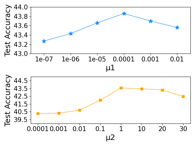
Figure 3: Impact of condition number regularization operator on test accuracy.

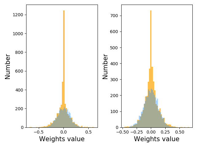
Figure 4: Distribution of parameters of two separable matrices with (yellow part) and without (dark part) sparse regularization.

Weighing the Regularisers.

Training an ARLST model is usually computationally expensive. Here, we investigate the impact of the three regularizers $\rho$, $\tau$ and $g$ on the performance of the ARLST under the PGD attack, on the CIFAR-$10$ dataset, i.e., the inference of weighing parameters $\mu_{1}$, $\mu_{2}$ and $\mu_{3}$ in Eq. (12) and Eq. (15).

We first investigate the impact of $\mu_{1}$ and $\mu_{2}$, i.e., $\rho$ and $\tau$, as shown in the Fig. 3. We set $\mu_{2}=0$, $\mu_{3}=0$ when $\rho$ is investigated, and $\mu_{1}=0$, $\mu_{3}=0$ for investigating $\tau$. Experimental results show that suitable choices of $\mu_{1}$ and $\mu_{2}$ can improve the performance of the ARLST method. $\mu_{1}=0.0001$ and $\mu_{2}=1$ achieve the superior performance.

Similarly, Fig. 4 shows that the regularizer $g$ can make the parameters more sparse and improve the lightweight of the model.

4.1 MLPs

In order to initially evaluate the performance on improving the model lightweight by RLST, a simple MLP with three layers is tested on MNIST and CIFAR-$10$, in the framework of RLST, with $T=2$, namely, MLP-RLST. For comparison, the MLP is also compressed by using ADMM, ATMC and HYDRA with the setting of NAT, namely, MLP-ADMM, MLP-ATMC and MLP-HYDRA.

As shown in Table. 1, MLP-RLST can reduce the model parameters of a MLP by more than $61\times$ on MNIST, and more than $57\times$ on CIFAR-$10$, while ensuring the same even better classification results in comparison of MLP. These results are much better than other methods, with the similar compression ratio. This indicates that MLP-RLST has more power on feature expressiveness when encountering a very high compression ratio. It is worth noting that on the CIFAR-10 dataset, MLP-RLST even outperforms the accuracy of MLP, which may be due to the fact that the former has less risk of overfitting.

Table 3: Comparison between a Vision Transformer and its variants under adversarial training with FGSM attack.

		ViT-HYDRA	ViT-ADMM	ViT-ATMC	ViT-ARLST
	Cr	NA/RA (Var)	NA/RA (Var)	NA/RA (Var)	NA/RA (Var)
MNIST	$1\times$(pretrain,NAT)	$99.47/6.41(0.32/0.20)$	$99.47/6.41(0.32/0.20)$	$99.47/6.41(0.32/0.20)$	$99.47/6.41(0.32/0.20)$
	$1\times$(pretrain,AT)	$97.32/89.86(0.25/0.22)$	$96.98/89.21(0.40/0.19)$	$97.58/90.12(0.15/0.09)$	$\textbf{97.98/90.94}(0.20/0.10)$
	$3\times$(AT)	$92.60/81.12(0.31/0.23)$	$91.98/81.08(0.23/0.31)$	$94.30/83.34(0.25/0.16)$	$\textbf{94.65/83.96}(0.21/0.15)$
Yale-B	$1\times$(pretrain,NAT)	$99.74/0.79(0.33/0.15)$	$99.74/0.79(0.33/0.15)$	$99.74/0.79(0.33/0.15)$	$99.74/0.79(0.33/0.15)$
	$1\times$(pretrain,AT)	$95.96/90.88(0.31/0.23)$	$95.20/90.10(0.19/0.22)$	$96.50/91.03(0.29/0.20)$	$\textbf{96.65/92.93}(0.10/0.25)$
	$3\times$(AT)	$93.68/89.86(0.10/0.20)$	$93.35/89.05(0.25/0.32)$	$94.65/90.89(0.23/0.53)$	$\textbf{95.83/92.74}(0.15/0.13)$

4.2 ARLST with Adversarial Training

In order to evaluate both the robustness and the lightweight of proposed ARLST model, the NA, the RA, as well as the amount of model parameters, are considered for comparison with SOTA methods, ATMC, ADMM and HYDRA. We follow their basic settings without much post processing. By taking VGG-$16$ performed on CIFAR-$10$ dataset as an example, we follow its basic architecture and construct VGG-$16$-ARLST network.

As shown in Table. 2, by using the same pre-trained setting, VGG-$16$-ARLST outperforms ATMC, ADMM and HYDRA in two datasets under different levels of compression ratio. It is worth noting that the VGG-$16$-ARLST achieves overwhelming advantage when the compression ratio is very high, e.g., $200$ times. Additionally, the VGG-$16$-ARLST has a smaller variance of the accuracies for five runs in the experiments. These results suggest that the VGG-$16$-ARLST has higher stability than above SOTA methods.

By taking the experimental results on SVHN as an example, the RA of the VGG-$16$-ARLST achieves $0.4\%$, $0.5\%$, $1.1\%$, $4.8\%$ and $11.6\%$ higher than that of HYDRA, with the compression ratio as $1\times$, $10\times$, $20\times$, $100\times$ and $200\times$, respectively. It is apparent that the VGG-$16$-ARLST achieves more advantages as the compression ratio increases. This advantage may be traced to the joint optimization of the pruning and the condition number constraint, which prevents the parameter matrix from being very ill-conditioned.

In previous experiments, we tested ARLST and other baselines against the PGD attack at certain fixed perturbation levels. Besides, we also tested all models against the FGSM attack, the Square Attack (SA) and the AutoAttack (AA) on CIFAR-$100$ dataset when the compression rate is $100\times$. Table. 4 shows the advantages achieved by ARLST. Table. 5 gives an simple comparison to show the better performance of ARLST on ImageNet.

Table 4: Comparison between a VGG-16 and its variants on CIFAR-$100$ under adversarial training with $4$ attacks.

	HYDRA	ADMM	ATMC	ARLST
Attacks	NA/RA	NA/RA	NA/RA	NA/RA
FGSM	$44.9/29.7$	$41.1/27.7$	$46.2/31.5$	47.1/32.1
PGD	$33.3/19.9$	$32.2/17.7$	$36.6/21.3$	37.6/22.1
SA	$43.0/31.7$	$41.9/30.3$	$42.9/33.6$	44.1/34.7
AA	$31.9/17.7$	$30.9/16.9$	$35.0/19.9$	35.2/20.8

Table 5: Comparison between a VGG-16 and its variants on ImageNet-1K under adversarial training with FGSM attack.

	HYDRA	ADMM	ATMC	ARLST
Cr	NA/RA	NA/RA	NA/RA	NA/RA
$5\times$	$43.2/28.7$	$41.2/27.9$	$45.1/29.5$	45.4/30.0
$10\times$	$41.6/27.0$	$40.1/26.0$	$42.9/27.8$	43.9/28.7

4.3 Vision Transformer

To our best knowledge, there have been few existing studies on examining the robustness and Lightweight of ViT [13]. Because ViT model training and adversarial training are very time-consuming, we conduct a simple set of experiments based on ViT-B/16, comparing our method with HYDRA, ADMM, and ATMC on small datasets, Yale$-B$ and MNIST. For adversarial training of ViT, we apply the FGSM attack to generate adversarial samples. We set the perturbation magnitude to be 0.3 for MNIST and 0.03 for Yale$-$B. We train four models for 100, 300 epochs on MNIST and Yale$-$B, respectively.

As shown in Table. 3, when the compression ratio is $3\times$, ARLST achieves better performance. This is because we have reduced the parameters of the FC layer and fully retained the Self-Attention, such that the performance of the model is not severely damaged.

5 Conclusions

This work proposes a learning model with the properties of both lightweight and robustness. We approximate the weight matrix of each linear layer by the tensor product of several separable structured small-sized matrices. Furthermore, we propose a joint constraint of sparsity and differentiable condition number which is imposed on these separable matrices, with the goal of promoting both the lightweight and the robustness of the whole system. We conduct min-max adversarial training based on several models combined with the proposed method, namely ARLST, to defend against adversarial attacks. The experimental results of MLP, VGG-16 and ViT show that ARLST outperforms the SOTA method based on the original fully-connected layers, achieving higher robustness to various adversarial perturbations while having fewer network parameters and less risk of overfitting. Moreover, the proposed ARLST model is flexible and can be extended to other cases of deep learning models, such as the attention module and the graph neural networks.

Appendix A Notations and Definitions

In the submitted manuscript and supplementary material, vectors, matrices, tensors are denoted by bold lower case letters $\mathbf{v}$, bold upper case ones $\bm{V}$, and mathcal letter ${\mathcal{V}}$, respectively. $\mathbf{v}\in\mathbb{R}^{ab}$ denotes a vector $\mathbf{v}$ with the dimension $ab$. $\mathbf{V}\in\mathbb{R}^{a\times b}$ denotes a matrix $\mathbf{V}$ with the resolution $a\times b$. ${V}_{i}$, ${V}_{ij}$, ${V}_{i_{1}i_{2}\cdots i_{T}}$ denotes the $i^{th}$ column of matrix $\mathbf{V}$, the entry in the $i^{th}$ row and the $j^{th}$ column of $\mathbf{V}$, the entry in a tensor ${\mathcal{V}}$ with indices $i_{j}$ indicating the position in the respective mode.

Appendix B Proof of Eq. (9) in the Submitted Manuscript

In the submitted manuscript, the Eq. (9) is shown as the following Eq. (21)

$$\kappa(\mathbf{W})=\kappa(\mathbf{A}^{(1)})\kappa(\mathbf{A}^{(2)})\cdots\kappa(\mathbf{A}^{(T)}).$$ (21)

Before the proof, we refer to a large, structured transformation matrices $\mathbf{W}$ that can be represented as a concatenation of smaller matrices $\mathcal{A}:=\{\mathbf{A}^{(1)},\mathbf{A}^{(2)},\cdots,\mathbf{A}^{(T)}\}$ as a separable transformation,

$$\mathbf{W}=\mathbf{A}^{(1)}\otimes\mathbf{A}^{(2)}\otimes\cdots\otimes\mathbf{A}^{(T-1)}\otimes\mathbf{A}^{(T)},$$ (22)

with the properties [17] of

$$\begin{split}\mathbf{A}^{(1)}\otimes\mathbf{A}^{(2)}\otimes\mathbf{A}^{(3)}&=(\mathbf{A}^{(1)}\otimes\mathbf{A}^{(2)})\otimes\mathbf{A}^{(3)}\\ &=\mathbf{A}^{(1)}\otimes(\mathbf{A}^{(2)}\otimes\mathbf{A}^{(3)}),\end{split}$$ (23)

$$\|\mathbf{A}^{(1)}\otimes\mathbf{A}^{(2)}\otimes\mathbf{A}^{(3)}\|=\|\mathbf{A}^{(1)}\|\|\mathbf{A}^{(2)}\|\|\mathbf{A}^{(3)}\|,$$ (24)

and

$$\text{rank}(\mathbf{W})=\text{rank}(\mathbf{A}^{(1)})\text{rank}(\mathbf{A}^{(2)})\cdots\text{rank}(\mathbf{A}^{(T)}).$$ (25)

Theorem 1 (Theorem $4.2.15$ in [26]).

Let $\mathbf{A}\in\mathbb{R}^{a\times b}$, $\mathbf{B}\in\mathbb{R}^{c\times d}$ have rank $\text{rank}(\mathbf{A})$, $\text{rank}(\mathbf{B})$, and let $\mathbf{V}_{\mathbf{A}},\mathbf{W}_{\mathbf{A}},\bf{\Sigma}_{\mathbf{A}},\mathbf{V}_{\mathbf{B}},\mathbf{W}_{\mathbf{B}},\bf{\Sigma}_{\mathbf{B}},$ be the matrices corresponding to their singular value decompositions. Then we can easily derive the singular value decomposition of their Kronecker product:

$$\begin{split}\mathbf{A}\otimes\mathbf{B}&=(\mathbf{V}_{\mathbf{A}}\bf{\Sigma}_{\mathbf{A}}\mathbf{W}_{\mathbf{A}}^{\top})\otimes(\mathbf{V}_{\mathbf{B}}\bf{\Sigma}_{\mathbf{B}}\mathbf{W}_{\mathbf{B}}^{\top})\\ &=(\mathbf{V}_{\mathbf{A}}\otimes\mathbf{V}_{\mathbf{B}})(\bf{\Sigma}_{\mathbf{A}}\otimes\bf{\Sigma}_{\mathbf{B}})(\mathbf{W}_{\mathbf{A}}\otimes\mathbf{W}_{\mathbf{B}})^{\top}.\end{split}$$ (26)

In Eq. (26), the singular values of $\mathbf{V}_{\mathbf{A}},\mathbf{W}_{\mathbf{A}},\mathbf{V}_{\mathbf{B}},\mathbf{W}_{\mathbf{B}}$ are equal to $1$. $\bf{\Sigma}_{\mathbf{A}}$ and $\bf{\Sigma}_{\mathbf{B}}$ are diagonal and contain the singular values of $\mathbf{A}$ and $\mathbf{B}$. The condition number of $\mathbf{A}\otimes\mathbf{B}$ could be rewritten as

$$k(\mathbf{A}\otimes\mathbf{B}) =k((\mathbf{V}_{\mathbf{A}}\otimes\mathbf{V}_{\mathbf{B}})(\bf{\Sigma}_{\mathbf{A}}\otimes\bf{\Sigma}_{\mathbf{B}})(\mathbf{W}_{\mathbf{A}}\otimes\mathbf{W}_{\mathbf{B}}))$$

$$=k(\mathbf{V}_{\mathbf{A}}\otimes\mathbf{V}_{\mathbf{B}})k(\bf{\Sigma}_{\mathbf{A}}\otimes\bf{\Sigma}_{\mathbf{B}})k(\mathbf{W}_{\mathbf{A}}\otimes\mathbf{W}_{\mathbf{B}})$$

$$=k(\bf{\Sigma}_{\mathbf{A}}\otimes\bf{\Sigma}_{\mathbf{B}})$$

$$=\dfrac{\sigma_{\max}(\bf{\Sigma}_{\mathbf{A}})\sigma_{\max}(\bf{\Sigma}_{\mathbf{B}})}{\sigma_{\min}(\bf{\Sigma}_{\mathbf{A}})\sigma_{\min}(\bf{\Sigma}_{\mathbf{B}})}$$

$$=k(\mathbf{A})k(\mathbf{B})$$

Recalling the property in Eq. (23), it is easy to conclude the Eq. (21) if Eq. (22) holds.

Appendix C A 2D Example

In the following, the problem (28) could be easily rewritten into the large-scale form of Eq. (29). For example, by regarding $\mathbf{x}\in\mathbb{R}^{m}$, $\mathbf{y}\in\mathbb{R}^{d}$, $\mathbf{W}\in\mathbb{R}^{d\times m}$ in Eq. (28), its two-dimensional system with separable structured transformations can be rewritten as

$$\mathbf{Y}=\mathbf{A}\mathbf{X}\mathbf{B}^{\top},$$ (27)

$$\mathbf{y}=\mathbf{W}\mathbf{x},\;\;\;\mathbf{h}=\sigma(\mathbf{y})$$ (28)

$$\text{vec}(\mathcal{Y})=\left(\mathbf{A}^{(1)}\otimes\mathbf{A}^{(2)}\otimes\cdots\otimes\mathbf{A}^{(T-1)}\otimes\mathbf{A}^{(T)}\right)\text{vec}(\mathcal{X}),$$ (29)

$$\mathcal{Y}=\mathcal{X}\times_{1}\mathbf{A}^{(1)}\times_{2}\mathbf{A}^{(2)}\times_{3}\cdots\times_{T}\mathbf{A}^{(T)}.$$ (30)

where $\mathbf{A}\in\mathbb{R}^{K_{1}\times I_{1}}$ and $\mathbf{B}\in\mathbb{R}^{K_{2}\times I_{2}}$ have smaller $I_{1}$ and $I_{2}$. $\mathbf{X}\in\mathbb{R}^{I_{1}\times I_{2}}$ and $\mathbf{Y}\in\mathbb{R}^{K_{1}\times K_{2}}$ are reshaped two-dimensional matrices from $\mathbf{x}$ and $\mathbf{y}$. If we read $\mathbf{W}=\mathbf{A}\otimes\mathbf{B}$ with $K_{1}K_{2}=d$ and $I_{1}I_{2}=m$, the dimension of the problem is reduced from $K_{1}K_{2}I_{1}I_{2}$ in Eq. (28) to $K_{1}I_{1}+K_{2}I_{2}$ in Eq. (27). The ratio of the parameters of two models is computed by $\eta_{1}=\frac{1}{K_{1}I_{1}}+\frac{1}{K_{2}I_{2}}$. The latter is much smaller than the former following the increase of $K_{1}I_{1}$ and $K_{2}I_{2}$.

Considering the matrix multiplication in Eq. (27), the computational complexity is also significantly reduced from $\mathcal{O}(\mathbf{W}\mathbf{x})=\mathcal{O}(K_{1}\times I_{1}\times I_{2}\times K_{2})$ to $\mathcal{O}(\mathbf{A}\mathbf{X}\mathbf{B}^{\top})=\mathcal{O}(K_{1}\times I_{1}\times I_{2}+K_{1}\times I_{2}\times K_{2})$, and the ratio of them is computed as $\eta_{2}=\frac{1}{K_{2}}+\frac{1}{I_{1}}$. The reduction of computational complexity depends on the sizes of $\mathbf{X}$ and $\mathbf{Y}$, i.e., $I_{1}$ of $\mathbf{X}$ and $K_{2}$ of $\mathbf{Y}$ with $d,m$ being fixed.

Eq. (30) shows that the number of parameters $\mathcal{A}$ and its computational complexity depend on the size of input tensor $\mathcal{X}$ and the size of output tensor $\mathcal{Y}$. The constructions of $\mathcal{X}$ and $\mathcal{Y}$ determine the structure of $\mathcal{A}$ and the computational load.

Appendix D ARLST with Adversarial Training

In the submitted manuscrip, VGG-$16$-ARLST outperforms ATMC, ADMM and HYDRA in CIFAR-10 and SVHN dataset under different levels of compression ratio. As shown in Table 6, by using the same pre-trained setting, VGG-$16$-ARLST outperforms ATMC, ADMM and HYDRA in CIFAR-10 datasets under adversarial training with FGSM attack. It is worth noting that the VGG-$16$-ARLST achieves overwhelming advantage when the compression ratio is very high, e.g., $100$ times. Additionally, the VGG-$16$-ARLST has a smaller variance of the accuracies for five runs in the experiments. These results suggest that the VGG-$16$-ARLST has higher stability than above SOTA methods.

Table 6: Comparison between a VGG-16 and its variants under adversarial training with FGSM attack.

		VGG16-HYDRA	VGG16-ADMM	VGG16-ATMC	VGG16-ARLST
	Cr	NA/RA (Var)	NA/RA(Var)	NA/RA(Var)	NA/RA(Var)
CIFAR-10	$1\times$(pretrain, NAT)	$96.2/22.4$	$96.2/22.4$	$96.2/22.4$	$96.2/22.4$
	$1\times$(pretrain, AT)	$84.1/69.4(0.23/0.15)$	$82.3/64.5(0.40/0.25)$	$83.2/64.1(0.22/0.09)$	$\textbf{85.2/70.4}(0.28/0.12)$
	$10\times$	$81.3/67.1(0.18/0.50)$	$81.1/61.6(0.22/0.32)$	$80.5/60.8(0.29/0.20)$	$\textbf{83.8/69.8}(0.23/0.20)$
	$20\times$	$81.2/66.5(0.25/0.33)$	$78.5/59.9(0.20/0.35)$	$78.9/59.7(0.19/0.25)$	$\textbf{82.6/68.4}(0.10/0.12)$
	$100\times$	$69.9/53.5(0.25/0.35)$	$65.3/48.9(0.23/0.34)$	$66.1/50.0(0.32/0.15)$	$\textbf{74.5/58.3}(0.12/0.09)$
	$200\times$	$45.1/37.4(0.19/0.20)$	$20.5/10.3(0.35/0.46)$	$61.9/43.2(0.29/0.25)$	$\textbf{63.9/49.1)}(0.20/0.12$

Appendix E The Application in CNNs

In this section, we construct the RLST function and the ARLST function for learning robust and lightweight models for classic CNNs. The following two parts in a common CNN can be modified by the proposed operator defined in Eq. (2) of the Submitted Manuscript.

The FC layers

In most CNNs, the input before flatten is often a $3$D $(\text{height, width, number of filters})$ tensor, and the Flatten operator reshapes the $3$D tensor to have a shape that is equal to the number of elements contained in the tensor. Differently, the proposed tensor operator can directly operate the $3$D input tensor and remove the Flatten layer. Hence, all classical FC layers become the tensor multiplication as shown in Eq. (2) of the Submitted Manuscript. It is worth noticing that the proposed operation is adapted to the structures of input tensor without flattening, which is different to the work in [57]. The latter used Kronecker product decomposition to approximate huge FC weight matrices after flatten layer. The similar methods based on Kronecker tensor decomposition are also shown in [8, 3, 6, 38]. The computation for tensor decomposition is expensive when processing high-dimensional signals.

By taking ZF$-5$ as an example performed on Extended Yale$-$B dataset, we follow its basic architecture and construct ARLST-ZF$-5$ network. The input before flatten is a $3$D tensor with the size of $7\times 7\times 64$. We then remove the flatten layer of ZF$-5$ and reshape the $3$D tensor as $49\times 64$. Thus, each following FC layer could be constructed by two separable transformations, i.e., $T=2$ in Eq. (2) of the Submitted Manuscript, and details are shown in Eq. (6) of the Submitted Manuscript. For example, in the FC1 layer, ARLST-ZF$-5$ uses $\mathbf{A}^{(1)}\in\mathbb{R}^{64\times 49}$ and $\mathbf{A}^{(2)}\in\mathbb{R}^{64\times 64}$, to replace a $\mathbb{R}^{3136\times 1024}$ transformation in original ZF$-5$ network. Hence, in the FC2 layer, ARLST-ZF$-5$ uses two $\mathbb{R}^{64\times 64}$ matrices to replace a $\mathbb{R}^{1024\times 1024}$ transformation in original ZF$-5$ network. Finally, ARLST-ZF$-5$ uses $\mathbf{A}^{(1)}\in\mathbb{R}^{1\times 64}$ and $\mathbf{A}^{(2)}\in\mathbb{R}^{38\times 64}$ to project the tensor to a $38-$dimensional vector, by replacing a $\mathbb{R}^{1024\times 38}$ transformation in original ZF$-5$ network. The three FC layers of ZF$-5$ have $14,534,294$ parameters, but ARLST-ZF$-5$ only has $259,606$ parameters, and $98.21\%$ parameters have been reduced.

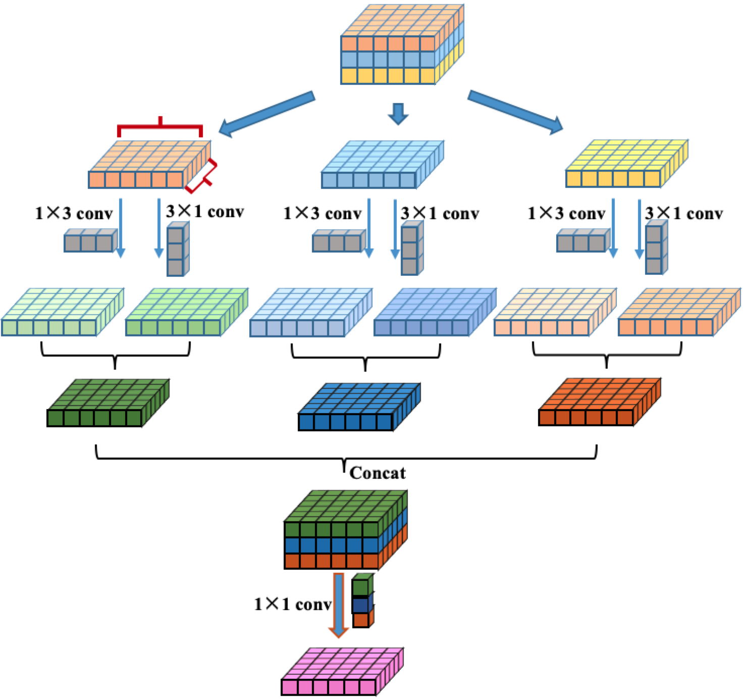
Figure 5: This figure depicts a way for constructing the convolution layer by using separable transformations.

Table 7: Network structure of convolution layers.

ID	Filter size	Num	Strides	$Act$
Conv1-1	[3,1][1,3]	16	(1,1)	—-
Conv1-2	[1,1]	16	(1,1)	ReLu
Conv2-1	[3,1][1,3]	16	(1,1)	—-
Conv2-2	[1,1]	16	(1,1)	ReLu
Pool3	[2,2]	–	(2,2)	–
Conv4-1	[3,1][1,3]	32	(1,1)	—-
Conv4-2	[1,1]	32	(1,1)	ReLu
Conv5-1	[3,1][1,3]	32	(1,1)	—-
Conv5-2	[1,1]	32	(1,1)	ReLu
Pool6	[2,2]	–	(2,2)	–
Conv7-1	[3,1][1,3]	64	(1,1)	—-
Conv7-2	[1,1]	64	(1,1)	ReLu
Conv8-1	[3,1][1,3]	64	(1,1)	—-
Conv8-2	[1,1]	64	(1,1)	ReLu
Conv9-1	[3,1][1,3]	64	(1,1)	—-
Conv9-2	[1,1]	64	(1,1)	ReLu
Pool10	[2,2]	–	(2,2)	—-

The Asymmetric Convolutional Layers

Since the fully-connected layer can be treated as a kind of $1\times 1$ convolution, we expand the work to the convolutional layers. Given an input of a convolutional layer with $c$ channels $\mathcal{I}\in\mathbb{R}^{p\times q\times c}$, all patches set can be written as $\mathcal{X}=[\mathcal{X}_{1},\mathcal{X}_{2},\cdots,\mathcal{X}_{n}]$ with the $i^{\text{th}}$ patch $\mathcal{X}_{i}\in\mathbb{R}^{k_{1}\times k_{2}\times c}$. Considering a $c$-dimensional traditional convolutional layer with a filter size of $k_{1}\times k_{2}\times c$ to convolute the image patch $\mathcal{X}_{i}$, where $k_{1},k_{2}$ are the spatial size of the filter. Let $n$ denote the number of output channels. Traditionally, let $\mathbf{A}\in\mathbb{R}^{k_{1}\times k_{2}\times c}$ be a square kernel, and $\mathbf{A}\ast\mathcal{X}_{i}$ is a convolution operation. In the work, we construct the asymmetric convolutional layer, as shown in Fig. 5. It replaces the square-kernel convolution operation. by separable transformations in three directions, i.e., $\mathbf{A}^{(1)}\in\mathbb{R}^{k_{1}\times 1\times 1}$ with $c$ channels, $\mathbf{A}^{(2)}\in\mathbb{R}^{1\times k_{2}\times 1}$ with $c$ channels, and $\mathbf{A}^{(3)}\in\mathbb{R}^{1\times 1\times c}$ with $n$ channels, as depicted in Fig. 5. The Kronecker product of $\mathbf{A}^{(1)},\mathbf{A}^{(2)},\mathbf{A}^{(3)}$ forms a tensor $\mathbf{A}\in\mathbb{R}^{k_{1}\times k_{2}\times c}$.

This is different from the depthwise separable convolution, which divides the standard filter with the size of $k_{1}\times k_{2}\times c\times n$ into two separable filters with the sizes of $1\times k_{1}\times k_{2}\times c$ and $1\times 1\times c\times n$, respectively. Differently, The proposed method has the smaller parameter sizes and lower computational cost. For one layer of the proposed convolution and the depthwise separable convolution, the ratio of parameters, and the ratio of computational complexity are given by

$$\eta_{1} =\frac{k_{1}c+k_{2}c+cn}{k_{1}k_{2}c+cn}=\frac{k_{1}+k_{2}+n}{k_{1}k_{2}+n},$$ (31)

$$\eta_{2} =\frac{k_{1}cpq+k_{2}cpq+cnpq}{k_{1}k_{2}pqc+cnpq}=\frac{k_{1}+k_{2}+n}{k_{1}k_{2}+n}.$$ (32)

The numerator is smaller than the denominator following the increase of $k_{1}$ and $k_{2}$. Additionally, compared with the methods based on asymmetric convolutions, e.g. ACNet [12] and Inception V2 [49], the proposed method cancels the square-kernel convolution.

References

- [1] Maksym Andriushchenko, Francesco Croce, Nicolas Flammarion, and Matthias Hein. Square attack: a query-efficient black-box adversarial attack via random search. In European Conference on Computer Vision, pages 484–501. Springer, 2020.
- [2] Anish Athalye, Nicholas Carlini, and David Wagner. Obfuscated gradients give a false sense of security: Circumventing defenses to adversarial examples. In International Conference on Learning Representations, 2018.
- [3] David Budden, Alexander Matveev, Shibani Santurkar, Shraman Ray Chaudhuri, and Nir Shavit. Deep tensor convolution on multicores. In International Conference on Machine Learning, pages 615–624, 2017.
- [4] Nicholas Carlini and David Wagner. Towards evaluating the robustness of neural networks. In 2017 ieee symposium on security and privacy (sp), pages 39–57, 2017.
- [5] Liang-Chieh Chen, George Papandreou, Iasonas Kokkinos, Kevin Murphy, and Alan L Yuille. Deeplab: Semantic image segmentation with deep convolutional nets, atrous convolution, and fully connected crfs. IEEE transactions on pattern analysis and machine intelligence, 40(4):834–848, 2018.
- [6] Shaowu Chen, Weize Sun, Lei Huang, Xin Yang, and Junhao Huang. Compressing fully connected layers using kronecker tensor decomposition. In 2019 IEEE 7th International Conference on Computer Science and Network Technology (ICCSNT), pages 308–312. IEEE, 2019.
- [7] Francois Chollet. Xception: Deep learning with depthwise separable convolutions. In Computer Vision and Pattern Recognition, pages 1800–1807, 2017.
- [8] Nadav Cohen, Or Sharir, and Amnon Shashua. On the expressive power of deep learning: A tensor analysis. In Conference on learning theory, pages 698–728, 2016.
- [9] Francesco Croce and Matthias Hein. Reliable evaluation of adversarial robustness with an ensemble of diverse parameter-free attacks. In International Conference on Machine Learning, 2020.
- [10] James Demmel. Applied Numerical Linear Algebra. SIAM, 1997.
- [11] Emily L Denton, Wojciech Zaremba, Joan Bruna, Yann LeCun, and Rob Fergus. Exploiting linear structure within convolutional networks for efficient evaluation. In Neural Information Processing Systems, 2014.
- [12] Xiaohan Ding, Yuchen Guo, Guiguang Ding, and Jungong Han. Acnet: Strengthening the kernel skeletons for powerful cnn via asymmetric convolution blocks. In Proceedings of the IEEE International Conference on Computer Vision, pages 1911–1920, 2019.
- [13] Alexey Dosovitskiy, Lucas Beyer, Alexander Kolesnikov, Dirk Weissenborn, Xiaohua Zhai, Thomas Unterthiner, Mostafa Dehghani, Matthias Minderer, Georg Heigold, Sylvain Gelly, et al. An image is worth 16x16 words: Transformers for image recognition at scale. In International Conference on Learning Representations, 2020.
- [14] Marcelo Gennari do Nascimento, Theo W Costain, and Victor Adrian Prisacariu. Finding non-uniform quantization schemes using multi-task gaussian processes. In Computer Vision–ECCV 2020: 16th European Conference, Glasgow, UK, August 23–28, 2020, Proceedings, Part XVII 16, pages 383–398. Springer, 2020.
- [15] Micah Goldblum, Liam Fowl, Soheil Feizi, and Tom Goldstein. Adversarially robust distillation. Association for the Advancement of Artificial Intelligence, 34(04):3996–4003, 2020.
- [16] I. Goodfellow, J. Shlens, and C. Szegedy. Explaining and harnessing adversarial examples. In International Conference on Learning Representations, 2015.
- [17] Alexander Graham. Kronecker products and matrix calculus with applications. Courier Dover Publications, 2018.
- [18] Shupeng Gui, Haotao N Wang, Haichuan Yang, Chen Yu, Zhangyang Wang, and Ji Liu. Model compression with adversarial robustness: A unified optimization framework. In Neural Information Processing Systems, pages 1285–1296, 2019.
- [19] Minghao Guo, Yuzhe Yang, Rui Xu, Ziwei Liu, and Dahua Lin. When nas meets robustness: In search of robust architectures against adversarial attacks. In Proceedings of the IEEE/CVF Conference on Computer Vision and Pattern Recognition, pages 631–640, 2020.
- [20] Yiwen Guo, Chao Zhang, Changshui Zhang, and Yurong Chen. Sparse dnns with improved adversarial robustness. In Neural Information Processing Systems, pages 242–251, 2018.
- [21] Song Han, Jeff Pool, John Tran, and William Dally. Learning both weights and connections for efficient neural network. In Neural Information Processing Systems, 2015.
- [22] Kaiming He, Xiangyu Zhang, Shaoqing Ren, and Jian Sun. Deep residual learning for image recognition. In Computer Vision and Pattern Recognition, pages 770–778, 2016.
- [23] Zhen He, Shaobing Gao, Liang Xiao, Daxue Liu, Hangen He, and David Barber. Wider and deeper, cheaper and faster: Tensorized lstms for sequence learning. In Neural Information Processing Systems, pages 1–11, 2017.
- [24] Geoffrey Hinton, Oriol Vinyals, and Jeff Dean. Distilling the knowledge in a neural network. Neural Information Processing Systems workshop, 2015.
- [25] Sepp Hochreiter and Jürgen Schmidhuber. Long short-term memory. Neural computation, 9(8):1735–1780, 1997.
- [26] Roger A Horn and Charles R Johnson. Topics in matrix analysis. Cambridge University Press, 1994.
- [27] Andrew G Howard, Menglong Zhu, Bo Chen, Dmitry Kalenichenko, Weijun Wang, Tobias Weyand, Marco Andreetto, and Hartwig Adam. Mobilenets: Efficient convolutional neural networks for mobile vision applications. arXiv preprint arXiv:1704.04861, 2017.
- [28] Gao Huang, Shichen Liu, Laurens Van der Maaten, and Kilian Q Weinberger. Condensenet: An efficient densenet using learned group convolutions. In Computer Vision and Pattern Recognition, pages 2752–2761, 2018.
- [29] Forrest N Iandola, Song Han, Matthew W Moskewicz, Khalid Ashraf, William J Dally, and Kurt Keutzer. Squeezenet: Alexnet-level accuracy with 50x fewer parameters and¡ 0.5 mb model size. In International Conference on Learning Representations, 2017.
- [30] Valentin Khrulkov, Oleksii Hrinchuk, Leyla Mirvakhabova, and Ivan Oseledets. Tensorized embedding layers for efficient model compression. International Conference on Learning Representations, 2020.
- [31] Alex Krizhevsky, Geoffrey Hinton, et al. Learning multiple layers of features from tiny images. Citeseer, 2009.
- [32] Alexey Kurakin, Ian Goodfellow, and Samy Bengio. Adversarial machine learning at scale. In International Conference on Learning Representations, 2016.
- [33] Ji Lin, Chuang Gan, and Song Han. Defensive quantization: When efficiency meets robustness. In International Conference on Learning Representations, 2019.
- [34] Divyam Madaan, Jinwoo Shin, and Sung Ju Hwang. Adversarial neural pruning with latent vulnerability suppression. In ICML, 2020.
- [35] Aleksander Madry, Aleksandar Makelov, Ludwig Schmidt, Dimitris Tsipras, and Adrian Vladu. Towards deep learning models resistant to adversarial attacks. In International Conference on Learning Representations, 2018.
- [36] Seyed-Mohsen Moosavi-Dezfooli, Alhussein Fawzi, and Pascal Frossard. Deepfool: a simple and accurate method to fool deep neural networks. In Computer Vision and Pattern Recognition, pages 2574–2582, 2016.
- [37] Yuval Netzer, Tao Wang, Adam Coates, Alessandro Bissacco, Bo Wu, and Andrew Y Ng. Reading digits in natural images with unsupervised feature learning. In Neural Information Processing Systems, 2011.
- [38] Alexander Novikov, Dmitrii Podoprikhin, Anton Osokin, and Dmitry P Vetrov. Tensorizing neural networks. In Neural Information Processing Systems, pages 442–450, 2015.
- [39] Nicolas Papernot, Patrick McDaniel, Ian Goodfellow, Somesh Jha, Z Berkay Celik, and Ananthram Swami. Practical black-box attacks against machine learning. In Proceedings of the 2017 ACM on Asia conference on computer and communications security, pages 506–519, 2017.
- [40] Nicolas Papernot, Patrick McDaniel, Somesh Jha, Matt Fredrikson, Z Berkay Celik, and Ananthram Swami. The limitations of deep learning in adversarial settings. In 2016 IEEE European symposium on security and privacy (EuroS&P), pages 372–387, 2016.
- [41] Nicolas Papernot, Patrick McDaniel, Xi Wu, Somesh Jha, and Ananthram Swami. Distillation as a defense to adversarial perturbations against deep neural networks. In 2016 IEEE Symposium on Security and Privacy (SP), pages 582–597, 2016.
- [42] Antonio Polino, Razvan Pascanu, and Dan Alistarh. Model compression via distillation and quantization. In International Conference on Learning Representations, 2018.
- [43] Na Qi, Yunhui Shi, Xiaoyan Sun, Jingdong Wang, Baocai Yin, and Junbin Gao. Multi-dimensional sparse models. IEEE transactions on pattern analysis and machine intelligence, 40(1):163–178, 2017.
- [44] Olga Russakovsky, Jia Deng, Hao Su, Jonathan Krause, Sanjeev Satheesh, Sean Ma, Zhiheng Huang, Andrej Karpathy, Aditya Khosla, Michael Bernstein, Alexander C. Berg, and Li Fei-Fei. Imagenet large scale visual recognition challenge. International Journal of Computer Vision, 115(3):211–252, 2015.
- [45] Mark Sandler, Andrew Howard, Menglong Zhu, Andrey Zhmoginov, and Liang-Chieh Chen. Mobilenetv2: Inverted residuals and linear bottlenecks. In Computer Vision and Pattern Recognition, pages 4510–4520, 2018.
- [46] Vikash Sehwag, Shiqi Wang, Prateek Mittal, and Suman Sekhar Jana. Hydra: Pruning adversarially robust neural networks. Computer Vision and Pattern Recognition, 2020.
- [47] Matthias Seibert, Julian Wörmann, Rémi Gribonval, and Martin Kleinsteuber. Learning co-sparse analysis operators with separable structures. IEEE Transactions on Signal Processing, 64(1):120 – 130, 2016.
- [48] Karen Simonyan and Andrew Zisserman. Very deep convolutional networks for large-scale image recognition. CoRR, abs/1409.1556, 2015.
- [49] Christian Szegedy, Vincent Vanhoucke, Sergey Ioffe, Jon Shlens, and Zbigniew Wojna. Rethinking the inception architecture for computer vision. In Computer Vision and Pattern Recognition, pages 2818–2826, 2016.
- [50] Christian Szegedy, Wojciech Zaremba, Ilya Sutskever, Joan Bruna, D. Erhan, Ian J. Goodfellow, and Rob Fergus. Intriguing properties of neural networks. CoRR, abs/1312.6199, 2014.
- [51] Mingxing Tan and Quoc Le. Efficientnet: Rethinking model scaling for convolutional neural networks. In International Conference on Machine Learning, pages 6105–6114, 2019.
- [52] Florian Tramèr, Alexey Kurakin, Nicolas Papernot, Ian Goodfellow, Dan Boneh, and Patrick McDaniel. Ensemble adversarial training: attacks and defenses. In International Conference on Learning Representations, 2018.
- [53] Charles F Van Loan. The ubiquitous kronecker product. Journal of computational and applied mathematics, 123(1-2):85–100, 2000.
- [54] Bao Wang, Alex T Lin, Zuoqiang Shi, Wei Zhu, Penghang Yin, Andrea L Bertozzi, and Stanley J Osher. Adversarial defense via data dependent activation function and total variation minimization. In International Conference on Learning Representations, 2019.
- [55] Luyu Wang, Gavin Weiguang Ding, Ruitong Huang, Yanshuai Cao, and Yik Chau Lui. Adversarial robustness of pruned neural networks. In International Conference on Learning Representations, 2018.
- [56] Jiaxiang Wu, Cong Leng, Yuhang Wang, Qinghao Hu, and Jian Cheng. Quantized convolutional neural networks for mobile devices. In Computer Vision and Pattern Recognition, pages 4820–4828, 2016.
- [57] Jia-Nan Wu. Compression of fully-connected layer in neural network by kronecker product. In Eighth International Conference on Advanced Computational Intelligence (ICACI), pages 173–179, 2016.
- [58] Hua Xiang, Huaian Diao, and Yimin Wei. On perturbation bounds of kronecker product linear systems and their level-2 condition numbers. Journal of computational and applied mathematics, 183(1):210–231, 2005.
- [59] Cihang Xie, Zhishuai Zhang, Alan L.Yuille, jianyu Wang, and Zhou Ren. Mitigating adversarial effects through randomization. In International Conference on Learning Representations, 2018.
- [60] Kaidi Xu, Sijia Liu, Pu Zhao, Pin-Yu Chen, Huan Zhang, Quanfu Fan, Deniz Erdogmus, Yanzhi Wang, and Xue Lin. Structured adversarial attack: Towards general implementation and better interpretability. In International Conference on Learning Representations, 2019.
- [61] Haichuan Yang, Yuhao Zhu, and Ji Liu. Ecc: Platform-independent energy-constrained deep neural network compression via a bilinear regression model. In Computer Vision and Pattern Recognition, pages 11206–11215, 2019.
- [62] Shaokai Ye, Xu Kaidi, Liu Sijia, Cheng Hao, Lambrechts Jan-Henrik, Zhang Huan, Zhou Aojun, Ma Kaisheng, Wang Yanzhi, and Lin Xue. Adversarial robustness vs. model compression, or both? In International Conference on Computer Vision, 2019.
- [63] Haibao Yu, Qi Han, Jianbo Li, Jianping Shi, Guangliang Cheng, and Bin Fan. Search what you want: Barrier panelty nas for mixed precision quantization. In European Conference on Computer Vision, pages 1–16. Springer, 2020.
- [64] Xiyu Yu, Tongliang Liu, Xinchao Wang, and Dacheng Tao. On compressing deep models by low rank and sparse decomposition. In Computer Vision and Pattern Recognition, pages 7370–7379, 2017.
- [65] Huan Zhang, Tsui-Wei Weng, Pin-Yu Chen, Cho-Jui Hsieh, and Luca Daniel. Efficient neural network robustness certification with general activation functions. In Neural Information Processing Systems, pages 4939–4948, 2018.
- [66] Hongyang Zhang, Yaodong Yu, Jiantao Jiao, Eric Xing, Laurent El Ghaoui, and Michael I Jordan. Theoretically principled trade-off between robustness and accuracy. In International Conference on Machine Learning, pages 7472–7482, 2019.
- [67] Xiangyu Zhang, Xinyu Zhou, Mengxiao Lin, and Jian Sun. Shufflenet: An extremely efficient convolutional neural network for mobile devices. In Computer Vision and Pattern Recognition, pages 6848–6856, 2018.
- [68] Xiangyu Zhang, Jianhua Zou, Kaiming He, and Jian Sun. Accelerating very deep convolutional networks for classification and detection. IEEE Transactions on Pattern Analysis and Machine Intelligence, 38(10), 2016.
- [69] Yiren Zhao, Ilia Shumailov, Robert Mullins, and Ross Anderson. To compress or not to compress: Understanding the interactions between adversarial attacks and neural network compression. In Proceedings of Machine Learning and Systems, pages 230–240, 2019.