FitAct: Error Resilient Deep Neural Networks via Fine-Grained Post-Trainable Activation Functions

Abstract

Deep neural networks (DNNs) are increasingly being deployed in safety-critical systems such as personal healthcare devices and self-driving cars. In such DNN-based systems, error resilience is a top priority since faults in DNN inference could lead to mispredictions and safety hazards. For latency-critical DNN inference on resource-constrained edge devices, it is nontrivial to apply conventional redundancy-based fault tolerance techniques.

In this paper, we propose FitAct, a low-cost approach to enhance the error resilience of DNNs by deploying fine-grained post-trainable activation functions. The main idea is to precisely bound the activation value of each individual neuron via neuron-wise bounded activation functions, so that it could prevent the fault propagation in the network. To avoid complex DNN model re-training, we propose to decouple the accuracy training and resilience training, and develop a lightweight post-training phase to learn these activation functions with precise bound values. Experimental results on widely used DNN models such as AlexNet, VGG16, and ResNet50 demonstrate that FitAct outperform state-of-the-art studies such as Clip-Act and Ranger in enhancing the DNN error resilience for a wide range of fault rates, while adding manageable runtime and memory space overheads.

I Introduction

Recently, Deep Neural Networks (DNNs) have brought some promising results into safety-critical applications such as cyber-physical systems, personal healthcare devices [1] and self-driving vehicles [2]. However, to realize successful deployment of DNNs in real-world safety-critical systems, in addition to their inference accuracy and latency, one also needs to consider the error resilience of DNNs under environmental noises and hardware memory faults [3][4]. In this paper, the error resilience of a DNN is defined as its ability to maintain the model accuracy in the presence of random faults; under random faults, the higher the model accuracy, the better the model resilience.

Traditionally, the error resilience of a system is usually enhanced by redundancy-based fault tolerance techniques, where one of more dimensions of hardware, software, data, and time are duplicated to tolerate the faults [5, 6, 7, 8, 9, 10, 11]. Such techniques usually entail significant cost, latency and/or resource overheads, which are often not suitable for latency-critical DNN inference on resource-constrained edge devices. More related work will be discussed in Section II.

To overcome the above challenge, one appealing direction is to enhance the error resilience of DNNs via simple network architecture modifications [12, 13, 14, 15, 16, 17, 18, 19]. More specifically, one promising solution is to bound the activation values of neurons in the network to help prevent the fault propagation by making simple changes to the activation functions in a DNN model [16, 17, 18]. However, as we will present in Section III-C, we observe that prior studies [16, 17, 18] use a global bound value for all neurons in a network layer and become ineffective when the fault rate becomes $10^{-6}$ and higher. The reason is that the (normal) maximum activation values of neurons vary wildly.

Inspired by the above observation, in this paper, we propose to employ a fine-grained neuron-wise activation function in the DNN model, which has an adjustable upper-bound for each neuron to better enhance the model error resilience. One challenge behind this simple idea is that it introduces a huge number of different bound values for users to figure out. To address this challenge, in Section IV, we propose a trainable fine-grained activation function, called FitReLU, based on the most widely used ReLU (Rectified Linear Unit) [14] activation function. To avoid retraining a DNN model from scratch and complicating the training process, in Section V, we propose to decouple the accuracy training (conventional training) and resilience training (post-training), and develop a two-stage framework called FitAct to enhance the model resilience. In FitAct, we develop a lightweight post-training phase to learn those fine-grained activation functions with precise bound values.

In our experiments, we perform fault simulations on three widely used DNN models, AlexNet, VGG16, and ResNet50, on two datasets, CIFAR-10 and CIFAR-100, under various fault rates ranging from $10^{-7}$ to $3\times 10^{-5}$. Compared to state-of-the-art studies Clip-Act [18] and Ranger [16] that use a global bound for all neurons in a network layer, FitAct achieves better error resilience, especially at higher fault rates that go beyond $10^{-6}$. For example, at the fault rate of $3\times 10^{-6}$, FitAct can still achieve a high accuracy of 84.81% and 90.28% for ResNet50 and VGG16 models on CIFAR-10 dataset, while Clip-Act can only achieve an accuracy of 52.47% and 61.63%, and Ranger almost provides no protection. In general, compared to the original DNN model with regular ReLU activation function, FitAct adds less than 7% extra runtime overhead for the post-training step, less than 12% extra runtime overhead and less than 6% memory space overhead for the inference step.

II Related Work

In general, the proposed techniques to enhance the error resilience of DNNs can be classified into the following categories.

II-A Traditional Hardware Redundancy-based Fault Mitigation

Redundancy-based fault detection and mitigation techniques are commonly used for mitigating faults in machine learning hardware. For example, Tesla’s self-driving cars used expensive Dual Modular Redundancy (DMR) to mitigate the impact of faults [20]. A more efficient technique is selective node hardening, which often suffers from limited fault coverage though. For example, Mahmoud et al. [5] used statistical fault study to identify vulnerable regions in DNNs, and selectively duplicate the vulnerable computations for fault detection. Li et al. [6] leveraged the value spikes in the neural responses as the symptoms for fault detection. However, program re-execution is required to restore the correct output. A relaxed version of Triple Modular Redundancy (TMR) was deployed for FPGA-based DNN accelerators in [7]. Sabih et. al. [8] utilized explainable deep learning techniques to make DNNs more robust by identifying vulnerable parts and selectively protecting them using Error Correction Codes (ECC) and TMR.

Although these approaches offer improved resilience against faults, they have high time or resource overheads and are not preferable for latency-critical DNN inference on edge devices.

II-B Traditional Algorithm Redundancy-based Fault Tolerance

Algorithm-Based Fault Tolerance (ABFT) has also been proposed to detect (and tolerate) faults in some particular layers of DNNs (e.g., convolutional layer [9] or fully-connected layer [10]) by inserting checksums for layer operations in the algorithm. To compensate the execution time overhead, Kosaian et. al. [11] investigated thread-level ABFT schemes for GPUs that exploit an adaptive arithmetic intensity guided approach.

However, these techniques do not protect DNNs against faults occurring in other layers of a DNN or fault propagation into multiple neurons (in multiple layers). In addition, they also have remarkable time overhead.

II-C Fault-Aware Training

Some studies account for the fault patterns of the inference accelerator during the training itself [21]. For example, a research in [22] performed retraining to reduce the impact of errors in analog domains. Common regularizing techniques via training process, such as dropout, may improve the general error resilience of models as well [23]. Zahid et al. [24] introduced a fault-aware training that includes permanent fault modeling during training of FPGA-based DNN accelerators.

However, these approaches complicate the training process, since fault injections need to be performed by embedding inference hardware in the training procedure or through exhaustive fault simulations, both of which are impractical.

II-D Modifications of the Network Architecture

Another common approach is to modify the neural network architecture to increase its error resilience, which can be done either during training or outside training. For example, Dias et al. [12] suggested a resilience optimization procedure by changing the architecture in order to diminish the impact of the faults. However, they used exhaustive simulations to determine critically values, which is impractical for large DNNs. Schorn et al. [13] introduced a resilience enhancement procedure by the replication of critical layers and features to achieve a more homogeneous resilience distribution within the network. Nevertheless, no automated design flow was introduced to jointly optimize the error resilience and accuracy of DNNs.

Recently, Hong et al. [17] introduced an efficient approach to mitigate memory faults in DNNs by modifying their architectures using Tanh [14] as the activation function. To mitigate errors, based on the analysis and the observations from [15], Hoang et al. [18] presented a new version of the ReLU activation function to squash high-intensity activation values to zero, which is called Clip-Act. Ranger [16] used value restriction in different DNN layers as a way to rectify the faulty outputs caused by transient faults. An error correction technique based on the complementary robust layer (redundancy mechanism) and activation function modification (removal mechanism) has been recently introduced in [19]. However, these methods, such as [16, 17, 18, 19], suffer from low fault coverage, since it is challenging to find a single global bound value for all neurons in a network layer. In Section III-C, we will further demonstrate the limitations of such a globally bounded activation function used in [16, 17, 18]. Motivated by this, in this paper, we introduce a fine-grained post-trainable activation function to improve the error resilience of DNNs under a wide range of fault rates.

III DNN Activation Function and Motivation

III-A DNN Model and Activation Function

Generally, we consider a DNN of depth $D$ corresponding to a neural network with an input layer, ${D-1}$ hidden layers, and an output layer. We denote the number of neurons as $N$. The $k^{th}$ hidden layer receives an output $\bm{z}^{k-1}$ from the prior layer where an affine transformation is performed as the form of:

$$\mathscr{L}_{k}(\bm{z}^{k-1})=\bm{w}^{k}\bm{z}^{k-1}+\bm{b}^{k}$$ (1)

where the network weights $\bm{w}^{k}$ and bias term $\bm{b}^{k}$ associated with the $k^{th}$ layer are chosen from independent and identically distributed samplings.

A nonlinear activation function $\xi(.)$ is applied to each component of the transformed vector, before it is sent as an input to the next layer. The activation function is an identity function after an output layer.

Therefore, the final neural network representation is given by the composition:

$$\bm{u}_{\Theta}(\bm{z})=(\mathscr{L}_{D}\circ\xi(\cdot)\circ\mathscr{L}_{D-1}\circ\xi(\cdot)\circ\dots\xi(\cdot)\circ\mathscr{L}_{1})(\bm{z})$$ (2)

where the operator $\circ$ is the composition operator, $\Theta$ = ${\bm{w}^{k},\bm{b}^{k}}:$ ${k=1,...,D}$, represents the trainable parameters in the network.

III-B ReLU Activation Function

The choice of an activation function plays an important role in determining how a DNN learns and behaves. Many hand-engineered activation functions exist [14], but only a small number of them are widely used in modern DNN models. Among them, the Rectified Linear Unit (ReLU) function is the most widely used one in recent DNN models as it allows faster training convergence and less complex gradient computation [25]. The ReLU function, $\xi_{ReLU}(x)$, follows as [26]:

$$\xi_{ReLU}(x)=max(0,x)$$ (3)

where $x$ is the input of the activation on all the input channels.

III-C Bounded ReLU: Remaining Issue and Motivation

Some recent studies [16, 17, 18] revealed that bounding the output values of the activation function helps prevent the faults propagation in the network. In this regard, a constrained range ReLU activation function could be deployed to enhance the resilience of DNN as [16, 17, 18]:

$$\xi_{GBReLU}(x)=\begin{cases}0&\text{if $x>\lambda$}\\ x&\text{if $0<x\leq\lambda$}\\ 0&\text{if $x\leq 0$}\end{cases}$$ (4)

where $\lambda$ is a bound value. It indicates that values greater than $\lambda$ are most likely faulty and need to be controlled by the activation function. The value of $\lambda$ is determined by observing the maximum activation in all neurons of each layer [16, 17, 18]; we call the approach used in [16, 17, 18] as the globally bounded ReLU (GBReLU) and illustrate its limitation as below.

To evaluate the impact of GBReLU on the resilience of DNNs, we characterize the accuracy of the VGG16 network on the CIFAR-10 dataset under a fault rate of $10^{-5}$. In this case study, we insert faults into the input layer and the second layer (convolutional layer) of the VGG16 network, and use GBReLU to replace the original ReLU in the second layer with a global bound value to restrict activation values of all neurons in this layer. The detailed experimental setup is in Section VI-A. The results are shown in Figure 1.

First, there is a large accuracy gap between the baseline model without fault (called accuracy) and the model with GBReLU under a high fault rate of $10^{-5}$ (called resilience). Second, choosing a lower global activation bound ($\lambda$) could lead to a higher resilience (i.e., model accuracy under fault) until a certain threshold when the baseline accuracy without fault starts to drop significantly. More results on the accuracy of the GBReLU approach for different DNN models under different fault rates are presented in Section VI-B. In general, when the fault rate goes higher beyond $10^{-6}$, the GBReLU approach has a significant accuracy loss and is no longer effective in protecting the DNN model against faults.

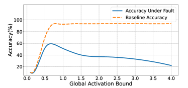
Figure 1: Accuracy of the VGG16 network on CIFAR-10 dataset under a fault rate of $10^{-5}$, with regard to different global bound values of GBReLU in the second network layer.

To better understand the source of this accuracy drop, we perform a statistical study on all neurons’ output values in the second layer of the VGG16 network. Figure 2 shows the distribution of the maximum output values for all neurons in the layer. We observe that the neurons across the layer have different maximum values; a similar trend is observed for other layers and other networks. However, the GBReLU approach [16, 17, 18] chooses a fixed upper bound value for all neurons in the layer, which may not remove some faulty output values (if $\lambda$ is too big) or may eliminate some non-faulty output values (if $\lambda$ is too small). This motivates us to explore the fine-grained bounded activation function where we can set a bound for the activation function for each neuron in the network.

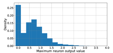
Figure 2: Distribution of the maximum output values of all neurons in VGG16’s second layer on the CIFAR-10 dataset.

IV FitReLU: Trainable Fine-Grained Bounded ReLU Activation Function

In light of our findings in Section III-C, instead of defining a bounded activation function globally, we propose to define a fine-grained bounded activation function for each neuron.

IV-A Neuron-Wise Bounded Activation Function

Neuron-wise activation function acts as a vector of activation functions in each hidden-layer, where every neuron has its own activation function, as opposed to a single global activation function shared by all neurons. In this paper, we introduce a parametric neuron-wise bounded ReLU (FitReLU-Naive) as:

$$\xi_{FitReLU-Naive}(x)=\begin{cases}0&\text{if $x>\lambda_{i}$}\\ x&\text{if $0<x\leq\lambda_{i}$}~{}~{}~{}~{}\forall{i\in\{1,...,N\}}\\ 0&\text{$x\leq 0$}\end{cases}$$ (5)

where $N$ denotes the number of neurons in the network and $\lambda_{i}$ denotes the bound value for neuron $i$. It indicates that values bigger than $\lambda_{i}$ are probably faulty for neuron $i$ and need to be controlled by its activation function.

IV-B Issue with FitReLU-Naive

To deploy the proposed FitReLU-Naive in a DNN model, we need to adjust $N$ parameters, i.e., $\lambda_{1}$ to $\lambda_{N}$, so as to improve the resilience of the model. To find the best values of $\lambda_{1}$ to $\lambda_{N}$, we will introduce a post-training phase in Section V to fine tune these values, in order to minimize the loss function and maximize the resilience. Most learning algorithms are based on the backward propagation of the error gradients. However, the derivative of the FitReLU-Naive activation function at point $x=\alpha$ cannot be computed, since it has different terms in each segment as presented in Equation 5. Therefore, it is nontrivial to learn the FitReLU-Naive activation functions (i.e., $\lambda_{1}$ to $\lambda_{N}$) via the post-training process.

IV-C Trainable FitReLU

To solve the above problem in Section IV-B, we introduce a new activation function (called FitReLU) that can be trained during the learning process [27] and has a behavior similar to FitReLU-Naive. Inspired by the sigmoid mathematical function [14], we reformulate FitReLU into a trainable one as:

$$\xi_{FitReLU}(x)=max(0,\ x-\frac{x}{1+e^{k(x-\lambda_{i})}})~{}~{}~{}\forall{i\in\{1,...,N\}}$$ (6)

where $N$ and $\lambda_{i}$ are the same as those in Equation 5, and $k$ is a coefficient to control the decent slope of the function and is empirically computed. The illustrations of both FitReLU-Naive and trainable FitReLU, as well as the original ReLU and GBReLU are presented in Figure 3.

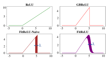
Figure 3: Representation of original ReLU [26], GBReLU (globally bounded ReLU) [18], naive FitReLU and trainable FitReLU activation functions.

V FitAct: The Proposed Resilient DNN Framework

To avoid retraining the DNN model from scratch and complicating the DNN training process, we divide our workflow (called FitAct) of building an error resilient DNN with the proposed FitReLU activation function into two separate stages. As shown in Figure 4, in the first stage, FitAct trains a DNN model with the original ReLU activation function using the conventional training process. Its goal is to learn the weight and bias parameters ($\bm{w}^{1}$ to $\bm{w}^{D}$, $\bm{b}^{1}$ to $\bm{b}^{D}$) to improve the model accuracy, without the consideration of error resilience. In the second stage, FitAct first replaces the ReLU activation function in the trained DNN model with our proposed FitReLU variants. Then it post-trains the modified DNN model to tune the fine-grained bound values ($\lambda_{1}$ to $\lambda_{N}$) of FitReLU functions to improve the model resilience against faults.

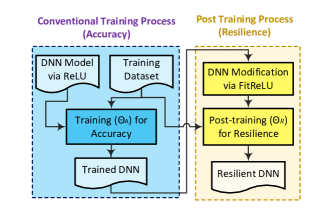
Figure 4: FitAct: our two-stage workflow to enhance the resilience of DNNs by post-training FitReLU activation functions.

Formally, the final error resilient DNN model can be represented using two separable groups of learning parameters as:

$$\bm{u}_{\Theta_{A},\Theta_{R}}(\bm{z})=(\mathscr{L}_{D}\circ\xi_{D-1}(\cdot)\circ\mathscr{L}_{D-1}\circ\xi_{D-2}(\cdot)\circ\dots\xi_{1}(\cdot)\circ\mathscr{L}_{1})(\bm{z})$$ (7)

where the set of trainable parameters $\Theta_{A}$ consists of ${\bm{w}^{k},\bm{b}^{k}}:$ ${k=1,...,D}$, which indicate the accuracy goal, and $\Theta_{R}$ denotes the post-trainable parameters, i.e., ${\lambda_{i}}:{i=1,...,N}$, which indicate the resilience goal.

Conventional Training for Accuracy: A typical learning algorithm for the training stage updates $\Theta_{A}$ through gradient computations, and calculates the errors on training dataset $\mathbb{D}$ via an accuracy loss function $\mathcal{L}(\mathbb{D};\Theta_{A})$. We denote the accuracy of the trained network as $\mathcal{A}(\Theta_{A})$.

DNN Architecture Modification: We modify the trained DNN model by replacing the original ReLU function for each neuron with our FitReLU variants, and initialize the bound parameters $\Theta_{R}$ for each neuron to their maximum values over the training dataset $\mathbb{D}$. Note that by applying this modification, the accuracy of the obtained model, $\mathcal{A}(\Theta_{A},\Theta_{R})$, would be changed.

Post-Training for Resilience Enhancement: To enhance the error resilience of the modified DNN architecture, we perform a post-training phase detailed in the following subsections.

V-A Resilience Enhancement as an Optimization Problem

The main goals of our post-training phase could be expressed as: 1) maximizing the resilience of the model, and 2) maintaining the accuracy of the model. Using goal 1 as the objective and goal 2 as the constraint, we can formulate the model resilience enhancement as the following optimization problem:

$$\begin{split}&max_{~{}\bm{{\Theta_{R}}}}(\mathcal{R}(\Theta_{A},\Theta_{R}))\\ &s.t.\quad\quad\mathcal{A}(\Theta_{A})-\mathcal{A}(\Theta_{A},\Theta_{R})<\delta\end{split}$$ (8)

where $\mathcal{R}(\Theta_{A},\Theta_{R})$ is the resilience of the model, which represents the accuracy of the modified network under faults. $\mathcal{A}(\Theta_{A},\Theta_{R})$ is the accuracy of the modified network without faults. And the threshold $\delta$ can be adjusted based on how much accuracy loss we are willing to accept for resilience boosting.

As discussed in Section III-C, having lower values of $\Theta_{R}$ could increase the chance of fault removing and thus increase the resilience. However, when the values of $\Theta_{R}$ become lower than a certain level, the accuracy loss could also increase. Therefore, we can maximize the resilience by minimizing $\Theta_{R}$ values until the accuracy loss is not acceptable. The optimization problem in Equation 8 can be reformulated as:

$$\begin{split}min({\Theta_{R}})\quad\quad s.t.\ \ \mathcal{A}(\Theta_{A})-\mathcal{A}(\Theta_{A},\Theta_{R})<\delta\end{split}$$ (9)

V-B Post-Training Algorithm

In order to minimize $\Theta_{R}$ while maintaining the accuracy (i.e., Equation 9), we introduce a post-training algorithm with a new loss function $\mathcal{L}(\mathbb{D};\Theta_{A},\Theta_{R}$). It is the same as that in the conventional training step except that it has an extra regularization restriction over the $\Theta_{R}$ parameters to penalize the increasing upper bounds. That is:

$$\mathcal{L}(\mathbb{D};\Theta_{A},\Theta_{R})=\mathcal{L}(\mathbb{D};\Theta_{A})+\frac{\zeta}{N}\sum_{i=1}^{N}\lambda_{i}^{2}$$ (10)

where $\zeta$ is a hyper parameter. Note that only bound values $\Theta_{R}$ would be adjusted and none of $\Theta_{A}$ will be changed in this step.

The solution to this problem can be approximated using an iterative gradient descent algorithm. In this work, we use the ADAM optimizer [28] to solve it, which is a widely used variant of the stochastic gradient descent algorithm.

VI Experimental Results

VI-A Experimental Setup

VI-A1 DNN Model and Dataset

We test FitAct on three widely used DNN models: AlexNet, VGG16 and ResNet50. We use 32-bit fixed-point representation (1 sign bit, 15 integeral bits and 16 fractional bits) rather than floating-point for model parameters, since it is more energy efficient. These models are trained on two different datasets: CIFAR-10 and CIFAR-100. All experiments are performed on an Intel Core i7@3.2 GHz processor with 32 GB memory and an NVIDIA TITAN V GPU.

To validate the efficacy of our approach, we compute the top-1 classification accuracy. The baseline (top-1) accuracy values without fault for CIFAR-10 dataset are 95.03%, 93.57% and 87.08%, for ResNet50, VGG16 and AlexNet models, respectively. The baseline accuracy values of CIFAR-100 dataset are 78.43%, 73.67% and 87.08% for the three models, respectively.

VI-A2 Fault Simulation

In this paper, we consider memory faults to analyze the error resilience of DNNs, where the model parameters may be affected under the injection of random bit-flips in the memory blocks that store these parameters. The weights and biases of different layers, as well as parameters of activation functions, are considered as the fault space. To simulate random fault injections, we develop a fault injection tool based on the PyTorch framework. We assume that the fault space would be distributed uniformly over random locations in the target units and throughout the inference period, which is in line with prior studies [29, 18, 16]. We perform fault injections on different fault rates ranging from $10^{-7}$ to $3\times 10^{-5}$.

VI-B Resilience Results

To demonstrate the efficacy of FitAct, we compare the model resilience under different fault rates, between our FitAct, state-of-the-art studies Clip-Act [18] and Ranger [16] that use a layer-wise globally bounded ReLU activation function to improve model resilience, as well as unprotected DNNs.

Figure 5 compares the model accuracy distribution between different approaches under different fault rates, using the VGG16 network on CIFAR-10 dataset as a case study. The accuracy of the unprotected DNN model has a huge drop to around 10% under fault injection, which clearly calls for resilience enhancement. In general, as the fault rate increases, the accuracy of the three protected DNNs decreases, because the protection becomes less effective and faults are more likely to be injected in critical bits, having a more substantial impact on the output classification. As shown in Figure 5, FitAct can keep the accuracy within an acceptable range even at a high fault rate of $10^{-5}$, whereas Clip-Act [18] and Ranger [16] experience a significant accuracy drop at fault rates higher than $10^{-6}$ and $10^{-7}$, respectively.

Figure 6 compares the average accuracy between FitAct, Clip-Act [18], Ranger [16] and unprotected model under different fault rates, for various DNN architectures and datasets. First, all three protection methods boost the accuracy under fault compared to the unprotected one, and FitAct achieves the best accuracy (i.e., resilience) among all. Second, compared to Clip-Act [18], when the fault rate becomes $3\times 10^{-6}$ or higher, FitAct achieves a significantly higher accuracy. For example, at the fault rate of $3\times 10^{-6}$, FitAct can still achieve a high accuracy of 84.81% and 90.28% for ResNet50 and VGG16 models on CIFAR-10 dataset, while Clip-Act can only achieve an accuracy of 52.47% and 61.63%. Third, Ranger [16] performs much worse than Clip-Act [18] and FitAct, even at a low fault rate of $10^{-7}$. At a higher fault rate than $10^{-7}$, Ranger is no longer effective in the protection against faults. This is because Ranger truncates an output faulty value to a big positive bound, which still propagates in the network.

Figure 5: Model accuracy distribution for FitAct, Clip-Act [18], Ranger [16] and unprotected DNN, using the VGG16 network on CIFAR-10 dataset, under different fault rates.

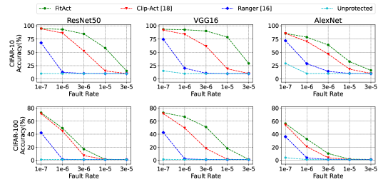
Figure 6: Average model accuracy for FitAct, Clip-Act [18], Ranger [16] and unprotected DNN models, including ResNet50, VGG16, and AlexNet models on CIFAR-10 and CAFIR-100 datasets, under different fault rates.

VI-C Time and Memory Space Overhead

VI-C1 Training Step

Since FitAct separates the conventional training for accuracy and post-training for resilience, it can maintain a small computational overhead. For example, the whole process of post-training for ResNet50, VGG16 and AlexNet models on CIFAR-10 dataset take about 21, 4 and 1 minutes, respectively. Considering the long runtime for conventional training of these models (340, 60, and 17 minutes), FitAct only adds around 5.9% to 6.7% extra runtime overhead.

TABLE I: Runtime and memory space overheads (O/H) when deploying resilient DNN with FitAct in the inference stage.

		Runtime (ms)			Memory (Mb)
		ReLU	FitAct	O/H	ReLU	FitAct	O/H
CIFAR-10	ResNet50	9.820	10.869	10.68%	156.69	165.05	5.34%
	VGG16	5.324	5.600	5.18%	29.60	30.46	2.91%
	AlexNet	3.037	3.175	4.54%	23.53	23.68	0.64%
CIFAR-100	ResNet50	9.877	10.974	11.11%	156.70	165.10	5.36%
	VGG16	5.178	5.487	5.97%	29.65	30.47	2.77%
	AlexNet	3.001	3.224	7.43 %	23.53	23.69	0.68%

VI-C2 Inference Step

Compared to the original ReLU, FitReLU (Equation 6) costs more computation and needs extra memory space to store the bound values $\lambda_{1}$ to $\lambda_{N}$. Table I presents the time and memory space overheads of FitAct for various models and datasets in the inference step. Since most of the computations and memory storage happen in the convolutional and fully connected layers, the overheads introduced by FitAct is manageable. Shown in Table I, the runtime overheads are less than 12% and the memory space overheads are less than 6%.

VII Conclusion

In this paper, we have proposed FitAct, a framework to build low-overhead error-resilient DNNs by deploying fine-grained post-trainable activation functions. First, we have proposed a fine-grained, trainable, neuron-wise activation function called FitReLU to precisely bound the activation value of each neuron, so as to prevent the fault propagation in the network. Second, we have developed a lightweight post-training phase to learn all these activation functions with precise bound values, which is decoupled from the conventional training for model accuracy. Finally, we have conducted a wide range of experiments using fault simulation and confirmed the effectiveness and advantages of our FitAct framework in enhancing the error resilience for widely used DNN models.

References

- [1] Miotto et al., “Deep learning for healthcare: review, opportunities and challenges,” Briefings in bioinformatics, vol. 19, no. 6, pp. 1236–1246, 2018.
- [2] Grigorescuet al., “A survey of deep learning techniques for autonomous driving,” Journal of Field Robotics, vol. 37, no. 3, pp. 362–386, 2020.
- [3] Shafique et al., “Robust machine learning systems: Challenges, current trends, perspectives, and the road ahead,” IEEE Design & Test, vol. 37, no. 2, pp. 30–57, 2020.
- [4] S. Mittal, “A survey on modeling and improving reliability of dnn algorithms and accelerators,” JSA, vol. 104, p. 101689, 2020.
- [5] Mahmoud et al., “Hardnn: Feature map vulnerability evaluation in cnns,” arXiv preprint arXiv:2002.09786, 2020.
- [6] Li et al., “Understanding error propagation in deep learning neural network (dnn) accelerators and applications,” in SC 2017, pp. 1–12.
- [7] Libano et al., “Selective hardening for neural networks in fpgas,” IEEE TNS, vol. 66, no. 1, pp. 216–222, 2018.
- [8] Sabih et al., “Fault-tolerant low-precision dnns using explainable ai,” in DSN-W 2021. IEEE, pp. 166–174.
- [9] Hari et al., “Making convolutions resilient via algorithm-based error detection techniques,” IEEE TDSC 2021.
- [10] Dos et al., “Analyzing and increasing the reliability of convolutional neural networks on gpus,” IEEE TR, vol. 68, no. 2, pp. 663–677, 2018.
- [11] Kosaian et al., “Arithmetic-intensity-guided fault tolerance for neural network inference on gpus,” arXiv preprint arXiv:2104.09455, 2021.
- [12] Dias et al., “Ftset-a software tool for fault tolerance evaluation and improvement,” Neural Computing and Applications, vol. 19, no. 5, pp. 701–712, 2010.
- [13] Schorn et al., “An efficient bit-flip resilience optimization method for deep neural networks,” in DATE 2019. IEEE, pp. 1507–1512.
- [14] Nwankpa et al., “Activation functions: Comparison of trends in practice and research for deep learning,” arXiv preprint arXiv:1811.03378, 2018.
- [15] Liew et al., “Bounded activation functions for enhanced training stability of deep neural networks on visual pattern recognition problems,” Neurocomputing, vol. 216, pp. 718–734, 2016.
- [16] Chen et al., “A low-cost fault corrector for deep neural networks through range restriction,” in DSN 2021. IEEE, pp. 1–13.
- [17] Hong et al., “Terminal brain damage: Exposing the graceless degradation in deep neural networks under hardware fault attacks,” in USENIX Security 2019, pp. 497–514.
- [18] Hoang et al., “Ft-clipact: Resilience analysis of deep neural networks and improving their fault tolerance using clipped activation,” in DATE 2020. IEEE, pp. 1241–1246.
- [19] Ali et al., “Erdnn: Error-resilient deep neural networks with a new error correction layer and piece-wise rectified linear unit,” IEEE Access, vol. 8, pp. 158 702–158 711, 2020.
- [20] Motors, Tesla, “Full self-driving hardware on all cars,” 2019. [Online]. Available: https://www.tesla.com/autopilot
- [21] Kim et al., “Matic: Learning around errors for efficient low-voltage neural network accelerators,” in DATE 2008. IEEE, pp. 1–6.
- [22] Jia et al., “Calibrating process variation at system level with in-situ low-precision transfer learning for analog neural network processors,” in DAC 2018, pp. 1–6.
- [23] Mhamdi et al., “When neurons fail,” arXiv preprint arXiv:1706.08884, 2017.
- [24] Zahid et al., “Fat: Training neural networks for reliable inference under hardware faults,” in ITC 2020. IEEE, pp. 1–10.
- [25] Krizhevsky et al., “Imagenet classification with deep convolutional neural networks,” NIPS 2012, vol. 25, pp. 1097–1105.
- [26] Arora et al., “Understanding deep neural networks with rectified linear units,” arXiv preprint arXiv:1611.01491, 2016.
- [27] Apicella et al., “A survey on modern trainable activation functions,” Neural Networks, 2021.
- [28] Kingma et al., “Adam: A method for stochastic optimization,” arXiv preprint arXiv:1412.6980, 2014.
- [29] Reagen et al., “Ares: A framework for quantifying the resilience of deep neural networks,” in DAC 2018. IEEE, pp. 1–6.