Family Floer superpotential’s critical values are eigenvalues of quantum product by $c_{1}$

Abstract

Abstract: In the setting of the non-archimedean SYZ mirror construction in [Yua20], we prove the folklore conjecture that the critical values of the mirror superpotential are the eigenvalues of the quantum multiplication by the first Chern class. Our result relies on a weak unobstructed assumption, but it is usually ensured in practice by Solomon’s results [Sol20] on anti-symmetric Lagrangians. Finally, we also present some explicit examples based on the very recent progress [Yua22].

1 Introduction

The mirror symmetry phenomenon does not merely focus on the Calabi-Yau setting. Assume that a compact symplectic manifold $(X,\omega)$ is Fano (or more generally that $-K_{X}$ is nef). The mirror of $X$ is expected to be a Landau-Ginzburg model $(X^{\vee},W^{\vee})$ consisting of a space $X^{\vee}$ equipped with a global function $W^{\vee}$ called the superpotential. In the context of the homological mirror symmetry [Kon95], a celebrated folklore conjecture states that: (known to Kontsevich and Seidel, compare also [She16, §2.9])

Conjecture 1.1.

The critical values of the mirror Landau-Ginzburg (LG) superpotential $W^{\vee}$ are the eigenvalues of the quantum multiplication by the first Chern class of $X$.

The conjecture is first proved by Auroux [Aur07] in the Fano toric case, concerning the Landau-Ginzburg mirror associated to a toric Lagrangian fibration in $X$ [CO06, FOOO10a].

Theorem 1.2.

Conjecture 1.1 holds for the family Floer mirror Landau-Ginzburg superpotential.

In brief, we aim to prove the conjecture with nontrivial Maslov-0 quantum correction, and actually we don’t need to be limited to the family Floer scope (see §1.2 for the precise statement). It looks like a “small” step to include Maslov-0 disks, but it is indeed difficult and requires many new ideas (§1.3). We also find new examples recently in [Yua22] to justify and amplify the value of this paper (§1.1).

The symplectic-geometric ideas we use are not original, but it is not our main point at all. Instead, a major point in this paper is to demonstrate that the classical ideas fit perfectly into the framework of the family Floer mirror construction in [Yua20]. For example, a key new ingredient for our proof is a preliminary version of “Fukaya category with affinoid coefficients” (i.e. the self Floer cohomology for $\mathscr{UD}$ in §3). Roughly, the coefficient we use is not $\mathbb{C}$, not the Novikov field $\Lambda$, but an affinoid algebra over $\Lambda$. The merit is that we can ignore all the affects of Maslov-0 disk obstruction up to affinoid algebra isomorphism on the coefficients using the ideas in the author’s thesis [Yua20]. We expect the affinoid coefficients should be important to develop Abouzaid’s family Floer functor [Abo17, Abo21] with Maslov-0 corrections. A work in progress is [Yua]. For the above speculative version of Fukaya category, one might study many topics like splitting generations [AFO⁺] and Bridgeland stability conditions (cf. [Smi17] [Kon]) in some similar ways in future studies. We also expect that it is related to the non-archimedean geometry, like the coherent analytic sheaves, on the family Floer mirror space, potentially being the analytification of an algebraic variety over the Novikov field. But unfortunately, the precondition of all the story is to allow the Maslov-0 disks in the course. Otherwise, we cannot even realize a simple algebraic variety like $Y=\{x_{0}x_{1}=1+y\}$ as a family Floer mirror space and thus miss the new examples of Conjecture 1.1 in §1.1 and [Yua22].

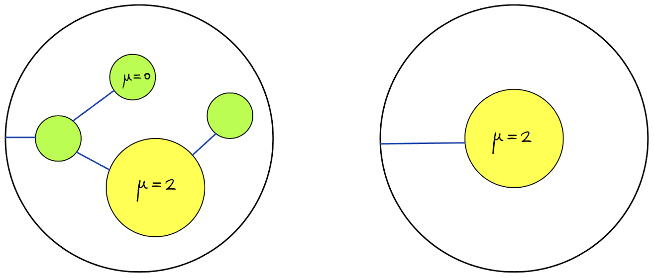
Figure 1: A piece of contribution to the LG superpotential with / without the Maslov-0 quantum correction. When we perturb $J$, all the Maslov-0 disks (green) in the Feynman-diagrams of the minimal model $A_{\infty}$ algebras are continually created and annihilated for the wall-crossing. This is more like a sort of “quantum fluctuation”. This is why the LG superpotential is only well-defined up to affinoid algebra isomorphism.

(1) What is the difficulty of allowing Maslov-0 corrections?

First and foremost, the family Floer mirror superpotential is only well-defined up to affinoid algebra isomorphisms, or equivalently, up to family Floer analytic transition maps [Yua20]. This is because the Maslov-0 quantum correction give rise to certain mirror non-archimedean analytic topology. Note that the idea of uniting Maurer-Cartan sets, adopted by Fukaya and Tu [Fuk09, Fuk11, Tu14], cannot achieve the family Floer mirror non-archimedean analytic structure. We must go beyond their Maurer-Cartan picture; otherwise, although Fukaya and Tu did tell the correct local analytic charts, the local-to-global gluing was only set-theoretic. In fact, we never think of bounding cochains but work with formal power series in the corresponding affinoid algebra directly [Yua20]. One of many crucial flaws in the previous work concerns the lack of studies of the divisor axiom for $A_{\infty}$ structures. The ud-homotopy theory developed in [Yua20] is indispensable for the mirror analytic gluing. Remarkably, the ud-homotopy theory plays the key role for the folklore conjecture once again (cf. §1.3).

Putting another way, we must work with the minimal model $A_{\infty}$ algebras, while paying attention to the wall-crossing phenomenon simultaneously (Figure 1). Without minimal model $A_{\infty}$ algebras, the superpotential would be only $\Omega^{0}(L)$-valued and was not well-defined. This issue was not so fatal if the Maslov indices $>0$, but it is indeed fatal if we allow Maslov-0 correction. As another evidence, a minimal model $A_{\infty}$ algebra is intuitively like counting holomorphic pearly-trees (cf. [FOOO09]) which are also used in Sheridan’s proof of HMS of Calabi-Yau projective hypersurfaces [She15, §6.2]. The conventional ideas of the folklore conjecture cannot work or need to be improved for holomorphic pearly-trees or minimal model $A_{\infty}$ algebras, if nontrivial Maslov-0 disks exist (Figure 1). A daunting trouble is to handle the minimal model $A_{\infty}$ algebra’s Hochschild cohomology (see §1.3).

(2) Why does the family Floer method give a convincing approach to construct the mirror?

The answer in short is simply that we can prove the Conjecture 1.1 supported by examples below.

Gross and Siebert proposed a method of mirror construction in the algebro-geometric framework [GS11] based on the SYZ proposal [SYZ96]. By its philosophy, Gross-Hacking-Keel [GHK15] give a synthetic construction of the mirror family for local Calabi-Yau surfaces. The algebro-geometric mirror symmetry approach turns out to be successful in many aspects, such as [HK20, GHK13, GHKK18]. But, in our biased opinion, the folklore Conjecture 1.1 inevitably relies on Floer-theoretic or symplectic-geometric ideas in the end. The family Floer mirror construction [Yua20] can naturally include the Landau-Ginzburg superpotential. In reality, such a Floer-theoretic mirror construction succeeded in rigorizing the T-duality of smooth Lagrangian torus fibration with full quantum correction considered, and leads to a mathematical precise statement of SYZ conjecture with singularities in [Yua22].

1.1 New examples

Due to the very recent [Yua22], we can explicitly write down some new examples (see §1.1) for the folklore conjecture as follows. For simplicity, we only consider a simple case of dimension 2. Let

$$X=\mathbb{C}^{2}\setminus\{z_{1}z_{2}=1\}$$

and take the standard symplectic form on $\mathbb{C}^{2}$. Consider the special Lagrangian fibration $\pi:X\to\mathbb{R}^{2}$ defined by (cf. [Gro01, Aur07])

(1) $$\pi(z_{1},z_{2})=(\tfrac{|z_{1}|^{2}-|z_{2}|^{2}}{2},\log|z_{1}z_{2}-1|)$$

There is a piecewise smooth function $\psi:\mathbb{R}^{2}\to\mathbb{R}_{+}$, represented by the symplectic areas of a family of disks, such that $(\frac{1}{2}(|z_{1}|^{2}-|z_{2}|^{2}),\psi)$ locally forms the action coordinates. It is basically standard and intuitively illustrated in Figure 2. See also [Yua22].

Figure 2: The symplectic areas of disks for the function $\psi$

The SYZ mirror of $X$ is the algebraic variety:

$$Y=\{(x_{0},x_{1},y)\in\Lambda^{2}\times\Lambda^{*}\mid x_{0}x_{1}=1+y\}$$

over the Novikov field

$$\textstyle\Lambda=\mathbb{C}((T^{\mathbb{R}}))=\Big{\{}\sum_{i=0}^{\infty}a_{i}T^{\lambda_{i}}\mid a_{i}\in\mathbb{C},\lambda_{i}\in\mathbb{R},\lambda_{i}\to\infty\Big{\}}$$

It has a natural non-archimedean valuation $\mathsf{v}:\Lambda\to\mathbb{R}\cup\{\infty\}$ that also induces a norm $|x|=e^{-\mathsf{v}(x)}$. Consider a Zariski-dense analytic open domain

$$\mathscr{Y}=\{|x_{1}|<1\}$$

in the analytification $Y^{\mathrm{an}}$ of $Y$. Alternatively, we think of $\mathscr{Y}$ as the family Floer mirror analytic space that can embed into $Y^{\mathrm{an}}$. For clarity, from now on, we will not distinguish $Y$ and $Y^{\mathrm{an}}$.

Remark 1.3

We do not want to elaborate on the Berkovich geometry behind and only give short remark. Just like the analytification of an algebraic variety over $\mathbb{C}$, we can speak of the Zariski topology and the (non-archimedean) analytic topology simultaneously on an algebraic variety over $\Lambda$, like the above $Y$ (e.g. [Tem15]). Indeed, there is a non-archimedean GAGA principle. Thinking in the set-theoretic level, $Y^{\mathrm{an}}$ consists of the closed points of the variety $Y$ together with certain ‘generic points’ in the Berkovich sense (e.g. [Bak08]). It is similar to, but in a different flavor, how we add generic points of prime ideals into a variety to make a scheme. For simplicity, one may also content with the rigid analytification $T^{\mathrm{rig},\mathrm{an}}$ which set-theoretically only keeps the closed points of $Y$. In reality, there is a one-one correspondence between rigid analytic spaces and good Berkovich analytic spaces (e.g. [Ber93]).

A remarkable discovery in [Yua22] is that there is an analytic map $f:\mathscr{Y}\to\mathbb{R}^{2}$ so that the smooth locus, the singular locus, and the induced integral affine structure of $f$ all precisely agree with those of $\pi$. It is very similar to and is indeed inspired by Kontsevich-Soibelman’s singular model [KS06, §8], but we must have extra data in order to make connections with the A-side. One of the explicit representations of $f$ involves a topological embedding

$$j:\mathbb{R}^{2}\to\mathbb{R}^{3},\quad j(q_{1},q_{2})=\begin{pmatrix}\min\{-\psi(q_{1},q_{2}),-\psi(q_{1},0)\}+\min\{0,q_{1}\}\\ \min\{\psi(q_{1},q_{2}),\psi(q_{1},0)\}\\ q_{1}\end{pmatrix}$$

and an analytic map

$$F:\mathscr{Y}\to\mathbb{R}^{3},\quad F(x_{0},x_{1},y)=\begin{pmatrix}\min\Big{\{}\mathsf{v}(x_{0}),-\psi(\mathsf{v}(y),0)+\min\{0,\mathsf{v}(y)\}\Big{\}}\\ \min\{\mathsf{v}(x_{1}),\psi(\mathsf{v}(y),0)\}\\ \mathsf{v}(y)\end{pmatrix}$$

where the $\mathsf{v}$ is the non-archimedean valuation and the $\psi$ comes from the A-side (1).

Somewhat surprisingly, with some efforts, it follows directly from the above formulas that

$$j(\mathbb{R}^{2})=F(\mathscr{Y})$$

Thus, we are able to define

(2) $$f=j^{-1}\circ F:\mathscr{Y}\to\mathbb{R}^{2}$$

By the mere formula above, one can directly check the aforementioned affine geometry coincidence in the base $\mathbb{R}^{2}$ between $f$ and $\pi$, for which there is no need for any Floer theory. But, there is a more refined T-duality between $f$ and $\pi$ concerning the family Floer mirror construction as shown in [Yua22].

By the general theories in [Yua20], the various (partial) compactification $\overline{X}$ of $X$ gives rise to the various mirror Landau-Ginzburg superpotential $W^{\vee}$ on the same algebraic variety $Y$. One may deform the symplectic form $\omega$ to induce various $W^{\vee}$ on the same variety $Y=\{x_{0}x_{1}=1+y\}$. For clarity, we only consider two special examples of compactification spaces $\overline{X}=\mathbb{CP}^{2}$ and $\mathbb{CP}^{1}\times\mathbb{CP}^{1}$ below to illustrate our result:

Ambient space	$\overline{X}=\mathbb{CP}^{2}$	$\overline{X}=\mathbb{CP}^{1}\times\mathbb{CP}^{1}$
LG superpotential	$W^{\vee}=x_{1}+\frac{T^{E(\mathcal{H})}x^{2}_{0}}{y}$	$W^{\vee}=x_{1}+\frac{T^{E(\mathcal{H}_{1})}x_{0}}{y}+T^{E(\mathcal{H}_{2})}x_{0}$
Critical points	$\begin{cases}x_{0}=T^{\frac{-E(\mathcal{H})}{3}}e^{\frac{-2\pi is}{3}}\\ x_{1}=2T^{\frac{E(\mathcal{H})}{3}}e^{\frac{2\pi is}{3}}\ \ s=0,1,2\\ y=1\end{cases}$	$\begin{cases}x_{0}=\pm T^{\frac{-E(\mathcal{H}_{2})}{2}}\\ x_{1}=\pm T^{\frac{E(\mathcal{H}_{1})}{2}}\pm T^{\frac{E(\mathcal{H}_{2})}{2}}\\ y=\pm T^{\frac{E(\mathcal{H}_{1})-E(\mathcal{H}_{2})}{2}}\end{cases}$
Critical values	$3T^{\frac{E(\mathcal{H})}{3}}e^{\frac{2\pi is}{3}}$ ($s=0,1,2$)	$\pm 2T^{\frac{E(\mathcal{H}_{1})}{2}}\pm 2T^{\frac{E(\mathcal{H}_{2})}{2}}$

Just by routine computations, we can find the above critical points and critical values.

The Landau-Ginzburg superpotentials seem to be new. Actually, if we eliminate $x_{1}$ or $x_{0}$ via the definition equation $x_{0}x_{1}=1+y$ of $Y$, we more or less go back to the previous Clifford or Chekanov superpotentials but in a non-archimedean setting (cf. [PT20]). In other words, ours should be of a more global nature. This phenomenon is more clear in higher dimensions (cf. [Yua22, Yua21]).

Even for a fixed ambient space $\overline{X}$, we may obtain infinitely many LG superpotentials $W^{\vee}$ parameterized by the various symplectic forms $\omega$. But, we can still show that Conjecture 1.1 holds for all of them. Our computations of the critical values in the two cases in the table agree with the $c_{1}$-eigenvalues as in Conjecture 1.1 (cf. [FOOO10a, Example 5.2 & 5.6]).

Admittedly, the value of our result may rely on future examples we would find. But, the critical points are quite sensitive to the choices and are not guaranteed to avoid the walls of Maslov-0 disks in general. For one thing, there can be infinitely many walls [Aur15, §5]. For another, the walls may be dispersed in an open subset in the base, say, for the blowup of $\mathbb{C}^{n}$ along a hypersurface [Aur08, Example 3.3.2] (c.f. also [AAK16]). Moreover, in our specific situation, we cannot find the walls from the formula of $f$ in (2), although the $f$ truly comes from the wall-crossing gluing. Indeed, there is no any discontinuity of the wall-crossing phenomenon as long as we use the non-archimedean topology. The walls (relying on $J$) are often not detectable from the mirror non-archimedean analytic structure (not relying on $J$ up to isomorphism). Therefore, in general, we need to include Maslov-0 disks in the story.

1.2 Main result

Let $(X,\omega)$ be a symplectic manifold which is closed or convex at infinity. Let $\dim_{\mathbb{R}}X=2n$. Let $L$ be an oriented, spin, and compact Lagrangian submanifold satisfying the semipositive condition that prohibits any nontrivial negative Maslov index holomorphic disk. In practice, a graded or special Lagrangian submanifold is always semipositive by [Aur07, Lemma 3.1]. Given an $\omega$-tame almost complex structure $J$, we can associate to $L$ a superpotential function

(3) $$W_{L}:=W_{L}^{J}=\sum_{\beta\in\pi_{2}(X,L),\mu(\beta)=2}T^{E(\beta)}Y^{\partial\beta}\mathfrak{m}_{0,\beta}$$

where we use the minimal model $A_{\infty}$ algebra

$$\mathfrak{m}=(\mathfrak{m}_{k,\beta})_{k\in\mathbb{N},\beta\in\pi_{2}(X,L)}$$

of the cochain-level $A_{\infty}$ algebra associated to $L$. Here we work over the Novikov field $\Lambda=\mathbb{C}((T^{\mathbb{R}}))$, $Y$ is a formal symbol, so $W_{L}\in\Lambda[[\pi_{1}(L)]]$. The reverse isoperimetric inequality [GS14] ensures that $W_{L}$ converges on an analytic open neighborhood of $H^{1}(L;U_{\Lambda})$ in $H^{1}(L;\Lambda^{*})$.

Although the summation in (3) runs only over Maslov-2 topological disks $\beta$, it actually can involve all the possible Maslov-0 obstruction in the same time. This is simply the natural of minimal model $A_{\infty}$ algebras, and the idea is illustrated in Figure 1. In general, allowing the Maslov-0 disks, the superpotential function $W_{L}^{J}$ is not well-defined and rely on the various choices like $J$. But, as in [Yua20] (or see Lemma 2.6), we can show that the $W_{L}$ is well-defined up to affinoid algebra isomorphism, and we can also show that the critical points and critical values are preserved.

Assumption 1.4.

The formal power series $Q_{L}^{J}:=\sum_{\mu(\beta)=0}T^{E(\beta)}Y^{\partial\beta}\mathfrak{m}_{0,\beta}$ vanishes identically.

We often denote by ${\mathfrak{a}}$ the ideal generated by the components of $Q_{L}^{J}$. Then, the above means ${\mathfrak{a}}$ vanishes. Be cautious that the above assumption never says the counts of Maslov-0 disks vanish. They still contribute to both the minimal model $A_{\infty}$ algebras and the wall-crossing phenomenon. Moreover, it is not a restrictive assumption. Thanks to the work of Solomon [Sol20], a very useful sufficient condition of the above Assumption 1.4, which we often adopt in practice, is given as follows:

Assumption 1.5.

There is an anti-symplectic involution $\varphi$ that preserves $L$.

Indeed, such a $\varphi$ gives a pairing on $\pi_{2}(X,L)$ via $\beta\xleftrightarrow{}-\varphi_{*}\beta$. Then, the Maslov-0 obstruction terms $\mathfrak{m}_{0,\beta}$ in $Q_{L}^{J}$ are then canceled pairwise. In practice, such an involution $\varphi$ is often not hard to find. For example, any Lagrangian fiber of $\pi$ in (1) is preserved by the complex conjugate $z_{i}\mapsto\bar{z}_{i}$ (see also [CBMS10]). Note that the vanishing of $Q_{L}^{J}$ does not rely on $J$ due to [Yua20]. Beware that we have not discuss the family Floer setting or the SYZ setting at this moment. Note also that we do not require $L$ is a torus here.

Now, we state the main result.

Theorem A (Theorem 5.5).

Under Assumption 1.4, if the cohomology ring $H^{*}(L)$ is generated by $H^{1}(L;\mathbb{Z})$, then any critical value of $W_{L}$ is an eigenvalue of the quantum product by $c_{1}$. Moreover, the same result still holds if we use different choices.

It is conceivable that if the above $L$ lives in a family of Lagrangian submanifolds $\{L_{q}\}$, then one may extend the domain of $W_{L}$ to a larger open analytic space. Up to the Fukaya’s trick, this amounts to study how $W_{L}$ depends on the choice of $J$. Recall that $W_{L}$ is only invariant up to affinoid algebra isomorphisms. This is because of a sort of ‘quantum fluctuation’, when we think of the minimal model $A_{\infty}$ algebra together with the wall-crossing phenomenon in the meantime (see Figure 1).

1.2.1 Family Floer mirror construction setting

As a byproduct of the above Theorem A, we can verify the family Floer mirror superpotential in [Yua20] respects Conjecture 1.1. We first briefly review it. Suppose $(X,\omega)$ is a symplectic manifold which is closed or convex at infinity. Suppose there is a smooth Lagrangian torus fibration $\pi_{0}:X_{0}\to B_{0}$ in an open subset $X_{0}$ in $X$ over a half-dimensional integral affine manifold $B_{0}$. Suppose that $\pi_{0}$ is semipositive in the sense that any holomorphic disk bounding a fiber $L_{q}:=\pi_{0}^{-1}(q)$ has a non-negative Maslov index. By [Aur07], a sufficient condition is to assume $\pi_{0}$-fibers are graded or special Lagrangians. For simplicity, we also require that the $\pi_{0}$-fibers satisfy Assumption 1.4 or 1.5. Then, we state the result of SYZ duality with quantum correction considered:

Theorem 1.6 ([Yua20]).

We can naturally associate to the pair $(X,\pi_{0})$ a triple $\mathbb{X}^{\vee}:=(X_{0}^{\vee},W_{0}^{\vee},\pi_{0}^{\vee})$ consisting of a non-archimedean analytic space $X_{0}^{\vee}$ over $\Lambda$, a global analytic function $W_{0}^{\vee}$, and an affinoid torus fibration $\pi_{0}^{\vee}:X_{0}^{\vee}\to B_{0}$ such that the following properties hold:

1. The analytic structure of $X_{0}^{\vee}$ is unique up to isomorphism.

2. The integral affine structure on $B_{0}$ from $\pi_{0}^{\vee}$ coincides with the one from the fibration $\pi_{0}$.

3. The set of closed points in $X_{0}^{\vee}$ coincides with $\bigcup_{q\in B_{0}}H^{1}(L_{q};U_{\Lambda})$.

Notice that this mirror construction uses holomorphic disks in $X$ rather than just in $X_{0}$, and we should place $\pi_{0}$ inside $X$ to understand the statement. For simplicity, we often omit the subscripts $0$’s, so we often write $(X^{\vee},W^{\vee},\pi^{\vee})$, if there is no confusion. The ud-homotopy theory and the category $\mathscr{UD}$ in [Yua20] is indispensable for the non-archimedean analytic topology in Theorem 1.6. The usual homotopy theory can only achieve a gluing in the set-theoretic level. Very intuitively, the family Floer theory is ‘algebrized’ by the category $\mathscr{UD}$, and the choice issues are all controlled by the ud-homotopy relations in $\mathscr{UD}$.

Theorem B.

Conjecture 1.1 holds for the mirror Landau-Ginzburg model in Theorem 1.6. Namely, any critical value of $W^{\vee}$ must be an eigenvalue of the quantum product by the first Chern class $c_{1}$ of $X$.

Roughly, by allowing the wall-crossing invariance, we can enlarge the domain of the superpotential and so potentially cover more eigenvalues. But, we cannot conversely conclude that all the eigenvalues of $c_{1}$ are realized by a critical point of the superpotential. Note that the $\Lambda$-coefficients in $W^{\vee}$ include the data of symplectic areas and can tell which chambers the critical points are situated in. In particular, the locations of critical points depend on the symplectic form $\omega$; see §1.1.

1.3 A new operator for Hochschild cohomology and ud-homotopy theory

The obstructions in Lagrangian Floer theory cause issues for both analysis and algebra. Definitely, the analysis part is of most importance and difficulty, concerning the complicated transversality issues of moduli spaces of pseudo-holomorphic curves. This is studied and developed by [FOOO10b, FOOO10c, FOOO20] and so on. In comparison, the algebra part should be minor. But, in our biased opinion, the intricacies and subtleties of the algebra part are greatly underestimated.

The open string Floer theoretic invariants often depend on choices. Thus, we often must talk about certain equivalence relations, depending on which the information we miss can vary. For example, in the literature like [FOOO10b], we usually talk about $A_{\infty}$ algebras up to homotopy equivalence. It is fine in most cases, but it may be too coarse in case we need more information. In reality, the homotopy equivalence relation cannot distinguish between a minimal model $A_{\infty}$ algebra and its original. This is also why the usual Maurer-Cartan picture [Fuk09, Fuk11, Tu14] cannot be enough for a local-to-global gluing for the family Floer mirror analytic structure, as explained before.

In our specific situation here for the folklore Conjecture 1.1, we must carefully distinguish between a minimal model $A_{\infty}$ algebra, denoted by $(H^{*}(L),\mathfrak{m})$, and its original, denoted by $(\Omega^{*}(L),\check{\mathfrak{m}})$. This is because the classic ideas for the folklore conjecture can only achieve connections between the quantum cohomology and the cochain-level Hochschild cohomology $HH(\Omega^{*}(L),\check{\mathfrak{m}})$. Meanwhile, the family Floer Landau-Ginzburg superpotential comes from the minimal model $A_{\infty}$ algebra $(H^{*}(L),\mathfrak{m})$.

The new challenges are enormous. For instance, the Hochschild cohomology is just not functorial, and in pure homological algebra, it is basically impossible to make any meaningful connections between the Hochschild cohomologies of a minimal model $A_{\infty}$ algebra and its original. Fortunately, in our specific geometric situation (with Assumption 1.4 or 1.5), we magically make an effective connection by the following operation (see (54))

$$\Theta:\varphi\mapsto(\mathfrak{i}^{-1}\{\varphi\})\diamond\mathfrak{i}=\sum(-1)^{*}\ \mathfrak{i}^{-1}\big{(}\mathfrak{i},\dots,\mathfrak{i},\varphi(\mathfrak{i},\dots,\mathfrak{i}),\mathfrak{i},\dots,\mathfrak{i}\big{)}$$

where $\diamond$ is the composition (see [She15]), the $\{\}$ is the celebrated brace operation (see [Get93]), and the $\mathfrak{i}^{-1}$ is the ud-homotopy inverse of the natural $A_{\infty}$ homotopy equivalence $\mathfrak{i}:\mathfrak{m}\to\check{\mathfrak{m}}$ in the course of homological perturbation. The most difficult part of the whole paper is to find the above $\Theta$. As far as we know, such $\Theta$ does not appear in any literature and seems to be exclusive for our ud-homotopy theory in [Yua20].

Now, the ud-homotopy theory shows its necessity again. Moreover, it is interesting to note that the family Floer mirror analytic gluing in [Yua20] does not exploit the full information of ud-homotopy relations, while the techniques in the present paper (e.g. the self Floer cohomology for $\mathscr{UD}$ in §3) use more information of ud-homotopy relations.

2 Preliminaries and reviews

The Floer theory usually works over the Novikov field $\Lambda=\mathbb{C}((T^{\mathbb{R}}))$. It has a valuation map $\operatorname{\mathsf{v}}:\Lambda\to\mathbb{R}\cup\{\infty\}$, sending a nonzero series $\sum a_{i}T^{\lambda_{i}}$ to the smallest $\lambda_{i}$ with $a_{i}\neq 0$ and sending the zero series to $\infty$. The Novikov ring is the valuation ring $\Lambda_{0}:=\operatorname{\mathsf{v}}^{-1}[0,\infty]$ whose maximal ideal is $\Lambda_{+}:=\operatorname{\mathsf{v}}^{-1}(0,\infty]$. The multiplicative group of units is $U_{\Lambda}:=\operatorname{\mathsf{v}}^{-1}(0)$. Note that $U_{\Lambda}=\mathbb{C}^{*}\oplus\Lambda_{+}$ and $\Lambda_{0}=\mathbb{C}\oplus\Lambda_{+}$. The standard isomorphism $\mathbb{C}^{*}\cong\mathbb{C}/2\pi i\mathbb{Z}$ naturally extends to $U_{\Lambda}\cong\Lambda_{0}/2\pi i\mathbb{Z}$. In particular, for any $y\in U_{\Lambda}$, there exists some $x\in\Lambda_{0}$ with $y=\exp(x)$.

Let $\Lambda^{*}=\Lambda\setminus\{0\}$, and we consider the tropicalization map

(4) $$\operatorname{\mathfrak{trop}}\equiv\operatorname{\mathsf{v}}^{\times n}:(\Lambda^{*})^{n}\to\mathbb{R}^{n}$$

The total space $(\Lambda^{*})^{n}$ is a rigid analytic space. Let $\Delta$ be a rational polyhedron in $\mathbb{R}^{n}$, then the preimage $\operatorname{\mathfrak{trop}}^{-1}(\Delta)$ is an affinoid subdomain. Finally, we recall an important observation in [Yua20] as follows:

Lemma 2.1.

$f\in\Lambda[[Y_{1}^{\pm},\dots,Y_{n}^{\pm}]]$ vanishes identically if and only if $f|_{U_{\Lambda}^{n}}\equiv 0$.

2.1 Gapped $A_{\infty}$ algebras and the category $\mathscr{UD}$

We review the notations and terminologies in [Yua20, §2] but we also need to introduce new things.

2.1.1 Gappedness

A label group is a triple $(\mathfrak{G},E,\mu)$ consisting of an abelian group $\mathfrak{G}$ and two group homomorphisms $E:\mathfrak{G}\to\mathbb{R}$ and $\mu:\mathfrak{G}\to 2\mathbb{Z}$. For instance, let $X$ and $L$ denote a symplectic manifold and a Lagrangian submanifold, then we may take $\mathfrak{G}=\pi_{2}(X,L)$ (or more precisely, $\mathfrak{G}$ is the image of Hurewicz map $\pi_{2}(X,L)\to H_{2}(X,L)$); the $E$ and $\mu$ are the energy and Maslov index. If $C,C^{\prime}$ are graded $\mathbb{R}$-vector spaces, then given $k\in\mathbb{N}$ and $\beta\in\mathfrak{G}$, we use the notation $\operatorname{\mathbf{CC}}_{k,\beta}(C,C^{\prime})$ to denote a copy of $\operatorname{Hom}(C^{\otimes k},C^{\prime})$ where $\beta$ is just an extra index. Consider the space

(5) $$\operatorname{\mathbf{CC}}(C,C^{\prime}):=\operatorname{\mathbf{CC}}_{\mathfrak{G}}(C,C^{\prime})\subset\prod_{k\in\mathbb{N}}\prod_{\beta\in\mathfrak{G}}\operatorname{\mathbf{CC}}_{k,\beta}(C,C^{\prime})$$

consisting of the operator systems $\mathfrak{t}=(\mathfrak{t}_{k,\beta})$ satisfying the following gappedness conditions:

• $\mathfrak{t}_{0,0}=0$;

• if $E(\beta)<0$ or $E(\beta)=0$, $\beta\neq 0$, then $\mathfrak{t}_{\beta}:=(\mathfrak{t}_{k,\beta})_{k\in\mathbb{N}}$ vanishes identically;

• for any $E_{0}>0$, there are only finitely many $\beta$ such that $\mathfrak{t}_{\beta}\neq 0$ and $E(\beta)\leq E_{0}$.

Here a collection of multilinear maps is called an operator system $\mathfrak{t}$. If it is further contained in $\operatorname{\mathbf{CC}}(C,C^{\prime})$, namely, it satisfies the above three conditions, the $\mathfrak{t}$ is called ($\mathfrak{G}$-)gapped. Unless we further specify, everything is gapped from now on. We often abbreviate it to $\operatorname{\mathbf{CC}}_{\mathfrak{G}}$ or $\operatorname{\mathbf{CC}}$.

2.1.2 Signs and degrees

Define the shifted degree $\deg^{\prime}x:=\deg x-1$ for $x\in C$. It is convenient to set

(6) $$x^{\#}=\mathrm{id}^{\#}(x)=\mathrm{id}_{\#}(x)=(-1)^{\deg x-1}x=(-1)^{\deg^{\prime}x}x$$

Given $s\in\mathbb{N}$ and a multi-linear map $\phi$, we put $\phi^{\#s}=\phi\circ\mathrm{id}^{\#s}$ where $\mathrm{id}^{\#s}$ denotes the $s$-iteration $\mathrm{id}^{\#}\circ\cdots\circ\mathrm{id}^{\#}$ of $\mathrm{id}^{\#}$. If $s=1$, we set $\phi^{\#}=\phi^{\#1}$. Let $\deg\phi$ be the usual degree as a homogeneously-graded $k$-multilinear operator among graded vector spaces. Then, the shifted degree is $\deg^{\prime}\phi=\deg\phi+k-1$. Note that $\phi^{\#}=(-1)^{\deg^{\prime}\phi}\ \mathrm{id}^{\#}\circ\phi$.

We define the composition and the Gerstenhaber product on $\operatorname{\mathbf{CC}}\equiv\operatorname{\mathbf{CC}}_{\mathfrak{G}}\subset\prod_{k,\beta}\operatorname{\mathbf{CC}}_{k,\beta}$:

(7) $$(\mathfrak{g}\diamond\mathfrak{f})_{k,\beta}=\sum_{\ell\geq 1}\sum_{k_{1}+\dots+k_{\ell}=k}\sum_{\beta_{0}+\beta_{1}+\cdots+\beta_{\ell}=\beta}\mathfrak{g}_{\ell,\beta_{0}}\circ(\mathfrak{f}_{k_{1},\beta_{1}}\otimes\cdots\otimes\mathfrak{f}_{k_{\ell},\beta_{\ell}})$$

$$(\mathfrak{g}\{\mathfrak{h}\})_{k,\beta}=\sum_{\lambda+\mu+\nu=k}\sum_{\beta^{\prime}+\beta^{\prime\prime}=\beta}\mathfrak{g}_{\lambda+\mu+1,\beta^{\prime}}\circ(\mathrm{id}_{\#\deg^{\prime}\mathfrak{h}}^{\lambda}\otimes\mathfrak{h}_{\nu,\beta^{\prime\prime}}\otimes\mathrm{id}^{\mu})$$

The gappedness ensures that they are finite sums. For instance, if $\mathfrak{f}_{0,0}$ could be non-zero, the sum in $\mathfrak{g}\diamond\mathfrak{f}$ would have infinite terms and was not well-defined.

2.1.3 $A_{\infty}$ structures

By a $\mathfrak{G}$-gapped $A_{\infty}$ algebra $(C,\mathfrak{m})$, we mean an operator system $\mathfrak{m}=(\mathfrak{m}_{k,\beta})$ in $\operatorname{\mathbf{CC}}(C,C)$ such that $\deg\mathfrak{m}_{k,\beta}=2-\mu(\beta)-k$ and $\mathfrak{m}\{\mathfrak{m}\}=0$. A $\mathfrak{G}$-gapped $A_{\infty}$ homomorphism from $(C^{\prime},\mathfrak{m}^{\prime})$ to $(C,\mathfrak{m})$ is an operator system $\mathfrak{f}=(\mathfrak{f}_{k,\beta})\in\operatorname{\mathbf{CC}}(C^{\prime},C)$ such that $\deg\mathfrak{f}_{k,\beta}=1-\mu(\beta)-k$ and $\mathfrak{m}\diamond\mathfrak{f}=\mathfrak{f}\{\mathfrak{m}^{\prime}\}$. As $\mu(\beta)$ is always an even integer, we know $\deg^{\prime}\mathfrak{m}=1$ and $\deg^{\prime}\mathfrak{f}=0$ in $\mathbb{Z}_{2}$. Restricting the $\mathfrak{m}$ or $\mathfrak{f}$ to the energy-zero part $\prod_{k}\operatorname{\mathbf{CC}}_{k,0}$, what we obtain is called the reduction $(C,\bar{\mathfrak{m}})$ (resp. $\bar{\mathfrak{f}}:\bar{\mathfrak{m}}^{\prime}\to\bar{\mathfrak{m}}$) of $\mathfrak{m}$ (resp. $\mathfrak{f}$). In the energy-zero part, i.e. $\beta=0$, we always have $\mathfrak{m}_{1,0}\circ\mathfrak{m}_{1,0}=0$ and $\mathfrak{m}_{1,0}\circ\mathfrak{f}_{1,0}=\mathfrak{f}_{1,0}\circ\mathfrak{m}^{\prime}_{1,0}$. Hence, an $A_{\infty}$ algebra $(C,\mathfrak{m})$ naturally induces a cochain complex $(C,\mathfrak{m}_{1,0})$ and an $A_{\infty}$ homomorphism $\mathfrak{f}$ also induces a cochain map $\mathfrak{f}_{1,0}$. Applying the homological perturbation to $\mathfrak{m}$ yields a new $A_{\infty}$ algebra $\hat{\mathfrak{m}}$ with $\hat{\mathfrak{m}}_{1,0}=0$, often called the minimal model.

Let $P$ be the convex hull of finite points in a Euclidean space such like a $d$-simplex $\Delta^{d}$. Denote by $C^{\infty}(P,C)$ the set of all smooth maps from $P$ to $C$, and we define $C_{P}:=\Omega^{*}(P)\otimes_{C^{\infty}(P)}C^{\infty}(P,C)$. It naturally comes with the evaluation map $\operatorname{Eval}^{s}:C_{P}\to C$ for any $s\in P$ and the inclusion map $\operatorname{Incl}:C\to C_{P}$. Alternatively, it can be regarded as the space of $C$-valued differential forms on $P$. To be specific, when $C=\Omega^{*}(L)$ for a manifold $L$, we have a natural identification $C_{P}\cong\Omega^{*}(P\times L)$ via $\eta\otimes x\xleftrightarrow{}\eta\wedge x$. Also, the $\operatorname{Eval}^{s}$ and $\operatorname{Incl}$ are the pullbacks for the inclusion $L\xhookrightarrow{}\{s\}\times L$ and the projection $P\times L\to L$. A $P$-pseudo-isotopy (of gapped $A_{\infty}$ algebras) on $C$ is simply a special sort of a gapped $A_{\infty}$ algebra structure $\mathfrak{M}$ on $C_{P}$ such that the $\mathfrak{M}$ is $\Omega^{*}(P)$-linear (up to sign) and the $\mathfrak{M}_{1,0}$ is the canonical differential on $C_{P}$. In the special case $C=\Omega^{*}(L)$, the $\mathfrak{M}_{1,0}$ coincides with the exterior derivative $d_{P\times L}$. See [Yua20] for the details.

2.1.4 Unitality and divisor axiom

An arbitrary operator system $\mathfrak{t}\in\operatorname{\mathbf{CC}}_{\mathfrak{G}}$ is called cyclically unital if, for any degree-zero element $\mathbf{e}$ and any $(k,\beta)\neq(0,0)$, we have

$$\textstyle\operatorname{CU}[\mathfrak{t}]_{k,\beta}(\mathbf{e};x_{1},\dots,x_{k}):=\sum_{i=1}^{k+1}\mathfrak{t}_{k+1,\beta}(x_{1}^{\#},\dots,x_{i-1}^{\#},\mathbf{e},x_{i},\dots,x_{k})=0$$

On the other hand, a gapped $A_{\infty}$ algebra $(C,\mathfrak{m})$ is called (strictly) unital if there exists a degree-zero element 1, called a unit, such that

1. $\mathfrak{m}_{1,0}(\text{1})=0$

2. $\mathfrak{m}_{2,0}(\text{1},x)=(-1)^{\deg x}\mathfrak{m}_{2,0}(x,\text{1})=x$

3. $\mathfrak{m}_{k,\beta}(\dots,\text{1},\dots)=0$ for $(k,\beta)\neq(1,0),(2,0)$.

Assume $(C^{\prime},\mathfrak{m}^{\prime})$ and $(C,\mathfrak{m})$ have the units $\text{1}^{\prime}$ and 1; then, a gapped $A_{\infty}$ homomorphism $\mathfrak{f}:\mathfrak{m}^{\prime}\to\mathfrak{m}$ is called unital if $\mathfrak{f}_{1,0}(\text{1}^{\prime})=\text{1}$ and $\mathfrak{f}_{k,\beta}(\dots,\text{1}^{\prime},\dots)=0$ for $(k,\beta)\neq(1,0)$.

A gapped $A_{\infty}$ algebra $(C,\mathfrak{m})$ is called a quantum correction to de Rham complex, or in abbreviation, a q.c.dR, if $C$ is $\Omega^{*}(M)$ for some manifold $M$ so that $\mathfrak{m}_{1,0}=d_{M}$, $\mathfrak{m}_{2,0}(x_{1},x_{2})=(-1)^{\deg x_{1}}x_{1}\wedge x_{2}$, and $\mathfrak{m}_{k,0}=0$ for $k\geq 3$. Geometrically, an $A_{\infty}$ algebra obtained by the moduli spaces or any of its minimal model can satisfy the q.c.dR conditions.

From now on, we always assume $\mathfrak{G}=\pi_{2}(X,L)$ and $C=H^{*}(L)_{P}$ or $\Omega^{*}(L)_{P}$ for some $L$ and $P$. In either of two cases, we have a natural differential $d$ on $C$ for which there is a well-defined cap product $\partial\beta\cap\cdot$ on $Z^{1}(C):=\{b\in C\mid db=0,\deg b=1\}$ for any $\beta\in\pi_{2}(X,L)$. Now, we say an operator system $\mathfrak{t}=(\mathfrak{t}_{k,\beta})$ in $\operatorname{\mathbf{CC}}_{\mathfrak{G}}(C,C^{\prime})$ satisfies the divisor axiom if for any $b\in Z^{1}(C)$ and $(k,\beta)\neq(0,0)$,

$$\textstyle\operatorname{DA}[\mathfrak{t}]_{k,\beta}(b;x_{1},\dots,x_{k}):=\sum_{i=1}^{k+1}\mathfrak{t}_{k+1,\beta}(x_{1},\dots,x_{i-1},b,x_{i},\dots,x_{k})=\partial\beta\cap b\cdot\mathfrak{t}_{k,\beta}(x_{1},\dots,x_{k})$$

2.1.5 The category $\mathscr{UD}$

Given a symplectic manifold $(X,\omega)$, let $L$ be an oriented spin Lagrangian submanifold. We remark that $L$ is not necessarily a Lagrangian torus. Set $\mathfrak{G}=\pi_{2}(X,L)$. For simplicity, we use a uniform notation 1 to denote all various constant-one functions in either $H^{*}(L)_{P}$ or $\Omega^{*}(L)_{P}$. In [Yua20, §2], we introduced a category $\mathscr{UD}:=\mathscr{UD}(L):=\mathscr{UD}(L,X)$ as follows:

1. An object $\mathfrak{m}$ in $\mathscr{UD}$ is a $\mathfrak{G}$-gapped $A_{\infty}$ algebra with the following properties:

   • it extends $H^{*}(L)_{P}$ or $\Omega^{*}(L)_{P}$;

   • the constant-one function is a (strict) unit;

   • the cyclical unitality;

   • the divisor axiom;

   • it is a $P$-pseudo-isotopy;

   • every $\beta\in\pi_{2}(X,L)$ in the set $\mathsf{G}_{\mathfrak{m}}:=\{\beta\mid\mathfrak{m}_{\beta}\neq 0\}$ satisfies $\mu(\beta)\geq 0$.

2. A morphism $\mathfrak{f}$ in ${\mathscr{UD}}$ is a $\mathfrak{G}$-gapped $A_{\infty}$ homomorphism with the following properties:

   • the strict unitalities with the constant-one functions as units;

   • the cyclically unitality;

   • the divisor axiom;

   • $\partial\beta\cap\mathfrak{f}_{1,0}(b)=\partial\beta\cap b$ for any divisor input $b\in Z^{1}(C)$;

   • every $\beta\in\pi_{2}(X,L)$ in the set $\mathsf{G}_{\mathfrak{f}}:=\{\beta\in\mathfrak{G}\mid\mathfrak{f}_{\beta}\neq 0\}$ satisfies $\mu(\beta)\geq 0$.

We also call (I-5) and (II-5) the semipositive conditions. We write $\operatorname{Obj}\mathscr{UD}$ and $\operatorname{Mor}\mathscr{UD}$ for the collections of objects and morphisms in $\mathscr{UD}$ respectively.

2.1.6 Homotopy theory and Whitehead theorem

For $\mathscr{UD}$, there is the notion of ud-homotopy: We call $\mathfrak{f}_{0},\mathfrak{f}_{1}\in\operatorname{Hom}_{\mathscr{UD}}((C^{\prime},\mathfrak{m}^{\prime}),(C,\mathfrak{m}))$ are ud-homotopic if there is $\mathfrak{F}\in\operatorname{Hom}_{\mathscr{UD}}((C^{\prime},\mathfrak{m}^{\prime}),(C_{[0,1]},\mathfrak{M}^{\mathrm{tri}}))$ such that $\operatorname{Eval}^{0}\mathfrak{F}=\mathfrak{f}_{0}$ and $\operatorname{Eval}^{1}\mathfrak{F}=\mathfrak{f}_{1}$, where $\mathfrak{M}^{\mathrm{tri}}$ is the trivial pseudo-isotopy about $\mathfrak{m}$ and can be proved to be an object in $\mathscr{UD}$ as well. In this case, we write $\mathfrak{f}_{0}\stackrel{{\scriptstyle\mathrm{ud}}}{{\sim}}\mathfrak{f}_{1}$. Moreover, $\mathfrak{f}_{0}\stackrel{{\scriptstyle\mathrm{ud}}}{{\sim}}\mathfrak{f}_{1}$ if and only if there exists $(\mathfrak{f}_{s})$ and $(\mathfrak{h}_{s})$ in $\operatorname{\mathbf{CC}}(C^{\prime},C)$ such that: (see [Yua20, §2])

1. Every $\mathfrak{f}_{s}\in\operatorname{Mor}\mathscr{UD}$;

2. $\frac{d}{ds}\circ\mathfrak{f}_{s}=\sum\mathfrak{h}_{s}\circ(\mathrm{id}_{\#}^{\bullet}\otimes\mathfrak{m}^{\prime}\otimes\mathrm{id}^{\bullet})+\sum\mathfrak{m}\circ(\mathfrak{f}_{s}^{\#}\otimes\cdots\otimes\mathfrak{f}_{s}^{\#}\otimes\mathfrak{h}_{s}\otimes\mathfrak{f}_{s}\otimes\cdots\otimes\mathfrak{f}_{s})$;

3. The $\mathfrak{h}_{s}$ satisfies the divisor axiom, the cyclical unitality, and $(\mathfrak{h}_{s})_{k,\beta}(\cdots\text{1}\cdots)=0$ for all $(k,\beta)$;

4. $\deg(\mathfrak{h}_{s})_{k,\beta}=-k-\mu(\beta)$. For every $\beta$ with $\mathfrak{h}_{\beta}\neq 0$, we have $\mu(\beta)\geq 0$.

In the context of $\mathscr{UD}$, we also have the Whitehead theorem [Yua20, §3]:

Theorem 2.2 (Whitehead).

Fix $\mathfrak{f}\in\operatorname{Hom}_{\mathscr{UD}}((C^{\prime},\mathfrak{m}^{\prime}),(C,\mathfrak{m}))$ such that $\mathfrak{f}_{1,0}$ is a quasi-isomorphism of cochain complexes. Then, there exists $\mathfrak{g}\in\operatorname{Hom}_{\mathscr{UD}}((C,\mathfrak{m}),(C^{\prime},\mathfrak{m}^{\prime}))$, unique up to ud-homotopy, such that $\mathfrak{g}\diamond\mathfrak{f}\stackrel{{\scriptstyle\mathrm{ud}}}{{\sim}}\mathrm{id}_{C^{\prime}}$ and $\mathfrak{f}\diamond\mathfrak{g}\stackrel{{\scriptstyle\mathrm{ud}}}{{\sim}}\mathrm{id}_{C}$. We call $\mathfrak{g}$ a ud-homotopy inverse of $\mathfrak{f}$.

2.2 An observation about weak Maurer-Cartan equations

The semipositive condition (I-5) says that for $\mathfrak{m}\in\operatorname{Obj}\mathscr{UD}$, we have $\mathfrak{m}_{\beta}\neq 0$ only if $\mu(\beta)\geq 0$. Hence, $\deg\mathfrak{m}_{0,\beta}=2-\mu(\beta)\leq 2$. If the $\mathfrak{m}$ is defined on $H^{*}(L)$, then we may write as in [Yua20]:

(8) $$W\cdot\text{1}+Q:=\sum_{\mu(\beta)=2}T^{E(\beta)}Y^{\partial\beta}\mathfrak{m}_{0,\beta}+\sum_{\mu(\beta)=0}T^{E(\beta)}Y^{\partial\beta}\mathfrak{m}_{0,\beta}$$

Remark 2.3

The moduli space of holomorphic disks bounding a Lagrangian submanifold $L$ gives an $A_{\infty}$ algebra $\check{\mathfrak{m}}$ on $\Omega^{*}(L)$ at first. But, we need to use its minimal model $(H^{*}(L),\mathfrak{m})$. Otherwise, the first summation in (8) would live in $\Lambda[[\pi_{1}(L)]]\hat{\otimes}\Omega^{0}(L)$ and may not be in the form of $W\cdot\text{1}$.

Let ${\mathfrak{a}}$ denote the ideal in $\Lambda[[\pi_{1}(L)]]$ generated by the components of $Q$. The ideal ${\mathfrak{a}}$ vanishes under Assumption 1.4, but let us keep it for a moment to highlight the ideas. Basically, one may view (8) as the (weak) Maurer-Cartan equations only with some slight differences. We review the following important lemma whose proof is also given in [Yua20]:

Lemma 2.4.

If $\mathfrak{f}_{0}\stackrel{{\scriptstyle\mathrm{ud}}}{{\sim}}\mathfrak{f}_{1}$ from $(H^{*}(L),\mathfrak{m}^{\prime})$ to $(H^{*}(L),\mathfrak{m})$ and $(\mathfrak{f}_{0})_{1,0}=(\mathfrak{f}_{1})_{1,0}$, then

$$\textstyle\sum_{\beta}T^{E(\beta)}Y^{\partial\beta}((\mathfrak{f}_{1})_{0,\beta}-(\mathfrak{f}_{0})_{0,\beta})\in{\mathfrak{a}}$$

Proof.

Let $(\mathfrak{f}_{s})$ and $(\mathfrak{h}_{s})$ be as in §2.1.6 with the conditions (a) (b) (c) (d) therein. For a basis of $\pi_{1}(L)$, we have $\Lambda[[\pi_{1}(L)]]\cong\Lambda[[Y_{1}^{\pm},\dots,Y_{m}^{\pm}]]$. For a basis of $H^{2}(L)$, we write $Q=\sum_{\eta}Q_{\eta}\cdot\eta$, and then the ideal ${\mathfrak{a}}$ is generated by all the $Q_{\eta}$. By Lemma 2.1, it suffices to restrict $S:=\sum T^{E(\beta)}Y^{\partial\beta}((\mathfrak{f}_{1})_{0,\beta}-(\mathfrak{f}_{0})_{0,\beta})$ to an arbitrary point $\mathbf{y}=(y_{1},\dots,y_{m})$ in $U_{\Lambda}^{m}\cong H^{1}(L;U_{\Lambda})$. We can write $y_{i}=e^{x_{i}}$ for $x_{i}\in\Lambda_{0}$. We set $b=(x_{1},\dots,x_{m})$ for the basis. Applying the divisor axiom of $\mathfrak{f}_{0},\mathfrak{f}_{1}$ and the condition (b) implies that

$$S(y_{1},\dots,y_{m}) =\sum_{k,\beta}T^{E(\beta)}\big{(}(\mathfrak{f}_{1})_{k,\beta}(b,\dots,b)-(\mathfrak{f}_{0})_{k,\beta}(b,\dots,b)\big{)}$$

$$=\sum T^{E(\beta)}\int_{0}^{1}ds\cdot\frac{d}{ds}\circ(\mathfrak{f}_{s})_{k,\beta}(b,\dots,b)$$

$$=\sum T^{E(\beta_{1})}\int_{0}^{1}ds\cdot(\mathfrak{h}_{s})_{\lambda+\mu+1,\beta_{1}}(b,\dots,b,T^{E(\beta_{2})}\mathfrak{m}^{\prime}_{\nu,\beta_{2}}(b,\dots,b),b,\dots b)$$

$$+\sum T^{E(\beta)}\int_{0}^{1}ds\cdot\mathfrak{m}\big{(}(\mathfrak{f}_{s})(b,\dots,b),\dots,(\mathfrak{h}_{s})_{\ell,\beta_{0}}(b,\dots,b),\dots,(\mathfrak{f}_{s})(b,\dots,b)\big{)}$$

Since $\deg(\mathfrak{h}_{s})_{\ell,\beta_{0}}(b,\dots,b)=-\mu(\beta_{0})$, the semipositive condition and the cyclical unitality of $\mathfrak{m}$ deduce that the second summation vanishes. Hence, for the operator $\mathfrak{H}:=\int_{0}^{1}ds\cdot\mathfrak{h}_{s}$, it follows from the condition (c) that

$$S(y_{1},\dots,y_{m})=\sum_{\beta}T^{E(\beta)}\mathbf{y}^{\partial\beta}\mathfrak{H}_{1,\beta}\big{(}W(\mathbf{y})\cdot\text{1}+\sum_{\eta}Q_{\eta}(\mathbf{y})\cdot\eta\big{)}=\sum_{\eta}Q_{\eta}(\mathbf{y})\cdot\sum_{\beta}T^{E(\beta)}\mathbf{y}^{\partial\beta}\mathfrak{H}_{1,\beta}(\eta)$$

Now that the above equation holds for any $\mathbf{y}=(y_{i})\in U_{\Lambda}^{m}$, it also holds identically by Lemma 2.1. ∎

2.3 Wall-crossing from family Floer viewpoint: Review

2.3.1 $A_{\infty}$ structures

Let $J$ be an $\omega$-tame almost complex structure in $X$. Fix $k\in\mathbb{N}$ and $\beta\in\pi_{2}(X,L)$ with $(k,\beta)\neq(0,0),(1,0)$. We consider the moduli space $\mathcal{M}_{k+1,\beta}(J,L)$ of the equivalence classes of $(k+1)$-boundary-marked $J$-holomorphic genus-zero stable maps with one boundary component in $L$ in the class $\beta$. Let $\mathbb{M}(J)$ denotes the collection of the moduli spaces $\mathcal{M}_{k+1,\beta}(J,L)$ for all $(k,\beta)$. We call $\mathbb{M}(J)$ a moduli system. Using the virtual techniques [FOOO20], it gives rise to a chain-level $A_{\infty}$ algebra denoted by $(\Omega^{*}(L),\check{\mathfrak{m}}^{J,L})$. Suppose $J$ is semipositive in the sense that there does not exist any $J$-holomorphic disk in $\pi_{2}(X,L)$ with negative Maslov index. Then, one can check that $\check{\mathfrak{m}}=\check{\mathfrak{m}}^{J,L}$ is an object in $\mathscr{UD}=\mathscr{UD}(L)$.

The family Floer theory only works with the cohomology-level $A_{\infty}$ algebras; see e.g. Remark 2.3. We need to perform the homological perturbation to the above $\check{\mathfrak{m}}^{J,L}$. Let $g$ be a metric. By the Hodge decomposition, one can find two cochain maps $i(g):H^{*}(L)\to\Omega^{*}(L)$, $\pi(g):\Omega^{*}(L)\to H^{*}(L)$ of degree zero and a map $G(g):\Omega^{*}(L)\to\Omega^{*}(L)$ of degree $-1$ such that $i(g)\circ\pi(g)-\mathrm{id}=d_{L}\circ G+G\circ d_{L}$, $\pi(g)\circ i(g)=\mathrm{id}$, $G(g)\circ G(g)=0$, $G(g)\circ i(g)=0$, and $\pi(g)\circ G(g)=0$. Now, we call $\mathsf{con}(g):=(i(g),\pi(g),G(g))$ the harmonic contraction. Applying the homological perturbation with this $\mathsf{con}(g)$, the $A_{\infty}$ algebra $\check{\mathfrak{m}}^{J,L}$ induces its minimal model denoted by $(H^{*}(L),\mathfrak{m}^{g,J,L})$. It is an object in $\mathscr{UD}$ and also accompanied by a morphism $\mathfrak{i}^{g,J,L}:\ (H^{*}(L),\mathfrak{m}^{g,J,L})\to(\Omega^{*}(L),\check{\mathfrak{m}}^{J,L})$ in $\mathscr{UD}$. Next, for a path of metrics $\mathbf{g}=(g_{s})_{s\in{[0,1]}}$, there is a parameterized harmonic contraction $\mathsf{con}(\mathbf{g})$; further using the parameterized moduli spaces for a path $\boldsymbol{J}=(J_{s})_{s\in{[0,1]}}$, we can naturally produce an $A_{\infty}$ homotopy equivalence $\mathfrak{C}:(H^{*}(L),\mathfrak{m}^{g_{0},J_{0},L})\to(H^{*}(L),\mathfrak{m}^{g_{1},J_{1},L})$ in $\mathscr{UD}$ such that $\mathfrak{C}_{1,0}=\mathrm{id}$. It always comes from a pseudo-isotopy, and it does not depend on various choices up to the ud-homotopy relation.

2.3.2 Analytic coordinate change maps

We take an adjacent Lagrangian submanifold $\tilde{L}$ in a Weinstein neighborhood $\mathcal{U}_{L}$ of $L$ such that there exists an isotopy $F$ supported near $L$ such that $F(L)=\tilde{L}$. Choose a tautological 1-form $\lambda$ on $\mathcal{U}_{L}$ such that $\lambda$ vanishes exactly on $\tilde{L}$ and $\omega=d\lambda$. Then, one can use the Stokes’ formula to show $E(\tilde{\beta})=E(\beta)-\partial\beta\cap\lambda|_{L}$ for any $\beta\in\pi_{2}(X,L)$ and $\tilde{\beta}:=F_{*}\beta\in\pi_{2}(X,\tilde{L})$. Note that $\lambda:=\lambda|_{L}$ is a closed one-form on $L$. Conventionally, we distinguish between $\pi_{2}(X,L)$ and $\pi_{2}(X,\tilde{L})$ due to the energy change, but we may feel free to identify $\pi_{1}(L)$ with $\pi_{1}(\tilde{L})$ for adjacent fibers.

Convention 2.5.

We say $\mathfrak{C}:(H^{*}(L),\mathfrak{m})\to(H^{*}(\tilde{L}),\tilde{\mathfrak{m}})$ is an $A_{\infty}$ homotopy equivalence up to the Fukaya’s trick, if it is an $A_{\infty}$ homotopy equivalence in $\operatorname{Mor}\mathscr{UD}$ from $(H^{*}(L),\mathfrak{m})$ to $(H^{*}(L),\tilde{\mathfrak{m}}^{F})$ such that $\mathfrak{C}_{1,0}=F^{-1*}$ and the $A_{\infty}$ algebra $\tilde{\mathfrak{m}}^{F}$ is defined in view of Fukaya’s trick by

$$\tilde{\mathfrak{m}}^{F}_{k,\beta}=F^{*}\tilde{\mathfrak{m}}_{k,\tilde{\beta}}(F^{-1*},\dots,F^{-1*})$$

In practice, such a $\mathfrak{C}$ is obtained in almost the same way as §2.3.1 but further using the Fukaya’s trick.

Suppose $\mathfrak{C}:(H^{*}(L),\mathfrak{m})\to(H^{*}(\tilde{L}),\tilde{\mathfrak{m}})$ is an $A_{\infty}$ homotopy equivalence in $\operatorname{Mor}\mathscr{UD}$ up to the Fukaya’s trick as above. We write $W,Q,{\mathfrak{a}}$ and $\tilde{W},\tilde{Q},\tilde{\mathfrak{a}}$ as in (8) for $\mathfrak{m}$ and $\tilde{\mathfrak{m}}$ respectively. We write

(9) $$\boldsymbol{\mathfrak{F}}_{\mathfrak{C}}(Y)=\sum T^{E(\gamma)}Y^{\partial\gamma}\mathfrak{C}_{0,\gamma}\ \ \in\Lambda[[\pi_{1}(L)]]\hat{\otimes}H^{*}(L)$$

By the semipositive condition, we know any nonzero $\mathfrak{C}_{0,\gamma}\in H^{1}(L)$. By the gappedness, $\mathfrak{C}_{0,0}=0$. The following lemma describes the wall-crossing phenomenon precisely.

Lemma 2.6 ([Yua20]).

The assignment $\phi:\tilde{Y}^{\alpha}\mapsto T^{\langle\alpha,\lambda\rangle}Y^{\alpha}\exp\langle\alpha,\boldsymbol{\mathfrak{F}}_{\mathfrak{C}}\rangle$ defines an isomorphism

(10) $$\phi=\phi_{\mathfrak{C}}:\Lambda[[\pi_{1}(\tilde{L})]]/\tilde{\mathfrak{a}}\to\Lambda[[\pi_{1}(L)]]/{\mathfrak{a}}$$

such that $\phi(\tilde{W})=W$. Moreover, this map $\phi$ only depends on the ud-homotopy class of $\mathfrak{C}$.

We use the formal symbols $Y^{\alpha}$ and $\tilde{Y}^{\alpha}$ to distinguish the monomials in $\Lambda[[\pi_{1}(L)]]$ and $\Lambda[[\pi_{1}(\tilde{L})]]$ respectively, where $\alpha\in\pi_{1}(L)\cong\pi_{1}(\tilde{L})$. By Assumption 1.4, we actually have ${\mathfrak{a}}=\tilde{\mathfrak{a}}=0$. From a different perspective, the coordinate change map $\phi$ corresponds to a rigid analytic map

(11) $$\phi:\mathcal{U}\subset H^{1}(L;\Lambda^{*})\to H^{1}(\tilde{L};\Lambda^{*})$$

where the domain $\mathcal{U}$ is usually a proper subset but always contains $H^{1}(L;U_{\Lambda})$ by Gromov’s compactness. When $H^{1}(L;\Lambda^{*})$ is identified with $(\Lambda^{*})^{n}$, and we often take the domain $\mathcal{U}$ to be a polytopal affinoid domain $\operatorname{\mathfrak{trop}}^{-1}(\Delta)$ for a rational polyhedron $\Delta$ in $\mathbb{R}^{n}$, c.f. (4). Concretely, the image point $\tilde{\mathbf{y}}:=\phi(\mathbf{y})$ in $H^{1}(\tilde{L};\Lambda^{*})$ is such that $\tilde{\mathbf{y}}^{\alpha}=T^{\langle\alpha,\lambda\rangle}\mathbf{y}^{\alpha}\exp\langle\alpha,\boldsymbol{\mathfrak{F}}_{\mathfrak{C}}(\mathbf{y})\rangle$ for $\alpha\in\pi_{1}(L)\cong\pi_{1}(\tilde{L})$, where the $\mathbf{y}^{\alpha}$ denotes the image of $(\mathbf{y},\alpha)$ under the pairing $H^{1}(L;\Lambda^{*})\times\pi_{1}(L)\to\Lambda^{*}$. Further, chosen a basis, this means $\tilde{y}_{i}=T^{c_{i}}y_{i}\exp\big{(}\mathfrak{F}_{i}(y_{1},\dots,y_{n})\big{)}$. One can check that whenever $\mathbf{y}\in H^{1}(L;U_{\Lambda})$, we have $\tilde{\mathbf{y}}\in H^{1}(\tilde{L};U_{\Lambda})$. The above lemma tells that $\tilde{W}(\tilde{\mathbf{y}})=W(\mathbf{y})$. Conventionally, the $\phi$ will be called a (family Floer) analytic coordinate change.

3 Self Floer cohomology for the category $\mathscr{UD}$

3.1 Non-curved $A_{\infty}$ structures

3.1.1 Definition

Fix a cohomology-level $A_{\infty}$ algebra $(H^{*}(L),\mathfrak{m})\in\operatorname{Obj}\mathscr{UD}$ (§2.1.5). We define

(12) $$\mathbf{m}_{k}:=\sum_{\beta\in\pi_{2}(X,L)}T^{E(\beta)}Y^{\partial\beta}\mathfrak{m}_{k,\beta}\ :H^{*}(L)^{\otimes k}\to H^{*}(L)\hat{\otimes}\Lambda[[\pi_{1}(L)]]$$

where we can further extend each $\mathfrak{m}_{k,\beta}$ by linearity so that the $\mathbf{m}_{k}$ is $\Lambda[[\pi_{1}(L)]]$-linear. The $\mathbf{m}_{k}$ is actually $\Lambda_{0}[[\pi_{1}(L)]]$-linear, since $E(\beta)\geq 0$ whenever $\mathfrak{m}_{k,\beta}\neq 0$. Also, the semipositive condition (§2.1.5) tells that $\mu(\beta)\geq 0$ if $\mathfrak{m}_{k,\beta}\neq 0$ for some $k$. Remark that since we really use higher Maslov indices like $\mu(\beta)>2$ here, there may be more information extracted from $\mathscr{UD}$ than in [Yua20].

Be cautious that $\mathbf{m}_{0}=W\cdot\text{1}+Q$ by (8) is only available in the cohomology level (Remark 2.3). To develop a non-curved $A_{\infty}$ algebra, we need to exclude $\mathbf{m}_{0}$ in our consideration. Notice that the coefficient ring $\Lambda[[\pi_{1}(L)]]$ may be replaced by some quotient ring. Under Assumption 1.4, the ideal ${\mathfrak{a}}$ becomes zero, but let’s keep it temporarily to convey the general ideas.

Proposition 3.1.

The collection $\mathbf{m}=\{\mathbf{m}_{k}\}_{k\geq 1}$ forms a (non-curved) $A_{\infty}$ algebra over $\Lambda[[\pi_{1}(L)]]/{\mathfrak{a}}$.

Proof.

The $A_{\infty}$ associativity of $\mathfrak{m}=(\mathfrak{m}_{k,\beta})$ deduces that $(\mathfrak{m}\{\mathfrak{m}\})_{k,\beta}=0$ for all pairs $(k,\beta)$. It implies that $\sum_{\beta}T^{E(\beta)}Y^{\partial\beta}(\mathfrak{m}\{\mathfrak{m}\})_{k,\beta}(x_{1},\dots,x_{k})=0$ for any fixed $k$. Therefore,

$$\sum_{\begin{subarray}{c}\lambda+\mu+\nu=k\\ \lambda,\mu\geq 0,\nu\geq 1\end{subarray}}\mathbf{m}_{\lambda+\mu+1}\big{(}x_{1}^{\#},\dots,x_{\lambda}^{\#},\mathbf{m}_{\nu}(x_{\lambda+1},\dots,x_{\lambda+\nu}),\dots,x_{k}\big{)}$$

$$=-\sum_{\lambda}\sum_{\beta}T^{E(\beta)}Y^{\partial\beta}\mathfrak{m}_{k+1,\beta}(x_{1}^{\#},\dots,x_{\lambda}^{\#},\mathbf{m}_{0},x_{\lambda+1},\dots,x_{k})=0\mod{\mathfrak{a}}$$

The reasons are as follows. First, all of $\mathfrak{m}_{0,\beta}$-terms are collected on the right, which forms $\mathbf{m}_{0}=W\cdot\text{1}+Q$. Recall the ideal ${\mathfrak{a}}$ is generated by the components of $Q$, so $\mathbf{m}_{0}\equiv W\cdot\text{1}$ (mod ${\mathfrak{a}}$). Finally, the unitality of $\mathfrak{m}$ deduces that $\sum_{0\leq\lambda\leq k}\mathfrak{m}_{k+1,\beta}(x_{1}^{\#},\dots,x_{\lambda}^{\#},\text{1},x_{\lambda+1},\dots,x_{k})=0$ for every $\beta$. ∎

Corollary 3.2.

$\mathbf{m}_{1}\circ\mathbf{m}_{1}=0$, $\mathbf{m}_{1}\big{(}\mathbf{m}_{2}(x,y)\big{)}+\mathbf{m}_{2}(x^{\#},\mathbf{m}_{1}(y))+\mathbf{m}_{2}(\mathbf{m}_{1}(x),y)=0$, and

Definition 3.3.

The self Floer cohomology of $L$ (associated to $\mathfrak{m}$) is defined to be the $\mathbf{m}_{1}$-cohomology:

(13) $$\operatorname{HF}(L,\mathfrak{m}):=H^{*}\big{(}H^{*}(L)\hat{\otimes}\Lambda[[\pi_{1}(L)]]/{\mathfrak{a}},\mathbf{m}_{1}\big{)}$$

Moreover, $[x]\cdot[y]=[\mathbf{m}_{2}(-x^{\#},y)]$ defines a ring structure on $\operatorname{HF}(L,\mathfrak{m})$ with a unit $[\text{1}]$.

Note that we may also replace the formal power series ring $\Lambda[[\pi_{1}(L)]]$ by any polyhedral affinoid algebra contained in it. Since $\deg\mathfrak{m}_{1,\beta}=1-\mu(\beta)\equiv 1\ (\mathrm{mod}\ 2)$, the $\operatorname{HF}(L,\mathfrak{m})$ is at least $\mathbb{Z}_{2}$-graded.

Suppose $\mathfrak{C}:(H^{*}(L),\mathfrak{m})\to(H^{*}(\tilde{L}),\tilde{\mathfrak{m}})$ is an $A_{\infty}$ homotopy equivalence up to the Fukaya’s trick in the sense of Convention 2.5 with respect to an isotopy $F$ such that $F(L)=\tilde{L}$. Consider the two non-curved $A_{\infty}$ algebras $\mathbf{m}$ and $\tilde{\mathbf{m}}$ obtained as in Proposition 3.1 using the two gapped $A_{\infty}$ algebras $\mathfrak{m}$ and $\tilde{\mathfrak{m}}$ respectively. By virtue of Lemma 2.6, there is an $\mathfrak{C}$-induced isomorphism $\phi=\phi_{\mathfrak{C}}:\Lambda[[\pi_{1}(\tilde{L})]]/\tilde{\mathfrak{a}}\cong\Lambda[[\pi_{1}(L)]]/{\mathfrak{a}}$. Similar to (12), we define

(14) $$\mathbf{C}_{k}:=\mathbf{C}^{(F)}_{k}:=F^{-1*}\sum_{\beta}T^{E(\beta)}Y^{\partial\beta}\mathfrak{C}_{k,\beta}:\big{(}H^{*}(L)\hat{\otimes}\Lambda[[\pi_{1}(L)]]/{\mathfrak{a}}\big{)}^{\otimes k}\to H^{*}(\tilde{L})\hat{\otimes}\Lambda[[\pi_{1}(\tilde{L})]]/\tilde{\mathfrak{a}}$$

where all the formal power series coefficients in $Y$ will be afterward transformed to those in $\tilde{Y}$ via the isomorphism $\phi=\phi_{\mathfrak{C}}$. Note that $\mathbf{C}_{0}=F^{-1*}\boldsymbol{\mathfrak{F}}_{\mathfrak{C}}$, c.f. (9). Recall that the collections $\mathbf{m}$ and $\tilde{\mathbf{m}}$ exclude $\mathbf{m}_{0}$ and $\tilde{\mathbf{m}}_{0}$. Similarly, we set $\mathbf{C}=\{\mathbf{C}_{k}\}_{k\geq 1}$ excluding $\mathbf{C}_{0}$ as well.

Proposition 3.4.

The $\mathbf{C}=\mathbf{C}^{(F)}$ gives a (non-curved) $A_{\infty}$ homomorphism from $\mathbf{m}$ to $\tilde{\mathbf{m}}$.

Proof.

The $A_{\infty}$ associativity equations tells $(\tilde{\mathfrak{m}}^{F}\diamond\mathfrak{C})_{k,\beta}=(\mathfrak{C}\{\mathfrak{m}\})_{k,\beta}$ (c.f. Convention 2.5). Hence,

(15) $$\sum_{\beta}T^{E(\beta)}Y^{\partial\beta}(\tilde{\mathfrak{m}}^{F}\diamond\mathfrak{C})_{k,\beta}(x_{1},\dots,x_{k})=\sum_{\beta}T^{E(\beta)}Y^{\partial\beta}(\mathfrak{C}\{\mathfrak{m}\})_{k,\beta}(x_{1},\dots,x_{k})$$

for any fixed $k\geq 1$. On the left side, the terms involving $\mathfrak{C}_{0,\beta}$ form the series $\boldsymbol{\mathfrak{F}}_{\mathfrak{C}}$ as in (9). Besides, since the components of $\boldsymbol{\mathfrak{F}}_{\mathfrak{C}}$ are contained in $H^{1}(L)$, the divisor axiom of $\tilde{\mathfrak{m}}^{F}$ can be applied after we use Lemma 2.1. Therefore, the left side of (15) becomes:

$$\sum_{\begin{subarray}{c}\ell\geq 1,\beta^{\prime},\beta_{1},\dots,\beta_{\ell}\\ 0=j_{0}<j_{1}<\dots<j_{\ell-1}<j_{\ell}=k\end{subarray}}T^{E(\beta^{\prime})}Y^{\partial\beta^{\prime}}\exp\langle\partial\beta^{\prime},\boldsymbol{\mathfrak{F}}_{\mathfrak{C}}\rangle\ \tilde{\mathfrak{m}}^{F}_{\ell,\beta^{\prime}}\big{(}T^{E(\beta_{1})}Y^{\partial\beta_{1}}\mathfrak{C}_{j_{1}-j_{0},\beta_{1}}\otimes\cdots\otimes T^{E(\beta_{\ell})}Y^{\partial\beta_{\ell}}\mathfrak{C}_{j_{\ell}-j_{\ell-1},\beta_{\ell}}\big{)}(x_{1},\dots,x_{k})$$

On the other hand, using Lemma 2.6 yields that:

$$\sum T^{E(\beta)}Y^{\partial\beta}\exp\langle\partial\beta,\boldsymbol{\mathfrak{F}}_{\mathfrak{C}}\rangle\tilde{\mathfrak{m}}_{\ell,\beta}=\sum T^{E(\tilde{\beta})}\tilde{Y}^{\partial\tilde{\beta}}\tilde{\mathfrak{m}}_{\ell,\beta}=\tilde{\mathbf{m}}_{\ell}$$

(Be careful to distinguish $Y$ from $\tilde{Y}$.) In summary, the left side of (15) further becomes:

$$\sum_{0=j_{0}<j_{1}<\dots<j_{\ell-1}<j_{\ell}=k}F^{*}\tilde{\mathbf{m}}_{\ell}(\mathbf{C}^{(F)}_{j_{1}-j_{0}}\otimes\cdots\otimes\mathbf{C}^{(F)}_{j_{\ell}-j_{\ell-1}})(x_{1},\dots,x_{k})$$

Now, in the right side of (15), we collect all those terms involving $\mathfrak{m}_{0,\beta}$ first, and their sum is equal to

$$\sum_{\beta,0\leq\lambda\leq k}T^{E(\beta)}Y^{\partial\beta}\mathfrak{C}_{k+1,\beta}\big{(}x^{\#}_{1},\dots,x^{\#}_{\lambda},\mathbf{m}_{0},x_{\lambda+1},\dots,x_{k}\big{)}$$

But, $\mathbf{m}_{0}=W\cdot\text{1}+Q\equiv W\cdot\text{1}\ (\mathrm{mod}\ {\mathfrak{a}})$ and $k\geq 1$, and the above summation vanishes by the unitality of $\mathfrak{C}$. To conclude, what remain on the right side of (15) are precisely as follows:

$$\sum_{\begin{subarray}{c}\lambda,\mu\geq 0,\nu\geq 1\\ \lambda+\mu+\nu=k\end{subarray}}F^{*}\mathbf{C}^{(F)}_{\lambda+\mu+1}\big{(}x_{1}^{\#},\dots,x_{\lambda}^{\#},\mathbf{m}_{\nu}(x_{\lambda+1},\dots,x_{\lambda+\nu}),\dots,x_{k}\big{)}$$

Applying $F^{-1*}$ to the two equations above, we complete the proof. ∎

Remark 3.5

It is worth mentioning that the equation (15) in the above proof assumes $k\geq 1$. In contrast, the gluing analytic coordinate change maps developed in [Yua20] (i.e. Lemma 2.6) essentially uses the same equation as (15) but only for $k=0$. Therefore, we really use more information about the category $\mathscr{UD}$ here. Compare also Remark 3.7.

3.1.2 Invariance

In particular, Proposition 3.4 tells that $\tilde{\mathbf{m}}_{1}\circ\mathbf{C}_{1}=\mathbf{C}_{1}\circ\mathbf{m}_{1}$ and $\tilde{\mathbf{m}}_{2}(\mathbf{C}_{1}(x_{1}),\mathbf{C}_{1}(x_{2}))=\mathbf{C}_{1}(\mathbf{m}_{2}(x_{1},x_{2}))$. Therefore, we know that $\mathbf{C}_{1}:H^{*}(L)\hat{\otimes}\Lambda[[\pi_{1}(L)]]/{\mathfrak{a}}\to H^{*}(\tilde{L})\hat{\otimes}\Lambda[[\pi_{1}(\tilde{L})]]/\tilde{\mathfrak{a}}$ is a cochain map and further induces a $\Lambda$-algebra homomorphism

(16) $$\eta_{\mathfrak{C}}:=[\mathbf{C}_{1}]:\operatorname{HF}(L,\mathfrak{m})\to\operatorname{HF}(\tilde{L},\tilde{\mathfrak{m}})$$

Proposition 3.6.

The $\eta_{\mathfrak{C}}$ only relies on the ud-homotopy class of $\mathfrak{C}$ in $\mathscr{UD}$.

Proof.

We basically use the ideas in [Yua20]. Suppose $\mathfrak{C},\mathfrak{C}^{\prime}$ are two $A_{\infty}$ homotopy equivalences from $(H^{*}(L),\mathfrak{m})$ to $(H^{*}(\tilde{L}),\tilde{\mathfrak{m}})$ up to the Fukaya’s trick in $\operatorname{Mor}\mathscr{UD}$ about some isotopy $F$ (Convention 2.5). Suppose also that they are ud-homotopic to each other. Our task is to prove $\eta_{\mathfrak{C}}=\eta_{\mathfrak{C}^{\prime}}$.

By definition, there exist operator systems $\mathfrak{f}_{s}=\{(\mathfrak{f}_{s})_{k,\beta}\}$ and $\mathfrak{h}_{s}=\{(\mathfrak{h}_{s})_{k,\beta}\}$ for $0\leq s\leq 1$ such that the conditions (a) (b) (c) (d) in §2.1.6 hold, where $\mathfrak{f}_{0}=\mathfrak{C}$ and $\mathfrak{f}_{1}=\mathfrak{C}^{\prime}$. By the condition (b), we get

$$\sum_{\beta}T^{E(\beta)}Y^{\partial\beta}\frac{d}{ds}(\mathfrak{f}_{s})_{1,\beta}(\boldsymbol{x}) =\sum_{\beta_{1},\beta_{2}}T^{E(\beta_{1})}Y^{\partial\beta_{1}}(\mathfrak{h}_{s})_{1,\beta_{1}}(T^{E(\beta_{2})}Y^{\partial\beta_{2}}\mathfrak{m}_{1,\beta_{2}}(\boldsymbol{x}))$$

$$+\sum_{\beta_{1},\beta_{2}}T^{E(\beta_{1})}Y^{\partial\beta_{1}}(\mathfrak{h}_{s})_{2,\beta_{1}}\big{(}\boldsymbol{x}^{\#},T^{E(\beta_{2})}Y^{\partial\beta_{2}}\mathfrak{m}_{0,\beta_{2}}\big{)}$$

(17) $$+\sum_{\beta_{1},\beta_{2}}T^{E(\beta_{1})}Y^{\partial\beta_{1}}(\mathfrak{h}_{s})_{2,\beta_{1}}\big{(}T^{E(\beta_{2})}Y^{\partial\beta_{2}}\mathfrak{m}_{0,\beta_{2}},\boldsymbol{x}\big{)}$$

$$+\sum_{\beta}T^{E(\beta)}Y^{\partial\beta}\sum_{1\leq i\leq\ell,\ \beta_{0}+\cdots+\beta_{\ell}+\beta^{\prime}=\beta}\operatorname{CU}[\tilde{\mathfrak{m}}^{F}]_{\ell,\beta_{0}}\big{(}(\mathfrak{h}_{s})_{0,\beta^{\prime}};(\mathfrak{f}_{s})_{0,\beta_{1}},\dots,(\mathfrak{f}_{s})_{1,\beta_{i}}(\boldsymbol{x}),\dots,(\mathfrak{f}_{s})_{0,\beta_{\ell}}\big{)}$$

$$+\sum_{\beta}T^{E(\beta)}Y^{\partial\beta}\sum_{1\leq i\leq\ell,\ \beta_{0}+\cdots+\beta_{\ell}=\beta}\tilde{\mathfrak{m}}^{F}_{\ell,\beta_{0}}\Big{(}(\mathfrak{f}_{s})_{0,\beta_{1}},\dots,(\mathfrak{h}_{s})_{1,\beta_{i}}(\boldsymbol{x}),\dots,(\mathfrak{f}_{s})_{0,\beta_{\ell}}\Big{)}$$

The second and third sums are all zero modulo ${\mathfrak{a}}$ due to the condition (c) and the decomposition (8). The fourth sum vanishes because the semipositive condition ensures $\deg(\mathfrak{h}_{s})_{0,\beta^{\prime}}=-\mu(\beta^{\prime})=0$ and we can use the cyclical unitality. For the fifth sum, the semipositive condition also tells $\deg(\mathfrak{f}_{s})_{0,\beta_{j}}=1-\mu(\beta_{j})=1$; by the divisor axiom and by Lemma 2.1, we conclude that the fifth sum is equal to

$$\sum_{\beta_{0},\beta_{1}}T^{E(\beta_{0})}Y^{\partial\beta_{0}}\exp\langle\partial\beta_{0},\boldsymbol{\mathfrak{F}}_{\mathfrak{f}_{s}}\rangle\ \tilde{\mathfrak{m}}^{F}_{1,\beta_{0}}\big{(}T^{E(\beta_{1})}Y^{\partial\beta_{1}}(\mathfrak{h}_{s})_{1,\beta_{1}}(\boldsymbol{x})\big{)}$$

Then, since $\mathfrak{f}_{s}\stackrel{{\scriptstyle\mathrm{ud}}}{{\sim}}\mathfrak{C}\stackrel{{\scriptstyle\mathrm{ud}}}{{\sim}}\mathfrak{C}^{\prime}$, it follows from Lemma 2.4 that $\boldsymbol{\mathfrak{F}}_{\mathfrak{f}_{s}}\equiv\boldsymbol{\mathfrak{F}}_{\mathfrak{C}}=\boldsymbol{\mathfrak{F}}_{\mathfrak{C}^{\prime}}$ (mod ${\mathfrak{a}}$), where we recall the notation in (9). Hence, by Lemma 2.6, after we transform into $\tilde{Y}$-coefficients, this fifth sum is

$$F^{*}\sum_{\beta_{0},\beta_{1}}T^{E(\beta_{0})}\tilde{Y}^{\partial\beta_{0}}\tilde{\mathfrak{m}}_{1,\beta_{0}}\big{(}T^{E(\beta_{1})}Y^{\partial\beta_{1}}F^{-1*}(\mathfrak{h}_{s})_{1,\beta_{1}}(\boldsymbol{x})\big{)}$$

To conclude, only the first and fifth sum in (17) survive. Now, we set $\xi=\sum_{\beta}T^{E(\beta)}Y^{\partial\beta}\textstyle F^{-1*}\int_{0}^{1}(\mathfrak{h}_{s})_{1,\beta}$. Taking the integration from $s=0$ to $s=1$ and applying $F^{-1*}$ to the both sides of the initial equation (17), we exactly obtain that ${\mathbf{C}}^{\prime}_{1}(\boldsymbol{x})-\mathbf{C}_{1}(\boldsymbol{x})=\xi\circ\mathbf{m}_{1}+\tilde{\mathbf{m}}_{1}\circ\xi$. In other words, the $\xi$ gives a cochain homotopy between the two cochain maps $\mathbf{C}_{1}$ and $\mathbf{C}^{\prime}_{1}$. Particularly, the induced morphisms on the cohomology are the same $\eta_{\mathfrak{C}}=\eta_{\mathfrak{C}^{\prime}}$. The proof is now complete. ∎

Remark 3.7

Similar to Remark 3.5, we indicate that the equation (17) without the input $\boldsymbol{x}$ is used in [Yua20] to prove that the analytic coordinate change maps are well-defined. In contrast, adding the input $\boldsymbol{x}$ here, we have extracted more information from the category $\mathscr{UD}$ than [Yua20].

3.1.3 Composition

Now, we consider three adjacent Lagrangian submanifolds $L,\tilde{L}$, and $\tilde{\tilde{L}}$. Let $F$ and $F^{\prime}$ be small isotopies such that $F(L)=\tilde{L}$ and $F^{\prime}(\tilde{L})=\tilde{\tilde{L}}$. Suppose $\mathfrak{C}:(H^{*}(L),\mathfrak{m})\to(H^{*}(\tilde{L}),\tilde{\mathfrak{m}})$ and $\mathfrak{C}^{\prime}:(H^{*}(\tilde{L}),\tilde{\mathfrak{m}})\to(H^{*}(\tilde{\tilde{L}}),\tilde{\tilde{\mathfrak{m}}})$ are $A_{\infty}$ homotopy equivalences in $\operatorname{Mor}\mathscr{UD}$ up to Fukaya’s tricks. By Proposition 3.4, they give rise to two non-curved $A_{\infty}$ homomorphisms $\mathbf{C}=\{\mathbf{C}_{k}\}_{k\geq 1}$ and $\mathbf{C}^{\prime}=\{\mathbf{C}^{\prime}_{k}\}_{k\geq 1}$. By Proposition 3.4 again, the composition gapped $A_{\infty}$ morphism $\mathfrak{C}^{\prime}\diamond\mathfrak{C}$ in $\operatorname{Mor}\mathscr{UD}$ also induces a non-curved $A_{\infty}$ homomorphism, denoted by $\mathbf{C}^{\prime}\diamond\mathbf{C}=((\mathbf{C}^{\prime}\diamond\mathbf{C})_{k})_{k\geq 1}$. We call it the composition of $\mathbf{C}^{\prime}$ and $\mathbf{C}$. The notation and term we use here can be justified as follows:

Proposition 3.8.

The non-curved $A_{\infty}$ homomorphism $\mathbf{C}^{\prime}\diamond\mathbf{C}=((\mathbf{C}^{\prime}\diamond\mathbf{C})_{k})_{k\geq 1}$ satisfies that

$$(\mathbf{C}^{\prime}\diamond\mathbf{C})_{k}=\sum_{\ell\geq 1,\ 0=j_{0}<j_{1}<\dots<j_{\ell-1}<j_{\ell}=k}\mathbf{C}^{\prime}_{\ell}\big{(}\mathbf{C}_{j_{1}-j_{0}},\dots,\mathbf{C}_{j_{\ell}-j_{\ell-1}}\big{)}$$

Proof.

Fix $k\geq 1$. By definition, we first know $(\mathbf{C}^{\prime}\diamond\mathbf{C})_{k}=\sum_{\beta}T^{E(\beta)}Y^{\partial\beta}(\mathfrak{C}^{\prime}\diamond\mathfrak{C})_{k,\beta}$. Expand each $(\mathfrak{C}^{\prime}\diamond\mathfrak{C})_{k,\beta}$ by (7), and all the terms involving $\mathfrak{C}_{0,\beta}$ form the series $\boldsymbol{\mathfrak{F}}_{\mathfrak{C}}$. Then, as in the proof of Proposition 3.4, the divisor axiom can be applied after we use Lemma 2.1, and we finally obtain

$$\scalebox{0.9}{$(\mathbf{C}^{\prime}\diamond\mathbf{C})_{k}$}=\sum_{\begin{subarray}{c}\ell\geq 1,\beta^{\prime},\beta_{1},\dots,\beta_{\ell}\\ 0=j_{0}<j_{1}<\dots<j_{\ell-1}<j_{\ell}=k\end{subarray}}\scalebox{0.9}{$T^{E(\beta^{\prime})}Y^{\partial\beta^{\prime}}\exp\langle\partial\beta^{\prime},\boldsymbol{\mathfrak{F}}_{\mathfrak{C}}\rangle\mathfrak{C}^{\prime}_{\ell,\beta^{\prime}}\big{(}T^{E(\beta_{1})}Y^{\partial\beta_{1}}\mathfrak{C}_{j_{1}-j_{0},\beta_{1}}\otimes\cdots\otimes T^{E(\beta_{\ell})}Y^{\partial\beta_{\ell}}\mathfrak{C}_{j_{\ell}-j_{\ell-1},\beta_{\ell}}\big{)}$}$$

Recall that $\tilde{Y}^{\partial\beta^{\prime}}=T^{E(\beta^{\prime})}Y^{\partial\beta^{\prime}}\exp\langle\partial\beta^{\prime},\boldsymbol{\mathfrak{F}}_{\mathfrak{C}}\rangle$ by Lemma 2.6. The proof is now complete. ∎

In particular, the above proposition infers that $(\mathbf{C}^{\prime}\diamond\mathbf{C})_{1}=\mathbf{C}^{\prime}_{1}\circ\mathbf{C}_{1}$ is also a cochain map; hence,

(18) $$\eta_{\mathfrak{C}^{\prime}\diamond\mathfrak{C}}=\eta_{\mathfrak{C}^{\prime}}\circ\eta_{\mathfrak{C}}:\operatorname{HF}(L,\mathfrak{m})\to\operatorname{HF}(\tilde{L},\tilde{\mathfrak{m}})\to\operatorname{HF}(\tilde{\tilde{L}},\tilde{\tilde{\mathfrak{m}}})$$

Corollary 3.9.

In the context of Proposition 3.6, the $\eta_{\mathfrak{C}}$ is an isomorphism.

Proof.

The $\mathfrak{C}$ admits a ud-homotopy inverse $\mathfrak{C}^{-1}$ so that $\mathfrak{C}^{-1}\diamond\mathfrak{C}\stackrel{{\scriptstyle\mathrm{ud}}}{{\sim}}\mathrm{id}$ and $\mathfrak{C}\diamond\mathfrak{C}^{-1}\stackrel{{\scriptstyle\mathrm{ud}}}{{\sim}}\mathrm{id}$ (up to Fukaya’s tricks). By Proposition 3.6 and (18), we get $\eta_{\mathfrak{C}^{-1}}\circ\eta_{\mathfrak{C}}=\eta_{\mathfrak{C}^{-1}\diamond\mathfrak{C}}=\eta_{\mathrm{id}}=\mathrm{id}$ and vice versa. ∎

3.2 Evaluation of self Floer cohomology

3.2.1 Background and review

In the literature, the self Floer cohomology is defined by a different way. Instead of $H^{*}(L)\hat{\otimes}\Lambda[[\pi_{1}(L)]]/{\mathfrak{a}}$ in Proposition 3.1, we previously work with $\operatorname{CF}(L;\Lambda):=H^{*}(L)\hat{\otimes}\Lambda$ and consider a weak bounding cochain $b\in H^{\mathrm{odd}}(L;\Lambda_{+})$, i.e. $\textstyle\sum_{k\geq 0}\sum_{\beta}T^{E(\beta)}\mathfrak{m}_{k,\beta}(b,\dots,b)\in\Lambda_{+}\cdot\text{1}$ for the constant-one function $\text{1}\in H^{0}(L)$. Then, we define

$$\mathbf{m}_{k}^{b}(x_{1},\dots,x_{k})=\sum T^{E(\beta)}\mathfrak{m}_{\bullet,\beta}(b,\dots,b,x_{1},b,\dots\ \dots,b,x_{k},b,\dots,b)$$

By condition, the $\mathbf{m}_{0}^{b}\in\Lambda_{+}\cdot\text{1}$ will be eliminated. It is known in the literature that (see e.g. [FOOO10b, Proposition 3.6.10]): The collection $\{\mathbf{m}_{k}^{b}\}_{k\geq 1}$ forms a (non-curved) $A_{\infty}$ algebra on $H^{*}(L)\hat{\otimes}\Lambda$. Then, the self Floer cohomology is usually defined by $\operatorname{HF}(L,b;\Lambda):=H^{*}(\operatorname{CF}(L;\Lambda);\mathbf{m}_{1}^{b})$.

3.2.2 Evaluation at a weak bounding cochain

However, for the family Floer theory and SYZ picture, we want to focus on those degree-one weak bounding cochains $b$ in $H^{1}(L;\Lambda_{+})$. Then, we can make connections with $\operatorname{HF}(L,\mathfrak{m})$ in (13). In fact, since $\deg b=1$, the divisor axiom of $\mathfrak{m}$ implies that

$$\mathbf{m}_{k}^{b}(x_{1},\dots,x_{k})=\sum T^{E(\beta)}e^{\partial\beta\cap b}\mathfrak{m}_{k,\beta}(x_{1},\dots,x_{k})$$

and we can even actually require $b\in H^{1}(L;\Lambda_{0})$ instead of $H^{1}(L;\Lambda_{+})$ without violating the convergence. There is a quotient map $\mathsf{q}:H^{1}(L;\Lambda_{0})\to H^{1}(L;U_{\Lambda})$ induced by $\exp:\Lambda_{0}\to U_{\Lambda}$. For a basis of $H^{1}(L)$, we write $b=(x_{1},\dots,x_{m})$ for $x_{i}\in\Lambda_{0}$; the image point $\mathbf{y}=\mathsf{q}(b)$ is given by $(y_{1},\dots,y_{n})$ for $y_{i}=e^{x_{i}}\in U_{\Lambda}$. In general, let $\mathbf{y}^{\alpha}$ be the image of $(\alpha,\mathbf{y})$ under the natural pairing $\pi_{1}(L)\times H^{1}(L;\Lambda^{*})\to\Lambda^{*}$. Explicitly, for $\alpha=(\alpha_{1},\dots,\alpha_{m})\in\pi_{1}(L)$ and $\mathbf{y}=(y_{1},\dots,y_{n})\in H^{1}(L;\Lambda^{*})$, we have $\mathbf{y}^{\alpha}=y_{1}^{\alpha_{1}}\cdots y_{m}^{\alpha_{m}}$. Now, we can introduce a slight variation of the above $\mathbf{m}_{k}^{b}$ as follows:

(19) $$\mathbf{m}_{k}^{\mathbf{y}}(x_{1},\dots,x_{k})=\sum T^{E(\beta)}\mathbf{y}^{\partial\beta}\mathfrak{m}_{k,\beta}(x_{1},\dots,x_{k})$$

Note that $\mathbf{m}^{\mathbf{y}}_{0}\equiv W(\mathbf{y})\cdot\text{1}+Q(\mathbf{y})$ (8). By the divisor axiom and under the semipositive condition, $Q(\mathbf{y})=0$ if and only if the $\mathbf{y}$ admits a lift $b$ which is a weak bounding cochain. Hence, by the transformation $y_{i}=e^{x_{i}}$, it simply goes back to the previous $\mathbf{m}_{k}^{b}$. Nevertheless, the advantage of (19) is that we can further allow $\mathbf{y}$ to run over a small neighborhood of $H^{1}(L;U_{\Lambda})\cong U_{\Lambda}^{n}$ in $H^{1}(L;\Lambda^{*})\cong(\Lambda^{*})^{n}$.

Proposition 3.10.

If $Q(\mathbf{y})=0$, then $\mathbf{m}^{\mathbf{y}}=\{\mathbf{m}_{k}^{\mathbf{y}}\}_{k\geq 1}$ forms a non-curved $A_{\infty}$ algebra on $H^{*}(L)\hat{\otimes}\Lambda$.

Proof.

We may argue just as Proposition 3.1 by the $A_{\infty}$ associativity and the unitality of $\mathfrak{m}$. ∎

Particularly, $\mathbf{m}_{1}^{\mathbf{y}}\circ\mathbf{m}_{1}^{\mathbf{y}}=0$, so we can define the self Floer cohomology of $L$ at $\mathbf{y}$:

(20) $$\operatorname{HF}(L,\mathfrak{m},\mathbf{y}):=H^{*}(H^{*}(L)\hat{\otimes}\Lambda,\mathbf{m}^{\mathbf{y}}_{1})$$

As before, we can also show that $[x_{1}]\cdot[x_{2}]=[\mathbf{m}^{\mathbf{y}}_{2}(-x_{1}^{\#},x_{2})]$ defines a ring structure on $\operatorname{HF}(L,\mathfrak{m},\mathbf{y})$ with a unit $[\text{1}]$. Additionally, we can consider the evaluation map at $\mathbf{y}$:

(21) $$\mathcal{E}_{\mathbf{y}}:H^{*}(L)\hat{\otimes}\Lambda[[\pi_{1}(L)]]\to H^{*}(L)\hat{\otimes}\Lambda\qquad Y^{\alpha}\cdot x\mapsto\mathbf{y}^{\alpha}\cdot x$$

where $\alpha\in\pi_{1}(L)$ and $x\in H^{*}(L)$. For the sake of convergence, we should replace $\Lambda[[\pi_{1}(L)]]$ by some polyhedral affinoid algebra in it, and we also require each coefficient $\mathbf{y}$ is contained in the corresponding polyhedral affinoid domain. But, let’s make this point implicit for clarity. Here we also assume $\mathbf{y}$ admits a weak bounding cochain lift $b$ up to Fukaya’s trick, namely, $Q(\mathbf{y})=0$. Thus, the above $\mathcal{E}_{\mathbf{y}}$ also descends to a quotient map modulo ${\mathfrak{a}}$, which is still denoted by $\mathcal{E}_{\mathbf{y}}:H^{*}(L)\hat{\otimes}\Lambda[[\pi_{1}(L)]]/{\mathfrak{a}}\to H^{*}(L)\hat{\otimes}\Lambda$. Further, we can extend the definition of $\mathcal{E}_{\mathbf{y}}$ by setting $(\mathcal{E}_{\mathbf{y}})_{1}=\mathcal{E}_{\mathbf{y}}$, $(\mathcal{E}_{\mathbf{y}})_{k}=0$, $k\neq 1$, and we can directly check the following:

Lemma 3.11.

The $\mathcal{E}_{\mathbf{y}}$ gives a non-curved $A_{\infty}$ homomorphism from $\mathbf{m}$ to $\mathbf{m}^{\mathbf{y}}$. Moreover, the induced map $\mathcal{E}_{\mathbf{y}}=[\mathcal{E}_{\mathbf{y}}]:\operatorname{HF}(L,\mathfrak{m})\to\operatorname{HF}(L,\mathfrak{m},\mathbf{y})$ is a unital $\Lambda$-algebra homomorphism so that $\mathcal{E}_{\mathbf{y}}([\text{1}])=[\text{1}]$.

Suppose $\mathfrak{C}:(H^{*}(L),\mathfrak{m})\to(H^{*}(\tilde{L}),\tilde{\mathfrak{m}})$ is an $A_{\infty}$ homotopy equivalence up to the Fukaya’s trick for a small isotopy $F$ with $F(L)=\tilde{L}$ (Convention 2.5). For the analytic map $\phi$ in (11), the point $\tilde{\mathbf{y}}=\phi(\mathbf{y})$ also admits a weak bounding cochain lift $\tilde{b}$, i.e. $\tilde{Q}(\tilde{\mathbf{y}})=0$. Then, we get two non-curved $A_{\infty}$ algebras $\{\mathfrak{m}_{k}^{\mathbf{y}}\}_{k\geq 1}$ and $\{\tilde{\mathfrak{m}}_{k}^{\tilde{\mathbf{y}}}\}_{k\geq 1}$ on $H^{*}(L)\hat{\otimes}\Lambda$ and $H^{*}(\tilde{L})\hat{\otimes}\Lambda$ by Proposition 3.10. Just as (14), we define

(22) $$\mathbf{C}_{k}^{\mathbf{y}}:=F^{-1}\sum T^{E(\beta)}\mathbf{y}^{\partial\beta}\mathfrak{C}_{k,\beta}:\big{(}H^{*}(L)\hat{\otimes}\Lambda\big{)}^{k}\to H^{*}(\tilde{L})\hat{\otimes}\Lambda$$

Proposition 3.12.

The collection $\mathbf{C}^{\mathbf{y}}=\{\mathbf{C}_{k}^{\mathbf{y}}\}_{k\geq 1}$ forms a (non-curved) $A_{\infty}$ homomorphism from $\mathbf{m}^{\mathbf{y}}$ to $\tilde{\mathbf{m}}^{\tilde{\mathbf{y}}}$ so that $\mathcal{E}_{\tilde{\mathbf{y}}}\diamond\mathbf{C}=\mathbf{C}^{\mathbf{y}}\diamond\mathcal{E}_{\mathbf{y}}$. In particular, we have $\tilde{\mathbf{m}}_{1}^{\tilde{\mathbf{y}}}\circ\mathbf{C}_{1}^{\mathbf{y}}=\mathbf{C}_{1}^{\mathbf{y}}\circ\mathbf{m}_{1}^{\mathbf{y}}$ and $\tilde{\mathbf{m}}_{2}^{\tilde{\mathbf{y}}}(\mathbf{C}_{1}^{\mathbf{y}}(x_{1}),\mathbf{C}_{1}^{\mathbf{y}}(x_{2}))=\mathbf{C}_{1}^{\mathbf{y}}(\mathbf{m}_{2}^{\mathbf{y}}(x_{1},x_{2}))$.

Proof.

The proof is just the same as that of Proposition 3.4. ∎

Proposition 3.13.

The $\mathbf{C}_{1}^{\mathbf{y}}$ similarly induces a $\Lambda$-algebra homomorphism $\eta_{\mathfrak{C}}^{\mathbf{y}}=[\mathbf{C}_{1}^{\mathbf{y}}]:\operatorname{HF}(L,\mathfrak{m},\mathbf{y})\to\operatorname{HF}(L,\tilde{\mathfrak{m}},\tilde{\mathbf{y}})$ which only relies on the ud-homotopy class of $\mathfrak{C}$ in $\mathscr{UD}$. In particular, if $\mathfrak{C}$ admits a ud-homotopy inverse, then $\eta^{\mathbf{y}}$ is an isomorphism.

Proof.

The proof is just the same as that of Proposition 3.6 and Corollary 3.9. ∎

The proposition tells that $\operatorname{HF}(L,\mathfrak{m},\mathbf{y})$ is invariant under the various analytic coordinate change $\phi$ (Lemma 2.6). From the viewpoint of Theorem 1.6, we should view $\mathbf{y}$ and $\tilde{\mathbf{y}}=\phi(\mathbf{y})$ as the same point in the mirror analytic space $X^{\vee}$ but referring to different local charts.

3.3 Critical points of the superpotential

Take a formal power series $F=\sum_{j=1}^{\infty}c_{j}Y^{\alpha_{j}}$ in $\Lambda[[\pi_{1}(L)]]$ (where $c_{j}\in\Lambda$ and $\alpha_{j}\in\pi_{1}(L)$). Given $\theta\in H^{1}(L)\cong\operatorname{Hom}(\pi_{1}(L),\mathbb{R})$, we define the logarithmic derivative along $\theta$ of $F$ by

(23) $$\textstyle D_{\theta}F=\sum_{j=1}^{\infty}c_{j}\langle\alpha_{j},\theta\rangle Y^{\alpha_{j}}$$

One can easily check the following properties: (a) $D_{\theta}(F\cdot G)=F\cdot D_{\theta}G+G\cdot D_{\theta}F$; (b) $D_{\theta}(\exp(F))=\exp(F)\cdot D_{\theta}F$. Given an ideal $\mathcal{I}$ in $\Lambda[[\pi_{1}(L)]]$, we denote by

(24) $$D\mathcal{I}=\ \text{the ideal generated by}\ \{D_{\theta}F\mid\forall\ \theta\in H^{1}(L;\mathbb{Z}),\,\forall\ F\in\mathcal{I}\}$$

We note that $D\mathcal{I}=0$, whenever $\mathcal{I}=0$.

Suppose we have an $A_{\infty}$ homotopy equivalence $\mathfrak{C}:(H^{*}(L),\mathfrak{m})\to(H^{*}(\tilde{L}),\tilde{\mathfrak{m}})$ in $\operatorname{Mor}\mathscr{UD}$ up to the Fukaya’s trick about a small isotopy $F$ such that $F(L)=\tilde{L}$ (Convention 2.5). Recall that by Lemma 2.6, the analytic coordinate change map

$$\phi:\Lambda[[\pi_{1}(\tilde{L})]]/\tilde{\mathfrak{a}}\to\Lambda[[\pi_{1}(L)]]/{\mathfrak{a}},\qquad\tilde{Y}^{\alpha}\mapsto T^{\langle\alpha,\lambda\rangle}Y^{\alpha}\exp\langle\alpha,\boldsymbol{\mathfrak{F}}_{\mathfrak{C}}(Y)\rangle$$

is an isomorphism such that $\phi(\tilde{W})=W$. Recall that $W,Q,{\mathfrak{a}}$ and $\tilde{W},\tilde{Q},\tilde{\mathfrak{a}}$ are given as in (8) for $\mathfrak{m}$ and $\tilde{\mathfrak{m}}$ respectively. Regard $W$ or $\tilde{W}$ as a principle ideal, we can define $DW$ or $D\tilde{W}$ just like (24).

Theorem 3.14.

The analytic coordinate change map $\phi$ match the ideal $D\tilde{W}$ with $DW$.

Proof.

Suppose $\theta\in H^{1}(L)$ and $\tilde{\theta}\in H^{1}(\tilde{L})$ are $F$-related. First, we compute the commutator of $\phi$ and $D$ applied to a monomial $\tilde{Y}^{\alpha}$:

$$D_{\theta}(\phi(\tilde{Y}^{\alpha}))-\phi(D_{\tilde{\theta}}\tilde{Y}^{\alpha})=T^{\langle\alpha,\lambda\rangle}Y^{\alpha}\exp\langle\alpha,\boldsymbol{\mathfrak{F}}_{\mathfrak{C}}(Y)\rangle D_{\theta}\langle\alpha,\boldsymbol{\mathfrak{F}}_{\mathfrak{C}}(Y)\rangle$$

Note that $\boldsymbol{\mathfrak{F}}_{\mathfrak{C}}(Y)=\sum T^{E(\gamma)}Y^{\partial\gamma}\mathfrak{C}_{0,\gamma}$ is contained in $\Lambda[[\pi_{1}(L)]]\hat{\otimes}H^{1}(L)$ by (9). Next, we compute

$$D_{\theta}W-\phi(D_{\tilde{\theta}}\tilde{W}) =D_{\theta}(\phi(\tilde{W}))-\phi(D_{\tilde{\theta}}\tilde{W})$$

$$=\sum_{\mu(\beta)=2}T^{E(\beta)}Y^{\partial\beta}\exp\langle\partial\beta,\boldsymbol{\mathfrak{F}}_{\mathfrak{C}}(Y)\rangle D_{\theta}\langle\partial\beta,\boldsymbol{\mathfrak{F}}_{\mathfrak{C}}(Y)\rangle\cdot\tilde{\mathfrak{m}}_{0,\beta}$$

$$=\sum_{\mu(\beta)=2}T^{E(\beta)}Y^{\partial\beta}\exp\langle\partial\beta,\boldsymbol{\mathfrak{F}}_{\mathfrak{C}}(Y)\rangle\Big{(}\sum_{\gamma\neq 0,\mu(\gamma)=0}T^{E(\gamma)}\langle\partial\gamma,\theta\rangle Y^{\partial\gamma}\langle\partial\beta,\mathfrak{C}_{0,\gamma}\rangle\Big{)}\tilde{\mathfrak{m}}_{0,\beta}$$

$$=\sum_{\gamma\neq 0,\mu(\gamma)=0}T^{E(\gamma)}\langle\partial\gamma,\theta\rangle Y^{\partial\gamma}\sum_{\mu(\beta)=2}\langle\partial\beta,\mathfrak{C}_{0,\gamma}\rangle\cdot T^{E(\beta)}Y^{\partial\beta}\exp\langle\partial\beta,\boldsymbol{\mathfrak{F}}_{\mathfrak{C}}(Y)\rangle\cdot\tilde{\mathfrak{m}}_{0,\beta}$$

For a fixed $\gamma$, we observe that the second sum over $\beta$ can be further simplified as follows:

Thus, $D_{\theta}W$ is contained in the (extension) image ideal $\phi(D\tilde{W})$, so $DW\subset\phi(D\tilde{W})$. By Lemma 2.6, the inverse $\phi^{-1}$ can be defined by the same pattern as (10) using a ud-homotopy inverse $\mathfrak{C}^{-1}$ of $\mathfrak{C}$. Hence, we can similarly obtain that $D\tilde{W}\subset\phi^{-1}(DW)$. Putting them together, we conclude $\phi(D\tilde{W})=DW$. ∎

Definition 3.15.

We call $\mathbf{y}\in H^{1}(L;\Lambda^{*})$ a critical point of $W$ if $\mathbf{y}$ is contained in the convergence domain and $D_{\theta}W(\mathbf{y})=0$ for any $\theta\in H^{1}(L)$.

Corollary 3.16.

$\mathbf{y}$ is a critical point of $W$ if and only if $\tilde{\mathbf{y}}:=\phi(\mathbf{y})$ is a critical point of $\tilde{W}$. Thus, in Theorem 1.6, the critical points of $W^{\vee}$ are well-defined points in the mirror analytic space $X^{\vee}$.

3.4 Non-vanishing of self Floer cohomology

For the lemma below, the basic ideas already exist in the literature, e.g. [FOOO16, Lemma 2.4.20] and [FOOO12, Theorem 2.3]. But, we want some slight modifications in our settings. Let $(H^{*}(L),\mathfrak{m})\in\operatorname{Obj}\mathscr{UD}$ be a minimal model $A_{\infty}$ algebra obtained by the moduli space of holomorphic disks and by the homological perturbation. Recall that $\mathfrak{m}_{1,0}=0$ and $\mathfrak{m}_{2,0}$ agrees with the wedge product up to sign.

Define the $\mathbf{m}_{k}$ from $\mathfrak{m}=(\mathfrak{m}_{k,\beta})$ as in (12).

Lemma 3.17.

Suppose the de Rham cohomology ring $H^{*}(L)$ is generated by $H^{1}(L;\mathbb{Z})$. Let $\{\theta_{1},\dots,\theta_{n}\}$ in $H^{1}(L;\mathbb{Z})$ be generators. For any $x\in H^{*}(L)$, there exist $R_{1},\dots,R_{n}\in H^{*}(L)\hat{\otimes}\Lambda_{0}[[\pi_{1}(L)]]$ such that

$$\mathbf{m}_{1}(x)=D_{\theta_{1}}W\cdot R_{1}+\cdots+D_{\theta_{n}}W\cdot R_{n}\quad(\mathrm{mod}\ D{\mathfrak{a}})$$

For a sufficient small positive number $\hbar>0$, any nontrivial holomorphic disk $u$ in $\pi_{2}(X,L)$ satisfies

(25) $$E(u)>\hbar>0$$

In the first place, we prove a weaker statement as follows:

Sublemma 3.18.

Assume the same conditions in Lemma 3.17. For any $x\in H^{*}(L)$, there exist $R_{1},\dots,R_{n},S\in H^{*}(L)\hat{\otimes}\Lambda_{0}[[\pi_{1}(L)]]$ such that

$$\mathbf{m}_{1}(x)=D_{\theta_{1}}W\cdot R_{1}+\cdots+D_{\theta_{n}}W\cdot R_{n}+T^{\hbar}\mathbf{m}_{1}(S)\quad(\mathrm{mod}\ D{\mathfrak{a}})$$

Proof.

We perform induction on $\deg x$. When $\deg x=0$, $x=c\cdot\text{1}\in H^{0}(L)$, so $\mathbf{m}_{1}(x)=0$. When $\deg x=1$, we write $x=\theta\in H^{1}(L)$, and it follows from the divisor axiom of $\mathfrak{m}$ that

(26) $$\textstyle\mathbf{m}_{1}(\theta)=\sum_{\beta}T^{E(\beta)}Y^{\partial\beta}\langle\partial\beta,\theta\rangle\mathfrak{m}_{0,\beta}=D_{\theta}W\cdot\text{1}+D_{\theta}Q\equiv D_{\theta}W\cdot\text{1}\ \ (\mathrm{mod}\ D{\mathfrak{a}})$$

Suppose the lemma is true for degrees $\leq k-1$. When $\deg x=k$, we may write $x=\theta\wedge x^{\prime}$ for some $\theta\in H^{1}(L)$ by assumption, so $\deg x^{\prime}=k-1$. Recall that $\mathfrak{m}_{2,0}(x_{1},x_{2})=(-1)^{\deg x_{1}}x_{1}\wedge x_{2}$. Therefore,

(27) $$x=\theta\wedge x^{\prime}=\mathfrak{m}_{2,0}(-\theta,x^{\prime})=\mathbf{m}_{2}(-\theta,x^{\prime})+\sum_{\beta\neq 0}T^{E(\beta)}Y^{\partial\beta}\mathfrak{m}_{2,\beta}(\theta,x^{\prime})\,\,=:\mathbf{m}_{2}(-\theta,x^{\prime})+T^{\hbar}S_{0}$$

By (25), if $\mathfrak{m}_{2,\beta}(\theta,x^{\prime})\neq 0$, we must have $E(\beta)>\hbar$. Hence, $S_{0}\in\Lambda_{0}[[\pi_{1}(L)]]$. By Corollary 3.2,

(28) $$\mathbf{m}_{1}(\mathbf{m}_{2}(-\theta,x^{\prime}))=\mathbf{m}_{2}(\mathbf{m}_{1}(\theta),x^{\prime})+\mathbf{m}_{2}(\theta,\mathbf{m}_{1}(x^{\prime}))$$

Due to (26) and the unitality of $\mathfrak{m}$, the first term on the right side is given by

(29) $$\mathbf{m}_{2}(\mathbf{m}_{1}(\theta),x^{\prime})=\mathbf{m}_{2}(D_{\theta}W\cdot\text{1},x^{\prime})=D_{\theta}W\cdot x^{\prime}\ \ \ (\mathrm{mod}\ D{\mathfrak{a}})$$

On the other hand, the induction hypothesis implies that there exist $R_{1}^{\prime},\dots,R_{n}^{\prime},S^{\prime}\in H^{*}(L)\hat{\otimes}\Lambda_{0}[[\pi_{1}(L)]]$ such that $\mathbf{m}_{1}(x^{\prime})=D_{\theta_{1}}W\cdot R_{1}^{\prime}+\cdots+D_{\theta_{n}}W\cdot R_{n}^{\prime}+T^{\hbar}\mathbf{m}_{1}(S^{\prime})$ modulo $D{\mathfrak{a}}$. Then, using the equations (28, 29) with $S^{\prime}$ in place of $x^{\prime}$ there, we deduce that the second term on the right side of (28) is

$$\mathbf{m}_{2}(\theta,\mathbf{m}_{1}(x^{\prime})) =D_{\theta_{1}}W\cdot\mathbf{m}_{2}(\theta,R^{\prime}_{1})+\cdots+D_{\theta_{n}}W\cdot\mathbf{m}_{2}(\theta,R^{\prime}_{n})+T^{\hbar}\mathbf{m}_{2}(\theta,\mathbf{m}_{1}(S^{\prime}))$$

$$=D_{\theta_{1}}W\cdot\mathbf{m}_{2}(\theta,R^{\prime}_{1})+\cdots+D_{\theta_{n}}W\cdot\mathbf{m}_{2}(\theta,R^{\prime}_{n})+T^{\hbar}\Big{(}\mathbf{m}_{1}(\mathbf{m}_{2}(-\theta,S^{\prime}))-D_{\theta}W\cdot S^{\prime}\Big{)}\ \ \ (\mathrm{mod}\ D{\mathfrak{a}})$$

Putting things together, we get

$$\mathbf{m}_{1}(x)=\mathbf{m}_{1}(\mathbf{m}_{2}(-\theta,x^{\prime})+T^{\hbar}S_{0})=\mathbf{m}_{2}(\mathbf{m}_{1}(\theta),x^{\prime})+\mathbf{m}_{2}(\theta,\mathbf{m}_{1}(x^{\prime}))+T^{\hbar}\mathbf{m}_{1}(S_{0})$$

$$= D_{\theta}W\cdot\big{(}x^{\prime}-T^{\hbar}S^{\prime}\big{)}+D_{\theta_{1}}W\cdot\mathbf{m}_{2}(\theta,R^{\prime}_{1})+\cdots+D_{\theta_{n}}W\cdot\mathbf{m}_{2}(\theta,R^{\prime}_{n})+T^{\hbar}\mathbf{m}_{1}\big{(}S_{0}+\mathbf{m}_{2}(-\theta,S^{\prime})\big{)}\ \ \ (\mathrm{mod}\ D{\mathfrak{a}})$$

In conclusion, if $\theta=c_{1}\theta_{1}+\cdots+c_{n}\theta_{n}$, we set $R_{k}:=c_{k}(x^{\prime}-T^{\hbar}S^{\prime})+\mathbf{m}_{2}(\theta,R_{k}^{\prime})$ for $1\leq k\leq n$ and $S:=S_{0}+\mathbf{m}_{2}(-\theta,S^{\prime})$. The induction is now complete. ∎

Proof of Sublemma 3.18 $\implies$ Lemma 3.17.

We note that $\mathbf{m}_{1}$ is actually $\Lambda_{0}[[\pi_{1}(L)]]$-linear by definition. Repeatedly using Sublemma 3.18 implies that for various series $R_{i}^{(k)},S^{(k)}\in H^{*}(L)\hat{\otimes}\Lambda_{0}[[\pi_{1}(L)]]$,

$$\mathbf{m}_{1}(x) =D_{\theta_{1}}W\cdot R_{1}^{(0)}+\cdots+D_{\theta_{n}}W\cdot R_{n}^{(0)}+T^{\hbar}\mathbf{m}_{1}(S^{(0)})$$

$$\mathbf{m}_{1}(S^{(0)}) =D_{\theta_{1}}W\cdot R_{1}^{(1)}+\cdots+D_{\theta_{n}}W\cdot R_{n}^{(1)}+T^{\hbar}\mathbf{m}_{1}(S^{(1)})$$

$$\cdots$$

$$\mathbf{m}_{1}(S^{(N-1)}) =D_{\theta_{1}}W\cdot R_{1}^{(N)}+\cdots+D_{\theta_{n}}W\cdot R_{n}^{(N)}+T^{\hbar}\mathbf{m}_{1}(S^{(N)})$$

$$\cdots$$

modulo the ideal $D{\mathfrak{a}}$. Then, it follows that

$$\mathbf{m}_{1}(x)=\sum_{i=1}^{n}D_{\theta_{i}}W\cdot\sum_{k=0}^{\infty}T^{k\hbar}R_{i}^{(k)}\ \ \ (\mathrm{mod}\ D{\mathfrak{a}})$$

Since $R_{i}^{(k)}\in\Lambda_{0}[[\pi_{1}(L)]]$, the summations are convergent for the adic topology. ∎

Theorem 3.19.

Suppose the de Rham cohomology ring $H^{*}(L)$ is generated by $H^{1}(L;\mathbb{Z})$. Under Assumption 1.4, $\operatorname{HF}(L,\mathfrak{m},\mathbf{y})\neq 0$ if and only if $\mathbf{y}$ is a critical point of $W$.

Proof.

The assumption tells that ${\mathfrak{a}}=D{\mathfrak{a}}=0$ (24). Suppose $\mathbf{y}$ is not a critical point: there exists $\theta\in H^{1}(L)$ with $D_{\theta}W(\mathbf{y})\neq 0$. Just like (26), utilizing the divisor axiom of $\mathfrak{m}$ yields

$$\mathbf{m}_{1}^{\mathbf{y}}(\theta)=\sum T^{E(\beta)}\mathbf{y}^{\partial\beta}\mathfrak{m}_{1,\beta}(\theta)=D_{\theta}W(\mathbf{y})\cdot\text{1}$$

Thus, for $\theta^{\prime}:=\frac{1}{D_{\theta}W(\mathbf{y})}\theta\in H^{1}(L)\hat{\otimes}\Lambda$, we have $\mathbf{m}_{1}^{\mathbf{y}}(\theta^{\prime})=\text{1}$. The unit $[\text{1}]=0$, so $\operatorname{HF}(L,\mathfrak{m},\mathbf{y})=0$.

Conversely, suppose $\operatorname{HF}(L,\mathfrak{m},\mathbf{y})=0$. So, there exists $x_{0}\in H^{*}(L)\hat{\otimes}\Lambda$ such that $\mathbf{m}_{1}^{\mathbf{y}}(x_{0})=\text{1}$ in $H^{*}(L)\hat{\otimes}\Lambda\cong\Lambda^{\oplus\dim H^{*}(L)}$. One may find $\lambda>0$ such that $x:=T^{\lambda}x_{0}\in H^{*}(L)\hat{\otimes}\Lambda_{0}$. By Lemma 3.17, we apply $\mathbf{m}_{1}$ (instead of $\mathbf{m}_{1}^{\mathbf{y}}$) to $x$, so there exist $R_{1},\dots,R_{n}\in H^{*}(L)\hat{\otimes}\Lambda_{0}[[\pi_{1}(L)]]$ such that the equation

$$\mathbf{m}_{1}(x)=D_{\theta_{1}}W\cdot R_{1}+\cdots+D_{\theta_{n}}W\cdot R_{n}$$

holds in $H^{*}(L)\hat{\otimes}\Lambda[[\pi_{1}(L)]]$. Further, applying the evaluation map $\mathcal{E}_{\mathbf{y}}$ in (21) to the both sides, we get

$$0\neq T^{\lambda}\cdot\text{1}=\mathbf{m}_{1}^{\mathbf{y}}(x)=D_{\theta_{1}}W(\mathbf{y})\cdot R_{1}(\mathbf{y})+\cdots+D_{\theta_{n}}W(\mathbf{y})\cdot R_{n}(\mathbf{y})$$

in $H^{*}(L)\hat{\otimes}\Lambda$. Hence, at least one of $D_{\theta_{i}}W(\mathbf{y})$ is nonzero, so the $\mathbf{y}$ cannot be a critical point of $W$. ∎

Remark 3.20

The above theorem has a ‘wall-crossing invariance’ in the sense that it does not rely on the choice of $\mathfrak{m}$. If $\tilde{\mathfrak{m}}$ is another $A_{\infty}$ algebra in $\mathscr{UD}$ which admits an $A_{\infty}$ homotopy equivalence $\mathfrak{C}:\mathfrak{m}\to\tilde{\mathfrak{m}}$ such that $\mathfrak{C}_{1,0}=\mathrm{id}$. By Lemma 2.6, we have an isomorphism $\phi$ defined by $\mathfrak{C}$ as in (10), and the $\tilde{W}=\phi^{*}W$ is exactly the superpotential associated to $\tilde{\mathfrak{m}}$. Let $\tilde{\mathbf{y}}=\phi(\mathbf{y})$. It follows from Corollary 3.16 that $\tilde{\mathbf{y}}$ is a critical point of $\tilde{W}$ if and only if $\mathbf{y}$ is a critical point of $W$. Finally, by Proposition 3.13, $\operatorname{HF}(L,\mathfrak{m},\mathbf{y})\neq 0$ if and only if $\operatorname{HF}(L,\tilde{\mathfrak{m}},\tilde{\mathbf{y}})\neq 0$.

4 Reduced Hochschild cohomology

4.1 Quantum cohomology: Review

4.1.1 Preparation

We will adopt the virtual language in [FOOO20], but the readers may also adopt their own conventions. By a smooth correspondence, we mean a tuple $\mathfrak{X}=(\mathcal{X},M,M_{0},f,f_{0})$ consisting of a compact metrizable space $\mathcal{X}$ equipped with a Kuranishi structure, two smooth manifolds $M_{0}$ and $M$, a strongly smooth map $f:\mathcal{X}\to M$ and a weakly submersive strongly smooth map $f_{0}:\mathcal{X}\to M_{0}$. We have a correspondence map of degree $\dim M-\mathrm{vdim}(\mathcal{X})$ between the space of differential forms:

(30) $$\operatorname{Corr}_{\mathfrak{X}}\equiv\operatorname{Corr}(\mathcal{X};f,f_{0}):\Omega^{*}(M_{0})\to\Omega^{*}(M)$$

One can define the fiber product $\mathfrak{X}_{13}$ of two Kuranishi spaces $\mathfrak{X}_{12}$ and $\mathfrak{X}_{23}$, and the composition formula [FOOO20, Theorem 10.21] implies

(31) $$\operatorname{Corr}_{\mathfrak{X}_{23}}\big{(}\operatorname{Corr}_{\mathfrak{X}_{12}}(h_{1})\times h_{2}\big{)}=\operatorname{Corr}_{\mathfrak{X}_{13}}(h_{1}\times h_{2})$$

On the other hand, a smooth correspondence $\mathfrak{X}$ induces a boundary smooth correspondence $\partial\mathfrak{X}=(\partial\mathcal{X},M,M_{0},f|_{\partial\mathcal{X}},f_{0}|_{\partial\mathcal{X}})$. The Stokes’ formulas in the Kuranishi theory [FOOO20, Theorem 9.28] is

(32) $$d_{M_{0}}\circ\operatorname{Corr}_{\mathfrak{X}}-\operatorname{Corr}_{\mathfrak{X}}\circ d_{M}=\operatorname{Corr}_{\partial\mathfrak{X}}$$

4.1.2 Definition

We briefly recall the basic aspects of the (small) quantum cohomology. A standard reference is [MS12]. Let $t$ be a formal symbol, and we define (c.f. [McL20])

(33) $$\Lambda^{X}:=\left\{\sum_{i\in\mathbb{N}}b_{i}t^{A_{i}}\mid b_{i}\in\mathbb{R},A_{i}\in H_{2}(X),\ 0\leq E(A_{i})\equiv\omega(A_{i})\to\infty\right\}$$

We may also replace $H_{2}(X)\equiv H_{2}(X;\mathbb{Z})$ by the image of the Hurewicz map $\pi_{2}(X)\to H_{2}(X)$. We call $\Lambda^{X}$ the quantum Novikov ring of $X$, since we reserve the term ‘Novikov ring’ for the $\Lambda_{0}$. Define

(34) $$QH^{*}(X;\Lambda^{X}):=H^{*}(X)\hat{\otimes}\Lambda^{X}\quad\text{and}\quad QH^{*}(X;\Lambda)=H^{*}(X)\hat{\otimes}\Lambda$$

Take the moduli space $\mathcal{M}_{\ell}(A)$ of genus-0 stable maps of homology class $A$ with $\ell$ marked points. Let

$$\mathrm{Ev}=(\mathrm{Ev}_{0},\mathrm{Ev}_{1},\dots,\mathrm{Ev}_{\ell-1}):\mathcal{M}_{\ell}(A)\to X^{\ell}$$

be the evaluation maps at the marked points. The quantum product of $QH^{*}(X;\Lambda^{X})$ is defined as follows. First, in the chain level, we define for $g_{1},g_{2}\in\Omega^{*}(X)$:

$$(g_{1}\boldsymbol{\ast}g_{2})_{A}=\operatorname{Corr}(\mathcal{M}_{3}(A);(\mathrm{Ev}_{1},\mathrm{Ev}_{2}),\mathrm{Ev}_{0})(g_{1},g_{2})$$

and define

$$g_{1}\boldsymbol{\ast}g_{2}=\sum_{A\in H_{2}(X)}(g_{1}\boldsymbol{\ast}g_{2})_{A}\cdot t^{A}$$

Since the moduli $\mathcal{M}_{\ell}(A)$ has no codimension-one boundary, it follows from the Stokes’ formula (32) that the above assignment $\boldsymbol{\ast}:\Omega^{*}(X)\otimes\Omega^{*}(X)\to\Omega^{*}(X)\hat{\otimes}\Lambda^{X}$ is a cochain map and hence induces a product map $\boldsymbol{\ast}:H^{*}(X)\otimes H^{*}(X)\to H^{*}(X)\hat{\otimes}\Lambda^{X}$. Extending by linearity, we get the quantum product:

$$\boldsymbol{\ast}:QH^{*}(X;\Lambda^{X})\times QH^{*}(X;\Lambda^{X})\to QH^{*}(X;\Lambda^{X})$$

Abusing the notations, over the Novikov field $\Lambda$, we also put

$$g_{1}\boldsymbol{\ast}g_{2}=\sum_{A\in H_{2}(X)}(g_{1}\boldsymbol{\ast}g_{2})_{A}\cdot T^{E(A)}$$

By the same discussion, it defines a quantum product

$$\boldsymbol{\ast}:QH^{*}(X;\Lambda)\times QH^{*}(X;\Lambda)\to QH^{*}(X;\Lambda)$$

The Novikov field $\Lambda$ is algebraically closed [FOOO10a, Appendix A], so we will work with the latter $QH^{*}(X;\Lambda)$ to study the eigenvalues. But, the first $QH^{*}(X;\Lambda^{X})$ is slightly more general and is still useful for our purpose. In either cases, it is standard that the product $\boldsymbol{\ast}$ gives a ring structure. The leading term $(g_{1}\boldsymbol{\ast}g_{2})_{0}$ of $g_{1}\boldsymbol{\ast}g_{2}$ is just the standard wedge (cup) product. Besides, the constant-one function $\text{1}_{X}\in H^{0}(X)$ is the unit in the quantum cohomology ring [MS12, Proposition 11.1.11].

4.1.3 An example: $\mathbb{CP}^{n}$

Let $\mathcal{H}\in H_{2}(\mathbb{CP}^{n})$ be the standard generator represented by the line $\mathbb{CP}^{1}$. The cohomology $H^{*}({\mathbb{CP}^{n}})$ is a truncated polynomial ring generated by the class $c\in H^{2}(\mathbb{CP}^{n})$ such that $c(\mathcal{H})=1$ and $c^{n+1}=0$. It suffices to compute $(c^{i}\boldsymbol{\ast}c^{j})_{\ell\mathcal{H}}$ for $0\leq i,j\leq n$. When $\ell=0$, it corresponds to the usual cup product. When $\ell\geq 1$, it is standard that (see e.g. [MS12, Example 11.1.12])

$$\int_{X}(c^{i}\boldsymbol{\ast}c^{j})_{\ell\mathcal{H}}\cup c^{k}=\mathrm{GW}_{\ell\mathcal{H},3}^{\mathbb{CP}^{n}}(c^{i},c^{j},c^{k})=\begin{cases}1,\quad&\text{if}\ \ell=1,i+j+k=2n+1\\ 0,\quad&\text{otherwise}\end{cases}$$

To sum up,

$$(c^{i}\boldsymbol{\ast}c^{j})_{\ell\mathcal{H}}=\begin{cases}c^{i+j}&\text{if}\ \ell=0,\ 0\leq i+j\leq n\\ c^{i+j-n-1}&\text{if}\ \ell=1,\ n+1\leq i+j\leq 2n\\ 0&\text{otherwise}\end{cases}$$

Namely, the quantum product $\boldsymbol{\ast}$ on $QH^{*}(X;\Lambda)$ (resp. $QH^{*}(X;\Lambda^{X})$) is given by

$$c^{i}\boldsymbol{\ast}c^{j}=\begin{cases}c^{i+j},&\text{if}\ 0\leq i+j\leq n\\ c^{i+j-n-1}\cdot T^{E(\mathcal{H})},\quad(\text{resp. }\,\,c^{i+j-n-1}\cdot t^{\mathcal{H}})\ &\text{if}\ n+1\leq i+j\leq 2n\end{cases}$$

Recall that the first Chern class is $c_{1}=(n+1)\cdot c$. To study the eigenvalues of $c\boldsymbol{\ast}$, it would be better to work with $QH^{*}(X;\Lambda)$ instead of $QH^{*}(X;\Lambda^{X})$. The matrix of $c\boldsymbol{\ast}$ is then given by

$$\begin{bmatrix}0&T^{E(\mathcal{H})}\\ I_{n}&0\end{bmatrix}$$

where $I_{n}$ denotes the $n\times n$ identity matrix. So, the eigenvalues of $c\boldsymbol{\ast}$ are solved by the equation $\lambda^{n}-T^{E(\mathcal{H})}=0$. Since $c_{1}=(n+1)c$, we finally know the eigenvalues of $c_{1}\boldsymbol{\ast}$ are

$$\Xi_{s}:=(n+1)T^{E(\frac{\mathcal{H}}{n+1})}e^{\frac{2\pi is}{n+1}}\qquad\text{for}\ s\in\{0,1,\dots,n\}$$

4.2 Reduced Hochschild cohomology

4.2.1 Label grading

Fix a $\mathfrak{G}$-gapped $A_{\infty}$ algebra $(C,\mathfrak{m})$. We study the Hochschild cohomologies in our labeled setting §2.1.1. The $\operatorname{\mathbf{CC}}\equiv\operatorname{\mathbf{CC}}_{\mathfrak{G}}(C)$ is a subspace of the direct product $\prod_{k,\beta}\operatorname{\mathbf{CC}}_{k,\beta}$ where each $\operatorname{\mathbf{CC}}_{k,\beta}$ is just a copy of $\operatorname{Hom}(C^{\otimes k},C)$ with an extra label $\beta$. Note that every $\operatorname{\mathbf{CC}}_{k,\beta}$ naturally embeds into $\operatorname{\mathbf{CC}}$. Since $\deg\mathfrak{m}_{k,\beta}=2-k-\mu(\beta)$ involves $\beta$, the operator system $\mathfrak{m}$ in $\operatorname{\mathbf{CC}}$ only has a well-defined degree modulo 2. To settle this, we introduce the following degree on $\operatorname{\mathbf{CC}}$.

Definition 4.1.

The label degree $|\cdot|$ of a $k$-multilinear map $\phi$ in $\operatorname{\mathbf{CC}}_{k,\beta}$ is defined to be

$$|\phi|=\deg^{\prime}\phi+\mu(\beta)\ \in\mathbb{Z}$$

where $\deg^{\prime}\phi$ is the shifted degree as a multilinear map (see §2.1.2). This is called the label grading.

Since $\mu(\beta)\in 2\mathbb{Z}$, $|\phi|\equiv\deg^{\prime}\phi$ ($\mathrm{mod}\ 2$). But, if $\mathfrak{m}=(\mathfrak{m}_{k,\beta})$ is a gapped $A_{\infty}$ algebra on $C$, then $\deg\mathfrak{m}_{k,\beta}=2-k-\mu(\beta)$, $\deg^{\prime}\mathfrak{m}_{k,\beta}=1-\mu(\beta)$, and so $|\mathfrak{m}_{k,\beta}|=1$ is homogeneous. For a $\mathfrak{G}$-gapped $A_{\infty}$ homomorphism $\mathfrak{f}=(\mathfrak{f}_{k,\beta})$, one can similarly check $|\mathfrak{f}_{k,\beta}|=0$.

4.2.2 Brace operations

The brace operation for $n=2$ is defined by Gerstenhaber [Ger63], and the higher braces are defined by Kadeishvili [Kad] and Getzler [Get93]. We can adapt the definitions to our labeled setting. Given homogeneously-graded $\mathfrak{g},\mathfrak{f}_{1},\dots,\mathfrak{f}_{n}\in\operatorname{\mathbf{CC}}_{\mathfrak{G}}(C)$, we define an element $\mathfrak{g}\{\mathfrak{f}_{1},\dots,\mathfrak{f}_{n}\}$ in $\operatorname{\mathbf{CC}}_{\mathfrak{G}}(C)$ by the formula:

where we denote $s_{m}=|\mathfrak{f}_{m+1}|+\cdots+|\mathfrak{f}_{n}|$ for $0\leq m\leq n$ (so $s_{n}=0$). Moreover, note that the gappedness conditions (b) (c) in §2.1.1 ensure the above sum is finite, but the condition (a) is not necessary and will be omitted in §4.2.4. The brace operation has degree zero for the label grading in the sense that for homogeneously-graded elements, we have

(35) $$|\mathfrak{g}\{\mathfrak{f}_{1},\dots,\mathfrak{f}_{n}\}|=|\mathfrak{g}|+|\mathfrak{f}_{1}|+\cdots+|\mathfrak{f}_{n}|$$

Recall that we already adopt the brace operations to denote the Gerstenhaber product in §2.1.2. Also, we adopt the convention that $\mathfrak{g}\{\}=\mathfrak{g}$. By routine calculation, we can show that: (see [MS99] [GV95])

Proposition 4.2.

The brace operations satisfy the following property:

$$\mathfrak{h}\{\mathfrak{g}_{1},\dots,\mathfrak{g}_{m}\}\{\mathfrak{f}_{1},\dots,\mathfrak{f}_{n}\}=\sum(-1)^{\epsilon}\ \mathfrak{h}\big{\{}\mathfrak{f}_{1},\dots,\mathfrak{f}_{i_{1}},\mathfrak{g}_{1}\{\mathfrak{f}_{i_{1}+1},\dots,\mathfrak{f}_{j_{1}}\},\mathfrak{f}_{j_{1}+1},\dots,\mathfrak{f}_{i_{m}},\mathfrak{g}_{m}\{\mathfrak{f}_{i_{m}+1},\dots,\mathfrak{f}_{j_{m}}\},\mathfrak{f}_{j_{m}+1},\dots,\mathfrak{f}_{n}\big{\}}$$

where the summation is over ${0\leq i_{1}\leq j_{1}\leq\cdots\leq i_{m}\leq j_{m}\leq n}$ and $\epsilon=\sum_{k=1}^{m}|\mathfrak{g}_{k}|\cdot\sum_{\ell=1}^{i_{k}}|\mathfrak{f}_{\ell}|$.

On the other hand, we define the Gerstenhaber bracket in our labeled setting as follows:

(36) $$[\mathfrak{f},\mathfrak{g}]:=\mathfrak{f}\{\mathfrak{g}\}-(-1)^{|\mathfrak{f}||\mathfrak{g}|}\mathfrak{g}\{\mathfrak{f}\}$$

Due to (35), $|[\mathfrak{f},\mathfrak{g}]|=|\mathfrak{f}|+|\mathfrak{g}|$. One can easily check the graded skew-symmetry: $[\mathfrak{f},\mathfrak{g}]=-(-1)^{|\mathfrak{f}||\mathfrak{g}|}[\mathfrak{g},\mathfrak{f}]$. A tedious but straightforward computation yields the graded Jacobi identity:

(37) $$[\mathfrak{f},[\mathfrak{g},\mathfrak{h}]]=[[\mathfrak{f},\mathfrak{g}],\mathfrak{h}]+(-1)^{|\mathfrak{f}||\mathfrak{g}|}[\mathfrak{g},[\mathfrak{f},\mathfrak{h}]]$$

4.2.3 Hochschild cohomology as usual

Given a gapped $A_{\infty}$ algebra $(C,\mathfrak{m})$, we define

(38) $$\delta_{\mathfrak{m}}:=[\mathfrak{m},\cdot]:\operatorname{\mathbf{CC}}_{\mathfrak{G}}(C)\to\operatorname{\mathbf{CC}}_{\mathfrak{G}}(C)$$

Clearly, $\delta_{\mathfrak{m}}\circ\delta_{\mathfrak{m}}=0$, and it is called a Hochschild differential; thereafter, we may call an operator system in $\operatorname{\mathbf{CC}}_{\mathfrak{G}}(C)$ a Hochschild cochain. Since $|\mathfrak{m}|=1$, we have $|\delta_{\mathfrak{m}}|=1$, i.e. $|\delta_{\mathfrak{m}}\mathfrak{f}|=|\mathfrak{f}|+1$. In contrast, $\deg^{\prime}\delta_{\mathfrak{m}}$ is only defined in $\mathbb{Z}_{2}$; this is also a reason why we introduce the label grading above. In addition, one can use (37) to show the graded Leibniz rule:

(39) $$\delta_{\mathfrak{m}}[\mathfrak{f},\mathfrak{g}]=[\delta_{\mathfrak{m}}\mathfrak{f},\mathfrak{g}]+(-1)^{|\mathfrak{f}|}[\mathfrak{f},\delta_{\mathfrak{m}}\mathfrak{g}]$$

In summary, $(\operatorname{\mathbf{CC}}(C),\delta_{\mathfrak{m}},[,])$ is a differential graded Lie algebra. Now, the Hochschild cohomology of a gapped $A_{\infty}$ algebra $(C,\mathfrak{m})$ is defined by

$$HH^{*}(C,\mathfrak{m}):=H^{*}(\operatorname{\mathbf{CC}}(C),\delta_{\mathfrak{m}})$$

Next, we define the following Yoneda product on the cochain complex $\operatorname{\mathbf{CC}}(C)$: (c.f. [Gan13])

(40) $$\mathfrak{f}\cup_{\mathfrak{m}}\mathfrak{g}=(-1)^{|\mathfrak{f}|+1}\mathfrak{m}\{\mathfrak{f},\mathfrak{g}\}$$

Then, we can carry out a few computations using Proposition 4.2:

$$0=\mathfrak{m}\{\mathfrak{m}\}\{\mathfrak{f},\mathfrak{g}\} =\mathfrak{m}\{\mathfrak{m},\mathfrak{f},\mathfrak{g}\}+(-1)^{|\mathfrak{f}|}\mathfrak{m}\{\mathfrak{f},\mathfrak{m},\mathfrak{g}\}+(-1)^{|\mathfrak{f}|+|\mathfrak{g}|}\mathfrak{m}\{\mathfrak{f},\mathfrak{g},\mathfrak{m}\}$$

$$+\mathfrak{m}\{\mathfrak{m}\{\mathfrak{f}\},\mathfrak{g}\}+(-1)^{|\mathfrak{f}|}\mathfrak{m}\{\mathfrak{f},\mathfrak{m}\{\mathfrak{g}\}\}+\mathfrak{m}\{\mathfrak{m}\{\mathfrak{f},\mathfrak{g}\}\}$$

$$\mathfrak{m}\{\mathfrak{f},\mathfrak{g}\}\{\mathfrak{m}\}=(-1)^{|\mathfrak{f}|+|\mathfrak{g}|}\mathfrak{m}\{\mathfrak{m},\mathfrak{f},\mathfrak{g}\}+(-1)^{|\mathfrak{g}|}\mathfrak{m}\{\mathfrak{f},\mathfrak{m},\mathfrak{g}\}+\mathfrak{m}\{\mathfrak{f},\mathfrak{g},\mathfrak{m}\}+(-1)^{|\mathfrak{g}|}\mathfrak{m}\{\mathfrak{f}\{\mathfrak{m}\},\mathfrak{g}\}+\mathfrak{m}\{\mathfrak{f},\mathfrak{g}\{\mathfrak{m}\}\}$$

Hence, a direct calculation yields that $\delta_{\mathfrak{m}}(\mathfrak{f}\cup\mathfrak{g})=\delta_{\mathfrak{m}}\mathfrak{f}\cup\mathfrak{g}-(-1)^{|\mathfrak{f}|}\mathfrak{f}\cup\delta_{\mathfrak{m}}\mathfrak{g}$, and we get a well-defined Yoneda cup product on the Hochschild cohomology:

$$\cup=\cup_{\mathfrak{m}}:HH^{*}(C,\mathfrak{m})\times HH^{*}(C,\mathfrak{m})\to HH^{*}(C,\mathfrak{m})$$

From (35) it follows that the label degree is $|\cup|=1$, namely, $|\mathfrak{f}\cup\mathfrak{g}|=|\mathfrak{f}|+|\mathfrak{g}|+1$.

Proposition 4.3.

The cup product $\cup_{\mathfrak{m}}$ defines a ring structure on the Hochschild cohomology $HH^{*}(C,\mathfrak{m})$.

Proof.

We aim to check the cup product is associative. In fact, by Proposition 4.2 again, we obtain

$$0=\mathfrak{m}\{\mathfrak{m}\}\{\mathfrak{f},\mathfrak{g},\mathfrak{h}\} =\mathfrak{m}\{\mathfrak{m},\mathfrak{f},\mathfrak{g},\mathfrak{h}\}+(-1)^{|\mathfrak{f}|}\mathfrak{m}\{\mathfrak{f},\mathfrak{m},\mathfrak{g},\mathfrak{h}\}+(-1)^{|\mathfrak{f}|+|\mathfrak{g}|}\mathfrak{m}\{\mathfrak{f},\mathfrak{g},\mathfrak{m},\mathfrak{h}\}+(-1)^{|\mathfrak{f}|+|\mathfrak{g}|+|\mathfrak{h}|}\mathfrak{m}\{\mathfrak{f},\mathfrak{g},\mathfrak{h},\mathfrak{m}\}$$

$$+\mathfrak{m}\{\mathfrak{m}\{\mathfrak{f}\},\mathfrak{g},\mathfrak{h}\}+(-1)^{|\mathfrak{f}|}\mathfrak{m}\{\mathfrak{f},\mathfrak{m}\{\mathfrak{g}\},\mathfrak{h}\}+(-1)^{|\mathfrak{f}|+|\mathfrak{g}|}\mathfrak{m}\{\mathfrak{f},\mathfrak{g},\mathfrak{m}\{\mathfrak{h}\}\}$$

$$+\mathfrak{m}\{\mathfrak{m}\{\mathfrak{f},\mathfrak{g}\},\mathfrak{h}\}+(-1)^{|\mathfrak{f}|}\mathfrak{m}\{\mathfrak{f},\mathfrak{m}\{\mathfrak{g},\mathfrak{h}\}\}+\mathfrak{m}\{\mathfrak{m}\{\mathfrak{f},\mathfrak{g},\mathfrak{h}\}\}$$

$$\mathfrak{m}\{\mathfrak{f},\mathfrak{g},\mathfrak{h}\}\{\mathfrak{m}\} =(-1)^{|\mathfrak{f}|+|\mathfrak{g}|+|\mathfrak{h}|}\mathfrak{m}\{\mathfrak{m},\mathfrak{f},\mathfrak{g},\mathfrak{h}\}+(-1)^{|\mathfrak{g}|+|\mathfrak{h}|}\mathfrak{m}\{\mathfrak{f},\mathfrak{m},\mathfrak{g},\mathfrak{h}\}+(-1)^{|\mathfrak{h}|}\mathfrak{m}\{\mathfrak{f},\mathfrak{g},\mathfrak{m},\mathfrak{h}\}+\mathfrak{m}\{\mathfrak{f},\mathfrak{g},\mathfrak{h},\mathfrak{m}\}$$

$$+(-1)^{|\mathfrak{g}|+|\mathfrak{h}|}\mathfrak{m}\{\mathfrak{f}\{\mathfrak{m}\},\mathfrak{g},\mathfrak{h}\}+(-1)^{|\mathfrak{h}|}\mathfrak{m}\{\mathfrak{f},\mathfrak{g}\{\mathfrak{m}\},\mathfrak{h}\}+\mathfrak{m}\{\mathfrak{f},\mathfrak{g},\mathfrak{h}\{\mathfrak{m}\}\}$$

It follows that

$$(-1)^{|\mathfrak{g}|}\big{(}(\mathfrak{f}\cup\mathfrak{g})\cup\mathfrak{h}-\mathfrak{f}\cup(\mathfrak{g}\cup\mathfrak{h})\big{)}=\mathfrak{m}\{\delta_{\mathfrak{m}}\mathfrak{f},\mathfrak{g},\mathfrak{h}\}+(-1)^{|\mathfrak{f}|}\mathfrak{m}\{\mathfrak{f},\delta_{\mathfrak{m}}\mathfrak{g},\mathfrak{h}\}+(-1)^{|\mathfrak{f}|+|\mathfrak{g}|}\mathfrak{m}\{\mathfrak{f},\mathfrak{g},\delta_{\mathfrak{m}}\mathfrak{h}\}+\delta_{\mathfrak{m}}\big{(}\mathfrak{m}\{\mathfrak{f},\mathfrak{g},\mathfrak{h}\}\big{)}$$

Descending to the cohomology completes the proof. ∎

4.2.4 Reduced Hochschild cohomology

In practice, we need a slight variance. The space $\operatorname{\mathbf{CC}}_{\mathfrak{G}}(C)$ consists of those operator systems $\mathfrak{t}^{\prime}=(\mathfrak{t}^{\prime}_{k,\beta})$. By the gappedness condition (a) in §2.1.1, we have to assume $\mathfrak{t}^{\prime}_{0,0}=0$. But, we must allow nontrivial component for $(k,\beta)=(0,0)$ later. Thus, we define

(41) $$\operatorname{\mathbf{\widetilde{CC}}}(C)\subset\operatorname{\mathbf{CC}}_{0,0}(C)\times\operatorname{\mathbf{CC}}_{\mathfrak{G}}(C)$$

to be the space of the operator systems $\mathfrak{t}=(\mathfrak{t}_{k,\beta})_{k\in\mathbb{N},\beta\in\mathfrak{G}}$ such that $\mathfrak{t}-\mathfrak{t}_{0,0}\equiv(\mathfrak{t}_{k,\beta})_{(k,\beta)\neq(0,0)}$ is contained in $\operatorname{\mathbf{CC}}_{\mathfrak{G}}(C)$ and

(42) $$\mathfrak{t}_{k,\beta}(\dots,\text{1},\dots)=0\ \ \quad(\forall\ k\geq 1,\ \forall\ \beta)$$

We keep using the label grading on $\operatorname{\mathbf{CC}}_{\mathfrak{G}}(C)$, and we further define the grading on $C\equiv\operatorname{\mathbf{CC}}_{0,0}(C)$ by

(43) $$|\mathfrak{t}_{0,0}|=\deg^{\prime}\mathfrak{t}_{0,0}$$

Remark 4.4

Algebraically, the above version is needed for the unital ring structures. Geometrically, this is also necessary, because the operator $\mathfrak{q}_{\ell,0,0}$ (for the moduli space of constant maps with one boundary and $\ell$ interior markings as in §4.3) should correspond to a term with label $(k,\beta)=(0,0)$.

Lemma 4.5.

The brace operations can be defined on $\operatorname{\mathbf{\widetilde{CC}}}(C)$.

Proof.

Suppose $\mathfrak{g},\mathfrak{f}_{1},\dots,\mathfrak{f}_{n}\in\operatorname{\mathbf{\widetilde{CC}}}(C)$ for $n\geq 1$. We define $\mathfrak{h}:=\mathfrak{g}\{\mathfrak{f}_{1},\dots,\mathfrak{f}_{n}\}$ exactly as in §4.2.2, and there will be at most finite extra terms from the $\operatorname{\mathbf{CC}}_{0,0}$. Depending on the place of 1, we decompose

$$\mathfrak{h}_{k,\beta}(\dots,\text{1},\dots)=\sum\pm\mathfrak{g}_{s,\bar{\beta}}(\dots,(\mathfrak{f}_{i})_{t_{i},\beta_{i}}(\dots,\text{1},\dots),\dots)+\sum\pm\mathfrak{g}_{s,\bar{\beta}}(\dots,(\mathfrak{f}_{i})_{t_{i},\beta_{i}},\dots,\text{1},\dots,(\mathfrak{f}_{i+1})_{t_{i+1},\beta_{i+1}},\dots)$$

Hence, the condition (42) of $\mathfrak{h}$ just follows from that of $\mathfrak{g}$ and $\mathfrak{f}_{i}$’s. ∎

In particular, we can define $\mathfrak{g}\{\mathfrak{f}\}$ and $[\mathfrak{g},\mathfrak{f}]=\mathfrak{g}\{\mathfrak{f}\}\pm\mathfrak{f}\{\mathfrak{g}\}$ on $\operatorname{\mathbf{\widetilde{CC}}}$. By comparison, $\mathfrak{g}\diamond\mathfrak{f}$ is not defined for $\mathfrak{f},\mathfrak{g}\in\operatorname{\mathbf{\widetilde{CC}}}(C)$, since there may be infinite extra terms in (7) from the $\operatorname{\mathbf{CC}}_{0,0}$. We introduce $\operatorname{\mathbf{\widetilde{CC}}}$ mainly for the sake of closed-open operators, whereas we must still use $\operatorname{\mathbf{CC}}$ rather than $\operatorname{\mathbf{\widetilde{CC}}}$ to develop the homotopy theory of $A_{\infty}$ algebras for the category $\mathscr{UD}$, e.g. the Whitehead theorem 2.2. Furthermore, the condition (42) does not exactly match the unitality of an $A_{\infty}$ algebra $\mathfrak{m}$ or that of an $A_{\infty}$ homomorphism $\mathfrak{f}$. Indeed, we only have $\mathfrak{m}-\mathfrak{m}_{2,0}\in\operatorname{\mathbf{\widetilde{CC}}}(C)$ and $\mathfrak{f}-\mathfrak{f}_{1,0}\in\operatorname{\mathbf{\widetilde{CC}}}(C)$ in general. But, according to our trial-and-error, the condition (42) is indeed the correct one as suggested below:

Lemma 4.6.

Suppose $(C,\mathfrak{m})\in\operatorname{Obj}\mathscr{UD}$. Then,

1. the Hochschild differential $\delta_{\mathfrak{m}}=[\mathfrak{m},\cdot]$ still gives a differential map on $\operatorname{\mathbf{\widetilde{CC}}}(C)$;

2. the Yoneda cup product $\cup_{\mathfrak{m}}$ induces a map $\operatorname{\mathbf{\widetilde{CC}}}(C)\times\operatorname{\mathbf{\widetilde{CC}}}(C)\to\operatorname{\mathbf{\widetilde{CC}}}(C)$.

Proof.

We only know $\mathfrak{m}-\mathfrak{m}_{2,0}\in\operatorname{\mathbf{\widetilde{CC}}}(C)$, but we recall that $\mathfrak{m}_{2,0}(\text{1},x)=(-1)^{\deg^{\prime}x+1}\mathfrak{m}_{2,0}(x,\text{1})=x$.

(1). Given $\mathfrak{f}\in\operatorname{\mathbf{\widetilde{CC}}}(C)$, it suffices to show $\delta_{\mathfrak{m}}\mathfrak{f}\in\operatorname{\mathbf{\widetilde{CC}}}(C)$. By Lemma 4.5, we have $[\mathfrak{m}-\mathfrak{m}_{2,0},\mathfrak{f}]\in\operatorname{\mathbf{\widetilde{CC}}}(C)$. Thus, it suffices to check the condition (42) for $\delta_{\mathfrak{m}_{2,0}}(\mathfrak{f})=[\mathfrak{m}_{2,0},\mathfrak{f}]$. Specifically, fix $k\geq 1$ and $1\leq i\leq k$; we aim to show

$$\Delta:=([\mathfrak{m}_{2,0},\mathfrak{f}])_{k,\beta}(x_{1},\dots,x_{i-1},\text{1},x_{i},\dots,x_{k-1})$$

vanishes all the time. We check it by cases. Recall that we denote $x^{\#}=(-1)^{\deg^{\prime}x}x$ (6).

• When $i\neq 1$ or $k$, using the condition (42) of $\mathfrak{f}$ deduces that

  $$\Delta= -(-1)^{\deg^{\prime}\mathfrak{f}}\ \mathfrak{f}_{k-1,\beta}(x_{1}^{\#},\dots,x_{i-2}^{\#},\mathfrak{m}_{2,0}(x_{i-1},\text{1}),x_{i},x_{i+1},\dots,x_{k-1})$$

  $$-(-1)^{\deg^{\prime}\mathfrak{f}}\ \mathfrak{f}_{k-1,\beta}(x_{1}^{\#},\dots,x_{i-2}^{\#},x_{i-1}^{\#},\mathfrak{m}_{2,0}(\text{1},x_{i}),x_{i+1},\dots,x_{k-1})$$

  This vanishes as $\mathfrak{m}_{2,0}(x,\text{1})=(-1)^{\deg^{\prime}x+1}x=-x^{\#}$ and $\mathfrak{m}_{2,0}(\text{1},x)=x$.

• When $i=1$, using the condition (42) of $\mathfrak{f}$ deduces that

  $$\Delta= \mathfrak{m}_{2,0}(\text{1}^{\#\deg^{\prime}\mathfrak{f}},\mathfrak{f}_{k-1,\beta}(x_{1},\dots,x_{k-1}))-(-1)^{\deg^{\prime}\mathfrak{f}}\ \mathfrak{f}_{k-1,\beta}(\mathfrak{m}_{2,0}(\text{1},x_{1}),x_{2},\dots,x_{k-1})$$

  Note that $\mathfrak{m}_{2,0}(\text{1},x)=x$ and $\text{1}^{\#\deg^{\prime}\mathfrak{f}}=(-1)^{\deg^{\prime}\mathfrak{f}}\text{1}$. Thus, we also get $\Delta=0$.

• When $i=k$, we can similarly compute the sign. Using the condition (42) of $\mathfrak{f}$ deduces that

  $$\Delta =\mathfrak{m}_{2,0}(\mathfrak{f}_{k-1,\beta}(x_{1},\dots,x_{k-1}),\text{1})-(-1)^{\deg^{\prime}\mathfrak{f}}\mathfrak{f}_{k-1,\beta}(x^{\#}_{1},\dots,x^{\#}_{k-2},\mathfrak{m}_{2,0}(x_{k-1},\text{1}))$$

  $$=\scalebox{0.8}{$\big{(}(-1)^{\deg^{\prime}\mathfrak{f}+\deg^{\prime}x_{1}+\cdots+\deg^{\prime}x_{k-1}+1}-(-1)^{\deg^{\prime}\mathfrak{f}+\deg^{\prime}x_{1}+\cdots+\deg^{\prime}x_{k-2}+(\deg^{\prime}x_{k-1}+1)}\big{)}$}\cdot\mathfrak{f}_{k-1,\beta}(x_{1},\dots,x_{k-1})=0$$

(2). Given $\mathfrak{f},\mathfrak{g}\in\operatorname{\mathbf{\widetilde{CC}}}(C)$, we aim to show $\mathfrak{m}\{\mathfrak{f},\mathfrak{g}\}\in\operatorname{\mathbf{\widetilde{CC}}}(C)$. Since $\mathfrak{m}-\mathfrak{m}_{2,0}\in\operatorname{\mathbf{\widetilde{CC}}}(C)$, applying Lemma 4.5 first implies that $(\mathfrak{m}-\mathfrak{m}_{2,0})\{\mathfrak{f},\mathfrak{g}\}\in\operatorname{\mathbf{\widetilde{CC}}}(C)$. However, the conditions (42) of $\mathfrak{f}$ and $\mathfrak{g}$ also imply that $\big{(}(\mathfrak{m}_{2,0})\{\mathfrak{f},\mathfrak{g}\}\big{)}_{k,\beta}(x_{1},\dots,x_{i-1},\text{1},x_{i},\dots,x_{k-1})=0$ for any $k\geq 1$ and $1\leq i\leq k$. Hence, $(\mathfrak{m}_{2,0})\{\mathfrak{f},\mathfrak{g}\}\in\operatorname{\mathbf{\widetilde{CC}}}(C)$. So, the proof of (2) is now complete. (Remark that actually one can show that $\mathfrak{m}\{\mathfrak{f}_{1},\dots,\mathfrak{f}_{n}\}\in\operatorname{\mathbf{\widetilde{CC}}}(C)$ for any $n\geq 2$ and $\mathfrak{f}_{1},\dots,\mathfrak{f}_{n}\in\operatorname{\mathbf{\widetilde{CC}}}(C)$.) ∎

Combining Lemma 4.5 and 4.6 with the proof of Proposition 4.3 yields the following valid definition:

Definition 4.7.

The reduced Hochschild cohomology for $(C,\mathfrak{m})\in\operatorname{Obj}\mathscr{UD}$ is defined by

$$\operatorname{\widetilde{HH}}(C,\mathfrak{m}):=H^{*}(\operatorname{\mathbf{\widetilde{CC}}}(C),\delta_{\mathfrak{m}})$$

Moreover, the cup product $\cup_{\mathfrak{m}}$ also gives rise to a ring structure on $\operatorname{\widetilde{HH}}(C,\mathfrak{m})$.

4.2.5 Unitality

A major advantage of the reduced Hochschild cohomology is the unitality:

Lemma 4.8.

Fix $(C,\mathfrak{m})\in\operatorname{Obj}\mathscr{UD}$. Then, $\operatorname{\widetilde{HH}}(C,\mathfrak{m})$ is a unital ring such that the unit is given by

(44) $$\mathfrak{e}=(\mathfrak{e}_{k,\beta})_{k\in\mathbb{N},\beta\in\mathfrak{G}}\in\operatorname{\mathbf{\widetilde{CC}}}(C)$$

where $\mathfrak{e}_{0,0}=\text{1}$ and $\mathfrak{e}_{k,\beta}=0$ for any $(k,\beta)\neq(0,0)$. Moreover, its label degree is $|\mathfrak{e}|=-1$.

Proof.

Clearly, $\delta_{\mathfrak{m}}(\mathfrak{e})=0$. By (43), the degree of $\mathfrak{e}$ is $|\mathfrak{e}|=\deg^{\prime}\text{1}=-1$. Fix $[\mathfrak{f}]\in\operatorname{\widetilde{HH}}(C,\mathfrak{m})$. Using the unitality of $\mathfrak{m}$ implies $(\mathfrak{e}\cup_{\mathfrak{m}}\mathfrak{f})_{k,\beta}=\mathfrak{m}_{2,0}(\mathfrak{e}_{0,0},\mathfrak{f}_{k,\beta})=\mathfrak{f}_{k,\beta}$ Similarly, we can check $\mathfrak{f}\cup_{\mathfrak{m}}\mathfrak{e}=\mathfrak{f}$. ∎

4.2.6 $\Lambda^{X}$-module

From now on, we assume the label group is $\mathfrak{G}=\pi_{2}(X,L)$. The quantum Novikov ring $\Lambda^{X}$ in (33) acts on $\operatorname{\mathbf{\widetilde{CC}}}$ by $(t^{A}\cdot\mathfrak{f})_{k,\beta}=\mathfrak{f}_{k,\beta-A}$ for any $A\in\pi_{2}(X)$. That is, the $\operatorname{\mathbf{\widetilde{CC}}}$ has a natural $\Lambda^{X}$-module structure. Specifically, if $\mathfrak{f}$ is supported in a single component $\operatorname{\mathbf{CC}}_{k,\gamma}$, the $t^{A}\cdot\mathfrak{f}$ is simply the same multilinear map for a different label, supported in $\operatorname{\mathbf{CC}}_{k,\gamma+A}$ instead. This will not violate (42) or any gappedness conditions since $E(A)\geq 0$. Notice that the label degree (§4.2.1) will be changed by

(45) $$|t^{A}\cdot\mathfrak{f}|=|\mathfrak{f}|+2c_{1}(A)$$

since $\mu(\gamma+A)=\mu(\gamma)+2c_{1}(A)$. Particularly, we always have $(-1)^{|t^{A}\cdot\mathfrak{f}|}=(-1)^{|\mathfrak{f}|}$.

Proposition 4.9.

The $\Lambda^{X}$-action is compatible with the brace operation, namely, $t^{A}\cdot\big{(}\mathfrak{g}\{\mathfrak{f}_{1},\dots,\mathfrak{f}_{n}\}\big{)}=(t^{A}\cdot\mathfrak{g})\{\mathfrak{f}_{1},\dots,\mathfrak{f}_{n}\}=\mathfrak{g}\{\mathfrak{f}_{1},\dots,(t^{A}\cdot\mathfrak{f}_{i}),\dots,\mathfrak{f}_{n}\}$ for $1\leq i\leq n$.

Proof.

We only consider $n=1$, and the others are similar. By linearity, we may assume $\mathfrak{g}$ and $\mathfrak{f}$ are supported in $\operatorname{\mathbf{CC}}_{k+1,\gamma}$ and $\operatorname{\mathbf{CC}}_{\ell,\eta}$ respectively, and we may also assume $|\mathfrak{f}|=p$ and $|\mathfrak{g}|=q$. Without the labels, we simply have $\mathfrak{g}\{\mathfrak{f}\}(x_{1},\dots,x_{k+\ell})=\sum_{i}\mathfrak{g}(x^{\#p}_{1},\dots,x_{i}^{\#p},\mathfrak{f}(x_{i+1},\dots,x_{i+\ell}),\dots,x_{k+\ell})$. Then, one can easily check that $t^{A}\cdot(\mathfrak{g}\{\mathfrak{f}\})$, $\mathfrak{g}\{t^{A}\cdot\mathfrak{f}\}$, and $(t^{A}\cdot\mathfrak{g})\{\mathfrak{f}\}$ are the same multilinear map as above, supported in $\operatorname{\mathbf{CC}}_{k+\ell,\gamma+\eta+A}$ with the same label. The signs are also the same thanks to (45). ∎

Corollary 4.10.

$\delta_{\mathfrak{m}}(t^{A}\cdot\mathfrak{f})=t^{A}\cdot\delta_{\mathfrak{m}}\mathfrak{f}$.

Corollary 4.11.

The (reduced) Hochschild cohomology is a $\Lambda^{X}$-module.

4.3 From quantum cohomology to reduced Hochschild cohomology

We study the moduli spaces of pseudo-holomorphic curves. Let $L$ be an oriented relatively-spin Lagrangian submanifold in a symplectic manifold $X$. Let $J$ be an $\omega$-tame almost complex structure. Given $\ell,k\in\mathbb{N}$ and $\beta\in\pi_{2}(X,L)$, we denote by $\mathcal{M}_{\ell,k+1,\beta}(L,\beta)$ the moduli space of all equivalence classes $[\mathbf{u},\mathbf{z}^{+},\mathbf{z}]$ of $J$-holomorphic stable maps $(\mathbf{u},\mathbf{z}^{+},\mathbf{z})$ of genus-0 with one boundary component in $L$ such that $[\mathbf{u}]=\beta$ and $\mathbf{z}^{+}=(z^{+}_{1},\dots,z^{+}_{\ell})$, $\mathbf{z}=(z_{0},z_{1},\dots,z_{k})$ are the interior and boundary marked points respectively. Moreover, the moduli space is simply not defined when $(\ell,k,\beta)\neq(0,0,0),(0,1,0)$ for the sake of the stability. Note that with the notation in §2.3.1, we have

(46) $$\mathcal{M}_{0,k+1,\beta}(J,L)=\mathcal{M}_{k+1,\beta}(J,L)$$

The moduli space admits natural evaluation maps corresponding to the marked points:

$$(\mathrm{ev}^{+},\mathrm{ev}_{0},\mathrm{ev})=(\mathrm{ev}_{1}^{+},\dots,\mathrm{ev}_{\ell}^{+};\mathrm{ev}_{0};\mathrm{ev}_{1},\dots,\mathrm{ev}_{k}):\mathcal{M}_{\ell,k+1,\beta}(J,L)\to X^{\ell}\times L^{k+1}$$

where $\mathrm{ev}^{+}_{i}([\mathbf{u},\mathbf{z}^{+},\mathbf{z}])=\mathbf{u}(z^{+}_{i})$ and $\mathrm{ev}_{i}([\mathbf{u},\mathbf{z}^{+},\mathbf{z}])=\mathbf{u}(z_{i})$. The codimension-one boundary of $\mathcal{M}_{\ell,k+1,\beta}(J,L)$ in the sense of Kuranishi structure and smooth correspondence (30) is given by the following union of the fiber products:

(47) $$\partial\mathcal{M}_{\ell,k+1,\beta}(J,L)=\bigcup\mathcal{M}_{\ell_{1},k_{1}+1,\beta_{1}}(J,L)\ \ \ {}_{\mathrm{ev}_{0}}\times_{\mathrm{ev}_{i}}\mathcal{M}_{\ell_{2},k_{2}+1,\beta_{2}}(J,L)$$

where the union is taken over all the $(\ell_{1},\ell_{2})$-shuffles of $\{1,\dots,\ell\}$ with $\ell_{1}+\ell_{2}=\ell$, $k_{1}+k_{2}=k$, $\beta_{1}+\beta_{2}=\beta$, and $1\leq i\leq k_{2}$. Here a $(\ell_{1},\ell_{2})$-shuffle is a permutation $(\mu_{1},\dots,\mu_{\ell_{1}},\nu_{1},\dots,\nu_{\ell_{2}})$ of $(1,2,\dots,\ell)$ such that $\{\mu_{1}<\cdots<\mu_{\ell_{1}}\}$ and $\{\nu_{1}<\cdots<\nu_{\ell_{2}}\}$.

Consider the smooth correspondence $\mathfrak{X}=(\mathcal{X},M,M_{0},f,f_{0})$ given by $M_{0}=L$, $M=X^{\ell}\times L^{k}$, $f_{0}=\mathrm{ev}_{0}$, $f=(\mathrm{ev}^{+},\mathrm{ev}_{1},\dots,\mathrm{ev}_{k})$, and $\mathcal{X}=\mathcal{M}_{\ell,k+1,\beta}(J,L)$. For $(\ell,\beta)\neq(0,0)$ and for $g_{i}\in\Omega^{*}(X)$ and $h_{i}\in\Omega^{*}(L)$, we define

$$\mathfrak{q}^{J,L}_{\ell,k,\beta}(g_{1},\dots,g_{\ell},h_{1},\dots,h_{k})=\tfrac{1}{\ell!}\operatorname{Corr}(\mathcal{M}_{\ell,k+1,\beta}(J,L);(\mathrm{ev}^{+},\mathrm{ev}),\mathrm{ev}_{0})(g_{1}\wedge\cdots g_{\ell}\wedge h_{1}\wedge\cdots\wedge h_{k})$$

by (30). Alternatively, it may be also instructive to adopt the following notation:

$$\mathfrak{q}^{J,L}_{\ell,k,\beta}(g_{1},\dots,g_{\ell};h_{1},\dots,h_{k})=\pm\tfrac{1}{\ell!}(\mathrm{ev}_{0})_{!}(\mathrm{ev}^{+*}_{1}g_{1}\wedge\cdots\mathrm{ev}^{+*}_{\ell}g_{\ell}\wedge\mathrm{ev}^{*}_{1}h_{1}\wedge\cdots\wedge\mathrm{ev}^{*}_{k}h_{k})$$

If $(\ell,\beta)=(0,0)$, then we exceptionally define $\mathfrak{q}^{J,L}_{0,k,0}=0$ for $k\neq 1,2$, $\mathfrak{q}^{J,L}_{0,1,0}(h)=dh$, and $\mathfrak{q}^{J,L}_{0,2,0}(h_{1},h_{2})=(-1)^{\deg h_{1}}h_{1}\wedge h_{2}$.

Proposition 4.12.

The operators $\mathfrak{q}_{\ell,k,\beta}:=\mathfrak{q}^{J,L}_{\ell,k,\beta}$ satisfy the following properties:

1. $\deg\mathfrak{q}_{\ell,k,\beta}=2-2\ell-k-\mu(\beta)$. The $\mathfrak{q}_{\ell,k,\beta}\neq 0$ only if $E(\beta)\geq 0$.

2. For any permutation $\sigma\in\mathcal{S}_{\ell}$, we have

   $$\mathfrak{q}_{\ell,k,\beta}(g_{1},\dots,g_{\ell};h_{1},\dots,h_{k})=(-1)^{a}\mathfrak{q}_{\ell,k,\beta}(g_{\sigma(1)},\dots,g_{\sigma(\ell)};h_{1},\dots,h_{k})$$

   where $a=\sum_{i<j;\sigma(i)>\sigma(j)}\deg g_{i}\deg g_{j}$.

3. When $\ell=0$, we have $\mathfrak{q}_{0,k,\beta}=\check{\mathfrak{m}}^{J,L}_{k,\beta}$ (§2.3.1).

4. When $\ell\neq 0$ and $\beta=0$, we have $\mathfrak{q}_{\ell,k,0}=0$ except $\mathfrak{q}_{1,0,0}=\iota^{*}:\Omega^{*}(X)\to\Omega^{*}(L)$ where $\iota:L\to X$ is the inclusion.

5. Let $\text{1}\in\Omega^{0}(L)$ be the constant-one function. Then, $\mathfrak{q}_{\ell,k,\beta}(g_{1},\dots,g_{\ell};h_{1},\dots,h_{i-1},\text{1},h_{i},\dots,h_{k})=0$ except $\mathfrak{q}_{0,2,0}(\text{1},h)=(-1)^{\deg h}\mathfrak{q}_{0,2,0}(h,\text{1})=h$.

6. Given $g_{1},\dots,g_{\ell}\in\Omega^{*}(X)$ and $h_{1},\dots,h_{k}\in\Omega^{*}(L)$,

   $$\sum_{1\leq i\leq\ell}(-1)^{\dagger}\mathfrak{q}_{\ell,k,\beta}(g_{1},\dots,dg_{i},\dots,g_{\ell};h_{1},\dots,h_{k})+\sum_{\begin{subarray}{c}\scalebox{0.6}{$\beta_{1}+\beta_{2}=\beta$}\\ \scalebox{0.6}{$\lambda+\mu+\nu=k$}\\ \scalebox{0.6}{$\ell_{1}+\ell_{2}=\ell$}\end{subarray}}\sum_{\begin{subarray}{c}\scalebox{0.6}{$(\ell_{1},\ell_{2})\text{-shuffles}$}\\ \scalebox{0.6}{$(\mu_{1},\dots,\mu_{\ell_{1}},\nu_{1},\dots,\nu_{\ell_{2}})$}\end{subarray}}$$

   $$(-1)^{\ast}\mathfrak{q}_{\ell_{1},\lambda+\mu+1,\beta_{1}}(g_{\mu_{1}},\dots,g_{\mu_{\ell_{1}}};h_{1},\dots,h_{\lambda},\mathfrak{q}_{\ell_{2},\nu,\beta_{2}}(g_{\nu_{1}},\dots,g_{\nu_{\ell_{2}}};h_{\lambda+1},\dots,h_{\lambda+\nu}),h_{\lambda+\nu+1},\dots,h_{k})=0$$

   where $\dagger=\sum_{j=1}^{i-1}\deg g_{j}$ and $\ast=\sum_{j=1}^{\ell_{1}}\deg g_{\mu_{j}}+\sum_{j=1}^{\lambda}(\deg h_{j}-1)\cdot\sum_{j=1}^{\ell_{2}}(\deg g_{\nu_{j}}-1)$.

Sketch of proof.

Nothing is new here, and we only give rough explanations; see the various literature for more details: [ST16], [FOOO10b, Theorem 3.8.32], [FOOO16, §2.3], and [FOOO19, Chapter 17]. First, the items (i) (ii) (iii) should be clear. We explain (iv). If $\beta=0$, the moduli spaces consist of constant maps into $L$. Hence, $\mathcal{M}_{\ell,k+1,\beta}(J,L)\cong L\times\mathcal{M}_{\ell,k+1}$, and the evaluation maps just become the projection maps $\mathrm{ev}_{i}\equiv\mathrm{pr}:L\times\mathcal{M}_{\ell,k+1}\to L$ or the projection maps pre-composed with the inclusion $\mathrm{ev}^{+}_{i}\equiv\iota\circ\mathrm{pr}:L\times\mathcal{M}_{\ell,k+1}\to L\to X$. Then, $\mathfrak{q}_{\ell,k,0}(g_{1},\dots,g_{\ell};h_{1},\dots,h_{k})=\pm\mathrm{pr}_{!}\mathrm{pr}^{*}\big{(}\iota^{*}g_{1}\wedge\cdots\iota^{*}g_{\ell}\wedge h_{1}\wedge\cdots\wedge h_{k}\big{)}$. Note that $\mathrm{pr}_{!}\mathrm{pr}^{*}\neq 0$ only if the fibers of $\mathrm{pr}$ has dimension zero, namely, $2\ell+k-2=\dim\mathcal{M}_{\ell,k+1}=0$. When $\ell\neq 0$, the only possibility is that $\ell=1,k=0$. In this case, $\mathrm{pr}=\mathrm{id}_{L}$, and $\mathfrak{q}_{1,0,0}=\iota^{*}$. Next, we can check the item (v) by studying the forgetful map of the marked point of 1 in a similar way, c.f. [Yua20, §6]. Eventually, we explain (vi). For the smooth correspondence $\mathfrak{X}$ as above, applying the Stokes’ formulas (32) to (47) implies that: $d\circ\mathfrak{q}_{\ell,k,\beta}(g_{1},\dots,g_{\ell};h_{1},\dots h_{k})\pm\sum_{i}\mathfrak{q}_{\ell,k,\beta}(g_{1},\dots,dg_{i},\dots,g_{\ell};h_{1},\dots,h_{k})\pm\sum_{i}\mathfrak{q}_{\ell,k,\beta}(g_{1},\dots,g_{\ell};h_{1},\dots,dh_{i},\dots,h_{k})=\pm\sum_{(\ell_{1},\beta_{1})\neq 0\neq(\ell_{2},\beta_{2})}\\ \mathfrak{q}_{\ell_{1},\lambda+\mu+1,\beta_{1}}(g_{\mu_{1}},\dots,g_{\mu_{\ell_{1}}};h_{1}\dots,h_{i},\mathfrak{q}_{\ell_{2},\nu,\beta_{2}}(g_{\nu_{1}},\dots,g_{\nu_{\ell_{2}}};h_{\lambda+1},\dots,h_{\lambda+\nu}),h_{\lambda+\nu+1},\dots,h_{k})$. Now, as $\mathfrak{q}_{0,1,0}=\check{\mathfrak{m}}_{1,0}^{J,L}=d$, the equation in (vi) then follows. ∎

For our purpose, we focus on the case $\ell=1$, then the equation in (vi) becomes the following:

(48)

Accordingly, we can define a linear map

(49) $$\hat{\mathfrak{q}}:\Omega^{*}(X)\to\operatorname{\mathbf{\widetilde{CC}}}(\Omega^{*}(L))$$

by setting $\hat{\mathfrak{q}}(g)_{k,\beta}=\mathfrak{q}_{1,k,\beta}(g;\cdots)$. Here one can directly check that the condition (42) by Proposition 4.12 (v). Moreover, for the label grading (§4.2.1), the item (i) implies

(50) $$|\hat{\mathfrak{q}}(g)|=|\mathfrak{q}_{1,k,\beta}(g)|=\deg g-1$$

By §4.2.6, we can extend it linearly and thus obtain a $\Lambda^{X}$-linear map $\Omega^{*}(X)\hat{\otimes}\Lambda^{X}\to\operatorname{\mathbf{\widetilde{CC}}}(\Omega^{*}(L))$, still denoted by $\hat{\mathfrak{q}}$. Then, the equation (48) exactly implies

$$\hat{\mathfrak{q}}(dg)+\delta_{\check{\mathfrak{m}}^{J,L}}\big{(}\hat{\mathfrak{q}}(g)\big{)}=0$$

Consequently, the $\hat{\mathfrak{q}}$ induces a $\Lambda^{X}$-linear map to the reduced Hochschild cohomology of $\check{\mathfrak{m}}^{J,L}$:

(51) $$[\hat{\mathfrak{q}}]:QH^{*}(X;\Lambda^{X})\equiv H^{*}(X)\hat{\otimes}\Lambda^{X}\to\operatorname{\widetilde{HH}}(\Omega^{*}(L),\check{\mathfrak{m}}^{J,L})$$

Recall that the ud-homotopy theory of $A_{\infty}$ algebras for $\mathscr{UD}$ must work on $\operatorname{\mathbf{CC}}$ in (5). In contrast, as $\hat{\mathfrak{q}}(g)_{0,0}=\iota^{*}g$ can be nonzero by Proposition 4.12 (iv), we must work on $\operatorname{\mathbf{\widetilde{CC}}}$ in (41) here.

The reduced Hochschild cohomology ring $\operatorname{\widetilde{HH}}(\Omega^{*}(L),\check{\mathfrak{m}}^{J,L})$ (Definition 4.7) admits a unital ring structure. The unit is the $\mathfrak{e}$ that is supported in $\operatorname{\mathbf{CC}}_{0,0}$ (Lemma 4.8), and its label degree is $-1$. Meanwhile, $QH^{*}(X;\Lambda^{X})\equiv H^{*}(X)\hat{\otimes}\Lambda^{X}$ has a unital ring structure with the unit $\text{1}_{X}$ of degree $0$.

Our goal is to show the $\hat{\mathfrak{q}}$ gives a unital ring homomorphism. But, as we mentioned in the introduction, the main complication is not Theorem 4.13 below but that the moduli space geometry cannot make a ring homomorphism into the reduced Hochschild cohomology of the minimal model $A_{\infty}$ algebras. We will resolve this issue soon later by using several techniques about $\mathscr{UD}$.

Theorem 4.13.

The map $[\hat{\mathfrak{q}}]$ is a unital ring homomorphism of degree $-1$ such that $\hat{\mathfrak{q}}(\text{1}_{X})=\mathfrak{e}$.

Sketch of proof.

The argument here is standard and well-known to many experts, and we simply rewrite it in our notations and languages. But, we will moreover discover that our notion of the reduced Hochschild cohomology fits perfectly as well. In short, Proposition 4.12 (v) corresponds to (42).

First off, the degree matches by (50). Next, we consider the forgetful map ${\mathfrak{forget}}:\mathcal{M}_{2,k+1,\beta}(J,L)\to\mathcal{M}_{2,1}$ which forgets the maps and all the incoming boundary marked points and then shrinks the resulting unstable domain components if any. Given $\mathfrak{x}\in\mathcal{M}_{2,1}$, we denote the fiber of ${\mathfrak{forget}}$ over $\mathfrak{x}$ by

$$\mathcal{M}^{\mathfrak{x}}_{2,k+1,\beta}(J,L):={\mathfrak{forget}}^{-1}(\mathfrak{x})$$

Notice that the $\mathcal{M}_{2,1}$ is homeomorphic to the closed unit disk $\mathbb{D}$ and has a stratification (see [FOOO16, Figure 2.6.1]) which consists of two copies of $(-1,1)$, $\mathrm{int}(\mathbb{D})\setminus\{0\}$, and three distinguished moduli points $[\Sigma_{0}]$, $[\Sigma_{12}]$, $[\Sigma_{21}]$. Geometrically, we may assume one interior marking is at $0\in\mathbb{D}$, and the other is denoted by $z$. Then, the three moduli points corresponding to the situations when $z\to 0,\pm 1$ respectively. To be specific, we have the following fiber products:

(52) $$\mathcal{M}^{[\Sigma_{0}]}_{2,k+1,\beta}(J,L)=\bigcup_{\gamma+A=\beta}\mathcal{M}_{3}(A)\ \ \ {}_{{}_{\mathrm{Ev}_{0}}}\times_{\scalebox{0.66}{$\mathrm{ev}_{1}^{+}$}}\mathcal{M}_{1,k+1,\gamma}(J,L)$$

$$\mathcal{M}^{[\Sigma_{12}]}_{2,k+1,\beta}(J,L)=\bigcup_{\begin{subarray}{c}1\leq i<j\leq m+2\\ m^{\prime}+m^{\prime\prime}+m=k\\ \gamma^{\prime}+\gamma^{\prime\prime}+\gamma=\beta\end{subarray}}\mathcal{M}_{1,m^{\prime}+1,\gamma^{\prime}}(J,L)\ \ \ {}_{\mathrm{ev}_{0}}\times_{\mathrm{ev}_{i}}\ \mathcal{M}_{0,m+3,\gamma}(J,L)\ \ \ {}_{\mathrm{ev}_{j}}\times_{\mathrm{ev}_{0}}\ \mathcal{M}_{1,m^{\prime\prime}+1,\gamma^{\prime\prime}}(J,L)$$

Now, we take a path $\mathfrak{y}:{[0,1]}\to\mathcal{M}_{2,1}$ from $[\Sigma_{0}]$ to $[\Sigma_{12}]$ and define

$$\mathcal{M}^{\mathfrak{y}}_{2,k+1,\beta}(J,L):=\bigcup_{t\in{[0,1]}}\{t\}\times\mathcal{M}^{\mathfrak{y}(t)}_{2,k+1,\beta}(J,L)$$

Its codimensional-one boundary is given by the union of $\mathcal{M}^{[\Sigma_{0}]}_{2,k+1,\beta}(J,L)$, $\mathcal{M}^{[\Sigma_{12}]}_{2,k+1,\beta}(J,L)$, and

(53) $$\bigcup_{\begin{subarray}{c}m^{\prime}+m^{\prime\prime}=k\\ \beta^{\prime}+\beta^{\prime\prime}=\beta\end{subarray}}\mathcal{M}^{\mathfrak{y}}_{2,m^{\prime}+2,\beta^{\prime}}(J,L)\ \ \ {}_{\mathrm{ev}_{i}}\times_{\mathrm{ev}_{0}}\mathcal{M}_{0,m^{\prime\prime}+1,\beta^{\prime\prime}}(J,L)$$

$$\bigcup_{\begin{subarray}{c}m^{\prime}+m^{\prime\prime}=k\\ \beta^{\prime}+\beta^{\prime\prime}=\beta\end{subarray}}\mathcal{M}_{2,m^{\prime}+2,\beta^{\prime}}(J,L)\ \ \ {}_{\mathrm{ev}_{i}}\times_{\mathrm{ev}_{0}}\mathcal{M}^{\mathfrak{y}}_{0,m^{\prime\prime}+1,\beta^{\prime\prime}}(J,L)$$

Given $g_{1},g_{2}\in\Omega^{*}(X)$ and $h_{1},\dots,h_{k}\in\Omega^{*}(L)$, we define

$$\mathfrak{Q}_{2,k,\beta}(g_{1},g_{2};h_{1},\dots,h_{k}):=\operatorname{Corr}(\mathcal{M}^{\mathfrak{y}}_{2,k+1,\beta}(J,L);(\mathrm{ev}^{+}_{1},\mathrm{ev}^{+}_{2},\mathrm{ev}),\mathrm{ev}_{0})(g_{1},g_{2},h_{1},\dots,h_{k})$$

by (30). Applying the Stokes’ formula (32) yields that

$$\mathfrak{Q}_{2,k,\beta}(dg_{1},g_{2};h_{1},\dots,h_{k})+\mathfrak{Q}_{2,k,\beta}(g_{1},dg_{2};h_{1},\dots,h_{k})$$

$$=\sum_{\beta^{\prime}+\beta^{\prime\prime}=\beta}\pm\mathfrak{Q}_{2,m^{\prime}+1,\beta^{\prime}}(g_{1},g_{2};h_{1},\dots,h_{\lambda},\check{\mathfrak{m}}^{J,L}_{m^{\prime\prime},\beta^{\prime\prime}}(h_{\lambda+1},\dots,h_{\lambda+\nu}),h_{\lambda+\nu+1},\dots,h_{k})$$

$$+\sum_{\beta^{\prime}+\beta^{\prime\prime}=\beta}\pm\check{\mathfrak{m}}^{J,L}_{m^{\prime}+1,\beta^{\prime}}(h_{1},\dots,h_{\lambda},\mathfrak{Q}_{2,m^{\prime\prime},\beta^{\prime\prime}}(g_{1},g_{2};h_{\lambda+1},\dots,h_{\lambda+\nu}),h_{\lambda+\nu+1},\dots,h_{k})$$

$$+\sum_{\gamma+A=\beta}\pm\mathfrak{q}_{1,k,\gamma}((g_{1}\boldsymbol{\ast}g_{2})_{A};h_{1},\dots,h_{k})$$

$$+\sum_{\gamma^{\prime}+\gamma^{\prime\prime}+\gamma=\beta}\pm\ \check{\mathfrak{m}}^{J,L}_{m+2,\gamma}(h_{1},\dots,h_{i-1},\mathfrak{q}_{1,m^{\prime},\gamma^{\prime}}(g_{1};h_{i},\dots,h_{i+m^{\prime}-1}),\dots,\mathfrak{q}_{1,m^{\prime\prime},\gamma^{\prime\prime}}(g_{2};h_{j+m^{\prime}},\dots),\dots,h_{k})$$

In reality, the left side together with those terms with $(m^{\prime\prime},\beta^{\prime\prime})=(1,0)$ in the first sum of the right side corresponds to the left side of the Stokes’ formula (32); all others correspond to the right side of (32): the first and second summations correspond to (53), and the third and forth summations correspond to (52). As in (49), we define a map

$$\mathfrak{\hat{Q}}:\Omega^{*}(X)\otimes\Omega^{*}(X)\to\operatorname{\mathbf{\widetilde{CC}}}(\Omega^{*}(L))$$

by setting $\big{(}\mathfrak{\hat{Q}}(g_{1},g_{2})\big{)}_{k,\beta}=\mathfrak{Q}_{2,k,\beta}(g_{1},g_{2};\cdots)$. By Proposition 4.12 (v), the image of $\mathfrak{\hat{Q}}$ satisfies the condition (42) for $\operatorname{\mathbf{\widetilde{CC}}}(\Omega^{*}(L))$. Now, the above relation can be concisely written as follows:

$$\mathfrak{\hat{Q}}(dg_{1},g_{2})+\mathfrak{\hat{Q}}(g_{1},dg_{2})=\delta_{\check{\mathfrak{m}}^{J,L}}(\mathfrak{\hat{Q}}(g_{1},g_{2}))\pm\big{(}\hat{\mathfrak{q}}(g_{1}\boldsymbol{\ast}g_{2})-\hat{\mathfrak{q}}(g_{1})\cup\hat{\mathfrak{q}}(g_{2})\big{)}$$

Accordingly, the map $[\hat{\mathfrak{q}}]$ in (51) satisfies that for $g_{1},g_{2}\in H^{*}(X)$, we have

$$[\hat{\mathfrak{q}}](g_{1}\boldsymbol{\ast}g_{2})=[\hat{\mathfrak{q}}](g_{1})\cup[\hat{\mathfrak{q}}](g_{2})$$

Ultimately, it remains to show the unitality. Let $\text{1}_{X}\in\Omega^{0}(X)$ be the constant and $\mathfrak{e}$ be given in (44). Then, we aim to show $\hat{\mathfrak{q}}(\text{1}_{X})=\mathfrak{e}$. In fact, suppose $S:=\hat{\mathfrak{q}}(\text{1}_{X})_{k,\beta}(h_{1},\dots,h_{k})=\mathfrak{q}_{1,k,\beta}(\text{1}_{X};h_{1},\dots,h_{k})$ is nonzero. If $\beta=0$, then using Proposition 4.12 (iv) implies that $k=0$ and $S=\mathfrak{q}_{1,0,0}(\text{1}_{X})=\text{1}_{L}$. If $\beta\neq 0$, it is defined by the moduli space $\mathcal{M}_{1,k+1,\beta}(J,L)$. We consider the forgetful map ${\mathfrak{forget}}:\mathcal{M}_{1,k+1,\beta}(J,L)\to\mathcal{M}_{k+1,\beta}(J,L)$. To produce a nonzero term, the dimension of the fiber of ${\mathfrak{forget}}$ needs to be zero just as what we discussed before. But this is impossible when $\beta\neq 0$. See also [Fuk10]. ∎

5 Closed-open maps with quantum corrections

5.1 The maps $\Theta$ and $\mathbb{P}$

Recall that the moduli space system of $J$-holomorphic disks bounding $L$ gives rise to a chain-level $A_{\infty}$ algebra $(\Omega^{*}(L),\check{\mathfrak{m}}^{J,L})$. A metric $g$ induces the so-called harmonic contraction for which applying the homological perturbation to $\check{\mathfrak{m}}^{J,L}$ yields the minimal model $A_{\infty}$ algebra $(H^{*}(L),\mathfrak{m}^{g,J,L})$ along with an $A_{\infty}$ homotopy equivalence $\mathfrak{i}^{g,J,L}:\mathfrak{m}^{g,J,L}\to\check{\mathfrak{m}}^{J,L}$ (see §2.3.1)

For simplicity, we set $\check{\mathfrak{m}}=\check{\mathfrak{m}}^{J,L}$, $\mathfrak{m}=\mathfrak{m}^{g,J,L}$, and $\mathfrak{i}=\mathfrak{i}^{g,J,L}$. Note that they are contained in $\mathscr{UD}$. The Whitehead theorem can be generalized to $\mathscr{UD}$; namely, there is a ud-homotopy inverse $\mathfrak{i}^{-1}$ of $\mathfrak{i}$ in the sense of Theorem 2.2. Concerning (41), we define the following map:

(54) $$\Theta:\operatorname{\mathbf{\widetilde{CC}}}(\Omega^{*}(L))\to\operatorname{\mathbf{\widetilde{CC}}}(H^{*}(L))\qquad\varphi\mapsto(\mathfrak{i}^{-1}\{\varphi\})\diamond\mathfrak{i}$$

We apologize for the lack of motivation, but it is truly just found out by trial-and-error. We may assume $\varphi=(\varphi_{k,\beta})_{k\geq 0,\beta\in\pi_{2}(X,L)}$ is homogeneously-graded, say $|\varphi|=p$. Then, we explicitly have

$$\Theta(\varphi)_{k,\beta}=\displaystyle\sum_{\scalebox{0.68}{$\begin{subarray}{c}\lambda,\mu,\nu\geq 0\\ \sum r_{i}+\sum k_{i}+\sum s_{i}=k\\ \beta^{\prime}+\beta^{\prime\prime}+\sum\alpha_{i}+\sum\beta_{i}+\sum\gamma_{i}=\beta\end{subarray}$}}\mathfrak{i}^{-1}_{\lambda+\mu+1,\beta^{\prime}}\circ\Big{(}\mathfrak{i}^{\#p}_{r_{1},\alpha_{1}}\otimes\cdots\otimes\mathfrak{i}^{\#p}_{r_{\lambda},\alpha_{\lambda}}\otimes\varphi_{\nu,\beta^{\prime\prime}}(\mathfrak{i}_{k_{1},\beta_{1}}\otimes\cdots\otimes\mathfrak{i}_{k_{\nu},\beta_{\nu}})\otimes\mathfrak{i}_{s_{1},\gamma_{1}}\otimes\cdots\otimes\mathfrak{i}_{s_{\mu},\gamma_{\mu}}\Big{)}$$

Briefly, this reads $\Theta(\varphi)=\sum\mathfrak{i}^{-1}(\mathfrak{i}^{\#p}\cdots\mathfrak{i}^{\#p}\ \varphi(\mathfrak{i}\cdots\mathfrak{i})\ \mathfrak{i}\cdots\mathfrak{i})$. One can check that $\Theta$ is $\Lambda^{X}$-linear (§4.2.6). Further, given $\varphi\in\operatorname{\mathbf{\widetilde{CC}}}(\Omega^{*}(L))$, the image $\Theta(\varphi)$ satisfies (42) and so lies in $\operatorname{\mathbf{\widetilde{CC}}}(H^{*}(L))$, since $\mathfrak{i}$ and $\mathfrak{i}^{-1}$ are unital. The label degree is $|\Theta|=0$, i.e. $|\Theta(\varphi)|=|\varphi|$. Moreover, for the $\mathfrak{e}$ in (44), we have

(55) $$\Theta(\mathfrak{e})=\mathfrak{e}$$

as $\Theta(\mathfrak{e})_{0,0}=\mathfrak{i}^{-1}_{1,0}(\mathfrak{e}_{0,0})=\mathfrak{i}^{-1}_{1,0}(\text{1})=\text{1}=\mathfrak{e}_{0,0}$. (Here we slightly abuse the notation $\mathfrak{e}$.)

As said in the introduction, it is generally incorrect that the $\Theta$ would induce a ring homomorphism between the two reduced Hochschild cohomologies $\operatorname{\widetilde{HH}}(\Omega^{*}(L),\check{\mathfrak{m}})$ and $\operatorname{\widetilde{HH}}(H^{*}(L),\mathfrak{m})$, but it is not far from so. Heuristically, if we could pretend that $\mathfrak{i}^{-1}\diamond\mathfrak{i}=\mathrm{id}$, then the $\Theta$ would induce an honest ring homomorphism. But, $\mathfrak{i}^{-1}\diamond\mathfrak{i}$ is only ud-homotopic to $\mathrm{id}$, especially when the nontrivial Maslov-0 disks are allowed. Shortly, the above says that the gap for producing an honest ring homomorphism can be controlled by the ud-homotopy relations in $\mathscr{UD}$. Anyway, we start with some useful computations:

Lemma 5.1.

Given $\varphi\in\operatorname{\mathbf{\widetilde{CC}}}(\Omega^{*}(L))$, we have

Given $\varphi,\psi\in\operatorname{\mathbf{\widetilde{CC}}}(\Omega^{*}(L))$, we have

Proof.

(i) May assume $\varphi$ is homogeneously-graded and $|\varphi|=p$. First, by Proposition 4.2, we obtain $\mathfrak{i}^{-1}\{\delta_{\check{\mathfrak{m}}}\varphi\}=\mathfrak{i}^{-1}\{\check{\mathfrak{m}}\{\varphi\}\}-(-1)^{p}\mathfrak{i}^{-1}\{\varphi\{\check{\mathfrak{m}}\}\}=\mathfrak{i}^{-1}\{\check{\mathfrak{m}}\}\{\varphi\}-(-1)^{p}\mathfrak{i}^{-1}\{\varphi\}\{\check{\mathfrak{m}}\}$. Because $\mathfrak{i}^{-1}$ is an $A_{\infty}$ homomorphism from $\check{\mathfrak{m}}$ to $\mathfrak{m}$, we have $\mathfrak{m}\diamond\mathfrak{i}^{-1}=\mathfrak{i}^{-1}\{\check{\mathfrak{m}}\}$. Moreover, using the fact that $\mathfrak{i}:\mathfrak{m}\to\check{\mathfrak{m}}$ is an $A_{\infty}$ homomorphism, we have $\big{(}\mathfrak{i}^{-1}\{\varphi\}\{\check{\mathfrak{m}}\}\big{)}\diamond\mathfrak{i}=\big{(}\mathfrak{i}^{-1}\{\varphi\}\diamond\mathfrak{i}\big{)}\{\mathfrak{m}\}=\Theta(\varphi)\{\mathfrak{m}\}$.

(ii) May assume $\varphi$ and $\psi$ are homogeneously-graded and $|\varphi|=p,|\psi|=q$. By Proposition 4.2,

$$\mathfrak{i}^{-1}\{\check{\mathfrak{m}}\}\{\varphi,\psi\}-(-1)^{p+q}\mathfrak{i}^{-1}\{\varphi,\psi\}\{\check{\mathfrak{m}}\}=\mathfrak{i}^{-1}\{\delta_{\check{\mathfrak{m}}}\varphi,\psi\}+(-1)^{p}\mathfrak{i}^{-1}\{\varphi,\delta_{\check{\mathfrak{m}}}\psi\}+\mathfrak{i}^{-1}\{\varphi\cup_{\check{\mathfrak{m}}}\psi\}$$

Applying $-\diamond\mathfrak{i}$ on both sides, and using the $A_{\infty}$ equations of both $\mathfrak{i}^{-1}$ and $\mathfrak{i}$, we complete the proof. ∎

Finally, we define the length-zero projection map:

(56) $$\mathbb{P}:\operatorname{\mathbf{\widetilde{CC}}}(H^{*}(L))\to H^{*}(L)\hat{\otimes}\Lambda[[\pi_{1}(L)]]/{\mathfrak{a}}\qquad\mathfrak{f}\mapsto\sum_{\beta}T^{E(\beta)}Y^{\partial\beta}\mathfrak{f}_{0,\beta}$$

One can check that $\mathbb{P}$ is $(\Lambda,\Lambda^{X})$-linear in the sense that $\mathbb{P}(t^{A}\cdot\mathfrak{f})=T^{E(A)}\mathbb{P}(\mathfrak{f})$. For (44), we have

(57) $$\mathbb{P}(\mathfrak{e})=T^{0}Y^{0}\mathfrak{e}_{0,0}=\mathfrak{e}_{0,0}=\text{1}$$

5.2 From reduced Hochschild cohomology to self Floer cohomology

There is really no hope to cook up a unital ring homomorphism from $\operatorname{\widetilde{HH}}(\Omega^{*}(L),\check{\mathfrak{m}})$ to $\operatorname{\widetilde{HH}}(H^{*}(L),\mathfrak{m})$. Notwithstanding, the following result will be sufficient for our purpose:

Theorem 5.2.

The composite map $\mathbb{P}\Theta$ induces a unital ring homomorphism

$$\Phi:=[\mathbb{P}\Theta]:\operatorname{\widetilde{HH}}(\Omega^{*}(L),\check{\mathfrak{m}})\to\operatorname{HF}(L,\mathfrak{m})$$

Proof.

We notice $\mathbb{P}\Theta(\mathfrak{e})=\text{1}$ by (55) and (57). The following two items are what we need:

(a). $\mathbb{P}\Theta(\delta_{\check{\mathfrak{m}}}\varphi)=\mathbf{m}_{1}\big{(}\mathbb{P}\Theta(\varphi)\big{)}$

(b). If $\varphi,\psi\in\operatorname{\mathbf{\widetilde{CC}}}(\Omega^{*}(L))$ are $\delta_{\check{\mathfrak{m}}}$-closed, then

$$\mathbb{P}\Theta(\varphi\cup_{\check{\mathfrak{m}}}\psi)=\mathbf{m}_{2}\big{(}\mathbb{P}\Theta(\varphi),\mathbb{P}\Theta(\psi)\big{)}+\mathbf{m}_{1}\big{(}\mathbb{P}((\mathfrak{i}^{-1}\{\varphi,\psi\})\diamond\mathfrak{i})\big{)}$$

First, may assume $\varphi\in\operatorname{\mathbf{\widetilde{CC}}}(\Omega^{*}(L))$ is homogeneously-graded and $|\varphi|=p$. Concerning the first half of Lemma 5.1, we compute that $\mathbb{P}\left((\mathfrak{m}\diamond\mathfrak{i}^{-1})\{\varphi\})\diamond\mathfrak{i}\right)$ equals to

$$\sum_{\scalebox{0.77}{$\begin{subarray}{c}\lambda,\mu\geq 0\ ;\ \beta^{\prime},\beta^{\prime\prime},\alpha_{1},\dots,\alpha_{\lambda},\gamma_{1},\dots,\gamma_{\mu}\end{subarray}$}}T^{E(\beta^{\prime})}Y^{\partial\beta^{\prime}}\mathfrak{m}_{\lambda+\mu+1,\beta^{\prime}}\Big{(}T^{E(\alpha_{1})}Y^{\partial\alpha_{1}}(\mathfrak{i}^{-1}\diamond\mathfrak{i})^{\#p}_{0,\alpha_{1}},\dots,T^{E(\alpha_{\lambda})}Y^{\partial\alpha_{\lambda}}(\mathfrak{i}^{-1}\diamond\mathfrak{i})^{\#p}_{0,\alpha_{\lambda}},$$

$$T^{E(\beta^{\prime\prime})}Y^{\partial\beta^{\prime\prime}}\big{(}(\mathfrak{i}^{-1}\{\varphi\})\diamond\mathfrak{i}\big{)}_{0,\beta^{\prime\prime}},T^{E(\gamma_{1})}Y^{\partial\gamma_{1}}(\mathfrak{i}^{-1}\diamond\mathfrak{i})_{0,\gamma_{1}},\dots,T^{E(\gamma_{\mu})}Y^{\partial\gamma_{\mu}}(\mathfrak{i}^{-1}\diamond\mathfrak{i})_{0,\gamma_{\mu}}\Big{)}$$

Moreover, since $\mathfrak{i}^{-1}\diamond\mathfrak{i}\stackrel{{\scriptstyle\mathrm{ud}}}{{\sim}}\mathrm{id}$, we know $\sum_{\alpha}T^{E(\alpha)}Y^{\partial\alpha}(\mathfrak{i}^{-1}\diamond\mathfrak{i})_{0,\alpha}\equiv\sum_{\alpha}T^{E(\alpha)}Y^{\partial\alpha}(\mathrm{id})_{0,\alpha}\equiv 0\ (\mathrm{mod}\ {\mathfrak{a}})$ due to Lemma 2.4. Accordingly, those terms with $\lambda\neq 0$ or $\mu\neq 0$ all vanish modulo ${\mathfrak{a}}$. So, we have:

$$\mathbb{P}\left(\big{(}\mathfrak{m}\diamond\mathfrak{i}^{-1})\{\varphi\}\big{)}\diamond\mathfrak{i}\right)=\sum_{\beta^{\prime}+\beta^{\prime\prime}=\beta}T^{E(\beta^{\prime})}Y^{\partial\beta^{\prime}}\mathfrak{m}_{1,\beta^{\prime}}\big{(}T^{E(\beta^{\prime\prime})}Y^{\partial\beta^{\prime\prime}}\big{(}(\mathfrak{i}^{-1}\{\varphi\})\diamond\mathfrak{i}\big{)}_{0,\beta^{\prime\prime}}\big{)}=\mathbf{m}_{1}(\mathbb{P}\Theta(\varphi))$$

By the first half of Lemma 5.1, it remains to prove

$$\mathbb{P}(\Theta(\varphi)\{\mathfrak{m}\})=\sum T^{E(\beta^{\prime})}Y^{\partial\beta^{\prime}}\big{(}\Theta(\varphi)\big{)}_{1,\beta^{\prime}}\big{(}T^{E(\beta^{\prime\prime})}Y^{\partial\beta^{\prime\prime}}\mathfrak{m}_{0,\beta^{\prime\prime}}\big{)}\equiv 0\ (\mathrm{mod}\ {\mathfrak{a}})$$

Indeed, we first note that $\sum T^{E(\beta^{\prime\prime})}Y^{\partial\beta^{\prime\prime}}\mathfrak{m}_{0,\beta^{\prime\prime}}=W\cdot\text{1}$ modulo ${\mathfrak{a}}$. Besides, all of $\mathfrak{i}^{-1},\varphi,\mathfrak{i}$ satisfy the condition (42) except $\mathfrak{i}_{1,0}(\text{1})=\text{1}$ and $\mathfrak{i}^{-1}_{1,0}(\text{1})=\text{1}$, so any term in the expansion of $\Theta(\varphi)_{1,\beta^{\prime}}(\text{1})\equiv\big{(}(\mathfrak{i}^{-1}\{\varphi\})\diamond\mathfrak{i}\big{)}_{1,\beta^{\prime}}(\text{1})$ must vanish. This completes the proof of (a).

Second, we assume $\varphi,\psi\in\operatorname{\mathbf{\widetilde{CC}}}(\Omega^{*}(L))$ are $\delta_{\check{\mathfrak{m}}}$-closed and homogeneously-graded, say $|\varphi|=p$ and $|\psi|=q$. For the second half of Lemma 5.1, we compute that $\mathbb{P}\left(((\mathfrak{m}\diamond\mathfrak{i}^{-1})\{\varphi,\psi\})\diamond\mathfrak{i}\right)$ equals to

$$\mathbb{P}\Big{(}\mathfrak{m}\big{(}\dots,(\mathfrak{i}^{-1}\diamond\mathfrak{i})^{\#(p+q)},\dots,((\mathfrak{i}^{-1}\{\varphi\})\diamond\mathfrak{i})^{\#q},\dots,(\mathfrak{i}^{-1}\diamond\mathfrak{i})^{\#q},\dots,(\mathfrak{i}^{-1}\{\psi\})\diamond\mathfrak{i},\dots,\mathfrak{i}^{-1}\diamond\mathfrak{i},\dots\big{)}\Big{)}$$

$$+ \mathbb{P}\Big{(}\mathfrak{m}\big{(}\dots,(\mathfrak{i}^{-1}\diamond\mathfrak{i})^{\#(p+q)},\dots,(\mathfrak{i}^{-1}\{\varphi,\psi\})\diamond\mathfrak{i},\dots,\mathfrak{i}^{-1}\diamond\mathfrak{i},\dots\big{)}\Big{)}$$

Just as above, by applying Lemma 2.4 to $\mathfrak{i}^{-1}\diamond\mathfrak{i}\stackrel{{\scriptstyle\mathrm{ud}}}{{\sim}}\mathrm{id}$, we know it further equals to (modulo ${\mathfrak{a}}$)

$$\textstyle\sum_{\beta_{0},\beta_{1},\beta_{2}}T^{E(\beta_{0})}Y^{\partial\beta_{0}}\mathfrak{m}_{2,\beta_{0}}\Big{(}T^{E(\beta_{1})}Y^{\partial\beta_{1}}\big{(}(\mathfrak{i}^{-1}\{\varphi\})\diamond\mathfrak{i}\big{)}_{0,\beta_{1}},T^{E(\beta_{2})}Y^{\partial\beta_{2}}\big{(}(\mathfrak{i}^{-1}\{\psi\})\diamond\mathfrak{i}\big{)}_{0,\beta_{2}}\Big{)}$$

$$+ \textstyle\sum_{\beta_{0},\beta_{1}}T^{E(\beta_{0})}Y^{\partial\beta_{0}}\mathfrak{m}_{1,\beta_{0}}\Big{(}T^{E(\beta_{1})}Y^{\partial\beta_{1}}\big{(}\mathfrak{i}^{-1}\{\varphi,\psi\}\diamond\mathfrak{i}\big{)}_{0,\beta_{1}}\Big{)}=\mathbf{m}_{2}\big{(}\mathbb{P}\Theta(\varphi),\mathbb{P}\Theta(\psi)\big{)}+\mathbf{m}_{1}\big{(}\mathbb{P}\big{(}(\mathfrak{i}^{-1}\{\varphi,\psi\})\diamond\mathfrak{i}\big{)}\big{)}$$

By Lemma 5.1, since $\delta_{\check{\mathfrak{m}}}\varphi=\delta_{\check{\mathfrak{m}}}\psi=0$, it remains to prove that $\mathbb{P}\big{(}(\mathfrak{i}^{-1}\{\varphi,\psi\}\diamond\mathfrak{i})\{\mathfrak{m}\}\big{)}\equiv 0\ (\mathrm{mod}\ {\mathfrak{a}})$. Indeed, it can be proved by almost the same way as in part (a): first, $\sum T^{E(\alpha)}Y^{\partial\alpha}\mathfrak{m}_{0,\alpha}=W\cdot\text{1}\ (\mathrm{mod}\ {\mathfrak{a}})$; then, just use the conditions (42) of $\mathfrak{i}^{-1},\varphi,\psi,\mathfrak{i}$. Putting things together, the proof is now complete. ∎

5.3 Closed-open maps with Maslov-0 disks

By Theorem 4.13 and Theorem 5.2, the composition of $[\hat{\mathfrak{q}}]$ and $\Phi\equiv[\mathbb{P}\Theta]$:

is a unital ring homomorphism. Recall that we have defined two versions of quantum cohomologies $QH^{*}(X;\Lambda^{X})=H^{*}(X)\hat{\otimes}\Lambda^{X}$ and $QH^{*}(X;\Lambda)=H^{*}(X)\hat{\otimes}\Lambda$ in (34). As $\operatorname{HF}(L,\mathfrak{m})$ is a $\Lambda$-algebra, we can consider the $\Lambda$-linear extension of the restriction of $\Psi=\Phi\circ[\hat{\mathfrak{q}}]$ on $H^{*}(X;\mathbb{R})$, which gives a map:

(58) $$\operatorname{{\mathbb{CO}}}:\quad QH^{*}(X;\Lambda)\to\operatorname{HF}(L,\mathfrak{m})$$

Proposition 5.3.

The $\operatorname{{\mathbb{CO}}}$ is a unital $\Lambda$-algebra homomorphism and $\operatorname{{\mathbb{CO}}}(\text{1}_{X})=[\text{1}]$.

Proof.

Denote the quantum products in $QH^{*}(X;\Lambda^{X})$ and $QH^{*}(X;\Lambda)$ by $\boldsymbol{\ast}^{X}$ and $\boldsymbol{\ast}$ respectively for a moment to distinguish. Recall that $\Theta$ and $\hat{\mathfrak{q}}$ are $\Lambda^{X}$-linear, and $\mathbb{P}$ is $(\Lambda,\Lambda^{X})$-linear. So, by construction, $\Psi$ is also $(\Lambda,\Lambda^{X})$-linear, that is, $\Psi(t^{A}\cdot g)=T^{E(A)}\Psi(g)$. Since $\operatorname{{\mathbb{CO}}}$ is the $\Lambda$-linear extension, we see that $\Psi(g{\boldsymbol{\ast}^{X}}h)=\operatorname{{\mathbb{CO}}}(g\boldsymbol{\ast}h)$ for any $g,h\in H^{*}(X;\mathbb{R})$. Let $\boldsymbol{g},\boldsymbol{h}\in QH^{*}(X;\Lambda)\equiv H^{*}(X)\hat{\otimes}\Lambda$, and write $\boldsymbol{g}=\sum_{i=1}^{\infty}T^{\lambda_{i}}g_{i}$ and $\boldsymbol{h}=\sum_{j=1}^{\infty}T^{\mu_{j}}h_{j}$, where $\lambda_{i}\nearrow\infty$, $\mu_{j}\nearrow\infty$, and $g_{i},h_{j}\in H^{*}(X;\mathbb{R})$. Now, we have $\operatorname{{\mathbb{CO}}}(\boldsymbol{g}\boldsymbol{\ast}\boldsymbol{h})=\sum_{i,j\geq 1}T^{\lambda_{i}+\mu_{j}}\operatorname{{\mathbb{CO}}}(g_{i}\boldsymbol{\ast}h_{j})=\sum_{i,j\geq 1}T^{\lambda_{i}+\mu_{j}}\Psi(g_{i}{\boldsymbol{\ast}^{X}}h_{j})=\sum_{i,j\geq 1}T^{\lambda_{i}+\mu_{j}}\Psi(g_{i})\cdot\Psi(h_{j})=\operatorname{{\mathbb{CO}}}(\boldsymbol{g})\cdot\operatorname{{\mathbb{CO}}}(\boldsymbol{h})$. Finally, $\operatorname{{\mathbb{CO}}}(\text{1}_{X})=\Psi(\text{1}_{X})=\Phi\circ[\hat{\mathfrak{q}}](\text{1}_{X})=\Phi(\mathfrak{e})=[\text{1}]$. ∎

On the other hand, just like the Gromov-Witten theory, the operator $\mathfrak{q}$ also satisfies the divisor axiom for the interior marked points. Specifically, if $g_{1}\in Z^{2}(X)$ is a closed 2-form supported in $X\setminus L$, then

(59) $$\mathfrak{q}_{\ell,k,\beta}(g_{1},g_{2},\dots,g_{\ell};h_{1},\dots,h_{k})=\textstyle\int_{\beta}g_{1}\cdot\mathfrak{q}_{\ell-1,k,\beta}(g_{2},\dots,g_{\ell};h_{1},\dots,h_{k})$$

Denote by $c_{1}=c_{1}(X)\in H^{2}(X)$ the first Chern class of $X$. Note that there exists a cycle $Q$ in $X\setminus L$ with $\beta\cap Q=\mu(\beta)$ and $[Q]$ is Poincare dual to $2c_{1}$ [FOOO19, §23.3]. By Proposition 4.12 (iii),

(60) $$\big{(}\hat{\mathfrak{q}}(c_{1})\big{)}_{k,\beta}=\tfrac{\mu(\beta)}{2}\cdot\check{\mathfrak{m}}_{k,\beta}$$

Proposition 5.4.

$\operatorname{{\mathbb{CO}}}(c_{1})=W\cdot[\text{1}]$.

Proof.

First, we compute in the cochain level:

$$\mathbb{P}\circ\Theta\circ\hat{\mathfrak{q}}(c_{1}) =\mathbb{P}\Big{(}(\mathfrak{i}^{-1}\{\hat{\mathfrak{q}}(c_{1})\})\diamond\mathfrak{i}\Big{)}=\mathbb{P}\Big{(}\mathfrak{i}^{-1}\big{(}\mathfrak{i}^{\#},\dots,\mathfrak{i}^{\#},\ \hat{\mathfrak{q}}(c_{1})\diamond\mathfrak{i},\ \mathfrak{i},\dots,\mathfrak{i}\big{)}\Big{)}$$

$$=\sum_{s,t\geq 0,\mathsf{B}\in\pi_{2}(X,L)}\ \sum_{\alpha+\beta+\sum\gamma_{i}+\sum\eta_{i}=\mathsf{B}}T^{E(\mathsf{B})}Y^{\partial\mathsf{B}}\cdot\mathfrak{i}^{-1}_{s+t+1,\alpha}\big{(}\mathfrak{i}^{\#}_{0,\gamma_{1}},\dots,\mathfrak{i}^{\#}_{0,\gamma_{s}},\ \big{(}\hat{\mathfrak{q}}(c_{1})\diamond\mathfrak{i}\big{)}_{0,\beta},\ \mathfrak{i}_{0,\eta_{1}},\dots,\mathfrak{i}_{0,\eta_{t}}\big{)}$$

Since $\mathfrak{i}_{0,\gamma}\in\Omega^{1-\mu(\gamma)}(L)$, the semipositive condition implies that $\mu(\gamma)=0$ whenever $\mathfrak{i}_{0,\gamma}\neq 0$. By this observation and by (60), the term

$$\big{(}\hat{\mathfrak{q}}(c_{1})\diamond\mathfrak{i}\big{)}_{0,\beta}=\sum_{\beta_{0}+\cdots+\beta_{\ell}=\beta}\hat{\mathfrak{q}}(c_{1})_{\ell,\beta_{0}}(\mathfrak{i}_{0,\beta_{1}},\dots,\mathfrak{i}_{0,\beta_{\ell}})=\sum_{\beta_{0}+\cdots+\beta_{\ell}=\beta}\tfrac{\mu(\beta_{0})}{2}\cdot\check{\mathfrak{m}}_{\ell,\beta_{0}}(\mathfrak{i}_{0,\beta_{1}},\dots,\mathfrak{i}_{0,\beta_{\ell}})$$

is contained in $\Omega^{2-\mu(\beta_{0})}(L)$. By the semipositive condition again, we may assume $\mu(\beta_{0})=0$ or $2$. Hence, whenever it is nonzero, we may always assume $\mu(\beta_{0})=2$ and $\mu(\beta_{i})=0$ for other $1\leq i\leq\ell$, in particular, $\mu(\beta)=2$. Then, using the $A_{\infty}$ associativity relation $\check{\mathfrak{m}}\diamond\mathfrak{i}=\mathfrak{i}\{\mathfrak{m}\}$ yields that

$$\big{(}\hat{\mathfrak{q}}(c_{1})\diamond\mathfrak{i}\big{)}_{0,\beta}=\sum_{\mu(\beta_{0})=2}\check{\mathfrak{m}}_{\ell,\beta_{0}}(\mathfrak{i}_{0,\beta_{1}},\dots,\mathfrak{i}_{0,\beta_{\ell}})=\Big{(}\sum\check{\mathfrak{m}}_{\ell,\beta_{0}}(\mathfrak{i}_{0,\beta_{1}},\dots,\mathfrak{i}_{0,\beta_{\ell}})\Big{)}\Big{|}_{\Omega^{0}(L)}=\Big{(}\sum\mathfrak{i}_{1,\beta^{\prime}}(\mathfrak{m}_{0,\beta^{\prime\prime}})\Big{)}\Big{|}_{\Omega^{0}(L)}$$

Notice that $\mu(\beta^{\prime})+\mu(\beta^{\prime\prime})=\mu(\beta)=2$. Thus,

$$\sum_{\beta}T^{E(\beta)}Y^{\partial\beta}\big{(}\hat{\mathfrak{q}}(c_{1})\diamond\mathfrak{i}\big{)}_{0,\beta} =\sum_{\mu(\beta)=2}T^{E(\beta)}Y^{\partial\beta}\big{(}\hat{\mathfrak{q}}(c_{1})\diamond\mathfrak{i}\big{)}_{0,\beta}$$

$$=\sum_{\mu(\beta^{\prime})=0}T^{E(\beta^{\prime})}Y^{\partial\beta^{\prime}}\mathfrak{i}_{1,\beta^{\prime}}\big{(}\sum_{\mu(\beta^{\prime\prime})=2}T^{E(\beta^{\prime\prime})}Y^{\partial\beta^{\prime\prime}}\mathfrak{m}_{0,\beta^{\prime\prime}}\big{)}\ =\mathfrak{i}_{1,0}(W\cdot\text{1})=W\cdot\text{1}\quad(\mathrm{mod}\ {\mathfrak{a}})$$

where the terms with $\mu(\beta^{\prime\prime})=0$ are killed modulo ${\mathfrak{a}}$. Beware that we abuse the notation 1 to represent the constant-one functions in both $\Omega^{0}(L)$ and $H^{0}(L)$. Finally, back to the calculation at the start, using the unitality of $\mathfrak{i}^{-1}$ further deduces that $s=t=0$ and $\alpha=0$ there. To conclude,

$$\mathbb{P}\circ\Theta\circ\hat{\mathfrak{q}}(c_{1})=\mathfrak{i}^{-1}_{1,0}(W\cdot\text{1})=W\cdot\text{1}\qquad(\mathrm{mod}\ {\mathfrak{a}})$$

Passing to the cohomology, we get $\operatorname{{\mathbb{CO}}}(c_{1})=\Psi(c_{1})=W\cdot[\text{1}]$. The proof is now complete. ∎

Suppose $\mathbf{y}\in H^{1}(L;U_{\Lambda})$ can lift to a weak bounding cochain $b\in H^{1}(L;\Lambda_{0})$; or equivalently, suppose the ideal ${\mathfrak{a}}$ vanishes at $\mathbf{y}$, i.e. $Q(\mathbf{y})=0$. (Indeed, up to Fukaya’s trick, we may even allow $\mathbf{y}$ to lie in a neighborhood of $H^{1}(L;U_{\Lambda})$ in $H^{1}(L;\Lambda^{*})$.) By Lemma 3.11, we get a unital $\Lambda$-algebra homomorphism $\mathcal{E}_{\mathbf{y}}:\operatorname{HF}(L,\mathfrak{m})\to\operatorname{HF}(L,\mathfrak{m},\mathbf{y})$. Accordingly, the composition

(61)

is also a unital $\Lambda$-algebra homomorphism. In particular,

(62) $$\mathbb{CO}_{\mathbf{y}}(\text{1}_{X})=[\text{1}]$$

Moreover, by Proposition 5.4, we also have

(63) $$\mathbb{CO}_{\mathbf{y}}(c_{1})=W(\mathbf{y})\cdot[\text{1}]$$

After all the above preparations, there is no further obstacle for the proof of our local result:

Theorem 5.5 (Theorem A).

Suppose the cohomology ring $H^{*}(L)$ is generated by $H^{1}(L;\mathbb{Z})$. Under Assumption 1.4, any critical value of $W$ is an eigenvalue of $c_{1}\boldsymbol{\ast}:QH^{*}(X;\Lambda)\to QH^{*}(X;\Lambda)$.

Proof.

Let $\mathbf{y}$ be a critical point of $W$ in the sense of Definition 3.15. We aim to show $W(\mathbf{y})\in\Lambda$ is an eigenvalue of $c_{1}\boldsymbol{\ast}$. Arguing by contradiction, suppose $a:=c_{1}-W(\mathbf{y})\text{1}_{X}$ was invertible in $QH^{*}(X;\Lambda)$. Then, there would exist $a^{-1}$ with $a{\boldsymbol{\ast}}a^{-1}=\text{1}_{X}$. Notice that $\operatorname{{\mathbb{CO}}}_{\mathbf{y}}(a)=\operatorname{{\mathbb{CO}}}_{\mathbf{y}}(c_{1})-W(\mathbf{y})\operatorname{{\mathbb{CO}}}_{\mathbf{y}}(\text{1}_{X})=0$ by (62) and (63). Since $\mathbb{CO}_{\mathbf{y}}$ is a unital $\Lambda$-algebra homomorphism, we conclude that

$$[\text{1}]=\operatorname{{\mathbb{CO}}}_{\mathbf{y}}(\text{1}_{X})=\operatorname{{\mathbb{CO}}}_{\mathbf{y}}(a{\boldsymbol{\ast}}a^{-1})=\operatorname{{\mathbb{CO}}}_{\mathbf{y}}(a)\cdot\operatorname{{\mathbb{CO}}}_{\mathbf{y}}(a^{-1})=0$$

Namely, we must have $\operatorname{HF}(L,\mathfrak{m},\mathbf{y})=0$. But, due to Theorem 3.19, the $\mathbf{y}$ being a critical point of $W$ implies that $\operatorname{HF}(L,\mathfrak{m},\mathbf{y})\neq 0$. This is a contradiction. ∎

5.4 Global result and the family Floer program

Lastly, we want to adapt Theorem 5.5 to the non-archimedean SYZ picture, showing Conjecture 1.1 for the analytic mirror Landau-Ginzburg model in Theorem 1.6. That is, we aim to show Theorem B.

5.4.1 General aspects

A brief review of Theorem 1.6 is as follows. First, using the moduli space of holomorphic disks and the homological perturbation, we obtain an $A_{\infty}$ algebra $(H^{*}(L),\mathfrak{m})$ in $\operatorname{Obj}\mathscr{UD}(L)$ for each Lagrangian torus fiber $L=L_{q}=\pi^{-1}(q)$. Take a small rational polyhedron $\Delta$ in $B_{0}$ near $q$, and we can identify $\Delta$ with a subset in $\mathbb{R}^{n}$ via integral affine coordinates. Define the $W$ and ${\mathfrak{a}}$ for $\mathfrak{m}$ as in §2.2, but now the ideal ${\mathfrak{a}}$ vanishes under Assumption 1.4. Now, a local chart of $X^{\vee}$ is identified with a polyhedral affinoid domain $\operatorname{\mathfrak{trop}}^{-1}(\Delta)$ for the fibration map $\operatorname{\mathfrak{trop}}$ in (4). From the rigid analytic geometry, we know $\operatorname{\mathfrak{trop}}^{-1}(\Delta)$ can be recognized as the spectrum $\operatorname{Sp}\Lambda\langle\Delta\rangle$ of maximal ideals of the following affinoid algebra contained in $\Lambda[[\pi_{1}(L)]]\cong\Lambda[[Y_{1}^{\pm},\dots,Y_{n}^{\pm}]]$:

(64) $$\Lambda\langle\Delta\rangle=\Big{\{}\textstyle\sum_{\alpha\in\pi_{1}(L)}c_{\alpha}Y^{\alpha}\mid\operatorname{\mathsf{v}}(c_{\alpha})+\langle\alpha,v\rangle\to\infty,\,\,\text{for any}\ v\in\Delta\Big{\}}$$

Recall that $\Lambda\langle\Delta\rangle$ consists of all those formal power series in $\Lambda[[\pi_{1}(L)]]$ which converge on $\operatorname{\mathfrak{trop}}^{-1}(\Delta)$. Using the reverse isoperimetric inequalities [GS14] and shrinking $\Delta$ if necessary, we may require the $\mathbf{m}_{k}\equiv\sum_{\beta}T^{E(\beta)}Y^{\partial\beta}\mathfrak{m}_{k,\beta}$ maps $H^{*}(L)\hat{\otimes}\Lambda\langle\Delta\rangle$ to $H^{*}(L)\hat{\otimes}\Lambda\langle\Delta\rangle$ in (12). In particular, the $W\equiv\mathbf{m}_{0}$ lies in $\Lambda\langle\Delta\rangle$ or equivalently converges on $\operatorname{\mathfrak{trop}}^{-1}(\Delta)$.

The affinoid space $\operatorname{\mathfrak{trop}}^{-1}(\Delta)$ embeds into the mirror analytic space $X^{\vee}$ as a local chart. In reality, the transition maps $\phi$ among all these local charts are given by restricting the homomorphisms in (10) to some affinoid algebra like (64). Eventually, by [Yua20], the various local charts glue to the mirror rigid analytic space $X^{\vee}$.

5.4.2 Proof of the global result

Now, we are ready to prove Theorem B. Let $\lambda:=W^{\vee}(\mathbf{y})$ be a critical value of the mirror Landau-Ginzburg superpotential $W^{\vee}$ at a point $\mathbf{y}$ in the mirror analytic space $X^{\vee}$. In view of Corollary 3.16, we may choose a specific local chart of $X^{\vee}$ to present the critical point $\mathbf{y}$. Actually, since $X^{\vee}=\bigcup_{q}H^{1}(L_{q};U_{\Lambda})$ as a set, there is a Lagrangian fiber $L=L_{q}$ so that its dual fiber $H^{1}(L;U_{\Lambda})$ contains the point $\mathbf{y}$. Remark that one may also take any other adjacent Lagrangian fiber $L^{\prime}$ thanks to the Fukaya’s trick. Next, we find a nearby local chart which corresponds to an $A_{\infty}$ algebra $(H^{*}(L),\mathfrak{m})\in\operatorname{Obj}\mathscr{UD}$ associated to $L$. As said before, choosing integral affine coordinates near $q$, this local chart can be identified with a polyhedral affinoid domain $\operatorname{\mathfrak{trop}}^{-1}(\Delta)$, and the dual fiber $H^{1}(L;U_{\Lambda})$ is then identified with the central fiber $\operatorname{\mathfrak{trop}}^{-1}(0)\equiv U_{\Lambda}^{n}$. The critical point can be also viewed as a point in $\operatorname{\mathfrak{trop}}^{-1}(\Delta)\subset(\Lambda^{*})^{n}$, say $\mathbf{y}=(y_{1},\dots,y_{n})$. Let $W$ be the local expression of $W^{\vee}$ in this local chart. Recall that the nonvanishing of $\operatorname{HF}(L,\mathfrak{m},\mathbf{y})$ does not rely on the local chart, and so does the critical value $\lambda=W(\mathbf{y})$. Now, it follows from Theorem 5.5 that $\lambda$ is an eigenvalue of $c_{1}$. Ultimately, applying the same argument to all critical points of $W^{\vee}$, we complete the proof of Theorem B.

Acknowledgment.

I want to thank Kenji Fukaya for his constant encouragement and influence. I would like to thank Ezra Getzler and Boris Tsygan for helpful comments on Hochschild cohomologies. I am also grateful to Mohammed Abouzaid, Denis Auroux, Andrew Hanlon, Mark McLean, Yuhan Sun, and Eric Zaslow for their interests and stimulating conversations.

References

• [AAK16] Mohammed Abouzaid, Denis Auroux, and Ludmil Katzarkov. Lagrangian fibrations on blowups of toric varieties and mirror symmetry for hypersurfaces. Publications mathématiques de l’IHÉS, 123(1):199–282, 2016.
• [Abo17] Mohammed Abouzaid. The family Floer functor is faithful. Journal of the European Mathematical Society, 19(7):2139–2217, 2017.
• [Abo21] Mohammed Abouzaid. Homological mirror symmetry without correction. Journal of the American Mathematical Society, 2021.
• [AFO+] Mohammed Abouzaid, Kenji Fukaya, Yong-Geun Oh, Hiroshi Ohta, and Kaoru Ono. Quantum cohomology and split generation in Lagrangian Floer theory (in preparation).
• [Aur07] Denis Auroux. Mirror symmetry and T-duality in the complement of an anticanonical divisor. Journal of Gökova Geometry Topology, 1:51–91, 2007.
• [Aur08] Denis Auroux. Special lagrangian fibrations, wall-crossing, and mirror symmetry. Surveys in Differential Geometry, 13(1):1–48, 2008.
• [Aur15] Denis Auroux. Infinitely many monotone Lagrangian tori in $\mathbb{R}^{6}$. Inventiones mathematicae, 201(3):909–924, 2015.
• [Bak08] Matthew Baker. An introduction to Berkovich analytic spaces and non-Archimedean potential theory on curves. p-adic Geometry (Lectures from the 2007 Arizona Winter School), AMS University Lecture Series, 45, 2008.
• [Ber93] Vladimir G Berkovich. Étale cohomology for non-archimedean analytic spaces. Publications Mathématiques de l’IHÉS, 78:5–161, 1993.
• [CBMS10] Ricardo Castaño-Bernard, Diego Matessi, and Jake P Solomon. Symmetries of Lagrangian fibrations. Advances in mathematics, 225(3):1341–1386, 2010.
• [CO06] Cheol-Hyun Cho and Yong-Geun Oh. Floer cohomology and disc instantons of Lagrangian torus fibers in Fano toric manifolds. Asian Journal of Mathematics, 10(4):773–814, 2006.
• [FOOO09] Kenji Fukaya, Yong-Geun Oh, Hiroshi Ohta, and Kaoru Ono. Canonical models of filtered $A_{\infty}$-algebras and Morse complexes. New perspectives and challenges in symplectic field theory, 49:201–227, 2009.
• [FOOO10a] Kenji Fukaya, Yong-Geun Oh, Hiroshi Ohta, and Kaoru Ono. Lagrangian Floer theory on compact toric manifolds, I. Duke Mathematical Journal, 151(1):23–175, 2010.
• [FOOO10b] Kenji Fukaya, Yong-Geun Oh, Hiroshi Ohta, and Kaoru Ono. Lagrangian intersection Floer theory: anomaly and obstruction, Part I, volume 1. American Mathematical Soc., 2010.
• [FOOO10c] Kenji Fukaya, Yong-Geun Oh, Hiroshi Ohta, and Kaoru Ono. Lagrangian intersection Floer theory: anomaly and obstruction, Part II, volume 2. American Mathematical Soc., 2010.
• [FOOO12] Kenji Fukaya, Yong-Geun Oh, Hiroshi Ohta, and Kaoru Ono. Toric degeneration and nondisplaceable Lagrangian tori in $S^{2}\times S^{2}$. International Mathematics Research Notices, 2012(13):2942–2993, 2012.
• [FOOO16] Kenji Fukaya, Yong-Geun Oh, Hiroshi Ohta, and Kaoru Ono. Lagrangian Floer Theory and Mirror Symmetry on Compact Toric Manifolds. Société Mathématique de France, 2016.
• [FOOO19] Kenji Fukaya, Yong-Geun Oh, Hiroshi Ohta, and Kaoru Ono. Spectral invariants with bulk, quasi-morphisms and Lagrangian Floer theory, volume 260. American Mathematical Society, 2019.
• [FOOO20] Kenji Fukaya, Yong-Geun Oh, Hiroshi Ohta, and Kaoru Ono. Kuranishi Structures and Virtual Fundamental Chains. Springer, 2020.
• [Fuk09] Kenji Fukaya. Lagrangian surgery and rigid analytic family of Floer homologies. https://www.math.kyoto-u.ac.jp/ fukaya/Berkeley.pdf, 2009.
• [Fuk10] Kenji Fukaya. Cyclic symmetry and adic convergence in Lagrangian Floer theory. Kyoto Journal of Mathematics, 50(3):521–590, 2010.
• [Fuk11] Kenji Fukaya. Counting pseudo-holomorphic discs in Calabi-Yau 3-folds. Tohoku Mathematical Journal, Second Series, 63(4):697–727, 2011.
• [Gan13] Sheel Ganatra. Symplectic cohomology and duality for the wrapped fukaya category. arXiv preprint arXiv:1304.7312, 2013.
• [Ger63] Murray Gerstenhaber. The cohomology structure of an associative ring. Annals of Mathematics, pages 267–288, 1963.
• [Get93] Ezra Getzler. Cartan homotopy formulas and the gauss-manin connection in cyclic homology. In Israel Math. Conf. Proc, volume 7, pages 65–78, 1993.
• [GHK13] Mark Gross, Paul Hacking, and Sean Keel. Birational geometry of cluster algebras. arXiv preprint arXiv:1309.2573, 2013.
• [GHK15] Mark Gross, Paul Hacking, and Sean Keel. Mirror symmetry for log Calabi-Yau surfaces I. Publications Mathématiques de l’IHES, 122(1):65–168, 2015.
• [GHKK18] Mark Gross, Paul Hacking, Sean Keel, and Maxim Kontsevich. Canonical bases for cluster algebras. Journal of the American Mathematical Society, 31(2):497–608, 2018.
• [Gro01] Mark Gross. Examples of special Lagrangian fibrations. In Symplectic geometry and mirror symmetry, pages 81–109. World Scientific, 2001.
• [GS11] Mark Gross and Bernd Siebert. From real affine geometry to complex geometry. Annals of mathematics, pages 1301–1428, 2011.
• [GS14] Yoel Groman and Jake P Solomon. A reverse isoperimetric inequality for J-holomorphic curves. Geometric and Functional Analysis, 24(5):1448–1515, 2014.
• [GV95] Murray Gerstenhaber and A Voronov. Higher operations on the Hochschild complex. Funct. Anal. Appl, 29:1–5, 1995.
• [HK20] Paul Hacking and Ailsa Keating. Homological mirror symmetry for log calabi-yau surfaces. arXiv preprint arXiv:2005.05010, 2020.
• [Kad] T Kadeishvili. Structure of $A_{\infty}$-algebra and Hochschild and Harrison cohomology. arXiv preprint math/0210331.
• [Kon] Maxim Kontsevich. Bridgeland Stability over Non-Archimedean Fields. IHES website.
• [Kon95] Maxim Kontsevich. Homological algebra of mirror symmetry. In Proceedings of the international congress of mathematicians, pages 120–139. Springer, 1995.
• [KS06] Maxim Kontsevich and Yan Soibelman. Affine structures and non-archimedean analytic spaces. In The unity of mathematics, pages 321–385. Springer, 2006.
• [McL20] Mark McLean. Birational Calabi-Yau manifolds have the same small quantum products. Annals of Mathematics, 191(2):439–579, 2020.
• [MS99] James E McClure and Jeffrey H Smith. A solution of deligne’s conjecture. arXiv preprint math/9910126, 1999.
• [MS12] Dusa McDuff and Dietmar Salamon. J-holomorphic curves and symplectic topology, volume 52. American Mathematical Soc., 2012.
• [PT20] James Pascaleff and Dmitry Tonkonog. The wall-crossing formula and Lagrangian mutations. Advances in Mathematics, 361:106850, 2020.
• [Sei06] Paul Seidel. A biased view of symplectic cohomology. Current developments in mathematics, 2006(1):211–254, 2006.
• [She15] Nick Sheridan. Homological mirror symmetry for Calabi–Yau hypersurfaces in projective space. Inventiones mathematicae, 199(1):1–186, 2015.
• [She16] Nick Sheridan. On the Fukaya category of a Fano hypersurface in projective space. Publications mathématiques de l’IHÉS, 124(1):165–317, 2016.
• [Smi17] Ivan Smith. Stability conditions in symplectic topology. arXiv preprint arXiv:1711.04263, 2017.
• [Sol20] Jake P Solomon. Involutions, obstructions and mirror symmetry. Advances in Mathematics, 367:107107, 2020.
• [ST16] Jake P Solomon and Sara B Tukachinsky. Differential forms, Fukaya $A_{\infty}$ algebras, and Gromov-Witten axioms. arXiv preprint arXiv:1608.01304, 2016.
• [SYZ96] A Strominger, S-T Yau, and E Zaslow. Mirror symmetry is T-duality. Nuclear Physics. B, 479(1-2):243–259, 1996.
• [Tem15] Michael Temkin. Introduction to Berkovich analytic spaces. In Berkovich spaces and applications, pages 3–66. Springer, 2015.
• [Tu14] Junwu Tu. On the reconstruction problem in mirror symmetry. Advances in Mathematics, 256:449–478, 2014.
• [Yua] Hang Yuan. Lagrangian Floer cohomology with affinoid coefficients. in preparation.
• [Yua20] Hang Yuan. Family Floer program and non-archimedean SYZ mirror construction. arXiv preprint arXiv: 2003.06106, 2020.
• [Yua21] Hang Yuan. Disk counting and wall-crossing phenomenon via family Floer theory. arXiv preprint arXiv:2101.01379, 2021.
• [Yua22] Hang Yuan. Family Floer mirror space for local SYZ singularities. arXiv preprint arXiv:2206.04652, 2022.