Deep Treatment-Adaptive Network for Causal Inference

Abstract

Causal inference is capable of estimating the treatment effect (i.e., the causal effect of treatment on the outcome) to benefit the decision making in various domains. One fundamental challenge in this research is that the treatment assignment bias in observational data. To increase the validity of observational studies on causal inference, representation based methods as the state-of-the-art have demonstrated the superior performance of treatment effect estimation. Most representation based methods assume all observed covariates are pre-treatment (i.e., not affected by the treatment), and learn a balanced representation from these observed covariates for estimating treatment effect. Unfortunately, this assumption is often too strict a requirement in practice, as some covariates are changed by doing an intervention on treatment (i.e., post-treatment). By contrast, the balanced representation learned from unchanged covariates thus biases the treatment effect estimation.

In light of this, we propose a deep treatment-adaptive architecture (DTANet) that can address the post-treatment covariates and provide a unbiased treatment effect estimation. Generally speaking, the contributions of this work are threefold. First, our theoretical results guarantee DTANet can identify treatment effect from observations. Second, we introduce a novel regularization of orthogonality projection to ensure that the learned confounding representation is invariant and not being contaminated by the treatment, meanwhile mediate variable representation is informative and discriminative for predicting the outcome. Finally, we build on the optimal transport and learn a treatment-invariant representation for the unobserved confounders to alleviate the confounding bias.

1 Introduction

Causal inference aims at estimating how a treatment affects the outcome pearl2009causal ; pearl2009causality ; li2021causall , which is a common problem in many research fields, including medical science wager2018estimation , economics alaa2017bayesian , education hill2011bayesian , recommendation li2021causal2 ; schnabel2016recommendations and statistics  bottou2013counterfactual ; li2021causal ; sun2015causal . Taking medical science as an example, pharmaceuticals companies have developed many medicines for a certain illness. They want to know which medicine is more effective for a specific patient. The treatment effect is defined as the change of the outcome of individuals  if an intervention is done on the treatment. In the above example of medicines, the individuals could be patients, and an intervention would be taking different medicines. Treatment effect estimation aims to exploit the outcomes under different interventions done on the treatment, which are necessary to answer the above question and thus it leads to better decision making.

Two types of studies are usually conducted for estimating the treatment effect, including the randomized controlled trials (RCTs) colnet2020causal ; concato2000randomized and observational study nichols2007causal ; rosenbaum2005observational . RCTs randomly assigns individuals into a treatment group or a control group, which is the most effective way of estimating treatment effect. However, randomized controlled trial is often cost prohibitive and time consuming in practice. In addition, ethical issues largely limits the applications of the randomized controlled trials. Unlike RCTs, observational study becomes a feasible method, as it can estimate treatment effect from observational data without controls on the treatment assignment.

Observational studies have attracted increasing attention in the past decades, where the hallmark is that the treatment observed in the data depend on variables which might also affect the outcome, resulting in confounding bias. For example in Figure 1, we are interested in the effect of treatment smoking on the outcome CHD. We have gene causes an individual become more susceptible to smoking according to recent studies on genetics of smoking davies2009genetics , and specific gene also increases the risk of developing coronary heart disease (CHD). Moreover, the variable gene affects both the treatment smoking and the outcome CHD. In other words, statistically, we find strong positive association between Smoking and CHD, which however can be attributed to a causal relationship or/and a spurious correlation resulted from the change in gene. Consequently, the confounder factors should be untangled, otherwise the treatment effect of smoking on CHD is overestimated by the spurious correlation. The challenge is how to untangle these confounding factors and make valid treatment effect estimation pearl2009causality ; pearl2016causal .

Causal inference works under the common simplifying assumption of “no-hidden confounding”, i.e., all counfouders can be observed and measured from observed covariates. The standard way to account for treatment effect is by “controlling” the confounders from the observed covariates pearl2009causal ; pearl2009causality . Particularly, confounders lead to the distribution shift that exists between groups of individuals receiving different treatments. The challenge is how to untangle confounding bias and make valid counterfactual predictions what if a different treatment had been applied. Existing methods for untangling confounders (“controlling” confounders) generally fall into three categories, namely propensity-based, proxy variable-based, and representation based methods. Among them, propensity based methods “control” the confounders by adjusting representative covariates (e.g., age) that may contain confounding information. Through this, treatment effects can be estimated by direct comparison between the treated and the controlled individuals rosenbaum1983central ; diamond2013genetic . These methods are gaining grounds in various applications, but a significant challenge is that confounders are usually latent in the observational data. However, such methods require the confounders to be measured from observed covariates pearl2009causal ; pearl2009causality , whereas, in practice, confounders are usually latent in the observational data.

An alternative to classic method leverages the observed “proxy variables” in place of unmeasured confounders to estimate the treatment effect kuroki2014measurement ; kallus2018causal . However, even with the availability of proxy variables, the uncertainty of confounder type still makes causal inference a challenge louizos2017causal , and thus blocks the accuracy of treatment effect estimation from being improved. The third category has predominantly focused on learning representations regularized to balance these confounding factors by enforcing domain invariance with distributional distances. Conditioning on the balanced representation, the treatment assignment is independent of confounders, and thus it alleviates the confounding bias. The learned feature is balanced across the treated and the controlled individuals to alleviate the confounding bias, which is guaranteed to be invariant for the different treatment assignments.

Although deep representation based methods have shown superior performance for causal inference, they still suffer from two significant drawbacks. First, the learned representation ignores treatment-specific variations affected by different treatments, which results in biased treatment effect estimation. This assumption is too strong and invalid in practice, as some covariates are usually changed after doing intervention on the treatment. This leads to the bias to treatment effect estimation, as it requires to compute between the interventional distribution and observed distribution. These post-treatment covariates are frequently observed in practice. By acting as mediate variables, post-treatment covariates can place effects on outcomes and treatment effect estimation.

A typical example is that smoking can cause coronary heart disease (CHD) through increasing the blood pressure (BP), as indicated in Figure 1. The blood pressure involving treatment-specific variations is called a mediate variable, that may vary under the different treatments. Thus, simply using treatment indicator will lose significant information for the outcome prediction and thus lead to biased treatment estimation. The causal relationships among treatment, mediate feature and outcome are largely unexploited in previous representation based methods. In addition, some covariates (blood pressure) may be changed by doing an intervention on treatment (smoke behaviour) and are usually neglected by previous representation methods. Previous representation methods fail to learn the individual characteristics of each group. We argue that explicitly modeling what is unique to each group can improve a model’s ability to extract treatment–invariant features and thus benefit for estimating unbiased treatment effect.

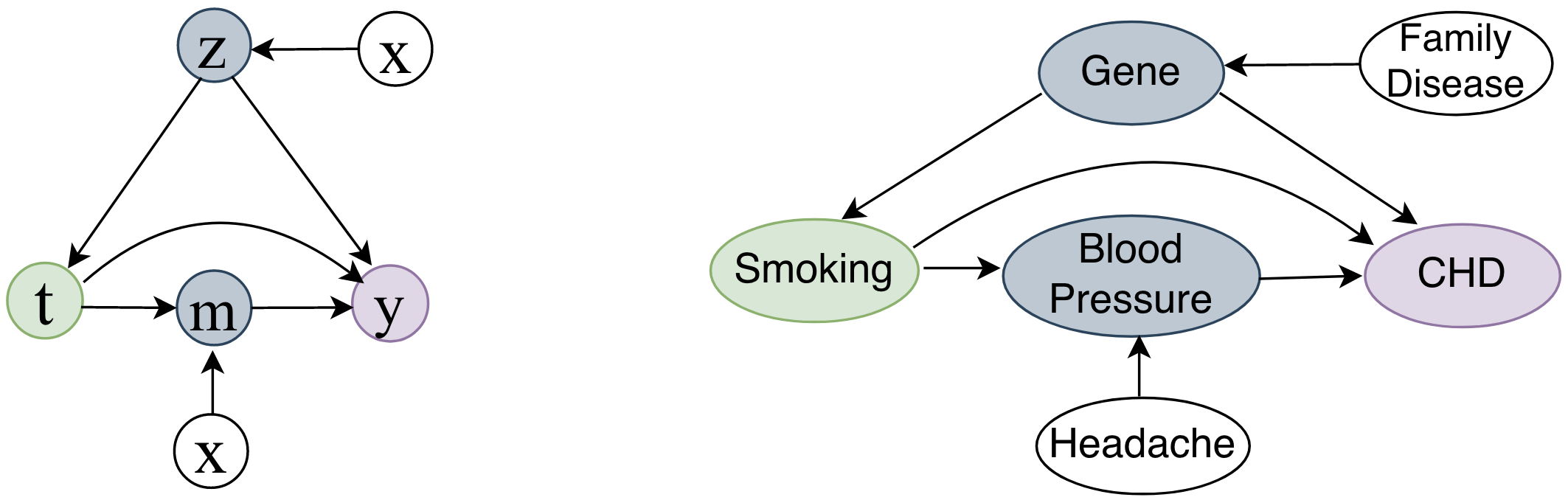
Figure 1: The causal graph with the mediate variable and its example. The confounder $z$ and the mediate variable $m$ in grey are unmeasured in observational study. We can observe some covariates $x$ that are in fact noisy views of $z$ and $m$, such as the headache and family heart disease.

In this work, we propose an end-to-end deep treatment-adaptive network (DTANet) to estimate the treatment effect as shown in Figure 3. To the best of our knowledge, the proposed DTANet is the first representation based method that can quantify the mediate effect transmitted by the change of treatment.

• By a novel orthogonality projection, a mediate feature representation can be learnt to capture the informative treatment-specific variations underlying the unobserved mediate variables. The mediate feature representation independent of unobserved confounders can generate an unbiased estimation of the mediate treatment effect.

• Our DTANet leverages the optimal transport theory to learn a treatment-invariant representation that can alleviate the confounders bias. Moreover, the learned treatment-invariant features can be employed as the off-the-shelf knowledge in estimating causal effect on out-of-samples.

• Finally, DTANet is an end-to-end deep joint network with two separate “heads” for two potential outcomes, by using both the confounding representation and the mediate feature representation. We also prove that the causal effect can be identified from the observational data by DTANet.

2 Background

This section introduces the preliminary knowledge and related work in the field of observational studies.

2.1 The Rationality of Causal Inference

The goal of causal inference is to estimate the causal effect of an intervention/treatment. Randomized controlled trials (RCTs) are now the gold standard for causal inference in medicine and social science. In RCTs, individuals are receiving treatment or controlled treatment by randomization. RCTs allow to estimate the treatment effect by directly comparing the results from assigning the intervention of interest to the results from a “control” intervention. For example, researcher in medicine are interested in assessing the effect of smoking on the health outcome. RCTs assign individuals randomly with smoking and non-smoking. Due to randomization and given a large enough study enrollment, the two study groups (smoking and non-smoking) are fully comparable. That means they will have roughly the same number of individuals at baseline and the same number of individuals in each age (or gender/occupation/etc.) group. The only differences between the two groups should be due to the assignment, all other things (e.g., gender, age, occupation, etc.) having been made equal. Therefore, a direct comparison between two groups’ average health outcome is thus a valid effect estimation of the smoking vs. non-smoking. However, performing RCTs would be neither feasible in behavioral and social science research due to practical or ethical barriers. Because it is impossible to assign people chosen at random to smoke for decades.

Observational studies (or non RCTs) that do not impose any intervention of the individuals’ treatment resort to purely observational data. Unlike the randomized control trials, the mechanism of treatment assignment in observational studies is not explicit. For example, instead of randomized experiments, individuals take smoke based on several factors rather than being assigned randomly. As a result, the distribution of smoking group will generally be different from the non-smoking group. A direct comparison between the health outcomes for smokers and the health outcomes for nonsmokers is no longer valid for estimating the effect of smoking on health outcomes. In this situation, causal inference that is capable of estimating causal effects from observational study are of paramount importance.

2.2 Potential Outcome Framework

Two well-known fundamental causal paradigms, including the potential outcome framework rosenbaum1983central and structural causal models pearl2009causal ; pearl2016causal , are adopted in causal inference from observational studies. In this paper, we focus on the potential outcome framework. The potential outcome framework rosenbaum1983central proposed by Neyman and Rubin has developed into a well-known causal paradigm for treatment effect estimation in observational studies. Considering binary treatments for a set of individuals, there are two possible outcomes for each individual. In general, the potential outcome framework predicts counterfactual (i.e., outcome under an alternative treatment) for each treated individual, and computes the difference between the counterfactual and the factual (observed outcome).

Formally, for an observational dataset $\{\boldsymbol{x}_{i},t_{i},y_{i}\}_{1\leq i\leq n}$ of $n$ individuals, variable $\boldsymbol{x}_{i}\in\mathbb{R}^{n\times d}$ is the $d$-dimensional covariate of individual $i$, and treatment $t_{i}$ affects the outcome $y_{i}$. Considering the binary treatment case, individual $i$ will be assigned to the control group if $t_{i}=0$, or to the treated group if $t_{i}=1$. The individual treatment effect (ITE) is defined as the difference between potential outcomes of an individual under two different treatments:

$$\centering\operatorname{ITE}_{i}=\mathbb{E}(\mathbf{y}_{i}(1))-\mathbb{E}(\mathbf{y}_{i}(0))\@add@centering$$ (1)

Clearly, each individual only belongs to one of these two groups, and therefore, we can only observe one of two possible outcomes. In particular, if individual $i$ is in treated group, $y_{i}(1)$ is the observed/factual outcome, and $y_{i}(0)$ is missing data, i.e., counterfactual. The challenge to estimate ITE lies on how to estimate the missing counterfactual outcome $y_{i}(0)$ by intervening $t=0$.

The potential outcome framework usually makes the following assumptions imbens2000role ; lechner2001identification to estimate the missing counterfactual outcome.

Assumption 1 (Ignorability)

Conditional on the covariates $\boldsymbol{x}$, two potential outcomes are independent of the treatment, i.e. $y_{i}(1),y_{i}(0)\perp t\mid\boldsymbol{x}$.

Assumption 2 (Positivity)

For any set of covariates $\boldsymbol{x}$, the probability of receiving each treatment $a$ is positive, i.e., $0<p(t=a\mid x)<1$.

Estimating causal effects from observational data is different from classic learning because we never see the ground-truth individual-level effect in practice. For each individual, we only see their response to one of the possible actions - the one they had actually received.

2.3 Confounders and Bias

The problem of calculating ITE is translated into the task of estimating the counterfactual outcome under an intervention on treatment. Hence, the potential outcome framework introduces a mathematical operator called $do$-calculus $do(t)$ to define hypothetical intervention on the treatment $t$ pearl2009causality . Specifically, $do(t)=1$ simulates an intervention by setting $t=1$, which indicates that $t$ is only determined by $do$ thus renders $t$ independent of the other variables.

Definition 1 (Interventional Distribution)

The interventional distribution $p(y\mid do(t^{\prime}))$ denotes the distribution of the variable $y$ when we rerun the modified data-generation process where the value of variable $t$ is set to $t^{\prime}$.

For example, for the causal graph in Figure 1, the post-intervention distribution $p(y\mid do(0))$ refers to the distribution of CHD outcome $y$ as if the smoking treatment $t$ is set to $0$ (e.g. non-smoking) by intervention, where all the arrows into $t$ are removed. However, the interventional distribution $p(y\mid do(t^{\prime}))$ is different from observational distribution $p(y\mid t^{\prime})$ due to the existence of confounders.

Definition 2 (Confounders)

Given a pair of treatment and outcome $(t,y)$, we say a variable $z$ is a confounder iff $z$ affects both $t$ and $y$.

Confounder is a common causes of the treatment and outcome. The confounder variable affects the assignment of individuals’ treatment and thus leads to the confounding bias. In the medicine example, gene is a confounder variable, so that people with different gene have different preferences on smoking or not. The probability distribution $p(y|t)$ not only includes the effect of treatment on the outcome (i.e., $p(y\mid do(t))$), but also includes the statistical associations produced by confounders on the outcome, which leads to the spurious effect. Consequently, confounders render the probability distribution $p(y\mid t)$ and intervention distribution $p(y\mid do(t))$ distinct, which makes calculating ITE more difficult.

Definition 3 (Confounding Bias)

Given variables $x$, $y$, confounding bias exists for causal effect $t\rightarrow y$ iff the observational probabilistic distribution is not always equivalent to the interventional distribution, i.e., $p(y\mid t)\neq p(y\mid do(t))$.

Confounding bias in observational study is equivalent to a domain adaptation scenario where a model is trained on a “source” (observed) data distribution, but should perform well on a “target” (counterfactual) one. Handing confounding bias is the essential part of causal inference, and the procedure of handing confounder variables is called adjust confounders.

3 Related work

Estimation of individual treatment effect in observational data is a complicated task due to the challenges of confounding bias xu2020causality ; pearl2009causality ; dung2021stochastic . Unlike the randomized control trials, the mechanism of treatment assignment is not explicit in observational data due to the confounding bias. Therefore, interventions of treatment are not independent of the property of the subjects, which results in the difference between the intervention (i.e., counterfactual) distribution and the observed distribution. To predict counterfactual outcomes from the factual data, many practical solutions are proposed to adjust confounders, which can be classified into four categories.

A common statistical solution is re-weighting certain data instances to balance the observed distribution and intervention distributions caused by confounding bias problem (as described in Section 2.3). Apparently, confounding bias leads to the fact that treatment assignment is not random but is correlated with covariates. By defining an appropriate weight as the function of covariates to each individual in the observational data, a pseudo-population can be created on which the distributions of the treated group and control group are similar. In other words, the treatment assignment is synthesized to be random after weighting individuals. The majority of re-weighting approaches belong to the Inverse Propensity Weighting (IPS) family of methods austin2011introduction . Here, the propensity denotes the estimated probability of receiving a treatment rosenbaum1983central , which is often modelled by a logistic regression of treatment on the covariates. IPS weights the individuals with inverse propensity to make a synthetic random treatment assignment and further create unbiased estimators of treatment effect.

Methods in the second category is matching, which provides a way to estimate the counterfactual while reducing the confounding bias brought by the confounders. According to the (binary) treatment assignments, a set of individuals can be divided into a treatment group and a control group. For each treated individual, matching methods select its counterpart in the control group based on certain criteria, and treat the selected individual as a counterfactual. Then the treatment effect can be estimated by comparing the outcomes of treated individuals and the corresponding selected counterfactuals. Various distance metrics have been adopted to compare the closeness between individuals and select counterparts. Some popular matching estimators include nearest neighbor matching (NNM) rubin1973matching , propensity score matching rosenbaum1983central , and genetic matching diamond2013genetic , etc. In detail, a propensity score measures the propensity of individuals to receive treatment given the information available in the covariates. In Figure 1, we can estimate the propensity score by fitting a logistic model for the probability of quitting smoking conditional on the covariates. Propensity score methods match each treated individual to the controlled individual(s) with the similar propensity score (e.g., one-to-one or one-to-many), and then treat the matched individual(s) as the controlled outcome diamond2013genetic ; bang2005doubly . The individual treatment effect equals to the difference between the matched pair of the treated individual and the controlled individual.

Methods in the third category learn individualized treatment effects (ITE) via parametric regression models to exploit the correlations among the covariates, treatment and outcome. Bayesian Additive Regression Trees (BART) hill2011bayesian , Causal Random Forest (CF) wager2018estimation and Treatment-Agnostic Representation Network (TARNet) shalit2017estimating are typical methods of this category. In particular, BART in hill2011bayesian applies a Bayesian form of boosted regression trees on covariates and treatment for estimating ITE, and it is capable of addressing non-linear settings and obtain more accurate ITE than the propensity score matching and inverse probability of weighting estimators hill2011bayesian . Causal random forest (CF) views forests as a adaptive neighbourhood metric and estimates the treatment effects at the leaf node wager2018estimation . TARNet shalit2017estimating is a complex deep model that builds on learning non-linear representations between the covariates and potential outcomes. Doubly Robust Linear Regression (DR) dudik2011doubly combines the propensity score weighting with the outcome regression, so that the estimator is robust even when one of the propensity scores or outcome regression is incorrect (but not both).

The fourth category has predominantly focused on learning representations regularized to balance these confounding factors by enforcing domain invariance with distributional distances johansson2016learning ; schwab2018perfect . The big challenge in treatment effect estimation is that the intervention distribution is not identical to the observed distribution, which converts the causal inference problem to a domain adaptation problem li2021hilbert ; li2015lingo . Building on this work johansson2016learning , the discrepancy distance between distributions is tailored to adaptation problems. An intuitive idea is to enforce the similarity between the distributions of different treatment groups in the representation space. Two common discrepancy metrics in this area are used: empirical discrepancy by Balancing Neural Network (BNN) johansson2016learning and maximum mean discrepancy by Counterfactual Factual Regression Network (CFRNet) shalit2017estimating . Particularly, BNN learns a balanced representation that adjusts the mismatch between the entire sample distribution and treated and control distributions in order to account for confounding bias. CFRNet provides an intuitive generalization-error bound. The expected ITE representation error is bounded by the generalization-error and the distribution distance. The drawback of methods in this category is that they overlooks the important information that can be estimated from data: the treatment/domain assignment probabilities johansson2018learning .

4 Problem Formulation

4.1 Motivation

Treatment can cause the outcome directly or indirectly through mediation (e.g., blood pressure). The indirect cause is largely unexploited by most of the previous representation methods, which leads to the biased estimation of treatment effect. In this paper, we consider the causal graph in Figure 1 with confounder and mediate variable. Both the confounder and the mediate variable may not be amenable to direct measurements. It is reasonable to assume that both the confounder and the mediate variable can be reliably represented by a set of covariates for each individual. For example, even if the family gene and blood pressure can not be measured directly, they can also be reflected by the family disease and the headache as shown in Figure 1. We will prove that true treatment effect in Figure 1 can be identified from observations by our DTANet.

4.2 Theoretical Results

We admit the existence of mediate variable and consider the causal graph in Figure 1. Next, we define the potential outcomes. Previously, the potential outcomes were only a function of the treatment, but in our scenario the potential outcomes depend on the mediate variable as well as the treatment variable. Assume $m(t_{i})$ is the mediate variable under the treatment status $t_{i}$, and $z$ is the unobserved confounder. The mediate variable is a post-treatment variable and can be changed by the intervention on treatment. This change will further affect the outcome, which results in the bias between the interventional distribution and observed distribution as

$$p(y_{i}\mid do(t=1),m_{i}(t),x_{i})\neq p(y_{i}\mid t=1,m_{i},x_{i})$$ (2)

In this case, the bias will lead to invalid ITE in Eq. (1). Consequently, extracting the mediate variable from the covariates is vital for the unbiased the treatment effect estimation.

Our goal is to estimate ITE under the existence of mediate variable. We reformulated ITE defined in Eq. (1) as Eq. (3) and prove that it is be identified from observations.

$$\begin{split}\tau_{ITE}(\boldsymbol{x})=\mathbb{E}[y(t,m(t))\mid\boldsymbol{x},do(t=1)]\\ -\mathbb{E}[y(t,m(t))\mid\boldsymbol{x},do(t=0)]\end{split}$$ (3)

Theorem 4.1

The causal effect defined by ITE in Eq. (3) can be identified from the distribution $p(\boldsymbol{x},t,y)$.

Proof

ITE can be non-parametrically identified by

$$\begin{split}&p(y(t,m(t))\mid\boldsymbol{x},do(t=1))\\ &=\int_{m}p(\mathbf{y}\mid\boldsymbol{x},m)p(m\mid\boldsymbol{x},do(t=1))dm\\ &\stackrel{{\scriptstyle[}}{{]}}{(i)}{=}\int_{m}p(\mathbf{y}\mid\boldsymbol{x},m)p(m\mid\boldsymbol{x},t=1)dm\\ &=\int_{m}\int_{z}p(\mathbf{y}\mid\boldsymbol{x},z,m)p(z\mid\boldsymbol{x},m)p(m\mid\boldsymbol{x},t=1)dmdz\\ &\stackrel{{\scriptstyle[}}{{]}}{(ii)}{=}\int_{m}\int_{z}p(\mathbf{y}\mid z,m)p(z\mid\boldsymbol{x})p(m\mid\boldsymbol{x},t=1)dmdz\end{split}$$ (4)

According to Figure 1, there is no common cause between the treatment and the mediate variable. Therefore, the interventional distribution $p(m\mid\boldsymbol{x},do(t=1))$ equals the observed distribution $p(m\mid\boldsymbol{x},t=1)$, which allows equality (i) in Eq. (4) to be satisfied. As indicated by Figure 1, when the confounder $z$ is conditioned, $y$ is independent of $x$, i.e., $y\perp\boldsymbol{x}\mid z$. Similarly, $z$ is independent of $m$ when $\boldsymbol{x}$ is conditioned, i.e., $z\perp m\mid\boldsymbol{x}$. The equality (ii) holds because of $y\perp\boldsymbol{x}\mid z$ and $z\perp m\mid\boldsymbol{x}$. The final expression only depends on the distribution $p(\boldsymbol{x},z,m,t,y)$. Similarly, we can also prove that $p(\mathbf{y}(t,m(t))\mid\boldsymbol{x},do(t=1))$ can be expressed by observations $p(\boldsymbol{x},z,m,t,y)$. Based on ITE in Eq. (3), we can conclude that ITE can be computed by recovering the distribution $p(\boldsymbol{x},z,m,t,y)$ from the observational dataset $(\boldsymbol{x},t,y)$.

4.3 Representation Learning for $z$ and $m$

Identification of treatment effects relies on causal assumptions, which can be encoded in a causal graph. This is the fundamental assumption for causal inference methods. In this paper, we design a representation based causal graph shown in Figure 2, based on which we propose deep treatment-adaptive network (DTANet) for treatment effect estimation. Our method is based on the same causal graph that is widely used by previous causal inference methods, i.e., $(T\leftarrow Z\rightarrow Y,T\rightarrow Y)$. In addition, we extend this causal graph by involving the existence of $m$ between $t$ and $y$. DTANet learns the latent confounding representation and the mediate feature representation for the unmeasured confounders $z$ and mediate variables $m$, respectively. As proved in theorem 4.1, conditioning on the $z$ and $m$ would amplify the treatment effect estimation bias. Defining proxy variables for unmeasured $z$ and $m$ requires domain-specific prior knowledge that is not easy to obtain. Consequently, our task is to learn two latent representations to filter out the information related to $z$ and $m$ from covariates, which requires no prohibitive assumption or knowledge on unobserved $z$ and $m$.

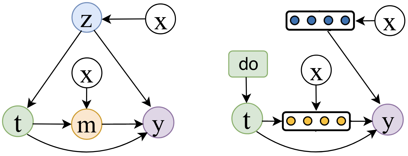
Figure 2: The representation based causal graph for unobserved confounder $z$ and mediate variable $m$.

Debiasing confounder $z$. The confounding representation is learned from covariates with the aim of alleviating the confounding bias. The treatment assignment is not randomly but typically biased by the confounder. For example, poor patients are more likely to choose the cheap treatment, where the economic status as a confounder determines the choice of treatment. The distribution of individuals may therefore differ significantly between the treated group and the overall population. A supervised model naïvely trained to minimise the factual error would overfit to the properties of the treated group, and thus not generalise well to the entire population.

According to theorem 4.1, inferring causal effect would be straightforward if the confounder $z$ is available. So, as the substitute for the unknown confounder, we would like to learn a treatment-invariant representation from the observed covariates. We justify the rationality of this strategy based on: 1) as the confounder is hidden in the observable covariates, i.e., the family gene is hidden in the family disease, confounder can be learned from covariates; 2) as $do$-calculus removes the dependence of treatment on confounder shown in Figure 2, the substitution of the confounder should capture the generalized or mutual information of covariates, i.e., treatment-invariant property. The learned representation with treatment-invariant property containing the covariate features such that the induced distributions of individuals under different treatments look similar, which can thus generalize well to the entire population.

Mediate feature learning for $m$. Previous representation based models neglect the interactions between the treatment and the individuals’ covariates, i.e., doing different interventions on the treatment may result in varied mediate treatment effects that can further change the observed covariates as well. Neglecting such change in the observed covariates will lead to serious bias for the treatment effect estimation, as the confounding representation is learned from the static covariates. Namely, some covariates are in fact mediate variables that can be changed by a different treatment value. To capture the dynamic changes private to different treatments, we learn a mediate feature representation of unobserved mediate variables.

4.4 Causal Quantities of Interest

The treatment effect can be measured at the individual level and group level.

4.4.1 Individual Level

The key quantity of interest in causal inference is treatment effect on outcome. Based on ITE in Eq. (3) and Theorem 4.1, we have ITE for each individual $i$ as

$$\tau_{{ITE}_{i}}=y_{i}(1,m_{i}(1),\boldsymbol{x}_{i})-y_{i}(0,m_{i}(0),\boldsymbol{x}_{i})$$ (5)

where $y_{i}(1,m_{i}(1),\boldsymbol{x}_{i})$ is the treated outcome of individual $i$ after applying $do(t_{i})=1$, $m_{i}(1)$ is the mediate variable resulting from $do(t_{i})=1$ and $\boldsymbol{x}_{i}$ is the covariate vector. Similar to treated outcome, $y_{i}(0,m_{i}(0),\boldsymbol{x}_{i})$ is the controlled outcome after applying $do(t_{i})=0$.

We define the Mediate Treatment Effect (MTE) to quantify the effect of treatment on outcome that occurs through a mediate variable.

$$\tau_{{MTE}_{i}(t)}=y_{i}(t,m_{i}(1))-y_{i}(t,m_{i}(0))$$ (6)

Note that $\tau_{MTE}$ is computed by applying $do$-calculus on $m$ and keeping $t$ unchanged. The key to understanding Eq. (6) is the following counterfactual question: What change would occur to the outcome if one changes $m$ from $m(0)$ to $m(1)$, while holding the treatment status at $t$? If the treatment $t$ has no effect on the $m$ , that is, $m(0)\neq m(1)$, then the mediate treatment effect is zero.

We also are interested in Direct Treatment Effect that computes how much of the treatment variable $t$ directly affects the outcome $y$. Similarly, we can define the individual direct effect of the treatment as follows:

$$\tau_{{DTE}_{i}(t)}=y_{i}(1,m_{i}(t))-y_{i}(0,m_{i}(t))$$ (7)

which denotes the direct causal effect of the treatment on the outcome other than the one represented by the mediate variable. Here, the mediate variable is held constant at $m_{i}(t)$ and the treatment variable is changed from zero to one.

Finally, the sum of (6) and (7) equals (5), which formally decomposes ITE into Mediate Treatment Effect and Direct Treatment Effect as follows.

$$\tau_{{ITE}_{i}}=\tau_{{MTE}_{i}(t)}+\tau_{{DTE}_{i}(1-t)}$$ (8)

4.4.2 Population Level

Given these individual-level causal quantities of interest, we can define the population average effect for each quantity. At the population level, the individual treatment effect is named as the Average Treatment Effect (ATE), which is defined as:

$$\begin{split}\tau_{ATE}&=\frac{1}{n}\sum_{i}^{n}\left(y_{i}(1,m_{i}(1))-y_{i}(0,m_{i}(0))\right)\\ &=\frac{1}{n}\sum_{i}^{n}\tau_{{ITE}_{i}}\end{split}$$ (9)

Suppose we have $n_{t}$ treated individuals, Average Treatment effect on the Treated group (ATT) is defined as

$$\tau_{ATT}=\frac{1}{n_{t}}\sum_{i}^{n_{t}}\tau_{ITE}(i|t=1)$$ (10)

where $n_{t}$ is the number of individuals having $t=1$, i.e., the treated group size. Here, $\tau_{ITE}(i|t=1)$ is ITE for individual $i$ from the treated group.

Similarly, we define average Mediate Treatment Effect and Direct Treatment Effect as

$$\tau_{AME}=\frac{1}{n}\sum_{i}^{n}\tau_{MTE}(i),\quad\tau_{ADE}=\frac{1}{n}\sum_{i}^{n}\tau_{DTE}(i)$$ (11)

5 Methodology

In this section, we learn the representations for unmeasured $z$ and $m$ given in Figure 2 in order to compute the individual treatment effect (ITE) of Eq. (3). We propose a novel deep treatment-adaptive network (DTANet) as shown in Figure 3. Particularly, DTANet can jointly learn the unbiased confounding representation for $z$ by the optimal transport. Moreover, the mediate features of $m$ viewed as treatment-specific variations can be guaranteed by the proposed orthogonal projection constraint. The confounding representation is concatenated with mediate feature representation for the potential outcome predictor network. With two potential outcomes, the individual treatment effect (ITE) can be estimated by Eq. (3).

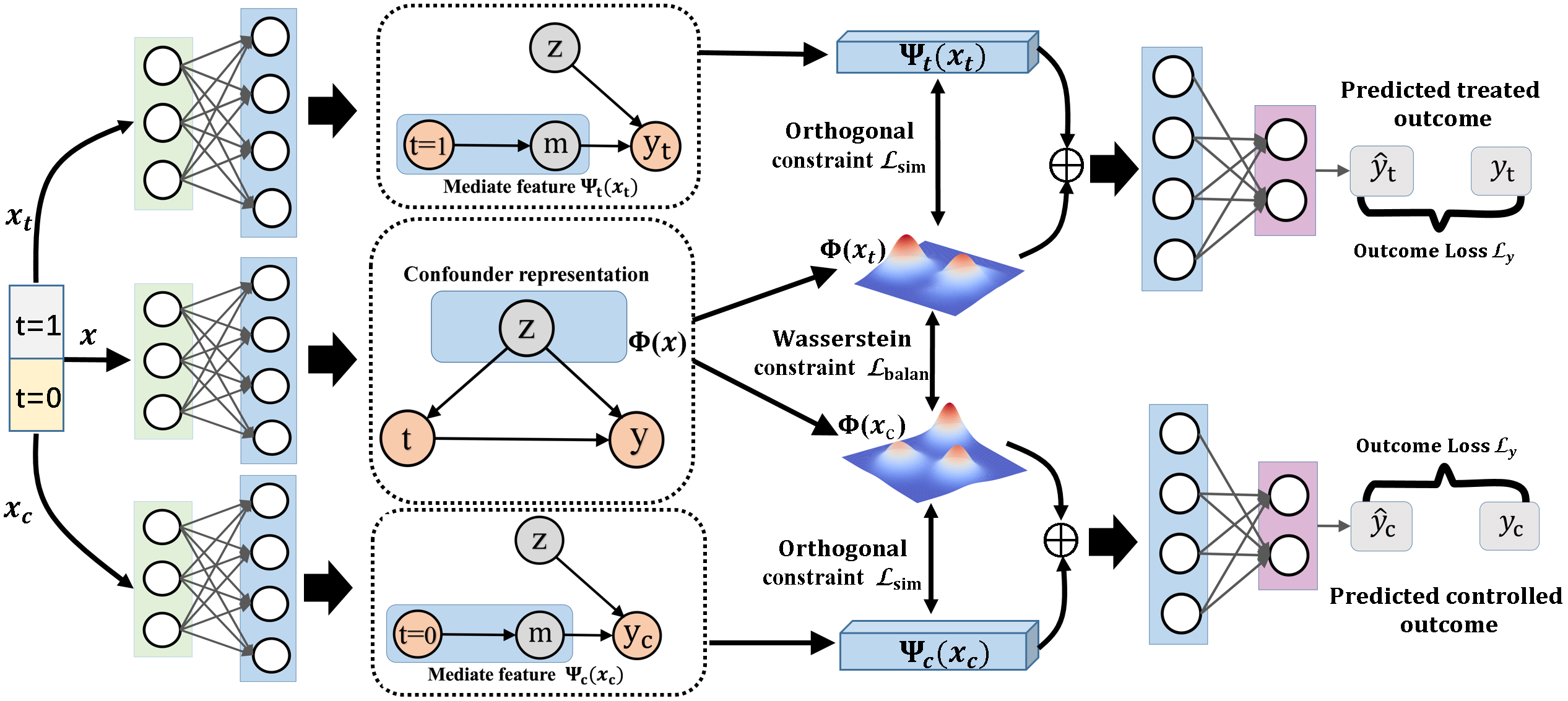
Figure 3: Our DTANet method provides an end-to-end procedure for predicting potential outcomes from covariates $\boldsymbol{x}$, which can be further used for estimating treatment effect. A confounding representation network $\Phi(\cdot)$, two mediate feature representation networks ($\Psi_{t}(\cdot)$ and $\Psi_{c}(\cdot)$) and two predictors of potential outcomes together form DTANet.

5.1 Debiasing Confounder by Optimal Transport

Motivated by the intuition in Section 4.3, we define $z=\Phi(;W):\mathcal{X}\rightarrow\mathcal{Z}$ as the representation network for the common confounding information between the treated individuals and the controlled individuals. The network $\Phi(;W)$ has $L$ layers with weight parameters $W$ by

$$\Phi(\boldsymbol{x};W)=f_{L}(\ldots f_{1}(w_{(1)}^{\top}\boldsymbol{x})\ldots)$$ (12)

where $f_{1}\cdots f_{L}$ are nonlinear activation functions, $w_{(1)}^{\top}x$ is an affine transformation map controlled by weight parameters $w_{1}$ for first layer, and $W=\{w_{(1)},\cdots,w_{(L)}\}$ is the weight matrix for $L$-th layers.

According to the binary treatment setting, an individual in the observational dataset can be either a treated or controlled individual. To allow $\Phi$ to satisfy the treatment-invariant property, we adopt the optimal transport villani2008optimal ; peyre2019computational ; li2021hilbert ; courty2014domain ; wang2019polynomial to minimize the discrepancy introduced by $\Phi$ between the distribution of treated and controlled individuals. We use $\boldsymbol{x}_{t}$ for the treated covariates and $\boldsymbol{x}_{c}$ for the controlled covariates. $p(\Phi(\boldsymbol{x}_{t}))$ and $q(\Phi(\boldsymbol{x}_{c}))$ are the treated and the controlled distribution induced by $\Phi(\cdot)$. We resort to optimal transport theory that allows to use Wasserstein distance peyre2019computational on the space of probability measures $p(\Phi(\boldsymbol{x}_{t}))$ and $q(\Phi(\boldsymbol{x}_{c}))$. Wasserstein metric incorporates the underlying geometry between outcomes, which can be applied to distributions with non-overlapping supports, and has good out-of-sample performance esfahani2018data . We apply the Wasserstein distance to reduce the discrepancy even with limited or no overlap between $p(\Phi(\boldsymbol{x}_{t}))$ and $q(\Phi(\boldsymbol{x}_{c}))$.

Definition 4

Given a hypothesis set $\mathcal{H}$, the Wasserstein distance between $p_{\Phi}$ and $q_{\Phi}$ is

$$\mathcal{W}_{2}(p_{\Phi},q_{\Phi})=\left(\inf_{\pi\in\Pi}\int_{\Omega}d\left(\Phi(\boldsymbol{x}_{t}),\Phi(\boldsymbol{x}_{c})\right)d\pi\right)^{\frac{1}{2}}$$ (13)

where set $\Pi$ is the joint probability measures on $\Omega=\Phi(\boldsymbol{x}_{t})\times\Phi(\boldsymbol{x}_{c})$ with marginal probabilities $p_{\Phi}$ and $q_{\Phi}$.

As both $p_{\Phi}$ and $q_{\Phi}$ have finite supports, we will only consider Wasserstein distance for discrete distributions. Given realizations $\{\boldsymbol{x}_{t_{i}}\}_{i=1}^{n_{t}}$ and $\{\boldsymbol{x}_{c_{j}}\}_{j=1}^{n_{c}}$, we reformulate Eq. (13) on two discrete empirical distributions $p_{\Phi}$ and $q_{\Phi}$ w.r.t. treatment individuals and control individuals, i.e.,

$$p_{\Phi}=\frac{1}{n_{c}}\sum_{i=1}^{n_{c}}\delta_{i},\quad q_{\Phi}=\frac{1}{n_{t}}\sum_{j=1}^{n_{t}}\delta_{j}$$ (14)

Minimizing the discrepancy between $p_{\Phi}$ and $q_{\Phi}$ with Wasserstein distance is equivalent to solving the optimization

$$\mathcal{W}_{2}(p_{\Phi},q_{\Phi}):\stackrel{{\scriptstyle\text{ def }}}{{=}}\min_{\boldsymbol{\gamma}\in\mathbf{U}}\left\langle\mathbf{C}_{\Phi},\boldsymbol{\gamma}\right\rangle_{F}$$ (15)

where $\langle\cdot,\cdot\rangle_{F}$ is the Frobenius dot-product of matrices. The optimal $\boldsymbol{\gamma}$ belongs to

$$\mathbf{U}=\left\{\boldsymbol{\gamma}\in\mathbb{R}_{+}^{n_{c}\times n_{t}}\mid\boldsymbol{\gamma}\boldsymbol{1}_{n_{t}}=p_{\Phi},\boldsymbol{\gamma}^{\top}\boldsymbol{1}_{n_{c}}=q_{\Phi}\right\}$$ (16)

that refers to non-negative matrices such that their row and column marginals are equal to $p_{\Phi}$ and $q_{\Phi}$ respectively. The distance matrix between $\boldsymbol{x}_{t}$ and $\boldsymbol{x}_{c}$ is $\mathbf{C}_{\Phi}\in\mathbb{R}^{n_{c}\times n_{t}}$ with element

$$\mathbf{C}_{ij}=\|\Phi(\boldsymbol{x}_{c_{i}};W)-\Phi(\boldsymbol{x}_{t_{j}};W)\|^{2}_{2}$$ (17)

Hence, we propose Eq. (15) as the loss $\mathcal{L}_{balan}$ that reduces the discrepancy between the treated and control individuals, i.e.,

$$\mathcal{L}_{balan}=\min_{\boldsymbol{\gamma}\in\mathbf{U}}\left\langle\mathbf{C}_{\Phi},\boldsymbol{\gamma}\right\rangle_{F}$$ (18)

Solving $\mathcal{L}_{balan}$ ensures the treatment-invariant representation $\Phi$ is similar across different treatment values and thus is independent of the treatment assignment. The confounding representation provides more stable gradients even if two distributions of treated and controlled individuals are distant, as well as informative for treatment effect estimation. Moreover, since treatment-invariant features are independent of the treatment assignment, they can be considered as off-the-shelf knowledge and used to estimate causal effect on out-of-samples.

5.2 Orthogonal Projection for Mediate Features Learning

According to the binary treatment assignments, individuals in the observational dataset can be either divided into the treated individuals or the controlled individuals. We design two mediate feature representations encoding different treatment-specific variations private to both populations (i.e., the treated individuals and the controlled individuals). Moreover, the confounder is no long correlated with the treatment after $do$ intervention as shown in causal graph Figure 3. Thus, a soft orthogonal projection term is also proposed to separate the mediate features from the confounding representation as much as possible. This guarantees the confounding representation is pure and not contaminated by treatment.

Similar to representation by Eq. (12), let functions $\Psi(\boldsymbol{x}_{t};V_{t})$ and $\Psi(\boldsymbol{x}_{c};V_{c})$ map treated individuals $\boldsymbol{x}_{t}$ and controlled individuals $\boldsymbol{x}_{t}$ to hidden mediate representations specialised in each domain.

$$\begin{split}\Psi_{t}(\boldsymbol{x}_{t};V_{t})=f_{L}(\ldots f_{1}(v_{t_{(1)}}^{\top}\boldsymbol{x}_{t})\ldots),\vspace{1pt}\\ \Psi_{c}(\boldsymbol{x}_{c};V_{c})=f_{L}(\ldots f_{1}(v_{c_{(1)}}^{\top}\boldsymbol{x}_{c})\ldots),\vspace{1pt}\end{split}$$ (19)

where $V_{t}=[v_{t_{(1)}}\cdots v_{t_{(L)}}]$ and $V_{c}=[v_{c_{(1)}}\cdots v_{c_{(L)}}]$ are weight matrices for $L$-layers of the treated and controlled representation, respectively.

We propose an orthogonality constraint for the loss $\mathcal{L}_{sim}$ to separate the confounding representation from mediate representation. Let $Z_{t}$ and $Z_{c}$ be matrices whose rows are the outputs of confounding representation $\Phi(\cdot)$ from treated $\boldsymbol{x_{t}}$ and controlled individuals $\boldsymbol{x_{c}}$, respectively. Similarly, let $M_{t}$ and $M_{c}$ be matrices whose rows are the outputs of the mediate feature representation $\Psi_{t}(\boldsymbol{\cdot})$ and $\Psi_{c}(\boldsymbol{\cdot})$, respectively. Mathematically, we have

$$\begin{split}\mathcal{L}_{sim}&=\|M_{t}^{\top}Z_{t}\|_{F}^{2}+\|M_{c}^{\top}Z_{c}\|_{F}^{2}\end{split}$$ (20)

where $\|\cdot\|_{F}^{2}$ is the squared Frobenius norm. The loss function $\mathcal{L}_{sim}$ encourages $\Psi_{t}(\cdot)$ and $\Psi_{c}(\cdot)$ to encode discriminative features that are specific to their own domain. As $\Psi_{t}(\cdot)$ and $\Psi_{c}(\cdot)$ are deduced by the specific treatment, $\Phi(\cdot)$ is constrained to be as general as possible irrespective of the treatment information.

5.3 Joint Two-headed Networks for Outcome Prediction

Parametrizing two potential outcomes with a single network as in johansson2016learning is not optimal, because the influence of $t$ on the potential outcome might be too minor to lost during the training for the high-dimensional case of $\Phi$. We construct two separate “heads” of the deep joint network $\hat{y}_{t}$ and $\hat{y}_{c}$ for the two potential outcomes under treatment and control, as indicated in Figure 3. The concatenation of $[\Phi(\cdot),\Psi_{t}(\cdot)]$ or $[\Phi(\cdot),\Psi_{c}(\cdot)]$ is ultimately fed into the potential outcome network $\hat{y}_{t}$ or $\hat{y}_{c}$, respectively. Namely, each sample is used to update only the head corresponding to observed treatment.

$$\hat{y}_{t}(\Phi,\Psi_{t};\Theta_{t}) =f_{L}(\ldots f_{1}(\theta_{t}^{\top}(\Phi(\boldsymbol{x}_{t}),\Psi_{t}(\boldsymbol{x}_{t})))\ldots)$$ (21)

$$\hat{y}_{c}(\Phi,\Psi_{c};\Theta_{c}) =f_{L}(\ldots f_{1}(\theta_{c}^{\top}(\Phi(\boldsymbol{x}_{c}),\Psi_{c}(\boldsymbol{x}_{c})))\ldots)$$

where $\Theta_{t}=[\theta_{t_{(1)}}\cdots\theta_{t_{(L)}}]$ and $\Theta_{c}=[\theta_{c_{(1)}}\cdots\theta_{c_{(L)}}]$ are weight matrices for $L$ layers of the treated and the controlled, $f_{1}(\cdot)$ is the first layer with the linear transformation weight $\theta_{t}$ or $\theta_{c}$ for the treated group or the controlled group, respectively. Minimizing the loss function $\mathcal{L}_{y}$ to approximate two predicted potential outcomes to the ground-truths.

$$\mathcal{L}_{y} =\frac{\lambda_{0}}{n_{t}}\sum_{i=1}^{n_{t}}\|\hat{y}_{t_{i}}-y_{t_{i}}\|_{2}^{2}+\frac{1-\lambda_{0}}{n_{c}}\sum_{j=1}^{n_{c}}\|\hat{y}_{c_{j}}-y_{c_{j}}\|_{2}^{2}$$ (22)

where $\lambda_{0}$ is a hyper parameter compensating for the difference between the sizes of treated samples and controlled samples. With the fitted models $\hat{y}_{t}$ and $\hat{y}_{c}$ parametrized by $\Phi,\Psi_{t}$ and $\Psi_{c}$ in hand, we can estimate the individual treatment effect (ITE) as

$$\tau_{ITE}(i)=\hat{y}_{t_{i}}-\hat{y}_{c_{i}}$$ (23)

Remark. The mediate feature learning component enables our approach to estimate the mediate treatment effect at the presence of mediate variable. Our approach can also estimate the Direct Treatment Effect where no mediate variable exists in observational data. This scenario implies the treatment $t$ is assumed to have a direct effect on the outcome $y$, i.e., $t\rightarrow y$. In case the prior knowledge of $t\rightarrow y$ is known in practice, our approach can estimate Direct Treatment Effect by merely removing mediate feature learning component. Recall that debiasing confounder adjusts the confounder variables by learning a treatment-invariant representation $\phi(\cdot)$, so that the treatment assignment is independent of the confounding bias. Without mediate variable $m$, $\phi(\cdot)$ is no longer regularized by the orthogonal constraint (20) and becomes an unique cause of the outcomes. Then the learned $\phi(\cdot)$ is directly feed into outcome prediction for inferring treated and controlled outcomes, respectively. Finally, ITE can be computed via Eq. (23).

6 Optimization

We consider the deep feed-forward network that is trained to minimize the final loss function Eq. (24) using mini-batch stochastic gradient descent with the Adam optimizer kingma2014adam . Specifically, we propose an end-to-end algorithm that alternatively trains the parameters of the potential network, the confounder network and the mediate feature representation network with back-propagation.

$$\begin{split}\mathcal{L}=\mathcal{L}_{y}+\lambda_{1}\mathcal{L}_{sim}+\lambda_{2}\mathcal{L}_{balan}\end{split}$$ (24)

where $\lambda_{1}$ and $\lambda_{2}$ are hyper-parameters that control the interaction of the loss terms during learning.

6.1 Updating $\Psi_{t}$ and $\hat{y}_{t}$

Based on Eq. (19) and Eq. (23), the representation $\Psi_{t}$ and outcome $\hat{y}_{t}$ are parametrized by $V_{t}$ and $\Theta_{t}$, respectively. Given the learning rate $\eta$, the gradients of objective function Eq. (24) with respect to parameters $V_{t}$ and $\Theta_{t}$ are

$$\nabla_{V_{t}}\mathcal{L}=\frac{\partial\mathcal{L}_{y}}{\partial\hat{y}_{t}}\frac{\partial\hat{y}_{t}}{\partial V_{t}}+\lambda_{1}\frac{\partial\mathcal{L}_{sim}}{\partial V_{t}},\quad\nabla_{\Theta_{t}}\mathcal{L}=\frac{\partial\mathcal{L}_{y}}{\partial\Theta_{t}}$$ (25)

So the gradient descent updates the corresponding parameters of $\Psi_{t}$ and $\hat{y}_{t}$. The update for $\Psi_{c}$ and $\hat{y}_{c}$ is similar to $\Psi_{t}$ and $\hat{y}_{t}$, since they have similar optimization subproblems.

6.2 Updating $\Phi$

Recall that the confounding representation $\Phi$ in Eq. (12) is parametrized by $W$. Update the confounding representation $\Phi$ is non-trivial due to the existence of optimal transport loss $\mathcal{L}_{balan}$ in Eq. (24). The gradient of $\mathcal{L}$ w.r.t. the $W$ is

$$\begin{split}\nabla_{W}\mathcal{L}=\nabla_{W}\mathcal{L}_{y}+\lambda_{1}\nabla_{W}\mathcal{L}_{sim}+\lambda_{2}\nabla_{W}\mathcal{L}_{balan}\end{split}$$ (26)

To compute the gradient of optimal transport loss $\mathcal{L}_{balan}$, we regularize it by adding a strongly convex term

$$\mathcal{R}(T)=-\frac{1}{\lambda_{3}}\sum_{i,j}T_{i,j}\log\boldsymbol{\gamma}_{i,j}$$ (27)

that is the entropy  benamou2015iterative of $\boldsymbol{\gamma}$. Then, we solve the regularized loss term by the Sinkhorn’s iterations cuturi2014fast

$$\boldsymbol{\gamma}^{k}=\operatorname{diag}(\mathbf{u}^{k})\mathbf{K}\operatorname{diag}(\mathbf{v}^{k})=\mathbf{u}^{k}\mathbf{1}_{n_{t}}^{\top}\circ\mathbf{K}\circ\mathbf{1}_{n_{c}}(\mathbf{v}^{k})^{\top}$$ (28)

where $\circ$ is element-wise multiplication, the element $\mathbf{K}_{i,j}\allowbreak=\exp(-\lambda_{3}\mathbf{C}_{i,j})$ in kernel matrix $K$ is computed based on $\mathbf{C}_{i,j}$ in Eq. (17), and the updates of scaling vectors are

$$\mathbf{v}^{k}=\frac{\mathbf{1}_{n_{t}}/n_{t}}{\mathbf{K}^{\top}\mathbf{u}^{k-1}},\quad\mathbf{u}^{k}=\frac{\mathbf{1}_{n_{c}}/n_{c}}{\mathbf{K}\mathbf{v}^{k}}$$ (29)

Update the pairwise distance matrix between all treated and controlled pairs $C_{\Phi}$ with $W^{k-1}$ by Eq. (17). Then, we have

$$\nabla_{W}\mathcal{L}_{balan}=\frac{\partial\langle\boldsymbol{\gamma}^{k},C_{\Phi}\rangle}{\partial W}$$ (30)

Apparently, the gradients of $\nabla_{W}\mathcal{L}_{y}$ and $\nabla_{W}\mathcal{L}_{sim}$ are

$$\begin{split}&\nabla_{W}\mathcal{L}_{y}=\lambda_{t}\frac{\partial\mathcal{L}_{y}}{\partial\hat{y}_{t}}\frac{\partial\hat{y}_{t}}{\partial W}+\lambda_{c}\frac{\partial\mathcal{L}_{y}}{\partial\hat{y}_{c}}\frac{\partial\hat{y}_{c}}{\partial W}\\ &\nabla_{W}\mathcal{L}_{sim}=\frac{\partial\mathcal{L}_{sim}}{\partial W}\end{split}$$ (31)

With all these computed gradients, the steps of solving Eq. (24) are shown in Alg. 1. Note that the mediate feature representation network and potential outcome network are trained only using the batch with the respective treatment, e.g., the batch of treated individuals for treated features $\Psi_{t}(\cdot)$ and treated outcome $\hat{y}_{t}$.

1:Treated individuals $(\boldsymbol{x}_{t_{i}},y_{t_{i}})_{i=1}^{n_{t}}$ and controlled individuals $(\boldsymbol{x}_{c_{j}},y_{c_{j}})_{j=1}^{n_{c}}$. Adam hyper-parameters $\alpha$, $\beta_{1}$, $\beta_{2}$. scaling parameters $\lambda_{0}$, $\lambda_{1}$, $\lambda_{2}$, $\lambda_{3}$, $\mathbf{u}=\boldsymbol{1}_{n_{c}}$

2:while not converged do

3:     Sample a treated batch $\mathcal{D}_{t}$ and controlled batch $\mathcal{D}_{c}$

4:     Compute $\nabla_{W}\mathcal{L},\nabla_{V_{t}}\mathcal{L},\nabla_{V_{c}}\mathcal{L},\nabla_{\Theta_{t}}\mathcal{L}$, $\nabla_{\Theta_{c}}\mathcal{L}$

5:     Update $W,V_{t},V_{c},\Theta_{t},\Theta_{c}$ by Adam optimizer

6:     Compute representations $\Phi(\cdot;W),\Psi_{t}(\cdot;V_{t}),\Psi_{c}(\cdot;V_{c})$

7:end while

8:DTANet parameters $(W,V_{t},V_{c},\Theta_{t},\Theta_{c})$

Algorithm 1 Treatment-Adaptive Network for Causal Inference

7 Experimental Results

Our deep model is a feed-forward neural network consisting of one confounder network, two mediate feature representation networks and two potential outcome networks. Both the confounder network and the potential outcome network are implemented as a three fully connected layers with 200 neurons. The mediate feature representation network consists of 3 fully connected hidden layers. The activation function is the exponential linear unit (ELU). The weights of all layers in each epoch is updated by the Adam optimizer with default settings. We use the Adam optimiser with the initial learning rate of $\alpha=10^{-3}$, decay rates $\beta_{1}=0.8$ and $\beta_{2}=0.95$. Parameters $\lambda_{0}$ and $\lambda_{3}$ are empirically set to $0.5$ and $0.1$, respectively. We tune hyper parameters $\lambda_{1},\lambda_{2}$ via a grid search over combinations of $\lambda_{1}\in[0.1,0.2],\lambda_{2}\in[0.3,0.45]$.

7.1 Datasets

Real-world Data. We use real-world datasets, i.e., News johansson2016learning and JobsII vinokur1997mastery . News is a benchmark dataset designed for counterfactual inference johansson2016learning , which simulates the consumers’ opinions on news items affected by different exposures of viewing devices. This dataset randomly samples $n=5000$ news item from NY Times corpus . Each sample is one new item represented by word counts $\boldsymbol{x}_{i}\in\mathbb{R}^{d\times 1}$, where $d=3477$ is the total number of words. The factual outcome $y_{i}$ is the reader’s opinion on $\boldsymbol{x}_{i}$ under the treatment $t_{i}$. The treatment represents two possible viewing devices, where $t=0$ or $t=1$ indicates whether the new sample is viewed via desktop and mobile $(t=1)$, respectively. The assignment of a news item $\boldsymbol{x}_{i}$ to a certain device $t$ is biased towards the device preferred for that item.

JobsII dataset is collected from an observation study that investigates the effect of a job training (treatment) on the outcome of one continuous variable of depressive symptoms vinokur1997mastery . Different from the treatment has direct causal effect on outcome in News, the causal effect of the treatment on the outcome in JobsII is direct or indirect via a mediate variable job-search self-efficacy. Because job-search self-efficacy can be increased by job training (treatment) and in turn affects the depressive symptoms (outcome). JobsII includes 899 individuals with 17 covariates, where 600 treated individuals with job training and 299 controlled individuals without job training.

Synthetic Data. To illustrate our model could better handle both hidden confounders and mediate variables, we experiment on the simulated data of $n=1500$ samples with $d$-dimensional covariates $(y,t,\boldsymbol{x},m)_{i=1}^{n}$. For each $i$-th individual, the dimension of the covariate $\boldsymbol{x}_{i}$ is set up to 100. To simulate the hidden confounding bias and noise, we need to define several basis functions w.r.t. covariates $x$. We follow the protocol used in sun2015causal and define ten basis functions as $f_{1}(x)=-2\sin(2x)$ $f_{2}(x)=x^{2}-1/3$, $f_{3}(x)=x-0.5$, $f_{4}(x)=e^{-x}-e^{-1}-1$, $f_{5}(x)=(x-0.5)^{2}+2$, $f_{6}(x)=\mathbb{I}_{\{x>0\}}$, $f_{7}(x)=e^{-x}$ $f_{8}(x)=\cos(x)$, $f_{9}(x)=x^{2}$, and $f_{10}(x)=x$. In addition to $\{g_{1}(x),\cdots,g_{10}(x)\}$, we additionally define 5 basis functions for simulating mediate variable influences $g_{11}(x)=sin(x)-2*cos(5*x)$, $g_{12}(x)=-2*exp(x)$, $g_{13}(x)=-2*x^{2}+1$, $g_{14}(x)=sin(3*x)$ and $g_{15}(x)=-2*cos(x/2)$. We also generate the binary treatment $t_{i}$ from a misspecified function that if $\sum_{k=1}^{5}g_{k}(x)>0$ for $t_{i}=1$ and $t_{i}=0$ otherwise. The mediate variable is $m_{i}\sim\mathcal{N}(\sum_{k=1}^{5}g_{k+10}(x)+ct_{i},1)$. The outcome is generated as follows.

$$y_{i}\sim\mathcal{N}\left(\sum_{k=1}^{5}g_{k+5}\left(\boldsymbol{x}_{k}\right)+at_{i}+bm_{i},1\right)$$ (32)

The first five covariates are correlated to the treatment and the outcome, simulating a confounding effect, while the rest of them are noisy covariates. Following the routine of rosenbaum1983central , we use covariates $\{\boldsymbol{x}_{1},\cdots,\boldsymbol{x}_{5}\}$ as informative variables that have confounding effects to both treatment and outcome. Causal inference works are all under the common simplifying assumption of “no-hidden confounding”, i.e., all counfouders can be observed and measured from observed covariates. In other word, baseline methods can use covariates $\{\boldsymbol{x}_{1},\cdots,\boldsymbol{x}_{5}\}$ as inputs to generate both treatment $t$ and outcome $y$ in the experiment.

7.2 Baselines

We compare our method with the following four categories of baselines including (I) regression based methods; (II) classical causal methods; (III) tree and forest based methods; (IV) representation based methods;

• OLS-1 goldberger1964econometric (I): this method takes the treatment as an input feature and predicts the outcome by least square regression.

• OLS-2 goldberger1964econometric (I) : this uses two separate least squares regressions to fit the treated and controlled outcome respectively.

• TARNet shalit2017estimating (I): this method is Treatment-Agnostic Representation Network that captures non-linear relationships underlying features to fit the treated and controlled outcome.

• PSM rosenbaum1983central (II): this method refers to Propensity Score Matching that matches the controlled individuals which received no treatment with those treated individuals which received the treatment, based on the absolute difference between their propensity scores.

• DR dudik2011doubly (II): this method refers to Doubly Robust Linear Regression which is a combination of regression model and propensity score estimation model to estimate the treatment effect robustly.

• BART hill2011bayesian (III): this method is Bayesian Additive Regression Trees that directly applies a prior function on the covariate and treatment to estimate the potential outcomes, i.e., Bayesian form of the boosted regression trees.

• CF wager2018estimation (III): this method refers to Causal Forest as an extension of random forest. It includes a number of causal trees and estimates the treatment effect on the leaves.

• BNN johansson2016learning (IV): this is called Balancing Neural Network that attempts to learn a balanced representation by minimizing the similarity between the treated and the controlled individuals for counterfactual outcome prediction.

• CFRNet shalit2017estimating (IV): this method refers to Counterfactual Regression Networks that attempts to find balanced representations by minimizing the Wasserstein distance between the treated and controlled individuals.

For hyper-parameters optimization, we use the default prior or network configurations for TARNet johansson2016learning , BART hill2011bayesian , CFRNet shalit2017estimating , BNN johansson2016learning . For PSM, we apply 5-nearest neighbour matching with replacement, and impose a nearness criterion, i.e., caliper=0.05. The number of regression trees in BART is set to 200, and CF consists of 100 causal trees. Parameters in other benchmarks are tuned to achieve their best performances. All datasets for all models are split as training/test sets with a proportion of 80/20, and 20% of the training set are validation set. The within-sample error is calculated over validation sets, and out-of-sample error is calculated over test set.

7.3 Metrics

The goal of causal inference is to estimate the treatment effect at the individual and population level. Previous causal effect estimation algorithms are prominently evaluated in terms of both levels. For the individual-based measure $\tau_{ITE}$ defined in Eq. (3), we have Precision in Estimation of Heterogeneous Effect (PEHE) hill2011bayesian

$$\epsilon_{\mathrm{PEHE}}=\frac{1}{n}\sum_{i=1}^{n}\left(\tau_{ITE}(i)-\hat{\tau}_{ITE}(i)\right)^{2}$$ (33)

where $\hat{\tau}_{ITE}(i)$ is the estimated individual treatment effect by $\hat{y}_{i}(1)-\hat{y}_{i}(0)$. For the population level, we use mean absolute error to evaluate models. For instance, given the ground truth $\tau_{ATE}$ and the inferred $\hat{\tau}_{ATE}$ in Eq. (5), the mean absolute error on ATE is

$$\begin{split}\epsilon_{ATE}=|\hat{\tau}_{ATE}-\tau_{ATE}|\end{split}$$ (34)

Similarly, the mean absolute error to evaluate performance at population level is defined as follows:

$$\begin{split}&\epsilon_{ATT}=|\hat{\tau}_{ATT}-\tau_{ATT}|\\ &\epsilon_{MTE}=|\hat{\tau}_{MTE}-\tau_{MTE}|,\quad\epsilon_{DTE}=|\hat{\tau}_{DTE}-\tau_{DTE}|\end{split}$$ (35)

Table 1: In-sample evaluation on News and JobsII.

Method	News			JobsII
	$\sqrt{\epsilon_{\mathrm{PEHE}}}$	$\epsilon_{\mathrm{ATE}}$	$\epsilon_{\mathrm{ATT}}$	$\mathcal{R}_{pol}$	$\hat{\epsilon}_{\mathrm{ATT}}$
OLS-1	5.2 $\pm$ 0.1	0.90 $\pm$ 0.3	0.89 $\pm$ 0.2	2.30 $\pm$ 0.2	0.02 $\pm$ 0.0
OLS-2	3.5 $\pm$ 0.2	0.45 $\pm$ 0.0	0.64 $\pm$ 0.1	2.37 $\pm$ 0.6	0.02 $\pm$ 0.0
PSM	4.8 $\pm$ 1.0	2.72 $\pm$ 0.7	2.62 $\pm$ 1.0	2.67 $\pm$ 0.5	0.02 $\pm$ 0.0
DR	4.7 $\pm$ 0.1	2.57 $\pm$ 0.6	1.42 $\pm$ 0.2	2.41 $\pm$ 0.7	0.02 $\pm$ 0.0
BART	5.2 $\pm$ 0.1	1.57 $\pm$ 0.5	1.05 $\pm$ 0.8	1.94 $\pm$ 0.4	0.05 $\pm$ 0.0
CF	4.6 $\pm$ 0.2	1.62 $\pm$ 0.1	2.19 $\pm$ 1.3	1.79 $\pm$ 0.2	0.06 $\pm$ 0.0
BNN	4.8 $\pm$ 0.2	0.65 $\pm$ 0.0	0.97 $\pm$ 0.0	1.78 $\pm$ 0.1	0.05 $\pm$ 0.0
TARNet	1.3 $\pm$ 0.2	0.28 $\pm$ 0.0	0.28 $\pm$ 0.0	1.67 $\pm$ 0.2	0.04 $\pm$ 0.0
CFRNet	0.8 $\pm$ 0.3	0.26 $\pm$ 0.0	0.24 $\pm$ 0.0	1.55 $\pm$ 0.5	0.04 $\pm$ 0.0
DTANet	0.6 $\pm$ 0.3	0.25 $\pm$ 0.0	0.21 $\pm$ 0.0	1.40 $\pm$ 0.6	0.01 $\pm$ 0.0

Table 2: Comparison results on the simulated dataset.

Method	In-sample				Out-of-sample
	$\sqrt{\epsilon_{\mathrm{PEHE}}}$	$\epsilon_{\mathrm{ATE}}$	$\epsilon_{\mathrm{ATT}}$	$\epsilon_{\mathrm{MTE}}$	$\sqrt{\epsilon_{\mathrm{PEHE}}}$	$\epsilon_{\mathrm{ATE}}$	$\epsilon_{\mathrm{ATT}}$	$\epsilon_{\mathrm{MTE}}$
OLS-1	5.43 $\pm$ 0.3	3.07 $\pm$ 0.4	3.06 $\pm$ 0.5	2.15 $\pm$ 0.4	6.06 $\pm$ 0.5	3.11 $\pm$ 0.4	3.09 $\pm$ 0.6	2.28 $\pm$ 0.4
OLS-2	3.24 $\pm$ 0.4	2.43 $\pm$ 0.2	2.45 $\pm$ 0.5	1.53 $\pm$ 0.6	4.92 $\pm$ 0.5	3.03 $\pm$ 0.6	2.73 $\pm$ 0.6	2.01 $\pm$ 0.5
PSM	5.00 $\pm$ 0.3	3.21 $\pm$ 0.2	2.56 $\pm$ 0.5	1.63 $\pm$ 0.4	7.91 $\pm$ 0.5	4.06 $\pm$ 0.6	2.33 $\pm$ 0.5	1.39 $\pm$ 0.3
DR	4.50 $\pm$ 0.1	3.40 $\pm$ 0.2	2.71 $\pm$ 0.5	1.78 $\pm$ 0.5	6.91 $\pm$ 0.2	4.10 $\pm$ 0.1	4.40 $\pm$ 0.2	3.57 $\pm$ 0.3
BART	3.10 $\pm$ 0.2	2.70 $\pm$ 0.1	2.90 $\pm$ 0.1	1.85 $\pm$ 0.3	3.80 $\pm$ 0.3	3.01 $\pm$ 0.2	2.98 $\pm$ 0.1	1.95 $\pm$ 0.2
CF	1.95 $\pm$ 0.2	1.21 $\pm$ 0.4	1.25 $\pm$ 0.2	1.02 $\pm$ 0.2	2.63 $\pm$ 0.4	2.32 $\pm$ 0.2	1.33 $\pm$ 0.3	1.41 $\pm$ 0.4
BNN	1.69 $\pm$ 0.4	1.20 $\pm$ 0.3	1.20 $\pm$ 0.1	0.78 $\pm$ 0.2	2.51 $\pm$ 0.3	2.42 $\pm$ 0.2	2.05 $\pm$ 0.4	1.32 $\pm$ 0.5
TARNet	1.05 $\pm$ 0.2	0.82 $\pm$ 0.1	0.43 $\pm$ 0.1	0.35 $\pm$ 0.1	1.77 $\pm$ 0.2	0.73 $\pm$ 0.0	0.77 $\pm$ 0.1	0.45 $\pm$ 0.2
CFRNet	1.04 $\pm$ 0.2	0.69 $\pm$ 0.1	0.45 $\pm$ 0.2	0.32 $\pm$ 0.1	1.62 $\pm$ 0.3	0.87 $\pm$ 0.2	0.66 $\pm$ 0.1	0.34 $\pm$ 0.1
DTANet	0.86 $\pm$ 0.1	0.57 $\pm$ 0.1	0.34 $\pm$ 0.4	0.27 $\pm$ 0.3	1.37 $\pm$ 0.4	0.85 $\pm$ 0.4	0.54 $\pm$ 0.1	0.32 $\pm$ 0.1

The above metrics can not be applied on JobsII, because there is no ground truth for ITE in JobsII. Specifically, JobsII doesn’t include two potential outcomes for an individual under both treated and controlled condition. Instead, in order to evaluate the quality of ITE estimation, the policy risk is used as the metric on JobsII dataset. The policy risk $\mathcal{R}_{pol}$ shalit2017estimating is used as the metric to measure the expected loss if the treatment is taken according to ITE estimation.

$$\begin{split}\mathcal{R}_{pol}(\pi_{f})=1-\mathbb{E}\left[\hat{y}_{t}\mid\pi_{f}=1\right]p(\pi_{f}=1)\\ -\mathbb{E}\left[\hat{y}_{c}\mid\pi_{f}=0\right]p(\pi_{f}=0)\end{split}$$ (36)

In our case, we let the policy be to treat, $\pi_{f}=1$ if $\hat{y}_{t}-\hat{y}_{c}>0$, and to not treat, $\pi_{f}=0$, otherwise. We divide benchmark data into a training set (80%) and an out-of-sample testing set (20%), and then evaluate those three metrics on the testing sample in 100 different experiments. For all the metrics, the smaller value indicates the better performance.

7.4 Results and discussion

7.4.1 Treatment effect estimation.

We first compare all methods on the task of treatment effect estimation. We perform this task on two real-world datasets (i.e., News and JobsII) and one synthetic dataset with binary treatment. The performance of all methods on News and JobsII are shown in Table 1. The results for News and JobsII are reported by employing in-sample evaluation. In-sample evaluation refers to evaluate the treatment effect of the common scenario where one potential outcome under treatment variable $t=1$ or $t=0$ is observed for each individual shalit2017estimating . For example, a patient has received a treatment and is observed with the health outcome. The error of in-sample evaluation is computed over validation set. Apparently, our DTANet performs the best on News dataset. The representation methods perform better than other baselines for News in all metrics. This is mainly because they reduce the confounder bias by balancing the covariates between treated and controlled individuals.

One major contribution of our DTANet is to alleviate the bias of treatment effect estimation due to the ignorance of mediate variables. Different from News, JobsII involves the mediate variable $m$ referring to the level of workers’ job search self-efficacy. The outcome is a measure of depression for each worker. Compared with the results of News, the performance of the representation learning is degraded, i.e., the worst $\epsilon_{\mathrm{ATT}}$. The comparison baselines neglect the mediate-specific information introduced by the mediate variables. This verifies that neglecting the mediate variable leads to the unstable estimation of treatment effect. Our method has both balancing property and treatment-adaptive ability to improve the accuracy of treatment effect estimation, which brings the best performance to both datasets.

To further evaluate the generalization of baseline methods, we perform the out-of-sample evaluation on the synthetic dataset to estimate ITE for individuals with no observed potential outcome. This refers to the scenario where a new patient arrives and the goal is to choose the best possible treatment. The error of out-of-sample is computed over the test set. The out-of-sample aims to estimate ITE for units with no observed outcomes. This corresponds to the case where a new patient arrives without taking any treatment and the goal is to select better treatment between treatment A and B. The within-sampling setting refers to the case where a patient has already taken treatment A but we then want to select the better treatment between A and a new treatment B. In-sample error is computed over the validation sets, and out-of-sample error over the test set. Table 2 is obtained by setting $a=2$, $b=0.5$ and $c=1$ for the synthetic data. Their performance is worse than our DTANet on the simulated data. This observation verifies that DTANet uses mediate feature representation for the unmeasured mediate variables and thus can improve treatment effect estimation. The out-of-sample setting is much more challenging than the in-sampling setting. Our approach produces a confounding representation that is invariant for both treatments via orthogonal projection constraint. This guarantees the inputs of confounding representation are uncontaminated with information unique to each treatment. Consequently, the potential outcome predictor trained on confounding representation is better able to generalize across different treatments, and further to provide a basis for the estimation of unbiased treatment effect.

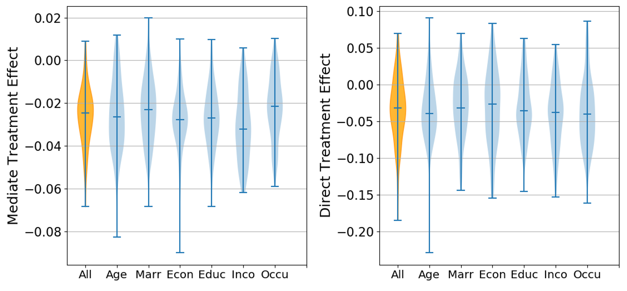
Figure 4: Our DTANet results on JobsII: The distributions of estimated treatment effect caused by different covariates for our DTANet.

7.4.2 Causal Explanations

The covariate/feature importance for the predictions is a simple but effective solution for explanations. Since our DTANet is causality-oriented, this experiment attempts to provide causal explanations for the estimated treatment effect by analyzing the contributions of input covariates.

Table 3: The distance (unit is $10^{-3}$) between the distribution of Mediate Treatment Effect / Direct Treatment Effect (using entire covariates) and that of excluding particular covariate.

	Age	Marr	Econ	Educ	Inco	Occu
Mediate	3.98	4.09	5.75	1.97	2.09	3.12
Direct	10.4	9.03	9.98	5.62	7.13	6.11

To accurately quantify the covariates importance, we repeatedly run our DTANet on JobsII and predict the treatment effect with different input covariates. We run DTANet on JobsII 100 trials, so we get 100 results and then obtain their distributions. As shown in Figure 4, $y$-axis is Mediate/Direct Treatment Effect and $x$-axis is the specific covariate excluded from entire covariates. The batch results colored in orange are gained by inputting all covariates. Each batch in blue corresponds to the estimated treatment effect by DTANet without a specific covariate. The estimated Mediate Treatment Effect is significantly different from zero, suggesting that treatment (job training) changes the mediate variable (job-search self-efficacy), which in turn changes the outcome (depressive symptoms). We find that three covariants, Econ (economic hardship), Marr (marital status) and Age, are the main causes of the treatment effect, which is consistent with study vinokur1997mastery . Particularly, we consider the distribution of Mediate/Direct Treatment Effect produced by entire covariates as the baselines. As shown in Figure 4, the distributions of excluding Econ, Marr and Age, respectively, are the three most significant ones that extend the baseline distribution with larger ranges. To further quantify the differences between baseline distributions and the distributions of excluding covariates, we resort to the original Wasserstein distance peyre2019computational as a metric in Table 3. Particularly, we use the function wasserstein_distance in python library SciPy to compute the Wasserstein distance between two distributions. For example, $3.98\times 10^{-3}$ is the Wasserstein distance between the distribution of Mediate Treatment Effect with entire covariates and the distribution excluding covariate Age. According to the results in Table 3, the distributions of Econ, Marr and Age have larger Wasserstein distances from the baseline distributions. In other words, these three covariates can significantly impact the Mediate/Direct Treatment Effect. This conclusion validates that the mediate feature representation in our DTANet method can generate effective causal explanations for the Mediate Treatment Effect estimation. On the other hand, the covariates contribute similar amounts to Direct Treatment Effect except Age. We can deduce that Age is the common cause for the treatment (job training) and outcome (depressive symptoms), i.e., the confounder.

Figure 5 demonstrates the estimated treatment effect when intervening on the mediator job search self-efficacy. The left figure shows magnitude of the estimated Mediate Treatment Effect increases slightly as one moves from lower to higher intervention factor. But the change is small, indicating the Mediate Treatment Effect is relatively constant across the distribution. In contrast, the estimated direct effects vary substantially across different intervention factors, although the confidence intervals are wide and always include zero.

7.4.3 Robustness analysis

There may exist unobserved confounders that causally affect both the mediator and outcome even after conditioning on the observed treatment and pre-treatment covariates. Therefore, we investigate the robustness of our DTANet to unmeasured confounding factor $\rho$. The robustness analysis is conducted by varying the value of $\rho$ and examining how the estimated treatment effect changes. We define $\rho$ as the correlation between the error terms in the mediator and the outcome models. This is reasonable, since unobserved confounder can bias both estimation of mediator and outcome, which further leads to unexplained variance or errors. If unobserved confounder affects mediator and outcome, we expect $\rho$ is non-zero.

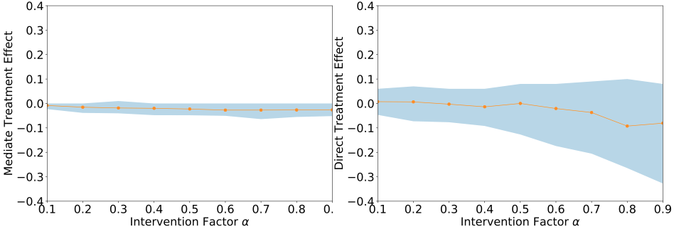
Figure 5: Our DTANet results on JobsII: the comparison of changes in estimated treatment effects caused by doing an intervention on the mediate variable. The blue cover represents 95% confidence interval of the change.

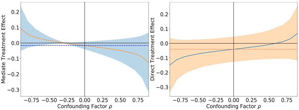
Figure 6: Robustness analysis of our DTANet on unobserved confounder. The dashed line represents the estimated mediation treatment effect. The areas represent 95% confidence interval for Mediate Treatment Effect at each $\rho$. The solid line represents the estimated average mediation effect at different values of $\rho$.

The estimates with potential outcome framework in Section 2.2 are identified if the ignorability assumption holds. However, it is possible that this assumption doesn’t holds in practice. Thus, we next ask how sensitive these estimates are to violations of this assumption using our method. Figure 6 shows the estimated mediator treatment effect and Direct Treatment Effect against different values of $\rho$, where $y$-axis is the treatment effect and $x$-axis is the confounding factor. The true Mediate Treatment Effect and Direct Treatment Effect marked as dash horizontal lines are -0.16 and -0.04, respectively. That means no unobserved confounders exists for mediator and outcomes (i.e., $\rho=0$). The left figure shows the confidence intervals for Mediate Treatment Effect (i.e., treatment effect due to mediation variable) covers the value of zero only under $\rho=-0.3$. The Mediate Treatment Effect is statistically indistinguishable from zero at the 95% level when the parameter $\rho<-0.3$. Potentially, parameter $\rho$ should be higher than $0.3$ so that the effect will be insignificant in the left figure, however such low $\rho$ value is unlikely to happen in practice. In other words, treatment effect estimation by our DTANet is robust to possible unobserved confounders in varying degrees.

8 Conclusion

Individual treatment effect (ITE) estimation is one major goal of causal inference, which aims to reduce the treatment assignment bias caused by the confounders. Although recent representation based methods achieve satisfactory computational accuracy, they overlook the unique characteristics of the treatment under different $do$ interventions. Moreover, the confounding representation from original covariates is easily affected by the treatment, which violates the fact that confounder is irrelevant to treatment after $do$ intervention. In order to overcome above challenges in individual treatment estimation (ITE), we propose an end-to-end model DTANet to learn the confounding representation by optimal transport, and it satisfies the treatment-invariant property introduced by doing an intervention. Meanwhile, by the proposed orthogonal projection strategy, DTANet is capable of capturing the mediate features that are treatment-specific and are informative for the outcome prediction. The effectiveness of DTANet is verified by both empirical and theoretical results.

References

- (1) Alaa, A.M., van der Schaar, M.: Bayesian inference of individualized treatment effects using multi-task gaussian processes. In: Advances in Neural Information Processing Systems, pp. 3424–3432 (2017)
- (2) Austin, P.C.: An introduction to propensity score methods for reducing the effects of confounding in observational studies. Multivariate behavioral research 46(3), 399–424 (2011)
- (3) Bang, H., Robins, J.M.: Doubly robust estimation in missing data and causal inference models. Biometrics 61(4), 962–973 (2005)
- (4) Benamou, J.D., Carlier, G., Cuturi, M., Nenna, L., Peyré, G.: Iterative bregman projections for regularized transportation problems. SIAM Journal on Scientific Computing 37(2), A1111–A1138 (2015)
- (5) Bottou, L., Peters, J., Quiñonero-Candela, J., Charles, D.X., Chickering, D.M., Portugaly, E., Ray, D., Simard, P., Snelson, E.: Counterfactual reasoning and learning systems: The example of computational advertising. The Journal of Machine Learning Research 14(1), 3207–3260 (2013)
- (6) Colnet, B., Mayer, I., Chen, G., Dieng, A., Li, R., Varoquaux, G., Vert, J.P., Josse, J., Yang, S.: Causal inference methods for combining randomized trials and observational studies: a review. arXiv preprint arXiv:2011.08047 (2020)
- (7) Concato, J., Shah, N., Horwitz, R.I.: Randomized, controlled trials, observational studies, and the hierarchy of research designs. New England journal of medicine 342(25), 1887–1892 (2000)
- (8) Courty, N., Flamary, R., Tuia, D.: Domain adaptation with regularized optimal transport. In: Joint European Conference on Machine Learning and Knowledge Discovery in Databases, pp. 274–289. Springer (2014)
- (9) Cuturi, M., Doucet, A.: Fast computation of wasserstein barycenters. In: International Conference on Machine Learning, pp. 685–693 (2014)
- (10) Davies, G.E., Soundy, T.J.: The genetics of smoking and nicotine addiction. South Dakota Medicine (2009)
- (11) Diamond, A., Sekhon, J.S.: Genetic matching for estimating causal effects: A general multivariate matching method for achieving balance in observational studies. Review of Economics and Statistics 95(3), 932–945 (2013)
- (12) Dudík, M., Langford, J., Li, L.: Doubly robust policy evaluation and learning. arXiv preprint arXiv:1103.4601 (2011)
- (13) Dung Duong, T., Li, Q., Xu, G.: Stochastic intervention for causal inference via reinforcement learning. arXiv e-prints pp. arXiv–2105 (2021)
- (14) Esfahani, P.M., Kuhn, D.: Data-driven distributionally robust optimization using the wasserstein metric: Performance guarantees and tractable reformulations. Mathematical Programming 171(1), 115–166 (2018)
- (15) Goldberger, A.S., et al.: Econometric theory. Econometric theory. (1964)
- (16) Hill, J.L.: Bayesian nonparametric modeling for causal inference. Journal of Computational and Graphical Statistics 20(1), 217–240 (2011)
- (17) Imbens, G.W.: The role of the propensity score in estimating dose-response functions. Biometrika 87(3), 706–710 (2000)
- (18) Johansson, F., Shalit, U., Sontag, D.: Learning representations for counterfactual inference. In: International conference on machine learning, pp. 3020–3029 (2016)
- (19) Johansson, F.D., Kallus, N., Shalit, U., Sontag, D.: Learning weighted representations for generalization across designs. arXiv preprint arXiv:1802.08598 (2018)
- (20) Kallus, N., Mao, X., Udell, M.: Causal inference with noisy and missing covariates via matrix factorization. arXiv preprint arXiv:1806.00811 (2018)
- (21) Kingma, D.P., Ba, J.: Adam: A method for stochastic optimization. arXiv preprint arXiv:1412.6980 (2014)
- (22) Kuroki, M., Pearl, J.: Measurement bias and effect restoration in causal inference. Biometrika 101(2), 423–437 (2014)
- (23) Lechner, M.: Identification and estimation of causal effects of multiple treatments under the conditional independence assumption. In: Econometric evaluation of labour market policies, pp. 43–58. Springer (2001)
- (24) Li, Q., Duong, T.D., Wang, Z., Liu, S., Wang, D., Xu, G.: Causal-aware generative imputation for automated underwriting. In: Proceedings of the 30th ACM International Conference on Information & Knowledge Management, pp. 3916–3924 (2021)
- (25) Li, Q., Niu, W., Li, G., Cao, Y., Tan, J., Guo, L.: Lingo: linearized grassmannian optimization for nuclear norm minimization. In: Proceedings of the 24th ACM International on Conference on Information and Knowledge Management, pp. 801–809 (2015)
- (26) Li, Q., Wang, X., Xu, G.: Be causal: De-biasing social network confounding in recommendation. arXiv preprint arXiv:2105.07775 (2021)
- (27) Li, Q., Wang, Z., Li, G., Pang, J., Xu, G.: Hilbert sinkhorn divergence for optimal transport. In: Proceedings of the IEEE/CVF Conference on Computer Vision and Pattern Recognition, pp. 3835–3844 (2021)
- (28) Li, Q., Wang, Z., Liu, S., Li, G., Xu, G.: Causal optimal transport for treatment effect estimation. IEEE transactions on neural networks and learning systems (2021)
- (29) Louizos, C., Shalit, U., Mooij, J.M., Sontag, D., Zemel, R., Welling, M.: Causal effect inference with deep latent-variable models. In: Advances in Neural Information Processing Systems, pp. 6446–6456 (2017)
- (30) Nichols, A.: Causal inference with observational data. The Stata Journal 7(4), 507–541 (2007)
- (31) Pearl, J.: Causal inference in statistics: An overview. Statistics surveys 3, 96–146 (2009)
- (32) Pearl, J.: Causality. Cambridge university press (2009)
- (33) Pearl, J., Glymour, M., Jewell, N.P.: Causal inference in statistics: A primer. John Wiley & Sons (2016)
- (34) Peyré, G., Cuturi, M., et al.: Computational optimal transport. Foundations and Trends in Machine Learning 11(5-6), 355–607 (2019)
- (35) Rosenbaum, P.R.: Observational study. Encyclopedia of statistics in behavioral science (2005)
- (36) Rosenbaum, P.R., Rubin, D.B.: The central role of the propensity score in observational studies for causal effects. Biometrika 70(1), 41–55 (1983)
- (37) Rubin, D.B.: Matching to remove bias in observational studies. Biometrics pp. 159–183 (1973)
- (38) Schnabel, T., Swaminathan, A., Singh, A., Chandak, N., Joachims, T.: Recommendations as treatments: Debiasing learning and evaluation. arXiv preprint arXiv:1602.05352 (2016)
- (39) Schwab, P., Linhardt, L., Karlen, W.: Perfect match: A simple method for learning representations for counterfactual inference with neural networks. arXiv preprint arXiv:1810.00656 (2018)
- (40) Shalit, U., Johansson, F.D., Sontag, D.: Estimating individual treatment effect: generalization bounds and algorithms. In: Proceedings of the 34th International Conference on Machine Learning-Volume 70, pp. 3076–3085. JMLR. org (2017)
- (41) Sun, W., Wang, P., Yin, D., Yang, J., Chang, Y.: Causal inference via sparse additive models with application to online advertising. In: Twenty-Ninth AAAI Conference on Artificial Intelligence (2015)
- (42) Villani, C.: Optimal transport: old and new, vol. 338. Springer Science & Business Media (2008)
- (43) Vinokur, A.D., Schul, Y.: Mastery and inoculation against setbacks as active ingredients in the jobs intervention for the unemployed. Journal of consulting and clinical psychology 65(5), 867 (1997)
- (44) Wager, S., Athey, S.: Estimation and inference of heterogeneous treatment effects using random forests. Journal of the American Statistical Association 113(523), 1228–1242 (2018)
- (45) Wang, Z., Li, Q., Li, G., Xu, G.: Polynomial representation for persistence diagram. In: Proceedings of the IEEE/CVF Conference on Computer Vision and Pattern Recognition, pp. 6123–6132 (2019)
- (46) Xu, G., Duong, T.D., Li, Q., Liu, S., Wang, X.: Causality learning: A new perspective for interpretable machine learning. arXiv preprint arXiv:2006.16789 (2020)