Lindbladian dynamics of the Sachdev-Ye-Kitaev model

Abstract

We study the Lindbladian dynamics of the Sachdev-Ye-Kitaev (SYK) model, where the SYK model is coupled to Markovian reservoirs with jump operators that are either linear or quadratic in the Majorana fermion operators. Here, the linear jump operators are non-random while the quadratic jump operators are sampled from a Gaussian distribution. In the limit of large $N$, where $N$ is the number of Majorana fermion operators, and also in the limit of large $N$ and $M$, where $M$ is the number of jump operators, the SYK Lindbladians are analytically tractable, and we obtain their stationary Green’s functions, from which we can read off the decay rate. For finite $N$, we also study the distribution of the eigenvalues of the SYK Lindbladians.

I Introduction

While quantum dynamics is often modeled by an idealized unitary time evolution, non-unitary time evolutions are ubiquitous and relevant since experimental systems are never completely isolated. Non-unitarity may arise in many different forms, such as dissipation, gain/loss, decoherence, measurements, and so on. Understanding and controlling these effects are of both fundamental and practical importance. Furthermore, non-unitarity may give rise to rich behaviors that do not have counterparts in systems governed by unitary time evolution. Our understanding of possible universal behaviors in open quantum systems, however, is still limited, particularly in the context of many-body quantum systems and quantum field theory.

In this paper, we study tractable many-body quantum systems with Lindbladian dynamics, aiming to deepen our understanding of open many-body quantum systems. The models we study consist of the SYK Hamiltonian, i.e., fermionic quantum many-body Hamiltonian with all-to-all interactions [1, 2] and jump operators that we will describe momentarily. Specifically, we consider a set of Majorana fermion operators, $\{\psi_{i},\psi_{j}\}=\delta_{ij}$, $\psi^{{\dagger}}_{i}=\psi_{i}$, and the associated Fock space where $i=1,\ldots,N$. The Lindbladian $\mathcal{L}$ of our interest, which generates the dynamics $d\rho/dt=\mathcal{L}(\rho)$, is given by

$$\mathcal{L}(\rho) =-i[H_{{\rm SYK}},\rho]+\sum_{\alpha}\left[L^{\ }_{\alpha}\rho L^{{\dagger}}_{\alpha}-\frac{1}{2}\{L^{{\dagger}}_{\alpha}L^{\ }_{\alpha},\rho\}\right].$$ (1)

Here, the Hamiltonian part is given by the SYK (SYK_q) Hamiltonian with $q$-body interaction,

$$H_{{\rm SYK}} =i^{q/2}\sum_{i_{1}<\cdots<i_{q}}J_{i_{1}\cdots i_{q}}\psi_{i_{1}}\cdots\psi_{i_{q}},$$ (2)

where $J_{i_{1}\cdots i_{q}}$ are random couplings drawn from the Gaussian distribution. As for the jump operators $\{L_{\alpha}\}$, we consider the following two cases. (i) First, we consider $N$ jump operators that are linear in fermion operators,

$$L^{i}=\sqrt{\mu}\psi^{i},\quad i=1,\cdots,N.$$ (3)

Here, $\mu$ is a nonrandom real parameter. (ii) In the second example, we consider $M$ quadratic jump operators,

$$L^{a} =\sum_{1\leq i<j\leq N}K^{a}_{ij}\psi_{i}\psi_{j},\quad K^{a}_{ij}\in\mathbb{C},\quad a=1,\cdots,M$$ (4)

where all $K^{a}_{ij}$ are independent complex Gaussian distributed random variables with mean and variance given by

$$\langle K^{a}_{ij}\rangle=0,\quad\langle|K^{a}_{ij}|^{2}\rangle=\frac{K^{2}}{N^{2}}\quad\forall\ i,j,a\quad\text{(no sum)}.$$ (5)

It is also possible to consider more generic jump operators that consist of $p$ Majorana operators. For more details on these models, see later sections. As we will show, these models can be analytically studied in the limit $N\to\infty$ in the first example, and in the limit $N,M\to\infty$, with fixed $R=M/N$, in the second example.

The SYK model and its variants have provided various tractable toy models for many-body problems, e.g., the butterfly effect, quantum information scrambling, quantum entanglement, non-Fermi liquids, etc., and have been extensively studied recently [3, 4, 5, 6, 7, 8, 9]. Some of these models admit holographic dual descriptions. We note that nonunitary time evolution of various kinds in SYK-type models has also been studied recently. See, for example, [10, 11, 12, 13, 14, 15, 16, 17, 18, 19, 20, 21]. Our study using the Lindbladian dynamics is different from and complementary to these previous works. The effects of dissipation in the SYK models have also been studied within unitary dynamics by including the heat bath degrees of freedom explicitly. There are two-coupled variants of SYK models, where one of the copies can be considered a bath. See, for example, [22, 23, 24]. At more technical levels, there are other Hermitian SYK type models (supersymmetric SYK and Wishert SYK models) that have some resemblance to our SYK Lindbladian model(s) [25, 26, 27].

In this work, we will study the properties of the above SYK Lindbladians by computing Green’s functions in the large-$N$ (and large-$M$) limit. This allows us to extract, for example, the dominant decay rate (the spectral gap of the Lindbladians). We also study spectral properties of finite-$N$ versions of the SYK Lindbladians by diagonalizing them numerically. The spectrum is complex in general and distributed non-trivially over the complex plane. Because of the all-to-all nature of interactions (and jump operators in the second case), the spectrum can be naturally compared with known behaviors in random Lindbladians studied by using techniques from Random Matrix Theory [28, 29, 30, 31, 32, 33, 34, 35, 36]. For the case of random quadratic jump operators, the spectrum crosses over from elliptic disk-shaped to “lemon-shaped” distribution by increasing the relative strength between the SYK interaction and the jump operators, $K/J$. The latter is a ubiquitous behavior in the strong dissipation regime of random Lindbladians [28, 29, 32]. We also observe clustering of eigenvalues by controlling the ratio $R=M/N$ [29, 30, 35].

II The operator-state isomorphism and the Schwinger-Keldysh path integral

We are interested in the spectral properties of the Lindbladians, and various correlation functions (mostly in the large-$N$ limit). To this end, we will set up a Schwinger-Keldysh type path-integral approach that involves two copies of path-integral variables [37, 38, 39]. We do so by first invoking the state-operator map (the Choi-Jamiołkowski isomorphism) to “vectorize” the Lindbladian. This allows us to think of operators (the density matrix in particular) as a state in the doubled Hilbert space, $\mathcal{H}\otimes\mathcal{H}^{*}\equiv\mathcal{H}_{+}\otimes\mathcal{H}_{-}$, and $\mathcal{L}$ as an operator acting on the doubled Hilbert space. The first step in the state-operator map is to consider a maximally entangled state $|\mathbb{I}\rangle$ in $\mathcal{H}_{+}\otimes\mathcal{H}_{-}$. This state should have a property that it maps or “reflects” all operators on the first Hilbert space to corresponding ones in the second Hilbert space (and vice versa): $O_{+}|\mathbb{I}\rangle=O^{\prime}_{-}|\mathbb{I}\rangle$, where $O_{+}$ and $O^{\prime}_{-}$ are some operators acting on the first and second Hilbert spaces. In particular, we require

$$\psi^{i}_{+}|\mathbb{I}\rangle=-i\psi^{i}_{-}|\mathbb{I}\rangle.$$ (6)

The factor of $-i$ originates from the Fermi statistics: reflecting twice gives a $2\pi$ rotation under which the fermion operators pick up $-1$. With $|\mathbb{I}\rangle$ in hand, we can map an operator, the density matrix $\rho$, say, to the corresponding state on $\mathcal{H}_{+}\otimes\mathcal{H}_{-}$ as

$$\rho\longrightarrow|\rho\rangle\equiv\rho_{+}|\mathbb{I}\rangle\in\mathcal{H}_{+}\otimes\mathcal{H}_{-}.$$ (7)

Note that the identity operator $\mathbb{I}$, which can be thought of as an infinite temperature Gibbs state, is mapped to $|\mathbb{I}\rangle$. Similarly, the Lindbladian can be mapped to an operator acting on $\mathcal{H}_{+}\otimes\mathcal{H}_{-}$, and the Lindblad equation is now written as $d|\rho\rangle/dt=\mathcal{L}|\rho\rangle$, where we continue to use $\mathcal{L}$ to represent the mapped operator. The explicit form of $\mathcal{L}$ for our models is given in equations (10) and (25). The state $\ket{\mathbb{I}}$ is annihilated by $\mathcal{L}$, $\mathcal{L}\ket{\mathbb{I}}=0$, as the infinite temperature state is stationary with respect to any Lindbladian.

With the operator-state map, for example, the “partition function” can be expressed as $\mathrm{Tr}\,[\rho(t)]=\langle\mathbb{I}|\rho(t)\rangle=\langle\mathbb{I}|e^{t\mathcal{L}}|\rho_{0}\rangle=\langle\mathbb{I}|\rho_{0}\rangle=1$ where $|\rho_{0}\rangle$ is an initial condition and we noted $\langle\mathbb{I}|e^{t\mathcal{L}}=\langle\mathbb{I}|$. Similarly, the expectation value of an operator $A$ is given by $\mathrm{Tr}\,[\rho(t)A]=\langle\mathbb{I}|A_{+}\otimes\mathbb{I}_{-}e^{t\mathcal{L}}|\rho_{0}\rangle$. These quantities can be readily expressed in terms of the coherent state path integral over two copies of real fermionic fields, $\psi^{i}_{\pm}(t)$, as

$$Z=\braket{\mathbb{I}}{e^{t\mathcal{L}}}{\rho_{0}}=\int\mathcal{D}\psi_{+}\mathcal{D}\psi_{-}e^{iS[\psi_{+},\psi_{-}]},$$ (8)

i.e., the Schwinger-Keldysh formalism.

For the SYK type models discussed below, we will analyze the Schwinger-Keldysh path integral (8) in the large-$N$ limit. Furthermore, in this work, we will be interested in stationary properties that may emerge in the late time limit. In particular, we will assume in this limit that the memory of the initial state is lost, and the system relaxes into a stationary state independent of the initial state.

III Non-random linear jump operators

In this section, we consider the SYK model in the presence of the jump operators

$$L^{i}=\sqrt{\mu}\psi^{i},\quad i=1,\cdots,N.$$ (9)

Here, we assume $\mu$ is a real parameter. Following the procedure outlined in the previous section, the Lindbladian acting on the doubled Hilbert space $\mathcal{H}_{+}\otimes\mathcal{H}_{-}$ is given by

$$\mathcal{L}=-iH_{{\rm SYK}}^{+}\otimes\mathbb{I}_{-}+i(-1)^{\frac{q}{2}}\mathbb{I}_{+}\otimes H_{{\rm SYK}}^{-}-i\mu\sum_{i}\psi_{+}^{i}\psi_{-}^{i}-\mu\frac{N}{2}\mathbb{I}_{+}\otimes\mathbb{I}_{-}.$$ (10)

At least superficially, this model looks similar to the two-coupled SYK model discussed in [22]. We however note various differences. The first is the relative phase between the $H_{{\rm SYK}}^{+}$ and $H_{{\rm SYK}}^{-}$ terms. For example, when $q=4$, we have opposite signs for these terms. The relative sign between the terms is necessary so that their sum is an isometry of $\ket{\mathbb{I}}$. On the other hand, for the regular two-coupled SYK model, these terms have the same sign, and induces time evolution. Another difference is that the Hamiltonian terms (the first two terms) are anti-Hermitian whereas $-i\mu\sum_{i}\psi_{+}^{i}\psi_{-}^{i}$ is Hermitian. Overall, $\mathcal{L}$ is not anti-Hermitian ($\mathcal{L}^{\dagger}\neq-\mathcal{L}$) and evolution is nonunitary.

III.1 Path integral and large-$N$ effective action

Using the formalism in the previous section, we can study this model using the Schwinger-Keldysh path integral. The action is given by

$$iS[\psi_{+},\psi_{-}] =\int_{t_{i}}^{t_{f}}dt\Bigg{[}-\frac{1}{2}\sum_{i}\psi^{i}_{+}\partial_{t}\psi^{i}_{+}-\frac{1}{2}\sum_{i}\psi^{i}_{-}\partial_{t}\psi^{i}_{-}-i^{q+1}\sum_{i_{1}<\cdots<i_{q}}J_{i_{1}\cdots i_{q}}\psi_{+}^{i_{1}}\cdots\psi_{+}^{i_{q}}$$

$$\qquad+i^{q+1}\sum_{i_{1}<\cdots<i_{q}}J_{i_{1}\cdots i_{q}}\psi_{-}^{i_{1}}\cdots\psi_{-}^{i_{q}}-i\mu\sum_{i}\psi_{+}^{i}(t)\psi_{-}^{i}(t)-\mu\frac{N}{2}\int dt1\Bigg{]}.$$ (11)

The action has to be supplemented with the proper boundary conditions at $t=t_{i},t_{f}$, set by the initial ($|\rho_{0}\rangle$) and final ($|\mathbb{I}\rangle$) states. When analyzing the stationary state, however, the boundary conditions are immaterial. This path integral can be studied in the large $N$ limit as in the regular SYK model. We introduce two kinds of matrix collective fields, $G_{\alpha\beta}(t_{1},t_{2})$ and $\Sigma_{\alpha\beta}(t_{1},t_{2})$, where $\alpha,\beta\in\{+,-\}$. The effective action for the collective fields is

$$S[G,\Sigma] =-\frac{iN}{2}\ln\det\,[-i(G_{0}^{-1}-\Sigma)]+\frac{i^{q+1}J^{2}N}{2q}\int_{t_{i}}^{t_{f}}dt_{1}dt_{2}\sum_{\alpha\beta}s_{\alpha\beta}G_{\alpha\beta}(t_{1},t_{2})^{q}$$

$$\qquad+\frac{iN}{2}\int_{t_{i}}^{t_{f}}dt_{1}dt_{2}\sum_{\alpha\beta}\Sigma_{\alpha\beta}(t_{1},t_{2})G_{\alpha\beta}(t_{1},t_{2})-i\frac{\mu N}{2}\int_{t_{i}}^{t_{f}}dt[G_{+-}(t,t)-G_{-+}(t,t)]+i\mu\frac{N}{2}\int dt,$$ (12)

where $s_{\alpha\beta}$ is given by

$$s_{++}=s_{--}=1,\qquad s_{+-}=s_{-+}=-(-1)^{\frac{q}{2}}.$$ (13)

In the saddle point approximation, the collective field $G_{\alpha\beta}$ is nothing but the Green’s functions of the fermion fields,

$$G_{\alpha\beta}(t_{1},t_{2})=-i\braket{T(\psi_{\alpha}(t_{1})\psi_{\beta}(t_{2}))}.$$ (14)

The correlation functions satisfy the symmetry relation $G_{\alpha\beta}(t_{1},t_{2})=-G_{\beta\alpha}(t_{2},t_{1})$. The partition function of the system in terms of the corrective fields is $Z=\int\mathcal{D}G_{\alpha\beta}\mathcal{D}\Sigma_{\alpha\beta}\exp\{iS[G,\Sigma]\}.$ The large $N$ saddle point equation is

$$i\partial_{t_{1}}G_{\alpha\beta}(t_{1},t_{2})-\int dt_{3}\sum_{\gamma=+,-}\Sigma_{\alpha\gamma}(t_{1},t_{3})G_{\gamma\beta}(t_{3},t_{2})=\delta_{\alpha\beta}\delta(t_{1}-t_{2}),$$ (15)

$$\Sigma_{\alpha\beta}(t_{1},t_{2})=-i^{q}J^{2}s_{\alpha\beta}G_{\alpha\beta}(t_{1},t_{2})^{q-1}+\mu\epsilon_{\alpha\beta}\delta(t_{1}-t_{2}).$$ (16)

III.2 Stationary Green’s functions

Large-$N$ limit with $q=4$

The saddle point equation can be analyzed numerically, or by taking the large $q$ limit. We first take $q=4$ and solve the Kadanoff-Baym equations (15) and (16) numerically. We note that assuming the memory of the initial state is lost in the long time limit, the time translation invariance is recovered and the collective fields depend only on $t_{1}-t_{2}\equiv t$. In Fig. 1, we show an example of the numerical stationary solution for $J=1$ and $\mu=0.250$. For large enough $\mu\gg J$, the system crosses over to the case of a dissipation-only model, where the correlation function decays exponentially with the decay rate given $\Gamma$ approaching $\mu$, as shown in Fig. 1. This is consistent with the spectrum at finite $N$, where an isolated cluster of eigenvalues forms at $-\mu$ when $\mu$ is large.

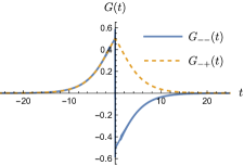
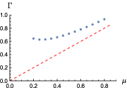
Figure 1: Top: The Green’s functions in the large-$N$ limit for $q=4$, $J=1$, and $\mu=0.250$. Bottom: The decay rate $\Gamma$ of the correlation functions as a function of $\mu$. For large $\mu/J$, the decay rate approaches $\Gamma=\mu$ (red dashed line).

Large-$q$ limit

In the large-$q$ limit, we expand the Green’s function as [4]

$$G_{\alpha\beta}(t_{1},t_{2}) =G^{0}_{\alpha\beta}(t_{1},t_{2})\Big{(}1+\frac{1}{q}g_{\alpha\beta}(t_{1},t_{2})+\cdots\Big{)},$$ (17)

The Kadanoff-Baym equation then reduces to the Liouville equation

$$\partial_{t_{1}}\partial_{t_{2}}g_{++}(t_{1},t_{2}) =-2\mathcal{J}^{2}e^{g_{++}(t_{1},t_{2})},$$

$$\partial_{t_{1}}\partial_{t_{2}}g_{+-}(t_{1},t_{2}) =-2\mathcal{J}^{2}e^{g_{+-}(t_{1},t_{2})}-2\hat{\mu}\delta(t_{1}-t_{2}).$$ (18)

Here we have defined $J^{2}=\frac{2^{q-1}\mathcal{J}^{2}}{q}$ and $\mu=\frac{\hat{\mu}}{q}$. We impose the boundary conditions as

$$g_{++}(t,t)=0,$$

$$\lim_{t_{2}\to t_{1}}\partial_{t_{1}}g_{+-}(t_{1},t_{2})=-\hat{\mu},$$

$$g_{++}(t_{1},t_{2})-g_{+-}(t_{1},t_{2})\to 0\text{ as }t_{1}\to\infty.$$ (19)

We can then obtain a stationary solution as

$$e^{g_{++}(t)}=\frac{\alpha^{2}}{\mathcal{J}^{2}\cosh^{2}(\alpha|t|+\gamma)},$$

$$e^{g_{+-}(t)}=\frac{\tilde{\alpha}^{2}}{\mathcal{J}^{2}\cosh^{2}(\tilde{\alpha}|t|+\tilde{\gamma})}.$$ (20)

To satisfy the boundary conditions, we impose

$$\frac{\alpha}{\mathcal{J}\cosh\gamma}=1,\quad\hat{\mu}=2\tilde{\alpha}\tanh\tilde{\gamma},\quad\alpha=\tilde{\alpha},\quad\gamma=\tilde{\gamma}.$$ (21)

By solving these conditions, we obtain

$$\alpha=\tilde{\alpha}=\mathcal{J}\sqrt{\Big{(}\frac{\hat{\mu}}{2\mathcal{J}}\Big{)}^{2}+1},\quad\gamma=\tilde{\gamma}=\text{arcsinh}\Big{(}\frac{\hat{\mu}}{2\mathcal{J}}\Big{)}.$$ (22)

From these, we see that the correlation functions behave as $G(t)\sim e^{\frac{g(t)}{q}}$ and decay exponentially. We can read off $\frac{2\alpha}{q}\equiv\Gamma$ as the decay rate. This behavior also qualitatively agrees with the $\mu$ dependence for the $q=4$ case above analyzed numerically. Also, for large $q$, we can confirm that as $\mu\to 0$ (after taking the long-time limit), the Green’s function reduces to the infinite temperature thermal Green’s function.

III.3 Finite $N$ spectrum

We now turn to the spectral properties of the SYK Lindbladian (10). The complex spectrum $\{\lambda_{i}\}$ of the SYK Lindbladian (10) can be studied by numerical exact diagonalization for finite $N$. We set $N=8$ in our analysis below, which means, including both copies $\psi^{i}_{+}$ and $\psi^{i}_{-}$, we have $2N=16$ flavors of Majorana fermion operators. Plotted in Fig. 2 are the numerical spectra $\{\lambda_{i}\}$ for representative choices of $\mu$ (we set $J=1$). For each $\mu$, $100$ disorder realizations were collected.

For small $\mu$, there are many eigenvalues centered around $\text{Re}\,(\lambda)=-N\mu/2$. As we increase $\mu$, vertical bands of eigenvalues start forming along the real axis. Each band is located roughly along a line ${\rm Re}\,(\lambda)=-\mu n$ for $n=1,\ldots,N$. As we increase $\mu$ even further, all the eigenvalues become close to real. This reminds us of a real-complex transition in some non-Hermitian systems [40]. Another effect of increasing $\mu$ is the formation of clusters around $\lambda=-n\mu$, with gaps in between. The cluster formation first occurs at the left and right edges of the spectrum, i.e. at small and large $n$, and then subsequently occurs at intermediate values of $n$. Similar band and cluster formation and hierarchy of relaxation times were observed in Refs. [30, 35], although we should note that these works studied purely dissipative random Lindbladians, while in our model the randomness enters only in the Hamiltonian part.

In the weak dissipation regime, that is $\mu/J<0.5$, the non-linearity in the decay rate and the band-formation in the spectrum indicates that there is a non-trivial competition between the dissipative and SYK interactions.

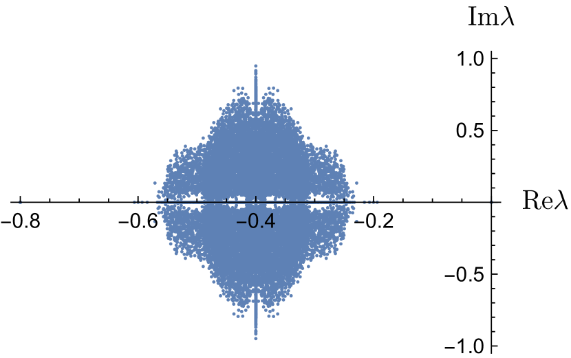
(a) $\mu=0.1$

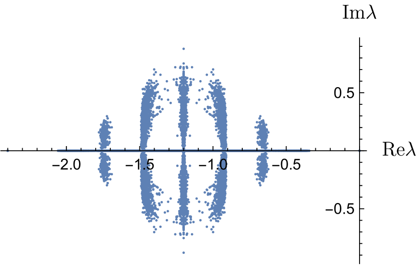
(b) $\mu=0.3$

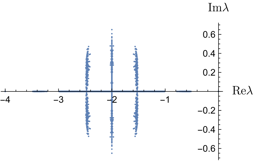
(c) $\mu=0.5$

(d) $\mu=0.9$

Figure 2: Spectrum of the SYK Lindbladian operator $\mathcal{L}$ (10) for $\mu=0.1,0.3,0.5$ and $0.9$ with $J=1$.

IV Random quadratic jump operators

In this section we consider another open SYK system. Here we introduce $M$ two-body jump operators $L^{a}$ with random couplings. The Hamiltonian and the jump operators respectively are:

$$\begin{split}H_{\text{SYK}}&=i^{q/2}\sum_{1\leq i_{1}<\cdots<i_{q}\leq N}J_{i_{1}\cdots i_{q}}\psi_{i_{1}}\cdots\psi_{i_{q}},\\ L^{a}&=\sum_{1\leq i<j\leq N}K^{a}_{ij}\psi_{i}\psi_{j},\quad K^{a}_{ij}\in\mathbb{C},\quad a=1,\cdots,M.\end{split}$$ (23)

All $K^{a}_{ij}$ are independent identically distributed complex Gaussian random variables with mean and variance given by

$$\langle{K^{a}_{ij}}\rangle=0,\quad\langle{|K^{a}_{ij}|^{2}}\rangle=\frac{K^{2}}{N^{2}}\quad\forall i,j,a\quad\text{(no sum)}.$$ (24)

The Lindbladian acting on the doubled Hilbert space $\mathcal{H}_{+}\otimes\mathcal{H}_{-}$ is given by

$$\begin{split}\mathcal{L}&=-iH_{{\rm SYK}}^{+}\otimes\mathbb{I}_{-}+i(-1)^{\frac{q}{2}}\mathbb{I}_{+}\otimes H_{{\rm SYK}}^{-}-\sum_{a}L_{+}^{a}\otimes L^{a}_{-}{}^{\dagger}-\frac{1}{2}\sum_{a}L^{a}_{+}{}^{\dagger}L^{a}_{+}\otimes\mathbb{I}_{-}-\frac{1}{2}\mathbb{I}_{+}\otimes\sum_{a}L^{a}_{-}L^{a}_{-}{}^{\dagger}\\ &=-iH_{{\rm SYK}}^{+}\otimes\mathbb{I}_{-}+i(-1)^{\frac{q}{2}}\mathbb{I}_{+}\otimes H_{{\rm SYK}}^{-}+\sum_{a}\sum_{i<j}\sum_{k<l}K^{a}_{ij}\bar{K}^{a}_{kl}\left(\psi^{i}_{+}\psi^{j}_{+}\psi^{k}_{-}\psi^{l}_{-}+\frac{1}{2}\psi^{k}_{+}\psi^{l}_{+}\psi^{i}_{+}\psi^{j}_{+}+\frac{1}{2}\psi^{i}_{-}\psi^{j}_{-}\psi^{k}_{-}\psi^{l}_{-}\right).\end{split}$$ (25)

IV.1 Path integral and large-$N$ effective action

Using the formalism in Section II, we can obtain the Schwinger-Keldysh action for this model. Since we will be analyzing the stationary state, the initial state $\ket{\rho_{0}}$ is immaterial, and will be excluded from the path integral. We introduce complex Hubbard-Stratonovich (or auxiliary) fields $b^{a}_{+}(t)$ and $\ b^{a}_{-}(t)$ to make the dissipation term linear with respect to the jump operators. The resulting action is as follows:

$$\begin{split}&iS[\psi_{+},\psi_{-},b^{a}_{+},b^{a}_{-},\bar{b}^{a}_{+},\bar{b}^{a}_{-}]\\ =&\int dt\Bigg{[}-\frac{1}{2}\sum_{i}\psi^{i}_{+}\partial_{t}\psi^{i}_{+}-\frac{1}{2}\sum_{i}\psi^{i}_{-}\partial_{t}\psi^{i}_{-}-i^{q/2+1}\sum_{i_{1}<\cdots<i_{q}}J_{i_{1}\cdots i_{q}}\psi_{+}^{i_{1}}\cdots\psi_{+}^{i_{q}}-(-i)^{q/2+1}\sum_{i_{1}<\cdots<i_{q}}J_{i_{1}\cdots i_{q}}\psi_{-}^{i_{1}}\cdots\psi_{-}^{i_{q}}\\ &\qquad\qquad-\frac{1}{2}\sum_{a}\begin{pmatrix}\bar{b}^{a}_{+}(t)&\bar{b}^{a}_{-}(t)\end{pmatrix}\begin{pmatrix}1&0\\ -2&1\end{pmatrix}\begin{pmatrix}b^{a}_{+}(t)\\ b^{a}_{-}(t)\end{pmatrix}\\ &\qquad\qquad+\frac{1}{2}\sum_{a}\left(\bar{b}^{a}_{+}(t)L^{a}_{+}(t)+\bar{b}^{a}_{-}(t)L^{a}_{-}(t)+b^{a}_{+}(t)\bar{L}^{a}_{+}(t)+b^{a}_{-}(t)\bar{L}^{a}_{-}(t)\right)\Bigg{]}.\end{split}$$ (26)

We then perform disorder averaging over the random couplings $J$ and $K$. Next, we introduce collective fields for both, the fermion fields and the auxiliary fields. We denote the fermion collective fields by $G_{\alpha\beta}$ and $\Sigma_{\alpha\beta}$, and the auxiliary collective fields by $G^{b}_{\alpha\beta}$ and $\Sigma^{b}_{\alpha\beta}$, where $\alpha,\beta=\pm$. Consider the limit $N,M\rightarrow\infty$ with constant $R=M/N$. In this limit, the Green’s functions and self energies of the system are determined by the saddle point of the action. The saddle point equations are as follows:

$$\begin{split}\Sigma^{b}_{\alpha\beta}(t_{1},t_{2})=&\frac{K^{2}}{4}G_{\alpha\beta}(t_{1},t_{2})^{2},\\ \mathbf{G}^{b}(t_{1},t_{2})=&\left[\begin{pmatrix}1&0\\ -2&1\end{pmatrix}\delta(t_{1}-t_{2})-\mathbf{\Sigma}^{b}(t_{1},t_{2})\right]^{-1},\\ \Sigma_{\alpha\beta}(t_{1},t_{2})=&-i^{q}J^{2}s_{\alpha\beta}G_{\alpha\beta}(t_{1},t_{2})^{q-1}+\frac{K^{2}R}{2}\left(G^{b}_{\alpha\beta}(t_{1},t_{2})+G^{b}_{\beta\alpha}(t_{2},t_{1})\right)G_{\alpha\beta}(t_{1},t_{2}),\\ \mathbf{G}(t_{1},t_{2})=&\left[\mathbf{G}_{0}^{-1}(t_{1},t_{2})-\mathbf{\Sigma}(t_{1},t_{2})\right]^{-1}.\end{split}$$ (27)

The boldface fields are $2\times 2$ matrices with $\pm$ indices. The matrix inverses are with respect to this $2\times 2$ matrix multiplication as well as the time domain multiplication. Now let us apply the stationary state hypothesis to obtain the Schwinger-Dyson equations:

$$\begin{split}\Sigma^{b}_{\alpha\beta}(t)=&\frac{K^{2}}{4}G_{\alpha\beta}(t)^{2},\\ \mathbf{G}^{b}(\omega)=&\left(\begin{pmatrix}1&0\\ -2&1\end{pmatrix}-\mathbf{\Sigma}^{b}(\omega)\right)^{-1},\\ \Sigma_{\alpha\beta}(t)=&-i^{q}J^{2}s_{\alpha\beta}G_{\alpha\beta}(t)^{q-1}+\frac{K^{2}R}{2}\left(G^{b}_{\alpha\beta}(t)+G^{b}_{\beta\alpha}(-t)\right)G_{\alpha\beta}(t),\\ \mathbf{G}(\omega)=&(\mathbf{G}_{0}^{-1}(\omega)-\mathbf{\Sigma}(\omega))^{-1}.\end{split}$$ (28)

IV.2 Stationary Green’s functions

We solve (28) numerically for $q=4$ and various values of the parameters $J,K,$ and $R$. For all these solutions, the Green’s functions of the Hubbard-Stratanovich fields are numerically consistent with the following trivial solution:

$$\mathbf{G}^{b}(t)=\begin{pmatrix}1&0\\ 2&1\end{pmatrix}\delta(t).$$

In all cases, the fermion Green’s functions decay exponentially at late times. For small dissipation strength, the Green’s functions oscillate as they decay. To characterize these oscillation we try to fit the retarded Green’s function $G^{R}(t)=-i\Theta(t)[G_{+-}(t)-G_{-+}(t)]$ with the following ansatz at late times.

$$G^{R}(t)\approx Ae^{-\Gamma t}\sin(\omega_{0}t+\phi).$$ (29)

Figure 3 shows the late time decay rate $\Gamma$ and frequency $\omega_{0}$ of the retarded Green’s function, obtained by fitting this ansatz to the numerical solutions. Here we have fixed $J=1$ and $R=2$. As the dissipation strength $K$ is increased, we see a transition from damped oscillations $(\omega_{0}>0)$ to a purely exponential decay $(\omega_{0}=0)$ of $G^{R}(t)$ at around $K\sim 0.4$. This is analogous to the transition observed in the Caldeira-Leggett model, a canonical example of open quantum dynamics [41]. The decay rate $\Gamma$ is expected to increases with stronger dissipation. While this is generally true, in a small window right after the transition, the decay rate decreases as dissipation becomes stronger. This can be interpreted as the quantum Zeno effect in which, frequent measurement or strong environmental coupling (as in this case) can stabilize a quantum state [42, 43, 44, 45].

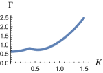
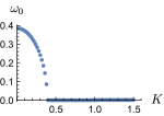
Figure 3: Decay rate $\Gamma$ and frequency $\omega_{0}$ of late time $G^{R}(t)$ for $J=1,R=2$.

In the frequency domain, a useful quantity to analyze is the spectral function defined by

$$A(\omega)=-2\ \text{Im}\,[G^{R}(\omega)].$$ (30)

The spectral function can be interpreted as a probability distribution. Indeed, our numerical solutions satisfy the normalization condition $\int_{-\infty}^{\infty}\frac{d\omega}{2\pi}A(\omega)=1$. We compare the spectral function to a Lorentzian distribution. Figure 4 demonstrates that for large dissipation strength $K$, $A(\omega)$ is well approximated by a Lorentzian. We see the same effect at large $R$, that is, for a large number of jump operators. The Lehman representation for Lindbladian systems [46] suggests that when the spectral function is Lorentzian the eigenvalue with the largest non-zero real part is purely real. This is consistent with our finite $N$ numerics in the next section.

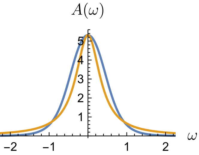
(a) $K=0.1$

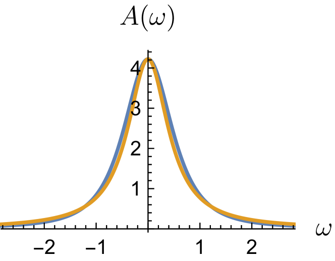
(b) $K=0.5$

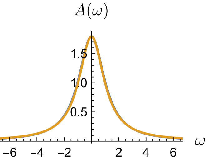
(c) $K=1$

Figure 4: Spectral function (blue) compared with Lorentzian (orange) for $J=1,R=2$.

IV.3 Finite $N$ spectrum

The stationary Green’s functions naturally do not contain all the information about the dynamics of the system. The full information of the dynamics is contained in the eigenvalues and eigenvectors of the Lindbladian [47]. Here, we will study the eigenvalues, also known as the spectrum, of the Lindbladian (23). We set $N=10$, which gives a total of $20$ Majorana fields after the doubling described in Section II. For each set of parameters, we collect 50 realizations of the random Lindbladian to plot the spectrum.

Figure 5 shows the spectra as we vary $K$ while keeping $J=1$ and $R=1$ fixed. For large dissipation strength $K$, the boundary of the spectrum resembles a lemon-shape. We compare this boundary to the spectral boundary of purely disipative fully random Lindblad operators, which was calculated analytically in [28]. To do this comparison, we first scale and shift the eigenvalues as follows:

$$\lambda_{i}\rightarrow\sqrt{N}\left(\frac{8}{NK^{2}}\lambda_{i}+1\right).$$ (31)

Note that the dissipative part of the Lindbladian in Equation (25) contains $\sim N^{2}$ random entries, whereas a fully random Lindbladian on the $2^{N/2}$-dimensional Hilbert space would contain $\sim 2^{N}$ random entries. Also, only two-body jump operators are considered in this model. Therefore, the boundary of the spectrum may not precisely match the contour derived in [28], and further investigation is required. When the dissipation strength $K$ is small relative to the SYK coupling $J$, the spectrum is elliptical. The spectra also show an enhanced density of eigenvalues on the real axis. These features resemble those of random Lindbladians reported in [28, 29, 32].

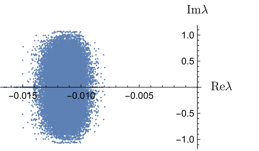
(a) $K=0.1$

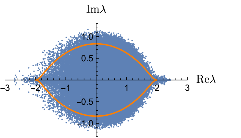
(b) $K=1.5$ (scaled)

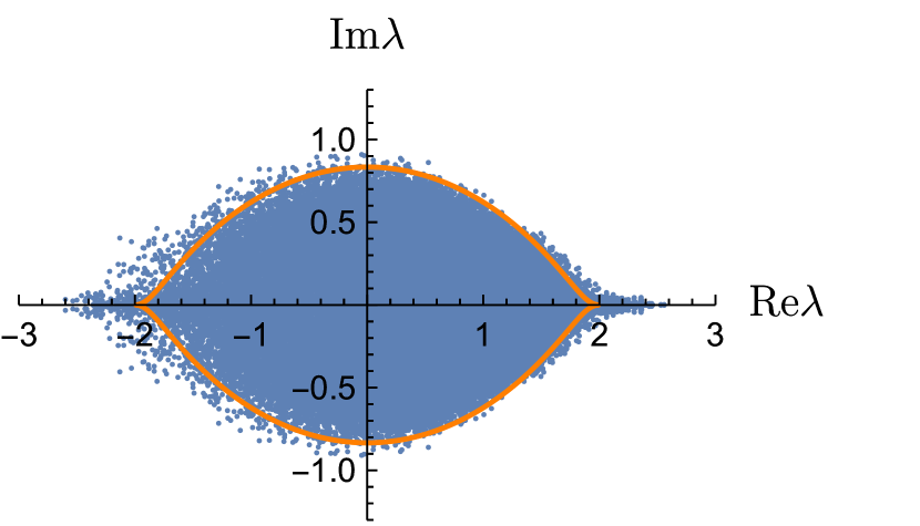
(c) $K=3$ (scaled)

Figure 5: Spectrum of the Lindbladian (25) for $J=1,R=1$ and varying $K$. (a) The spectrum is elliptical, consistent with the literature. (b) and (c) The spectrum is scaled and shifted according to equation (31) before being plotted. As $K$ increases, the boundary of this (scaled) spectrum resembles the lemon-shaped contour derived in [28].

The story is quite different when we vary $R$ while keeping $J$ and $K$ fixed. Figure 6 shows that the shape of the spectrum changes significantly as we increase $R$. The bulk of the spectrum gets progressively squeezed towards the negative real axis, while clusters of (close to) real eigenvalues are left in its wake. Similar cluster formation and hierarchy of relaxation times were observed in random Lindbladians [29, 30, 35].

In unitary physics, random matrix theory captures the universal features of chaotic dynamics. To understand whether this is also the case in nonunitary physics, it is important to identify physical systems that exhibit nonunitary random matrix behavior. As we have seen, the model (23) indeed serves this purpose.

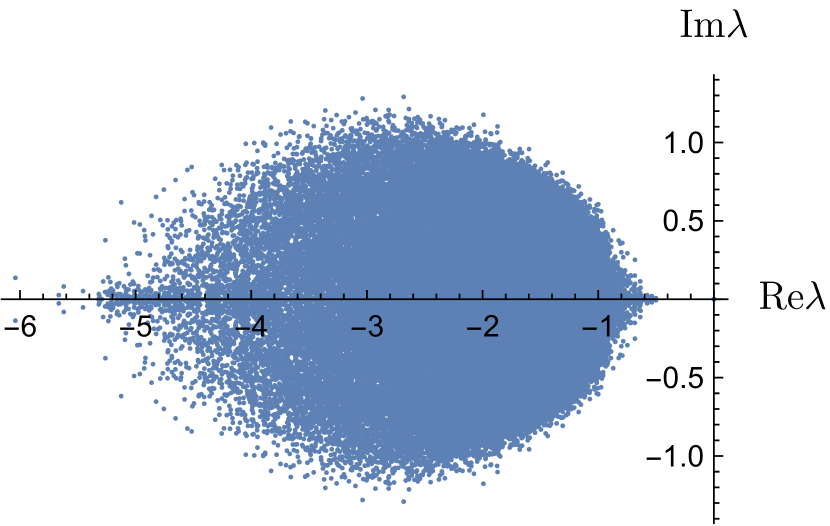
(a) $R=0.5$

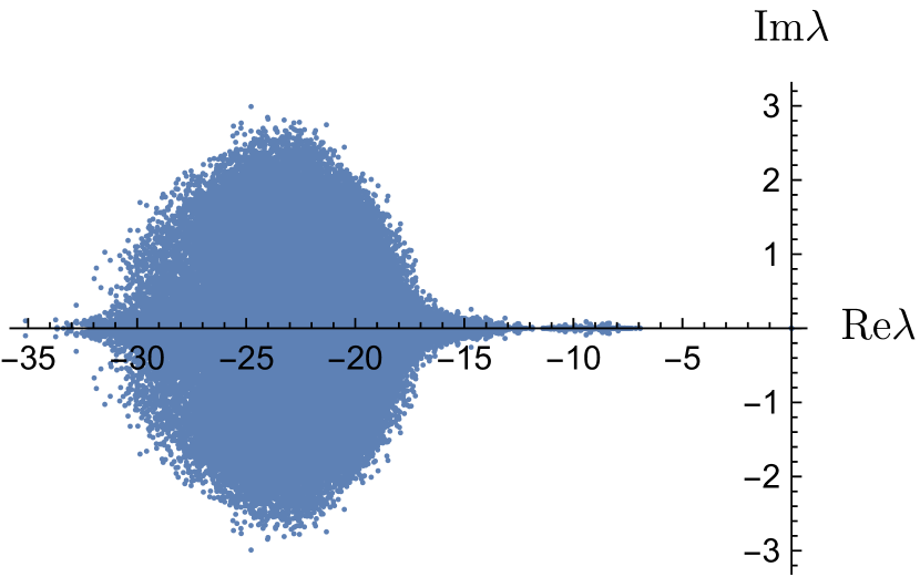
(b) $R=5$

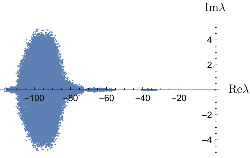
(c) $R=20$

Figure 6: Spectrum of the Lindbladian (25) for $J=1,K=2$ and varying $R$

V Summary and outlook

In this work, we introduced SYK type Lindbladian models and studied their Green’s functions in the long time limit, and their spectral properties. The models admit exact analysis in various limits (large $N$, large $q$, simultaneous large $N$ and $M$ limits). Another merit of the models is that they exhibit very rich behaviors. In particular, the second model realizes many different behaviors by simply controlling the parameters $J,K,$ and $R$, some of which compare well with different random Lindbladian models studied previously. There are many remaining questions. We close by listing a few of them. First, vast generalizations of the current models are possible, for example, by introducing $p$-body jump operators. Studying wider classes of models would allow us to explore different universal behaviors in open quantum many-body systems. Second, while we studied the distribution of the eigenvalues of the SYK Lindbladians, a more thorough characterization of the spectral properties is necessary. For example, it is of great interest to study the level statistics [34, 20, 48, 49]. The level statistics may show an interesting crossover as the distribution crosses over from the lemon shape to the one with many clusters [50]. Third, in this work, we mostly focused on stationary properties. However, it would be interesting to follow the time evolution by the SYK Lindbladians starting from some initial state. Technically, the Kadanoff-Baym equation can be solved numerically.

Note added: Recently, [51] appeared on arXiv, which has a substantial overlap with our Section IV.

References

- Sachdev and Ye [1993] S. Sachdev and J. Ye, Gapless spin-fluid ground state in a random quantum Heisenberg magnet, Phys. Rev. Lett. 70, 3339 (1993), arXiv:cond-mat/9212030 [cond-mat] .
- Kitaev [2015] A. Kitaev, A simple model of quantum holography, Talks at KITP (2015).
- Polchinski and Rosenhaus [2016] J. Polchinski and V. Rosenhaus, The Spectrum in the Sachdev-Ye-Kitaev Model, JHEP 04, 001, arXiv:1601.06768 [hep-th] .
- Maldacena and Stanford [2016] J. Maldacena and D. Stanford, Remarks on the Sachdev-Ye-Kitaev model, Phys. Rev. D 94, 106002 (2016), arXiv:1604.07818 [hep-th] .
- Gu et al. [2017] Y. Gu, X.-L. Qi, and D. Stanford, Local criticality, diffusion and chaos in generalized Sachdev-Ye-Kitaev models, JHEP 05, 125, arXiv:1609.07832 [hep-th] .
- Song et al. [2017] X.-Y. Song, C.-M. Jian, and L. Balents, Strongly Correlated Metal Built from Sachdev-Ye-Kitaev Models, Phys. Rev. Lett. 119, 216601 (2017), arXiv:1705.00117 [cond-mat.str-el] .
- Altland et al. [2019] A. Altland, D. Bagrets, and A. Kamenev, Quantum Criticality of Granular Sachdev-Ye-Kitaev Matter, Phys. Rev. Lett. 123, 106601 (2019), arXiv:1903.09491 [cond-mat.str-el] .
- Rosenhaus [2019] V. Rosenhaus, An introduction to the SYK model, Journal of Physics A Mathematical General 52, 323001 (2019), arXiv:1807.03334 [hep-th] .
- Chowdhury et al. [2021] D. Chowdhury, A. Georges, O. Parcollet, and S. Sachdev, Sachdev-Ye-Kitaev Models and Beyond: A Window into Non-Fermi Liquids, arXiv e-prints , arXiv:2109.05037 (2021), arXiv:2109.05037 [cond-mat.str-el] .
- Liu et al. [2020] C. Liu, P. Zhang, and X. Chen, Non-unitary dynamics of Sachdev-Ye-Kitaev chain, arXiv e-prints , arXiv:2008.11955 (2020), arXiv:2008.11955 [cond-mat.str-el] .
- García-García and Godet [2021] A. M. García-García and V. Godet, Euclidean wormhole in the Sachdev-Ye-Kitaev model, Phys. Rev. D 103, 046014 (2021), arXiv:2010.11633 [hep-th] .
- García-García et al. [2021a] A. M. García-García, Y. Jia, D. Rosa, and J. J. M. Verbaarschot, Replica Symmetry Breaking and Phase Transitions in a PT Symmetric Sachdev-Ye-Kitaev Model, arXiv e-prints , arXiv:2102.06630 (2021a), arXiv:2102.06630 [hep-th] .
- Zhang et al. [2021] P. Zhang, S.-K. Jian, C. Liu, and X. Chen, SYK Meets Non-Hermiticity I: Emergent Replica Conformal Symmetry, arXiv e-prints , arXiv:2104.04088 (2021), arXiv:2104.04088 [cond-mat.str-el] .
- Jian et al. [2021] S.-K. Jian, C. Liu, X. Chen, B. Swingle, and P. Zhang, SYK meets non-Hermiticity II: measurement-induced phase transition, arXiv e-prints , arXiv:2104.08270 (2021), arXiv:2104.08270 [cond-mat.str-el] .
- Jian and Swingle [2021] S.-K. Jian and B. Swingle, Phase transition in von Neumann entanglement entropy from replica symmetry breaking, arXiv e-prints , arXiv:2108.11973 (2021), arXiv:2108.11973 [quant-ph] .
- Cornelius et al. [2021] J. Cornelius, Z. Xu, A. Saxena, A. Chenu, and A. del Campo, Spectral Filtering Induced by Non-Hermitian Evolution with Balanced Gain and Loss: Enhancing Quantum Chaos, arXiv e-prints , arXiv:2108.06784 (2021), arXiv:2108.06784 [quant-ph] .
- Zanoci and Swingle [2021] C. Zanoci and B. Swingle, Energy Transport in Sachdev-Ye-Kitaev Networks Coupled to Thermal Baths, arXiv e-prints , arXiv:2109.03268 (2021), arXiv:2109.03268 [cond-mat.str-el] .
- Xu et al. [2021] Z. Xu, A. Chenu, T. Prosen, and A. del Campo, Thermofield dynamics: Quantum chaos versus decoherence, Phys. Rev. B 103, 064309 (2021), arXiv:2008.06444 [quant-ph] .
- Su et al. [2021] K. Su, P. Zhang, and H. Zhai, Page curve from non-Markovianity, Journal of High Energy Physics 2021, 156 (2021), arXiv:2101.11238 [cond-mat.str-el] .
- García-García et al. [2021b] A. M. García-García, L. Sá, and J. J. M. Verbaarschot, Symmetry classification and universality in non-Hermitian many-body quantum chaos by the Sachdev-Ye-Kitaev model, arXiv e-prints , arXiv:2110.03444 (2021b), arXiv:2110.03444 [hep-th] .
- Altland et al. [2021] A. Altland, M. Buchhold, S. Diehl, and T. Micklitz, Dynamics of measured many-body quantum chaotic systems, arXiv e-prints , arXiv:2112.08373 (2021), arXiv:2112.08373 [cond-mat.dis-nn] .
- Maldacena and Qi [2018] J. Maldacena and X.-L. Qi, Eternal traversable wormhole, arXiv e-prints , arXiv:1804.00491 (2018), arXiv:1804.00491 [hep-th] .
- Maldacena and Milekhin [2019] J. Maldacena and A. Milekhin, SYK wormhole formation in real time, arXiv e-prints , arXiv:1912.03276 (2019), arXiv:1912.03276 [hep-th] .
- Kim et al. [2019] J. Kim, I. R. Klebanov, G. Tarnopolsky, and W. Zhao, Symmetry Breaking in Coupled SYK or Tensor Models, Physical Review X 9, 021043 (2019), arXiv:1902.02287 [hep-th] .
- Fu et al. [2017] W. Fu, D. Gaiotto, J. Maldacena, and S. Sachdev, Publisher’s Note: Supersymmetric Sachdev-Ye-Kitaev models [Phys. Rev. D 95, 026009 (2017)], Phys. Rev. D 95, 069904 (2017), arXiv:1610.08917 [hep-th] .
- Bi et al. [2017] Z. Bi, C.-M. Jian, Y.-Z. You, K. A. Pawlak, and C. Xu, Instability of the non-Fermi-liquid state of the Sachdev-Ye-Kitaev model, Phys. Rev. B 95, 205105 (2017), arXiv:1701.07081 [cond-mat.str-el] .
- Sá and García-García [2021] L. Sá and A. M. García-García, The Wishart-Sachdev-Ye-Kitaev model: Q-Laguerre spectral density and quantum chaos, arXiv e-prints , arXiv:2104.07647 (2021), arXiv:2104.07647 [hep-th] .
- Denisov et al. [2019] S. Denisov, T. Laptyeva, W. Tarnowski, D. Chruściński, and K. Życzkowski, Universal Spectra of Random Lindblad Operators, Phys. Rev. Lett. 123, 140403 (2019), arXiv:1811.12282 [quant-ph] .
- Can et al. [2019] T. Can, V. Oganesyan, D. Orgad, and S. Gopalakrishnan, Spectral Gaps and Midgap States in Random Quantum Master Equations, Phys. Rev. Lett. 123, 234103 (2019), arXiv:1902.01414 [quant-ph] .
- Wang et al. [2020] K. Wang, F. Piazza, and D. J. Luitz, Hierarchy of Relaxation Timescales in Local Random Liouvillians, Phys. Rev. Lett. 124, 100604 (2020), arXiv:1911.05740 [cond-mat.str-el] .
- Can [2019] T. Can, Random Lindblad dynamics, Journal of Physics A Mathematical General 52, 485302 (2019), arXiv:1902.01442 [quant-ph] .
- Sá et al. [2020a] L. Sá, P. Ribeiro, and T. Prosen, Spectral and steady-state properties of random Liouvillians, Journal of Physics A Mathematical General 53, 305303 (2020a), arXiv:1905.02155 [quant-ph] .
- Sá et al. [2020b] L. Sá, P. Ribeiro, T. Can, and T. Prosen, Spectral transitions and universal steady states in random Kraus maps and circuits, Phys. Rev. B 102, 134310 (2020b), arXiv:2007.04326 [cond-mat.stat-mech] .
- Sá et al. [2020c] L. Sá, P. Ribeiro, and T. Prosen, Complex Spacing Ratios: A Signature of Dissipative Quantum Chaos, Physical Review X 10, 021019 (2020c), arXiv:1910.12784 [cond-mat.stat-mech] .
- Li et al. [2021] J. L. Li, D. C. Rose, J. P. Garrahan, and D. J. Luitz, Random matrix theory for quantum and classical metastability in local Liouvillians, arXiv e-prints , arXiv:2110.13158 (2021), arXiv:2110.13158 [cond-mat.str-el] .
- Tarnowski et al. [2021] W. Tarnowski, I. Yusipov, T. Laptyeva, S. Denisov, D. Chruściński, and K. Życzkowski, Random generators of Markovian evolution: A quantum-classical transition by superdecoherence, Phys. Rev. E 104, 034118 (2021), arXiv:2105.02369 [cond-mat.stat-mech] .
- Sieberer et al. [2016] L. M. Sieberer, M. Buchhold, and S. Diehl, Keldysh field theory for driven open quantum systems, Reports on Progress in Physics 79, 096001 (2016), arXiv:1512.00637 [cond-mat.quant-gas] .
- Eberlein et al. [2017] A. Eberlein, V. Kasper, S. Sachdev, and J. Steinberg, Quantum quench of the Sachdev-Ye-Kitaev Model, arXiv e-prints , arXiv:1706.07803 (2017), arXiv:1706.07803 [cond-mat.str-el] .
- Kamenev [2011] A. Kamenev, Field Theory of Non-Equilibrium Systems (Cambridge University Press, 2011).
- Hamazaki et al. [2019] R. Hamazaki, K. Kawabata, and M. Ueda, Non-Hermitian Many-Body Localization, prl 123, 090603 (2019), arXiv:1811.11319 [cond-mat.dis-nn] .
- Leggett et al. [1987] A. J. Leggett, S. Chakravarty, A. T. Dorsey, M. P. A. Fisher, A. Garg, and W. Zwerger, Dynamics of the dissipative two-state system, Rev. Mod. Phys. 59, 1 (1987).
- Itano et al. [1990] W. M. Itano, D. J. Heinzen, J. J. Bollinger, and D. J. Wineland, Quantum zeno effect, Phys. Rev. A 41, 2295 (1990).
- Seclì et al. [2022] M. Seclì, M. Capone, and M. Schirò, Steady-state quantum zeno effect of driven-dissipative bosons with dynamical mean-field theory 10.48550/ARXIV.2201.03191 (2022).
- LaRacuente [2022] N. LaRacuente, Self-restricting noise and quantum relative entropy decay 10.48550/arxiv.2203.03745 (2022).
- Popkov et al. [2018] V. Popkov, S. Essink, C. Presilla, and G. Schütz, Effective quantum zeno dynamics in dissipative quantum systems, Physical Review A 98, 10.1103/physreva.98.052110 (2018).
- Scarlatella et al. [2019] O. Scarlatella, A. A. Clerk, and M. Schiro, Spectral functions and negative density of states of a driven-dissipative nonlinear quantum resonator, New Journal of Physics 21, 043040 (2019).
- Marshall et al. [2017] J. Marshall, L. Campos Venuti, and P. Zanardi, Noise suppression via generalized-markovian processes, Phys. Rev. A 96, 052113 (2017).
- Akemann et al. [2019] G. Akemann, M. Kieburg, A. Mielke, and T. Prosen, Universal Signature from Integrability to Chaos in Dissipative Open Quantum Systems, Phys. Rev. Lett. 123, 254101 (2019), arXiv:1910.03520 [cond-mat.stat-mech] .
- Hamazaki et al. [2020] R. Hamazaki, K. Kawabata, N. Kura, and M. Ueda, Universality classes of non-Hermitian random matrices, Physical Review Research 2, 023286 (2020), arXiv:1904.13082 [cond-mat.stat-mech] .
- Prasad et al. [2021] M. Prasad, H. K. Yadalam, C. Aron, and M. Kulkarni, Dissipative quantum dynamics, phase transitions and non-Hermitian random matrices, arXiv e-prints , arXiv:2112.05765 (2021), arXiv:2112.05765 [quant-ph] .
- Sá et al. [2021] L. Sá, P. Ribeiro, and T. Prosen, Lindbladian dissipation of strongly-correlated quantum matter, arXiv e-prints , arXiv:2112.12109 (2021), arXiv:2112.12109 [cond-mat.stat-mech] .