Online Change-point Detection for Matrix-valued Time Series with Latent Two-way Factor Structure

1   Introduction

Matrix-valued time series have been paid substantial attention in such diverse areas as finance, biology and signal processing. In this work, we focus on developing several on-line changepoint detection schemes for matrix-valued time series with an (approximate) latent factor structure. To fix ideas, let $\left\{X_{t},t=1,2,...\right\}$ be a time series of $p_{1}\times p_{2}$ matrices. A matrix factor model with common factors can be written as

$$\left(X_{t}\right)_{p_{1}\times p_{2}}=\left(R\right)_{p_{1}\times k_{1}}\left(F_{t}\right)_{k_{1}\times k_{2}}\left(C^{\prime}\right)_{k_{2}\times p_{2}}+\left(E_{t}\right)_{p_{1}\times p_{2}},\ k_{1},\ k_{2}>0,$$ (1.1)

where the subscripts represent the row and column dimensions of each matrix. In (1.1), $R$ is a $p_{1}\times k_{1}$ matrix of loadings explaining the variations of $X_{t}$ across the rows, $C$ is a $p_{2}\times k_{2}$ matrix of loadings reflecting the differences across the columns of $X_{t}$ , $F_{t}$ is a matrix of common factors, and $E_{t}$ is the idiosyncratic component, and we assume that factor numbers $k_{1}$ and $k_{2}$ are positive, demonstrating a collaborative dependence between both the cross-row and the cross-column dimensions. The matrix factor structure in (1.1) is also known as a two-way factor structure, and we use the same convention as in He et al. (2021) that

$$\left(X_{t}\right)_{p_{1}\times p_{2}}=\left\{\begin{array}[]{ll}\left(R\right)_{p_{1}\times k_{1}}\left(F_{t}\right)_{k_{1}\times p_{2}}+\left(E_{t}\right)_{p_{1}\times p_{2}},&k_{1}>0,k_{2}=0,\\ \left(F_{t}\right)_{p_{1}\times k_{2}}(C^{\prime})_{k_{2}\times p_{2}}+\left(E_{t}\right)_{p_{1}\times p_{2}},&k_{2}>0,k_{1}=0,\\ \left(E_{t}\right)_{p_{1}\times p_{2}},&k_{1}=k_{2}=0,\end{array}\right.$$ (1.2)

to indicate that there may be no column common factors (first case), no row common factors (second case) or no factor structure at all (third case). The model without either column or row common factors (corresponding to the first and the second case) is known as one-way/vector factor structure in the literature. A possible approach to analyse a two-way factor model like (1.1) is to first vectorize the data $X_{t}$, and then to employ the techniques which have been developed for the classical vector factor models. However, when data genuinely have a two-way factor structure as in (1.1), this approach is bound to lead to sub-optimal inference (see, for example, Wang et al., 2019, and Yu et al., 2021): “[…] analyzing large scale matrix-variate data is still in its infancy, and as a result, scientists frequently analyse matrix-variate observations by separately modelling each dimension or ‘flattening’ them into vectors. This destroys the intrinsic multi-dimensional structure and misses important patterns in such large scale data with complex structures, and thus leads to sub-optimal results”, as quoted from Chen and Fan (2021).

1.1 Literature review

Given the importance of developing an inferential theory specifically for a model like (1.1), in recent years, factor models for matrix-valued time series have been paid significant attention as an alternative to vectorising the data $X_{t}$ and applying a standard factor model. Indeed, many contributions study several aspects of (1.1). Wang et al. (2019) - in a similar spirit to Lam and Yao (2012) - propose an estimator of the factor loading matrices (and of numbers of the row and column factors) based on an eigen-analysis of the auto-cross-covariance matrix, under the assumption that the idiosyncratic term $E_{t}$ is white noise. Assuming cross-sectional pervasiveness along the row and column dimensions, Chen and Fan (2021) propose an estimation technique for (1.1) based on an eigen-analysis of a weighted average of the mean and the column (row) covariance matrix of the data; Yu et al. (2021) improve the estimation efficiency of the factor loading matrices with iterative projection algorithms (see also He et al., 2021). Extensions of the basic set-up in (1.1) include the constrained version by Chen et al. (2020), the semiparametric estimators by Chen et al. (2020), and the estimators developed in Chen et al. (2021); see also Han et al. (2020). Applications of (1.1) include the dynamic transport network in the context of international trade flows by Chen and Chen (2020) and the financial data analysis by Chen et al. (2020).

Conversely, other aspects in the inference on (1.1) are yet to be explored. To the best of our knowledge, there is no contribution on determining whether the factor structure in (1.1) is constant over time or not (one exception is the paper by Liu and Chen, 2019a, who study the in-sample inference in the presence of a threshold structure). This is a crucial question in many applications: among the many possible examples, in marketing science (where matrix factor models arise e.g. in the analysis of movie recommendation rating matrix, see the seminal paper by Koren et al., 2009), finding evidence of changepoints would help to learn updated consumer preferences; in asset pricing, the presence of a changepoint in series of matrices of several financials recorded for several companies could highlight the presence of e.g. a downside state of the market; and in climate studies, detecting changes in an array of environmental variables observed at a group of stations could prove very useful in monitoring pollution; in the context of physiological time series, matrix factor models can be naturally applied to the analysis of EEG data (where signals are recorded for several patients and several electrodes), and the presence of a changepoint is a useful marker to spot an epileptic manifestation (Lavielle, 2005). In this paper, we are particularly interested in online detection of a changepoint, i.e. in the timely detection of a possible break as new data come in. Finding a changepoint could reveal the heterogeneity of the matrix generation mechanism in machine learning, help to explain economic events in economics, learning updated consumer preferences in marketing science, and so on. Further, the timely detection of a changepoint has also profound implications on model selection, helping the applied user to amend her/his forecasts as soon as the change is detected.

Changepoint detection in a high-dimensional context has received lots of attention recently, both in terms of offline, in-sample and online, out-of-sample, detection - see e.g. the recent contributions by Chen et al. (2020) and Chen et al. (2021) (see also Wang and Samworth, 2018, for offline detection), where a change in the mean in a high-dimensional vector is tested for. As far as detection of changes in the second-order structure of high dimensional vectors is concerned, in-sample changepoint detection is well-developed in the context of vector factor models. Recently, the literature has proposed a series of tests for the in-sample detection of breaks in factor structures: examples include the works by Breitung and Eickmeier (2011), Chen et al. (2014), Han and Inoue (2015), Corradi and Swanson (2014), Yamamoto and Tanaka (2015), Cheng et al. (2016), Barigozzi et al. (2018), Baltagi et al. (2017), and Baltagi et al. (2021) (see also Baltagi et al., 2016). Although, as mentioned above, all these contributions consider in-sample detection of changepoints, the techniques developed therein could in principle be adapted/extended to the on-line detection problem. Furthermore, Barigozzi and Trapani (2020) develop a procedure aimed at sequential changepoint detection.

Hence, a possible approach to detect changes in a matrix factor model could be based on vectorising the data $X_{t}$, and then applying the techniques which have been developed for the changepoint analysis of vector factor models. However, such an approach would be subject to the criticisms mentioned above, since it ignores the spatial relationship of an array - for example, in the above example of movie recommendation rating matrices, customers with certain common characteristics tend to favour some featured movies, and this would be missed by a vector factor model.

1.2 Contributions and structure of the paper

In this paper, we develop a procedure for the online detection of changepoints in a matrix factor model; in particular, we study the detection of changes in the row and column factor spaces, spanned by the columns of $R$ and $C$, due e.g. to the switching, enlargement or contraction of the spaces. As is typical in the literature, we use two well-known facts. First, in a model with a common factor structure, the second moment matrix of the data has a spiked spectrum: in the presence of, say, $k$ common factors, the first $k$ eigenvalues diverge with the sample size, whereas the others are bounded. Second, as noted in Corradi and Swanson (2014), in the presence of a break, the number of common factors increases across the changepoint: a factor model with a changepoint can be written equivalently as a factor model with no changepoint and an enlarged factor space (the second moment matrix of the data, consequently, having more spiked eigenvalues).

On account of the considerations above, similarly to Barigozzi and Trapani (2020) we propose an on-line monitoring scheme based on sequentially monitoring the eigenvalues of the second moment matrix of the data after a training period in which no break occurs. In particular if, during the training period, $k$ common factors have been found, we monitor the $\left(k+1\right)$-th eigenvalue: if no break occurs, this will be bounded over the monitoring horizon, otherwise it will have a spike at some point in time. We are not aware of any results on the second-order asymptotics of the estimated eigenvalues, especially when these are non-spiked: indeed, in the context of a factor model, Trapani (2018) shows that the estimates of the non-spiked eigenvalues may not even be consistent (see also Wang and Fan, 2017). Hence, we do not attempt to derive the asymptotic distribution of the estimated eigenvalue used for the monitoring scheme. Instead, we rely only on rates, and, at each point in time in the monitoring horizon, we construct a transformation of the estimated $\left(k+1\right)$-th eigenvalue which - like the relevant eigenvalue - drifts to zero under no changepoint, whereas it diverges to positive infinity under the alternative of a changepoint. We then perturb these transformations by adding a randomly generated i.i.d. sequence with a standard normal distribution. Under the null, such sequence remains an i.i.d. sequence with a standard normal distribution, whereas, under the alternative of a changepoint, it has a drifting mean. Based on this, it is possible to construct several monitoring schemes, based on the fluctuations of (weighted or unweighted) partial sums (as in Chu et al., 1996; Horváth et al., 2004; and Horváth et al., 2007), or on using the extreme value distribution. In our analysis, it is important to have an estimate of the $\left(k+1\right)$-th eigenvalue whose rate is as small as possible under no changepoint. Thus, when constructing the second moment matrix of the data, we consider the use of projected matrices (Yu et al., 2021); we rely on a novel finding by He et al. (2021), where almost sure rates of the estimated eigenvalues are derived and shown to be wider than when using other approaches.

In our paper, we make at least three contributions. First, to the best of our knowledge, this is the first contribution which studies online changepoint detection in the context of matrix factor models, using techniques specifically designed for this case. Second, we develop a completely new randomisation scheme which is more natural than the one developed in Barigozzi and Trapani (2020), where two randomisations are required involving the choice of numerous tuning parameters. Third, we develop a substantial methodological innovation to the online changepoint detection problem in general. Within this context, existing procedures often rely on the CUSUM process (or variations thereof, as e.g. the ones proposed by Kirch and Weber, 2018; or Dette and Gösmann, 2020), and detect a changepoint when the fluctuations of the CUSUM exceed a boundary function. The choice of such boundary function is however difficult and not unique, being, as Chu et al. (1996) put it, “often dictated by mathematical convenience rather than optimality” (p. 1052). Conversely, in our case we base our boundary functions on the “natural” fluctuations of partial sums. Thus, the theory developed in this paper can be extended to wide (and diverse) variety of problems, well beyond the context of matrix factor models.

The remainder of the paper is organized as follows. Section 2 presents the setup assumptions and preliminaries. Section 3 gives the methodologies and theories. Section 4 considered further alternatives. Simulations are conducted in Section 5 and empirical studies are carried in Section 6.1. Section 7 concludes the paper. Assumptions and derivations, as well as further simulations, are relegated to the Supplement.

To end this section, we introduce some notations adopted in the paper. Given an $n\times m$ matrix $A$, we denote its transpose as $A^{\prime}$ and its element in position $\left(i,j\right)$ as $\left(A\right)_{ij}$, with $1\leq i\leq n$ and $1\leq j\leq m$; and we denote its $j$-th column as $A_{\cdot j}$ and its $i$-th row as $A_{i\cdot}$. When $n=m$, we denote the eigenvalues of $A$ as $\lambda_{i}\left(A\right)$, sorted in decreasing order. Throughout the paper, we often use the following sequence

$$l_{p_{1},p_{2},m}=\left(\frac{1}{p_{2}}+\frac{1}{m}+\frac{p_{1}}{\sqrt{mp_{2}}}\right)\left(\ln^{2}p_{1}\ln p_{2}\ln m\right)^{1+\epsilon}.$$ (1.3)

Positive finite constants are denoted as $c_{0}$, $c_{1}$, …, and their values may change from line to line. Throughout the paper, we use the short-hand notation “a.s.” for “almost sure(ly)”. Given two sequences $a_{p_{1},p_{2},T}$ and $b_{p_{1},p_{2},T}$, we say that $a_{p_{1},p_{2},T}=o_{a.s.}\left(b_{p_{1},p_{2},T}\right)$ if, as $\min\left\{p_{1},p_{2},T\right\}\rightarrow\infty$, it holds that $a_{p_{1},p_{2},T}b_{p_{1},p_{2},T}^{-1}\rightarrow 0$ a.s.; we say that $a_{p_{1},p_{2},T}=O_{a.s.}\left(b_{p_{1},p_{2},T}\right)$ to denote that as $\min\left\{p_{1},p_{2},T\right\}\rightarrow\infty$, it holds that $a_{p_{1},p_{2},T}b_{p_{1},p_{2},T}^{-1}\rightarrow c_{0}<\infty$ a.s.; and we use the notation $a_{p_{1},p_{2},T}=\Omega_{a.s.}\left(b_{p_{1},p_{2},T}\right)$ to indicate that as $\min\left\{p_{1},p_{2},T\right\}\rightarrow\infty$, it holds that $a_{p_{1},p_{2},T}b_{p_{1},p_{2},T}^{-1}\rightarrow c_{0}>0$ a.s.

2   Model setup and spectra preliminaries

In this section, we collect some preliminary results on the spectra of the row (column) space of the second moment matrix of the data. We consider the two-way factor structure model or matrix factor model:

$$\left(X_{t}\right)_{p_{1}\times p_{2}}=\left(R\right)_{p_{1}\times k_{1}}\left(F_{t}\right)_{k_{1}\times k_{2}}\left(C^{\prime}\right)_{k_{2}\times p_{2}}+\left(E_{t}\right)_{p_{1}\times p_{2}},\ k_{1},\ k_{2}\geq 0.$$

In the presentation, we focus on detecting a change point in the row factor structure of $X_{t}$ - thus, the focus is on $R$, although all the theory developed hereafter can be readily adapted to check for changes in $C^{\prime}$.

In order to fully make use of the two-way interactive factor structure, we propose studying the spectrum of a projected column (row) covariance matrix, as suggested by Yu et al. (2021). Heuristically, if $C$ is known and satisfies the orthogonality condition $C^{\prime}C/p_{2}=I_{k_{2}}$, the data matrix can be projected into a lower dimensional space by setting $Y_{t}=X_{t}C/p_{2}$. In view of this, we define

$$\widehat{M}_{1}=\frac{1}{m}\sum_{t=1}^{m}\widetilde{Y}_{t}\widetilde{Y}_{t}^{\prime},$$ (2.4)

where $\widetilde{Y}_{t}={{p_{2}^{-1}}}X_{t}\widetilde{C}$ and $\widetilde{C}$ is an initial estimator of $C$. As suggested by Yu et al. (2021), the initial estimator can be set as $\widetilde{C}=\sqrt{p_{2}}Q$, where the columns of $Q$ are the leading $k_{2}$ eigenvectors of $M_{r}$, where $M_{r}$ is the column “flattened” sample covariance matrices, i.e.,

$$M_{r}:= \frac{1}{Tp_{1}}\sum_{t=1}^{T}X_{t}^{\prime}X_{t}=\frac{1}{Tp_{1}}\sum_{t=1}^{T}\sum_{j=1}^{p_{1}}X_{j\cdot,t}X_{j\cdot,t}^{\prime}.$$

Furthermore, if $k_{2}$ is not known, we can select the leading $\widetilde{k}$ eigenvectors of $M_{r}$ with $\widetilde{k}$ chosen such that $\widetilde{k}\geq k_{2}$ (we refer to Section 5 for details on how we choose $\widetilde{k}$).

Let $\widehat{\lambda}_{j}$ denote the $j$-th largest eigenvalue of $\widehat{M}_{1}$, and recall that there are $k_{1}\geq 0$ row factors. The following result, shown in He et al. (2021), measures the eigen-gap of $\widehat{M}_{1}$ (we refer to the supplement for Assumptions B1-B4).

Lemma 1.

We assume that Assumptions B1-B4 are satisfied. Then it holds that

$$\widehat{\lambda}_{j}=\Omega_{a.s.}\left(p_{1}\right),$$ (2.5)

for all $j\leq k_{1}$. Also, there exists a finite constant $c_{1}$ such that

$$\widehat{\lambda}_{j}=o_{a.s.}\left(l_{p_{1},p_{2},m}\right),$$ (2.6)

for all $j>k_{1}$ and all $\epsilon>0$.

The eigen-gap in the spectrum of $\widehat{M}_{1}$ is the building block to construct a testing procedure to decide whether a changpoint exist in the monitoring horizon.

3   Online changepoint detection

We assume we have observed data over a training sample $1\leq t\leq m$, and that no breaks were found.

Assumption C1.

The column space of $R$ does not change during $1\leq t\leq m$.

Assumption C1 can be verified, and $k_{1}$ can be computed, with the methodologies described in Yu et al. (2021) and He et al. (2021). Note that we entertain the possibility that there is no factor structure at all in the data during the training sample, i.e., $k_{1}=0$.

We monitor for changepoints in the row factor structure of $X_{t}$ across an interval $m+1\leq t\leq m+T_{m}$, with - tidying up the notation - $m+T_{m}=T$. The monitoring schemes are based on the eigenvalue

$$\widehat{\lambda}_{k_{1}+1,\tau}=\lambda_{k_{1}+1}\left(\frac{1}{m}\sum_{t=\tau+1}^{m+\tau}\widetilde{Y}_{t}\widetilde{Y}_{t}^{\top}\right),$$

where $\widetilde{Y}_{t}=p_{2}^{-1}X_{t}\widetilde{C}$.

In this section, we propose a method for the sequential detection of two types of breaks; we extend our set-up, discussing further alternatives, in Section 4. A first source of change could be a scenario in which the number of common factors is constant across regimes, but the row factor space spanned by the columns of $R$ switches from one to another after a point in time $t^{\ast}$, i.e.,

$$X_{t}=\left\{\begin{array}[]{ll}RF_{1,t}C^{\prime}+E_{t}&\text{for }1\leq t\leq m+t^{\ast}\\ \widetilde{R}F_{2,t}C^{\prime}+E_{t}&\text{for }t>m+t^{\ast}\end{array}\right.,$$ (3.7)

where $R=\left[R_{0}|R_{1}\right]$, $\widetilde{R}=\left[R_{0}|R_{2}\right]$, $R_{0}$ is a $p_{1}\times\left(k_{1}-c_{1}\right)$ matrix of loadings which do not undergo a change, and $R_{1}$ and $R_{2}$ are $p_{1}\times c_{1}$ matrices of loadings which differ before and after the changepoint $t^{\ast}$. We would like to point out that, in (3.7) and henceforth, we assume that $C$ does not change merely for simplicity. Our arguments, however, keep holding even in the presence of time-varying $C$ (see the discussion in Section 4). In such a case, by Lemma B.1(i) in Appendix, it holds that

$$\widehat{\lambda}_{k_{1}+1,\tau}\left\{\begin{array}[]{ll}\leq c_{0}l_{p_{1},p_{2},m}&\text{for }\tau\leq t^{\ast}\\ \geq c_{1}\min\left(\frac{\tau-t^{\ast}}{m},\frac{m+t^{\ast}-\tau}{m}\right)p_{1}&\text{for }t^{\ast}<\tau<m+t^{\ast}\\ \leq c_{0}l_{p_{1},p_{2},m}&\text{for }\tau\geq m+t^{\ast}\end{array}\right..$$ (3.8)

As a second possible alternative, we consider the scenario whereby a set of common factors appear after the point in time $t^{\ast}$, i.e., the column space of $R$ enlarges:

$$X_{t}=\left\{\begin{array}[]{ll}RF_{a,t}C^{\prime}+E_{t}&\text{for }1\leq t\leq m+t^{\ast}\\ \widetilde{R}F_{t}C^{\prime}+E_{t}&\text{for }t>m+t^{\ast}\end{array}\right.,$$ (3.9)

where $\widetilde{R}=\left[R|R_{3}\right]$, $R_{3}$ is a $p_{1}\times c_{3}$ matrix, $F_{t}^{\prime}=\left[F_{a,t}^{\prime}|F_{b,t}^{\prime}\right]$, and $F_{b,t}$ is a $c_{3}\times k_{2}$ matrix of new common factors. Lemma B.1(ii) stipulates that, in such a case

$$\widehat{\lambda}_{k_{1}+1,\tau}\left\{\begin{array}[]{ll}\leq c_{0}l_{p_{1},p_{2},m}&\text{for }\tau\leq t^{\ast}\\ \geq c_{1}\frac{\tau-t^{\ast}}{m}p_{1}&\text{for }t^{\ast}<\tau<m+t^{\ast}\\ \geq c_{0}p_{1}&\text{for }\tau\geq m+t^{\ast}\end{array}\right..$$ (3.10)

Based on (3.8) and (3.10), we propose a procedure for the null hypothesis of no changepoint over the monitoring horizon in (1.2). Under the null, Lemma 1 implies that

$$\widehat{\lambda}_{k_{1}+1,\tau}\leq c_{0}l_{p_{1},p_{2},m},$$ (3.11)

for all $1\leq\tau\leq T_{m}$. Under the alternative, at some point in time $\tau>t^{\ast}$, it will hold that, for some positive $c_{0}$

$$\widehat{\lambda}_{k_{1}+1,\tau}\geq c_{0}p_{1}.$$ (3.12)

Define now $0\leq\delta<1$, such that

$$p_{1}^{-\delta}\widehat{\lambda}_{k_{1}+1,\tau}\left\{\begin{array}[]{l}o_{a.s.}\left(1\right)\\ \geq c_{0}p_{1}^{1-\delta}\rightarrow\infty\end{array}\right.\begin{array}[]{l}\text{under no break}\\ \text{if there is a break}\end{array}.$$ (3.13)

The effect of this transformation is that $p_{1}^{-\delta}\widehat{\lambda}_{k_{1}+1,\tau}$ drifts to zero or infinity according as the null or the alternative is true: any $\delta$ which satisfies this is, in principle, admissible, and in Section 4 we discuss the selection of $\delta$ in greater detail. According to (3.11) and (3.12), $p_{1}^{-\delta}\widehat{\lambda}_{k_{1}+1,\tau}=o_{a.s.}\left(1\right)$ as long as

$$\left\{\begin{array}[]{ll}\delta=\varepsilon&\ \text{if}\ \beta\leq 1/2\\ \delta=1-1/(2\beta)+\varepsilon&\ \text{if}\ \beta>1/2\end{array}\right.,$$ (3.14)

where $\beta={\ln p_{1}}/{\ln}\left({p_{2}m}\right)$, and $\varepsilon>0$ is an arbitrarily small, user-defined number.

The dichotomous behaviour in (3.13) is the building block of our monitoring schemes, and it can be further enhanced by considering a continuous transformation $g\left(\cdot\right)$ such that $\lim_{x\rightarrow 0}g\left(x\right)=0$ and $\lim_{x\rightarrow\infty}g\left(x\right)=\infty$. Defining

$$\psi_{\tau}=g\left(\frac{p_{1}^{-\delta}\widehat{\lambda}_{k_{1}+1,\tau}}{p_{1}^{-1}\sum_{j=1}^{p_{1}}\widehat{\lambda}_{j,\tau}}\right),$$ (3.15)

where $\widehat{\lambda}_{k_{1}+1,\tau}$ is normalised by the trace of $\left(\frac{1}{m}\sum_{t=\tau+1}^{m+\tau}\widetilde{Y}_{t}\widetilde{Y}_{t}^{\top}\right)$; again, other rescaling schemes are possible. By (3.13), it follows that $\psi_{\tau}=o_{a.s.}\left(1\right)$ for all $1\leq\tau\leq T_{m}$ under the null of no changepoint; conversely, in the presence of a changepoint in $t^{\ast}$ it holds that $\psi_{\tau}\overset{a.s.}{\rightarrow}\infty$ for some $\tau>t^{\ast}$. Finally, after computing $\psi_{\tau}$ at each $1\leq\tau\leq T_{m}$, we define the new sequence $\left\{y_{\tau},1\leq\tau\leq T_{m}\right\}$ as

$$y_{\tau}=z_{\tau}+\psi_{\tau},$$ (3.16)

where $z_{\tau}\overset{\mathit{i.i.d.}}{\sim}N\left(0,1\right)$ for $1\leq\tau\leq T_{m}$. We allow the monitoring $T_{m}$ to go on for a long time.

Assumption C2.

It holds that $T_{m}=T_{m}\left(m\right)$ with $\lim_{m\rightarrow\infty}T_{m}=\infty$, and $T_{m}=\Omega\left(m^{\varsigma}\right)$ with $\varsigma\geq 1$.

3.1 Monitoring schemes

We propose two (families of) monitoring schemes: one, more traditional, based on the fluctuations of partial sums (Section 3.1.1), and one based on the worst case scenario across the monitoring horizon (Section 3.1.2). In essence, there are two ways we could do monitoring: either considering the partial sum process of $y_{\tau}$, or directly using the sequence $\left\{y_{\tau},1\leq\tau\leq T_{m}\right\}$, noting that, under the alternative, this will have a drift due to the presence of $\psi_{\tau}$.

In both cases, we will need the following restriction on the functional form of $g\left(\cdot\right)$:

$$\lim_{\min\left(p_{1},T_{m}\right)\rightarrow\infty}T_{m}g\left(p_{1}^{-\delta}l_{p_{1},p_{2},m}\right)=0.$$ (3.17)

This restriction, in essence, controls for a non-centrality parameter which arises in the asymptotic of the test statistic under $H_{0}$. We note that (3.17) does not contain any nuisance parameters: the sample sizes $m$ and $p_{1}$, the monitoring horizon $T_{m}$, and $\delta$ and $g\left(\cdot\right)$ are all either given, or can be chosen so that (3.17) holds.

Henceforth, we let $P^{\ast}$ denote the probability conditional on $\left\{X_{t},1\leq t\leq T\right\}$; we use “$\overset{P^{\ast}}{\rightarrow}$”, and “$\overset{D^{\ast}}{\rightarrow}$” to denote convergence in probability and in distribution according to $P^{\ast}$, respectively.

3.1.1 Monitoring schemes based on partial sum processes

We begin with a family of “traditional” monitoring schemes, based on partial sum processes. In particular, recall the definition of $y_{\tau}$ in (3.16), and consider the partial sums process

$$S_{\tau}=\sum_{j=1}^{\tau}y_{j}.$$ (3.18)

Using the fluctuations of partial sums to detect changepoint is a standard approach in this literature (see e.g. Chu et al., 1996; and Horváth et al., 2004; Horváth et al., 2007). However, in our case we do not need to derive the second order asymptotics of the eigenvalues of $\widehat{M}_{1}$, and we can rely on the “natural” growth rate of the partial sum process defined in (3.18).

We will use:

(i)

the weighted functionals

$$T_{m}^{\eta-1/2}\max_{1\leq\tau\leq T_{m}}\frac{\left|S_{\tau}\right|}{\tau^{\eta}},$$ (3.19)

for $0\leq\eta<1/2$;

(ii)

the standardised partial sums

$$\max_{1\leq\tau\leq T_{m}}\frac{\left|S_{\tau}\right|}{\tau^{1/2}};$$ (3.20)

(iii)

the Rényi statistics (see Horváth et al., 2020)

$$r_{T_{m}}^{\eta-1/2}\max_{r_{T_{m}}\leq\tau\leq T_{m}}\frac{\left|S_{\tau}\right|}{\tau^{\eta}},$$ (3.21)

for $\eta>1/2$, where $r_{T_{m}}$ is a sequence such that, as $T_{m}\rightarrow\infty$,

$$r_{T_{m}}\rightarrow\infty\text{ \ and \ }\frac{r_{T_{m}}}{T_{m}}\rightarrow 0.$$

Define

$$\alpha_{T_{m}}=\sqrt{2\ln\ln T_{m}},\ \ \beta_{T_{m}}=2\ln\ln T_{m}+\frac{1}{2}\ln\ln\ln T_{m}-\frac{1}{2}\ln\pi.$$

Theorem 1.

We assume that Assumptions B1-B4 and C1-C2 hold, and that $g\left(\cdot\right)$ satisfies (3.17). Then, under the null, as $\min\left(m,p_{1},p_{2}\right)\rightarrow\infty$, it holds that

(i)

$$T_{m}^{\eta-1/2}\max_{1\leq\tau\leq T_{m}}\frac{\left|S_{\tau}\right|}{\tau^{\eta}}\overset{D^{\ast}}{\rightarrow}\sup_{0\leq u\leq 1}\frac{\left|W\left(u\right)\right|}{u^{\eta}},$$ (3.22)

for all $0\leq\eta<1/2$;

(ii)

$$P^{\ast}\left(\alpha_{T_{m}}\max_{1\leq\tau\leq T_{m}}\frac{\left|S_{\tau}\right|}{\tau^{1/2}}\leq v+\beta_{T_{m}}\right)=\exp\left(-\exp\left(-v\right)\right),$$ (3.23)

for all $-\infty<v<\infty$; and

(iii)

$$r_{T_{m}}^{\eta-1/2}\max_{r_{T_{m}}\leq\tau\leq T_{m}}\frac{\left|S_{\tau}\right|}{\tau^{\eta}}\overset{D^{\ast}}{\rightarrow}\sup_{1\leq u<\infty}\frac{\left|W\left(u\right)\right|}{u^{\eta}},$$ (3.24)

for all $\eta>1/2$. All the results hold for almost all realisations of $\{X_{t},1\leq t\leq T\}$.

The theorem provides the asymptotics under the null for the functionals defined in (3.19)-(3.21). In the case of equation (3.22), the null of no break is rejected whenever

$$\left|S_{\tau}\right|>c_{\alpha,\eta}T_{m}^{-\eta+1/2}\tau^{\eta},$$

where

$$P\left(\sup_{0\leq u\leq 1}\frac{\left|W\left(u\right)\right|}{u^{\eta}}>c_{\alpha,\eta}\right)=\alpha,$$

thereby defining the changepoint estimate $\widehat{\tau}=\left\{\min\tau:\left|S_{\tau}\right|\geq c_{\alpha,\eta}T_{m}^{-\eta+1/2}\tau^{\eta}\right\}$. The threshold $c_{\alpha,\eta}T_{m}^{-\eta+1/2}\tau^{\eta}$ can be compared with other choices in the literature, where such specification is “often dictated by mathematical convenience rather than optimality” (Chu et al., 1996, p. 1052). In contrast, our methodology affords to choose a “natural”, non ad-hoc, threshold. As mentioned in the introduction, Barigozzi and Trapani (2020) study a similar problem; however, the algorithm considered in that paper requires more sophisticated assumptions and does not lend itself to the construction of a natural threshold function like the ones considered here.

When using (3.20), equation (3.23) entails that rejection takes place, with a changepoint being identified, at $\widehat{\tau}=\left\{\min\tau:\left|S_{\tau}\right|\geq c_{\alpha,m}\tau^{1/2}\right\}$, where the asymptotic critical value $c_{\alpha,m}$ is defined as

$$c_{\alpha,m}=\frac{\beta_{Tm}-\ln\left(-\ln\left(1-\alpha\right)\right)}{\alpha_{Tm}}.$$

It is well known that convergence to the extreme value distribution is very slow, and that the asymptotic critical value, in particular, overstates the correct one, thus leading to lower power, even for large values of $T_{m}$ (see e.g. Csörgő and Horváth, 1997). Gombay and Horváth (1996) provide approximate critical values to overcome such issue.

Finally, in the case of (3.21), rejection takes place at $\widehat{\tau}=\left\{\min\tau:\left|S_{\tau}\right|\geq c_{\alpha,\eta}r_{T_{m}}^{-\eta+1/2}\tau^{\eta}\right\}$, where

$$P\left(\sup_{1\leq u<\infty}\frac{\left|W\left(u\right)\right|}{u^{\eta}}>c_{\alpha,\eta}\right)=\alpha.$$

We point out that the scale transformation of the Wiener process yields

$$\sup_{1\leq u<\infty}\frac{\left|W\left(u\right)\right|}{u^{\eta}}\overset{D}{=}\sup_{0\leq s\leq 1}\frac{\left|W\left(s\right)\right|}{s^{1-\eta}},$$

so that the critical values in Table 1 in Horváth et al. (2004) can be used here.

We now show that our procedures have power versus the alternatives considered in (3.7) and (3.9).

Assumption C3.

It holds that $t^{\ast}=O\left(m\right)$.

In Assumption C3, we assume that, if a break occurs, this does not happen too close to the end of the monitoring period.

Theorem 2.

We assume that Assumptions B1-B4 and C1-C2 hold, and that $g\left(\cdot\right)$ satisfies (3.17). Then, under (3.7) and (3.9), as $\min\left(m,p_{1},p_{2}\right)\rightarrow\infty$

(i)

if

$$\left(\frac{t^{\ast}}{T_{m}}\right)^{1-\eta}\frac{T_{m}^{1/2}}{\sqrt{\ln\ln T_{m}}}g\left(p_{1}^{1-\delta}\right)\rightarrow\infty,$$ (3.25)

it holds that

$$T_{m}^{\eta-1/2}\max_{1\leq\tau\leq T_{m}}\frac{\left|S_{\tau}\right|}{\tau^{\eta}}\overset{P^{\ast}}{\rightarrow}\infty,$$ (3.26)

for all $0\leq\eta<1/2$;

(ii)

if

$$\left(\frac{t^{\ast}}{T_{m}}\right)^{1/2}\frac{T_{m}^{1/2}}{\left(\ln\ln T_{m}\right)}g\left(p_{1}^{1-\delta}\right)\rightarrow\infty,$$ (3.27)

under (3.7) it holds that

$$P^{\ast}\left(\alpha_{T_{m}}\max_{1\leq\tau\leq T_{m}}\frac{\left|S_{\tau}\right|}{\tau^{1/2}}>v+\beta_{T_{m}}\right)=1,$$ (3.28)

for all $-\infty<v<\infty$;

(iii)

if

$$\left(\frac{r_{T_{m}}}{T_{m}}\right)^{\eta-1/2}\left(\frac{t^{\ast}}{T_{m}}\right)^{1-\eta}\frac{T_{m}^{1/2}}{\sqrt{\ln\ln T_{m}}}g\left(p_{1}^{1-\delta}\right)\rightarrow\infty,$$ (3.29)

under (3.7) it holds that

$$\left(r_{T_{m}}\right)^{\eta-1/2}\max_{r_{T_{m}}\leq\tau\leq T_{m}}\frac{\left|S_{\tau}\right|}{\tau^{\eta}}\overset{P^{\ast}}{\rightarrow}\infty,$$ (3.30)

for all $\eta>1/2$. All the results hold for almost all realisations of $\{X_{t},1\leq t\leq T\}$.

Theorem 2 states that all our procedures have nontrivial power versus changes. However, the choice of the weighing scheme affects such power. Comparing (3.25) with (3.27), it is immediate to see that standardised partial sum processes yield power versus alternatives closer to the beginning of the monitoring period (i.e., for smaller values of $t^{\ast}$); this is further enhanced in the case of Rényi statistics, where breaks occurring at any $t^{\ast}>r_{T_{m}}$ are detected.

3.1.2 Monitoring schemes based on worst-case scenario

Recall that, heuristically, the sequence $\left\{y_{\tau},1\leq\tau\leq T_{m}\right\}$ is i.i.d. Gaussian under the null, whereas it diverges to positive infinity under the alternative. These features (independence and Gaussianity) allow to propose a completely different monitoring scheme based on

$$Z_{T_{m}}=\max_{1\leq\tau\leq T_{m}}y_{\tau}.$$ (3.31)

In order to study the asymptotics of $Z_{T_{m}}$, we define the norming sequences

$$a_{T_{m}}=\frac{b_{T_{m}}}{1+b_{T_{m}}^{2}},\ b_{T_{m}}=\sqrt{2\ln T_{m}}-\frac{\ln\ln T_{m}+\ln\left(4\pi\right)}{2\sqrt{2\ln T_{m}}},$$

which are proposed in Gasull et al. (2015).

Theorem 3.

We assume that Assumptions B1-B4 and C2 hold, and that $g\left(\cdot\right)$ satisfies (3.17). Then, under the null, as $\min\left(p_{1},p_{2},m\right)\rightarrow\infty$, it holds that

$$\lim_{\min\left(p_{1},p_{2},m\right)\rightarrow\infty}P^{\ast}\left(\frac{Z_{T_{m}}-b_{T_{m}}}{a_{T_{m}}}\leq v\right)=\exp\left(-\exp\left(-v\right)\right),$$ (3.32)

for almost all realisations of $\left\{X_{t},1\leq t\leq T\right\}$ and all $-\infty<v<\infty$. Under the alternatives (3.7) and (3.9), if it holds that

$$\frac{g\left(p_{1}^{1-\delta}\right)}{\sqrt{\ln T_{m}}}\rightarrow\infty,$$ (3.33)

as $\min\left(p_{1},m\right)\rightarrow\infty$, then it follows that

$$\lim_{\min\left(p_{1},p_{2},m\right)\rightarrow\infty}P^{\ast}\left(\frac{Z_{T_{m}}-b_{T_{m}}}{a_{T_{m}}}\leq v\right)=0,$$ (3.34)

for almost all realisations of $\left\{X_{t},1\leq t\leq T\right\}$ and all $-\infty<v<\infty$.

According to (3.32), rejection takes place, with a break being identified, at $\widehat{\tau}=\left\{\min\tau:y_{\tau}>c_{\alpha,2}\right\}$, where the asymptotic critical value $c_{\alpha,2}$ is given by

$$c_{\alpha,2}=b_{Tm}-a_{Tm}\ln\left(-\ln\left(1-\alpha\right)\right).$$

Although convergence to the extreme value distribution is notoriously slow (see Hall, 1979, who finds a log rate), we found in our simulations that the asymptotic critical value works very well as far as our procedure is concerned. As an alternative, “$M$-out-of-$N$”bootstrap or resampling schemes applied to $\left\{z_{\tau},1\leq\tau\leq T_{m}\right\}$ could be considered (see e.g. Fukuchi, 1994; and Politis and Romano, 1994).

4   Extension and Discussion

4.1 Further changepoint alternatives

Most of the focus of this paper has been on alternatives where the number of factors increases after $t^{\ast}$. One alternative hypothesis which is left out from this framework is the case where the column space of $R$ reduces, viz.

$$X_{t}=\left\{\begin{array}[]{ll}\widetilde{R}F_{t}C^{\prime}+E_{t}&\text{for }1\leq t\leq m+t^{\ast}\\ RF_{a,t}C^{\prime}+E_{t}&\text{for }t>m+t^{\ast}\end{array}\right.,$$ (4.35)

where $\widetilde{R}=\left[R|R_{3}\right]$, $R_{3}$ is a $p_{1}\times c_{3}$ matrix, $F_{t}^{\prime}=\left[F_{a,t}^{\prime}|F_{b,t}^{\prime}\right]$, and $F_{b,t}$ is a $c_{3}\times k_{2}$ matrix of new common factors. Here, we discuss how to extend our procedures proposed above to the case of (4.35). Many arguments are either repetitive or straightforward alterations of the procedures discussed above, and we therefore only provide an overview of how our methodologies can be adapted to this case. By standard arguments, under (4.35) it holds that

$$\widehat{\lambda}_{k_{1},\tau}\left\{\begin{array}[]{ll}\geq c_{0}p_{1}&\text{for }\tau\leq t^{\ast}\\ \leq c_{1}\left(\frac{\tau-t^{\ast}+m}{m}\right)p_{1}&\text{for }t^{\ast}<\tau<m+t^{\ast}\\ \leq c_{0}l_{p_{1},p_{2},m}&\text{for }\tau\geq m+t^{\ast}\end{array}\right..$$ (4.36)

Based on the results discussed above, it is easy to show that under the null of no change, it holds that

$$p_{1}^{-\delta}\widehat{\lambda}_{k_{1},\tau}=\Omega_{a.s.}\left(p_{1}^{1-\delta}\right),$$

where $\delta$ is defined in (3.14). In the presence of a break, by (4.36) it holds that there exists a $\widetilde{\tau}>t^{\ast}$ such that, for $\tau\geq\widetilde{\tau}$, $p_{1}^{-\delta}\widehat{\lambda}_{k_{1},\tau}=o_{a.s.}\left(1\right)$. Consider now a continuous transformation $\widetilde{g}\left(\cdot\right)$ such that $\lim_{x\rightarrow 0}\widetilde{g}\left(x\right)=0$ and $\lim_{x\rightarrow\infty}\widetilde{g}\left(x\right)=\infty$, e.g. $\widetilde{g}\left(x\right)=\exp\left(1/x\right)-1$. Define

$$\widetilde{\psi}_{\tau}=\widetilde{g}\left(\frac{p_{1}^{-\delta}\widehat{\lambda}_{k_{1},\tau}}{p_{1}^{-1}\sum_{j=1}^{p_{1}}\widehat{\lambda}_{j,\tau}}\right),$$ (4.37)

where $\widehat{\lambda}_{k_{1},\tau}$ is normalised by the trace of $\left(\frac{1}{m}\sum_{t=\tau+1}^{m+\tau}\widetilde{Y}_{t}\widetilde{Y}_{t}^{\top}\right)$, but again other rescalings are possible. By continuity, it follows that

$$\widetilde{\psi}_{\tau}=o_{a.s.}\left(1\right)\text{ for all }1\leq\tau\leq T_{m}\text{ under the null of no changepoint,}$$

and

$$\widetilde{\psi}_{\tau}\overset{a.s.}{\rightarrow}\infty\text{ for some }\tau\geq\widetilde{\tau}>t^{\ast}\text{, in the presence of a changepoint in }t^{\ast}.$$

From hereon, the procedures described above can be applied, using $\widetilde{\psi}_{\tau}$ in lieu of $\psi_{\tau}$, with the same results.

Secondly, we note that we have discussed our procedure for the case where $C$ is constant over time. This simplifies the presentation, but it may be considered an unrealistic set-up. We now provide some arguments which show that our procedure is able to detect changes in $R$ also in the possible presence of changes in $C$. Inspired by Baltagi et al. (2017), we consider the following scenario

$$X_{t}=\left\{\begin{array}[]{ll}R_{1}F_{t}C_{t}^{\prime}+E_{t}&\text{for }1\leq t\leq m+t^{\ast}\\ R_{2}F_{t}C_{t}^{\prime}+E_{t}&\text{for }t>m+t^{\ast}\end{array}\right.,$$ (4.38)

where we allow for

$$C_{t}=\left\{\begin{array}[]{ll}C_{1}&\text{for }1\leq t\leq m+\widetilde{t}\\ C_{2}&\text{for }t>m+\widetilde{t}\end{array}\right.,$$

and - only for simplicity - we assume that: $\widetilde{t}<t^{\ast}$, $C_{1}$ and $C_{2}$ have the same number of columns $k_{2}$ and full rank. Define now the (full rank) $k_{3}\times k_{3}$ matrix $C_{3}$ (where $k_{3}\geq k_{2}$) such that

$$C_{1}=C_{3}\Omega_{1}\text{ \ and \ }C_{2}=C_{3}\Omega_{2},$$

where $\Omega_{1}$ and $\Omega_{2}$ are $k_{3}\times k_{2}$ matrices with full rank $k_{2}$. The equation above stipulates that the column spaces of both $C_{1}$ and $C_{2}$ are spanned by the column space of $C_{3}$. In particular, if $C_{1}$ and $C_{2}$ are orthogonal, then $k_{3}=2k_{2}$; if they both lie in the same colum spaces, $k_{3}=k_{2}$; and, in general, $k_{2}\leq k_{3}\leq 2k_{2}$. Hence we can rewrite (4.38) as

$$X_{t}=\left\{\begin{array}[]{ll}R_{1}F_{t}\Omega_{1}^{\prime}C_{3}^{\prime}+E_{t}&\text{for }1\leq t\leq m+\widetilde{t}\\ R_{1}F_{t}\Omega_{2}^{\prime}C_{3}^{\prime}+E_{t}&\text{for }m+\widetilde{t}<t\leq m+t^{\ast}\\ R_{2}F_{t}\Omega_{2}^{\prime}C_{3}^{\prime}+E_{t}&\text{for }t>m+t^{\ast}\end{array}\right..$$

Finally, letting

$$\widetilde{F}_{t}=\left\{\begin{array}[]{ll}F_{t}\Omega_{1}^{\prime}&\text{for }1\leq t\leq m+\widetilde{t}\\ F_{t}\Omega_{2}^{\prime}&\text{for }m+\widetilde{t}<t\leq m+t^{\ast}\\ F_{t}\Omega_{2}^{\prime}&\text{for }t>m+t^{\ast}\end{array}\right.,$$

we can write

$$X_{t}=\left\{\begin{array}[]{ll}R_{1}\widetilde{F}_{t}C_{3}^{\prime}+E_{t}&\text{for }1\leq t\leq m+t^{\ast}\\ R_{2}\widetilde{F}_{t}C_{3}^{\prime}+E_{t}&\text{for }t>m+t^{\ast}\end{array}\right..$$ (4.39)

Upon extending Assumption B1(ii) by requiring that, as $m\rightarrow\infty$

$$\frac{1}{m}\sum_{t=1}^{m}F_{t}AF_{t}^{\prime}\overset{P}{\rightarrow}\widetilde{\Sigma},$$

with $\widetilde{\Sigma}$ positive definite for all positive definite matrices $A$, it is possible to use the theory developed in Yu et al. (2021) to estimate $C_{3}$, thereby obtaining the same results as above.

4.2 Detection delay

In this section, we report some heuristic considerations on how the detection delay is affected by the combinations of $m$, $p_{1}$ and $p_{2}$. In particular, we note that the size of the rolling window $m$ is typically user-defined; hence, our analysis offers some guidelines as to the choice of the rolling window, $m$, complementing the findings from our simulations.

Recall that, by (3.8) and (3.10), in the presence of a changepoint at time $t^{\ast}+1$, the $\left(k+1\right)$-th eigenvalue calculated at $\tau\geq t^{\ast}+1$ - denoted as $\widehat{\lambda}_{k_{1}+1,\tau}$ - will be proportional to $\frac{\tau-t^{\ast}}{m}p_{1}$. In the construction of our test statistics, we need to premultiply $\widehat{\lambda}_{k_{1}+1,\tau}$ by $p_{1}^{-\delta}$, to ensure that, when there is no break, $p_{1}^{-\delta}\widehat{\lambda}_{k_{1}+1,\tau}$ vanishes. This entails that, heuristically, a changepoint will be detected as long as

$$\frac{p_{1}^{1-\delta}}{m}\left(\tau-t^{\ast}\right)\rightarrow\infty.$$ (4.40)

As in (3.14), it may be convenient to consider separately the cases where $p_{1}$ is “large” compared to $\left(mp_{2}\right)^{1/2}$, and the case where it is “smaller” than $\left(mp_{2}\right)^{1/2}$.

Whenever $p_{1}=o\left(\left(mp_{2}\right)^{1/2}\right)$, we note from (3.14) that, essentially, we can use $\delta=0$. In this case, detection will take place as long as

$$\frac{p_{1}}{m}\left(\tau-t^{\ast}\right)\rightarrow\infty.$$ (4.41)

In this case, a natural choice for the size of the rolling window would be $m=O\left(p_{1}^{1-\varepsilon}\right)$, for any $\varepsilon>0$, or even $m=O\left({p_{1}}/{\ln p_{1}}\right)$. With this value of $m$, (4.41) will hold as long as $\tau-t^{\ast}>0$, thus ensuring a short delay in the detection time of a chagepoint. On the other hand, when $\left(mp_{2}\right)^{1/2}=o\left(p_{1}\right)$, (3.14) requires a choice of $\delta>0$ to ensure that $p_{1}^{1-\delta}=o\left(\left(mp_{2}\right)^{1/2}\right)$. Considering the case where $p_{1}^{1-\delta}$ is exactly of order $\left(mp_{2}\right)^{1/2}$, detection of a changepoint will take place as long as

$$\frac{p_{1}^{1-\delta}}{m}\left(\tau-t^{\ast}\right)=c_{0}\frac{\left(mp_{2}\right)^{1/2}}{m}\left(\tau-t^{\ast}\right)=c_{1}\left(\frac{p_{2}}{m}\right)^{1/2}\left(\tau-t^{\ast}\right)\rightarrow\infty,$$ (4.42)

which would suggest the choice $m=o\left(p_{2}\right)$ to ensure that detection takes place after a finite number of time periods.

5   Simulations Study

In this section, we assess - through synthetic data - the performance of the proposed procedures on testing and locating change points. We begin by considering the main set-up of this paper, namely studying size and power in the presence of a changepoint which leads to an increase in the number of common factors between the pre- and post-break regimes.

Throughout the section, the data generating process is similar to the one used in Yu et al. (2021). Specifically, under the null hypothesis $H_{0}$ without change point, we set the row/column factor numbers $k_{1}=k_{2}=3$. The entries of $R$ and $C$ are independently sampled from uniform distribution $\mathcal{U}(-\sqrt{3},\sqrt{3})$, while

$$\begin{split}\text{Vec}(F_{t})=&\phi\times\text{Vec}(F_{t-1})+\sqrt{1-\phi^{2}}\times\epsilon_{t},\quad\epsilon_{t}\overset{i.i.d.}{\sim}\mathcal{N}({\ 0},I_{k_{1}\times k_{2}}),\\ \text{Vec}(E_{t})=&\psi\times\text{Vec}(E_{t-1})+\sqrt{1-\psi^{2}}\times\text{Vec}(U_{t}),\quad U_{t}\overset{i.i.d.}{\sim}\mathcal{MN}({\ 0},U_{E},V_{E}),\end{split}$$ (5.43)

where $U_{t}$ is from a matrix-normal distribution, i.e., $\text{Vec}(U_{t})\overset{i.i.d.}{\sim}\mathcal{N}({\ 0},V_{E}\otimes U_{E})$. $U_{E}$ and $V_{E}$ are matrices with ones on the diagonal, and the off-diagonal entries are $1/p_{1}$ and $1/p_{2}$, respectively. The parameters $\phi$ and $\psi$ controls both the temporal and cross-sectional correlations of $X_{t}$. In the simulation study, we let $\psi=\phi=0.1$ and set $T=200$, $p_{1}\in\{50,80,100\}$ and $p_{2}\in\{20,50,80\}$. The monitoring procedures are based on the $4$-th largest eigenvalue of the rolling column-column sample covariance matrix. When calculating the initial projection matrix $\widetilde{C}$, we always use $k_{2}=k_{\max}=8$. To calculate the sequences $\psi_{\tau}$, we let $\epsilon=0.05$ in (3.14), $g(x)=[\exp(x)-1]^{4}$ in (3.15) while $m\in\{50,80,100\}$. All results have been obtained using $1,000$ replications.

Table 1: Empirical sizes ($\%$) under $H_{0}$ over 1000 replications. $T=200$, $k_{1}=k_{2}=3$, $\epsilon=0.05$.

			$\alpha=0.05$						$\alpha=0.10$
			Partial-sum					Worst	Partial-sum					Worst
$m$	$p_{1}$	$p_{2}$	$\eta=0$	$\eta=0.25$	$\eta=0.5$	$\eta=0.65$	$\eta=0.75$	case	$\eta=0$	$\eta=0.25$	$\eta=0.5$	$\eta=0.65$	$\eta=0.75$	case
50	50	20	5.7	5.2	2.7	3.9	3.5	3.6	9.6	9.6	7.2	7.2	6.7	9.4
50	50	50	4.1	4.4	1.6	2.7	2.8	5	9.2	8.9	6.4	4.9	4.7	10.1
50	50	80	5.1	4.4	2	3.9	3.3	4.1	9.5	9.8	6.1	6.4	6.5	8.6
50	80	20	4.5	3.9	1.7	3.1	3.1	4.4	8.8	9.2	4.7	6.4	6.2	8.3
50	80	50	5.3	4.8	1.9	3.7	3.2	5.1	9.6	9.7	6.2	7.2	7.5	9.7
50	80	80	4.5	4.5	1.7	2.9	2.9	4.5	9	9.3	6.5	5.5	6.3	9.8
50	100	20	4.6	4.9	1.4	2.3	2.2	4.1	10.4	10.2	4.8	5.7	5.6	8.8
50	100	50	4	3.9	1.3	2.2	1.8	3.3	8.3	9	4.3	4.8	4.9	8.7
50	100	80	5.4	5.8	1.5	2	2	4.2	9.1	9.4	5.9	6	6.5	9.7
80	50	20	4.8	4.1	2.2	3.1	3.2	3.3	8.6	8	6.2	6.5	6.3	8.3
80	50	50	3.9	3.8	1.7	2.7	3	3.7	9.3	9.5	5.7	6.8	6	8.1
80	50	80	4	4.3	1.5	3.3	3.3	3	9.3	8.9	5.8	6.8	7.2	8.4
80	80	20	4.5	4.2	2.1	2.9	2.7	3.4	8.8	8.5	5.1	6.8	6.2	7.9
80	80	50	4.4	4.1	1.6	4	3.5	5.2	9.2	9.2	5.3	6.9	7.2	10.8
80	80	80	4.6	4.4	1.6	3.5	3.2	3.3	10.4	9.4	6.7	6.7	6.8	8.4
80	100	20	3.5	3.4	0.9	2.4	2.7	4.4	9.2	7.9	4.2	5.4	6.1	9
80	100	50	4.1	3.7	1.8	2.9	2.9	4.5	9	8	5.3	6.4	5.6	9.2
80	100	80	4.2	3.9	1.5	2.4	2.1	4	7.9	7.7	4.8	6.3	6.6	9.9
100	50	20	5.2	4.5	1.8	2.4	2.5	4.3	10.3	9.9	6.2	5.9	5.6	8.6
100	50	50	4.1	4.2	2.3	3.2	2.9	4	7.9	7.7	5.2	6.2	5.4	9.3
100	50	80	4.3	3.7	1.2	3.2	3.1	4.1	8.3	7.5	4.5	5.6	5.9	8.5
100	80	20	4.4	4	1.4	2.3	2.3	4.3	10.3	9.2	4.9	6.2	5.7	9.7
100	80	50	4.2	4.2	1.6	2.2	2	4.2	7.8	8.1	5.5	5.3	5.6	9.1
100	80	80	4.4	3.9	1	2.8	3.5	4.4	8.8	7.7	4.7	6	6.4	9.8
100	100	20	4.8	3.9	1.4	2.9	2.2	3.3	7.7	8.2	5.5	6	5.8	6.8
100	100	50	4.8	4.7	1.5	3.1	3.7	4.7	9.1	8.4	5.7	6.7	7	9.3
100	100	80	4.4	4.5	2.3	3.2	3.3	3.6	9.6	9.5	5.9	6.8	7.2	9.2

Table 1 reports the empirical rejection frequencies under the null, for various values of $\eta$ when using procedures based on partial sums. It is worth pointing out that, in the context of online changepoint detection, size control is different than in the standard Neyman-Pearson testing context; as Horváth et al. (2007) put it, “the goal is to keep the probability of false rejection below $\alpha$ rather than to make it close to $\alpha$”. We note that, in our experiments, all the empirical sizes are controlled at the given significance level, even in the case of small sample (very few exceptions are encountered when $m$ is large). Specifically, the empirical sizes are closer to their theoretical significance levels when using the partial-sum method with $\eta<0.5$, and when using the worst-case method. The latter finding is interesting, since convergence to the extreme value distribution is notoriously slow (Hall, 1979). When $\eta=0.5$, the empirical sizes are usually smaller than the significance levels $\alpha$, as also noted in Gombay and Horváth (1996). Similarly, when $\eta>0.5$, the empirical sizes also tends to be smaller than the theoretical level $\alpha$, mainly because in this case (similarly to the Darling-Erdős case where $\eta=0.5$) the effective sample size that determines the asymptotic distribution is smaller than $T_{m}$; similar results have also been observed in Horvath and Trapani (2021) in the context of in-sample changepoint detection.

We now study the power of our procedure to detect changepoints. As a first alternative, we consider (3.7) - i.e. the case where the loadings change after a change point located at $t^{\ast}=0.5T$

$$X_{t}=\left\{\begin{matrix}&RF_{t}C^{\prime}+E_{t},&1\leq t\leq t^{\ast},\\ &R_{new}F_{t}C^{\prime}+E_{t},&t^{\ast}+1\leq t\leq T,\end{matrix}\right.$$

where $R_{new}$ is regenerated after time point $t^{\ast}+1$, also with i.i.d. entries from $\mathcal{U}(-\sqrt{3},\sqrt{3})$. That is, the loading space changes after the change point. We would like to point out that, in this set of experiments and in all other experiments, the empirical rejection frequencies under alternatives are all equal to 1 - in essence, this entails that our procedures will always, eventually, find evidence of a changepoint if present. Median detection delays are reported in Table 2: based on those results, we conclude that our procedures tend to have short detection delays in all scenarios considered, even when the cross-sectional dimensions $p_{1},p_{2}$ are small, offering accurate and early detection. Results improve as $p_{2}$ increases, and they also seem to marginally worsen as $m$ increases. Both findings corroborate our conclusions in Section 4.2. Interestingly, detection delays are shorter, albeit marginally, when using monitoring schemes based on the worst-case scenario, making the case for this methodology.

Table 2: Median delays for detecting change point under 3.7 (loading space changes) over 1000 replications. $T=200$, $k_{1}=k_{2}=3$, $\epsilon=0.05$.

			$\alpha=0.05$						$\alpha=0.10$
			Partial-sum					Worst	Partial-sum					Worst
$m$	$p_{1}$	$p_{2}$	$\eta=0$	$\eta=0.25$	$\eta=0.5$	$\eta=0.65$	$\eta=0.75$	case	$\eta=0$	$\eta=0.25$	$\eta=0.5$	$\eta=0.65$	$\eta=0.75$	case
50	50	20	5	5	5	5	5	4	5	5	5	5	5	4
50	50	50	3	3	3	3	3	2	3	3	3	3	3	2
50	50	80	3	3	3	3	3	2	3	3	3	3	3	2
50	80	20	5	5	5	5	5	4	5	5	5	5	5	3
50	80	50	3	3	3	3	3	2	3	3	3	3	3	2
50	80	80	2.5	2	2	2	3	2	2	2	2	2	2	2
50	100	20	5	5	5	5	5	4	5	5	5	5	5	4
50	100	50	3	3	3	3	3	2	3	3	3	3	3	2
50	100	80	3	2	2	2	3	2	2	2	2	2	2	2
80	50	20	6	6	6	6	6	5	6	5	5	5	5	4
80	50	50	5	5	4	4	5	4	5	4	4	4	4	4
80	50	80	5	5	4	4	5	4	5	4	4	4	4	4
80	80	20	6	6	6	6	6	5	6	6	5	5	6	4
80	80	50	4	4	4	4	4	3	4	4	3	3	3	3
80	80	80	3	3	3	3	3	2	3	3	3	3	3	2
80	100	20	6	6	6	6	6	5	6	6	6	6	6	5
80	100	50	4	4	4	4	4	3	4	4	3	3	4	3
80	100	80	3	3	3	3	3	2	3	3	3	3	3	2
100	50	20	7	6	5	5	5	5	6	6	5	5	5	5
100	50	50	6	5	5	5	5	5	6	5	5	5	4	5
100	50	80	6	5	5	4	4	4	6	5	5	4	4	4
100	80	20	7	6	6	5	5	5	7	6	5	5	5	5
100	80	50	4	4	3	4	4	3	4	4	3	4	4	3
100	80	80	4	3	3	4	4	3	4	3	3	4	4	3
100	100	20	7	6	6	5	5	5	7	6	6	5	5	5
100	100	50	4	4	3	4	4	3	4	4	3	4	4	3
100	100	80	3	3	3	4	4	3	3	3	3	4	4	2.5

We now turn to considering the alternative (3.9) - i.e. the case where the number of common factors increases after the change point. Specifically, we generate data according to

$$X_{t}=\left\{\begin{aligned} &RF_{t}C^{\prime}+E_{t},&1\leq t\leq\tau,\\ &RF_{t}C^{\prime}+\ell\tilde{f}_{t}C^{\prime}+E_{t},&\tau+1\leq t\leq T,\end{aligned}\right.,$$

where $\ell$ is a $p_{1}\times 1$ vector with entries from i.i.d. uniform distribution $\mathcal{U}(-\sqrt{3},\sqrt{3})$ and $\tilde{f}_{t}$ are the additional $1\times k_{2}$ factor scores from i.i.d. standard normal distributions. Therefore, after the change point, the number of row factors grows to $4$, and we are monitoring according to the $4$-th eigenvalue of the rolling column-column sample covariance matrix. The other parameters are set exactly the same as those introduced above.

Table 3: Median delays for detecting change point under 3.9 (number of row factors increases) over 1000 replications. $T=200$, $k_{1}=k_{2}=3$, $\epsilon=0.05$.

			$\alpha=0.05$						$\alpha=0.10$
			Partial-sum					Worst	Partial-sum					Worst
$m$	$p_{1}$	$p_{2}$	$\eta=0$	$\eta=0.25$	$\eta=0.5$	$\eta=0.65$	$\eta=0.75$	case	$\eta=0$	$\eta=0.25$	$\eta=0.5$	$\eta=0.65$	$\eta=0.75$	case
50	50	20	8	8	8	8	8	6	8	8	8	8	8	6
50	50	50	5	5	5	5	5	4	5	5	5	5	5	4
50	50	80	5	5	5	5	5	4	5	5	5	5	5	4
50	80	20	8	8	8	8	8	6	8	8	8	8	8	6
50	80	50	5	5	5	5	6	4	5	5	5	5	5	4
50	80	80	4	4	4	4	4	3	4	4	4	4	4	3
50	100	20	8	8	8	8	8	6	8	8	8	8	8	6
50	100	50	5	5	5	5	6	4	5	5	5	5	5	4
50	100	80	4	4	4	4	4	3	4	4	4	4	4	3
80	50	20	10	9	9	9	9	8	9	9	9	9	9	7
80	50	50	8	8	7	7	8	6	8	7	7	7	7	6
80	50	80	8	7	7	7	7	6	8	7	7	7	7	6
80	80	20	9.5	9	9	9	9	8	9	9	9	9	9	8
80	80	50	6	6	6	6	6	5	6	6	6	6	6	5
80	80	80	5	5	5	5	5	4	5	5	5	5	5	4
80	100	20	10	9	9	9	9	8	9	9	9	9	9	8
80	100	50	6	6	6	6	6	5	6	6	6	6	6	5
80	100	80	5	5	5	5	5	4	5	5	5	5	5	4
100	50	20	10	9	9	9	9	8	10	9	9	8	8	8
100	50	50	9	9	8	8	8	8	9	8	8	7	7	8
100	50	80	9	8	8	8	8	7	9	8	8	7	7	7
100	80	20	10	10	9	9	9	9	10	9	9	9	9	8
100	80	50	7	6	6	6	6	5	7	6	6	5	5	5
100	80	80	6	6	5	5	5	5	6	6	5	5	5	5
100	100	20	10	10	9	9	9	9	10	9	9	9	9	8
100	100	50	7	6	6	6	6	6	7	6	6	6	5	6
100	100	80	6	5	5	4	4	4	6	5	5	4	4	4

Median detection delays are reported in Table 3. The delays appear to be slightly larger than those reported for alternative hypothesis (3.7) in Table 2. However, the monitoring procedures can still provide accurate and timely detection when change occurs under (3.9), even in small samples cases. Note that the impact of the sample sizes $m$, $p_{1}$ and $p_{2}$ is exactly the same as under (3.7).

In the Supplement, we report further simulations under different scenarios. Specifically, in Tables A.7 and A.8, we assess the robustness of our methdologies in the presence of changes in $C$, noting that results are virtually unchanged in that case. We assess the sensitivity of our procedures to $T$ and $k_{2}$, and to $\delta$, in Tables A.9 and A.10 respectively. In both cases, size control is (marginally) affected, especially when varying $T$ and $k_{2}$, whereas detection delays are essentially the same.

6   Empirical application

We validate our methodology through two empirical applications: in Section 6.1, we consider a $10\times 10$ matrix of portfolio returns; in Section 6.2, we consider an application to macro data.

6.1 Fama-French 100 portfolios

In this section, we illustrate the usefulness of our sequential monitoring schemes through an application to financial data. We use the Fama and French $10\times 10$ series, which has been considered in several applications in the context of matrix factor models (see e.g. Wang et al., 2019; Yu et al., 2021; and Liu and Chen, 2019a). The dataset comprises monthly market-adjusted return series, with portfolios being the intersections of $10$ portfolios formed by size (market equity, ME) and $10$ portfolios formed by the ratio of book equity to market equity (BE/ME), which leads to $10\times 10$ matrix-variate observations. We collect portfolio series from January 1964 to December 2020, totalling $684$ months. Missing values (missing rate is $0.25\%$) are inputed by linear interpolation; subsequently, following the preprocessing procedures in Wang et al. (2019) and Yu et al. (2021), we subtract the monthly market excess returns and standardise the series one by one.

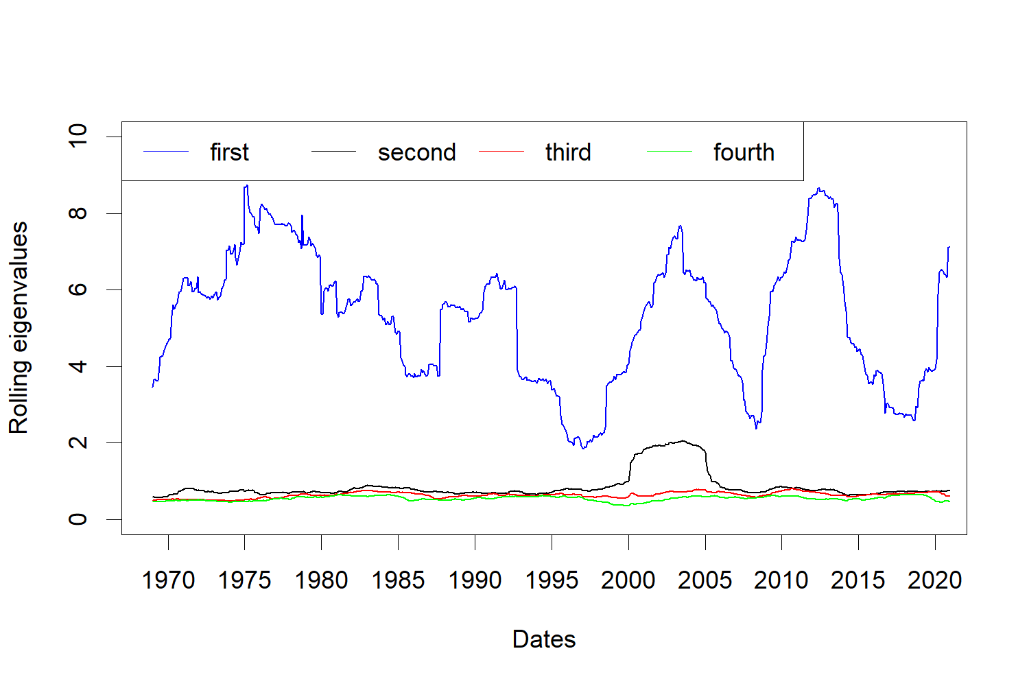
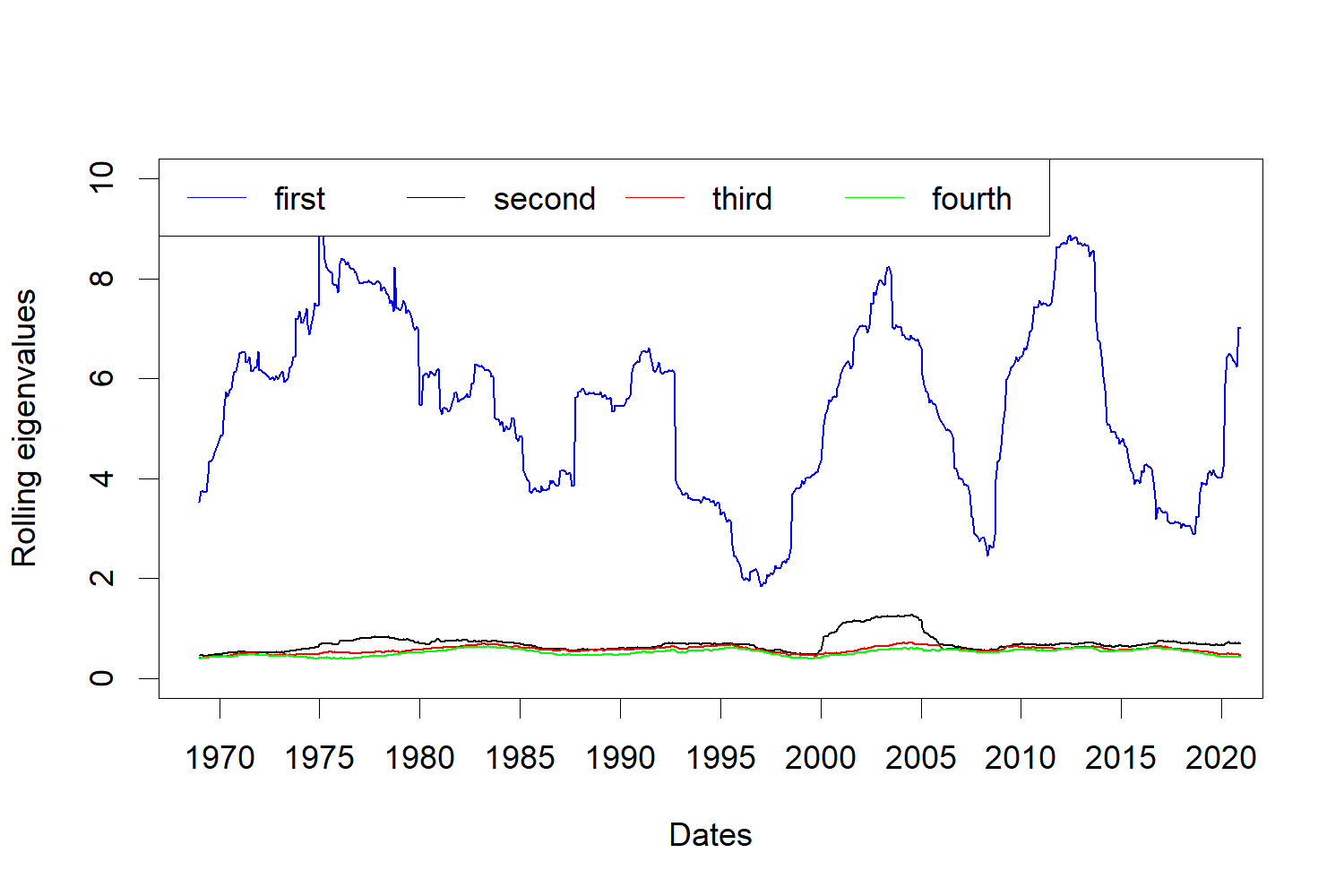
Figure 1: Eigenvalues of the rolling column-column and row-row sample covariance matrices in the monitoring. Left: column-column (for $k_{1}$); right: row-row (for $k_{2}$).

We implement our procedures at significance level $\alpha=0.05$, using, as sampling period, $m=60$ ($5$ years) for all the monitoring schemes. The first step of our analysis is to determine the number of row factor $k_{1}$. It turns out the numbers of row and column factors are both found to be equal to $1$, both when using the iterative algorithm in Yu et al. (2021), and the randomized testing procedure in He et al. (2021). Therefore, we start with $k_{1}=k_{2}=1$ for the monitoring procedure. Figure 1 illustrates the four leading eigenvalues of the rolling column-column and row-row projected sample covariance matrices. As shown in Figure 1, the first largest eigenvalue is always much larger than the remaining ones.

Our monitoring scheme detects, simultaneously, both changepoints in the factor loading spaces, and in the number of factor. As a leading example, we consider changes in the row factors, using the partial-sum testing statistics with $\eta=0$. As $p_{1}$ and $p_{2}$ are much smaller than those in our simulations, we use a larger $\delta=0.4$ when rescaling the eigenvalues, to reduce the effects of the noises, but still use the transformation function $g(x)=[\exp(x)-1]^{4}$. By way of robustness check, we repeat the testing procedures $100$ times, and declare a change point only when over $80\%$ of replications reject the corresponding null hypothesis. The change point is viewed to be located at the median of values from $100$ replications. We monitor until a changepoint is found, and, whenever a change point is detected, e.g., at $\hat{\tau}_{j}$, until the length of the remaining portion of the sample is smaller than $m$.

In the first step, we monitor the second largest eigenvalue of the rolling column-column projected sample covariance matrix from $t=m+1$ to the end of the sequence. The testing procedure outputs a change point in March 2003. We also monitor the first eigenvalue, using the procedure suggested in Section 4.1 to detect other types of change. In this case, we set $\tilde{g}(x)=1/g(x)$, finding no evidence of changepoints. Combining the results illustrated by Figure 1, it is apparent that a new factor emerges at $\tau_{1}=\text{\textquotedblleft March 2003\textquotedblright, with the second }$largest eigenvalue increasing significantly during this period. Subsequently, we restart the monitoring process from $t=\tau_{1}+1$, using $k_{1}=2$, monitoring the third and second largest eigenvalues. Interestingly, using the procedure proposed Section 4.1, we find evidence that the number of common factors drops to $1$ at $\tau_{2}$= “June 2008”. This date is highly suggestive, as it points towards concluding that, during the last global financial crisis, the number of common factors reduced. This finding can be read in conjunction with the empirical analysis in Massacci et al. (2021), where the number of common factors (albeit in a vector factor model with a threshold structure) is found to decrease during downside market regimes; as the authors put it, “diversification disappears when needed most”.

The change point locations for the row factors are plotted in the left panel of Figure 2, together with the maximum, median, and minimum returns series after standardization. The red vertical line indicates the time point when a new factor occurs, while the blue one indicates the time point when a factor disappears. The estimated locations are very close to the starting and ending points when the second largest eigenvalue increases and decreases in Figure 1. Also, as expected, the return series undergo a significant drop at the end of this period, say, the year 2008.

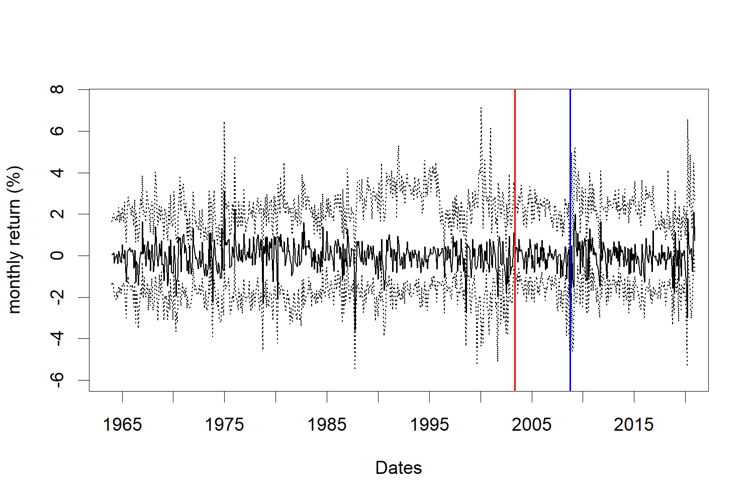
Figure 2: Illustration of the change points for the Fama-French 100 portfolio series by partial-sum monitoring procedure with $\eta=0$. Left: row factors; right: column factors. In each panel, the dash lines are the maximum and minimum return series, while the real line is the median return. The red and blue vertical lines are the change point locations when the number of factors increases and decreases, respectively.

As far as the column factors are concerned, we can run our procedure in parallel to detect any changes. However, by Figure 1, the second largest eigenvalue in the right panel grows, but not as significantly as in the left panel. Indeed, the monitoring procedure fails to detect any change point for column factors if we still use the same $g(x)$ and $\tilde{g}(x)$ as for the row factors, and therefore there seems to be no sufficient evidence to assert that the column loadings change during the monitoring period. Again for robustness, we slightly modified the function $g(x)$, to $g(x)=[\exp(x)-1]^{2}$ and $\tilde{g}(x)=1/g(x)$; in this case, we point out that our monitoring procedures do find evidence of two changepoints, as plotted in the right panel of Figure 2, whose locations are very close to those found for the row factors. This suggests that, if changepoints in the column factor spaces do exist, they are less evident and “pervasive” than in the case of the row factor space.

Table 4: Locations of change points detected by different monitoring procedures. The numbers in bracket indicates the type of change for the factor numbers, where “1” indicates new factor emerges; “-1” indicates a factor disappears while “NA” indicates no change.

	Change points	Partia-sum					Worst-case
		$\eta=0$	$\eta=0.25$	$\eta=0.5$	$\eta=0.65$	$\eta=0.75$
Row factors	First	March 2003(1)	March 2002(1)	December 2003(1)	NA	NA	NA
	Second	June 2008(-1)	April 2007(-1)	January 2009(-1)	NA	NA	NA
Column factors	First	May 2003(1)	December 2002(1)	NA	NA	NA	NA
	Second	October 2008(-1)	February 2008(-1)	NA	NA	NA	NA

We also repeated the above procedure using partial-sum statistics with different $\eta$, and the worst-case scenario statistic. Whilst, as can be expected, changepoints are not always detected by all procedures, it turns out that at most two change points are detected with all our monitoring schemes; we summarize our findings in Table 4, from which we can conclude the results are, broadly, not sensitive to the monitoring procedures.

6.2 Multinational macroeconomic indices

In this application, we study changepoint detection with macro data. We use the same data set as in Yu et al. (2021), which contains quarterly observations for $10$ macroeconomic indices over $8$ countries from 1988-Q1 to 2020-Q2. Similar data sets have also been studied in Liu and Chen (2019b) and Wang et al. (2019), which involves macroeconomic indices from more countries. We refer to Yu et al. (2021) for further details on the dataset, and the preprocessing steps.

The first step is to determine the numbers of row and column factors. In Figure 3, we also plot the leading five sample eigenvalues in the rolling monitoring process as in the first real example. Using the randomized testing procedures in He et al. (2021) suggests $k_{1}=1$, $k_{2}=3$ or $k_{1}=2$, $k_{2}=4$, which essentially indicates that one row and one column factor may be weaker than the others. Combining this information with the eigenvalue gaps shown in Figure 3, we take $k_{1}=1$ and $k_{2}=3$.

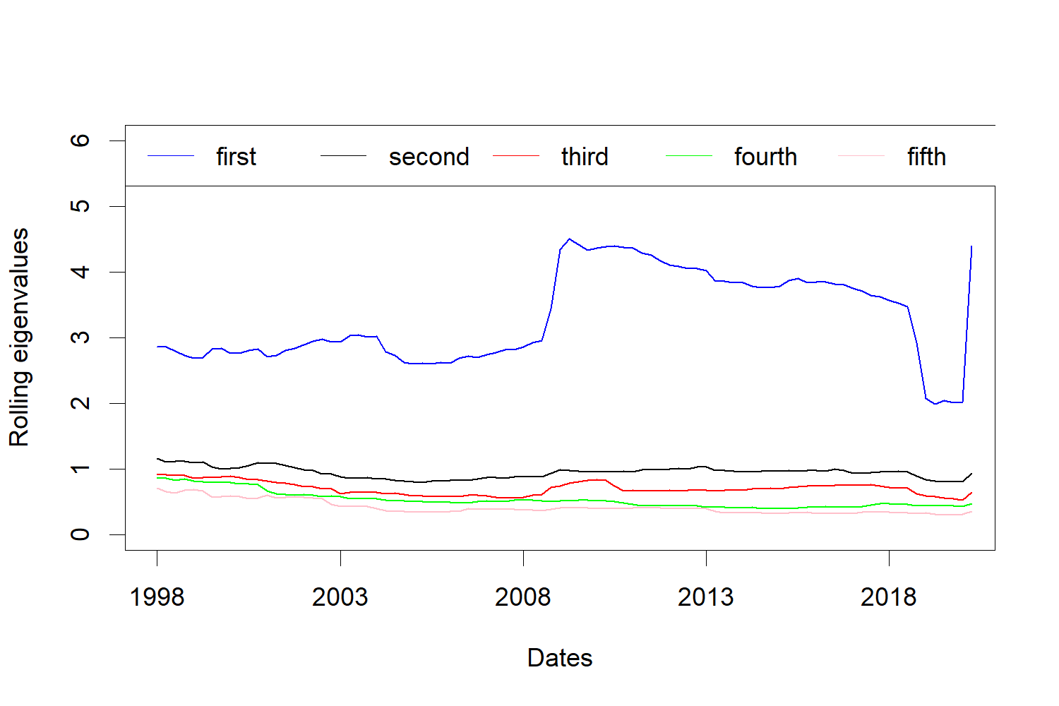
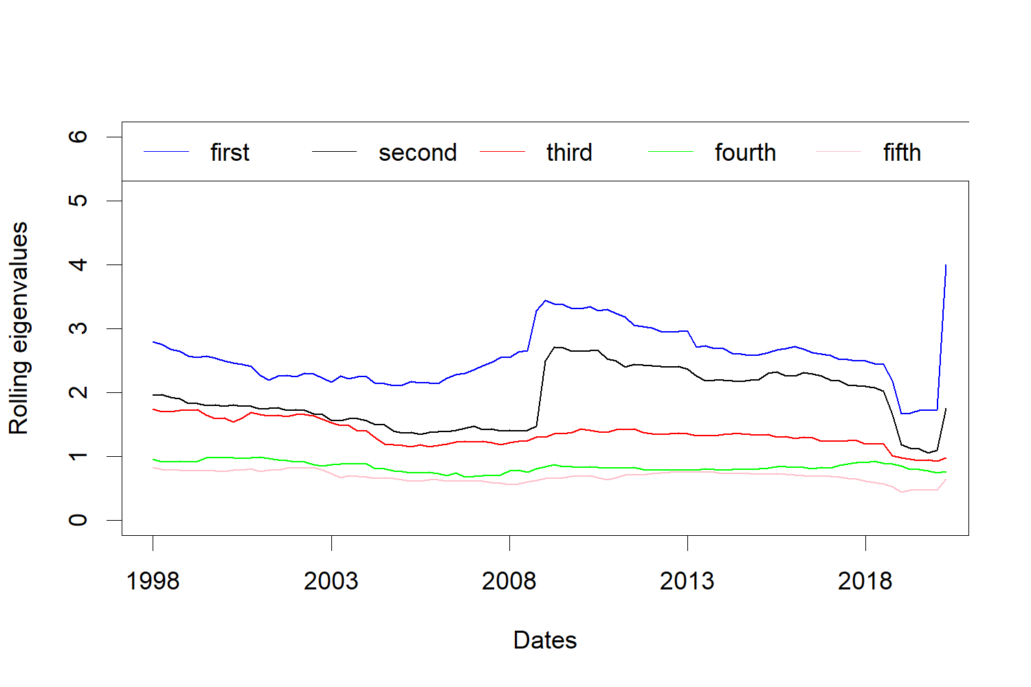
Figure 3: Eigenvalues of the rolling column-column and row-row sample covariance matrices in the monitoring for macroeconomic indices. Left: column-column (for $k_{1}$); right: row-row (for $k_{2}$).

In the second step, we use same approach as in the previous section to detect changepoints, i.e. we detect the change of factor loading spaces and the change of factor numbers simultaneously. We use $m=40$ ($10$ years), while setting the other tuning parameters the same as in the previous section, considering that $p_{1}$ and $p_{2}$ are of comparable size. For the partial-sum statistics with $\eta=0$, it turns out there are no change points for the row factors, while one column factor disappears in 2004-Q3. We plot the results in Figure 4, together with the median CPI series and median IR series. Interestingly, the location of the change point closely matches the changepoint detected in the previous example. On the other hand, by Figure 3, the third column eigenvalue (right panel) starts to decrease in the year 2004, and becomes relatively smaller than the leading two eigenvalues after the year 2008. Moreover, the CPI series becomes unstable after the year 2002, while the variance of IR series starts to decrease at the same time. Factoring in the possible delay in detection, this suggests a possible explanation for the 2004-Q3 break.

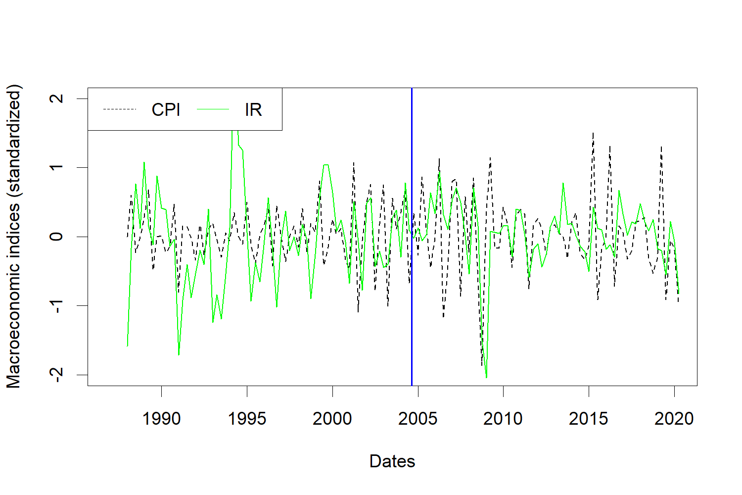
Figure 4: Illustration of the change point of column factors for macroeconomic indices. Black and green lines indicate the median CPI and interest rate series. Blue vertical line indicates the change point when a column factor disappears.

For other choices of $\eta$ and the worst-case statistic, we summarize the result in Table 5. Interestingly, the changepoints we detect in this example are all roughly close to the two change points detected in the previous example. We also remark that in this macroeconomic example, the length of series is much smaller than that in the last one. Actually, for the testing statistics with $\eta>0.5$, the effective sample size in the monitoring process is $\ln(T_{m})\leq\ln 90$, which is very small. Hence, in this example we prefer to trust the results from testing procedures with smaller $\eta$ or the worst-case testing procedure.

Table 5: Estimated change points locations by different monitoring procedures. The numbers -1 in brackets indicates a factor disappears. “NA” means no change point.

	Change points	Partia-sum					Worst-case
		$\eta=0$	$\eta=0.25$	$\eta=0.5$	$\eta=0.65$	$\eta=0.75$
Row factor	First	NA	NA	NA	NA	NA	NA
Column factor	First	2004-Q3(-1)	2003-Q1(-1)	2000-Q3(-1)	1999-Q2(-1)	1998-Q3(-1)	2008-Q3(-1)

7   Conclusions

In this paper, we have proposed several schemes for the online detection of changes in the latent factor structures of a two-way, matrix factor model. Our approach is based on noting that many instances of changepoint can be represented as a change in the dimension of the factor spaces. Hence, in order to detect changes, we use the eigenvalues of the projected second moment matrices, which diverge with the cross-sectional sample or not according to the number of common factors. Having a spiked behaviour in an eigenvalue which was bounded during a training period, or observing the vanishing of such a spiked behaviour, point towards the presence of a break. Since we do not know the limiting distribution of the estimated eigenvalues, which is likely to be very challenging to derive especially in the case where the eigenvalue is not spiked, we randomise the sequence of the estimated eigenvalue by perturbing it with an i.i.d., standard normal sequence. Thence, we are able to propose two families of sequential procedures, one more “classical” and based on the fluctuations of partial sums, and another one, completely novel, based on the extreme value behaviour of the perturbed sequence of estimated eigenvalues. Our approach has several distinctive advantages: it is easy to implement, it requires much less tuning than competing approaches (see e.g. Barigozzi and Trapani, 2020), and it works very well in simulations, offering good size control and fast changepoint detection. Indeed, whilst approaches based on partial sums work very well, the methodology based on the extreme value, worst-case scenario delivers an even superior performance, thus suggesting that our methodology could be very promising even in other, very different contexts.

Appendix A Further assumptions

The following assumptions are borrowed from the paper by Yu et al. (2021), to which we refer for detailed explanations and discussions.

Assumption B1.

(i) (a) $E(F_{t})=0$, and (b) $E\|F_{t}\|^{4+\epsilon}\leq c_{0}$, for some $\epsilon>0$; (ii)

$$\frac{1}{T}\sum_{t=1}^{T}F_{t}F_{t}^{\prime}\overset{a.s.}{\rightarrow}{\Sigma}_{1}\text{ and }\frac{1}{T}\sum_{t=1}^{T}F_{t}^{\prime}F_{t}\overset{a.s.}{\rightarrow}\Sigma_{2},$$ (A.1)

where $\Sigma_{i}$ is a $k_{i}\times k_{i}$ positive definite matrix with distinct eigenvalues and spectral decomposition $\Sigma_{i}=\Gamma_{i}\Lambda_{i}\Gamma_{i}^{\prime}$, $i=1,2$. The factor numbers $k_{1}$ and $k_{2}$ are fixed as $\min\{T,p_{1},p_{2}\}\rightarrow\infty$; (iii) it holds that, for all $1\leq h_{1},l_{1}\leq k_{1}$ and $1\leq h_{2},l_{2}\leq k_{2}$

$$E\max_{1\leq\widetilde{t}\leq T}\left(\sum_{t=1}^{\widetilde{t}}\left(F_{h_{1}h_{2},t}F_{l_{1}l_{2},t}-E\left(F_{h_{1}h_{2},t}F_{l_{1}l_{2},t}\right)\right)\right)^{2}\leq c_{0}T.$$

Assumption B2.

(i) $\|R\|_{\max}\leq c_{0}$, and $\|C\|_{\max}\leq c_{1}$; (ii) as $\min\{p_{1},p_{2}\}\rightarrow\infty$, $\|p_{1}^{-1}R^{\top}R-I_{k_{1}}\|\rightarrow 0$ and $\|p_{2}^{-1}C^{\top}C-I_{k_{2}}\|\rightarrow 0$.

Assumptions B1 and B2 are standard in large factor models, and we refer, for example, to Chen and Fan (2021). In Assumption B1(i)(b), note the (mild) strengthening of the customarily assumed fourth moment existence condition on $F_{t}$ - this is required in order to prove our results, which rely on almost sure rates. Similarly, the maximal inequality in part (iii) of the assumption is usually not considered in the literature, and it can be derived from more primitive dependence assumptions: for example, it can be shown to hold under various mixing conditions (see e.g. Rio, 1995; and Shao, 1995), and for the very general class of decomposable Bernoulli shifts (see e.g. Berkes et al., 2011; Liu and Lin, 2009; and Barigozzi and Trapani, 2021). Finally, we point out that, according to Assumption B2, the common factors are pervasive. Extensions to the case of “weak” factors go beyond the scope of this paper, but are in principle possible.

Assumption B3.

(i) (a) $E(e_{ij,t})=0$, and (b) $E(e_{ij,t}^{8})\leq c_{0}$; (ii) for all $1\leq t\leq T$, $1\leq i\leq p_{1}$ and $1\leq j\leq p_{2}$,

$$(\text{a}).\sum_{s=1}^{T}\sum_{l=1}^{p_{1}}\sum_{h=1}^{p_{2}}|E(e_{ij,t}e_{lh,s})|\leq c_{0},\quad(\text{b}).\sum_{l=1}^{p_{1}}\sum_{h=1}^{p_{2}}|{E}(e_{lj,t}e_{ih,t})|\leq c_{0};$$

(iii) for all $1\leq t\leq T$, $1\leq i\leq p_{1}$ and $1\leq j\leq p_{2}$,

$$\begin{array}[]{cl}\left(\text{a}\right).&\sum_{s=1}^{T}\sum_{l_{2}=1}^{p_{1}}\sum_{h=1}^{p_{2}}\left|Cov(e_{ij,t}e_{l_{1}j,t},e_{ih,s}e_{l_{2}h,s})\right|\leq c_{0},\\ &\sum_{s=1}^{T}\sum_{l=1}^{p_{1}}\sum_{h_{2}=1}^{p_{2}}\left|Cov(e_{ij,t}e_{ih_{1},t},e_{lj,s}e_{lh_{2},s})\right|\leq c_{0},\\ &\sum_{s=1}^{T}\sum_{l=1}^{p_{1}}\sum_{h=1}^{p_{2}}\left|Cov(e_{ij,t}^{2},e_{lh,s}^{2})\right|\leq c_{0},\\ \left(\text{b}\right).&\sum_{s=1}^{T}\sum_{l_{2}=1}^{p_{1}}\sum_{h_{2}=1}^{p_{2}}\left|Cov(e_{ij,t}e_{l_{1}h_{1},t},e_{ij,s}e_{l_{2}h_{2},s})+Cov(e_{l_{1}j,t}e_{ih_{1},t},e_{l_{2}j,s}e_{ih_{2},s})\right|\leq c_{0},\end{array}$$

(iv) it holds that $\lambda_{\min}\left[E\left(\frac{1}{p_{2}T}\sum_{t=1}^{T}E_{t}E_{t}^{\prime}\right)\right]>0$ and $\lambda_{\min}\left[E\left(\frac{1}{p_{1}T}\sum_{t=1}^{T}E_{t}^{\prime}E_{t}\right)\right]>0$.

Assumption B3 ensures the (cross-sectional and time series) summability of the idiosyncratic terms $E_{t}$. The assumption requires weak dependence in both the space and time domains; in principle, it is possible to show that this assumption is satisfied for many dependence assumptions and data generating processes. The assumption can be read in conjunction with the paper by Wang et al. (2019), where $E_{t}$ is assumed to be white noise, which can be viewed as overly restrictive.

Assumption B4.

(i) For any deterministic vectors ${v}$ and ${w}$ satisfying $\|{v}\|=1$ and $\|{w}\|=1$ with suitable dimensions,

$${E}\bigg{\|}\frac{1}{\sqrt{T}}\sum_{t=1}^{T}F_{t}({v}^{\prime}E_{t}{w})\bigg{\|}^{2}\leq c_{0};$$

(ii) for all $1\leq i,l_{1}\leq p_{1}$ and $1\leq j,h_{1}\leq p_{2}$,

$$\begin{split}&(\text{a}).\Big{\|}\sum_{h=1}^{p_{2}}{E}(\bar{\zeta}_{ij}\otimes\bar{\zeta}_{ih})\Big{\|}_{\max}\leq c_{0},\quad\Big{\|}\sum_{l=1}^{p_{1}}{E}(\bar{\zeta}_{ij}\otimes\bar{\zeta}_{lj})\Big{\|}_{\max}\leq c_{0},\\ &(\text{b}).\Big{\|}\sum_{l=1}^{p_{1}}\sum_{h_{2}=1}^{p_{2}}Cov(\bar{\zeta}_{ij}\otimes\bar{\zeta}_{ih_{1}},\bar{\zeta}_{lj}\otimes\bar{\zeta}_{lh_{2}})\Big{\|}_{\max}\leq c_{0},\Big{\|}\sum_{l_{2}=1}^{p_{1}}\sum_{h=1}^{p_{2}}Cov(\bar{\zeta}_{ij}\otimes\bar{\zeta}_{l_{1}j},\bar{\zeta}_{ih}\otimes\bar{\zeta}_{l_{2}h})\Big{\|}_{\max}\leq c_{0},\end{split}$$

where $\bar{\zeta}_{ij}=\text{Vec}(\sum_{t=1}^{T}F_{t}e_{ij,t}/\sqrt{T})$.

According to Assumption B4, the common factors $F_{t}$ and the errors $E_{t}$ can be weakly correlated. The assumption holds under the more restrictive case that $\{F_{t}\}$ and $\{E_{t}\}$ are two mutually independent groups.

A.1 Technical lemmas and proofs

Lemma B.1.

We assume that Assumptions B1-B4 are satisfied. Then it holds that there exist a triplet of random variables $\left(p_{1,0},p_{2,0},m_{0}\right)$ such that

(i)

under (3.7)

$$\widehat{\lambda}_{k_{1}+1,\tau}\left\{\begin{array}[]{ll}\leq c_{0}&\text{for }\tau\leq t^{\ast}\\ \geq c_{1}\min\left(\frac{\tau-t^{\ast}}{m},\frac{m+t^{\ast}-\tau}{m}\right)p_{1}&\text{for }t^{\ast}<\tau<m+t^{\ast}\\ \leq c_{0}&\text{for }\tau\geq m+t^{\ast}\end{array}\right.;$$

(ii)

under (3.9)

$$\widehat{\lambda}_{k_{1}+1,\tau}\left\{\begin{array}[]{ll}\leq c_{0}&\text{for }\tau\leq t^{\ast}\\ \geq c_{1}\frac{\tau-t^{\ast}}{m}p_{1}&\text{for }t^{\ast}<\tau<m+t^{\ast}\\ \geq c_{0}p_{1}&\text{for }\tau\geq m+t^{\ast}\end{array}\right..$$

Proof.

The proof of the lemma is based on very similar passages as the proof of Lemma 1 in Barigozzi and Trapani (2020), and thus we report only the main passages. We begin with part (ii) of the lemma, focusing on the case $t^{\ast}<\tau<m+t^{\ast}$. Note that

$$\widehat{\lambda}_{k_{1}+1,\tau} = \widehat{\lambda}_{k_{1}+1}\left(\frac{1}{m}\sum_{t=\tau+1}^{m+t^{\ast}}Y_{t}Y_{t}^{\prime}+\frac{1}{m}\sum_{t=m+t^{\ast}}^{m+\tau}Y_{t}Y_{t}^{\prime}\right)$$

$$\geq \widehat{\lambda}_{\min}\left(\frac{1}{m}\sum_{t=\tau+1}^{m+t^{\ast}}Y_{t}Y_{t}^{\prime}\right)+\widehat{\lambda}_{k_{1}+1}\left(\frac{1}{m}\sum_{t=m+t^{\ast}}^{m+\tau}Y_{t}Y_{t}^{\prime}\right)$$

$$\geq \widehat{\lambda}_{k_{1}+1}\left(\frac{1}{m}\sum_{t=m+t^{\ast}}^{m+\tau}Y_{t}Y_{t}^{\prime}\right),$$

by Weyl’s inequality. Also

$$\widehat{\lambda}_{k_{1}+1}\left(\frac{1}{m}\sum_{t=m+t^{\ast}}^{m+\tau}Y_{t}Y_{t}^{\prime}\right)=\frac{\tau-t^{\ast}}{m}\widehat{\lambda}_{k_{1}+1}\left(\frac{1}{m+\tau-t^{\ast}}\sum_{t=m+t^{\ast}}^{m+\tau}Y_{t}Y_{t}^{\prime}\right);$$

the fact that

$$\widehat{\lambda}_{k_{1}+1}\left(\frac{1}{\tau-t^{\ast}}\sum_{t=m+t^{\ast}}^{m+\tau}Y_{t}Y_{t}^{\prime}\right)\geq c_{0}p_{1},$$

is an immediate consequence of Lemma 1. The rest of the proof - for the cases $\tau\leq t^{\ast}$ and $\tau\geq m+t^{\ast}$ - follows immediately. We now turn to part (i) of the Lemma, and consider the case where all loadings change for simplicity - i.e. $R_{0}$ is empty. In the interval $t^{\ast}<\tau<m+t^{\ast}$ we can write

$$X_{t}=\left[\begin{array}[]{cc}R_{1}&R_{2}\end{array}\right]\left[\begin{array}[]{cc}F_{t}I\left(t<t^{\ast}\right)&0\\ 0&F_{t}I\left(t\geq t^{\ast}\right)\end{array}\right]\left[\begin{array}[]{c}C^{\prime}\\ C^{\prime}\end{array}\right]+E_{t}.$$

The second moment matrix has a component given by

$$\left[\begin{array}[]{cc}\frac{1}{m}\sum_{t=\tau+1}^{m+t^{\ast}}R_{1}F_{t}I\left(t<t^{\ast}\right)C^{\prime}\widehat{C}\widehat{C}^{\prime}CF_{t}^{\prime}R_{1}^{\prime}&0\\ 0&\frac{1}{m}\sum_{t=m+t^{\ast}}^{m+\tau}R_{2}F_{t}I\left(t\geq t^{\ast}\right)C^{\prime}\widehat{C}\widehat{C}^{\prime}CF_{t}^{\prime}R_{2}^{\prime}\end{array}\right]$$

The spectrum of this matrix is the union of the spectra of the two blocks, and therefore, using Lemma 1, it follows that

$$\widehat{\lambda}_{k_{1}+1}\left(\frac{1}{m}\sum_{t=m+t^{\ast}}^{m+\tau}Y_{t}Y_{t}^{\prime}\right)$$

$$\geq c_{0}\min\left\{\widehat{\lambda}_{k_{1}}\left(\frac{1}{m}\sum_{t=\tau+1}^{m+t^{\ast}}R_{1}F_{t}I\left(t<t^{\ast}\right)C^{\prime}\widehat{C}\widehat{C}^{\prime}CF_{t}^{\prime}R_{1}^{\prime}\right),\widehat{\lambda}_{k_{1}}\left(\frac{1}{m}\sum_{t=m+t^{\ast}}^{m+\tau}R_{2}F_{t}I\left(t\geq t^{\ast}\right)C^{\prime}\widehat{C}\widehat{C}^{\prime}CF_{t}^{\prime}R_{2}^{\prime}\right)\right\}$$

$$\geq c_{0}\min\left\{\frac{m+t^{\ast}-\tau}{m},\frac{\tau-t^{\ast}}{m}\right\},$$

whence the desired result follows. ∎

Proof of Theorem 1.

We begin by showing (3.22), where $\eta<1/2$. Define

$$S_{\tau}^{\ast}=\sum_{j=1}^{\tau}z_{j},$$

and recall that $\left\{z_{\tau},1\leq\tau\leq T_{m}\right\}$ is i.i.d. $N\left(0,1\right)$. Since $\psi_{\tau}\geq 0$ for all $\tau$, it holds that

$$\max_{1\leq\tau\leq T_{m}}\frac{\left|S_{\tau}-S_{\tau}^{\ast}\right|}{\tau^{\eta}}=\max_{1\leq\tau\leq T_{m}}\frac{\sum_{j=1}^{\tau}\psi_{j}}{\tau^{\eta}}=T_{m}^{1-\eta}g\left(p_{1}^{-\delta}\frac{p_{1}}{T^{1/2}}\left(\ln p_{1}\right)^{1+\epsilon}\left(\ln p_{2}\right)^{1+\epsilon}\left(\ln T\right)^{1+\epsilon}\right)=o_{P^{\ast}}\left(1\right),$$ (B.1)

due to (3.17). By the KMT approximation (see Komlós et al., 1975, and Komlós et al., 1976), there exists a sequence of standard Wiener process $W_{T_{m}}\left(x\right)$, $0<x<\infty$, such that

$$\max_{1\leq\tau\leq T_{m}}\frac{1}{\ln\tau}\left|S_{\tau}^{\ast}-W_{T_{m}}\left(\tau\right)\right|=O_{P}\left(1\right).$$ (B.2)

Then, using (B.2), it follows that

$$T_{m}^{\eta-1/2}\max_{1\leq\tau\leq Tm}\tau^{-\eta}\left|S_{\tau}^{\ast}-W_{T_{m}}\left(\tau\right)\right|$$

$$\leq T_{m}^{\eta-1/2}\max_{1\leq\tau\leq Tm}\frac{1}{\ln\tau}\left|S_{\tau}^{\ast}-W_{T_{m}}\left(\tau\right)\right|\max_{1\leq\tau\leq Tm}\tau^{-\eta}\ln\tau$$

$$= o_{P}\left(1\right).$$

Finally

$$T_{m}^{\eta-1/2}\max_{1\leq\tau\leq Tm}\tau^{-\eta}\left|W_{T_{m}}\left(\tau\right)\right|$$

$$= \max_{1\leq\tau\leq Tm}\left(\frac{\tau}{T_{m}}\right)^{-\eta}\left|W_{T_{m}}\left(\frac{\tau}{T_{m}}\right)\right|$$

$$\overset{D}{=}\max_{1/T_{m}\leq u\leq 1}\left(u\right)^{-\eta}\left|W\left(u\right)\right|$$

$$\overset{a.s.}{\rightarrow}\max_{0\leq u\leq 1}\left(u\right)^{-\eta}\left|W\left(u\right)\right|,$$

as $T_{m}\rightarrow\infty$, having used the scale transformation of the Wiener process. Putting (B.1), (B.2), (A.1) and (A.1) together, (3.22) follows.

We now turn to showing (3.23). Note first that

$$\left|\max_{1\leq\tau\leq T_{m}}\tau^{-1/2}\left|S_{\tau}\right|-\max_{1\leq\tau\leq T_{m}}\tau^{-1/2}\left|S_{\tau}^{\ast}\right|\right|$$

$$\leq \max_{1\leq\tau\leq T_{m}}\tau^{-1/2}\sum_{j=1}^{\tau}\psi_{j}$$

$$\leq T_{m}^{-1/2}\sum_{j=1}^{T_{m}}\psi_{j}=O_{a.s.}\left(T_{m}^{1/2}g\left(p_{1}^{-\delta}\frac{p_{1}}{T^{1/2}}\left(\ln p_{1}\right)^{1+\epsilon}\left(\ln p_{2}\right)^{1+\epsilon}\left(\ln T\right)^{1+\epsilon}\right)\right)$$

$$= o_{a.s.}\left(T_{m}^{-1/2}\right),$$

having used (3.11) and (3.17). Thus it holds that

$$\alpha_{Tm}\left|\max_{1\leq\tau\leq T_{m}}\left|S_{\tau}\right|-\max_{1\leq\tau\leq T_{m}}\left|S_{\tau}^{\ast}\right|\right|-\beta_{Tm}\overset{a.s.}{\rightarrow}-\infty;$$ (B.5)

this proves equation (2.3) in Shorack (1979). Hence

$$P^{\ast}\left(\alpha_{Tm}\max_{1\leq\tau\leq T_{m}}\tau^{-1/2}\left|S_{\tau}\right|\leq x+\beta_{Tm}\right)=P^{\ast}\left(\alpha_{Tm}\max_{1\leq\tau\leq T_{m}}\tau^{-1/2}\left|S_{\tau}^{\ast}\right|\leq x+\beta_{Tm}\right)+o_{P^{\ast}}\left(1\right);$$

recalling that $S_{\tau}^{\ast}$ is the partial sums process of a sequence of i.i.d. standard normals, the Darling-Erdős theorem (Darling and Erdős, 1956) yields the desired result.

Finally, we show (3.24). The proof is similar to the above, so we omit passages when this does not cause confusion. Note that

$$r_{T_{m}}^{\eta-1/2}\left|\max_{r_{T_{m}}\leq\tau\leq T_{m}}\tau^{-\eta}\left|S_{\tau}\right|-\max_{r_{T_{m}}\leq\tau\leq T_{m}}\tau^{-\eta}\left|S_{\tau}^{\ast}\right|\right|$$

$$\leq r_{T_{m}}^{\eta-1/2}\max_{r_{T_{m}}\leq\tau\leq T_{m}}\tau^{-\eta}\sum_{j=1}^{\tau}\psi_{j},$$

which is bounded by

$$O_{a.s.}\left(r_{T_{m}}^{\eta-1/2}T_{m}^{1-\eta}g\left(p_{1}^{-\delta}\frac{p_{1}}{T^{1/2}}\left(\ln p_{1}\right)^{1+\epsilon}\left(\ln p_{2}\right)^{1+\epsilon}\left(\ln T\right)^{1+\epsilon}\right)\right),$$

whenever $\frac{1}{2}<\eta<1$, and by

$$O_{a.s.}\left(r_{T_{m}}^{1/2}g\left(p_{1}^{-\delta}\frac{p_{1}}{T^{1/2}}\left(\ln p_{1}\right)^{1+\epsilon}\left(\ln p_{2}\right)^{1+\epsilon}\left(\ln T\right)^{1+\epsilon}\right)\right),$$

when $\eta>1$. In both cases, it is easy to see that the bounds drift to zero as $\min\left(p_{1},p_{2},T\right)\rightarrow\infty$. Also

$$r_{T_{m}}^{\eta-1/2}\max_{r_{T_{m}}\leq\tau\leq T_{m}}\tau^{-\eta}\left|S_{\tau}^{\ast}-W_{T_{m}}\left(\tau\right)\right|$$

$$\leq r_{T_{m}}^{\eta-1/2}\max_{r_{T_{m}}\leq\tau\leq T_{m}}\tau^{-\eta}\frac{\left|S_{\tau}^{\ast}-W_{T_{m}}\left(\tau\right)\right|}{\ln\tau}\ln\tau$$

$$\leq O_{P}\left(1\right)r_{T_{m}}^{\eta-1/2}\max_{r_{T_{m}}\leq\tau\leq T_{m}}\tau^{-\eta}\ln\tau$$

$$= O_{P}\left(r_{T_{m}}^{-1/2}\ln r_{T_{m}}\right)=o_{P}\left(1\right),$$

where $S_{\tau}^{\ast}$ and $W_{T_{m}}\left(\tau\right)$ are defined above. Hence we need to study

$$r_{T_{m}}^{\eta-1/2}\max_{r_{T_{m}}\leq\tau\leq T_{m}}\tau^{-\eta}\left|W_{T_{m}}\left(\tau\right)\right|;$$

using the scale transformation, we obtain

$$r_{T_{m}}^{\eta-1/2}\max_{r_{T_{m}}\leq\tau\leq T_{m}}\tau^{-\eta}\left|W_{T_{m}}\left(\tau\right)\right|\overset{D}{=}\left(\frac{r_{T_{m}}}{T_{m}}\right)^{\eta-1/2}\max_{\frac{r_{T_{m}}}{T_{m}}\leq t\leq 1}t^{-\eta}\left|W\left(t\right)\right|;$$

setting $s=t\frac{T_{m}}{r_{T_{m}}}$, and using again the scale transformation

$$\left(\frac{r_{T_{m}}}{T_{m}}\right)^{\eta-1/2}\max_{\frac{r_{T_{m}}}{T_{m}}\leq t\leq 1}t^{-\eta}\left|W\left(t\right)\right|\overset{D}{=}\max_{1\leq s\leq\frac{T_{m}}{r_{T_{m}}}}s^{-\eta}\left|W\left(s\right)\right|\overset{a.s.}{\rightarrow}\sup_{1\leq s<\infty}\frac{\left|W\left(s\right)\right|}{s^{\eta}},$$

completing the proof. ∎

Proof of Theorem 2.

We write

$$S_{\tau}=\sum_{j=1}^{\tau}z_{j}+\sum_{j=1}^{t^{\ast}}\psi_{j}+\sum_{j=t^{\ast}+1}^{\tau}\psi_{j},$$

with the convention that $\sum_{c}^{d}=0$ whenever $d<c$, and we begin by observing that, under (3.7), (3.8) entails that there are two numbers $0<a<b<1$ such that there exists a triplet of random variables $\left(p_{1,0},p_{2,0},T_{0}\right)$ and a positive constant $c_{0}$ such that, for $p_{1}\geq p_{1,0}$, $p_{2}\geq p_{2,0}$ and $T\geq T_{0}$

$$\widehat{\lambda}_{k_{1}+1,\tau}\geq c_{0}p_{1}\text{ for }t^{\ast}+am\leq\tau\leq t^{\ast}+m-bm.$$ (B.6)

We now turn to proving the theorem. Consider first the case $0\leq\eta<\frac{1}{2}$, and note that, by the Law of the Iterated Logarithm

$$T_{m}^{\eta-1/2}\max_{1\leq\tau\leq T_{m}}\tau^{-\eta}\sum_{j=1}^{\tau}z_{j}=O_{a.s.}\left(\sqrt{\ln\ln T_{m}}\right);$$

also

$$T_{m}^{\eta-1/2}\max_{1\leq\tau\leq T_{m}}\tau^{-\eta}\sum_{j=1}^{t^{\ast}}\psi_{j}=o_{a.s.}\left(T_{m}^{\eta+1/2}g\left(\frac{p_{1}^{1-\delta}}{m^{1/2}}\left(\ln p_{1}\right)^{1+\epsilon}\left(\ln p_{2}\right)^{1+\epsilon}\left(\ln m\right)^{1+\epsilon}\right)\right)=o_{a.s.}\left(1\right),$$

on account of (3.17). Finally, by (B.6), there exists a triplet of random variables $\left(p_{1,0},p_{2,0},T_{0}\right)$ and a positive constant $c_{0}$ such that, for $p_{1}\geq p_{1,0}$, $p_{2}\geq p_{2,0}$ and $T\geq T_{0}$

$$\max_{1\leq\tau\leq T_{m}}\tau^{-\eta}\sum_{j=t^{\ast}+1}^{\tau}\psi_{j}$$

$$\geq \max_{1\leq\tau\leq T_{m}}\tau^{-\eta}\sum_{j=am+t^{\ast}+1}^{\tau}\psi_{j}$$

$$\geq c_{0}g\left(p_{1}^{1-\delta}\right)\max_{t^{\ast}+1\leq\tau\leq m+t^{\ast}}\tau^{-\eta}\left(\tau-t^{\ast}\right)$$

$$= c_{1}g\left(p_{1}^{1-\delta}\right)\left(t^{\ast}\right)^{1-\eta},$$

where the last result follows from standard algebra, and it is valid for all $\eta$. Now (3.25) follows putting everything together. When $\eta>1/2$, essentially the same arguments yield

$$r_{T_{m}}^{\eta-1/2}\max_{r_{T_{m}}\leq\tau\leq T_{m}}\tau^{-\eta}\sum_{j=1}^{\tau}z_{j} = O_{a.s.}\left(\sqrt{\ln\ln T_{m}}\right),$$

$$r_{T_{m}}^{\eta-1/2}\max_{r_{T_{m}}\leq\tau\leq T_{m}}\tau^{-\eta}\sum_{j=1}^{t^{\ast}}\psi_{j} = o_{a.s.}\left(r_{T_{m}}^{-1/2}t^{\ast}g\left(\frac{p_{1}^{1-\delta}}{m^{1/2}}\left(\ln p_{1}\right)^{1+\epsilon}\left(\ln p_{2}\right)^{1+\epsilon}\left(\ln m\right)^{1+\epsilon}\right)\right)=o_{a.s.}\left(1\right).$$

Equation (3.29) follows by putting these results and (A.1) together. Finally, when $\eta=1/2$, it is easy to see by the same logic as above that

$$\max_{1\leq\tau\leq T_{m}}\tau^{-1/2}\sum_{j=1}^{\tau}z_{j} = O_{a.s.}\left(\sqrt{\ln\ln T_{m}}\right),$$

$$\max_{1\leq\tau\leq T_{m}}\tau^{-1/2}\sum_{j=1}^{t^{\ast}}\psi_{j} = o_{a.s.}\left(t^{\ast}g\left(\frac{p_{1}^{1-\delta}}{m^{1/2}}\left(\ln p_{1}\right)^{1+\epsilon}\left(\ln p_{2}\right)^{1+\epsilon}\left(\ln m\right)^{1+\epsilon}\right)\right)=o_{a.s.}\left(1\right),$$

so that (3.27) follows from the same logic as above. Under (3.9), the proof uses essentially the same arguments, with the only difference that, by (3.10), there is a number $0<a<1$ such that there exists a triplet of random variables $\left(p_{1,0},p_{2,0},T_{0}\right)$ and a positive constant $c_{0}$ such that, for $p_{1}\geq p_{1,0}$, $p_{2}\geq p_{2,0}$ and $T\geq T_{0}$

$$\widehat{\lambda}_{k_{1}+1,\tau}\geq c_{0}p_{1}\text{ for }t^{\ast}+am\leq\tau\leq T_{m}.$$

∎

Proof of Theorem 3.

We will use the short-hand notation

$$Z_{Tm}=\max_{1\leq\tau\leq T_{m}}y_{\tau}.$$

Note that

$$P^{\ast}\left(\frac{Z_{Tm}-b_{Tm}}{a_{Tm}}\leq v\right)=P^{\ast}\left(Z_{Tm}\leq a_{Tm}v+b_{Tm}\right),$$

and consider the sequence $y_{\tau}$ defined in (3.16), viz.

$$y_{\tau}=z_{\tau}+\psi_{\tau}.$$

By construction, $z_{\tau}$ is independent across $\tau$ and independent of the sample $\left\{X_{t},1\leq t\leq T+T_{m}\right\}$. Hence, letting $\Phi\left(\cdot\right)$ be the distribution of the standard normal and $\varphi\left(\cdot\right)$ its density, we can write

$$P^{\ast}\left(Z_{Tm}\leq a_{Tm}v+b_{Tm}\right) = \prod\limits_{\tau=1}^{T_{m}}P^{\ast}\left(y_{\tau}\leq a_{Tm}v+b_{Tm}\right)$$

$$= \prod\limits_{\tau=1}^{T_{m}}P^{\ast}\left(z_{\tau}\leq a_{Tm}v+b_{Tm}-\psi_{\tau}\right)$$

$$= \exp\left(\sum_{\tau=1}^{T_{m}}\ln\Phi\left(a_{Tm}v+b_{Tm}-\psi_{\tau}\right)\right).$$

Note that

$$\ln\Phi\left(a_{Tm}v+b_{Tm}-\psi_{\tau}\right)=\ln\Phi\left(a_{Tm}v+b_{Tm}\right)+\ln\frac{\Phi\left(a_{Tm}v+b_{Tm}-\psi_{\tau}\right)}{\Phi\left(a_{Tm}v+b_{Tm}\right)}.$$ (B.9)

Using Taylor’s expansion, for some $c_{0}>0$ it holds that

$$\ln\Phi\left(a_{Tm}v+b_{Tm}-\psi_{\tau}\right) = \ln\Phi\left(a_{Tm}v+b_{Tm}\right)+\ln\frac{\Phi\left(a_{Tm}v+b_{Tm}-\psi_{\tau}\right)}{\Phi\left(a_{Tm}v+b_{Tm}\right)}$$

$$= \ln\Phi\left(a_{Tm}v+b_{Tm}\right)+\ln\left[1-c_{0}\psi_{\tau}\frac{\varphi\left(a_{Tm}v+b_{Tm}\right)}{\Phi\left(a_{Tm}v+b_{Tm}\right)}\right].$$

Therefore, putting together (A.1)-(A.1)

$$P^{\ast}\left(Z_{Tm}\leq a_{Tm}v+b_{Tm}\right)$$

$$= \exp\left(\sum_{\tau=1}^{T_{m}}\ln\Phi\left(a_{Tm}v+b_{Tm}-\psi_{\tau}\right)\right)$$

$$= \exp\left(\sum_{\tau=1}^{T_{m}}\ln\Phi\left(a_{Tm}v+b_{Tm}\right)\right)\exp\left(\sum_{\tau=1}^{T_{m}}\ln\left[1-c_{0}\psi_{\tau}\frac{\varphi\left(a_{Tm}v+b_{Tm}\right)}{\Phi\left(a_{Tm}v+b_{Tm}\right)}\right]\right)$$

$$= \left[\Phi\left(a_{Tm}v+b_{Tm}\right)\right]^{T_{m}}\exp\left(\sum_{\tau=1}^{T_{m}}\ln\left[1-c_{1}\psi_{\tau}\right]\right).$$

Consider the elementary inequality $\ln\left(1-c_{1}\psi_{\tau}\right)\geq-c_{2}\psi_{\tau}$, for some $c_{2}>0$; thus, from (A.1)

$$1\geq\exp\left(\sum_{\tau=1}^{T_{m}}\ln\left[1-c_{1}\psi_{\tau}\right]\right)\geq\exp\left(\sum_{\tau=1}^{T_{m}}-c_{2}\psi_{\tau}\right).$$

By using (3.17) it follows that $\lim_{p_{1},p_{2},m\rightarrow\infty}T_{m}\psi_{\tau}=0$, so that the final result obtains by dominated convergence.

Under both alternatives (3.7) and (3.9), it holds that there is a constant $c_{0}$ and a random variable $m_{0}$ such that, for $m\geq m_{0}$, we have $\widehat{\lambda}_{k_{1}+1,\widetilde{\tau}}\geq c_{0}p_{1}$, for at least one $t^{\ast}+1\leq\widetilde{\tau}\leq T_{m}$. Thus we have

$$P^{\ast}\left(Z_{Tm}\leq a_{Tm}v+b_{Tm}\right) = \prod\limits_{\tau=1}^{T_{m}}P^{\ast}\left(y_{\tau}\leq a_{Tm}v+b_{Tm}\right)$$

$$= P^{\ast}\left(y_{\widetilde{\tau}}\leq a_{Tm}v+b_{Tm}\right)\prod\limits_{\tau\neq\widetilde{\tau}}P^{\ast}\left(y_{\tau}\leq a_{Tm}v+b_{Tm}\right)$$

$$\leq P^{\ast}\left(y_{\widetilde{\tau}}\leq a_{Tm}v+b_{Tm}\right).$$

Note that

$$P^{\ast}\left(y_{\widetilde{\tau}}\leq a_{Tm}v+b_{Tm}\right)=P^{\ast}\left(z_{\widetilde{\tau}}\leq a_{Tm}v+b_{Tm}-\psi_{\widetilde{\tau}}\right)=\Phi\left(a_{Tm}v+b_{Tm}-\psi_{\widetilde{\tau}}\right)$$

and, on account of (3.33)

$$P^{\ast}\left(\omega:\lim_{p_{1},p_{2},m\rightarrow\infty}a_{Tm}v+b_{Tm}-\psi_{\widetilde{\tau}}=-\infty\right)=1,$$

for all $-\infty<v<\infty$, because $a_{Tm}$ and $b_{Tm}$ are both $O\left(\sqrt{\ln T_{m}}\right)$. Using equation (5) in Borjesson and Sundberg (1979)

$$\Phi\left(a_{Tm}v+b_{Tm}-\psi_{\widetilde{\tau}}\right)\leq\frac{\exp\left(-\frac{1}{2}\left(a_{Tm}v+b_{Tm}-\psi_{\widetilde{\tau}}\right)^{2}\right)}{\sqrt{2\pi}\left|a_{Tm}v+b_{Tm}-\psi_{\widetilde{\tau}}\right|},$$

and therefore it follows that, as $\min\left(p_{1},p_{2},m\right)\rightarrow\infty$, $P^{\ast}\left(z_{\tau}\leq a_{Tm}v+b_{Tm}-\psi_{\widetilde{\tau}}\right)=0$ a.s. conditionally on the sample. Thus, by dominated convergence, as $\min\left(p_{1},p_{2},m\right)\rightarrow\infty$ it holds that

$$\ P^{\ast}\left(Z_{\widetilde{\tau}}\leq a_{Tm}v+b_{Tm}\right)=0,\ \ a.s.$$

conditionally on the sample. This implies the desired result.

∎

A.2 Further simulations and sensitivity analysis

A.2.1 Empirical size and power in the presence of changes in $C$

When conducting monitoring on the loading matrix $R$, it cannot be guaranteed that the other loading matrix $C$ is always invariant. Hence, in this subsection, we investigate the effects on our monitoring procedure if the factor loading $C$ also changes. Under the null of no change in $R$, we generate data by

$$X_{t}=\left\{\begin{matrix}&RF_{t}C^{\prime}+E_{t},&1\leq t\leq\tau,\\ &RF_{t}C_{new}^{\prime}+E_{t},&\tau+1\leq t\leq T,\end{matrix}\right.$$

where $C_{new}$ is regenerated after time point $\tau+1$ with i.i.d. entries from $\mathcal{U}(-\sqrt{3},\sqrt{3})$. That is, only the loading matrix $C$ changes. All the other parameters are set to the same values as those introduced in Section 5. The empirical sizes over $1,000$ replications are reported in Table A.7. Compared with the results reported in Table 1, we conclude that the monitoring procedures have controlled empirical sizes no matter whether the loading matrix $C$ changes or not, i.e, the change of the loading matrix $C$ have limited impact on the empirical sizes when we detect changes for loading matrix $R$.

Table A.6: Empirical powers under 3.7 (loading space changes) over 1000 replications. $T=200$, $k_{1}=k_{2}=3$, $\epsilon=0.05$.

			$\alpha=0.05$						$\alpha=0.10$
			Partial-sum					Worst	Partial-sum					Worst
$m$	$p_{1}$	$p_{2}$	$\eta=0$	$\eta=0.25$	$\eta=0.5$	$\eta=0.65$	$\eta=0.75$	case	$\eta=0$	$\eta=0.25$	$\eta=0.5$	$\eta=0.65$	$\eta=0.75$	case
50	50	20	1	1	1	1	1	1	1	1	1	1	1	1
50	50	50	1	1	1	1	1	1	1	1	1	1	1	1
50	50	80	1	1	1	1	1	1	1	1	1	1	1	1
50	80	20	1	1	1	1	1	1	1	1	1	1	1	1
50	80	50	1	1	1	1	1	1	1	1	1	1	1	1
50	80	80	1	1	1	1	1	1	1	1	1	1	1	1
50	100	20	1	1	1	1	1	1	1	1	1	1	1	1
50	100	50	1	1	1	1	1	1	1	1	1	1	1	1
50	100	80	1	1	1	1	1	1	1	1	1	1	1	1
80	50	20	1	1	1	1	1	1	1	1	1	1	1	1
80	50	50	1	1	1	1	1	1	1	1	1	1	1	1
80	50	80	1	1	1	1	1	1	1	1	1	1	1	1
80	80	20	1	1	1	1	1	1	1	1	1	1	1	1
80	80	50	1	1	1	1	1	1	1	1	1	1	1	1
80	80	80	1	1	1	1	1	1	1	1	1	1	1	1
80	100	20	1	1	1	1	1	1	1	1	1	1	1	1
80	100	50	1	1	1	1	1	1	1	1	1	1	1	1
80	100	80	1	1	1	1	1	1	1	1	1	1	1	1
100	50	20	1	1	1	1	1	1	1	1	1	1	1	1
100	50	50	1	1	1	1	1	1	1	1	1	1	1	1
100	50	80	1	1	1	1	1	1	1	1	1	1	1	1
100	80	20	1	1	1	1	1	1	1	1	1	1	1	1
100	80	50	1	1	1	1	1	1	1	1	1	1	1	1
100	80	80	1	1	1	1	1	1	1	1	1	1	1	1
100	100	20	1	1	1	1	1	1	1	1	1	1	1	1
100	100	50	1	1	1	1	1	1	1	1	1	1	1	1
100	100	80	1	1	1	1	1	1	1	1	1	1	1	1

Table A.7: Empirical sizes ($\%$) under $\tilde{H}_{0}$ (only $C$ changes) over 1000 replications. $T=200$, $k_{1}=k_{2}=3$, $\epsilon=0.05$.

			$\alpha=0.05$						$\alpha=0.10$
			Partial-sum					Worst	Partial-sum					Worst
$m$	$p_{1}$	$p_{2}$	$\eta=0$	$\eta=0.25$	$\eta=0.5$	$\eta=0.65$	$\eta=0.75$	case	$\eta=0$	$\eta=0.25$	$\eta=0.5$	$\eta=0.65$	$\eta=0.75$	case
50	50	20	5.5	5.6	3.1	5.2	4.2	3.8	10.7	10.5	8.1	7.9	7.7	9.4
50	50	50	3.8	4	1.6	2.2	2.1	4.6	7.9	8.1	4.7	5.9	6.5	10.5
50	50	80	4.6	4.6	1.9	3.7	3.4	4.2	8.4	8.8	6.5	6.9	6.3	9.8
50	80	20	3.8	4	1.4	2.2	2.4	4.6	9.6	9.7	4.8	6.5	7.1	8.4
50	80	50	4.5	4.7	1.9	3.3	3.1	4.8	9	9.1	5.5	7.2	6.6	8.8
50	80	80	4.9	4.9	1.2	2.9	3.6	5.1	10.3	10	5.4	6	6	10.6
50	100	20	5.2	5.1	1.8	3.3	3.3	4.4	10.8	10.7	7	7	6.3	9.2
50	100	50	4.4	4.5	1.1	2.8	2.7	3	10.8	9.9	5.2	7.5	8.1	7.9
50	100	80	3.9	4.3	1.7	3.1	3	5	8	7.2	5.6	7.5	7.5	9.2
80	50	20	4.5	3.7	1.7	3.7	3	3	8.9	8.8	5.7	6.8	6.7	7.6
80	50	50	4.3	4.6	1.8	2.6	2.5	4.5	9.3	8.5	5.5	5.9	5.7	9.8
80	50	80	5	4.7	2.1	2.9	2.8	4.1	10	8.8	6.7	6.9	6	9.1
80	80	20	3.8	3.4	1.3	3	3.6	3.5	8.6	8.2	6	8	7.3	7.9
80	80	50	4	4.1	1.7	2.6	2.3	3.8	9.8	8.9	5.7	7.3	6.6	9.9
80	80	80	5.3	4.6	1.8	2.3	2.6	4.3	9.6	9.2	5.9	6.3	6.2	9.2
80	100	20	4.2	4.3	1.7	2.8	2.6	4.5	9	8.2	5.3	5.8	6.3	9
80	100	50	3.9	4.1	1.7	3.2	3.4	4.2	8.4	7.9	5.5	6.5	6.8	7.7
80	100	80	3.9	3.3	1.1	2.3	2	3.7	7.9	9.3	4.1	6.4	6.8	9.5
100	50	20	4.1	3.9	1.5	2.4	2.3	4.7	8.5	8.3	5.3	5.9	5.8	10.2
100	50	50	5.1	4.4	1.4	3.1	3.1	5	11.6	10.1	5.7	6.7	6.1	9.5
100	50	80	4.9	4.2	2	1.7	1.6	4.2	8.9	8.6	5	5	5.5	8.8
100	80	20	5	4.5	2	4.1	3.6	4.9	10.2	9.8	7.9	7.5	6.9	10.5
100	80	50	5.5	4.7	1.6	3.6	3.5	3.6	10.4	10.8	6.1	8.3	7.9	9.1
100	80	80	4	3.7	1.7	2.3	2.2	2.9	8.4	7.6	5.2	7.2	6.8	7.5
100	100	20	4.9	4.3	2	3	2.7	3.5	9.3	8.6	5.6	6.4	5.8	7.3
100	100	50	5	4.7	1.8	3.3	3.4	4.7	10.4	9.3	5.9	6.7	7.2	9.3
100	100	80	3.4	3.2	1.5	3.5	3.3	3.2	8	7.6	5.8	6.7	6.8	7

Under the alternative hypothesis (say $H_{A3}$), data are generated as

$$X_{t}=\left\{\begin{matrix}&RF_{t}C^{\prime}+E_{t},&1\leq t\leq\tau,\\ &R_{new}F_{t}C_{new}^{\prime}+E_{t},&\tau+1\leq t\leq T,\end{matrix}\right.$$

where $R_{new}$ and $C_{new}$ are both separately regenerated from the time point $\tau+1$ with i.i.d. entries from $\mathcal{U}(-\sqrt{3},\sqrt{3})$. We let $R$ and $C$ change at the same time only for simplicity of data-generating. Basically they can change at different time and this has little effects on the results. All the other parameters are set the same as in Table 2. Under $H_{A3}$, our simulation results show that all the procedures have empirical power equal to 1, and the median delays of detection are reported in Table A.8. Unsurprisingly, compared with Table 2, the change of $C$ has limited effects on the procedures.

Table A.8: Median delays for detecting change point of $R$ under $H_{A3}$ ($C$ also changes) over 1000 replications. $T=200$, $k_{1}=k_{2}=3$, $\epsilon=0.05$.

			$\alpha=0.05$						$\alpha=0.10$
			Partial-sum					Worst	Partial-sum					Worst
$m$	$p_{1}$	$p_{2}$	$\eta=0$	$\eta=0.25$	$\eta=0.5$	$\eta=0.65$	$\eta=0.75$	case	$\eta=0$	$\eta=0.25$	$\eta=0.5$	$\eta=0.65$	$\eta=0.75$	case
50	50	20	5	5	5	5	5	4	5	5	5	5	5	3
50	50	50	3	3	3	3	3	2	3	3	3	3	3	2
50	50	80	3	3	3	3	3	2	3	3	3	3	3	2
50	80	20	5	5	5	5	5	4	5	5	5	5	5	4
50	80	50	3	3	3	3	3	2	3	3	3	3	3	2
50	80	80	3	2	2	2	3	2	2	2	2	2	2	2
50	100	20	5	5	5	5	5	4	5	5	5	5	5	3
50	100	50	3	3	3	3	3	2	3	3	3	3	3	2
50	100	80	3	2	2	2	3	2	2	2	2	2	2	2
80	50	20	6	6	5	5	6	5	6	5	5	5	5	4
80	50	50	5	4	4	4	4	4	5	4	4	4	4	4
80	50	80	5	4	4	4	4	4	5	4	4	4	4	3
80	80	20	6	6	6	6	6	5	6	6	5	5	6	4
80	80	50	4	4	3.5	3	4	3	4	3	3	3	3	3
80	80	80	3	3	3	3	3	2	3	3	3	3	3	2
80	100	20	6	6	6	6	6	5	6	6	5	5	5.5	5
80	100	50	4	4	4	4	4	3	4	4	3	3	3	3
80	100	80	3	3	3	3	3	2	3	3	3	3	3	2
100	50	20	7	6	5	5	5	5	6	6	5	5	5	5
100	50	50	6	5	5	5	5	5	6	5	5	4	4	5
100	50	80	6	5	5	4	4	4	6	5	5	4	4	4
100	80	20	7	6	6	5	5	5	7	6	5	5	5	5
100	80	50	4	4	3	4	4	3	4	4	3	4	4	3
100	80	80	4	3	3	4	4	3	4	3	3	4	4	3
100	100	20	7	6	6	5	5	5	7	6	5	5	5	5
100	100	50	4	4	3	4	4	3	4	4	3	4	4	3
100	100	80	3	3	3	4	4	3	3	3	3	4	4	3

A.2.2 Sensitivity to $T$ and $k_{2}$

Table A.9: Sensitivity to $T$ and $k_{2}$ over 1000 replications. $m=p_{1}=100$, $p_{2}=80$, $k_{1}=3$, $\epsilon=0.05$.

		$\alpha=0.05$						$\alpha=0.10$
		Partial-sum					Worst	Partial-sum					Worst
$T$	$k_{2}$	$\eta=0$	$\eta=0.25$	$\eta=0.5$	$\eta=0.65$	$\eta=0.75$	case	$\eta=0$	$\eta=0.25$	$\eta=0.5$	$\eta=0.65$	$\eta=0.75$	case
Empirical sizes ($\%$)
200	1	4.4	4.3	2.3	4.4	3.3	4	9.2	8.6	6.2	8	8.1	9.2
200	3	5.2	4.8	2.3	3.1	3.1	5.8	9.4	10.4	6.3	6.3	6.5	11.6
200	5	3.8	3.4	1.7	2.6	3.4	4.5	8.1	7.9	5.6	7	6.9	9.3
300	1	4	4.4	1.8	3	2.9	4.3	9.4	8	5	5.7	6	9
300	3	4.3	4.2	2	2.7	2.4	4.4	9.2	9.2	6.1	6.9	6	10.6
300	5	5.1	4.7	1.6	3.4	3.6	4	9	8.5	6.3	6.6	7	8.2
400	1	5.7	5	2	2.4	2.4	4.8	9.8	9.7	6.3	7	7.1	10.3
400	3	3.9	3.7	1	2.7	2.5	5.8	8.6	7.8	4.6	5.8	5.9	10.3
400	5	3.3	3.5	2	3.3	2.9	5.2	7.1	7.2	5.8	7.4	7.5	12.2
Median delays
200	1	3	2	2	4	4	2	3	2	2	4	4	2
200	3	3	3	3	4	4	3	3	3	3	4	4	3
200	5	4	3	3	4	4	3	4	3	3	4	4	3
300	1	3	3	3	3	3	2	3	3	3	3	3	2
300	3	4	3	3	3	4	3	4	3	3	3	3	3
300	5	4	4	4	4	4	3	4	4	4	4	4	3
400	1	3	3	3	3	3	2	3	3	3	3	3	2
400	3	4	4	4	4	4	3	4	3	3	3	4	3
400	5	4	4	4	4	4	3	4	4	4	4	4	3

Table A.10: Sensitivity to $\delta$ over 1000 replications. $T=200$, $m=p_{1}=100$, $p_{2}=80$, $k_{1}=k_{2}=3$.

	$\alpha=0.05$						$\alpha=0.10$
	Partial-sum					Worst	Partial-sum					Worst
$\epsilon$	$\eta=0$	$\eta=0.25$	$\eta=0.5$	$\eta=0.65$	$\eta=0.75$	case	$\eta=0$	$\eta=0.25$	$\eta=0.5$	$\eta=0.65$	$\eta=0.75$	case
Empirical sizes ($\%$)
0.02	4.4	4	0.7	2.4	2.4	3.8	7.7	8.1	4.8	6	6	8.2
0.03	5.2	4.8	2.3	3.1	3.1	5.8	9.4	10.4	6.3	6.3	6.5	11.6
0.04	4.9	4.9	1.6	2.6	2.9	3.1	9.6	9.4	5.5	5.7	5.8	8.1
0.05	3.9	3.8	1.3	3.1	2.9	4.7	8.1	8.1	5.5	5.3	5.9	10.1
0.06	3.8	3.3	1.5	3.9	4.2	4.2	8.5	7.8	5.3	8	8.3	8.9
Median delays
0.02	3	3	2	4	4	2	3	2	2	4	4	2
0.03	3	3	2	4	4	2	3	3	2	4	4	2
0.04	3	3	3	4	4	2	3	3	2	4	4	2
0.05	3	3	3	4	4	3	3	3	3	4	4	3
0.06	4	3	3	4	4	3	4	3	3	4	4	3

In all the above simulations, we have used $T=200$ and $k_{2}=3$. In this subsection, we consider other choices for $T$ and $k_{2}$, but fix $m=p_{1}=100$ and $p_{2}=80$. All the other settings are the same as those in Section 5. The empirical sizes and median delays are reported in Table A.9, while all the empirical powers under (3.7) are 1. The results show that $T$ and $k_{2}$ may have slight effects on the sizes, partially due to the small dimensions and slow convergence rates. On the other hand, the median delays are not sensitive to $T$ and $k_{2}$.

A.2.3 Sensitivity to $\delta$

In a last set of experiments, we investigate the effects of $\delta$ when calculating $\psi_{\tau}$ in (3.15). Note that $\delta$ is mainly determined by the constant $\epsilon$ in (3.14), as well as the relative sample sizes. We consider $\epsilon\in\{0.02,0.03,\ldots,0.06\}$, and use $m=p_{1}=100$, $p_{2}=80$, while all the other settings are the same as those introduced in Section 5. The empirical sizes and median delays are reported in Table A.10 over $1,000$ replications. It can be concluded from the table that $\epsilon$ has limited effects on the results.

References

- Baltagi et al. (2016) Baltagi, B. H., Q. Feng, and C. Kao (2016). Estimation of heterogeneous panels with structural breaks. Journal of Econometrics 191(1), 176–195.
- Baltagi et al. (2017) Baltagi, B. H., C. Kao, and F. Wang (2017). Identification and estimation of a large factor model with structural instability. Journal of Econometrics 197(1), 87–100.
- Baltagi et al. (2021) Baltagi, B. H., C. Kao, and F. Wang (2021). Estimating and testing high dimensional factor models with multiple structural changes. Journal of Econometrics 220(2), 349–365.
- Barigozzi et al. (2018) Barigozzi, M., H. Cho, and P. Fryzlewicz (2018). Simultaneous multiple change-point and factor analysis for high-dimensional time series. Journal of Econometrics 206(1), 187–225.
- Barigozzi and Trapani (2020) Barigozzi, M. and L. Trapani (2020). Sequential testing for structural stability in approximate factor models. Stochastic Processes and their Applications 130(8), 5149–5187.
- Barigozzi and Trapani (2021) Barigozzi, M. and L. Trapani (2021). Testing for common trends in nonstationary large datasets. Journal of Business & Economic Statistics, 1–16.
- Berkes et al. (2011) Berkes, I., S. Hörmann, and J. Schauer (2011). Split invariance principles for stationary processes. Annals of Probability 39(6), 2441–2473.
- Borjesson and Sundberg (1979) Borjesson, P. and C.-E. Sundberg (1979). Simple approximations of the error function q (x) for communications applications. IEEE Transactions on Communications 27(3), 639–643.
- Breitung and Eickmeier (2011) Breitung, J. and S. Eickmeier (2011). Testing for structural breaks in dynamic factor models. Journal of Econometrics 163, 71–84.
- Chen and Chen (2020) Chen, E. Y. and R. Chen (2020). Modeling dynamic transport network with matrix factor models: with an application to international trade flow.
- Chen and Fan (2021) Chen, E. Y. and J. Fan (2021). Statistical inference for high-dimensional matrix-variate factor models. Journal of the American Statistical Association (just-accepted), 1–44.
- Chen et al. (2020) Chen, E. Y., R. S. Tsay, and R. Chen (2020). Constrained factor models for high-dimensional matrix-variate time series. Journal of the American Statistical Association 115(530), 775–793.
- Chen et al. (2020) Chen, E. Y., D. Xia, C. Cai, and J. Fan (2020). Semiparametric tensor factor analysis by iteratively projected SVD. arXiv preprint arXiv:2007.02404.
- Chen et al. (2014) Chen, L., J. J. Dolado, and J. Gonzalo (2014). Detecting big structural breaks in large factor models. Journal of Econometrics 180, 30–48.
- Chen et al. (2021) Chen, R., D. Yang, and C.-H. Zhang (2021). Factor models for high-dimensional tensor time series. Journal of the American Statistical Association, 1–23.
- Chen et al. (2020) Chen, X., D. Yang, Y. Xu, Y. Xia, D. Wang, and H. Shen (2020). Testing and support recovery of correlation structures for matrix-valued observations with an application to stock market data. arXiv preprint arXiv:2006.16501.
- Chen et al. (2020) Chen, Y., T. Wang, and R. J. Samworth (2020). High-dimensional, multiscale online changepoint detection. arXiv preprint arXiv:2003.03668.
- Chen et al. (2021) Chen, Y., T. Wang, and R. J. Samworth (2021). Inference in high-dimensional online changepoint detection. arXiv preprint arXiv:2111.01640.
- Cheng et al. (2016) Cheng, X., Z. Liao, and F. Schorfheide (2016). Shrinkage estimation of high-dimensional factor models with structural instabilities. The Review of Economic Studies 83, 1511–1543.
- Chu et al. (1996) Chu, C.-S. J., M. Stinchcombe, and H. White (1996). Monitoring structural change. Econometrica 64, 1045–1066.
- Corradi and Swanson (2014) Corradi, V. and N. R. Swanson (2014). Testing for structural stability of factor augmented forecasting models. Journal of Econometrics 182(1), 100–118.
- Csörgő and Horváth (1997) Csörgő, M. and L. Horváth (1997). Limit theorems in change-point analysis, Volume 18. John Wiley & Sons.
- Darling and Erdős (1956) Darling, D. A. and P. Erdős (1956). A limit theorem for the maximum of normalized sums of independent random variables. Duke Math. J 23(1), 143–155.
- Dette and Gösmann (2020) Dette, H. and J. Gösmann (2020). A likelihood ratio approach to sequential change point detection for a general class of parameters. Journal of the American Statistical Association 115(531), 1361–1377.
- Fukuchi (1994) Fukuchi, J.-i. (1994). Bootstrapping extremes of random variables.
- Gasull et al. (2015) Gasull, A., M. Jolis, and F. Utzet (2015). On the norming constants for normal maxima. Journal of Mathematical Analysis and Applications 422(1), 376–396.
- Gombay and Horváth (1996) Gombay, E. and L. Horváth (1996). On the rate of approximations for maximum likelihood tests in change-point models. Journal of Multivariate Analysis 56(1), 120–152.
- Hall (1979) Hall, P. (1979). On the rate of convergence of normal extremes. Journal of Applied Probability, 433–439.
- Han and Inoue (2015) Han, X. and A. Inoue (2015). Tests for parameter instability in dynamic factor models. Econometric Theory 31, 1117–1152.
- Han et al. (2020) Han, Y., C.-H. Zhang, and R. Chen (2020). Rank determination in tensor factor model. Available at SSRN 3730305.
- He et al. (2021) He, Y., X.-b. Kong, L. Trapani, and L. Yu (2021). One-way or two-way factor model for matrix sequences? arXiv preprint arXiv:2110.01008.
- Horváth et al. (2004) Horváth, L., M. Hušková, P. Kokoszka, and J. Steinebach (2004). Monitoring changes in linear models. Journal of Statistical Planning and Inference 126, 225–251.
- Horváth et al. (2007) Horváth, L., P. Kokoszka, and J. Steinebach (2007). On sequential detection of parameter changes in linear regression. Statistics and Probability Letters 80, 1806–1813.
- Horváth et al. (2020) Horváth, L., C. Miller, and G. Rice (2020). A new class of change point test statistics of rényi type. Journal of Business & Economic Statistics 38(3), 570–579.
- Horvath and Trapani (2021) Horvath, L. and L. Trapani (2021). Changepoint detection in random coefficient autoregressive models. arXiv preprint arXiv:2104.13440.
- Kirch and Weber (2018) Kirch, C. and S. Weber (2018). Modified sequential change point procedures based on estimating functions. Electronic Journal of Statistics 12(1), 1579–1613.
- Komlós et al. (1975) Komlós, J., P. Major, and G. Tusnády (1975). An approximation of partial sums of independent R.V.’s and the sample DF.I. Z. Wahrscheinlichkeitstheorie und verwandte Gebiete 32, 111–131.
- Komlós et al. (1976) Komlós, J., P. Major, and G. Tusnády (1976). An approximation of partial sums of independent R.V.’s and the sample DF.II. Z. Wahrscheinlichkeitstheorie und verwandte Gebiete 34, 33–58.
- Koren et al. (2009) Koren, Y., R. Bell, and C. Volinsky (2009). Matrix factorization techniques for recommender systems. Computer 42(8), 30–37.
- Lam and Yao (2012) Lam, C. and Q. Yao (2012). Factor modeling for high-dimensional time series: inference for the number of factors. The Annals of Statistics 40, 694–726.
- Lavielle (2005) Lavielle, M. (2005). Using penalized contrasts for the change-point problem. Signal processing 85(8), 1501–1510.
- Liu and Lin (2009) Liu, W. and Z. Lin (2009). Strong approximation for a class of stationary processes. Stochastic Processes and their Applications 119(1), 249–280.
- Liu and Chen (2019a) Liu, X. and E. Chen (2019a). Helping effects against curse of dimensionality in threshold factor models for matrix time series. arXiv preprint arXiv:1904.07383.
- Liu and Chen (2019b) Liu, X. and E. Chen (2019b). Helping effects against curse of dimensionality in threshold factor models for matrix time series.
- Massacci et al. (2021) Massacci, D., L. Sarno, and L. Trapani (2021). Factor models with downside risk. Available at SSRN.
- Politis and Romano (1994) Politis, D. N. and J. P. Romano (1994). Large sample confidence regions based on subsamples under minimal assumptions. The Annals of Statistics, 2031–2050.
- Rio (1995) Rio, E. (1995). A maximal inequality and dependent Marcinkiewicz-Zygmund strong laws. The Annals of Probability 23(2), 918–937.
- Shao (1995) Shao, Q.-M. (1995). Maximal inequalities for partial sums of -mixing sequences. The Annals of Probability, 948–965.
- Shorack (1979) Shorack, G. R. (1979). Extension of the darling and erdos theorem on the maximum of normalized sums. The Annals of Probability 7(6), 1092–1096.
- Trapani (2018) Trapani, L. (2018). A randomized sequential procedure to determine the number of factors. Journal of the American Statistical Association 113(523), 1341–1349.
- Wang et al. (2019) Wang, D., X. Liu, and R. Chen (2019). Factor models for matrix-valued high-dimensional time series. Journal of Econometrics 208(1), 231–248.
- Wang and Samworth (2018) Wang, T. and R. J. Samworth (2018). High dimensional change point estimation via sparse projection. Journal of the Royal Statistical Society: Series B (Statistical Methodology) 80(1), 57–83.
- Wang and Fan (2017) Wang, W. and J. Fan (2017). Asymptotics of empirical eigenstructure for high dimensional spiked covariance. Annals of statistics 45(3), 1342.
- Yamamoto and Tanaka (2015) Yamamoto, Y. and S. Tanaka (2015). Testing for factor loading structural change under common breaks. Journal of Econometrics 189, 187–206.
- Yu et al. (2021) Yu, L., Y. He, X. Kong, and X. Zhang (2021). Projected estimation for large-dimensional matrix factor models. Journal of Econometrics, in press..