Learning Optimization Proxies for Large-Scale Security-Constrained Economic Dispatch
Abstract
The Security-Constrained Economic Dispatch (SCED) is a fundamental optimization model for Transmission System Operators (TSO) to clear real-time energy markets while ensuring reliable operations of power grids. In a context of growing operational uncertainty, due to increased penetration of renewable generators and distributed energy resources, operators must continuously monitor risk in real-time, i.e., they must quickly assess the system’s behavior under various changes in load and renewable production. Unfortunately, systematically solving an optimization problem for each such scenario is not practical given the tight constraints of real-time operations. To overcome this limitation, this paper proposes to learn an optimization proxy for SCED, i.e., a Machine Learning (ML) model that can predict an optimal solution for SCED in milliseconds. Motivated by a principled analysis of the market-clearing optimizations of MISO, the paper proposes a novel ML pipeline that addresses the main challenges of learning SCED solutions, i.e., the variability in load, renewable output and production costs, as well as the combinatorial structure of commitment decisions. A novel Classification-Then-Regression architecture is also proposed, to further capture the behavior of SCED solutions. Numerical experiments are reported on the French transmission system, and demonstrate the approach’s ability to produce, within a time frame that is compatible with real-time operations, accurate optimization proxies that produce relative errors below .
I Introduction
The Security-Constrained Economic Dispatch (SCED) is a fundamental optimization model for Transmission System Operators (TSOs) to clear real-time energy markets while ensuring reliable operations of power grids [1]. In the US, TSOs like MISO and PJM execute a SCED every five minutes, which means that the optimization problem must be solved in an even tighter time frame, i.e., well under a minute [2]. Security constraints, which enforce robustness against the loss of any individual component, render SCED models particularly challenging for large systems [3, 4, 5] unless only a subset of contingencies is considered. With more distributed resources and increased operational uncertainty, such computational bottlenecks will only become more critical [2].
This paper is motivated by the growing share of renewable generation, especially wind, in the MISO system, which calls for risk-aware market-clearing algorithms. One particular challenge is the desire to perform risk analysis in real time, by solving a large number of scenarios for load and renewable production [6]. However, systematically solving many SCED instances is not practical given the tight constraints of real-time operations. To overcome this computational challenge, this paper proposes to learn an optimization proxy for SCED, i.e., a Machine Learning (ML) model that can predict an optimal solution for SCED, within acceptable numerical tolerances and in milliseconds.
It is important to emphasize that the present goal is not to replace optimization-based market-clearing tools. Instead, the proposed optimization proxy provides operators with an additional tool for risk assessment. This allows to quickly evaluate how the system would behave under various scenarios, without the need to run costly optimizations. In particular, because these predictions are combined into aggregated risk metrics, small prediction errors on individual instances are acceptable.
I-A Related Literature and Challenges
The combination of ML and optimization for power systems has attracted increased attention in recent years. A first thread [7, 8, 9, 10, 11, 12, 13, 14] uses ML models to predict an optimal solution to the Optimal Power Flow (OPF) problem. Pan et al. [7] train a Deep Neural Network (DNN) model to predict solutions to the security-constrained DC-OPFs, and report results on systems with no more than 300 buses. One common limitation of ML models, also noted in [7], is that predictions are not guaranteed to satisfy the original problem’s constraints. To address this limitation, recent efforts [8, 9] integrate Lagrangian duality into the training of DNNs in order to capture the physical and operational constraints of AC-OPFs. A similar approach is followed in Velloso et al. [12] in the context of preventive security-constrained DC-OPF. Namely, a DNN is trained using Lagrangian duality techniques, then used as a proxy for the time-consuming master problem in a column-and-constraint generation algorithm. More recently, Chatzos et al. [11] embed the Lagrangian duality framework in a two-stage learning that exploits a regional decomposition of the power network, enabling a more efficient distributed training.
Another research thread is the integration of ML models within optimization algorithms, in order to improve runtime performance. For instance, a number of papers (e.g., [15, 16, 17, 18, 19]) try to identify active constraints in order to reduce the problem complexity. In [17], the authors investigate learning feasible solutions to the unit commitment problem. Venzka el al. [20] use a DNN model to learn the feasible region of a dynamic SCOPF and transform the resulting DNN into a mixed-inter linear program.
Existing research papers in ML for power systems typically suffer from two limitations. On the one hand, most papers report numerical results on small academic test systems, which are one to two orders of magnitude smaller than real transmission systems. This is especially concerning, as higher-dimensional data has an adverse impact on convergence and accuracy of machine-learning algorithms. On the other hand, almost all papers rely on artificially-generated data whose distribution does not capture the variability found in actual operations. For instance, only changes in load are considered, typically without capturing spatio-temporal correlations. Other sources of uncertainty, such as renewable production, are not considered, nor is the variability of economic bids. Finally, changes in commitment decisions throughout the day are rarely addressed, although they introduce non-trivial, combinatorial, distribution shifts.
I-B Contributions and Outline
To address the above limitations, the paper proposes a novel ML pipeline that is grounded in the structure of real-world market operations. The approach leverages the TSO’s forward knowledge of 1) commitment decisions and 2) day-ahead forecasts for load and renewable productions. Indeed, both are available by the time the day-ahead market has been executed. Furthermore, the paper presents an in-depth analysis of the real-time market behavior, which informs a novel ML architecture to better capture the nature of actual operations.
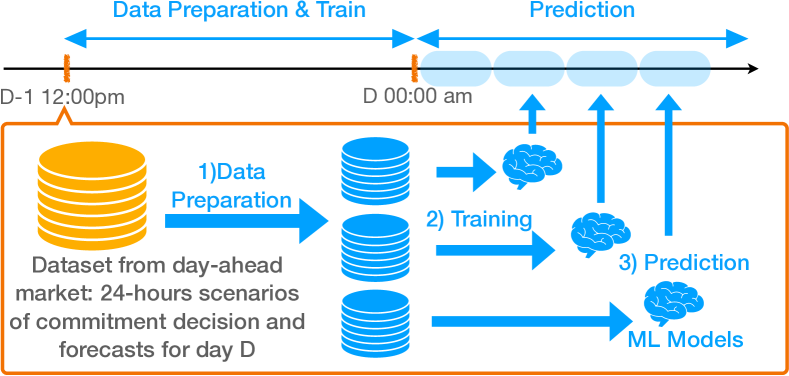
The proposed learning pipeline is depicted in Figure 1. First, commitment decisions and day-ahead forecasts for load and renewable generation are gathered, following the clearing of the day-ahead market. Second, this information is used to generate a training dataset of SCED instances, using classical data augmentation techniques. Third, specialized ML models are trained, ideally one for each hour of the operating day, thereby alleviating the combinatorial explosion of commitment decisions: each ML model only needs to consider one set of commitments and focus on load/renewable scenarios around the forecasts for that hour. Fourth, throughout the operating day, the trained models are used in real time to evaluate a large number of scenarios. The entire data-generation and training procedure is completed in a few hours.
The rest of the paper is organized as follows. Section II describes the interplay between day-ahead and real-time markets in the MISO system, and gives an overview of the real-time SCED for MISO. Section III analyzes the behavior of the real-time market solutions, proposes a combined Classification-Then-Regression architecture, and presents the overall ML pipeline. Numerical experiments on a real-life system are reported in Section IV
II Overview of MISO’s Market-Clearing Pipeline
This section describes the interplay between MISO’s day-ahead and real-time markets; the reader is referred to [21] for a detailed overview of MISO’s energy and reserve markets.
II-A MISO Optimization Pipeline
The day-ahead market consists of two phases, and is executed every day at 10am. First, a day-ahead security-constrained unit commitment (DA-SCUC) is executed: it outputs the commitment and regulation status of each generator for every hour of the following day. Then, a day-ahead SCED is executed to compute day-ahead prices and settle the market. The results of the day-ahead market clearing are then posted online at approximately 1pm, i.e., there is a delay of several hours before the commitment decisions take effect. While MISO may commit additional units during the operating day, through out-of-market reliability studies, in practice, of commitment decisions are decided in the day-ahead market [2]. Accordingly, for simplicity and without loss of generality, this paper assumes that commitment decisions from the DA-SCUC are not modified afterwards.
Then, throughout the operating day, the real-time market is executed every 5 minutes. This real-time SCED (RT-SCED) adjusts the dispatch of every generator in response to variations in load and renewable production, and maximizes economic benefit. Despite its short-time horizon, the RT-SCED must still account for uncertainty in load and renewable production. In the MISO system, this uncertainty mainly stems from the intermittency of wind farms, and from increasing variability in load. The latter is caused, in part, by the growing number of behind-the-meter distributed energy resources (DERs) such as residential storage and rooftop solar. Therefore, operators continuously monitor the state of the power grid, and may take preventive and/or corrective actions to ensure safe and reliable operations.
II-B RT-SCED Formulation
The RT-SCED used by MISO is a DC-based linear programming formulation that co-optimizes energy and reserves [22]. The reader is referred to [23] for the full mathematical formulation; only its core elements are described here. The computation of market-clearing prices is beyond the scope of this paper, and is therefore not discussed here.
The RT-SCED model comprises, for each generator, one variable for energy dispatch and up to four categories of reserves: regulating, spinning, online supplemental, and offline supplemental. In addition, each generator is subject to ramping constraints and individual limits on energy and reserve dispatch. Energy production costs are modeled as piece-wise linear convex functions. Each market participant submits its own production costs and reserve prices via MISO’s market portal, and may submit different offers for each hour of the day. For intermittent generators such as solar and wind, the latest forecast is used in lieu of binding offers.
At the system level, line losses are estimated in real-time from MISO’s state estimator, and incorporated in the formulation using a loss factor approach as in [24]. Transmission constraints are modeled using PTDF matrices, where flow sensitivities with respect to power injections and withdrawals are provided by an external tool. Reserves are dispatched on individual generators, in order to meet zonal and market-wide minimum requirements. Additional constraints ensure that, in a contingency event, reserves may be deployed without tripping transmission lines. Power balance, reserve requirements, and transmission limits are soft, i.e., they may be violated, albeit at a reasonably high cost.
In summary, the RT-SCED receives the following inputs: the commitment decisions from DA-SCUC, the most recent forecast for load and renewable production, the economic limits and production costs of the generators, the current state estimation, and the transmission constraints and reserve requirements. The RT-SCED produces as outputs the active power and reserve dispatch for each generator.
III The Learning Methodology
This section reviews the learning methodology for the RT-SCED. First, Section III-A presents an analysis of the behavior of optimal SCED solutions in MISO’s optimization pipeline. These patterns motivate a novel ML architecture, which is described in Section III-B, followed by an overview of the proposed ML pipeline in Section III-C. Further details on the data are given in Section IV, as wells as in [25].
III-A Pattern Analysis of Optimal SCED solutions
The system at hand is the French transmission system, whose network topology is provided by the French TSO, RTE. It contains buses, transmission lines and transformers, and individual generators, of which are wind and solar generators and are conventional units. The MISO optimization pipeline, described in Section II, is replicated on this system for the entire year 2018, yielding DA-SCUC instances and about RT-SCED instances. Relevant statistics are reported next.
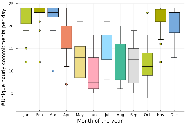
First, unsurprisingly, commitment decisions display a high variability; for example, in 2018, a total of different hourly commitments were recorded across the total hours of the year, where each “hourly commitment” is a binary vector of size 713 that contains the (hourly) commitment status of conventional generators. The intra-day variability of commitment decisions follows a seasonal pattern, which is illustrated in Figure 2. Namely, for each month of the year, Figure 2 displays the distribution, across every day of the month, of the number of unique hourly commitments over a day. The higher values correspond to the higher variability in commitment decisions, while the lower values indicate that the commitment decisions are stable throughout the day. Typically, the variability of commitment decisions is lower in summer and higher in winter; this behavior is expected since more generators are online in winter, which naturally tends to yield more diverse commitments. Indeed, in June 2018, all the days have at least 5 and at most 19 different hourly commitments, with of days having less than 7 and having more than 8. In contrast, in January 2018, except for two outliers, every day has at least 19 different commitments, and 16 days had a different commitment decision every hour. Overall this combinatorial explosion of commitment decisions has an adverse effect on ML models, since it creates distribution shifts on unseen commitments that is detrimental to the performance.
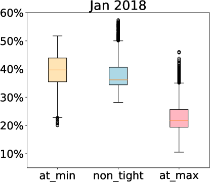
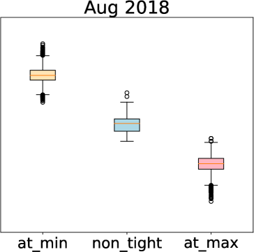
Second, an analysis of RT-SCED solutions reveals, also unsurprisingly, that a majority of generators are dispatched to either their minimum or maximum limit; such limits include economic offer data and ramping constraints. Detailed statistics are reported in Figure 3 for January and August 2018: each plot quantifies, across all RT-SCED instances for that month, the proportion of generators dispatched at their minimum (at_min) or maximum (at_max) limit, or neither (non_tight); these statistics exclude the renewable generators and the generators for which the minimum and maximum limit are identical. In January, the median proportion of generators being dispatched at their minimum (resp., maximum) limit is close to (resp., ), while in August, these values are around and . The variability is also visibly higher in winter, echoing the previous observations for commitment decisions.
III-B First Classify, then Perform Regression
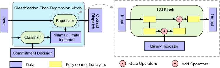
The previous analysis indicates that, given the knowledge of which generators are dispatched to their minimum or maximum limit, only a small number of generators need to be predicted. This suggests a Classification-Then-Regression (CTR) approach, first screening the active generators to identify those at their bounds, and then applying a regression to predict the dispatch of the remaining generators. The overall architecture is depicted in Figure 4. The input of the learning task is a dataset , where , , represent the observation of the system state, the status indicators of the generators (i.e., whether each generator is at its maximum/minimum limits), and the optimal dispatches, respectively.
| Feature | Size | Source |
|---|---|---|
| Loads | Load forecasts | |
| Cost of generators | Bids | |
| Cost of reserves | Bids | |
| Previous solution | SCED | |
| Commitment decisions | SCUC | |
| Reserve Commitments | SCUC | |
| Generator min/max limits | Renewable forecasts | |
| Line losses factor | System |
The CTR model is composed of two modules; classifier and regressor. First, the classifier component aims at classifying whether each generator is at its minimum or maximum limit. It considers the status of the power network with buses, generators, and loads as its inputs. Specifically, the classifier, parameterized by , is a mapping , where is the dimension of the input features. The overall input features describe the state of the power system, detailed in Table I. Also, it outputs the binary vector of meaning that, for each generator, there are two classification choices: one for determining whether it is dispatched at its maximum limit and one for determining whether it is dispatched at its minimum limit. In the experiments presented in the subsequent section, the dimension of the input space can be as large as in the RTE system. The optimal trainable parameters in the classifier are obtained through minimizing the loss function as follows:
| (1) |
where denotes the cross entropy loss, i.e.,
| (2) |
The second architectural component, the regressor that is parameterized by , is a mapping . The additional features in the input of the regressor come from the outputs of the classifier. Given the trained classifier , the optimal trainable parameters of the regressor are obtained by minimizing the loss function over all training instances as
| (3) |
where is the mean absolute error (MAE) loss, i.e., .
The CTR architecture features a deep neural network (DNN). Specifically, it uses a Latent Surgical Intervention (LSI) network [26] as its building block. LSI is a variant of residual neural networks [27] that is augmented by binary interventions. As illustrated in Figure 4, the LSI block exploits, via gate operators, the binary information coming from commitment decisions and the classifier. As mentioned earlier, because the variability in SCED solutions primarily comes from the combinatorial nature of the commitment decisions, it is crucial to design the DNN architecture to use commitment decisions as the input of the model. Thus, the LSI-based CTR model makes it possible to learn the generator dispatch from various commitment decisions, thereby allowing the proposed approach to generalize to the cases where the models are trained over multiple commitment decisions.
III-C Machine Learning Pipeline
The high variability of SCED instances in real operations, in terms of commitment decisions and forecasts of loads and renewable energy sources, makes it extremely challenging to learn the SCED optimization. To mitigate this significant variability, this paper proposes a learning pipeline that closely follows MISO’s optimization pipeline. The machine-learning pipeline is depicted in Figure 1 and consists of three phases: data preparation, training, and prediction.
Data Preparation
At 12pm of day , the TSO outputs the commitment decisions of generators for the next 24 hours and Monte-Carlo scenarios for day . Each scenario consists of 15 minute-level forecasts for load demands and renewable generators. Since the SCED is solved every 5 minutes throughout a day, the ML pipeline first linearly interpolates the forecasts at 5 minute level. Further data augmentation may be performed, if necessary, by perturbing load and renewable generations following the strategy described in [9]. The data is then used as input to SCED optimization models, which generate the various optimal dispatches. The entire dataset is then divided into subsets, each of which spans one or a few hours, based on computational considerations. Indeed, the goal is to strike the proper balance between the accuracy of the models and the training time, since the models have to be available before midnight. This data preparation process yields the input instances to the learning task described previously.
Training
First, each subset is split into the traditional training/validation/test instances. The CTR models are trained on training instances in sequence while the validation dataset is used for hyperparameter tuning and the test dataset is used for reporting the performance of the machine learning models. This training step takes place in parallel for each subset.
Prediction
Starting from midnight on day , at each time step, the corresponding ML model takes the latest system state as input and predicts the optimal dispatch of SCED models in real-time.
IV Experimental Results
IV-A Test Cases
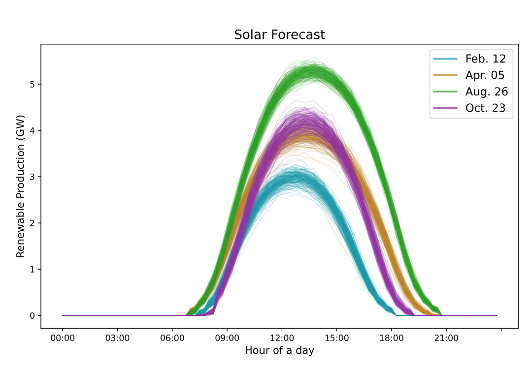
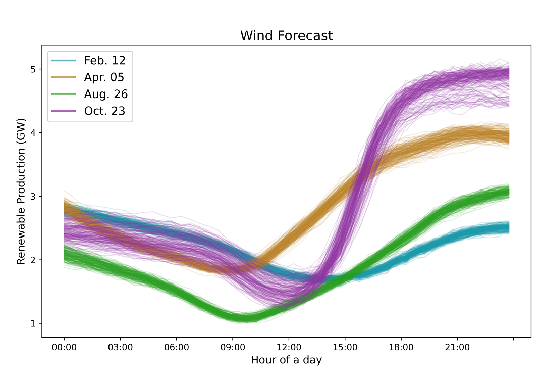
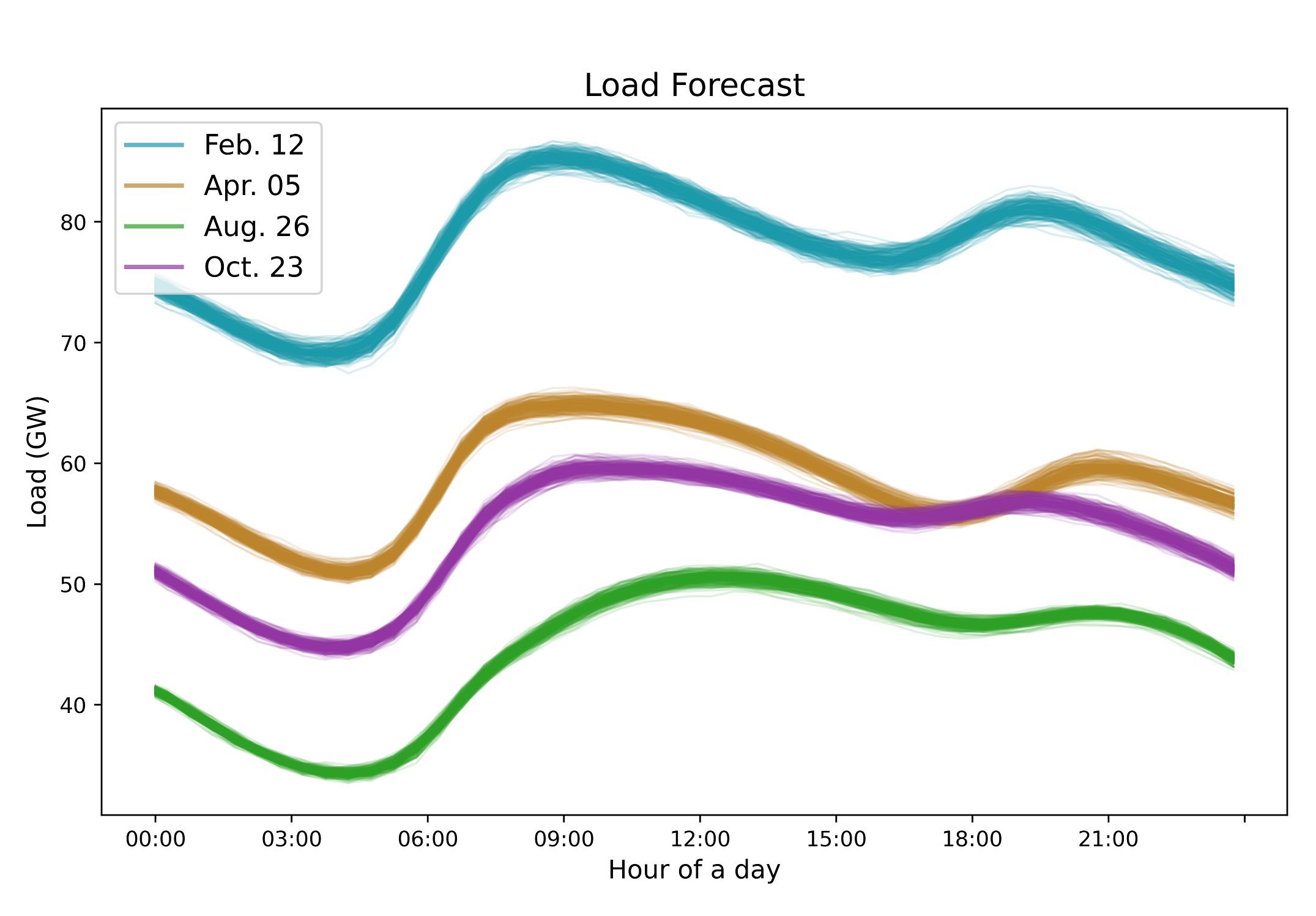
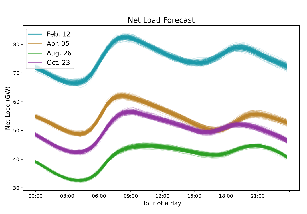
The experiments replicate MISO’s operations on the French transmission system, for four representative days in 2018, namely, February 12th, April 5th, August 26th, and October 23rd. These four days were selected at random to represent annual seasonality. For each operating day, 2000 Monte-Carlo scenarios for total load and renewable power production are sampled in a day-ahead fashion, i.e., scenarios are produced at noon of the previous day. These scenarios are illustrated in Figure 5, which displays 200 scenarios for solar production, wind production, total load, and total net load, respectively. The total net load in this figure represents the amount of power production expected to be generated by the conventional generators, which is identical to the total load minus the renewable generation.
The forecasting models for load consumption and renewable power generation in this paper used Long Short-Term Memory (LSTM) neural networks [28] and the scenarios are generated by a MC-dropout approach [29]. Other forecasting methods and scenario generation approaches could be used instead, without changing the methodology.
Day-ahead commitment decisions are obtained by solving a DA-SCUC problem and recording its solution. The SCUC formulation used in the present experiment follows MISO’s DA-SCUC described in [21, 30]. Again, the proposed ML pipeline is agnostic to the SCUC formulation itself and how it is solved, as it only requires the resulting commitments.
Finally, for each scenario and each day, 288 RT-SCED instances are solved (one every 5 minutes), yielding a total of instances. This initial dataset is then divided into 24 hourly datasets, each containing SCED instances, since commitment decisions are hourly. To avoid information leakage, the data is split between training/validation/testing instances as follows: of scenarios are used for training, for validation, and for testing. All the reported results are in terms of the testing instances.
The optimization problems (SCUC and SCED) are formulated in the JuMP modeling language [31] and solved with Gurobi 9.1 [32], using Linux machines with dual Intel Xeon 6226@2.7GHz CPUs on the PACE Phoenix cluster [33]; the entire data generation phase is performed in less than 2 hours. The proposed CTR model is implemented using PyTorch [34] and trained using the Adam optimizer [35] with a learning rate of 5e-4. A grid search is performed to choose the hyperparameters, i.e., the dimension of the hidden layers (taken in the set {64, 128, 256}), and the number of layers (from the set {2, 3, 4, 5, 6}) for the fully connected layers in the LSI block. A leaky ReLU with leakiness of is used as the activation function in the LSI block. An early stopping criterion with 20 epochs is used for training the classifier and regressor models in order to prevent overfitting: when the loss values (Eq. 1 and Eq. 3) on the validation dataset do not decrease for 20 consecutive epochs, the training process is terminated. Training is performed using Tesla V100-PCIE GPUs with 16GBs HBM2 RAM, on machines with Intel CPU cores at 2.1GHz.
IV-B Baselines
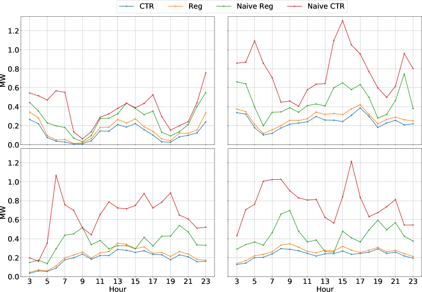
The proposed CTR models are evaluated against the following baselines: Naive CTR, Naive Regression (Naive Reg), and Regression (Reg). The naive baselines replicate the behavior of the previous SCED solution, i.e., they use the dispatch solution obtained 5 minutes earlier. The naive baselines are motivated by the fact that, if the system does not change much between two consecutive intervals, then the SCED solution should not be changed much either. The Naive CTR uses the same approach as the CTR models: it first predicts whether a given generator is at its minimum (resp., maximum) limit if it was at its minimum (resp. maximum) limit in the previous dispatch; then, for the remaining generators, it predicts the active dispatch using the regressor. The naive baselines are expected to perform worse when large fluctuations in load and renewable production are observed, which typically occurs in the morning and evening. Note that these times of the day also display the largest ramping needs, and are among the most critical for reliability. The effectiveness of the CTR architecture is also demonstrated by comparing it to Reg for the optimal active dispatch, i.e., by omitting the classification step from the CTR.
IV-C Optimal Dispatch Prediction Errors
| Dates | |||||
|---|---|---|---|---|---|
| Methods | Feb. 12 | Apr. 5 | Aug. 26 | Oct. 23 | Avg. |
| Naive classifier | 98.26 | 97.79 | 98.64 | 98.31 | 98.25 |
| CTR | 99.56 | 99.18 | 99.40 | 99.24 | 99.35 |
Table II reports the overall classification accuracy of the CTR classifier and the Naive CTR across four representative days in 2018. Surprisingly, the naive classifier is a strong baseline, with an accuracy that ranges from in the Spring to in the Summer. The CTR classifier always improves on the baseline, by around one percentage point on average and by up to percentage point in the Spring. More detailed results about the classifiers are given in Appendix -A.
| Date | Method | Small | Medium | Large | All |
|---|---|---|---|---|---|
| Feb. 12 | Naive Reg | 0.122 | 0.465 | 1.602 | 0.374 |
| Naive CTR | 0.084 | 0.333 | 1.128 | 0.262 | |
| Reg | 0.057 | 0.188 | 0.654 | 0.153 | |
| CTR | 0.043 | 0.141 | 0.535 | 0.117 | |
| Apr. 05 | Naive Reg | 0.242 | 0.345 | 7.480 | 0.772 |
| Naive CTR | 0.197 | 0.220 | 4.374 | 0.463 | |
| Reg | 0.149 | 0.152 | 2.553 | 0.282 | |
| CTR | 0.105 | 0.110 | 2.291 | 0.241 | |
| Aug. 26 | Naive Reg | 0.097 | 0.256 | 7.447 | 0.637 |
| Naive CTR | 0.080 | 0.149 | 4.045 | 0.352 | |
| Reg | 0.054 | 0.124 | 2.454 | 0.218 | |
| CTR | 0.034 | 0.064 | 2.220 | 0.190 | |
| Oct. 23 | Naive Reg | 0.176 | 0.535 | 8.425 | 0.778 |
| Naive CTR | 0.140 | 0.341 | 4.596 | 0.434 | |
| Reg | 0.106 | 0.192 | 2.724 | 0.263 | |
| CTR | 0.076 | 0.145 | 2.525 | 0.235 |
†Small: 0-10MW; Medium: 10-100MW; Large: 100MW
Figure 6 reports the mean absolute error (MAE) for active power dispatch of the different models for each of the considered days. Given a ground-truth dispatch and the predicted dispatch , the MAE is defined as
where is the number of instances in the test dataset and is the number of generators for each instance. As shown in Figure 6, the MAEs of CTR are always lower than those of Reg, demonstrating the benefits of the classifier. The MAEs of Naive CTR are always lower than those of Naive Reg, showing that even a naive classifier has benefits. Moreover, the methods using DNNs for classification and regression, i.e., CTR and Reg, are always better than their naive counterparts, demonstrating the value of deep learning. Note that the performance of the naive methods fluctuates during the day, mainly due to the variability of the commitments. The naive methods are not robust with respect to changes in commitments, contrary to the proposed CTR approach.
To investigate how the machine-learning models perform for different generator types, Table III reports their behavior for different generator sizes. The generators are clustered into three groups based on their actual active dispatches, and the MAE is reported for each group separately. Small-size generators have a capacity between and MW, medium-size generators have a capacity between and MW, and large-size generators have a capacity above MW. The last column report the MAEs across all generators. Table III further confirms that the CTR models consistently outperform the corresponding regressors. These improvements are most notable for small and medium generators which are expected to have higher variability: the MAEs are decreased by up to across small generators and across medium generators (in Aug. 26). Moreover, across four days, the CTR model achieves a Mean Average Percentage Error (MAPE) of and for medium and large generators.
IV-D Solving Time vs Inference Time
Solving the SCED using traditional optimization tools takes, on average, seconds. Actual computing times fluctuate throughout the day, with increased load and congestion leading to higher computing times. In contrast, evaluating the optimization proxy for a batch of 288 instances takes an average milliseconds. In other words, roughly scenarios may be evaluated in less than one second. This represents an improvement of 4 orders of magnitude, even under the assumption that several hundred SCED instances can be solved in parallel.
V Sensitivity Analysis
V-A Motivations and Experiment Settings
How many CTR models need to be trained is an important question to ponder in practice. Preparing a single CTR model for 24 hours on Day would be most convenient. However, as described in Section III-A, the variability in commitments is notoriously harmful to the prediction accuracy and training time of the CTR model. However, successive hours during a day may only have a few differences in commitments and hence a single CTR model may be sufficient for predicting the associated SCED optimizations.
To answer that question, the original instance data is used to produce a variety of datasets, containing data for consecutive 2, 3, 4, 6, 8, 12, and 24 hours. For instance, the 8 hours dataset contains three sets of instances, each grouping SCED data for 8 successive hours. Three models are then trained using instances covering their 8 hours of data. All models use the termination criterion presented in Section IV. The various CTR models for 1, 2, …, 24 hours are then compared for the 24 hours of the day, using the models appropriate for each hour. It is expected that the quality of the prediction will deteriorate with a coarser granularity, since there will be a larger variability in commitments and net loads. However, the LSI architecture of the CTR model and the availability of more instances during training may compensate for this increase in variability. In the following, CTR models trained on hours are denoted as CTRi.
V-B Results
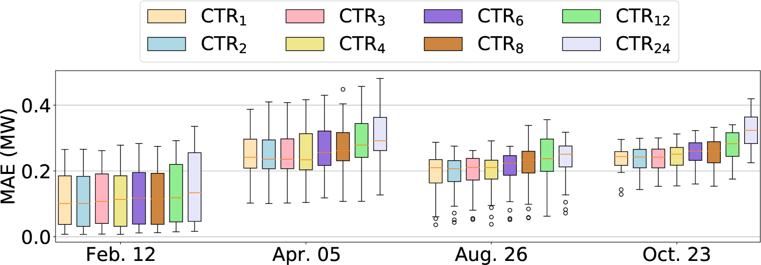
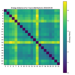
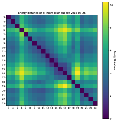
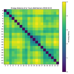
Figure 7 illustrates the MAE values of the various CTR models. The performance of the CTR model remains strong even when aggregating up to 4 successive hours. As more hours are aggregated, the performance starts to degrade. To get more insight on the performance of the various CTR models, it is useful to consider the energy distance [36] between the empirical distributions of the testing and training instances. Recall that, given two empirical distributions and , their energy distance is given by
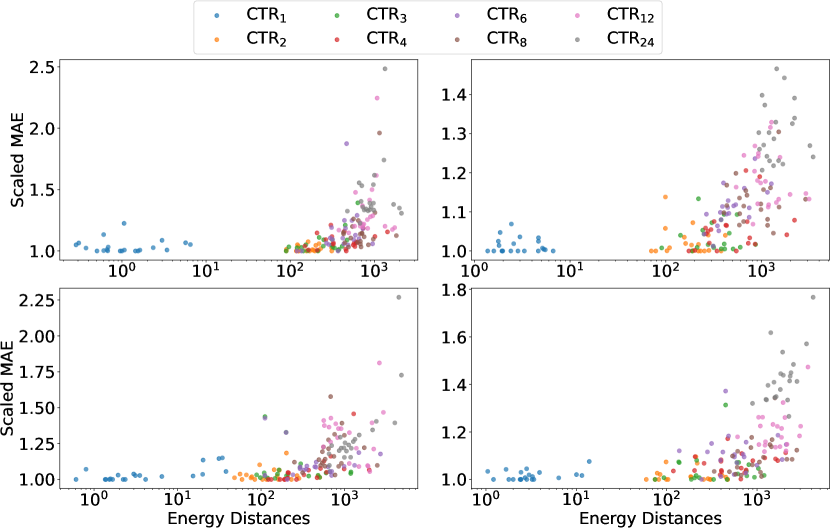
It is thus interesting to study the relationship between the MAE of a CTR model and the energy distance between its testing and training datasets. Figure 8 reports the relationship between the scaled MAE and the energy distance, where the scaled MAE is the MAE value divided by the best MAE value across all experiments. Each dot captures the scaled MAE value (y-axis) for a CTR model and the associated energy distance (x-axis) between its training and testing datasets.
Observe first that the energy distance increases as more hourly data are combined into the training set. In Figure 8, the dots from CTRi tend to have smaller energy distances than those of CTRj for . The scaled MAE also increases as the energy distance grows. More interestingly, Figure 8 shows that the MAE value only increases slightly as the energy distance becomes larger. Specifically, an increase of in energy distance produces an increase of only 10% in MAE (corresponding to a scaled MAE of 1.1). These results confirm that the CTR models scale well when facing a reasonable amount of variability in commitment decisions and net loads. However, when the energy distance goes over a certain threshold, then the performance of CTR models starts to degrade significantly even in presence of more data and more training time. Note that the energy distance between the training and testing datasets can be computed before the training process. Hence, the proper granularity for the CTR model can be chosen to obtain the desired accuracy. This quantification shows the potential of CTR to perform well with more complex components involved in the MISO pipeline such as the Look Ahead Commitment (LAC).
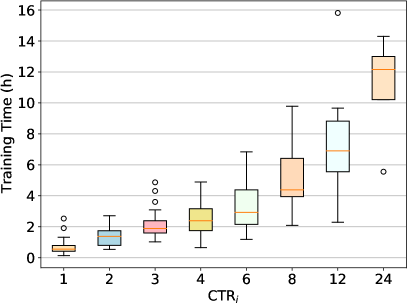
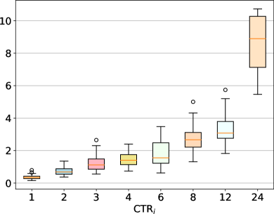
Figure 9 reports the training times of the CTR models. The average training time increases as more hourly data are included. The regression takes more training time than the classification task. Section III-C indicated that the training process must complete within about 12 hours after accumulating the data instances at 12pm on day . This is clearly possible for all the CTRi models with . Consider CTR4 for instance. Figure 9 shows that it can be trained for a 4-hour block within 10 hours in the worst case (4 hours for classification and 6 hours for regression). As a result, all 6 CRT4 models can easily be trained in parallel within the required time frame.
VI Conclusion
The paper presented several challenges that may hamper the use of ML models in power systems operations, including the variability of electricity demand and renewable production, the variations in production costs, and the combinatorial structure of commitment decisions. To address these challenges, the paper proposed a novel ML pipeline that leverages day-ahead forecasts and the TSO’s knowledge of commitment decisions several hours before they take place. The proposed pipeline consists of two main phases: 1) day-ahead data preparation and training; and 2) real-time predictions, which fits naturally within the operations of a TSO. Moreover, informed by the behavior of real-time markets, the paper proposed a novel Classification-Then-Regression (CTR) approach that leverages deep neural networks based on Latent Surgical Interventions to capture generator commitments and generators operating at their limits. Computational experiments that replicated MISO’s operational pipeline on a real, large-scale transmission system demonstrated the feasibility of the approach. In particular, the results show that optimization proxies based on ML models have the potential to provide operators with new tools for real-time risk monitoring.
Several extensions are possible, which will be the topic of future work. The integration, during training, of Lagrangian-based penalties has the potential to further improve the performance of the neural network models. Such methods have been shown to improve the feasibility of the predictions with respect to the original constraints. Moreover, once trained, the proposed classifier may be used to also accelerate the SCED resolution, by providing hints as to which variables should be fixed at their minimum or maximum limit. Finally, the proposed CTR model is not limited to SCED models, and may be applied to any optimization problems.
Acknowledgments
This research is partly funded by NSF Awards 1912244 and 2112533, and ARPA-E Perform Award AR0001136.
References
- [1] A. J. Conejo and L. Baringo, Power system operations. Springer, 2018.
- [2] Y. Chen, F. Wang, J. Wan, and F. Pan, “Developing next generation electricity market clearing optimization software,” in 2018 IEEE Power Energy Society General Meeting (PESGM), 2018, pp. 1–5.
- [3] N. Chiang and A. Grothey, “Solving security constrained optimal power flow problems by a structure exploiting interior point method,” Optimization and Engineering, vol. 16, no. 1, pp. 49–71, 2015.
- [4] Q. Wang, J. D. McCalley, T. Zheng, and E. Litvinov, “Solving corrective risk-based security-constrained optimal power flow with Lagrangian relaxation and Benders decomposition,” International Journal of Electrical Power & Energy Systems, vol. 75, pp. 255–264, 2016.
- [5] A. Velloso, P. Van Hentenryck, and E. S. Johnson, “An exact and scalable problem decomposition for security-constrained optimal power flow,” Electric Power Systems Research, vol. 195, p. 106677, 2021.
- [6] T. Werho, J. Zhang, V. Vittal, Y. Chen, A. Thatte, and L. Zhao, “Scenario generation of wind farm power for real-time system operation,” 2021.
- [7] X. Pan, T. Zhao, and M. Chen, “Deepopf: Deep neural network for dc optimal power flow,” in 2019 IEEE International Conference on Communications, Control, and Computing Technologies for Smart Grids (SmartGridComm). IEEE, 2019, pp. 1–6.
- [8] F. Fioretto, T. W. Mak, and P. Van Hentenryck, “Predicting ac optimal power flows: Combining deep learning and lagrangian dual methods,” in Proceedings of the AAAI Conference on Artificial Intelligence, vol. 34, no. 01, 2020, pp. 630–637.
- [9] M. Chatzos, F. Fioretto, T. W. Mak, and P. Van Hentenryck, “High-fidelity machine learning approximations of large-scale optimal power flow,” arXiv preprint arXiv:2006.16356, 2020.
- [10] X. Lei, Z. Yang, J. Yu, J. Zhao, Q. Gao, and H. Yu, “Data-driven optimal power flow: A physics-informed machine learning approach,” IEEE Transactions on Power Systems, vol. 36, no. 1, pp. 346–354, 2020.
- [11] M. Chatzos, T. W. Mak, and P. Van Hentenryck, “Spatial network decomposition for fast and scalable ac-opf learning,” arXiv preprint arXiv:2101.06768, 2021.
- [12] A. Velloso and P. Van Hentenryck, “Combining deep learning and optimization for security-constrained optimal power flow,” arXiv preprint arXiv:2007.07002, 2020.
- [13] A. S. Zamzam and K. Baker, “Learning optimal solutions for extremely fast ac optimal power flow,” in 2020 IEEE International Conference on Communications, Control, and Computing Technologies for Smart Grids (SmartGridComm). IEEE, 2020, pp. 1–6.
- [14] D. Owerko, F. Gama, and A. Ribeiro, “Optimal power flow using graph neural networks,” in ICASSP 2020-2020 IEEE International Conference on Acoustics, Speech and Signal Processing (ICASSP). IEEE, 2020, pp. 5930–5934.
- [15] D. Deka and S. Misra, “Learning for dc-opf: Classifying active sets using neural nets,” in 2019 IEEE Milan PowerTech. IEEE, 2019, pp. 1–6.
- [16] S. Misra, L. Roald, and Y. Ng, “Learning for constrained optimization: Identifying optimal active constraint sets,” INFORMS Journal on Computing, 2021.
- [17] Á. S. Xavier, F. Qiu, and S. Ahmed, “Learning to solve large-scale security-constrained unit commitment problems,” INFORMS Journal on Computing, vol. 33, no. 2, pp. 739–756, 2021.
- [18] Y. Yang, Z. Yang, J. Yu, K. Xie, and L. Jin, “Fast economic dispatch in smart grids using deep learning: An active constraint screening approach,” IEEE Internet of Things Journal, vol. 7, no. 11, pp. 11 030–11 040, 2020.
- [19] N. Guha, Z. Wang, M. Wytock, and A. Majumdar, “Machine learning for ac optimal power flow,” arXiv preprint arXiv:1910.08842, 2019.
- [20] A. Venzke, D. T. Viola, J. Mermet-Guyennet, G. S. Misyris, and S. Chatzivasileiadis, “Neural networks for encoding dynamic security-constrained optimal power flow to mixed-integer linear programs,” arXiv preprint arXiv:2003.07939, 2020.
- [21] MISO, “Energy and operating reserve markets,” Business Practices Manual Energy and Operating Reserve Markets.
- [22] X. Ma, Y. Chen, and J. Wan, “Midwest iso co-optimization based real-time dispatch and pricing of energy and ancillary services,” in 2009 IEEE Power Energy Society General Meeting, 2009, pp. 1–6.
- [23] MISO, “Real-time energy and operating reserve market software formulations and business logic,” Business Practices Manual Energy and Operating Reserve Markets Attachment D.
- [24] B. Eldridge, R. P. O’Neill, and A. Castillo, “Marginal loss calculations for the dcopf,” 2017.
- [25] M. Chatzos, M. Tanneau, and P. Van Hentenryck, “Data-driven Time Series Reconstruction for Modern Power Systems Research,” submitted.
- [26] B. Donnot, I. Guyon, Z. Liu, M. Schoenauer, A. Marot, and P. Panciatici, “Latent surgical interventions in residual neural networks,” 2018.
- [27] K. He, X. Zhang, S. Ren, and J. Sun, “Identity mappings in deep residual networks,” in European conference on computer vision. Springer, 2016, pp. 630–645.
- [28] S. Hochreiter and J. Schmidhuber, “Long short-term memory,” Neural computation, vol. 9, no. 8, pp. 1735–1780, 1997.
- [29] Y. Gal and Z. Ghahramani, “Dropout as a bayesian approximation: Representing model uncertainty in deep learning,” in international conference on machine learning. PMLR, 2016, pp. 1050–1059.
- [30] MISO, “Day-ahead energy and operating reserve market software formulations and business logic,” Business Practices Manual Energy and Operating Reserve Markets Attachment B.
- [31] I. Dunning, J. Huchette, and M. Lubin, “Jump: A modeling language for mathematical optimization,” SIAM Review, vol. 59, no. 2, pp. 295–320, 2017.
- [32] Gurobi Optimization, LLC, “Gurobi Optimizer Reference Manual,” 2021. [Online]. Available: https://www.gurobi.com
- [33] PACE, Partnership for an Advanced Computing Environment (PACE), 2017. [Online]. Available: http://www.pace.gatech.edu
- [34] A. Paszke, S. Gross, F. Massa, A. Lerer, J. Bradbury, G. Chanan, T. Killeen, Z. Lin, N. Gimelshein, L. Antiga, A. Desmaison, A. Kopf, E. Yang, Z. DeVito, M. Raison, A. Tejani, S. Chilamkurthy, B. Steiner, L. Fang, J. Bai, and S. Chintala, “Pytorch: An imperative style, high-performance deep learning library,” in Advances in Neural Information Processing Systems 32, H. Wallach, H. Larochelle, A. Beygelzimer, F. d'Alché-Buc, E. Fox, and R. Garnett, Eds. Curran Associates, Inc., 2019, pp. 8024–8035.
- [35] D. P. Kingma and J. Ba, “Adam: A method for stochastic optimization,” arXiv preprint arXiv:1412.6980, 2014.
- [36] M. L. Rizzo and G. J. Székely, “Energy distance,” wiley interdisciplinary reviews: Computational statistics, vol. 8, no. 1, pp. 27–38, 2016.
-A Classification accuracy across four days
The detailed results of Naive and CTR model trained under different hourly data in four days are shown in Table IV V VI VII, respectively. First, across all days, CTR models always outperform the baseline model. Moreover, the performance decay is up to for Naive model (in Apr. 5) and up to for CTR model (CTR12 in Aug. 26) along the day. CTR models have much smaller performance variations with the fluctuation of loads and renewables along the four days. Second, the CTR model scales well with more hours data included. The stark performance decay can only be observed with more than 12 hours data included.
| Hour | Naive | CTR1 | CTR2 | CTR3 | CTR4 | CTR6 | CTR8 | CTR12 | CTR24 |
|---|---|---|---|---|---|---|---|---|---|
| 03:00 - 04:00 | 98.37 | 99.24 | 99.24 | 99.29 | 99.24 | 99.31 | 99.26 | 99.17 | 98.94 |
| 04:00 - 05:00 | 98.79 | 99.36 | 99.38 | 99.40 | 99.32 | 99.42 | 99.37 | 99.30 | 99.11 |
| 05:00 - 06:00 | 98.74 | 99.68 | 99.70 | 99.71 | 99.69 | 99.71 | 99.70 | 99.65 | 99.55 |
| 06:00 - 07:00 | 98.60 | 99.85 | 99.87 | 99.86 | 99.87 | 99.86 | 99.86 | 99.84 | 99.77 |
| 07:00 - 08:00 | 98.14 | 99.88 | 99.88 | 99.87 | 99.85 | 99.87 | 99.85 | 99.85 | 99.80 |
| 08:00 - 09:00 | 98.66 | 99.97 | 99.97 | 99.97 | 99.97 | 99.97 | 99.96 | 99.96 | 99.95 |
| 09:00 - 10:00 | 99.27 | 99.96 | 99.96 | 99.96 | 99.97 | 99.96 | 99.96 | 99.95 | 99.94 |
| 10:00 - 11:00 | 99.04 | 99.80 | 99.80 | 99.80 | 99.79 | 99.77 | 99.77 | 99.74 | 99.70 |
| 11:00 - 12:00 | 97.64 | 99.24 | 99.38 | 99.38 | 99.34 | 99.29 | 99.31 | 99.21 | 99.08 |
| 12:00 - 13:00 | 97.96 | 99.37 | 99.36 | 99.34 | 99.31 | 99.30 | 99.31 | 99.19 | 99.04 |
| 13:00 - 14:00 | 97.97 | 99.22 | 99.26 | 99.25 | 99.21 | 99.21 | 99.18 | 99.05 | 98.91 |
| 14:00 - 15:00 | 97.25 | 99.29 | 99.32 | 99.30 | 99.29 | 99.29 | 99.27 | 99.13 | 98.95 |
| 15:00 - 16:00 | 98.37 | 99.25 | 99.23 | 99.25 | 99.18 | 99.19 | 99.16 | 99.06 | 98.94 |
| 16:00 - 17:00 | 98.71 | 99.52 | 99.53 | 99.54 | 99.53 | 99.51 | 99.45 | 99.43 | 99.34 |
| 17:00 - 18:00 | 98.12 | 99.69 | 99.69 | 99.68 | 99.69 | 99.65 | 99.62 | 99.59 | 99.53 |
| 18:00 - 19:00 | 98.93 | 99.88 | 99.88 | 99.88 | 99.88 | 99.82 | 99.83 | 99.82 | 99.78 |
| 19:00 - 20:00 | 99.17 | 99.87 | 99.88 | 99.88 | 99.88 | 99.84 | 99.85 | 99.83 | 99.81 |
| 20:00 - 21:00 | 99.03 | 99.68 | 99.64 | 99.69 | 99.59 | 99.58 | 99.59 | 99.58 | 99.54 |
| 21:00 - 22:00 | 97.83 | 99.47 | 99.47 | 99.39 | 99.38 | 99.31 | 99.38 | 99.33 | 99.22 |
| 22:00 - 23:00 | 96.11 | 99.45 | 99.47 | 99.42 | 99.37 | 99.32 | 99.36 | 99.30 | 99.23 |
| 23:00 - 24:00 | 96.82 | 99.02 | 98.96 | 98.89 | 98.82 | 98.76 | 98.81 | 98.71 | 98.60 |
| Hour | Naive | CTR1 | CTR2 | CTR3 | CTR4 | CTR6 | CTR8 | CTR12 | CTR24 |
|---|---|---|---|---|---|---|---|---|---|
| 03:00 - 04:00 | 97.95 | 99.24 | 99.24 | 99.24 | 99.24 | 99.24 | 99.21 | 99.11 | 98.95 |
| 04:00 - 05:00 | 98.29 | 99.34 | 99.33 | 99.33 | 99.31 | 99.33 | 99.31 | 99.23 | 99.08 |
| 05:00 - 06:00 | 98.43 | 99.44 | 99.45 | 99.46 | 99.44 | 99.46 | 99.44 | 99.36 | 99.19 |
| 06:00 - 07:00 | 99.02 | 99.66 | 99.69 | 99.69 | 99.69 | 99.60 | 99.69 | 99.65 | 99.55 |
| 07:00 - 08:00 | 98.20 | 99.56 | 99.54 | 99.55 | 99.53 | 99.46 | 99.53 | 99.49 | 99.35 |
| 08:00 - 09:00 | 98.22 | 99.31 | 99.34 | 99.30 | 99.32 | 99.24 | 99.23 | 99.24 | 99.11 |
| 09:00 - 10:00 | 98.05 | 99.27 | 99.27 | 99.27 | 99.28 | 99.15 | 99.16 | 99.17 | 98.97 |
| 10:00 - 11:00 | 98.40 | 99.26 | 99.29 | 99.30 | 99.30 | 99.21 | 99.23 | 99.23 | 99.08 |
| 11:00 - 12:00 | 97.68 | 98.94 | 98.97 | 98.98 | 99.00 | 98.86 | 98.89 | 98.88 | 98.64 |
| 12:00 - 13:00 | 97.11 | 98.46 | 98.51 | 98.45 | 98.44 | 98.22 | 98.42 | 98.10 | 98.05 |
| 13:00 - 14:00 | 97.36 | 98.83 | 98.80 | 98.77 | 98.78 | 98.56 | 98.65 | 98.45 | 98.32 |
| 14:00 - 15:00 | 96.64 | 98.94 | 98.97 | 98.98 | 99.00 | 98.82 | 98.89 | 98.71 | 98.64 |
| 15:00 - 16:00 | 96.55 | 99.10 | 99.21 | 99.14 | 99.21 | 99.01 | 99.07 | 98.93 | 98.81 |
| 16:00 - 17:00 | 97.36 | 98.93 | 98.71 | 98.81 | 98.56 | 98.60 | 98.54 | 98.52 | 98.38 |
| 17:00 - 18:00 | 97.03 | 98.72 | 98.59 | 98.67 | 98.51 | 98.46 | 98.47 | 98.42 | 98.31 |
| 18:00 - 19:00 | 98.01 | 99.15 | 99.19 | 99.19 | 99.02 | 99.11 | 99.02 | 98.95 | 98.88 |
| 19:00 - 20:00 | 98.72 | 99.33 | 99.39 | 99.40 | 99.21 | 99.33 | 99.27 | 99.20 | 99.15 |
| 20:00 - 21:00 | 98.87 | 99.37 | 99.41 | 99.42 | 99.38 | 99.38 | 99.31 | 99.24 | 99.21 |
| 21:00 - 22:00 | 98.04 | 99.41 | 99.43 | 99.34 | 99.39 | 99.35 | 99.30 | 99.26 | 99.22 |
| 22:00 - 23:00 | 95.28 | 99.22 | 99.23 | 99.23 | 99.25 | 99.17 | 99.07 | 99.00 | 98.87 |
| 23:00 - 24:00 | 98.37 | 99.39 | 99.36 | 99.35 | 99.37 | 99.33 | 99.25 | 99.22 | 99.16 |
| Hour | Naive | CTR1 | CTR2 | CTR3 | CTR4 | CTR6 | CTR8 | CTR12 | CTR24 |
|---|---|---|---|---|---|---|---|---|---|
| 03:00 - 04:00 | 99.73 | 99.95 | 99.94 | 99.92 | 99.95 | 99.92 | 99.91 | 99.90 | 99.88 |
| 04:00 - 05:00 | 99.73 | 99.92 | 99.91 | 99.89 | 99.88 | 99.89 | 99.88 | 99.88 | 99.85 |
| 05:00 - 06:00 | 99.66 | 99.88 | 99.90 | 99.88 | 99.87 | 99.88 | 99.87 | 99.86 | 99.84 |
| 06:00 - 07:00 | 97.93 | 99.65 | 99.67 | 99.66 | 99.67 | 99.62 | 99.65 | 99.61 | 99.50 |
| 07:00 - 08:00 | 98.94 | 99.63 | 99.63 | 99.63 | 99.63 | 99.60 | 99.60 | 99.59 | 99.51 |
| 08:00 - 09:00 | 98.94 | 99.62 | 99.62 | 99.62 | 99.59 | 99.58 | 99.46 | 99.58 | 99.49 |
| 09:00 - 10:00 | 98.87 | 99.52 | 99.55 | 99.49 | 99.52 | 99.51 | 99.39 | 99.52 | 99.41 |
| 10:00 - 11:00 | 98.91 | 99.59 | 99.58 | 99.57 | 99.58 | 99.57 | 99.50 | 99.58 | 99.50 |
| 11:00 - 12:00 | 97.98 | 99.15 | 99.18 | 99.19 | 99.19 | 99.17 | 99.15 | 99.15 | 99.10 |
| 12:00 - 13:00 | 98.08 | 99.03 | 99.07 | 99.06 | 99.07 | 98.95 | 98.83 | 98.44 | 98.82 |
| 13:00 - 14:00 | 98.31 | 98.71 | 98.87 | 98.97 | 98.98 | 98.81 | 98.64 | 98.35 | 98.65 |
| 14:00 - 15:00 | 98.05 | 98.68 | 98.84 | 98.93 | 98.97 | 98.90 | 98.56 | 98.20 | 98.60 |
| 15:00 - 16:00 | 98.15 | 98.77 | 98.90 | 98.89 | 98.98 | 98.90 | 98.67 | 98.29 | 98.68 |
| 16:00 - 17:00 | 97.85 | 98.75 | 98.75 | 98.88 | 98.62 | 98.94 | 98.32 | 98.19 | 98.66 |
| 17:00 - 18:00 | 98.96 | 99.32 | 99.36 | 99.38 | 99.38 | 99.31 | 99.37 | 99.11 | 99.31 |
| 18:00 - 19:00 | 98.77 | 99.42 | 99.46 | 99.44 | 99.43 | 99.36 | 99.39 | 99.10 | 99.28 |
| 19:00 - 20:00 | 98.68 | 99.64 | 99.64 | 99.63 | 99.61 | 99.59 | 99.58 | 99.42 | 99.53 |
| 20:00 - 21:00 | 98.42 | 99.55 | 99.50 | 99.50 | 99.53 | 99.46 | 99.46 | 99.25 | 99.38 |
| 21:00 - 22:00 | 97.96 | 99.46 | 99.44 | 99.45 | 99.47 | 99.35 | 99.36 | 99.06 | 99.25 |
| 22:00 - 23:00 | 98.63 | 99.59 | 99.61 | 99.59 | 99.62 | 99.52 | 99.53 | 99.31 | 99.46 |
| 23:00 - 24:00 | 98.89 | 99.63 | 99.64 | 99.61 | 99.62 | 99.52 | 99.54 | 99.29 | 99.46 |
| Hour | Naive | CTR1 | CTR2 | CTR3 | CTR4 | CTR6 | CTR8 | CTR12 | CTR24 |
|---|---|---|---|---|---|---|---|---|---|
| 03:00 - 04:00 | 99.46 | 99.75 | 99.75 | 99.71 | 99.75 | 99.70 | 99.71 | 99.64 | 99.60 |
| 04:00 - 05:00 | 98.62 | 99.55 | 99.56 | 99.50 | 99.54 | 99.50 | 99.54 | 99.39 | 99.22 |
| 05:00 - 06:00 | 98.95 | 99.57 | 99.60 | 99.55 | 99.58 | 99.55 | 99.60 | 99.50 | 99.32 |
| 06:00 - 07:00 | 99.16 | 99.55 | 99.56 | 99.53 | 99.55 | 99.42 | 99.55 | 99.42 | 99.29 |
| 07:00 - 08:00 | 98.43 | 99.31 | 99.34 | 99.30 | 99.25 | 99.09 | 99.27 | 99.01 | 98.74 |
| 08:00 - 09:00 | 97.02 | 98.99 | 98.99 | 99.01 | 98.90 | 98.80 | 98.70 | 98.67 | 98.41 |
| 09:00 - 10:00 | 97.14 | 99.03 | 99.05 | 98.90 | 98.91 | 98.83 | 98.71 | 98.65 | 98.33 |
| 10:00 - 11:00 | 97.66 | 98.85 | 98.67 | 98.75 | 98.77 | 98.67 | 98.55 | 98.50 | 98.15 |
| 11:00 - 12:00 | 97.74 | 98.75 | 98.62 | 98.71 | 98.68 | 98.65 | 98.60 | 98.48 | 98.24 |
| 12:00 - 13:00 | 97.34 | 98.61 | 98.70 | 98.65 | 98.52 | 98.41 | 98.51 | 98.26 | 98.05 |
| 13:00 - 14:00 | 98.43 | 98.81 | 98.84 | 98.86 | 98.71 | 98.68 | 98.66 | 98.55 | 98.40 |
| 14:00 - 15:00 | 98.33 | 98.76 | 98.86 | 98.82 | 98.70 | 98.62 | 98.63 | 98.52 | 98.35 |
| 15:00 - 16:00 | 97.00 | 98.64 | 98.83 | 98.76 | 98.63 | 98.57 | 98.52 | 98.33 | 98.07 |
| 16:00 - 17:00 | 98.47 | 99.31 | 99.33 | 99.36 | 99.31 | 99.15 | 99.28 | 99.08 | 98.99 |
| 17:00 - 18:00 | 99.13 | 99.47 | 99.47 | 99.47 | 99.47 | 99.33 | 99.46 | 99.32 | 99.25 |
| 18:00 - 19:00 | 99.13 | 99.57 | 99.58 | 99.57 | 99.54 | 99.55 | 99.54 | 99.43 | 99.36 |
| 19:00 - 20:00 | 98.20 | 99.35 | 99.42 | 99.42 | 99.34 | 99.38 | 99.36 | 99.21 | 99.06 |
| 20:00 - 21:00 | 98.78 | 99.48 | 99.51 | 99.52 | 99.47 | 99.49 | 99.47 | 99.34 | 99.20 |
| 21:00 - 22:00 | 97.76 | 99.54 | 99.53 | 99.52 | 99.52 | 99.52 | 99.50 | 99.40 | 99.18 |
| 22:00 - 23:00 | 98.69 | 99.59 | 99.59 | 99.58 | 99.58 | 99.57 | 99.56 | 99.46 | 99.40 |
| 23:00 - 24:00 | 99.01 | 99.57 | 99.58 | 99.55 | 99.55 | 99.53 | 99.53 | 99.43 | 99.34 |
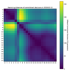
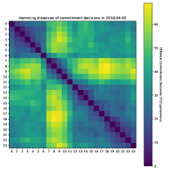
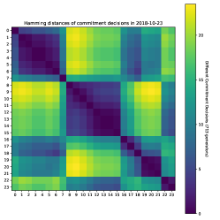
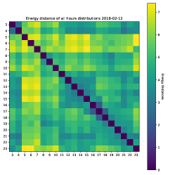
-B Hourly data distribution
The distribution shifts between different hours are measured using the hamming distance of commitment decisions and the energy distance of the input features, shown in Figure 10 and 11, respectively. Each entry indicates the distance between the corresponding hours. Therefore, the diagonal entries are always 0 since the distances between the same dataset are . Interestingly, the block-wise patterns can be observed for energy distances, which is more obvious for hamming distances. Within the block which consists of several consecutive hours, the distribution shift tends to be small. Cross the block, the distribution shift largely. This, to some degree, explains why the CTR models scale well when the span of the combined dataset is less than certain hours, from the data distribution perspective.