TOI 560 : Two Transiting Planets Orbiting a K Dwarf Validated with iSHELL, PFS and HIRES RVs
Abstract
We validate the presence of a two-planet system orbiting the 0.15–1.4 Gyr K4 dwarf TOI 560 (HD 73583). The system consists of an inner moderately eccentric transiting mini-Neptune (TOI 560 b, days, , ) initially discovered in the Sector 8 TESS mission observations, and a transiting mini-Neptune (TOI 560 c, days, ) discovered in the Sector 34 observations, in a rare near-1:3 orbital resonance. We utilize photometric data from TESS Spitzer, and ground-based follow-up observations to confirm the ephemerides and period of the transiting planets, vet false positive scenarios, and detect the photo-eccentric effect for TOI 560 b. We obtain follow-up spectroscopy and corresponding precise radial velocities (RVs) with the iSHELL spectrograph at the NASA Infrared Telescope Facility and the HIRES Spectrograph at Keck Observatory to validate the planetary nature of these signals, which we combine with published PFS RVs from Magellan Observatory. We detect the masses of both planets at significance. We apply a Gaussian process (GP) model to the TESS light curves to place priors on a chromatic radial velocity GP model to constrain the stellar activity of the TOI 560 host star, and confirm a strong wavelength dependence for the stellar activity demonstrating the ability of NIR RVs in mitigating stellar activity for young K dwarfs. TOI 560 is a nearby moderately young multi-planet system with two planets suitable for atmospheric characterization with James Webb Space Telescope (JWST) and other upcoming missions. In particular, it will undergo six transit pairs separated by 6 hours before June 2027.
1 Introduction
The Kepler mission, after its launch in 2009, discovered over 4000 transiting exoplanet candidates (Borucki et al., 2011; Howard et al., 2012; Bryson et al., 2021). However, many of these planets orbited relatively faint 14th-16th visual magnitude stars that were difficult to follow-up, validate and confirm (Plavchan et al., 2015a; Weiss & Marcy, 2014; Wolfgang et al., 2016a; Rogers, 2015; Marcy et al., 2014). The NASA Transiting Exoplanet Survey Satellite (TESS) mission launched in 2018 to detect and identify relatively nearby and brighter transiting exoplanets, particularly those orbiting smaller and cooler M dwarf stars which are the most abundant spectral type, and are known to host compact multi-planet systems (Ricker et al., 2015; Dressing & Charbonneau, 2015; Howard et al., 2012). To date, the TESS mission has expanded the pool of nearby, bright transiting exoplanet candidates considerably, with over 4,000 candidates identified. Many are amenable to ground-based follow-up and characterization (Ricker et al., 2015).
Kepler has shown that compact multi-planet Neptune and terrestrial planets are more commonly found to orbit M dwarf stars (Dressing & Charbonneau, 2015; Howard et al., 2012). Additionally, the relatively small size of M dwarfs in comparison to transiting exoplanets leads to larger, easier-to-detect transit depths, and M dwarfs are the most common spectral types in the Milky Way (Chabrier, 2003; Henry et al., 2006). The relatively nearby M dwarf exoplanet discoveries from TESS are therefore some of the most suitable targets for exoplanet atmospheric characterization with ground-based and future space-based facilities such as JWST (Kempton et al., 2018). Before jumping to atmospheric characterization, however, the TESS candidates need further supporting observations to validate and confirm that they are not false-positives. TESS pixels are in size on the sky, a relatively large value compared to typical ground-based seeing-limited angular resolution of 1”, a design choice for the TESS mission to optimize its cameras’ fields of view (Ricker et al., 2015). As a result, the light from nearby main sequence stars can be blended with fainter visual eclipsing binaries, and produce false-positives, especially when only a singly transiting planet is identified in a 27-day TESS sector of observations at lower ecliptic latitudes away from the ecliptic poles (Ricker et al., 2015; Cale et al., 2021; Vanderburg et al., 2019a; Rodríguez Martínez et al., 2020; Hobson et al., 2021; Addison et al., 2021a; Osborn et al., 2021; Dreizler et al., 2020; Brahm et al., 2020; Nowak et al., 2020; Teske et al., 2020; Sha et al., 2021; Gan et al., 2021; Bluhm et al., 2020).
Ground-based panchromatic light curves, high-resolution imaging with high contrasts, and spectroscopic follow-up can search for close visual companions to the candidate host star to validate that the target is not a false positive from a nearby, background, blended, or grazing eclipsing binary, and to ensure that the planetary radius is unbiased by additional flux sources within the TESS aperture. Additional light curve analyses such as EDI-Vetter Unplugged (Zink et al., 2020) can check for neighboring flux contamination from nearby stars in the sky, examine the abundance of outliers from the transit model, and consider any signal variations between even and odd transits and the presence of any secondary eclipses. The Discovery and Vetting of Exoplanets (DAVE, Kostov et al., 2019) tool evaluates TESS light curve-based diagnostics such as photocenter motion, odd-even transit-depth consistency, searches for secondary eclipses, and other sources of likely false-positive scenarios.
Constraining and/or measuring the masses of transiting planets with precise radial velocities (RVs) derived from high-resolution spectroscopy further enables validation and confirmation of exoplanet candidates, while also providing constraints on the planet bulk densities (Seager et al., 2007; Rogers & Seager, 2010; Zeng et al., 2019). However, RV analysis can be complicated from stellar photospheric activity from young and/or active host stars that can produce RV signals comparable in amplitude of the Keplerian signals of interest. Stellar surface inhomogeneities (e.g., cool spots, hot plages) driven by the dynamic stellar magnetic field rotate in and out of view, leading to photometric variations over time. The presence of such active regions breaks the symmetry between the approaching and receding limbs of the star, introducing apparent RV variations over time as well (Desort et al., 2007). These active regions further affect the integrated convective blue-shift over the stellar disk, and will therefore manifest as an additional net red- or blue-shift (Meunier & Lagrange, 2013; Dumusque et al., 2014). Various techniques have been introduced to lift the degeneracy between activity- and planetary-induced signals in RV datasets such as line-by-line analyses (Dumusque, 2018; Wise et al., 2018; Cretignier et al., 2020) and Gaussian process (GP) modeling (e.g. Haywood et al., 2014; Grunblatt et al., 2015), but such measurements remain challenging due to the sparse cadence of typical RV datasets compared to the activity timescales.
This validation and confirmation process can be greatly aided when multiple transiting planets orbiting the same star are detected, as it is much more difficult to contrive a false-positive scenario that mimics two or more transiting planets at different orbital periods (Lissauer et al., 2012; Rowe et al., 2014). The probability of randomly finding two background eclipsing binaries in the same TESS pixel is vanishingly small (1%). However, Kepler did find one single example – KOI-284 – out of 190,000 target stars, consisting of two stars in a binary, one hosting a single transiting planet and the other hosting two transiting planets in the same Kepler postage stamp. This “false positive” scenario was uncovered with dynamical stability analysis due to the very similar orbital periods for two of the planets (Lissauer et al., 2012). Furthermore, multi-planet systems can potentially have “double transits”, making possible the optimal use of limited telescope resources for atmospheric characterization such as the James Webb Space Telescope (JWST , e.g. Bean et al., 2018; Lissauer et al., 2011), and also permitting differential exoplanet characterization (e.g., Ciardi et al., 2013; Weiss et al., 2018; Weiss & Petigura, 2020). Multi-planet systems are also of interest for studying dynamical interactions between planets, and inferring population-level information on their formation and evolution (e.g., Lissauer, 2007; Zhu et al., 2012; Anglada-Escudé et al., 2013; Mills & Mazeh, 2017; Morales & Mustill, 2019).
The discovery of a young multi-planet system can be especially valuable for improving our understanding of exoplanet formation and evolution, both the demographics of the exoplanet architectures, and the atmospheric evolution as a function of stellar age, orbital period, and host star spectral type (Fulton et al., 2017; Marchwinski et al., 2015; Newton et al., 2019; Ilin & Poppenhaeger, 2022; Klein et al., 2022; Flagg et al., 2022; Feinstein et al., 2022; Cohen et al., 2022; Alvarado-Gómez et al., 2022; Benatti et al., 2021; Carolan et al., 2020; Hirano et al., 2020a). We know that the orbital properties of planets change over time as shown by the existence of hot Jupiters; we also see evidence for orbital distance dependent mass loss via photoevaporation which may be responsible for producing the planet-radius gap and may impact our understanding of the occurrence rate of terrestrial planets at larger orbital separations (Klein et al., 2021; Mann et al., 2020; Plavchan et al., 2020; Pascucci et al., 2019a). Therefore, we would benefit from examining the orbital architecture and atmospheric properties of multi-planetary systems over a wide range of evolutionary phases. Multi-planet systems in particular enable a differential comparison within the system between their atmospheric properties, and/or escape from, because any differences will be isolated to differences in the planet mass and orbital separation / irradiation at a common age and spectral type for the host star. For example, the Kepler-51 system (530 Myr) of three planets contains not only the least dense planets ever discovered but they also lie in a close resonant chain of 1:2:3 (Nava et al., 2020). The existence of this system as well as others around more mature, compact multi-transiting systems such as Kepler-89 (Zechmeister et al., 2020) hints at a formation mechanism which includes convergent disk migration and resonance capture (David et al., 2019b; Walkowicz & Basri, 2013). An even younger multi-planet system, V1298 Tau, also hints at being a 1:2:3 resonant chain based on transit data (Dreizler et al., 2020). TTV observations of AU Mic have led to the tentative hypothesis of a third candidate planet, d, which may complete a resonant chain this time with a 4:6:9 configuration (Wittrock et al., 2022). Both the v1298 and AU Mic planetary systems show unexpectedly higher densities for some of the planets in the system at very young ages, in contrast to the Kepler-51 system (Maggio et al., 2022; Tejada Arevalo et al., 2022; Zicher et al., 2022; Cale et al., 2021). Already, there are complexities in the architecture of systems over time.
In this work, we identify a two-planet transiting system orbiting the 0.5 Gyr host star TOI 560 (HD 73583 & GAIA EDR3 5746824674801810816; Table 1), which we validate with ground-based photometry, high-resolution imaging, and optical and near-infrared RVs. The first planet candidate was identified in Sector 8 observations of the TESS mission, and we identify in this work the second candidate with the release of the Sector 34 TESS light curve. The host star TOI 560 is active, and we present a chromatic RV analysis to characterize the stellar activity jointly with detections of the exoplanet dynamical masses.
This paper is organized as follows: In Section 2 we present an overview of our observations. In Section 3 we present our analysis of the TESS light curve, one ground-based transit, high-contrast imaging, and RVs from the iSHELL, PFS and HIRES spectrometers to validate the planetary nature of the transit signals. In Section 4 we present the results of our analysis of the TESS light curve and RVs. In Section 5 we consider and simulate the dynamical stability of the TOI 560 system, discuss the chromatic RV analysis of the stellar activity, and perfom a search for additional RV companions. In Section 6 we present our conclusions and future work.
| Parameter | Value | Reference |
| Identifiers: | ||
| TIC | 101011575 | S19 |
| TOI | 560 | G21 |
| HIP | 42401 | S07 |
| 2MASS | J08384526-1315240 | S06 |
| Gaia DR2 & EDR3 | 5746824674801810816 | Gaia |
| Coordinates and Distance: | ||
| 08:38:45.260 | S19 | |
| -13:15:24.09 | S19 | |
| Distance [pc] | S19 | |
| Parallax [mas] | Gaia | |
| cos [mas y ] | -63.8583 0.0505 | Gaia |
| [mas y r-1] | 38.3741 0.0406 | Gaia |
| Absolute RV [km ] | 21.52 | this work |
| Physical Properties: | ||
| Age [Gyr] | 0.15 - 1.4 | this workb |
| M∗ (M⊙) | this workc | |
| R∗(M⊙) | this workc | |
| Teff [K] | this workc | |
| log g [cgs] | this workc | |
| Spectral Type | K4 | S05 |
| [km s-1] | <3 | this workd |
| Prot [days] | 120.1 | this worke |
| [g cm-3] | S19 | |
| Luminosity [L⊙] | S19 | |
| Magnitudes: | ||
| TESS [mag] | S19 | |
| B [mag] | S19 | |
| V [mag] | S19 | |
| Gaia G [mag] | G18 | |
| Gaia BP [mag] | G18 | |
| Gaia RP [mag] | G18 | |
| J [mag] | S06 | |
| H [mag] | S06 | |
| K [mag] | S06 | |
| WISE 1 [mag] | W10 | |
| WISE 2 [mag] | W10 | |
| WISE 3 [mag] | W10 | |
| WISE 4 [mag] | W10 |
a the average of the two observations in Table 12.
b estimated in Section 3.1.3.
c from our ExoFASTv2 isochrone-based jointed transit light curve analysis in Table 3; consistent results are obtained in our reconnaissance spectroscopy and broadband SED modeling.
d calculated from the rotation period and stellar radius, assuming the stellar rotation axis is rotating in or near the plane of the sky.
e Section 3.1.3 and Figure 3.
2 Observations
In this Section, we present an overview of all observational data used throughout this analysis. TESS photometric light curve data and ground-based photometry are presented in 2.1, a brief description of reconnaissance spectroscopy is summarized in 2.2, high resolution imaging observations are presented in 2.3, and RV observations are detailed in 2.4.
2.1 Photometric Light Curves
Herein, we present space and ground-based light curves of the TOI 560 system, respectively, in the following two subsections, the latter of which are summarized in Table 2.
| UT Date | Site | Aperture | Filter | Duration | Pixel Scale | FWHM | Aperture | Transit | ||
|---|---|---|---|---|---|---|---|---|---|---|
| (YYYYMMDD) | (m) | (s) | (min) | (′′/px) | (′′) | (′′) | Coverage | |||
| 20190427 | LCO-SSO | 1 | B | 213 | 30 | 151 | 0.389 | 5.16 | 7.4,12.4 | Egress |
| 20190427 | LCO-SSO | 1 | zs | 84 | 30 | 79 | 0.389 | 4.19 | 7.4,12.4 | Egress |
| 20190503 | LCO-SSO | 1 | zs | 59 | 30 | 55 | 0.389 | 2.42 | 6.6,10.9 | Ingress |
| 20191207 | NGST | 4x0.2 | NGTS | 4840 | 12 | 260 | 4.97 | 20 | 40 | full |
| 20191207 | LCO-CTIO | 1 | B | 211 | 15 | 120 | 0.389 | 1.93 | 7.4,12.4 | Ingress |
| 20191213 | LCO-SSO | 1 | B | 342 | 15 | 256 | 0.389 | 3.56 | 6.24 | Full |
| 20200114 | PEST | 0.3 | Rc | 482 | 30 | 357 | 1.23 | 4.93 | 7.4 | Full |
| 20200127 | LCO-HAL | 0.4 | zs | 363 | 30 | 319 | 0.57 | 10.7 | 11.4 | Full |
| 20200127 | LCO-SSO | 0.4 | zs | 288 | 30 | 247 | 0.57 | 13.3 | 12.5 | Full |
| 20200202 | LCO-SAAO | 1 | zs | 295 | 30 | 308 | 0.389 | 8.8 | 10 | Full |
| 20200331 | LCO-SSO | 1 | B | 281 | 30 | 297 | 0.389 | 5.25 | 6.6 | Full |
2.1.1 TESS Observations
TOI 560 (TIC 101011575; HD 75383; GAIA EDR3 5746824674801810816) was observed first in TESS Sector 8 from UT February 2 2019 to UT February 28 2019, then again in Sector 34 during the TESS extended mission from UT January 13 2021 to UT February 9 2021. Stellar properties are listed in Table 1. TOI 560 is in the Hydra constellation and is relatively nearby (31.6 pc) and bright (V=9.67 mag) making it an ideal candidate for study by TESS. The data collection pipeline was developed by the TESS Science Processing Operations Center (SPOC, Jenkins et al., 2016) and uses a wavelet-based matched filter (Jenkins, 2002; Jenkins et al., 2010, 2020). One transit signal was detected during the Sector 8 observations, and fitted with a limb-darkened transit model (Li et al., 2019) with various vetting and diagnostic tests (Twicken et al., 2018) and labeled TOI 560 b (Guerrero et al., 2021), which we hereafter refer to as TOI 560 b. This prompted us to explore the target further with radial velocity measurements (2.4) to verify the TESS candidate and perhaps uncover additional companions in the system. With the release of the Sector 34 light curve, we independently identified by eye a second transiting candidate in the TOI 560 system, which was vetted and adopted as a TOI by the TESS mission as TOI 560 c, which hereafter we refer to as TOI 560 c.
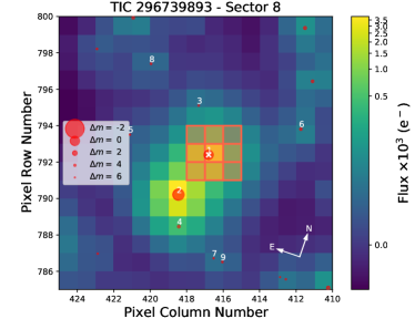
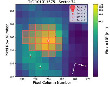
In this work, we specifically analyze the detrended Presearch Data Conditioning Simple Aperture Photometry (PDC-SAP) light curves for Sectors 8 and 34 (Smith et al., 2012; Stumpe et al., 2012, 2014) obtained from the Mikulski Archive for Space Telescopes (MAST)111https://mast.stsci.edu/portal/Mashup/Clients/Mast/Portal.html. After gathering this data, we normalize the detrended flux in so that the median for each sector is unity. In Figure 1, we show the TESS target pixel files (TPF) around the target star in Sectors 8 and 34, where orange outlines show the pixels used to create the TESS light curve. There are other point sources (notated by circular red points) that are located within the TESS apertures, so these needed to be subtracted from the SAP flux when creating the PDC-SAP flux.
2.1.2 Spitzer Light Curve
TOI 560 b was observed with Spitzer on 2019 August 20, using Director’s Discretionary Time (Crossfield et al., 2018). A single transit was observed using the 4.5 m channel (IRAC2, Fazio et al., 2004) in subarray mode with an integration time of 0.36 seconds. The transit observation spanned 6 hr 15 min totaling 823 frames with short observations taken before and after transit to check for bad pixels. Peak-Up mode was used to place the star as close as possible to the well-characterized “sweet spot” of the detector.
To extract photometry from the Spitzer observations, we use the Photometry for Orbits Eclipses and Transits (POET 222https://github.com/kevin218/POET) package (Cubillos et al., 2013; May & Stevenson, 2020). In summary, POET creates a bad pixel mask and discards bad pixels based on the Spitzer Basic Calibrated Data (BCD). Outlier pixels are also discarded using sigma-rejection. Then, the center of the point spread function (PSF) is determined using a 2-D Gaussian fitting technique. After the center of the PSF is found, the lightcurve is extracted using aperture photometry in combination with a BiLinearly-Interpolated Subpixel Sensitivity (BLISS) map described in Stevenson et al. (2012). The resulting data are then simultaneously fit with a model that accounts for both the lightcurve itself and a temporal ramp-like trend attributed to “charge trapping”. The posterior distribution is sampled using an MCMC algorithm with chains initialized at the best fit values.
Aperture photometry was performed with various aperture sizes (ranging from 2 - 6 pixels in increments of 1 pixel). Visual inspection of the raw data indicated the temporal ramp model was likely either linear or constant. The optimal aperture size was found to be 3 pixels as this size returned the lowest standard deviation of the normalized residuals (SDNR) for both ramp models. We then tested bin sizes of 0.1, 0.03, 0.01, and 0.003 pixels square for the BLISS map finding that a bin size of 0.01 minimized the SDNR. Both the linear ramp and constant models gave similar SDNR for these tests so we chose the constant model, the simplest of the two.
2.1.3 Las Cumbres Observatory Global network of Telescopes (LCOGT)
In 2019 and 2020, seven partial or full transit observations of TOI 560 b were collected with five observatory sites from the Las Cumbres Observatory Global network of Telescopes (LCOGT Brown et al., 2013). These observations are summarized in Table 2. Data were collected in either the B or Sloan filters with exposure times of 15 or 30 seconds to check for transit depth chromaticity such as would be produced by a false positive eclipsing binary scenario. For one transit (UT 2019/04/27), data were collected simultaneously in both filters. For a second transit (UT 2020/01/27), data was collected simultaenously in the same filter from two sites. The other five transits were observed in a single band at a single telescope/site. Data were analyzed using AIJ, and the data reduction was done using the BANZAI LCOGT facility pipeline (McCully et al., 2018).
2.1.4 The Perth Exoplanet Survey Telescope (PEST)
The Perth Exoplanet Survey Telescope (PEST) near Perth, Australia is a 0.3m telescope equipped with a 1530 × 1020 SBIG ST-8XME camera with an image scale of , resulting in a 31′′ × 21′′ field of view. Observations of a transit of TOI 560 b were obtained on UT 2020 January 14 in the Rc filter with an exposure time of 30 seconds. A custom pipeline based on C-Munipack was used to calibrate the images and extract differential photometry.
2.1.5 NGTS / Paranal
On UT 2019 December 07 the TOI 560 system was observed by the Next Generation Transit Survey (NGTS; Wheatley et al., 2018) using 4 telescopes (see Bryant et al., 2020), consist of 0.2 m diameter robotic telescopes, located at ESO’s Paranal Observatory, Chile. A custom NGTS filter in wavelength range 520-890 nm was used. A transit was detected and confirmed for planet b. The NGTS data were reduced using a custom aperture photometry pipeline version 2, which performs source extraction and photometry using the SEP Python library (Bertin & Arnouts, 1996; Barbary, 2016) and is detailed in (Bryant et al., 2020). The pipeline uses Gaia DR2 (Barbary, 2016; Gaia Collaboration et al., 2018) to automatically identify comparison stars which are similar in brightness, colour, and CCD position to TOI 560.
2.1.6 WASP Light Curves
2.2 Recon Spectroscopy
The purpose of reconnaissance spectroscopy is to provide spectroscopic parameters that will more precisely constrain the properties of planet host stars, to detect false positives caused by spectroscopic binaries as manifested by large (e.g. 1 km/s) RV changes and/or line-doubling in multi-epoch spectroscopy, and to identify stars unsuitable for precise RV measurements, such as rapid rotators.
2.2.1 NRES
Reconnaissance spectroscopy for TOI 560 was obtained with the Las Cumbres Observatory (LCOGT) Network of Robotic Echelle Spectrographs (NRES). NRES is a fiber-fed echelle spectrograph at several sites mounted on the respective LCOGT 1-m telescopes with wavelength range 380-860 nm and spectral resolution . Observations were executed at the Sutherland Observatory, South Africa, and the McDonald Observatory, USA, on the nights 2019 November 04, 2019 October 29, and 2019 May 12. We took dark, bias, flat, and arc lamp calibration images at the beginning of each night. The target was centered on one fiber, and the second fiber was used to observe a ThAr calibration lamp simultaneously. On each night, we took 3 consecutive exposures with 480 seconds on each individual spectrum. SNR for each night were 33, 30 and 33 respectively. We obtained the wavelength-calibrated spectra using the NRES commissioning IDL pipeline and obtained improved and stacked spectra for each night using the Stage2 IDL pipeline with a total integration time of 1440s and a resulting SNR of 35.
2.2.2 TRES
The Tillinghast Reflector Echelle Spectrograph (TRES; Fűrész, 2008) team obtained two reconnaissance (median SNR=33.25) spectra of TOI 560 near opposite quadratures of TOI 560 b (phases 0.25 and 0.72 on the initial Sector 8 released ephemeris) at 2019 April 16 04:37 and 2019 April 19 03:49 UT. TRES has a resolving power R 44,000 and the wavelength range of the spectrograph is 390-910 nm. The Stellar Parameter Classification (SPC) tool specifically uses a 310 Angstrom region of the spectrum (5050-5360 Angstroms) to derive stellar parameters (3.1.1). Spectra are processed following methods described in Buchhave (2010).
2.3 High Resolution Imaging
High-resolution imaging is used to obtain images of faint companions located near bright target stars. Typical targets are stars with companions including exoplanets and circumstellar structures and disks of gas and dust. In seeing-limited imaging, a faint companion could be swamped and lost in the noise of scattered light in the point spread function (PSF) wings of the target star. High contrast imaging methods – speckle imaging and adaptive optics – were designed to mitigate the impact of target star scattered light at the position of the companion, in order to make the companion detectable against the residual PSF noise (e.g. Guyon, 2005; Mawet et al., 2014; Lafrenière et al., 2007; Marois et al., 2006).
High-contrast imaging of TESS candidates is crucial to ensure that the target is not a false positive from a background eclipsing binary, and to ensure that the planetary radius is unbiased by additional, unidentified, flux sources within the aperture. Spatially close stellar companions can create a false- positive transit signal if, for example, the fainter star is an eclipsing binary (EB). However, even more troublesome is “third-light” flux contamination from a close companion (bound or line of sight) which can lead to underestimated derived planetary radii if not accounted for in the transit model (e.g., Ciardi et al., 2015) and even cause total non-detection of small planets residing within the same exoplanetary system (Lester et al., 2021). Given that close bound companion stars exist in nearly one-half of FGK type stars (Matson et al., 2018) high-resolution imaging provides crucial information toward our understanding of exoplanetary formation, dynamics and evolution (Howell et al., 2021). Herein we present high-contrast imaging of TOI 560 obtained with Gemini with NIRI and Zorro and the SOAR telescope respectively.
2.3.1 Gemini North / NIRI
We searched for close visual companions to the target using high resolution imaging with both AO and speckle imaging at Gemini. The AO and speckle images are highly complementary: the speckle images reach higher resolutions in the optical, while the AO images reach deeper sensitivities beyond a few hundred mas in the near-IR, and are therefore more sensitive to more widely separated low-mass stars. We collected high-resolution AO images of TOI 560 with Gemini/NIRI (Hodapp et al., 2003) on 2019 May 26. Given that the star is bright in the K band, we collected images with individual exposure time 0.9s with the Br filter (2.166m), to avoid saturating the detector. Our sequence consisted of nine such images, with the telescope dithered in a grid pattern between each frame, and we also collected daytime flats. The science images themselves can be used to construct a sky background frame, by median combining the dithered images.
2.3.2 Gemini South / Zorro
TOI 560 was observed twice on 2020 March 16 and 2019 May 22 UT using the Zorro speckle instrument on the Gemini South 8-m telescope333https://www.gemini.edu/sciops/instruments/alopeke-zorro/. Six sets of 1000 by 0.06 sec exposures were collected for TOI 560 and processed with Fourier analysis in our standard reduction pipeline (see Howell et al., 2011).
2.3.3 SOAR telescope
We searched for stellar companions to TOI 560 with speckle imaging on the 4.1-m Southern Astrophysical Research (SOAR) telescope (Tokovinin, 2018) on 18 May 2019 UT, observing in Cousins I-band, a similar visible bandpass as TESS. This observation was sensitive to a 7.5-magnitude fainter star at an angular separation of 1′′ from the target. More details of the observation, data reduction and analysis are available in Ziegler et al. (2020).
2.4 Radial Velocities
Herein we present ground-based precise radial velocity observations collected with high-resolution echelle spectrographs PFS, HIRES, and MINERVA-Australis at visible wavelengths, and iSHELL in the NIR in the following subsections.
2.4.1 iSHELL RVs
We have gathered a total of 204 observations of TOI 560 over 30 nights using the iSHELL instrument at NASA InfraRed Telescope Facility (IRTF) atop Maunkea, Hawaii, USA from UT 26 January 2020 to UT 29 May 2021. We observe with iSHELL in KGAS mode covering the wavelengths of 2.18–2.47 m. Our exposure times were always set at 300 seconds, and were repeated anywhere from 6–14 times consecutively per night to attempt obtaining a signal-to-noise ratio (SNR) per spectral pixel of 120, though our actual results varied from 46-152 due to variable seeing and atmospheric transparency conditions. A methane isotopologue () gas cell is used in the instrument (Plavchan et al., 2013; Cale et al., 2019) to constrain the line-spread function (LSF) and provide a common reference for the optical path wavelength. Along with each set of exposures within a night, we also collect a set of 5x15-second flat-field images with the gas cell removed for data reduction purposes, and particularly to mitigate flexure-dependent and time-variable fringing present in the spectra. In Cale et al. (2019), the RV pipeline is adapted from the CSHELL RV code described in Gao et al. (2016), and the CSHELL code was re-written in a Python script pychell444 Documentation: https://pychell.readthedocs.io/en/latest/ to adapt to iSHELL’s larger spectral grasp with multiple orders.
When the light passes through a gas cell and an echelle spectrograph, the spectrum consists of multi-order spectra of the target with the gas spectrum super-imposed, which can be used to subtract off instrument systematic shifts in the wavelength solution and changes in the line spread function (Butler et al., 1996). We extract our spectra following the general procedures outlined in Cale et al. (2019). For each of the 29 orders in the regime that we observe between 2.18–2.47 m, we do optimal spectral extraction (weighted summation) so that in each column eventually we get a single value, which gives us a one-dimensional spectrum for each order.
The extracted spectra from pychell were forward-modeled and analyzed using the methods outlined in Cale et al. (2019), and the updated methods described in Reefe et al. (submitted, 2021), briefly described herein. We forward model the extracted spectra independently for each order to account for the stellar spectrum, gas cell, telluric absorption, the line spread function, and the spectral continuum to construct a complete spectral model. We find that pychell performs better when providing a synthetic stellar template for the stellar model to start from, which is based on properties of the host-star.
We assume a solar metallicity and gravity, and we explore synthetic models 500 K from an initial temperature of 4700 K, based upon the EXO-FOP-TESS values, in increments of 100 K to identify the optimal synthetic stellar template that produces the lowest rms flux residuals in forward modeling our extracted spectra. We use the Spanish Virtual Observatory’s (SVO) BT-Settl models accessible from their web server555http://svo2.cab.inta-csic.es/theory/newov2/index.php?models=bt-settl, which we further refine by Doppler broadening the spectrum to the rotational velocity of the star (3.1 km s-1), as found by TRES extracted spectra (3.1.1). We find that the synthetic model minimizes the flux residuals of our observed iSHELL spectra, even though hotter than our adopted stellar temperature, and we use this stellar template as our initial stellar spectrum model guess. Barycenter velocities are also generated as an input via the barycorrpy library (Kanodia & Wright, 2018).After each order is forward-modeled, we generate one RV measurement per-order and per-exposure. We optimally co-add RVs across orders and exposures within a night using the same procedures as in Cale et al. (2019).
We have filtered out three individual spectra from UT 7 March 2020 and three more individual spectra from UT 8 March 2020, due to modeled RVs that were in disagreement with other spectra from the same night by 1 km s-1. We suspect this is due to an initially poor seeing on the nights of observation of that was later improved to , giving us an overall SNR of only 54 and 46 respectively for the nights. Finally, we discard nights with RV uncertainties 20 m/s.
2.4.2 PFS RVs
We obtained 14 RVs of TOI 560 from the Planet Finder Spectrograph (PFS) on the 6.5m Magellan II telescope at Las Campanas Observatory in Chile. These spectra were reduced and RVs were extracted and published in the Magellan-TESS Survey I paper (Teske et al., 2021). PFS Spectrograph has resolution of R=120,000 and wavelength range of nm.The observations were carried out between UT 2019 April 18 and May 24.
2.4.3 HIRES RVs
We include 14 Keck-HIRES (Vogt et al., 1994) observations of TOI 560 in our analyses. Keck-HIRES is located atop Maunkea, Hawaii, USA with spectral resolution R= 67,000. The majority of these observations took place between UT 2019 October 20 and 2020 January 21, with the final night contemporaneous with the start of iSHELL RVs. Exposure times range from 204–500 seconds, yielding a median SNR 234 at 550 nm per spectral pixel. HIRES spectra are processed and RVs computed via methods described in Howard et al. (2010).
2.4.4 Minerva-Australis RVs
Minerva-Australis collected two nights of observations of TOI 560 (Addison et al., 2019, 2021b). Minerva-Australis consists of an array of four independently operated 0.7 m CDK700 telescopes situated at the Mount Kent Observatory in Queensland, Australia (Addison et al., 2019). Each telescope simultaneously feeds stellar light via fiber optic cables to a single KiwiSpec R4-100 high-resolution () spectrograph (Barnes et al., 2012) with wavelength coverage from 480 to 620 nm. We obtained a total of 10 individual spectra of TOI 560 on UT 2019 May 23 and UT 2019 May 29 using three and two of the four Minerva-Australis telescopes respectively – twice per night per telescope – and exposure times of 30-60 minutes. Wavelength calibration is achieved using a simultaneous Th-Ar calibration fibre. Radial velocities were derived by cross-correlation, where the template being matched is the mean spectrum. Given that only two nightly RV data points were obtained, we do not include the Minerva-Australis RVs in the remainder of the analysis presented herein.
3 Analysis
In this Section, we present our analysis of the TOI 560 system. In Section 3.1 we present the stellar host characterization. In Section 3.2 we present the light curve analysis, including the discovery of the transits of TOI 506 c, false-positive vetting metrics, and characterization of the out-of-transit stellar activity in both the TESS and SuperWASP light curves. Finally, in Section 3.3 we present the analysis of the TOI 560 RV data aided with a stellar activity model constrained by the light curve analysis.
3.1 Stellar Host Characterization
Our analysis and understanding of exoplanets is directly dependent on our understanding of their host stars (e.g. Ballard et al., 2014). We measure planetary masses and radii in terms of their host stars’ masses and radii, we derive elemental abundance ratios from those in the atmosphere of their host star, and we infer surface temperatures and conditions informed by their host stars’ luminosities, ages, and levels of activity. Host star properties are precisely determined through spectroscopic analysis; therefore, herein we analyze in turn the reconnaissance spectra of TOI 560, fitting bulk stellar properties from the broadband spectral energy distribution (SED), and solidify our analysis with high contrast imaging to exclude faint flux-contaminating companions.
3.1.1 Reconnaissance Spectroscopy
The reconnaissance spectroscopy observations reveal a typical late K dwarf. Stellar parameters from the NRES spectra were obtained using SpecMatch (Vanderburg et al., 2019b), and summarized in Table 11. For the TRES spectra, there is a small velocity difference that is consistent with the photometric ephemeris, given that the data were collected approximately at opposite quadratures. In Table 12, the results for the stellar parameters for the two TRES observations are presented, as well as values from the Stellar Parameter Classification (SPC) tool (Buchhave et al., 2012, 2014). Given the absence of any large bulk RV changes or spectroscopic binarity, we do not co-add the multi-epoch spectroscopy to improve the cumulative SNR (and consequently reduce the stellar parameter uncertainties), due to current systematic limitations in these approaches (e.g., Duck et al., 2022). We adopt floor errors of in , 0.10 in , 0.08 in , and 0.5 km/s in . Note that does not include a correction for the contribution of macroturbulence, and the velocities in Table 12 are on the TRES native system and do not correct for the gravitational redshift. The TRES and NRES analyses yield consistent stellar characterization, with the SPC analysis favoring a slightly higher but not statistically significant rotational velocity and metallicity.
3.1.2 Bulk Stellar Properties
We undertake two independent analyses of the broadband spectral energy distribution (SED) of the star, and we describe each in turn. The first approach is particularly useful for assessing the evidence for any near-UV excess from consideration of the broadband photometry alone. Our second approach is used for our adopted final stellar parameters and is based upon holistic modeling of the SED jointly with the transit light curves and model isochrones.
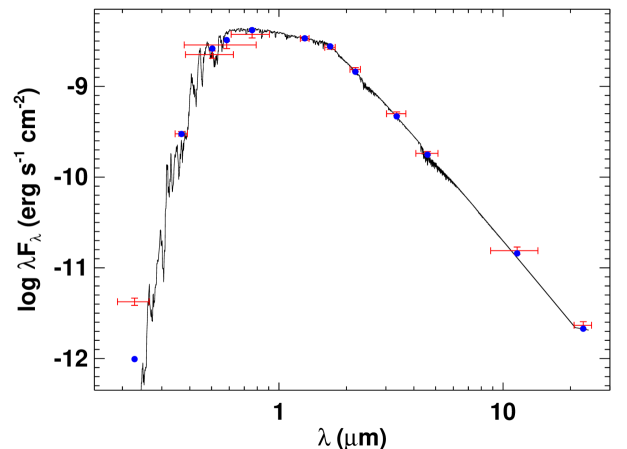
First, we performed a single-parameter fit of the SED of the star together with the Gaia EDR3 parallax (with no systematic offset applied; see, e.g., Stassun & Torres, 2021a), in order to determine an empirical measurement of the stellar radius and following the procedures described in Stassun & Torres (2016); Stassun et al. (2017, 2018). We use the magnitudes from the compilation of Mermilliod (2006), the magnitudes from 2MASS, the W1–W4 magnitudes from WISE (Wright et al., 2010), the magnitudes from Gaia, and the NUV magnitude from GALEX. Together, the available photometry spans the full stellar SED over the wavelength range 0.2–22 m (see Figure 2). We used a NextGen stellar atmosphere model, fixing the model effective temperature (), metallicity ([Fe/H]), and surface gravity () to the values derived from the TRES SPC analysis in 3.1.1 and Table 12. The remaining free parameter is the extinction , which we fixed at zero given the proximity of the TOI 560 system to Earth. The resulting fit (Figure 2) has a reduced of 1.7, excluding the GALEX NUV flux which indicates a moderate level of activity (see below). Integrating the (unreddened) model SED gives the bolometric flux at Earth, erg s-1 cm-2. Taking the and together with the Gaia parallax, gives the stellar radius, R⊙ (consistent with the NRES analysis). In addition, we can estimate the stellar mass from the empirical relations of Torres et al. (2010), giving M⊙, which is consistent with the less precise but empirical estimate of M⊙ obtained directly from together with the spectroscopic .
Second, we determine characteristics of the host star, such as effective temperature, gravity, metallicity, etc., by performing a joint amoeba fit followed by Markov-Chain Monte Carlo (MCMC) posterior sampling of both stellar properties and planet properties of TOI 560 b&c assuming a two-planet, single-star scenario (from the TESS transit data) simultaneously with EXOFASTv2. EXOFASTv2 is an (IDL) framework for MCMC simulations of exoplanet transits and radial velocities created by Eastman et al. (2013). Details on the planet transit analysis are in the next section 3.2, but here we present the stellar modeling analysis steps. We start the MCMC with as few assumptions as possible – namely, we place no priors on the spectral type. To ensure we cover an adequate portion of parameter space to find a believable result, we employ parallel tempering with eight parallel threads, following Eastman et al. (2019). We place priors on V-band extinction, parallax, and metallicity summarized in Table 5 along with the priors used in the transit analysis. We simultaneously fit with Mesa Isochrones and Stellar Tracks (MIST) and a spectral energy distribution (SED) function. We then use the posteriors of this run as priors for a second iteration MCMC analysis to examine the stability of the solution and adopt our final stellar parameters.
The results of our EXOFASTv2 stellar characterization are shown in and Table 3. The analysis yields a typical K dwarf consistent with the reconnaisance spectroscopy and SED analysis presented in 3.1. We provide two separate estimates for and corresponding to the MIST results and the SED results, respectively. SED results are marked with the subscript SED while MIST results have no subscript. We adopt the MIST values for the remainder of the analysis, but both sets of values are consistent with one another and with the analysis carried out with the SED and reconnaissance spectroscopy. Finally, we note that the age estimate from EXOFASTv2 shown in Table 3 is drawn from a very flat posterior distribution and is not a reliable estimate; e.g. the stellar age is unconstrained from this particular analysis. Instead, we adopt the final rotation period of 12.20.1 days as described in 3.1.3.
| Stellar Parameters | Units | Values | ||
|---|---|---|---|---|
| M∗ | Mass (M⊙) | |||
| R∗ | Radius (R⊙) | |||
| R∗,SED | Radius666This value ignores the systematic error and is for reference only (R⊙) | |||
| L∗ | Luminosity (L⊙) | |||
| FBol | Bolometric Flux ((erg/s)/cm2) | |||
| Density (g/cm3) | ||||
| g | Surface gravity (cm/s2) | |||
| Teff | Effective Temperature (K) | |||
| Teff,SED | Effective Temperature777This value ignores the systematic error and is for reference only (K) | |||
| Metalicity (dex) | ||||
| Initial Metallicity888The metallicity of the star at birth | ||||
| Age | Age999This posterior is relatively flat and unconstrained, and does not take into account the stellar rotation period analysis estimated in 3.1.3 and /or Figure 3 (Gyr) | |||
| EEP | Equal Evolutionary Phase101010Corresponds to static points in a star’s evolutionary history. See 2 in Dotter (2016). | |||
| Av | V-band extinction (mag) | |||
| SED photometry error scaling | ||||
| Parallax (mas) | ||||
| d | Distance (pc) | |||
| Wavelength Parameters | Units | B | R | z’ |
| linear limb-darkening coeff | ||||
| quadratic limb-darkening coeff | ||||
| Dilution from neighboring stars | – | – | – | |
| Telescope Parameters | Units | HIRES | PFS | iSHELL |
| Relative RV Offset (m/s) | ||||
| RV Jitter (m/s) | ||||
| RV Jitter Variance |
Finally, TOI 560 has a GAIA RUWE value of 1.030, which is consistent with a single star (Stassun & Torres, 2021b). The RUWE statistic is an indication of the goodness of fit of the astrometric solution, and values 1.4 have been shown to be associated with unresolved binaries. A search of EDR3 also shows no stars with similar parallaxes within 75’, so TOI 560 likely does not possess any distant, resolved binary companions either.
3.1.3 Age Metrics – Is TOI 560 a young system?
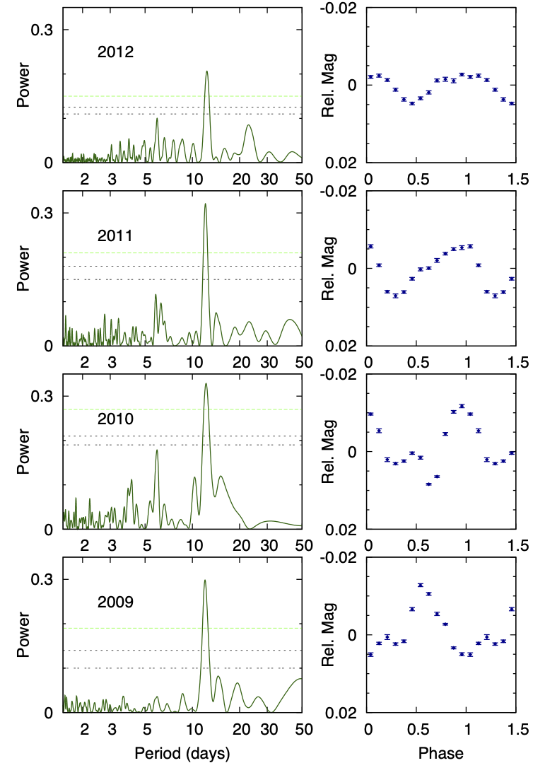
Lomb-Scargle periodograms of the SuperWASP seasonal light curves show a clear and consistent rotation period in each season for TOI 560 of 12 days, with evolution of the light curve features between seasons (Figure 3. The periodogram peak is statistically significant in all seasons (p-value1%) and the average periodogram peak period from all four seasons yields a rotation period of 12.20.1 days. We next use the star’s NUV excess (Fig. 2) to estimate the star’s rotation and age via empirical rotation-activity-age relations. The observed NUV excess implies a chromospheric activity of via the empirical relations of Findeisen et al. (2011), which is fully consistent with the measured value of from Gomes da Silva et al. (2021) and -4.60 from our HIRES spectra. The HIRES and TRES spectra show core Ca II HK flux in emission, consistent with this moderate level of activity. This value of in turn implies a stellar rotation period of d via the empirical relations of Mamajek & Hillenbrand (2008). This rotation period estimate is also consistent with that estimated from the spectroscopic and , which gives d. Thus the observed photometric modulation, NUV excess, and the observed rotational velocity all yield consistent rotation periods. This establishes the rotation period of the TOI 560 host star.
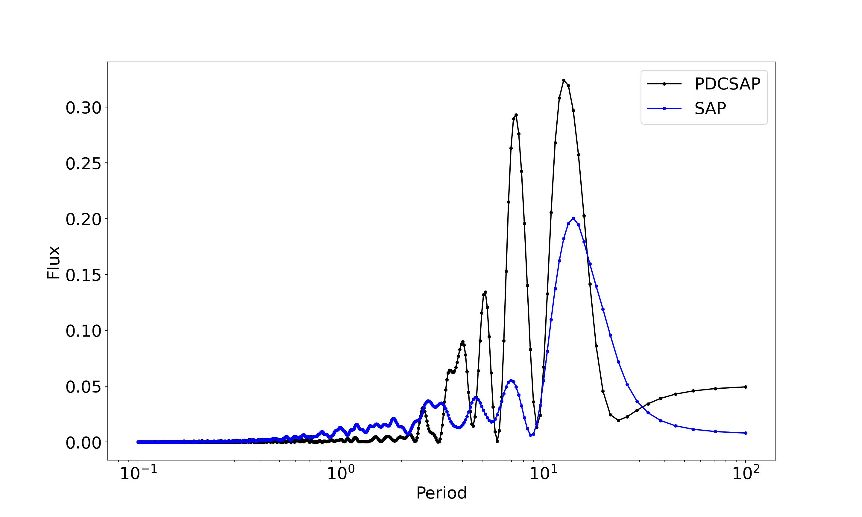
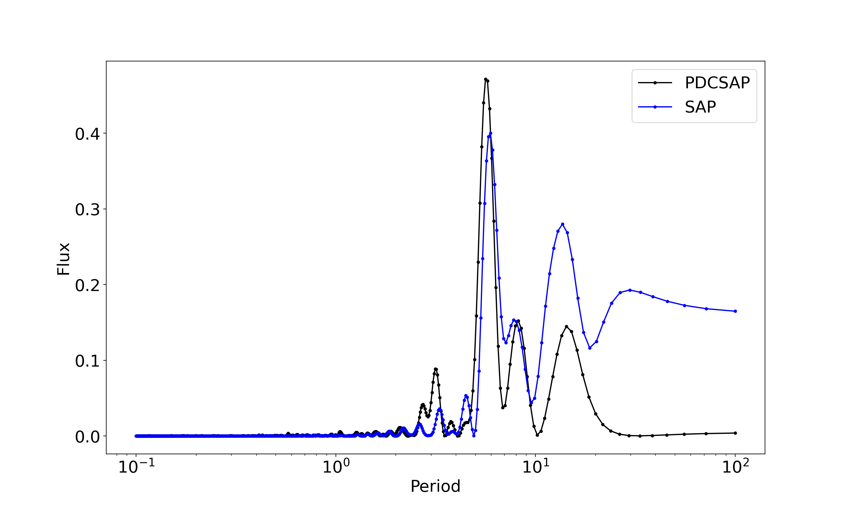
However, this 12-day rotation period is roughly a factor of 2 slower than that reported by Canto Martins et al. (2020), who report a “dubious” rotation period 7.17d from their independent TESS light curve analysis. We can also estimate rotation periods for TOI 560 by performing Lomb-Scargle (LS) periodograms (Lomb, 1976; Scargle, 1982) of the TESS Sector 8 and 34 light curves of TOI 560. In Figure 4, the TESS light curves contain significant peaks at 12.7 days for PDCSAP and 14.1 days for SAP, both for the Sector 8 respectively, that are not obvious integer fraction multiples of one another nor of 7.17d; we do find a secondary peak at 7.29 days for the Sector 8 light curve, consistent with Canto Martins et al. (2020). However, the dominant period in the Sector 8 light curve at 12.7 days is reasonably consistent with the WASP, NUV, and rotational velocity inferred rotation periods. A more detailed FF’ modeling of the TESS light curves in 3.2.3 with a Gaussian process and uniform rotation period prior from 2–20 days also favors a rotation period of 7.13 days, also consistent with Canto Martins et al. (2020). However, given that the time segments of the TESS light curve in-between data downlinks are themselves 12 days in time baseline, we find that the TESS light curves themselves are insensitive to a 12-day rotation period and are thus not reliable; the 7.1 and 5.6 day power in the TESS light curves may be from a combination of the first harmonic of the stellar rotation period at , potentially the spot evolution timescale, and the pre-search data conditioning of the TESS PDC-SAP light curves. Thus, we adopt the rotation period of 12.2 days from the SuperWASP light curves in the remainder of our analysis.
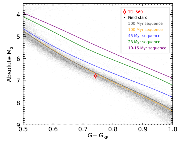
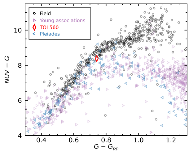
For this rotation period, using the age-rotation relation from Mamajek & Hillenbrand (2008) based upon the power-law model of Barnes (2007), we derive a stellar age estimate of Myr. However, Curtis et al. (2020) have recently shown that for K dwarfs like TOI 560, there is an age-rotation “pile-up” at rotation periods of 10–15 days where the spin-down of K dwarfs stalls between ages 0.6–1.4 Gyr, before resuming for ages 1.4 Gyr. We also verified whether TOI 560 may be a plausible member of a nearby moving group or association with the BANYAN (Gagné et al., 2018a) tool which compares the Galactic coordinates and space velocities of known stellar associations and assigns a membership probability based on Bayes’ theorem with the option to marginalize over unknown quantities such as heliocentric radial velocities. We find a negligible membership probability to all 27 young associations included in BANYAN . We also compared the and of TOI 560 to those of 1 000 moving groups and open clusters identified in the literature so far within 500 pc of the Sun, and we find no plausible association to which TOI 560 may belong to. Inspecting the position of TOI 560 in a Gaia eDR3 (Gaia Collaboration et al., 2018) color-magnitude diagram (Figure 5) reveals a picture consistent with an age of at least 100 Myr. TOI 560 has been detected in GALEX DR5(Bianchi et al., 2011), and its position in a GALEX-Gaia color-color diagram (Figure 6) shows that it located on the UV-bright end of field stars and on the UV-faint end of the Pleiades members with similar Gaia eDR3 color (which tracks spectral types), thus indicating that TOI 560 is likely older than the Pleiades, but plausibly on the younger end of the age distribution of field stars, and consistent with the rotation-based age estimate. Additionally, there is no lithium detected, consistent with this star not being 100 Myr (Delgado Mena et al., 2015). We thus conclude from the rotation period of TOI 560 and the K dwarf rotational evolution pile-up that TOI 560 possesses and age between 150 Myr and 1.4 Gyr.
3.1.4 High Contrast Imaging
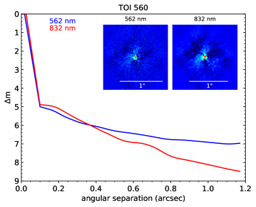
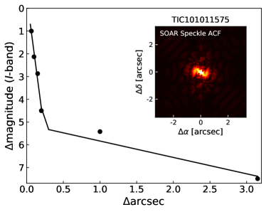
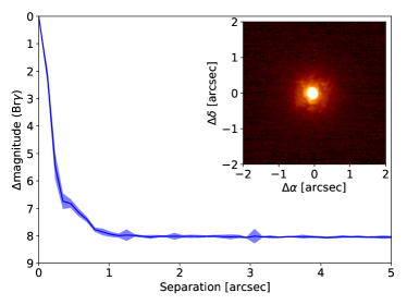
For the Gemini/NIRI observations, we carried out the data reduction using a custom set of IDL codes, with which we removed bad pixels, sky-subtracted and flat-corrected the frames, and then aligned the stellar position between frames and co-added the images (Hodapp et al., 2003). For Gemini South, we utilize only the observations from May 2019, as the March observations had poorer seeing and sky conditions, albeit giving similar results to those obtained about a year earlier. Zorro provides simultaneous speckle imaging in two bands (562 nm and 832 nm) with output data products including a reconstructed image in Figure 7 with robust contrast limits on companion detection (e.g. Howell et al., 2016).
For our Gemini/NIRI observation, we did not identify visual companions anywhere in the field of view, which extends to at least in all directions from the target star, and TOI 560 appears single to the limit of the Gemini/NIRI resolution. The sensitivity as a function of separation is shown in Figure 7, along with an image of the target. The images are sensitive to companions 8mag fainter than the host star in the background limited regime (beyond ). For our Gemini South observations, Figure 7 shows our final 5- contrast curves and the reconstructed speckle images. We find that TOI 560 is single to within the contrast limits achieved by the observations. No companion is identified brighter than 5-8 magnitudes below that of the target star from the diffraction limit (20 mas) out to . At the distance of TOI 560 (d=31 pc) these angular limits correspond to spatial limits of 0.6 to 37 AU. Finally, for our SOAR observation, Figure 7 shows the 5 detection sensitivity and speckle auto-correlation functions from the observations. No nearby stars were detected within 3″of TOI 560 in the SOAR observations.
3.2 Light curve analysis
In this section, we vet against false positive scenarios using different tests in 3.2.1, and then we analyze the TESS sector 34 light curve to discover TOI 560 c in 3.2.2. After that, we apply our GP analysis to the light curves in 3.2.3, and using EXOASTv2 in 3.2.4, we jointly analyze the sector 8 and 34 TESS light curves as a 2-planet system.
3.2.1 Vetting against False Positive
Before investing detailed resources in the RV analysis of a TESS candidate planetary system, it is useful to rule out false-positive scenarios caused by eclipsing binaries and other systematics, and there are numerous diagnostics that we employ using the TESS light curves alone. We ran two separate vetting analyses on the TOI 560 data gathered by TESS.
The first of our vetting tests was performed with the EDI-Vetter Unplugged tool (Zink et al., 2020)111111https://github.com/jonzink/EDI_Vetter_unplugged. EDI-Vetter Unplugged checks for several diagnostics that could be indicative that the target is a false positive. First, EDI-Vetter checks for neighboring flux contamination from nearby stars in the sky, to make sure that the signal is indeed correlated with the expected target; this is necessary due to the large angular size of TESS pixels. Second, it examines the abundance of outliers from the transit model, as well as the validity of each individual transit – e.g. odd/even test, if transits fall into masked data gaps. Third, it also searches for the statistically significant presence of any secondary eclipses, which could indicate an eclipsing binary. Other measures that are considered are the similarities between transit signals, the phase coverage of transit signals, and the relative length of transit duration in comparison to period. The results of our EDI-Vetter analysis are in table 4 in section 4.
Second, we also scrutinized the TESS light curves using the Discovery and Vetting of Exoplanets (DAVE) software (Kostov et al., 2019) developed at the NASA Goddard Space Flight Center. This tool evaluates similar criteria as the EDI-Vetter tool, such as odd/even transit differences and secondary eclipses, but also searches for any photocenter shift, or the difference between the TIC position and the measured photocenter of the transits during transit, which is often also a diagnostic of a blended eclipsing binary.
In our EDI-Vetter analysis, two of the criteria were flagged as a potential false-positive: the uniqueness of the transit signal and the planet masks (Table 4). However, the latter is due to the system being a multiplanet system, with two different transiting planets, and the former a transit of TOI 560 c falling into the data download gap of Sector 8. In our DAVE analysis, we show full transit data and phased odd/even, secondary, tertiary, and positive transits for each sector in figures 38 and 39. We see little to no variation between the primary odd and even transits, and we see no statistically significant drop in flux during the expected ephemerides for a secondary eclipse or tertiary transit. However, we note the appearance of an odd-even transit depth difference for TOI 560 b. Due to the youth of the star, there is significant out of transit variability from the star that is not filtered out by the DAVE vetting tool. This in turn impacts its transit depth determination, resulting in the even-odd discrepancy. Thus, we effectively ignore this metric present in the DAVE tool as a potential sign of a false-positive, which is supported by the multi-planet nature of the system.
We also see no statistically significant positive flux variation that could be indicative of lensing between eclipsing binary stars. The evaluation of the photo-center shift during transit helps validate that the transit belongs to the target star, and not a faint companion. Photo-center difference plots for each sector are shown in Figure 40, and overall show no major variations between the expected and observed locations. Thus, this vetting analysis from DAVE and EDI-Vetter, combined with our high-contrast imaging, rules out a blended or background eclipsing binary companion, and confirms that the transit signals originate from TOI 560, and not another nearby point source. Further, when combined the increasingly low probability (e.g. , Lissauer et al., 2012) that multiple blended or background eclipsing binaries would be spatially coincident with TOI 560 and produce two different eclipsing signals near a 3:1 orbital period coincidence, we can conclude that TOI 560 is the host of the two eclipsing companions. We next turn to presenting our results on constraining the masses of TOI 560 b and c.
| Vetting Report | Sector 8 | Sector 34 |
|---|---|---|
| Transit Count | 6 | 6 |
| Flux Contamination | False | False |
| Too Many Outliers | False | False |
| Too Many Transits Masked | False | True |
| Odd/Even Transit Variation | False | False |
| Signal is not Unique | True | True |
| Secondary Eclipse Found | False | False |
| Low Transit Phase Coverage | False | False |
| Transit Duration Too Long | False | False |
| Signal is a False Positive | True | True |
3.2.2 The discovery of TOI 560 c
With the release of the TESS Sector 34 light curve, we readily identified by eye two transits of a second planet candidate with an orbital period of 18.9 days. Several other teams independently identified this second transiting planet during our analysis, and was identified by the TESS mission as TOI 560 c ( days). After masking the transits of TOI 560 b ( days), we computed BLS (Kovács et al., 2002) and TLS (Hippke & Heller, 2019) periodograms and phased LCs of the Sector 34 light curve in Figure 8. Due to unfortunate timing, TOI 560 c did not transit in the Sector 8 TESS light curve (Figure 8). We also excluded a period for TOI 560 c of one-half its value, as a third transit of TOI 560 c could have occurred during a data down-link data gap in the TESS Sector 34 light curve. However, under that scenario, a transit of TOI 560 c would have occurred in the Sector 8 light curve, which is ruled out.
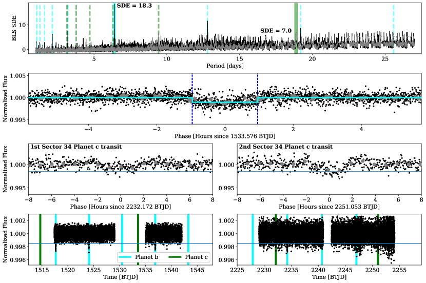
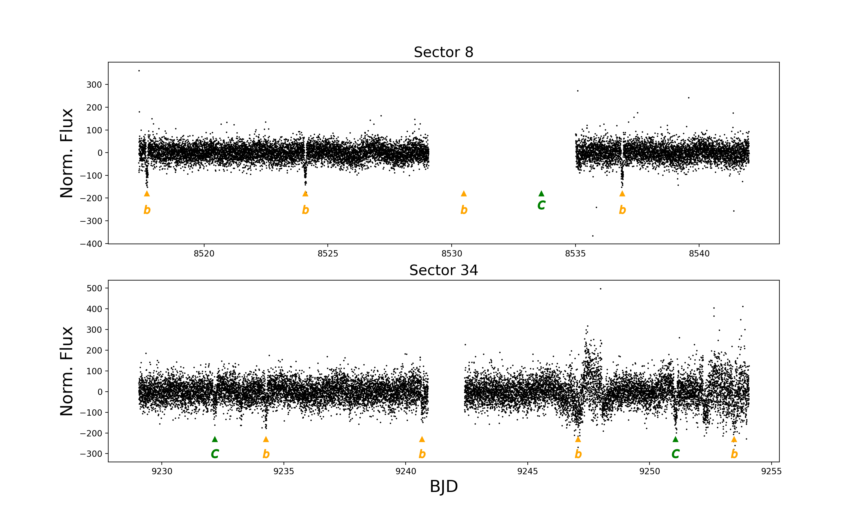
Note: the time units of BTJD are BJD-2457000.0 days. Second Row: Phased light curve for the two transits of TOI 560 c in the Sector 34 TESS light curve as unbinned black and binned (one hour) grey dots, plotted as a function of time in hours on the horizontal axis with respect to the transit conjunction time, and the normalized flux on the vertical axis. A teal transit model is overlaid. The blue dashed vertical lines correspond to the time of conjunction and transit ingress and egress. Third Row: Same as the second row, but the individual transits of TOI 560 c are plotted separately. Fourth Row: The Sector 8 (left) and 34 (right) light curve of TOI 560 with the transit times of TOI 560 b and c marked in teal and green respectively, plotted as a function of time and normalized flux. This shows that TESS just missed observing TOI 560 c during this initial sector. The horizontal blue line is a line corresponding to 2 ppt, the approximate depth for TOI 560 c.
The model parameters and prior distributions used in our RV model that considers the transiting b and c planets, as
3.2.3 GP Analysis of the Light Curves
Stars are not uniform disks; they exhibit RV variations from rotationally-modulated activity, e.g. star spots and plages on the surface of the star (Dumusque et al., 2011b, a; Fischer et al., 2016; Plavchan et al., 2015b, and references therein). Depending on the temperature contrast between magnetically active regions and the surrounding photosphere of the star, these active regions will induce an apparent RV shift that is quasi-periodic as the active regions evolve on time-scales distinct from the rotation period of the star. Gaussian processes (GPs) have been widely and successfully employed in modeling the apparent RVs due to stellar activity (Haywood, 2015).
The same active regions also give rise to photometric variations from the hemisphere visible to the observer. Thus, we can model the light curves of TOI 560 out of transit with a GP, and use the light curve hyperparameter posteriors to constrain the GP model hyper-parameter priors for our subsequent analysis of the RVs, following the technique (Aigrain et al., 2012). This method allows us to generate what a simulated RV curve would look like from the stellar activity:
| (1) |
Here, F is the photometric flux, is the derivative of F with respect to time, f represents the relative flux drop for a spot at the center of the stellar disk, and is the stellar radius.
Our Gaussian process kernel describes the functional covariance between any two measurements separated in time. The kernel by definition must be a square, symmetric covariance matrix “K” of length equal to the number of observations. We follow Haywood (2015) who introduced the quasi-periodic (QP) Kernel composed of a decay and periodic term:
| (2) |
where: , Here, typically represents the stellar-rotation period, the mean spot lifetime, and is the relative contribution of the periodic term, which may be interpreted as a smoothing parameter (larger is smoother). is the amplitude of the auto-correlation of the activity signal. The set of constitute the set of GP model hyper-parameters that are constrained by the data. There exist families of stellar activity models that generate a particular covariance matrix given by a specific set of hyper-parameters, and thus GPs are a flexible framework for characterizing the non-deterministic time evolution of stellar activity. The analysis does enable us to estimate the expected amplitude of the RV variations at wavelengths comparable to the light curve observations, , but we end up not using that amplitude in our RV modeling. Instead, we do use the analysis to get estimates of the remaining hyperparameters, particularly , , for use in the RV analysis.
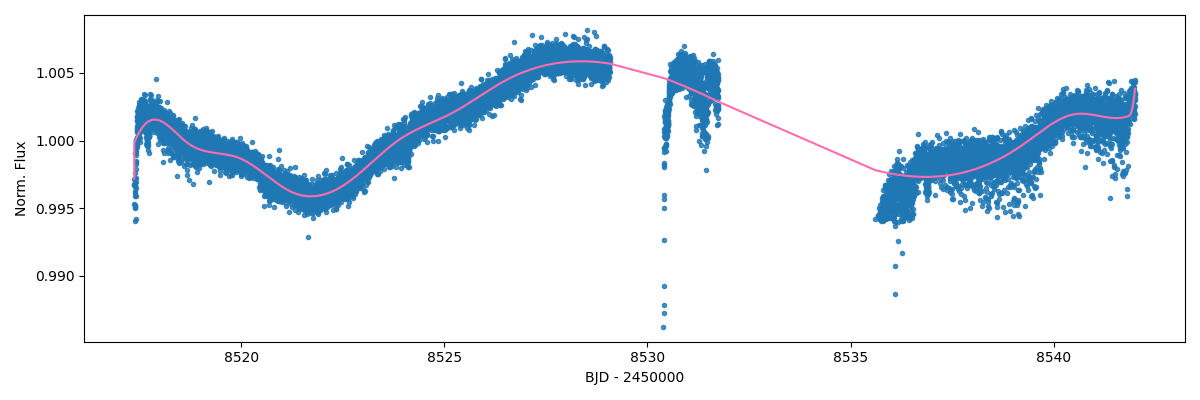
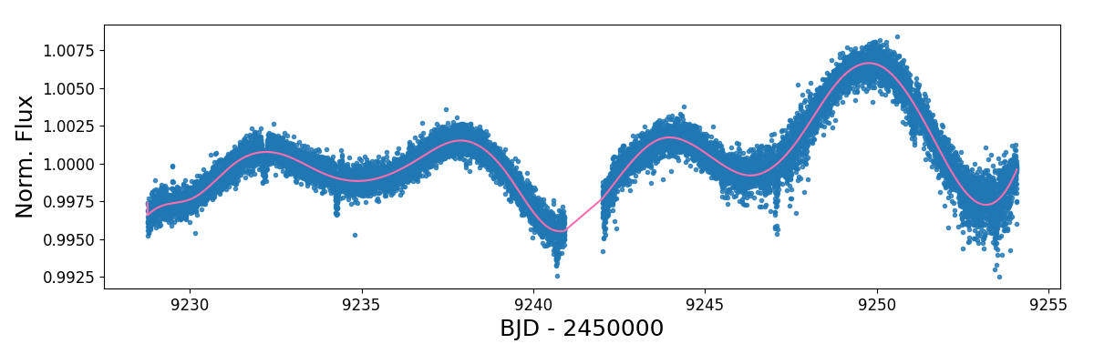
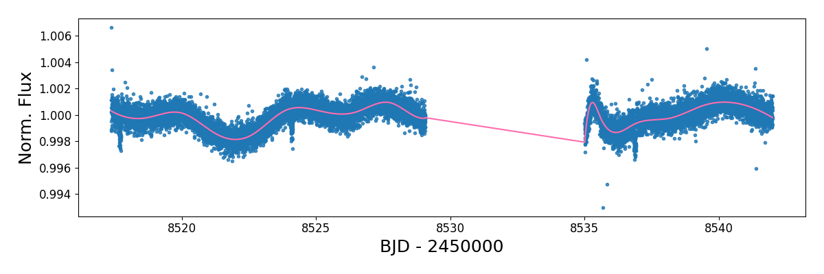
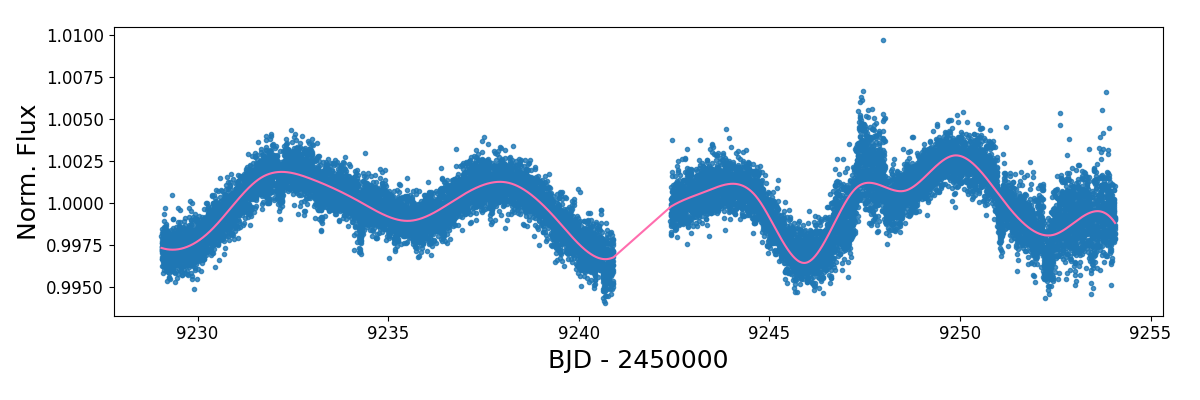
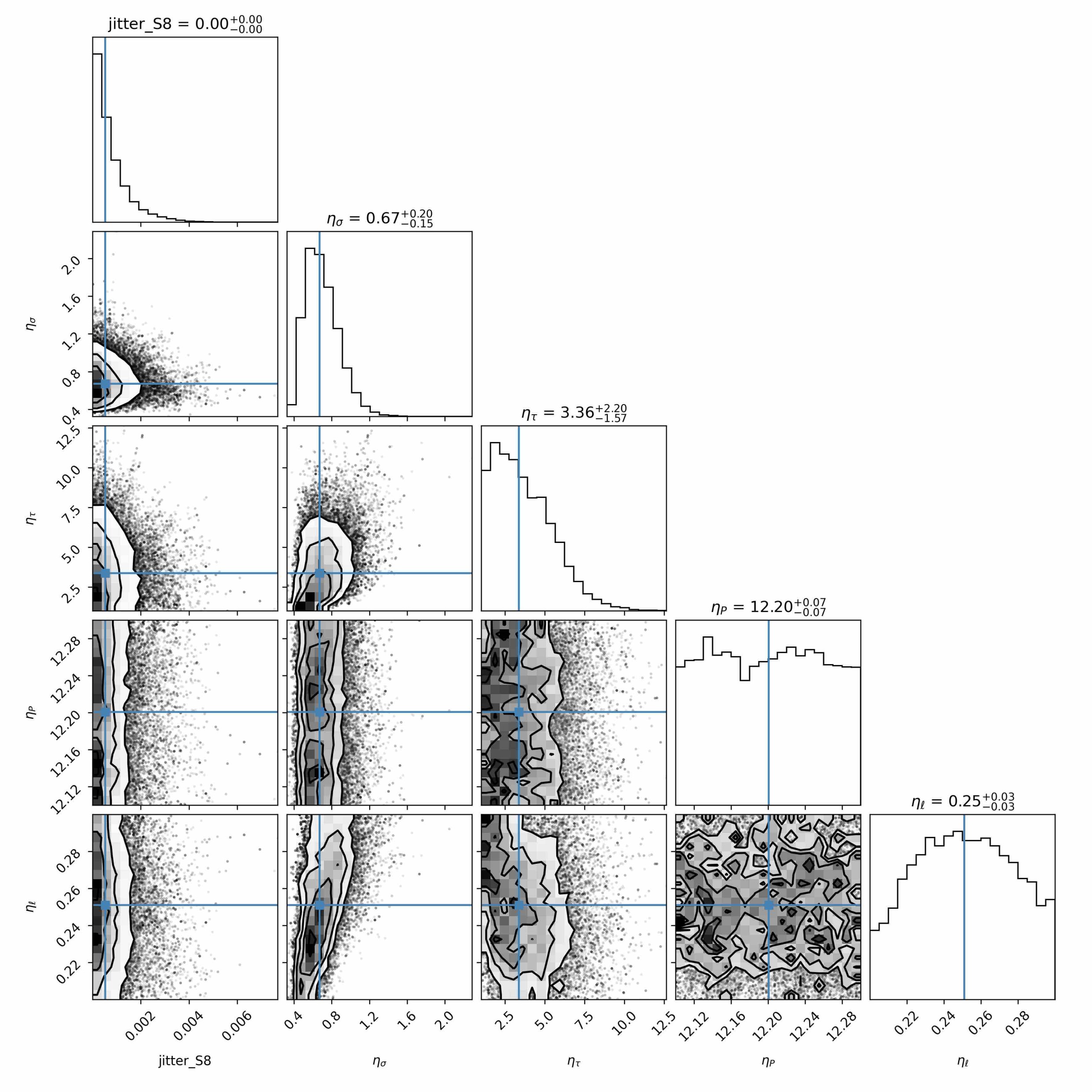
We first apply our GP model to the SuperWASP data for the 4 seasons together (Figure 3). We use wide uniform priors on hyper-parameters , and . Instead of accounting for intrinsic uncertainties in the light curve, we also fit a jitter term . For the hyper parameter , we use a prior of based on periodogram analysis of the WASP light curves in 3.1.3. We recover from the MCMC of the WASP data spot lifetime of 57.96 days, a rotation period of of 12.03 days, and a smoothing hyper-parameter which are consistent with our young star and such long spot lifetimes are seen for other young systems (Figure 10, e.g., Cale et al., 2021). We adopt these three posteriors as priors in constraining the GP model for our RV stellar activity analysis.
We next analyze both Sectors of TESS PDC-SAP and SAP separately in order to see if we can recover similar GP kernel hyper parameters to our SuperWASP analysis. We first median normalize the TESS SAP light curve, mask out the transits, and the edges of the light curve data, particularly for Sector 8 where there exists a spacecraft systematic producing a “ramp-up” effect at the start of the sector and after the data downlink gap mid-sector. We then fit the remaining light curve via a cubic spline regression (scipy.interpolate.LSQUnivariateSpline; Virtanen et al. (2020)) for each Sector individually with knots sampled in units of 1.3 days (excluding any that happen to fall within the TESS data dump regions). The particular value of 1.3 is chosen to be small with respect to the stellar activity time-scales, but long with respect to the cadence, so transits are “smoothed” over to produce a “noiseless” and smooth representation of the light curves. Then, in Figure 9 we apply the technique (Aigrain et al., 2012) to the spline regression fits.
We used a uniform prior centered on 12.2 days for the stellar rotation period hyper-parameter. As expected due to the relatively short TESS time baselines of two 13-day observing sequences per sector, the TESS light curve does not constrain the stellar rotation period further than the information inferred from the SuperWASP light curve analysis.
For TESS SAP sector 8 (34; 8+34) light curve we recover from the MCMC a spot lifetime of 12.94 (10.10 days; 15.97) days. In other words, the TESS light curve analysis leads to a significantly shorter spot life-time analysis than inferred from the SuperWASP analysis as well, even for the SAP fluxes, but we discard these results as a consequence of the shorter TESS time baseline compared to the SuperWASP light curve, even though the former is at higher photometric precision. For TESS SAP sector 8 (34; 8+34) light curve we recover from the MCMC a smoothing hyper-parameter (;), and these are all somewhat smaller than the value inferred from the SuperWASP analysis, and this could potentially be due to the higher precision of the TESS light curves and improved photometric sampling of the rotation period. Finally, from a MCMC of the TESS PDC-SAP light curves, we recover even shorter spot lifetime , indicating that the pre-search data conditioning (PDC) can lead to introducing systematics that lead to inaccurate characterization of the stellar activity (Figure 12).
3.2.4 ExoFAST
In this section, we perform an EXOFASTv2 analysis of the candidate planets transit light curves. After normalizing the TESS PDC-SAP data as described in section 2, we cut out a region of at least 8 hours around each individual transit and create separate data files for each transit and use these as input data for EXOFASTv2.
We jointly model the TESS, Spitzer and ground-based light curves, and all RVs with EXOFASTv2. The EXOFASTv2 RV results are presented in the Appendix in Figure 41. However, while ExoFAST can jointly model the light curves and RVs, the EXOFASTv2 RV model does not account for the stellar activity manifested in the RV measurements. Thus, we perform an independent modeling of the RVs with a stellar activity model in 3.3.
Our minimal set of priors are detailed in Table 5, including the period P, time of conjunction, and planetary radius for TOI 560 b and c (the EXOFASTv2 full results are in Table 7). We allow other model parameters, i.e. eccentricity , inclination , and argument of periastron to vary with no imposed priors, starting with circular and edge-on values. The posterior values for this initial MCMC run are then used as the initial values for a second iteration run, though we keep the same uniform and Gaussian priors as the initial run. We allow this second run to run longer, and we confirm the second MCMC converges on the same results within 1 to check for the robustness of the MCMC posteriors. Note that the model is parameterized in the EXOFASTv2 standard basis for transit only fits. This model parameterization is (Eastman et al., 2019).
| Parameter | Initial | Priors |
| value | ||
| [] | ||
| Pb [days] | 6.3981 | |
| TCb [days] | 2458517.69007 | |
| Pc[days] | 18.881 | |
| TCc[days] | 2458533.59092 | |
| 0.0388 | – | |
| 0.0382 | – | |
| 0.000030 | – | |
| 0.000030 | – | |
| 0.674 | – | |
| 0.679 | – | |
| [K] | 4599.94 | – |
| [K] | 4591.85 | – |
| feh | -0.031 | |
| initfeh | -0.043 | – |
| eep | 319.8 | – |
| log | -0.145 | – |
| 0.097 | ||
| errscale | 1.22 | – |
| distance [pc] | 31.567 | – |
are assumed to be circular, with no priors.
3.3 RV Analysis
In this section, we jointly analyze our RVs (Table 15) from three spectrographs (iSHELL, PFS, and HIRES). We analyze the RVs as a planetary system with a chromatic GP stellar activity model, and make model comparisons. We constrain our GP model hyper-parameters from the SuperWASP light curve analysis, in particular the stellar rotation period and spot lifetime timescale.
3.3.1 Planet System Multi-Spectrograph RV Analysis
To jointly model the RVs from iSHELL, PFS and HIRES, we again use pychell, this time in combination with the co-dependent package optimize, which is a general-purpose Bayesian analysis tool that pychell expands upon with RV-specific MCMC tools. In Section (5.2) we show that no statistically significant periodic signals were identified in the raw RVs, and so we proceed herein with the assumption of a two planet model in our Bayesian analysis with the ephemerides from TESS. Each planet in our model consists of five parameters, which comprise a complete orbit basis: the period , time of conjunction , eccentricity , argument of periastron , and RV semiamplitude , with subscripts denoting the planet said parameter is associated with (in this case, b and c). We next include a GP model for the stellar activity, which is described further in the next sub-section. We also include an absolute RV offset term () to account for the average overall recessional velocity of the star, and a jitter term () which quantifies the variational RV amplitude not accounted for by any modeled planets, stellar activity, or instrumental noise that is non-frequency dependent on our time-scales of interest (e.g. white noise). Analyses of the PDC-SAP TESS transit data (Section 4.1.1 - Figure 13 and Table 5) shows a period and time of conjunction consistent with those listed on the ExoFOP-TESS database in the TESS Object of Interest (TESS Project section)121212https://exofop.ipac.caltech.edu/tess/target.php?id=101011575 (Akeson et al., 2013) which are days, , days and , all of which have an uncertainty which are orders of magnitude finer than we can hope to resolve with our RV cadence. We thus decide to lock both parameters at their nominal values for all analyses in this paper. For all MCMC results quoted, the median value is defined as the 50th percentile, while the lower and upper uncertainty bounds are the 15.9th and 84.1th percentile posterior confidence intervals, respectively. We sample the posterior distributions using the emcee package (Foreman-Mackey et al., 2013) for a subset of models to determine parameter uncertainties, always starting from the MAP-derived parameters (i.e. affine invariant is our actual sampler. We perform a burn-in phase of 1000 steps followed by a MCMC analysis for approximately fifty times the median auto-correlation time (steps) of all chains. The prior, posterior distributions, and results of this model is in section 4. Finally, we also perform a model comparison test (Table 9) by calculating the , small-sample Akaike Information Criterion (AIC; Akaike, 1974; Burnham & Anderson, 2002), and Bayesian Information Criterion (BIC) for each combination of planets in our model. These results are shown in Section 4.2.
| Parameter [units] | Initial Value () | Priors | MAP Value | MCMC Posterior |
| [days] | 6.3980661 | \faLock | – | – |
| [days] | 2458517.68971 | \faLock | – | – |
| 0.294 | ; | 0.0.33 | ||
| ; | 4.11 | |||
| [m s-1] | 10 | 6.57 | ||
| [days] | 18.8805 | \faLock | – | – |
| [days] | 2458533.593 | \faLock | – | – |
| 0.093 | ; | 0.19 | ||
| ; | -3.87 | |||
| [m s-1] | 10 | 6.80 | ||
| [m s-1] | 4.22 | |||
| [m s-1] | -13.28 | - | ||
| [m s-1] | 4.59 | |||
| 12.03 | 12.02 | |||
| 0.44 | \faLock | – | – | |
| 57.96 | \faLock | – | – | |
| 1 | 23.42 | |||
| 1.17 | 0.61 |
. \faLock indicates the parameter is fixed. Gaussian priors are denoted by , uniform priors by lower bound, upper bound, and Jeffrey’s priors by lower bound, upper bound. The on the initial gamma values are in case the RVs are already median-subtracted, and to pseudo-randomize this initial parameter.
a We want the initial value to be the median of the RVs for that spectrograph; the is used incase the median is already zero, as Nelder-Mead solvers cannot start at zero.
3.3.2 Stellar Activity RV Model - RVs
Rather than applying an independent GP model to each individual RV data set for PFS, HIRES and iSHELL, we extend the kernel in Equation 1 to utilize a single global (joint) GP model and covariance kernel across multiple spectrographs. We follow Cale et al. (2021) where they already implemented our desired framework in two Python packages. As in Cale et al. (2021), we first re-parametrize the GP amplitude through a linear kernel, hereafter referred to as the kernel as in Cale et al. (2021) as follows:
| (3) |
Here, , are the effective stellar activity amplitudes for each spectrograph at times and , respectively, where represents an indexing set between the observations at time 131313Truly simultaneous measurements with identical mid-point exposure times, i.e., = , would necessitate a more sophisticated indexing set.. In the kernel each instrument is given its own independent amplitude hyper-parameter, , but the other three hyper-parameters are shared between all instruments. Also, the covariance kernel is still square, but now has dimensions corresponding to the total number of observations across all spectrographs, and thus represents a “joint” covariance matrix.
Second, to first order, we expect the amplitude from stellar activity to be linearly proportional to frequency (or inversely proportional to wavelength) (Cale et al., 2021). This approximation is a direct result of the spot-contrast scaling with the photon frequency (or inversely with wavelength) from the ratio of two black-body functions with different effective temperatures (Reiners et al., 2010). Thus, we also consider a variation of this kernel which further enforces the expected inverse relationship between the amplitude with wavelength. As in Cale et al. (2021) we parametrize the kernel to become:
| (4) |
which hereafter we refer to as the kernel as in Cale et al. (2021). Here, is the effective amplitude at , and is an additional power-law scaling parameter with wavelength to allow for a more flexible non-linear (with frequency) relation. and are the “effective” wavelengths for observations at times and , respectively. Note for this kernel, we are ignoring the chromatic effects of limb-darkening and convective blueshifts on the RVs which will impact the covariance matrix; however given the flexibility of the GPs, Cale et al. (2021) finds this chromatic kernel effectively recovers the wavelength dependence of stellar activity induced RV variations. For both eqs. (3) and (4), the expression within square brackets is identical to that in eq. (2).
We apply Kernels and to our RV data, using the priors in Table 6, the priors from our FF analysis in 3.2.3 for the model hyper-parameters, as well as a set of disjoint quasi-periodic kernels as in Equation 1, one GP for each spectrograph akin to RadVel (Fulton et al., 2018). In the analysis presented herein we fix and to the median values from the SuperWASP light curve analysis posteriors; letting these model hyper-parameters vary in our RV analysis – with prior minimums of 0.2 and 20 days respectively – yields quantitatively identical results for the median posterior values for and , albeit with slightly larger confidence intervals. We also analyze the RVs using no GP, effectively assuming the stellar activity is not present.
4 Results
In 4.1, we present the transit analyses of the TESS, Spitzer and ground-based light curves using EXOFASTv2. Then in 4.2 we present the RV analysis with pychell and the GP stellar activity model.
4.1 Transit Light Curves
In this subsection we represent the results of our ExoFASTv2 analysis of the light curves and vetting results.
4.1.1 TESS Light Curves
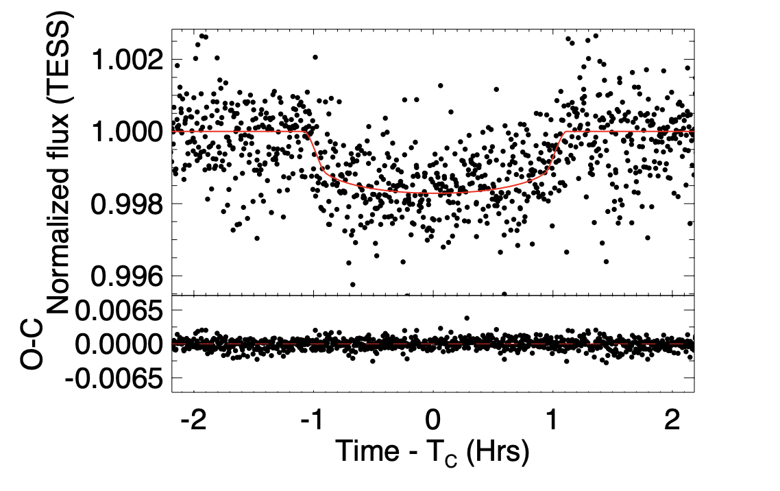
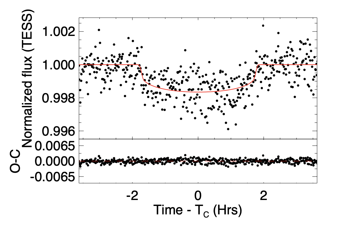
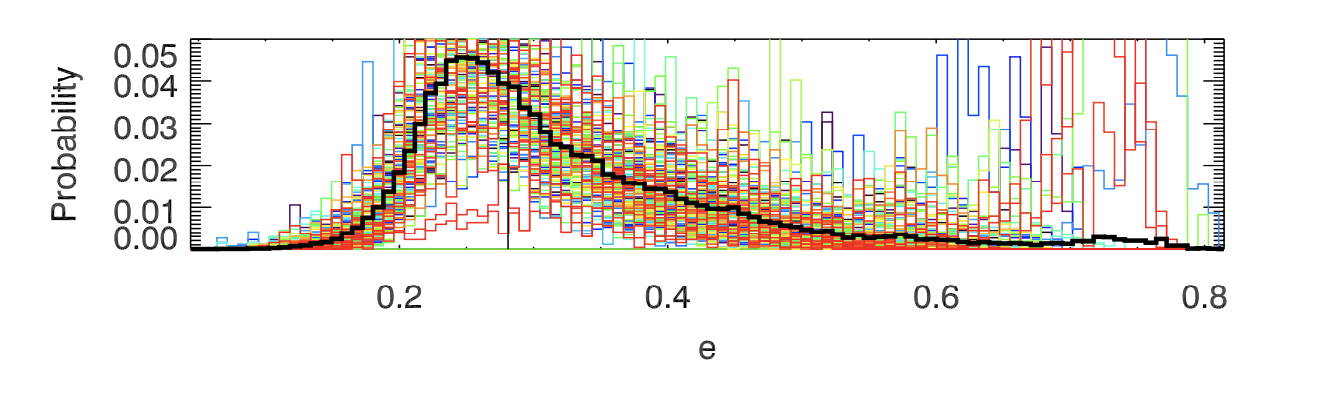
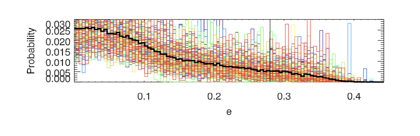
The TOI 560 TESS light curves for Sectors 8 and 34 are shown in Figure 13, after subtracting off a cubic-spline regression fit for the out-of-transit stellar activity from the PDC-SAP light curves shown in Figure 9. The ExoFASTv2 analysis reveals clear transits of TOI 560 b and c with expected depths and transit times consistent with the TESS mission TOI 560 b and 560.02 candidates. Table 7 shows the median and confidence intervals for the model and derived planetary parameters. Figure 14 shows the phased TESS transits. Of particular note, we confirm a non-zero eccentricity for TOI 560 b at 4.7-; the eccentricity posterior for TOI 560 c is consistent with zero (Figure 15). The statistical significance of the non-zero eccentricity detection for TOI 560 b is primarily driven by the photo-eccentric effect using the Spitzer data (Dawson & Johnson, 2012), as excluding this particular data set decreases the statistical significance on to , but still with a similar non-zero median eccentricity. Finally, the Spitzer light curve is presented in 4.1.2, ground-based PEST, NGTS, and LCO light curves are presented in the Appendix.
| Planetary Parameter | Units | Planet b | Planet c |
|---|---|---|---|
| P | Period (days) | ||
| RP | Radius (RJ) | ||
| RP | Radius (RNep) | ||
| RP | Radius (R⊕) | ||
| Tc | Time of conjunctiona (BJDTDB) | ||
| TT | Time of minimum projected separationb (BJDTDB ) | ||
| T0 | Optimal conjunction Timec (BJDTDB) | ||
| Semi-major axis (AU) | |||
| Inclination (Degrees) | |||
| Eccentricity | |||
| Argument of Periastron (Degrees) | |||
| Teq | Equilibrium temperatured (K) | ||
| Tidal circularization timescale (Gyr) | |||
| RVsemi-amplitude(m/s)e | |||
| Radius of planet in stellar radii | |||
| Semi-major axis in stellar radii | |||
| Transit depth in B (fraction) | |||
| Transit depth in R (fraction) | |||
| Transit depth in z’ (fraction) | |||
| Transit depth in 4.5 m (fraction) | |||
| Transit depth in TESS (fraction) | |||
| Ingress/egress transit duration (days) | |||
| Total transit duration (days) | |||
| FWHM transit duration (days) | |||
| Transit Impact parameter | |||
| Eclipse impact parameter | |||
| Ingress/egress eclipse duration (days) | |||
| Total eclipse duration (days) | |||
| FWHM eclipse duration (days) | |||
| Blackbody eclipse depth at (ppm) | |||
| Blackbody eclipse depth at (ppm) | |||
| Blackbody eclipse depth at | |||
| Incident Flux ( erg s-1 m-2) | |||
| Time of Periastron (BJDTDB) | |||
| Time of eclipse(BJDTDB) | |||
| Time of Ascending Node(BJDTDB) | |||
| Time of Descending Node (BJDTDB) | |||
| Equivalent Circular to Measured Eccentric Velocity ratio | |||
| Eccentricity times Cosine of the Periastron Angle | |||
| Eccentricity times Sine of the Periastron Angle | |||
| Separation at mid transit | |||
| A priori non-grazing transit prob | |||
| A priori transit prob | |||
| A priori non-grazing eclipse prob | |||
| A priori eclipse prob |
a Time of conjunction is commonly reported as the ”transit time”. b Time of minimum projected separation is a more correct ”transit time”. c Optimal time of conjunction minimizes the covariance between TC and Period. d Assumes no albedo and perfect redistribution. e The recovered semi-amplitudes for the planets in the ExoFASTv2 analysis are significantly smaller than the those recovered in Table 6 with our RV analysis that includes a stellar activity model, and thus would appear at first to be contradictory. However, they are not statistically significant detections in this ExoFASTv2 analysis, as the posteriors are peaked at 0 m/s, and the reported confidence intervals herein are consequently misleading. The corresponding 5- upper-limits are 15 and 10 m/s for and respectively.
4.1.2 Spitzer Light Curve
The Spitzer light curve (Figure 16) shows a transit that is consistent with the expected timing, duration and depth from TESSfor TOI 560 b. This helps rule out false positive eclipsing binary scenarios due to the lack of any observed chromaticity in the depth and shape of the observed transit. Additionally, the Spitzer light curve is at higher photometric precision and temporal sampling with respect to TESSgiven the larger aperture of Spitzer; there is less limb-darkening compared to visible wavelengths, and less photometric variations due to stellar activity. Therefore these observations help further constrain the exoplanet parameters of TOI 560 b and refine the orbital ephemerides. In particular, the Spitzer light curve enables us to detect the eccentricity of TOI 506 b via the photo-eccentric effect as deviating from zero at 4.7. This eccentricity is marginally detected in the TESS transits, but is not statistically significant without the Spitzer observations.
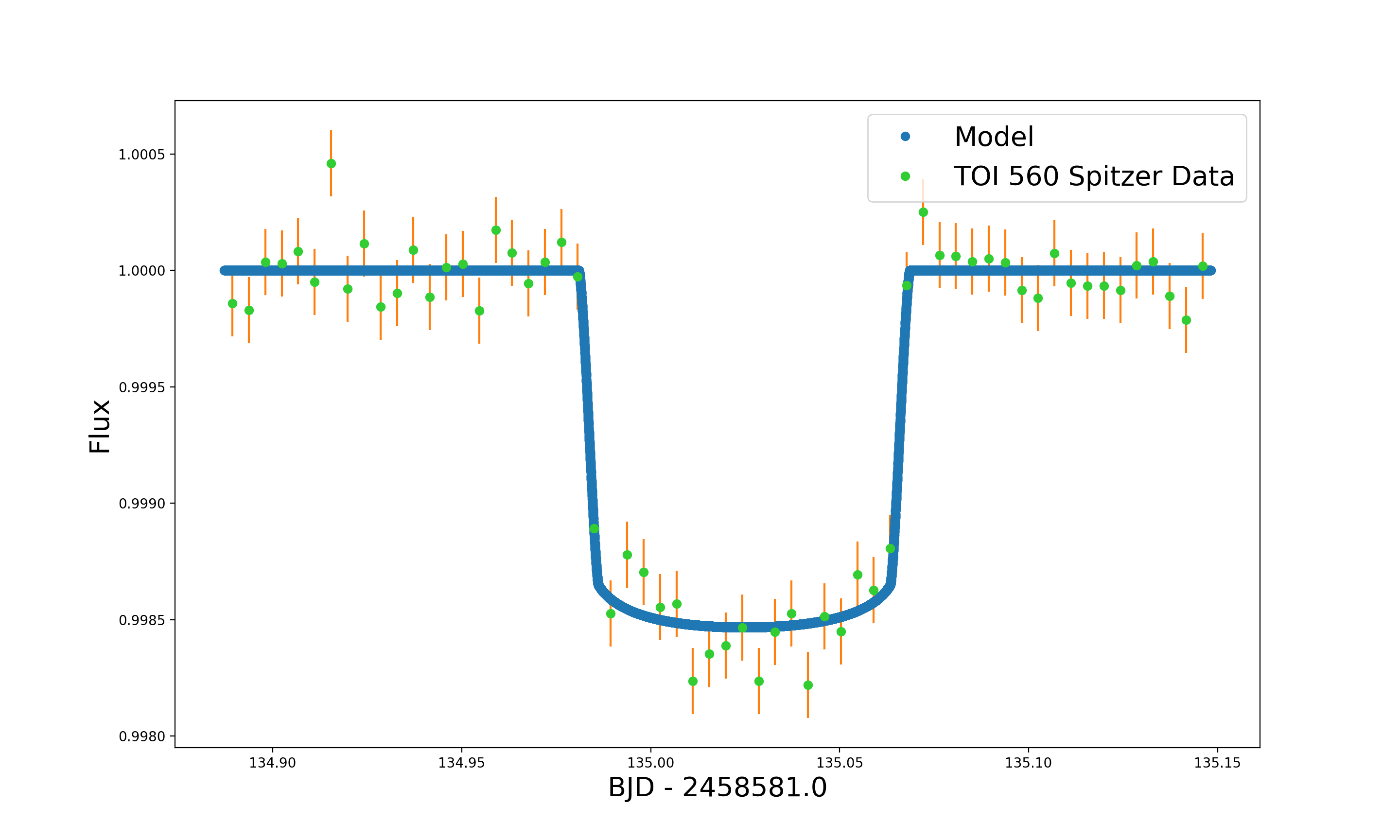
in blue.
4.2 RV pychell Results
Using our RV model with pychell we produce consistent and stable MCMC results for all GP kernels considered that provide detections for the masses of TOI 560 b and c, establishing their nature as a pair of Neptune-mass exoplanets consistent with their radii (Table 6). For our adopted final result using the kernel, the RV models with MAP values and MCMC cornerplot are shown in Figures 17, 18, and 19. The best MAP fit, and MCMC median and confidence intervals are presented in Table 6. The table of exoplanet mass and density measurements are derived from our RV analysis are in Table 8. In the Appendix in Figure 25, we present the mass-radius diagram for known transiting exoplanets with measured masses (Akeson et al., 2013), with the detections for TOI 560 b and c shown to be consistent with the older Neptune-mass regime.
We present in the Appendix the results of the RV analyses for the joint GP kernel, the disjoint “classsic” quasi-period GP kernel where there is a separate GP for every spectrograph, and for the RV analysis with no stellar activity assumed in Tables 13 and 14 respectively. All yield similar detections or upper-limits to the exoplanet velocity semi-amplitudes and consistent model hyper-parameters for the stellar activity.
A model comparison in Table 9 shows that the RVs support the detection of both planets b and c combined and also planets b and c individually. The 1 and 2 planet models are statistically indistinguishable. The no-planet scenario is ruled out. Additionally, we do recover () detections of TOI 560 b (c) with our kernel. For the other kernels presented in the Appendix, we find qualitatively similar marginal and 3- recoveries of and/or . Our kernel model estimates the masses of planets b and c to be and .
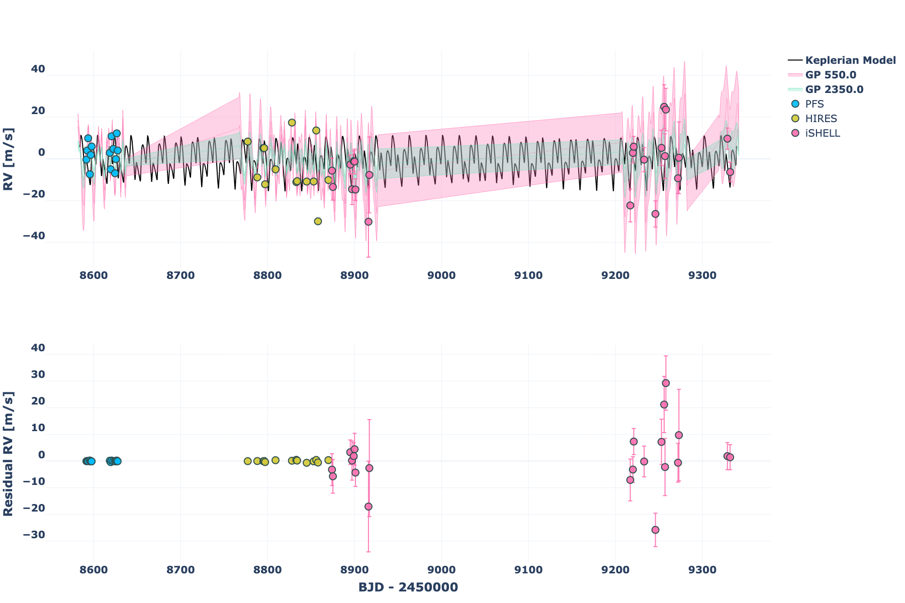
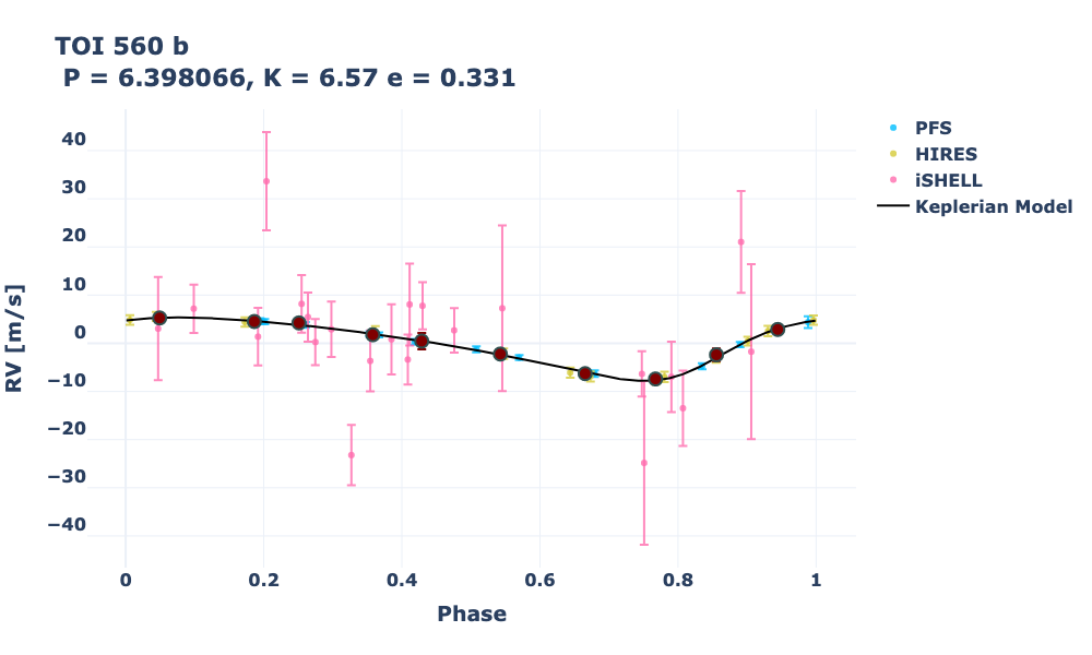
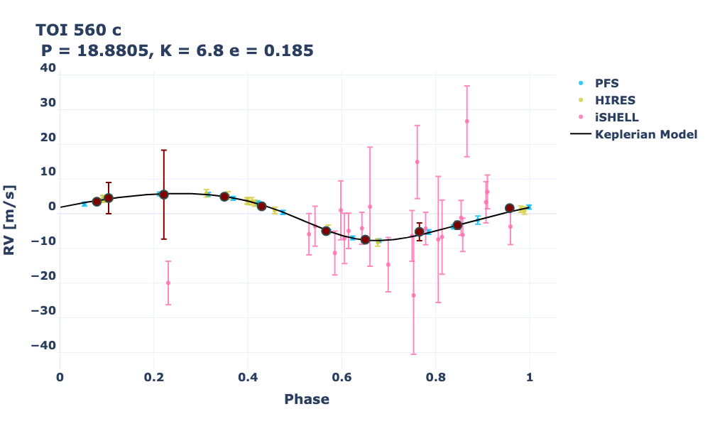
. The best fit MAP Keplerian model is shown as the black curve, with a fixed circular orbit, velocity semi-amplitude , and orbital period indicated.
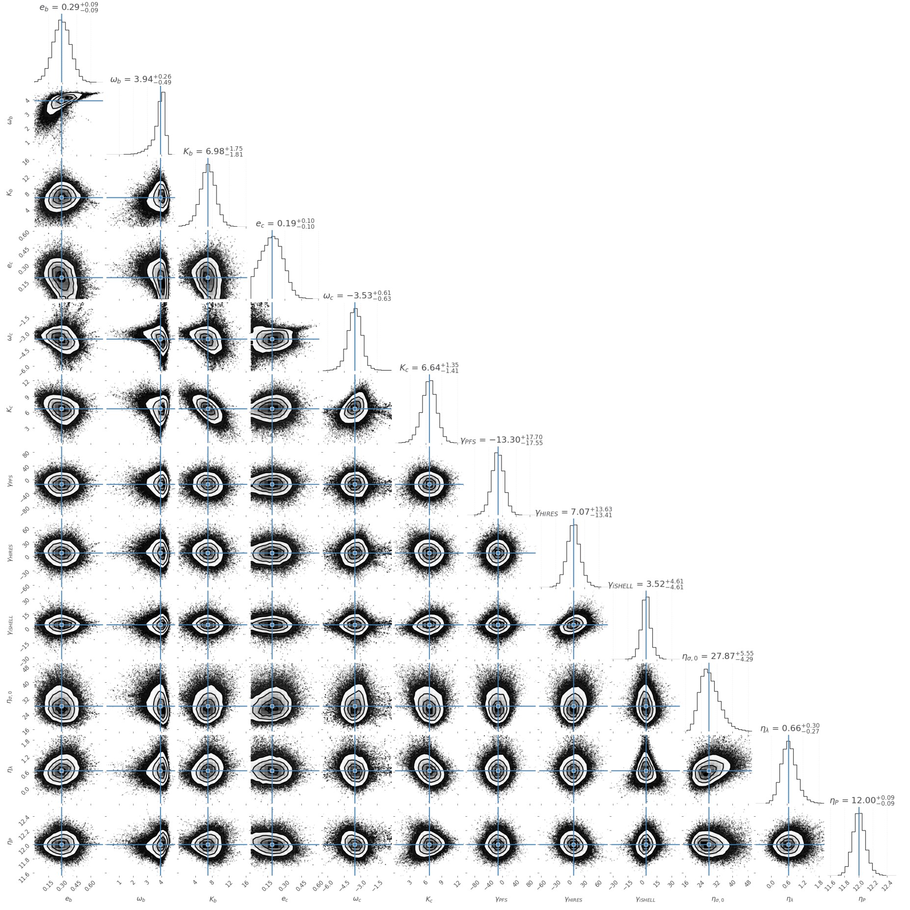
| Planet | Mass | Density (gcm-3) |
|---|---|---|
| b | M⊕, MNep | |
| c | M⊕, MNep |
| Planets | AICc | BIC | N free | ||
|---|---|---|---|---|---|
| b, c | -197.0 | 0.0 | 1.5 | 12 | 1.1 |
| b | -202.1 | 0.3 | 0.0 | 9 | 0.9 |
| c | -204.5 | 5.1 | 4.7 | 9 | 0.9 |
| None | -233.9 | 55.3 | 51.7 | 6 | 1.4 |
5 Discussion
In the previous sections we have validated the presence of a two-planet system orbiting a young, 600 Myr host star TOI 560, detected the individual planet masses at , establishing the planets as Neptune analogs. In this discussion, in 5.1, we present a dynamical stability analysis of the system, which appear stable over the 10 Myr timescale explored. Next we consider the near 1:3 orbital resonance of TOI 560 b and c, and what implications that may have for additional planets and formation in 5.3. Finally, in 5.4 we discuss the suitability of the TOI 560 system for future atmospheric characterization.
5.1 Dynamical Stability: Two-planet REBOUND Simulation
We perform dynamical stability tests of the TOI 560 system over a duration of 10 Myr using REBOUND, an N-body gravitational integrator built in C and usable in python (Rein & Liu, 2012a; Rein & Spiegel, 2015a). To define each orbit, we use the , , eccentricity, and inclination median values from our EXOFASTv2 MCMC analysis in Table 7, and we use the median planet masses from our J2 kernel model values from Table 8. We choose an integration time-step shorter than of the shortest orbital period ( days). The results of this dynamical simulation are shown in Figures 20 and 21. The simulations show the dynamical interactions between TOI 560 b and c, with a mean motion resonant libration precession of the longitudes of periastron. This demonstrates that the detected eccentricity for TOI 560 b could be a consequence of the dynamical interaction with TOI 560 c. The orbits of both planets are stable and possessing moderate eccentricities over the entire 10 Myr simulation duration. We did not run the simulation to 1 Gyr, the estimated lifetime of the system, because of the near 1:3 orbital resonance; a mean-motion orbital resonance (MMR) can either stabilize or destabilize the system within a timescale of a few hundred orbits, so if the system was unstable, the instability would have been apparent in the simulation well within a few Myr.
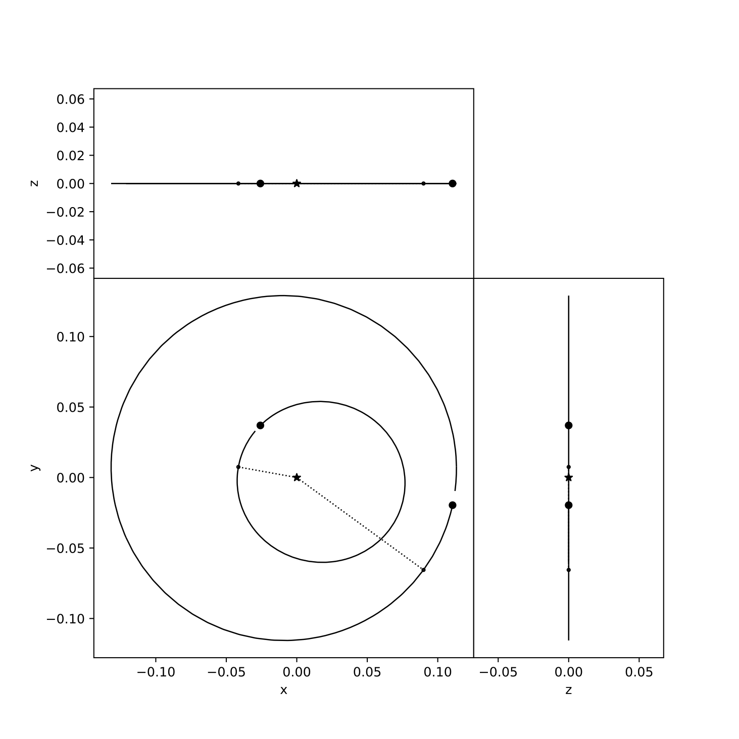
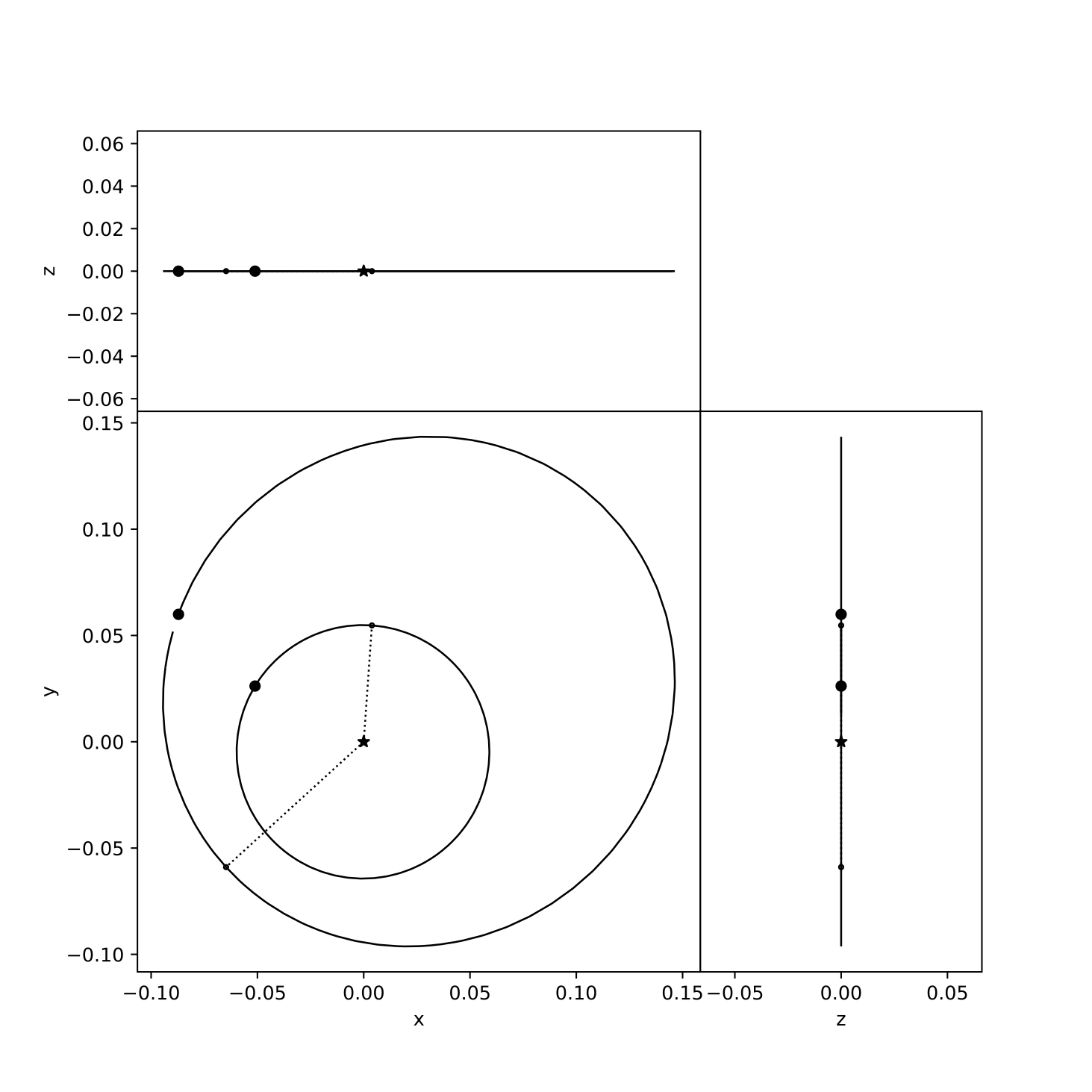
orbital configurations of our two-planet model in REBOUND with inclination estimated from EXOFASTv2. The , and axes are in AU. The planet positions are noted as black dots, and the orbits as circles. The periastron vectors are marked with dashed lines starting from the star (star symbol) at the origin of the orbits, and show significant evolution from the start to the beginning of the simulation.
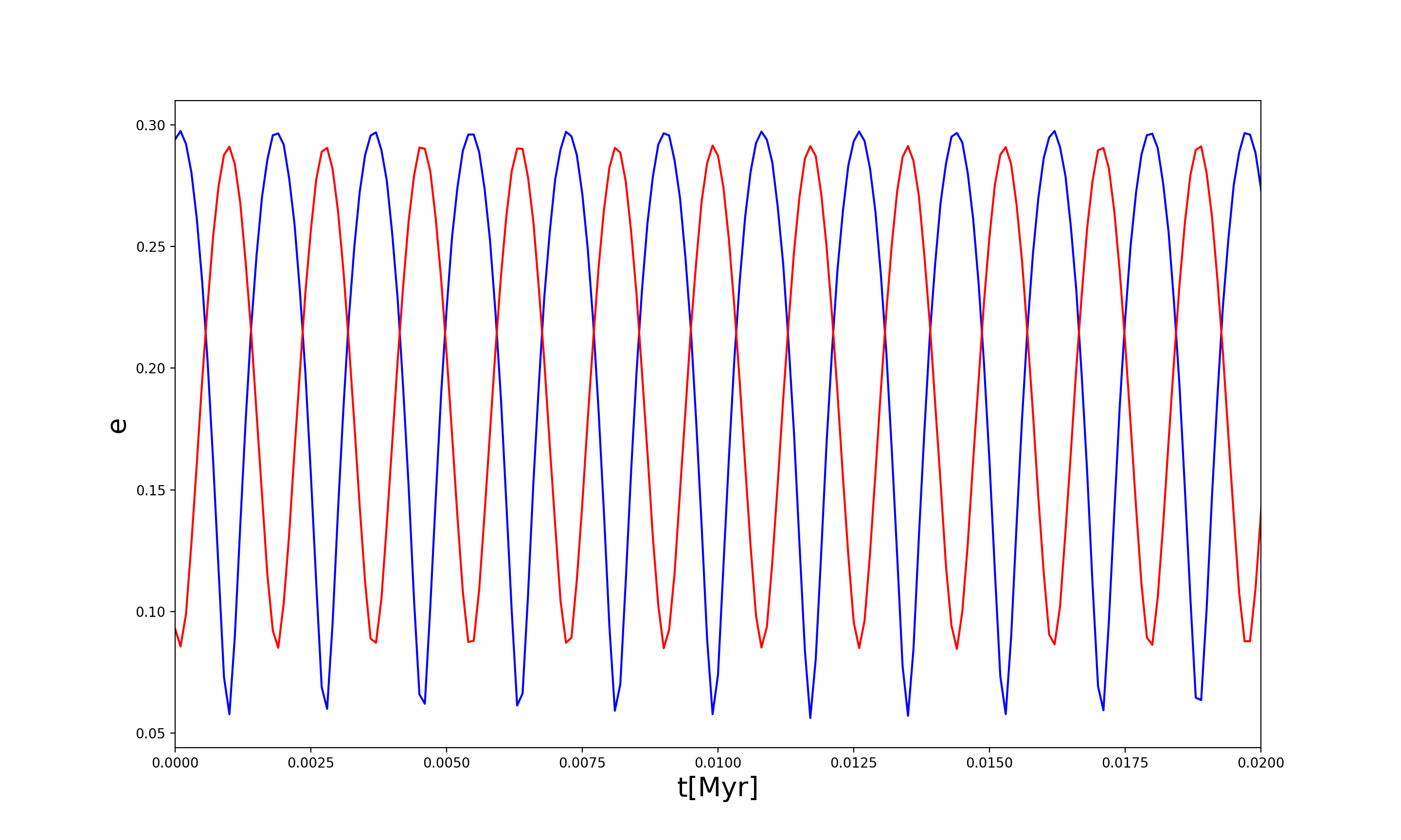
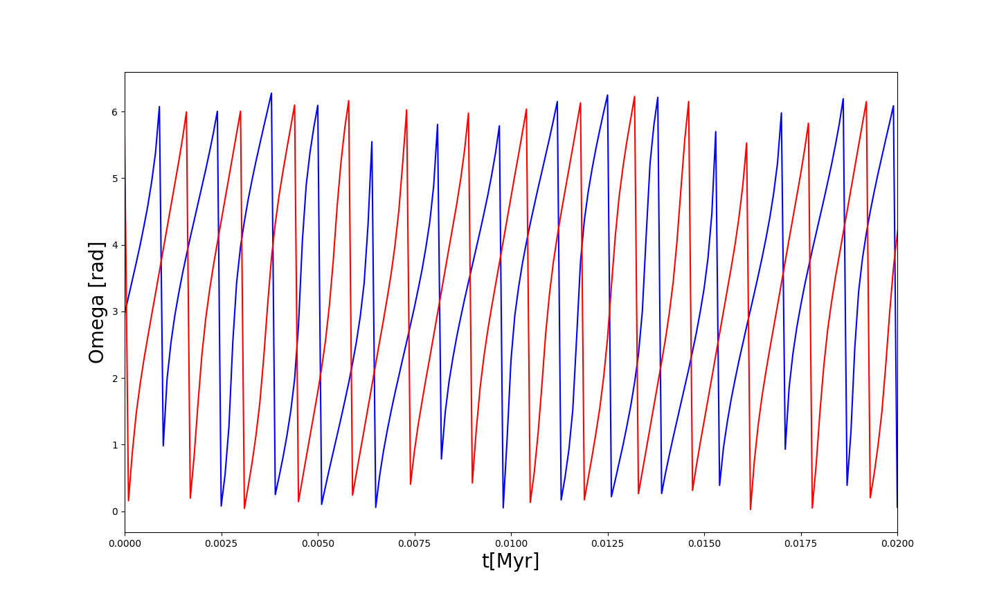
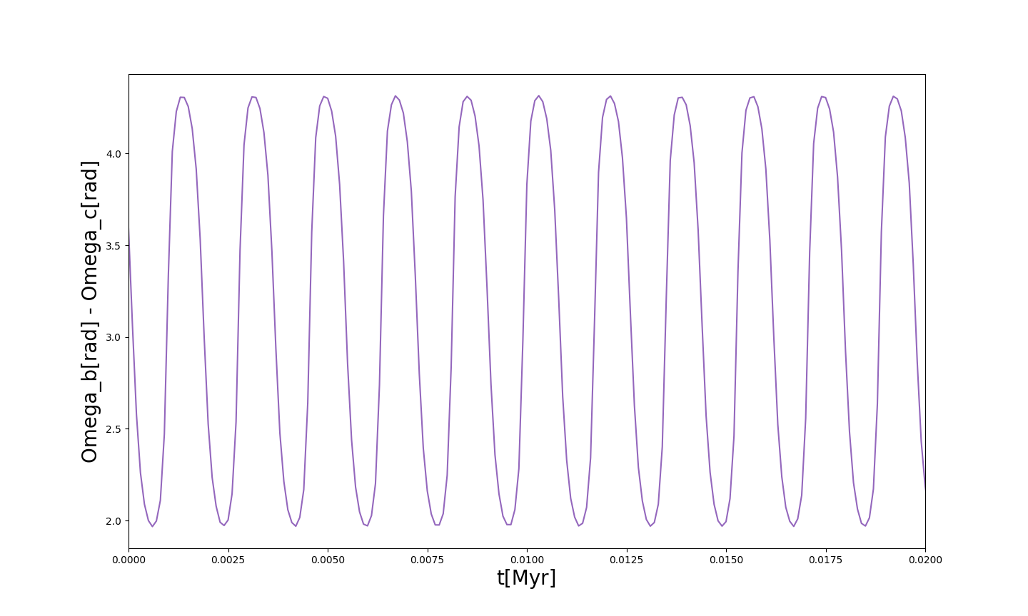
5.2 The Search for Additional Candidates
Fourier-like periodograms can be useful in determining prominent frequencies in unevenly sampled RV time-series. First, we calculate Generalized Lomb-Scargle (GLS) (Zechmeister & Kürster 2009; Scargle 1982) periodograms. The GLS periodogram power at a given trial period directly correlates with the Keplerian velocity semi-amplitude of a circular-orbit planet signal at that trial period. Multiple periodic signals are identified by subtracting a best-fit periodic signal from the data, and then repeating the periodogram calculation on the residuals; this process is repeated until no more statistically significant signals are identified.
For TOI 560 in particular, we compute a GLS periodogram utilizing a stellar activity + two planet model for b and c. We first remove the nominal GP and zero-points; this periodogram is used to see if we can identify the RV signal of b or c, or any additional planet(s) present in the system as a periodogram peak. Then we further remove best-fit RV signal for TOI 560 b, and re-compute the periodogram; this periodogram is used to see if we can identify the RV signal of TOI 560 c or any additional planet(s) present in the system. Third, subtract off the best fit model for planet c, and re-compute the periodogram of the residuals; this periodogram is used to search for any additional planets in the system. In all cases, the orbital period and time of conjunction and thus orbital phase of either TOI 560 b and/or c are fixed in fitting the planet signals to the RV time-series data, and only the velocity-semi-amplitude, eccentricity, and angle of periastron are free (fitted) parameters. We calculate false-alarm probabilities using both the standard analytic formula derived from the periodogram power (Zechmeister & Kürster 2009; Scargle 1982), and empirically through a 1000-trial bootstrap process of: scrambling (re-ordering) the times of observations while holding the ordering of the RV values fixed (or conversely, scrambling the ordering of the RV values while holding the ordering of the times of observations fixed), then recomputing the periodogram, and then investigating the empirical distribution of the top power values. While GLS periodograms have historically been successful in identifying genuine multi-planet signals in RV time-series data, this approach is also fraught with the identification of false positive signals because of the overly simplistic assumptions (e.g., Robertson et al., 2014, 2015); it can be difficult to discern whether GLS periodogram peaks are real planet signals, or some form of systematic red noise (e.g. a cadence alias, imperfect signal subtraction in the iterated residuals, stellar rotational modulation of activity, etc. Vanderburg et al., 2016a; Dawson & Fabrycky, 2010). We also compute the window function of the RV time-series by setting all RV values equal to zero and computing a Lomb-Scargle periodogram to identify any periodogram peaks that are associated with temporal sampling cadence aliases, such as integer fraction multiples of one day or one year.
Second, Bayesian model-based periodograms enable statistically-robust comparisons that jointly capture the full model complexity of potentially multi-planet systems with models for stellar activity embedded in the noisy, unevenly sampled RVs (e.g., Anglada-Escudé et al., 2016; Tuomi et al., 2014). First, we compute a maximum-likelihood fit to the RVs for a model with stellar activity and a first “trial” planet of unknown phase and velocity semi-amplitude at a trial orbital period. We follow the same implementation as in Cale et al. (2021). We compute this one-planet model over a set of trial periods to generate the first periodogram, which is used to see if we can identify the RV signal of b or c, or any additional planet present in the system as a periodogram peak. Second, we add to our model a planet at the orbital period and time of conjunction of TOI 560 b, in addition to the trial planet. We compute maximum-likelihood fits to this two-planet model over the same set of trial periods to compute the second periodogram, which is used to see if we can identify the RV signal of TOI 560 c, or any additional planet present in the system as a periodogram peak. Third, we add to our model a third planet at the orbital period and time of conjunction of TOI 560 c to see if we can identify the RV signal for any additional planet present in the system besides TOI 560 b or c.
The GLS periodograms are shown in Figure 22, and the periodograms are shown in Figure 23. We find two periodogram peaks that are persistent with a 15 at 4.57 and 5.54 days, particularly for the periodograms where TOI 560 b is included in the model. The 5.54 day period would likely not be dynamically stable with the TOI 560 b at 6.40 days. However, the 4.57 periodogram peak suggests a possible non-transiting candidate that would be near a 2:3 orbital resonance with TOI 560 b. This period is also not near an alias of the stellar rotation period. Furthermore, the 5.54 day peak is close to the frequency difference between the 4.57 day peak and the cadence alias of 5 days and is thus potentially a cadence alias of the 4.57 day peak. Consequently, we perform a model comparison with a third non-transiting interior planet at this orbital period of 4.57 days. However, the model comparison disfavors the detection of this planet. Thus our existing data is insufficient to confirm the possibility of an additional non-transiting candidate planet in this system.
5.3 Implication of the near 1:3 orbital period resonance of TOI 560 b and c
Given the youth of TOI 560, neither planet would have been tidally circularized by the star if they started with an initial high eccentricity formation mechanism (Rasio et al., 1996; Bodenheimer et al., 2003). Our RVs are not sufficient to constrain the eccentricities of either planet, given that we have only a marginal mass detection of TOI 560 b and a non-detection of TOI 560 c, and also due to the presence of the stellar activity. However, our ExoFASTv2 analysis of the TESS Spitzer and ground transits of TOI 560 b confirms a moderate eccentricity of 0.29 (Figure 15). Both planets show that a high eccentricity is disfavored. This implies that TOI 560 b and c likely did not form in a high-eccentricity migration scenario, and more likely formed in-situ, unless the migration took place when a significant gas disk was still present to dampen the orbital eccentricities (Plavchan & Bilinski, 2013; Lin et al., 1996; Ward, 1997). The orbital eccentricity of TOI 560 b will be an important parameter to further constrain with future observations, such as may be possible with secondary eclipse observations and additional high precision RVs.
The orbital period near-commensurability of TOI 560 b and c to a 1:3 ratio also has interesting implications for planet formation. For one, such an orbital resonance is rare among mature exoplanet systems identified by Kepler (Figure 4, Fabrycky et al., 2014). Far more common among mature compact multi-exoplanet systems are the 2:3 and 1:2 near-commensurability orbital period resonances. This raises the interesting possibility that there could be a third middle planet in the TOI 560 system that is non-transiting with an orbital period of 12.6 days that would establish the TOI 560 system in a 1:2:3 orbital resonant chain at an age of 1.5 Gyr. Such systems of transiting exoplanet systems orbiting mature stars with middle non-transiting companions are more common than perceived – e.g. Christiansen et al. (2017), Buchhave et al. (2016), Sun et al. (2019), and Osborn et al. (2021) identified similar exoplanet configurations for the HD 3167, Kepler-20, Kepler-411, and TOI-431 planetary systems respectively.
The 22 Myr AU Mic system is possibly also in a resonant 4:6:9 orbital chain with a middle non-transiting planet candidate (Cale et al., 2021; Wittrock et al., 2022), and the 20 Myr v1298 Tau system is in a 2:3:6:10 resonant chain (David et al., 2019a; Feinstein et al., 2021; Suárez Mascareño et al., 2021). Similarly, it is an interesting coincidence that TOI 560 b and c are near 1:2 and 2:3 orbital period resonant near-commensurability with the stellar rotation period of TOI 560 of 12.2 days. It has recently been shown that AU Mic b is in a 4:7 orbital period commensurability with the rotation period of the AU Mic host star (Szabó et al., 2021). These period commenurabilities are perhaps coincidental. However, if indeed resonant chains are common for young exoplanet systems, and if there are further instances of stellar spin – planet orbital period commensurabilities found in the future for young exoplanet systems, this could have important implications for planet formation mechanisms. It will be important to conduct future Rossiter-McLaughlin observations of TOI 560 b and c to determine if their orbits are also aligned with the stellar spin axes, as is the case for AU Mic b and v1298 Tau b (Addison et al., 2021c; Palle et al., 2020; Martioli et al., 2020; Hirano et al., 2020b; Johnson et al., 2021; Gaidos et al., 2022). The expected amplitude for the R-M effect for TOI 560 b and c is 4 m/s, calculated with a sin=2.8 km/s from the known rotation period of 12.2 days, and our and from our ExoFASTv2 analysis (Table 7), and assuming the stellar rotation axis is in the planet of the sky, which is consistent with the observed constraints on sin from TRES and NRES 3.1.1.
Finally, we do investigate the dynamical stability of one test case of a middle, non-transiting planet for TOI 560 – simulated with masses 9.2, 4.2 and 1 for TOI 560 b,c and the hypothetical middle d at days respectively. However, we find that this particular test case was not dynamically stable. Exploring the full dynamical stability of possible scenarios is beyond the scope of this work, but the mild eccentricity of TOI 560 b may preclude the dynamical stability of any middle planets. It would also be incredibly challenging to detect such a middle planet with RVs alone given that the rotation period of the star is 12.2 days; stellar activity will potentially hide any such RV signal given our current stellar activity modeling tools (Vanderburg et al., 2016a).
5.4 The suitability for the TOI 560 planets for atmospheric characterization
Finally, we evaluate the suitability of TOI 560 b and c for atmospheric characterization. We compute the transmission spectroscopy metrics (TSM) and emission spectroscopy metrics (ESM) (Kempton et al., 2018) for a set of TOIs in Figure 24, including TOI 560 b and c of 151.9,11.2 and 102.8,3.4 for TSM and ESM respectively:
| (5) |
| (6) |
where and are in Earth masses, is in Kelvin, is in solar units, is the Planck function at a wavelength of 7.5 m, , the scale factor for planets with is 1.28, and and are the magnitudes of the host star in the J and K bands. Note, to maintain consistency with ExoFOP-TESS, we use the Chen & Kipping (2016) mass-radius relation for estimating the planet masses in computing the TSM and ESM values. However, using the Wolfgang et al. (2016b) exoplanet mass-radius relation – which includes a different treatment of sample selection in deriving their mass-radius relation – or our median planet masses yields similar results. The TSM and ESM uncertainties are large due to the current planet mass constraints.
TOI 560 b in particular is among the best TOIs identified to date for both transmission and emission spectroscopy characterization, and TOI 560 c is also suitable for transmission spectroscopy with JWST. The significance of TOI 560 b and c for atmospheric characterization is in part due to its youth and relative brightness at NIR wavelengths, which coincidentally also makes it a priority candidate for NIR RVs. This system is also useful for comparative planetology with other well-studied sub-Neptunes. For example, TOI 560 c is similar size and temperature to GJ 1214b, which is well known for its thick clouds/hazes (Kreidberg et al., 2014). This provides an opportunity to test whether the same is true for a planet with a different host star type, and a different system architecture. In addition, the inner planet is hotter, so can be used to test the prediction that the atmospheres of hotter planets are less affected by clouds/haze (Crossfield & Kreidberg, 2017). Another nice feature of TOI 560 is that the star is not too bright, so can be observed by every JWST instrument.
Further, since TOI 560 is a multiplanet system, JWST observations could be optimized to capture both transits of b and c with a single telescope pointing and perform comparative planetology; such an observation would be achievable by timing the observations so that the egress of one planet occurs 1 hour before the ingress of the second. Using the NASA Exoplanet Archive (Akeson et al., 2013), for example, there are 129 transits of TOI 560 b and c visible by JWST between 6/1/2022 and 5/31/2027. Of these, there are 6 (9) pairs of transits of b and c that have their transit-midpoints within 6 (10) hours of one-another visible by JWST, or about one (two) per year. Three of these six closest transit pairs are overlapping, and the other three have predicted time separations of 9 minutes – 2.5 hours. We summarize these transits in Table 10.
| Planet | (JD- | |||
|---|---|---|---|---|
| 2460000) | (UT) | (hr) | (hr) | |
| b | 251.56430.0047 | 11/3/2023 01:33 | ||
| c | 251.670.02 | 11/3/2023 04:15 | 2.710.50 | -0.170.94 |
| c | 270.560.02 | 11/22/2023 01:22 | ||
| b | 270.75840.0047 | 11/22/2023 06:12 | 4.840.50 | 1.960.94 |
| b | 629.00540.0056 | 11/14/2024 13:12 | ||
| c | 629.200.02 | 11/14/2024 18:32 | 5.330.58 | 2.451.02 |
| c | 648.150.02 | 12/3/2024 15:38 | ||
| b | 648.24400.0056 | 12/3/2024 17:51 | 2.220.58 | -0.661.02 |
| b | 1025.67100.0065 | 12/16/2025 05:30 | ||
| c | 1025.670.03 | 12/16/2025 05:55 | 0.410.66 | -2.471.10 |
| b | 1403.21500.0073 | 12/28/2026 17:10 | ||
| c | 1403.340.03 | 12/28/2026 20:12 | 3.030.74 | 0.151.18 |
Given that both planets are nearly equal in size, the impact of stellar insolation on atmospheric evolution will be amenable to investigation. The youth of the TOI 560 system also makes these planets touchstones for constraining the temporal evolution of Neptune-size exoplanet atmospheres. It will be particularly interesting to constrain atmospheric escape rates for the TOI 560 system to understand the role atmospheric escape may play in the radius distribution of exoplanets at short orbital periods orbiting older main-sequence stars (Pascucci et al., 2019b), and the implications it may have for terrestrial planet occurrence rates (Mulders et al., 2015; Dulz et al., 2020; Fernandes et al., 2019; Mulders et al., 2018; Petigura et al., 2013).
5.5 Comparisons to Contemporaneous Works
During the preparation of this manuscript, additional papers were written presenting an independent HARPS RV analysis of this system in Barragán et al. (2022) as well as transit spectroscopy in Zhang et al. (2022). Our analyses arrived at similar conclusions to Barragán et al. (2022) for the youth of the TOI 560 system, primarily supported by our common analysis of the archival SuperWASP light curve to identify the stellar rotation period. Our detections of the RV semi-amplitudes are consistent to within the uncertainties of TOI 560 b and c with the work presented in Barragán et al. (2022). Our analysis also included the PFS and HIRES RVs, but not the HARPS and CORALIE RVs, and a joint chromatic RV analysis combining these data sets with our iSHELL RVs may be warranted with continued future RV monitoring of this system to further constrain the masses and confirm the mild eccentricities from the RV data alone.
Differentiating our two works, we had evidence for a moderate eccentricity orbit for planet b from the Spitzer light curve photo-eccentric effect, and therefore we proceeded our analysis with an eccentric model whereas in Barragán et al. (2022) they assumed a circular orbit model. Barragán et al. (2022) also presents a more detailed investigation of the suitably of the planets for atmospheric characterization and the search for hydrogen and helium escape, the latter of which a repeated detection of helium escape is reported in Zhang et al. (2022).
6 Conclusions and Future Work
In this work, we have presented a validation of the TOI 560 system orbiting a young 0.15–1.4 Gyr active K4 star, based on three seasons of non-contemporaneous RV measurements from iSHELL, PFS, and HIRES, photometric data from TESS Spitzer, and ground-based follow-up observations from PEST, NGTS and LCO, and high-resolution images from Gemini South, North, and SOAR. The system consists of two nearly equal-sized transiting Neptune-sized planets ( days, , , ) in a near 1:3 orbital resonance, both of which are suitable for comparative atmospheric characterization with JWST in a single observation sequence (e.g. a double transit and/or double eclipse). Additionally with the aid of the Spitzer light curve, we confirm a moderate eccentricity for TOI 560 b via the photo-eccentric effect. The youth, orbital dynamics, and suitability of TOI 560 b and c for atmospheric characterization make it a touchstone system for characterizing and constraining the dynamics and atmospheric formation and evolution of compact multi-Neptune planetary systems.
In the future, additional visible and NIR precise and high cadence RVs are necessary to further constrain the stellar activity, dynamical masses of the planets, to assess if the planets are under-dense relative to exoplanets orbiting older main-sequence stars, and to search for additional candidates in the system. Future contemporaneous and high cadence precise RVs at visible and NIR wavelengths will enable more stringent constraints.
References
- Addison et al. (2019) Addison, B., Wright, D. J., Wittenmyer, R. A., et al. 2019, PASP, 131, 115003, doi: 10.1088/1538-3873/ab03aa
- Addison et al. (2021a) Addison, B. C., Wright, D. J., Nicholson, B. A., et al. 2021a, MNRAS, 502, 3704, doi: 10.1093/mnras/staa3960
- Addison et al. (2021b) —. 2021b, MNRAS, 502, 3704, doi: 10.1093/mnras/staa3960
- Addison et al. (2021c) Addison, B. C., Horner, J., Wittenmyer, R. A., et al. 2021c, AJ, 162, 137, doi: 10.3847/1538-3881/ac1685
- Aigrain et al. (2012) Aigrain, S., Pont, F., Zucker, S., & et al. 2012, Monthly Notices of the Royal Astronomical Society, 419, 3147–3158, doi: https://doi.org/10.1111/j.1365-2966.2011.19960.x
- Akaike (1974) Akaike, H. 1974, IEEE Transactions on Automatic Control, 19, 716, doi: 10.1109/TAC.1974.1100705
- Akeson et al. (2013) Akeson, R. L., Chen, X., Ciardi, D., et al. 2013, Publications of the Astronomical Society of the Pacific, 125, 989–999, doi: 10.1086/672273
- Aller et al. (2020a) Aller, A., Lillo-Box, J., Jones, D., Miranda, L. F., & Barceló Forteza, S. 2020a, A&A, 635, A128, doi: 10.1051/0004-6361/201937118
- Aller et al. (2020b) —. 2020b, A&A, 635, A128, doi: 10.1051/0004-6361/201937118
- Alvarado-Gómez et al. (2022) Alvarado-Gómez, J. D., Cohen, O., Drake, J. J., et al. 2022, ApJ, 928, 147, doi: 10.3847/1538-4357/ac54b8
- Anglada-Escudé et al. (2016) Anglada-Escudé, G., Amado, P. J., Barnes, J., et al. 2016, Nature, 536, 437, doi: 10.1038/nature19106
- Anglada-Escudé et al. (2013) Anglada-Escudé, G., Tumoi, M., Gerlash, E., et al. 2013, Astronomy and Astrophysics, 24, doi: 10.1051/0004-6361/201321331
- Astropy Collaboration et al. (2013) Astropy Collaboration, Robitaille, T. P., Tollerud, E. J., et al. 2013, A&A, 558, A33, doi: 10.1051/0004-6361/201322068
- Ballard et al. (2014) Ballard, S., Chaplin, W. J., Charbonneau, D., et al. 2014, ApJ, 790, 12, doi: 10.1088/0004-637X/790/1/12
- Barbary (2016) Barbary, K. 2016, The Journal of Open Source Software, 1, 58, doi: 10.21105/joss.00058
- Barnes (2007) Barnes, S. A. 2007, ApJ, 669, 1167, doi: 10.1086/519295
- Barnes et al. (2012) Barnes, S. I., Gibson, S., Nield, K., & Cochrane, D. 2012, in Society of Photo-Optical Instrumentation Engineers (SPIE) Conference Series, Vol. 8446, Ground-based and Airborne Instrumentation for Astronomy IV, ed. I. S. McLean, S. K. Ramsay, & H. Takami, 844688, doi: 10.1117/12.926527
- Barragán et al. (2022) Barragán, O., Armstrong, D. J., Gandolfi, D., et al. 2022, MNRAS, doi: 10.1093/mnras/stac638
- Bean et al. (2018) Bean, J. L., Stevenson, K. B., Batalha, N. M., et al. 2018, PASP, 130, 114402, doi: 10.1088/1538-3873/aadbf3
- Benatti et al. (2021) Benatti, S., Damasso, M., Borsa, F., et al. 2021, A&A, 650, A66, doi: 10.1051/0004-6361/202140416
- Bertin & Arnouts (1996) Bertin, E., & Arnouts, S. 1996, A&AS, 117, 393, doi: 10.1051/aas:1996164
- Bianchi et al. (2011) Bianchi, L., Efremova, B., Herald, J., et al. 2011, MNRAS, 411, 2770, doi: 10.1111/j.1365-2966.2010.17890.x
- Bluhm et al. (2020) Bluhm, P., Luque, R., Espinoza, N., et al. 2020, A&A, 639, A132, doi: 10.1051/0004-6361/202038160
- Bodenheimer et al. (2003) Bodenheimer, P., Laughlin, G., & Lin, D. N. C. 2003, ApJ, 592, 555, doi: 10.1086/375565
- Borucki et al. (2011) Borucki, W. J., Koch, D. G., Basri, G., et al. 2011, ApJ, 736, 19, doi: 10.1088/0004-637X/736/1/19
- Brahm et al. (2020) Brahm, R., Nielsen, L. D., Wittenmyer, R. A., et al. 2020, AJ, 160, 235, doi: 10.3847/1538-3881/abba3b
- Brown et al. (2013) Brown, T. M., Becker, M., Burleson, B., et al. 2013, in American Astronomical Society Meeting Abstracts, Vol. 221, American Astronomical Society Meeting Abstracts #221, 345.23
- Bryant et al. (2020) Bryant, E. M., Bayliss, D., McCormac, J., et al. 2020, MNRAS, 494, 5872, doi: 10.1093/mnras/staa1075
- Bryson et al. (2021) Bryson, S., Kunimoto, M., Kopparapu, R. K., et al. 2021, AJ, 161, 36, doi: 10.3847/1538-3881/abc418
- Buchhave et al. (2012) Buchhave, L. A., Latham, D. W., Johansen, A., et al. 2012, Nature, 486, 375, doi: 10.1038/nature11121
- Buchhave et al. (2014) Buchhave, L. A., Bizzarro, M., Latham, D. W., et al. 2014, Nature, 509, 593, doi: 10.1038/nature13254
- Buchhave et al. (2016) Buchhave, L. A., Dressing, C. D., Dumusque, X., et al. 2016, AJ, 152, 160, doi: 10.3847/0004-6256/152/6/160
- Buchhave (2010) Buchhave, L. A. e. a. 2010, ApJ, 720, doi: 10.1088/0004-637X/720/2/1118
- Burnham & Anderson (2002) Burnham, K. P., & Anderson, D. R. 2002, Model Selection and Multimodel Inference (Springer)
- Butler et al. (1996) Butler, R. P., Marcy, G. W., Williams, E., et al. 1996, PASP, 108, 500, doi: 10.1086/133755
- Cale et al. (2019) Cale, B., Plavchan, P., LeBrun, D., et al. 2019, The Astronomical Journal, 158, 170, doi: 10.3847/1538-3881/ab3b0f
- Cale et al. (2021) Cale, B., Reefe, M., Plavchan, P., et al. 2021, Diving Beneath the Sea of Stellar Activity: Chromatic Radial Velocities of the Young AU Mic Planetary System. https://arxiv.org/abs/2109.13996
- Canto Martins et al. (2020) Canto Martins, B. L., Gomes, R. L., Messias, Y. S., et al. 2020, ApJS, 250, 20, doi: 10.3847/1538-4365/aba73f
- Carolan et al. (2020) Carolan, S., Vidotto, A. A., Plavchan, P., Villarreal D’Angelo, C., & Hazra, G. 2020, MNRAS, 498, L53, doi: 10.1093/mnrasl/slaa127
- Chabrier (2003) Chabrier, G. 2003, Publications of the Astronomical Society of the Pacific, 115, 763–795, doi: 10.1086/376392
- Chen & Kipping (2016) Chen, J., & Kipping, D. 2016, The Astrophysicsal Journal, 834, doi: 10.3847/1538-4357/834/1/17
- Christiansen et al. (2017) Christiansen, J. L., Vanderburg, A., Burt, J., et al. 2017, AJ, 154, 122, doi: 10.3847/1538-3881/aa832d
- Ciardi et al. (2015) Ciardi, D., Beichman, C., Horch, E., & Howell, S. e. a. 2015, The Astrophysical Journal, 805. https://iopscience.iop.org/article/10.1088/0004-637X/805/1/16/meta
- Ciardi et al. (2013) Ciardi, D. R., Fabrycky, D. C., Ford, E. B., et al. 2013, ApJ, 763, 41, doi: 10.1088/0004-637X/763/1/41
- Cohen et al. (2022) Cohen, O., Alvarado-Gomez, J. D., Drake, J. J., et al. 2022, arXiv e-prints, arXiv:2205.08900. https://arxiv.org/abs/2205.08900
- Collins et al. (2016) Collins, K. A., Kielkopf, J. F., Stassun, K. G., & Hessman, F. V. 2016, arXiv e-prints, arXiv:1601.02622. https://arxiv.org/abs/1601.02622
- Cretignier et al. (2020) Cretignier, M., Dumusque, X., Allart, R., pepe, L., & et al., C. 2020, Astronomy & Astrophysics, 633, doi: 10.1051/0004-6361/201936548
- Crossfield et al. (2018) Crossfield, I., Werner, M., Dragomir, D., et al. 2018, Spitzer Transits of New TESS Planets, Spitzer Proposal
- Crossfield & Kreidberg (2017) Crossfield, I. J. M., & Kreidberg, L. 2017, AJ, 154, 261, doi: 10.3847/1538-3881/aa9279
- Cubillos et al. (2013) Cubillos, P., Harrington, J., Madhusudhan, N., et al. 2013, ApJ, 768, 42, doi: 10.1088/0004-637X/768/1/42
- Curtis et al. (2020) Curtis, J. L., Agüeros, M. A., Matt, S. P., et al. 2020, ApJ, 904, 140, doi: 10.3847/1538-4357/abbf58
- David et al. (2019a) David, T. J., Petigura, E. A., Luger, R., et al. 2019a, ApJ, 885, L12, doi: 10.3847/2041-8213/ab4c99
- David et al. (2019b) David, T. J., Cody, A. M., Hedges, C. L., et al. 2019b, AJ, 158, 79, doi: 10.3847/1538-3881/ab290f
- Dawson & Fabrycky (2010) Dawson, R. I., & Fabrycky, D. C. 2010, ApJ, 722, 937, doi: 10.1088/0004-637X/722/1/937
- Dawson & Johnson (2012) Dawson, R. I., & Johnson, J. A. 2012, ApJ, 756, 122, doi: 10.1088/0004-637X/756/2/122
- Delgado Mena et al. (2015) Delgado Mena, E., Bertran de Lis, S., Adibekyan, V. Z., et al. 2015, VizieR Online Data Catalog, J/A+A/576/A69
- Desort et al. (2007) Desort, M., Lagrange, A., Galland, F., Urdy, S., & et al., M. 2007, Astronomy and Astrophysics, 473, 983 , doi: 10.1051/0004-6361:20078144
- Dotter (2016) Dotter, A. 2016, ApJS, 222, 8, doi: 10.3847/0067-0049/222/1/8
- Dreizler et al. (2020) Dreizler, S., Crossfield, I. J. M., Kossakowski, D., et al. 2020, A&A, 644, A127, doi: 10.1051/0004-6361/202038016
- Dressing & Charbonneau (2015) Dressing, C. D., & Charbonneau, D. 2015, The Astrophysical Journal, 807, 45, doi: 10.1088/0004-637x/807/1/45
- Duck et al. (2022) Duck, A., Gaudi, B. S., Eastman, J. D., & Rodriguez, J. E. 2022, arXiv e-prints, arXiv:2209.09266. https://arxiv.org/abs/2209.09266
- Dulz et al. (2020) Dulz, S. D., Plavchan, P., Crepp, J. R., et al. 2020, ApJ, 893, 122, doi: 10.3847/1538-4357/ab7b73
- Dumusque (2018) Dumusque, X. 2018, Astronomy and Astrophysics, 20, doi: 10.1051/0004-6361/201833795
- Dumusque et al. (2014) Dumusque, X., Boisse, I., & Santos, N. e. a. 2014, The Astrophysical Journal, 796, doi: 10.1088/0004-637X/796/2/132
- Dumusque et al. (2011a) Dumusque, X., Santos, N. C., Udry, S., Lovis, C., & Bonfils, X. 2011a, A&A, 527, A82, doi: 10.1051/0004-6361/201015877
- Dumusque et al. (2011b) Dumusque, X., Udry, S., Lovis, C., Santos, N. C., & Monteiro, M. J. P. F. G. 2011b, A&A, 525, A140, doi: 10.1051/0004-6361/201014097
- Eastman et al. (2013) Eastman, J., Gaudi, B. S., & Agol, E. 2013, Publications of the Astronomical Society of the Pacific, 125, 83–112, doi: 10.1086/669497
- Eastman et al. (2013) Eastman, J., Gaudi, B. S., & Agol, E. 2013, PASP, 125, 83, doi: 10.1086/669497
- Eastman et al. (2019) Eastman, J. D., Rodriguez, J. E., Agol, E., et al. 2019, arXiv e-prints, arXiv:1907.09480. https://arxiv.org/abs/1907.09480
- Fabrycky et al. (2014) Fabrycky, D. C., Lissauer, J. J., Ragozzine, D., et al. 2014, ApJ, 790, 146, doi: 10.1088/0004-637X/790/2/146
- Fazio et al. (2004) Fazio, G. G., Hora, J. L., Allen, L. E., et al. 2004, ApJS, 154, 10, doi: 10.1086/422843
- Feinstein et al. (2021) Feinstein, A. D., David, T. J., Montet, B. T., et al. 2021, arXiv e-prints, arXiv:2111.08660. https://arxiv.org/abs/2111.08660
- Feinstein et al. (2022) Feinstein, A. D., France, K., Youngblood, A., et al. 2022, arXiv e-prints, arXiv:2205.09606. https://arxiv.org/abs/2205.09606
- Fernandes et al. (2019) Fernandes, R. B., Mulders, G. D., Pascucci, I., Mordasini, C., & Emsenhuber, A. 2019, ApJ, 874, 81, doi: 10.3847/1538-4357/ab0300
- Fűrész (2008) Fűrész, G. 2008, doi: http://doktori.bibl.u-szeged.hu/id/eprint/1135/1/gabor_furesz_thesis.pdf
- Findeisen et al. (2011) Findeisen, K., Hillenbrand, L., & Soderblom, D. 2011, AJ, 142, 23, doi: 10.1088/0004-6256/142/1/23
- Fischer et al. (2016) Fischer, D. A., Anglada-Escude, G., Arriagada, P., et al. 2016, PASP, 128, 066001, doi: 10.1088/1538-3873/128/964/066001
- Flagg et al. (2022) Flagg, L., Johns-Krull, C., France, K., et al. 2022, arXiv e-prints, arXiv:2206.02636. https://arxiv.org/abs/2206.02636
- Foreman-Mackey et al. (2013) Foreman-Mackey, D., Hogg, D. W., Lang, D., & Goodman, J. 2013, PASP, 125, 306, doi: 10.1086/670067
- Fulton et al. (2018) Fulton, B. J., Petigura, E. A., Blunt, S., & Sinukoff, E. 2018, PASP, 130, 044504, doi: 10.1088/1538-3873/aaaaa8
- Fulton et al. (2017) Fulton, B. J., Petigura, E. A., Howard, A. W., et al. 2017, AJ, 154, 109, doi: 10.3847/1538-3881/aa80eb
- Fulton et al. (2017) Fulton, B. J., Petigura, E. A., Howard, A. W., et al. 2017, The Astronomical Journal, 154, 109, doi: 10.3847/1538-3881/aa80eb
- Gagné et al. (2021a) Gagné, J., Faherty, J. K., Moranta, L., & Popinchalk, M. 2021a, ApJ, 915, L29, doi: 10.3847/2041-8213/ac0e9a
- Gagné et al. (2021b) —. 2021b, ApJ, 915, L29, doi: 10.3847/2041-8213/ac0e9a
- Gagné et al. (2018a) Gagné, J., Mamajek, E. E., Malo, L., et al. 2018a, ApJ, 856, 23, doi: 10.3847/1538-4357/aaae09
- Gagné et al. (2018b) —. 2018b, ApJ, 856, 23, doi: 10.3847/1538-4357/aaae09
- Gaia Collaboration et al. (2018) Gaia Collaboration, Brown, A. G. A., Vallenari, A., et al. 2018, A&A, 616, A1, doi: 10.1051/0004-6361/201833051
- Gaidos et al. (2022) Gaidos, E., Hirano, T., Beichman, C., et al. 2022, MNRAS, 509, 2969, doi: 10.1093/mnras/stab3107
- Gan et al. (2021) Gan, T., Bedell, M., Wang, S. X., et al. 2021, MNRAS, 507, 2220, doi: 10.1093/mnras/stab2224
- Gao et al. (2016) Gao, P., Plavchan, P., Gagné, J., et al. 2016, PASP, 128, 104501, doi: 10.1088/1538-3873/128/968/104501
- Gomes da Silva et al. (2021) Gomes da Silva, J., Santos, N. C., Adibekyan, V., et al. 2021, A&A, 646, A77, doi: 10.1051/0004-6361/202039765
- Grunblatt et al. (2015) Grunblatt, S., Howard, A., & D. Haywood, R. e. a. 2015, 808, doi: 10.1088/0004-637X/808/2/127
- Guerrero et al. (2021) Guerrero, N. M., Seager, S., Huang, C. X., et al. 2021, arXiv e-prints, arXiv:2103.12538. https://arxiv.org/abs/2103.12538
- Guyon (2005) Guyon, O. 2005, ApJ, 629, 592, doi: 10.1086/431209
- Harris et al. (2020) Harris, C. R., Millman, K. J., van der Walt, S. J., et al. 2020, Nature, 585, 357, doi: 10.1038/s41586-020-2649-2
- Haywood et al. (2014) Haywood, R., Collier Cameron, A., Barros, S., et al. 2014, Monthly Notices of the Royal Astronomical Society, 443, 2517–2531, doi: 10.1093/mnras/stu1320
- Haywood (2015) Haywood, R. D. 2015, PhD thesis, University of St Andrews
- Henry et al. (2006) Henry, T., Jao, W., Subasavage, J., et al. 2006, The Astronomical Journal, 132, 2360–2371, doi: 10.1086/508233
- Hippke & Heller (2019) Hippke, M., & Heller, R. 2019, A&A, 623, A39, doi: 10.1051/0004-6361/201834672
- Hirano et al. (2020a) Hirano, T., Krishnamurthy, V., Gaidos, E., et al. 2020a, ApJ, 899, L13, doi: 10.3847/2041-8213/aba6eb
- Hirano et al. (2020b) —. 2020b, ApJ, 899, L13, doi: 10.3847/2041-8213/aba6eb
- Hobson et al. (2021) Hobson, M. J., Brahm, R., Jordán, A., et al. 2021, AJ, 161, 235, doi: 10.3847/1538-3881/abeaa1
- Hodapp et al. (2003) Hodapp, K. W., Joseph B, J., Everett M., I., Hubert, Y., & et al., R. 2003, The Publications of the Astronomical Society of the Pacific, 115, 1388, doi: 10.1086/379669
- Hodapp et al. (2003) Hodapp, K. W., Jensen, J. B., Irwin, E. M., et al. 2003, PASP, 115, 1388, doi: 10.1086/379669
- Howard et al. (2010) Howard, A., Johnson, J., Marcy, G., et al. 2010, The Astrophysical Journal, 721, doi: 10.1088/0004-637X/721/2/1467
- Howard et al. (2012) Howard, A. W., Marcy, G. W., Bryson, S. T., et al. 2012, ApJS, 201, 15, doi: 10.1088/0067-0049/201/2/15
- Howell et al. (2016) Howell, S., Everett, M., Horch, E., et al. 2016, The Astrophysical Journal Letters, 829. https://iopscience.iop.org/article/10.3847/2041-8205/829/1/L2/meta
- Howell et al. (2021) Howell, S., Matson, R., Ciardi, D., et al. 2021, The Astronomical Journal, 161. https://iopscience.iop.org/article/10.3847/1538-3881/abdec6/meta
- Howell et al. (2011) Howell, S. B., Everett, M. E., Sherry, W., Horch, E., & Ciardi, D. R. 2011, AJ, 142, 19, doi: 10.1088/0004-6256/142/1/19
- Hunter (2007) Hunter, J. D. 2007, Computing in Science and Engineering, 9, 90, doi: 10.1109/MCSE.2007.55
- Ilin & Poppenhaeger (2022) Ilin, E., & Poppenhaeger, K. 2022, MNRAS, 513, 4579, doi: 10.1093/mnras/stac1232
- Jenkins (2002) Jenkins, J. M. 2002, ApJ, 575, 493, doi: 10.1086/341136
- Jenkins et al. (2020) Jenkins, J. M., Tenenbaum, P., Seader, S., et al. 2020, Kepler Data Processing Handbook: Transiting Planet Search, Kepler Science Document KSCI-19081-003
- Jenkins et al. (2010) Jenkins, J. M., Chandrasekaran, H., McCauliff, S. D., et al. 2010, in Society of Photo-Optical Instrumentation Engineers (SPIE) Conference Series, Vol. 7740, Software and Cyberinfrastructure for Astronomy, ed. N. M. Radziwill & A. Bridger, 77400D, doi: 10.1117/12.856764
- Jenkins et al. (2016) Jenkins, J. M., Twicken, J. D., McCauliff, S., et al. 2016, in Society of Photo-Optical Instrumentation Engineers (SPIE) Conference Series, Vol. 9913, Software and Cyberinfrastructure for Astronomy IV, ed. G. Chiozzi & J. C. Guzman, 99133E, doi: 10.1117/12.2233418
- Johnson et al. (2021) Johnson, M. C., David, T. J., Petigura, E. A., et al. 2021, arXiv e-prints, arXiv:2110.10707. https://arxiv.org/abs/2110.10707
- Kanodia & Wright (2018) Kanodia, S., & Wright, J. 2018, Research Notes of the AAS, 2, 4, doi: 10.3847/2515-5172/aaa4b7
- Kempton et al. (2018) Kempton, E. M.-R., Bean, J. L., Louie, D. R., et al. 2018, Publications of the Astronomical Society of the Pacific, 130, 114401, doi: 10.1088/1538-3873/aadf6f
- Kempton et al. (2018) Kempton, E. M. R., Bean, J. L., Louie, D. R., et al. 2018, PASP, 130, 114401, doi: 10.1088/1538-3873/aadf6f
- Klein et al. (2021) Klein, B., Donati, J.-F., Moutou, C., et al. 2021, MNRAS, 502, 188, doi: 10.1093/mnras/staa3702
- Klein et al. (2022) Klein, B., Zicher, N., Kavanagh, R. D., et al. 2022, MNRAS, 512, 5067, doi: 10.1093/mnras/stac761
- Kossakowski et al. (2022) Kossakowski, D., Kürster, M., Henning, T., et al. 2022, arXiv e-prints, arXiv:2209.05814. https://arxiv.org/abs/2209.05814
- Kostov et al. (2019) Kostov, V. B., Mullally, S. E., Quintana, E. V., et al. 2019, The Astronomical Journal, 157, 124, doi: 10.3847/1538-3881/ab0110
- Kovács et al. (2002) Kovács, G., Zucker, S., & Mazeh, T. 2002, A&A, 391, 369, doi: 10.1051/0004-6361:20020802
- Kreidberg et al. (2014) Kreidberg, L., Bean, J. L., Désert, J.-M., et al. 2014, Nature, 505, 69, doi: 10.1038/nature12888
- Lafrenière et al. (2007) Lafrenière, D., Marois, C., Doyon, R., Nadeau, D., & Artigau, É. 2007, ApJ, 660, 770, doi: 10.1086/513180
- Lam et al. (2015) Lam, S., Pitrou, A., & Seibert, S. 2015, in Numba: a LLVM-based Python JIT compiler, 1–6, doi: 10.1145/2833157.2833162
- Lester et al. (2021) Lester, K., Matson, R., Howell, S. B., et al. 2021, American Astronomical Society
- Li et al. (2019) Li, J., Tenenbaum, P., Twicken, J. D., et al. 2019, PASP, 131, 024506, doi: 10.1088/1538-3873/aaf44d
- Lin et al. (1996) Lin, D. N. C., Bodenheimer, P., & Richardson, D. C. 1996, Nature, 380, 606, doi: 10.1038/380606a0
- Lissauer (2007) Lissauer. 2007, The Astrophysical Journal, 660, doi: 10.1086/518121
- Lissauer et al. (2011) Lissauer, J. J., Fabrycky, D. C., Ford, E. B., et al. 2011, Nature, 470, 53, doi: 10.1038/nature09760
- Lissauer et al. (2012) Lissauer, J. J., Marcy, G. W., Rowe, J. F., et al. 2012, The Astrophysical Journal, 750, 112, doi: 10.1088/0004-637x/750/2/112
- Lissauer et al. (2012) Lissauer, J. J., Marcy, G. W., Rowe, J. F., et al. 2012, ApJ, 750, 112, doi: 10.1088/0004-637X/750/2/112
- Lomb (1976) Lomb, N. R. 1976, Ap&SS, 39, 447, doi: 10.1007/BF00648343
- Maggio et al. (2022) Maggio, A., Locci, D., Pillitteri, I., et al. 2022, ApJ, 925, 172, doi: 10.3847/1538-4357/ac4040
- Mamajek & Hillenbrand (2008) Mamajek, E. E., & Hillenbrand, L. A. 2008, ApJ, 687, 1264, doi: 10.1086/591785
- Mann et al. (2020) Mann, A. W., Johnson, M. C., Vanderburg, A., et al. 2020, AJ, 160, 179, doi: 10.3847/1538-3881/abae64
- Marchwinski et al. (2015) Marchwinski, R. C., Mahadevan, S., Robertson, P., Ramsey, L., & Harder, J. 2015, ApJ, 798, 63, doi: 10.1088/0004-637X/798/1/63
- Marcy et al. (2014) Marcy, G. W., Isaacson, H., Howard, A. W., et al. 2014, ApJS, 210, 20, doi: 10.1088/0067-0049/210/2/20
- Marois et al. (2006) Marois, C., Lafrenière, D., Doyon, R., Macintosh, B., & Nadeau, D. 2006, ApJ, 641, 556, doi: 10.1086/500401
- Martioli et al. (2020) Martioli, E., Hébrard, G., Moutou, C., et al. 2020, A&A, 641, L1, doi: 10.1051/0004-6361/202038695
- Matson et al. (2018) Matson, R. A., Steve B, H., Elliot B, H., & Mark E, E. e. a. 2018, The Astronomical Journal, 156, doi: 10.3847/1538-3881/aac778
- Mawet et al. (2014) Mawet, D., Milli, J., Wahhaj, Z., et al. 2014, ApJ, 792, 97, doi: 10.1088/0004-637X/792/2/97
- Maxted et al. (2011) Maxted, P. F. L., Anderson, D. R., Collier Cameron, A., et al. 2011, PASP, 123, 547, doi: 10.1086/660007
- May & Stevenson (2020) May, E. M., & Stevenson, K. B. 2020, AJ, 160, 140, doi: 10.3847/1538-3881/aba833
- McCully et al. (2018) McCully, C., Volgenau, N. H., Harbeck, D.-R., et al. 2018, in Society of Photo-Optical Instrumentation Engineers (SPIE) Conference Series, Vol. 10707, Software and Cyberinfrastructure for Astronomy V, ed. J. C. Guzman & J. Ibsen, 107070K, doi: 10.1117/12.2314340
- Mermilliod (2006) Mermilliod, J. C. 2006, VizieR Online Data Catalog, II/122B
- Meunier & Lagrange (2013) Meunier, N., & Lagrange, A.-M. 2013, Astronomy and Astrophysics, 551, 17, doi: 10.1051/0004-6361/201219917
- Mills & Mazeh (2017) Mills, S. M., & Mazeh, T. 2017, ApJ, 839, L8, doi: 10.3847/2041-8213/aa67eb
- Morales & Mustill (2019) Morales, J., & Mustill, L. e. a. 2019, Science.org, 365, doi: 10.1126/science.aax3198
- Mulders et al. (2015) Mulders, G. D., Pascucci, I., & Apai, D. 2015, ApJ, 798, 112, doi: 10.1088/0004-637X/798/2/112
- Mulders et al. (2018) Mulders, G. D., Pascucci, I., Apai, D., & Ciesla, F. J. 2018, AJ, 156, 24, doi: 10.3847/1538-3881/aac5ea
- Nava et al. (2020) Nava, C., López-Morales, M., Haywood, R. D., & Giles, H. A. C. 2020, AJ, 159, 23, doi: 10.3847/1538-3881/ab53ec
- Newton et al. (2019) Newton, E. R., Mann, A. W., Tofflemire, B. M., et al. 2019, ApJ, 880, L17, doi: 10.3847/2041-8213/ab2988
- Nowak et al. (2020) Nowak, G., Luque, R., Parviainen, H., et al. 2020, A&A, 642, A173, doi: 10.1051/0004-6361/202037867
- Osborn et al. (2021) Osborn, A., Armstrong, D. J., Cale, B., et al. 2021, MNRAS, 507, 2782, doi: 10.1093/mnras/stab2313
- Palle et al. (2020) Palle, E., Oshagh, M., Casasayas-Barris, N., et al. 2020, A&A, 643, A25, doi: 10.1051/0004-6361/202038583
- Pascucci et al. (2019a) Pascucci, I., Mulders, G. D., & Lopez, E. 2019a, ApJ, 883, L15, doi: 10.3847/2041-8213/ab3dac
- Pascucci et al. (2019b) —. 2019b, ApJ, 883, L15, doi: 10.3847/2041-8213/ab3dac
- Petigura et al. (2013) Petigura, E. A., Howard, A. W., & Marcy, G. W. 2013, Proceedings of the National Academy of Science, 110, 19273, doi: 10.1073/pnas.1319909110
- Plavchan & Bilinski (2013) Plavchan, P., & Bilinski, C. 2013, ApJ, 769, 86, doi: 10.1088/0004-637X/769/2/86
- Plavchan et al. (2015a) Plavchan, P., Latham, D., Gaudi, S., et al. 2015a, arXiv e-prints, arXiv:1503.01770. https://arxiv.org/abs/1503.01770
- Plavchan et al. (2015b) —. 2015b, arXiv e-prints, arXiv:1503.01770. https://arxiv.org/abs/1503.01770
- Plavchan et al. (2020) Plavchan, P., Barclay, T., Gagné, J., et al. 2020, Nature, 583, E31, doi: 10.1038/s41586-020-2516-1
- Plavchan et al. (2013) Plavchan, P. P., Anglada-Escude, G., White, R., et al. 2013, in Society of Photo-Optical Instrumentation Engineers (SPIE) Conference Series, Vol. 8864, Techniques and Instrumentation for Detection of Exoplanets VI, ed. S. Shaklan, 88641J, doi: 10.1117/12.2023690
- Pollacco et al. (2006) Pollacco, D. L., Skillen, I., Collier Cameron, A., et al. 2006, PASP, 118, 1407, doi: 10.1086/508556
- Rasio et al. (1996) Rasio, F. A., Tout, C. A., Lubow, S. H., & Livio, M. 1996, ApJ, 470, 1187, doi: 10.1086/177941
- Reefe et al. (2021) Reefe, M., Luque, R., Gaidos, E., et al. 2021, Astronomical Journal, 85
- Rein & Liu (2012a) Rein, H., & Liu, S. F. 2012a, A&A, 537, A128, doi: 10.1051/0004-6361/201118085
- Rein & Liu (2012b) —. 2012b, A&A, 537, A128, doi: 10.1051/0004-6361/201118085
- Rein & Spiegel (2015a) Rein, H., & Spiegel, D. S. 2015a, MNRAS, 446, 1424, doi: 10.1093/mnras/stu2164
- Rein & Spiegel (2015b) —. 2015b, MNRAS, 446, 1424, doi: 10.1093/mnras/stu2164
- Reiners et al. (2010) Reiners, A., Bean, J. L., Huber, K. F., et al. 2010, ApJ, 710, 432, doi: 10.1088/0004-637X/710/1/432
- Ricker et al. (2015) Ricker, G. R., Winn, J. N., Vanderspek, R., et al. 2015, Journal of Astronomical Telescopes, Instruments, and Systems, 1, 014003, doi: 10.1117/1.JATIS.1.1.014003
- Robertson et al. (2014) Robertson, P., Mahadevan, S., Endl, M., & Roy, A. 2014, Science, 345, 440, doi: 10.1126/science.1253253
- Robertson et al. (2015) Robertson, P., Roy, A., & Mahadevan, S. 2015, ApJ, 805, L22, doi: 10.1088/2041-8205/805/2/L22
- Rodríguez Martínez et al. (2020) Rodríguez Martínez, R., Gaudi, B. S., Rodriguez, J. E., et al. 2020, AJ, 160, 111, doi: 10.3847/1538-3881/ab9f2d
- Rogers (2015) Rogers, L. A. 2015, ApJ, 801, 41, doi: 10.1088/0004-637X/801/1/41
- Rogers & Seager (2010) Rogers, L. A., & Seager, S. 2010, ApJ, 712, 974, doi: 10.1088/0004-637X/712/2/974
- Rowe et al. (2014) Rowe, J. F., Bryson, S. T., Marcy, G. W., et al. 2014, ApJ, 784, 45, doi: 10.1088/0004-637X/784/1/45
- Scargle (1982) Scargle, J. D. 1982, ApJ, 263, 835, doi: 10.1086/160554
- Scholz et al. (2005) Scholz, R.-D., Meusinger, H., & Jahreiß, H. 2005, Astronomy & Astrophysics, 442, 211–227, doi: 10.1051/0004-6361:20053004
- Seager et al. (2007) Seager, S., Kuchner, M., Hier-Majumder, C. A., & Militzer, B. 2007, ApJ, 669, 1279, doi: 10.1086/521346
- Sha et al. (2021) Sha, L., Huang, C. X., Shporer, A., et al. 2021, AJ, 161, 82, doi: 10.3847/1538-3881/abd187
- Skrutskie et al. (2006) Skrutskie, M. F., Cutri, R. M., Stiening, R., et al. 2006, AJ, 131, 1163, doi: 10.1086/498708
- Smith et al. (2012) Smith, J. C., Stumpe, M. C., Van Cleve, J. E., et al. 2012, PASP, 124, 1000, doi: 10.1086/667697
- Stassun et al. (2017) Stassun, K. G., Collins, K. A., & Gaudi, B. S. 2017, AJ, 153, 136, doi: 10.3847/1538-3881/aa5df3
- Stassun et al. (2018) Stassun, K. G., Corsaro, E., Pepper, J. A., & Gaudi, B. S. 2018, AJ, 155, 22, doi: 10.3847/1538-3881/aa998a
- Stassun & Torres (2016) Stassun, K. G., & Torres, G. 2016, AJ, 152, 180, doi: 10.3847/0004-6256/152/6/180
- Stassun & Torres (2021a) —. 2021a, ApJ, 907, L33, doi: 10.3847/2041-8213/abdaad
- Stassun & Torres (2021b) —. 2021b, ApJ, 907, L33, doi: 10.3847/2041-8213/abdaad
- Stassun et al. (2019) Stassun, K. G., Oelkers, R. J., Paegert, M., et al. 2019, The Astronomical Journal, 158, 138, doi: 10.3847/1538-3881/ab3467
- Stevenson et al. (2012) Stevenson, K. B., Harrington, J., Fortney, J. J., et al. 2012, ApJ, 754, 136, doi: 10.1088/0004-637X/754/2/136
- Stumpe et al. (2014) Stumpe, M. C., Smith, J. C., Catanzarite, J. H., et al. 2014, PASP, 126, 100, doi: 10.1086/674989
- Stumpe et al. (2012) Stumpe, M. C., Smith, J. C., Van Cleve, J. E., et al. 2012, PASP, 124, 985, doi: 10.1086/667698
- Suárez Mascareño et al. (2021) Suárez Mascareño, A., Damasso, M., Lodieu, N., et al. 2021, arXiv e-prints, arXiv:2111.09193. https://arxiv.org/abs/2111.09193
- Sun et al. (2019) Sun, L., Ioannidis, P., Gu, S., et al. 2019, A&A, 624, A15, doi: 10.1051/0004-6361/201834275
- Szabó et al. (2021) Szabó, G. M., Gandolfi, D., Brandeker, A., et al. 2021, A&A, 654, A159, doi: 10.1051/0004-6361/202140345
- Tejada Arevalo et al. (2022) Tejada Arevalo, R., Tamayo, D., & Cranmer, M. 2022, arXiv e-prints, arXiv:2203.02805. https://arxiv.org/abs/2203.02805
- Teske et al. (2020) Teske, J., Xuesong Wang, S., Wolfgang, A., et al. 2020, arXiv e-prints, arXiv:2011.11560. https://arxiv.org/abs/2011.11560
- Teske et al. (2021) Teske, J., Wang, S. X., Wolfgang, A., et al. 2021, ApJS, 256, 33, doi: 10.3847/1538-4365/ac0f0a
- Tokovinin (2018) Tokovinin, A. 2018, PASP, 130, 035002, doi: 10.1088/1538-3873/aaa7d9
- Torres et al. (2010) Torres, G., Andersen, J., & Giménez, A. 2010, A&A Rev., 18, 67, doi: 10.1007/s00159-009-0025-1
- Tuomi et al. (2014) Tuomi, M., Jones, H. R. A., Barnes, J. R., Anglada-Escudé, G., & Jenkins, J. S. 2014, MNRAS, 441, 1545, doi: 10.1093/mnras/stu358
- Twicken et al. (2018) Twicken, J. D., Catanzarite, J. H., Clarke, B. D., et al. 2018, PASP, 130, 064502, doi: 10.1088/1538-3873/aab694
- van Leeuwen (2007) van Leeuwen, F. 2007, A&A, 474, 653, doi: 10.1051/0004-6361:20078357
- Vanderburg et al. (2016a) Vanderburg, A., Plavchan, P., Johnson, J. A., et al. 2016a, MNRAS, 459, 3565, doi: 10.1093/mnras/stw863
- Vanderburg et al. (2016b) —. 2016b, MNRAS, 459, 3565, doi: 10.1093/mnras/stw863
- Vanderburg et al. (2019a) Vanderburg, A., Huang, C. X., Rodriguez, J. E., et al. 2019a, ApJ, 881, L19, doi: 10.3847/2041-8213/ab322d
- Vanderburg et al. (2019b) —. 2019b, ApJ, 881, L19, doi: 10.3847/2041-8213/ab322d
- Virtanen et al. (2020) Virtanen, P., Gommers, R., Oliphant, T. E., et al. 2020, Nature Methods, 17, 261
- Vogt et al. (1994) Vogt, S., Allen, S., Bigelow, B., et al. 1994, Instrumentation in Astronomy VIII, ed. D. L. Crawford and E. R. Craine, 2198, doi: 10.1117/12.176725
- Walkowicz & Basri (2013) Walkowicz, L. M., & Basri, G. S. 2013, MNRAS, 436, 1883, doi: 10.1093/mnras/stt1700
- Ward (1997) Ward, W. R. 1997, Icarus, 126, 261, doi: 10.1006/icar.1996.5647
- Weiss & Marcy (2014) Weiss, L. M., & Marcy, G. W. 2014, ApJ, 783, L6, doi: 10.1088/2041-8205/783/1/L6
- Weiss & Petigura (2020) Weiss, L. M., & Petigura, E. A. 2020, ApJ, 893, L1, doi: 10.3847/2041-8213/ab7c69
- Weiss et al. (2018) Weiss, L. M., Marcy, G. W., Petigura, E. A., et al. 2018, AJ, 155, 48, doi: 10.3847/1538-3881/aa9ff6
- Wheatley et al. (2018) Wheatley, P. J., West, R. G., Goad, M. R., et al. 2018, MNRAS, 475, 4476, doi: 10.1093/mnras/stx2836
- Wise et al. (2018) Wise, A., Dodson-Robinson, S., Bevenour, K., & Provini, A. e. a. 2018, The Astronomical Journal, 156, doi: 10.3847/1538-3881/aadd94
- Wittrock et al. (2022) Wittrock, J. M., Dreizler, S., Reefe, M. A., et al. 2022, arXiv e-prints, arXiv:2202.05813. https://arxiv.org/abs/2202.05813
- Wolfgang et al. (2016a) Wolfgang, A., Rogers, L. A., & Ford, E. B. 2016a, ApJ, 825, 19, doi: 10.3847/0004-637X/825/1/19
- Wolfgang et al. (2016b) —. 2016b, ApJ, 825, 19, doi: 10.3847/0004-637X/825/1/19
- Wright et al. (2010) Wright, E. L., Eisenhardt, P. R. M., Mainzer, A. K., et al. 2010, The Astronomical Journal, 140, 1868–1881, doi: 10.1088/0004-6256/140/6/1868
- Zechmeister & Kürster (2009) Zechmeister, M., & Kürster, M. 2009, A&A, 496, 577, doi: 10.1051/0004-6361:200811296
- Zechmeister et al. (2020) Zechmeister, M., Reiners, A., Amado, P. J., et al. 2020, SERVAL: SpEctrum Radial Velocity AnaLyser, Astrophysics Source Code Library, record ascl:2006.011. http://ascl.net/2006.011
- Zeng et al. (2019) Zeng, L., Jacobsen, S. B., Sasselov, D. D., et al. 2019, Proceedings of the National Academy of Science, 116, 9723, doi: 10.1073/pnas.1812905116
- Zhang et al. (2022) Zhang, M., Knutson, H. A., Wang, L., Dai, F., & Barragán, O. 2022, AJ, 163, 67, doi: 10.3847/1538-3881/ac3fa7
- Zhu et al. (2012) Zhu, Z., Hartman, L., Neson, R., & Gammie. 2012, The Astrophysical Journal, 746. https://iopscience.iop.org/article/10.1088/0004-637X/746/1/110
- Zicher et al. (2022) Zicher, N., Barragán, O., Klein, B., et al. 2022, MNRAS, 512, 3060, doi: 10.1093/mnras/stac614
- Ziegler et al. (2020) Ziegler, C., Tokovinin, A., Briceño, C., et al. 2020, AJ, 159, 19, doi: 10.3847/1538-3881/ab55e9
- Zink et al. (2020) Zink, J. K., Hardegree-Ullman, K. K., Christiansen, J. L., et al. 2020, AJ, 159, 154, doi: 10.3847/1538-3881/ab7448
In this Appendix, we present the results of additional analyses not included in the main text.
Appendix A Reconnaissance Spectroscopy
Herein we present the detailed reconnaissance spectroscopy from NRES and TRES.
| Parameter | 2019-05-12 | 2019-10-29 | 2019-11-04 | Average |
|---|---|---|---|---|
| [K] | ||||
| v [km] | ||||
| M | M | M | ||
| R | R | R |
aEstimated from NRES ExoFASTv2 analysis
.
| Parameter | 2019-04-16 | 2019-04-19 | SPC |
|---|---|---|---|
| ccfa | 0.97 | 0.97 | 0.97 |
| SNReb | 39.7 | 29.9 | 34.8 |
| [K] | 50c | ||
a Peak value of the cross-correlation function.
b Effective SNR per spectral pixel.
c The formal error is only 1 K, but we adopt a systematic noise floor of 50 K as commonly used for TRES spectra.
Appendix B Mass-Radius Relation
Figure 25 below shows the mass-radius relationship of the TOI 560’s 3- masses plotted in green, compared to all other exoplanets.
.
Appendix C Ground-Based Transit Light Curves
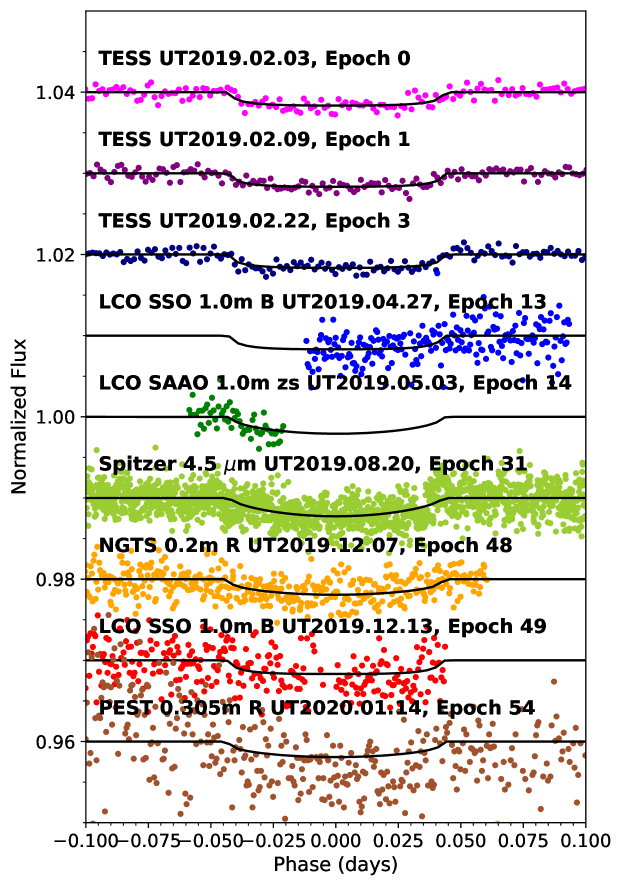
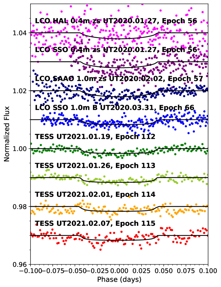
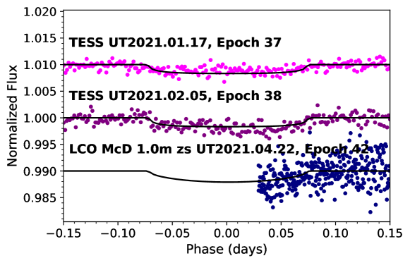
Appendix D RV Models
In this section we show the results if other models that we considered in our RV analysis,
D.1 No Gaussian Process Model for Stellar Activity
Here we present the results of an RV model with no GP applied to account for the stellar activity.
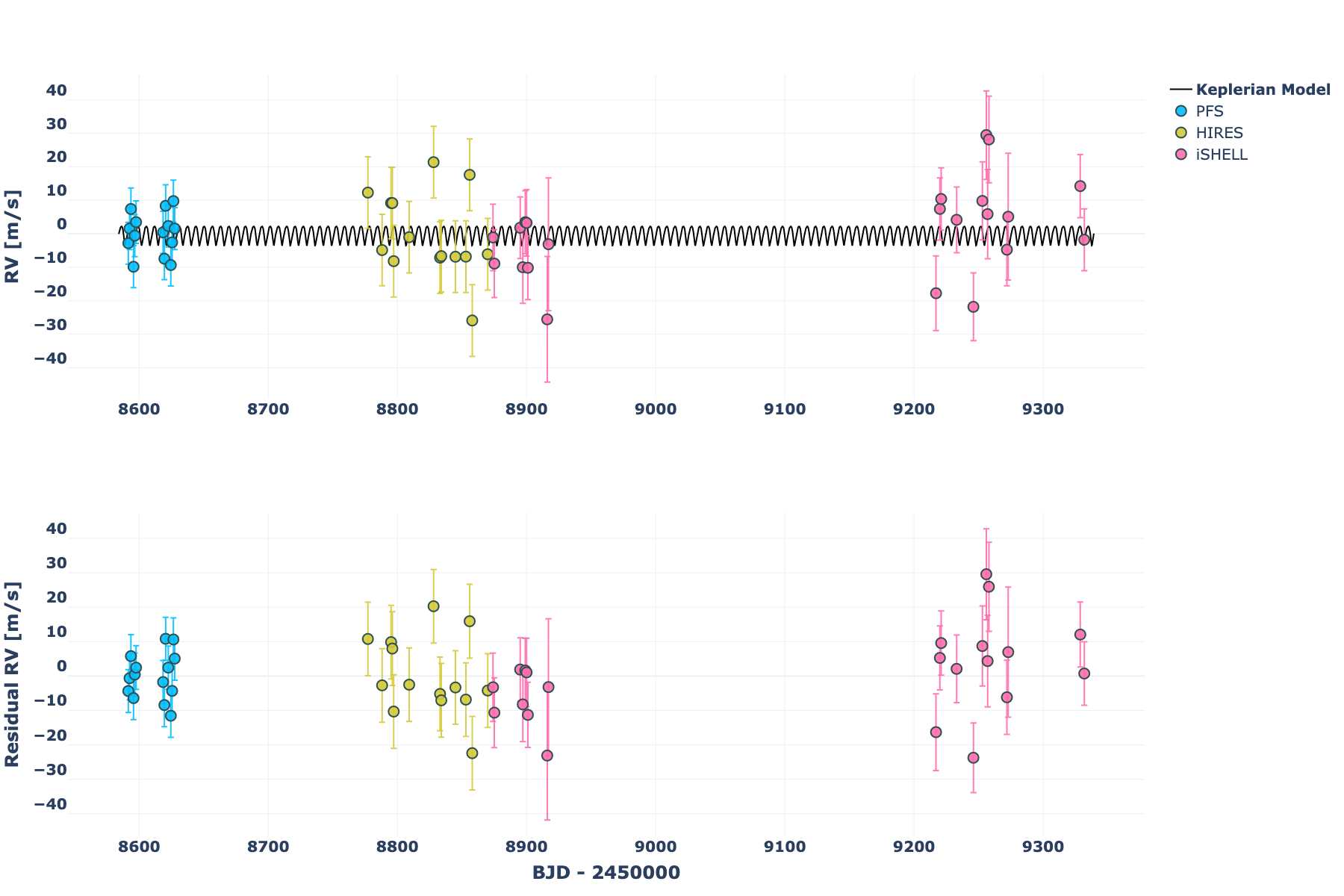
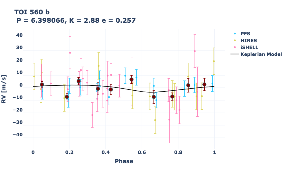
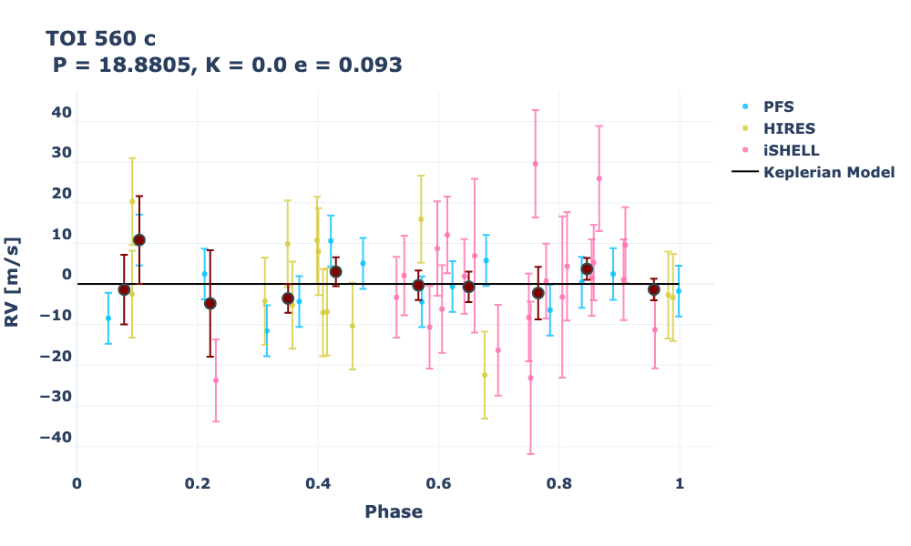
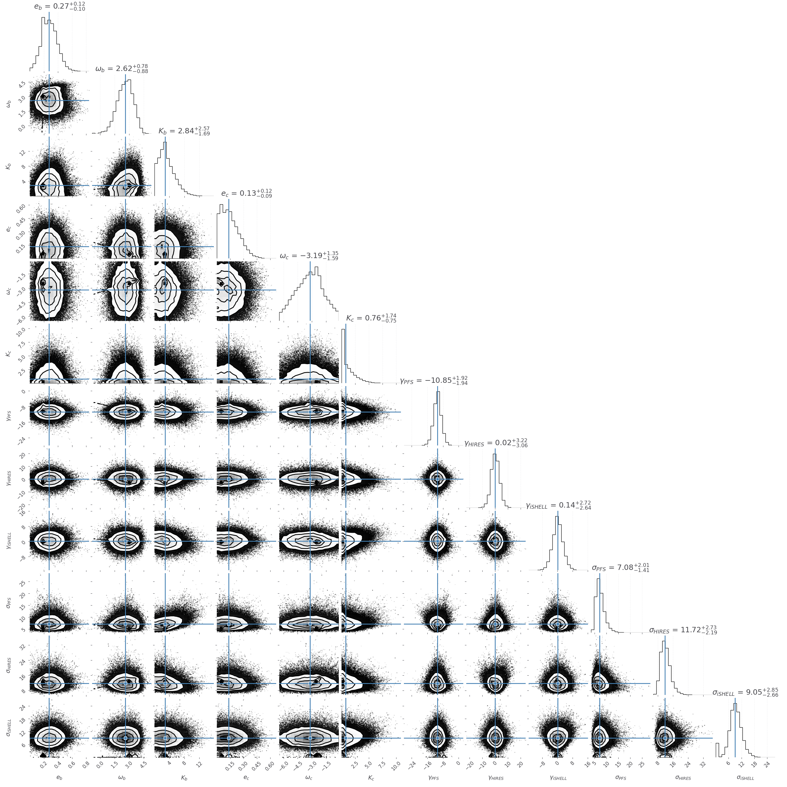
D.2 Joint GP first chromatic kernel J1 model
Here we present the results of an RV model using the joint GP chromatic Kernel J1 model parametrize the stellar activity amplitude through a linear kernel where each amplitude is a free parameter, as in Cale et al. (2021).
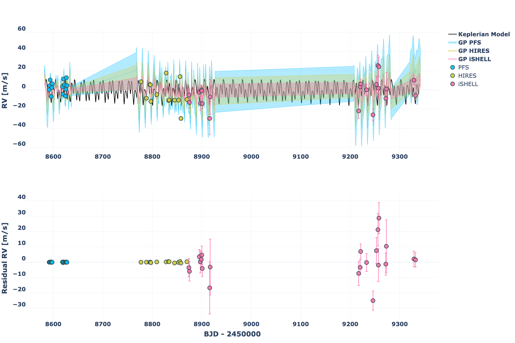
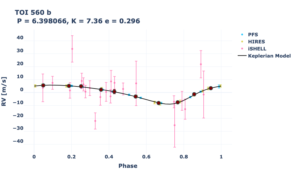
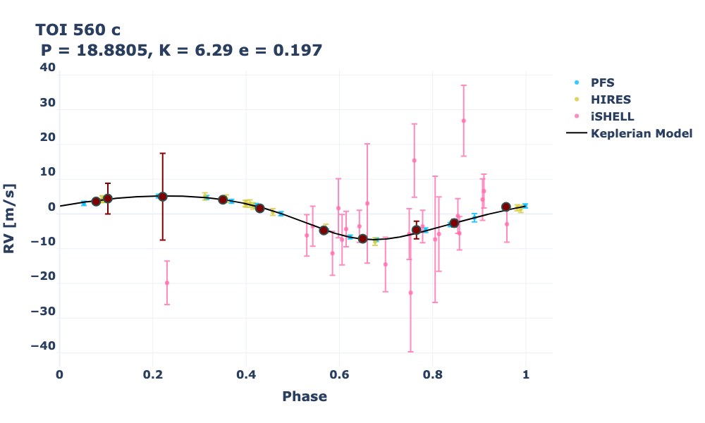
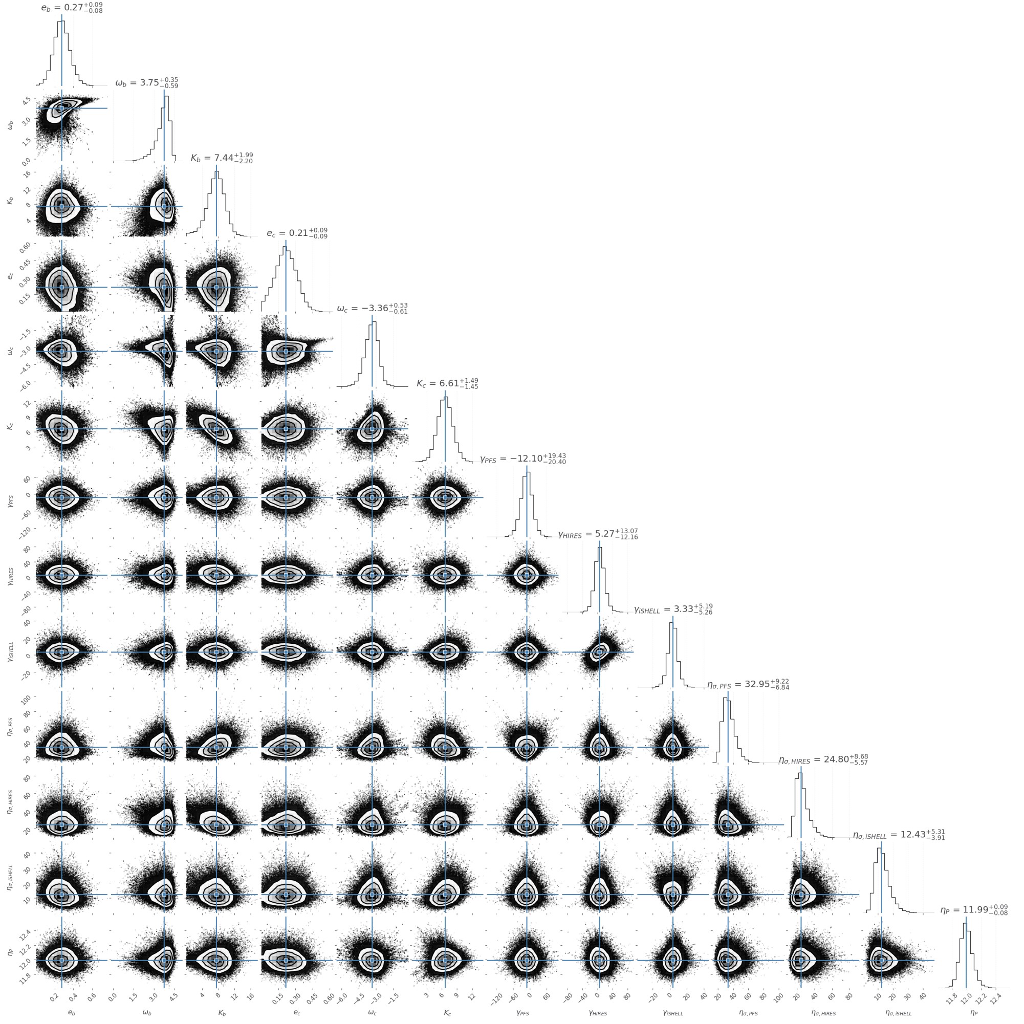
Appendix E Results of our Disjoint Model
This model is using an independent (disjoint) GP to model each RV data set, akin to RadVel (Fulton et al., 2017). Given the lack of overlap between RV data sets, and the relatively sparse RV cadence sampling, this RV model yields similar overfit results to our joint kernel analysis in the previous sub-section.
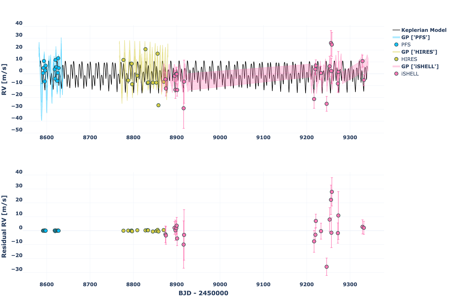
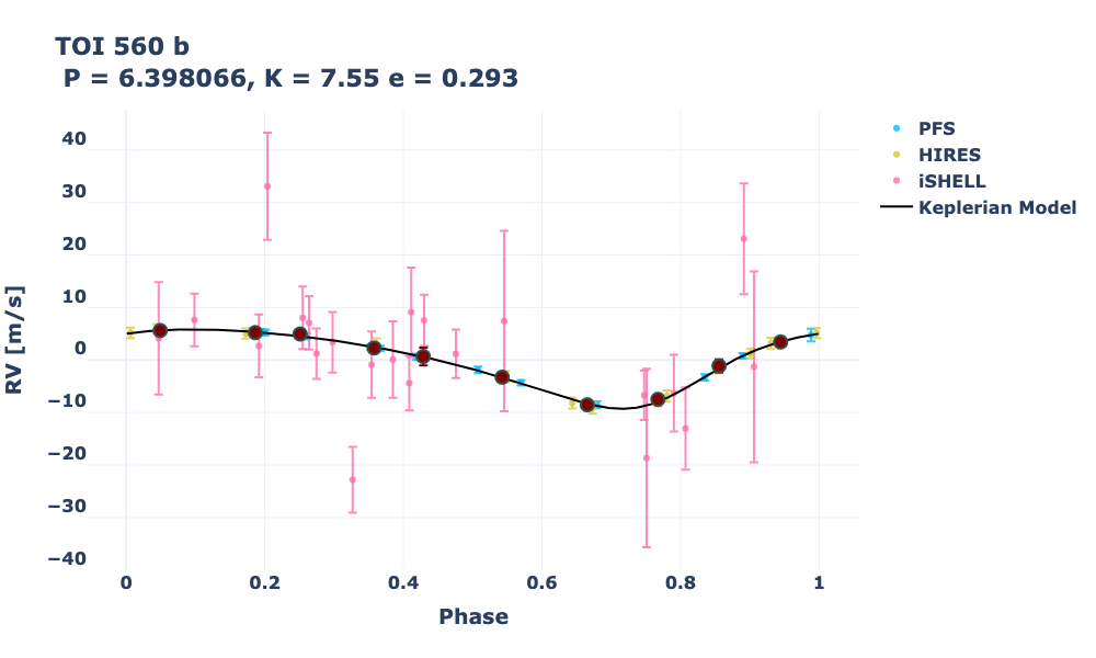
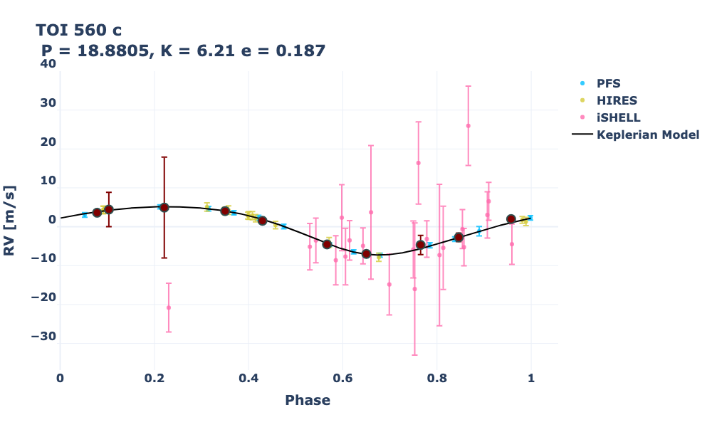
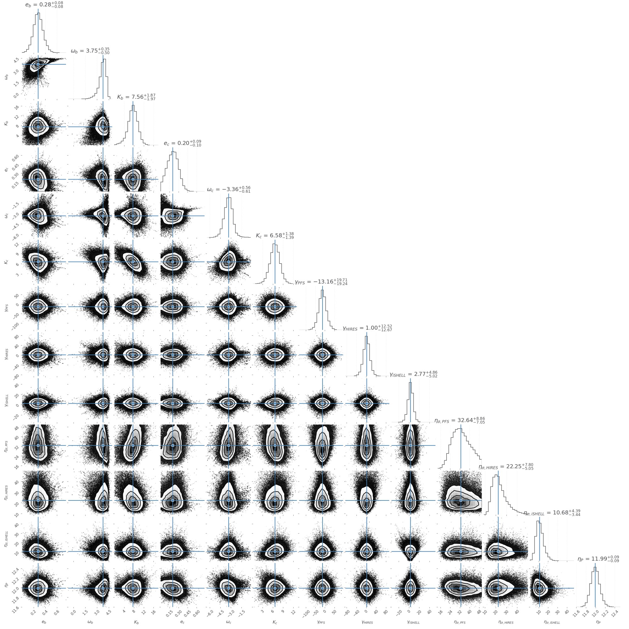
Appendix F Summary of the priors used in the and disjoint kernels
| Parameter [units] | Initial | Priors | MAP | MCMC | MAP | MCMC |
|---|---|---|---|---|---|---|
| Value | Value | Posterior | Value | Posterior | ||
| () | () | () | (Disjoint) | (Disjoint) | ||
| [days] | 6.3980661 | \faLock | – | – | – | – |
| [days] | 2458517.68971 | \faLock | – | – | – | – |
| 0.294 | ; | 0.30 | 0.29 | |||
| ; | 3.87 | 3.81 | ||||
| [m s-1] | 10 | 7.36 | 7.54 | |||
| [days] | 18.8805 | \faLock | – | – | – | – |
| [days] | 2458533.593 | \faLock | – | – | – | – |
| 0.093 | ; | 0.20 | 0.19 | |||
| ; | -3.61 | -3.57 | ||||
| [m s-1] | 10 | 6.29 | 6.21 | |||
| [m s-1] | +1a | ( | 3.73 | 3.15 | ||
| [m s-1] | -13.85 | -14.20 | ||||
| [m s-1] | +1a | 4.34 | 1.19 | |||
| 12.03 | 111.97 | 11.97 | ||||
| 0.44 | \faLock | – | – | – | – | |
| 57.96 | \faLock | – | – | – | – | |
| 9.54 | 8.43 | |||||
| 29.36 | 30.04 | |||||
| 13.63 | 17.34 |
a We want the initial value to be the median of the RVs for that spectrograph; the is used incase the median is already zero, as Nelder-Mead solvers cannot start at zero.
Appendix G Summary of the priors used in the no GP RV analysis
| Parameter [units] | Initial Value () | Priors | MAP Value | MCMC Value |
|---|---|---|---|---|
| [days] | 6.3980661 | \faLock | – | – |
| [days] | 2458517.68971 | \faLock | – | – |
| 0.294 | ; | 0.26 | ||
| , | 2.88 | |||
| [m s-1] | 10 | 2.3 | ||
| [days] | 18.8805 | \faLock | – | – |
| [days] | 2458533.593 | \faLock | – | – |
| 0.093 | ; ; | 0.093 | ||
| , | -3.3 | |||
| [m s-1] | 10 | |||
| [m s-1] | ( | -0.32 | ||
| [m s-1] | -10.9 | |||
| [m s-1] | 0.15 |
a We want the initial value to be the median of the RVs for that spectrograph; the is used incase the median is already zero, as Nelder-Mead solvers cannot start at zero
.
Appendix H Dave Results
Figures 38 and 39 below show the full DAVE vetting results (top table) for the Sectors 8 and 34 light curves respectively. TESS transit data (top row), the binned data (2nd row), and different phased diagnostic plots to look for odd-even effects (third row) secondary, tertiary and “negative” eclipses such as would be produced by false positives (fourth row). Neither analysis identifies statistically significant evidence for a false-positive scenario for TOI 560 b.
Figure 40 shows the photocenter difference images and PSFs for tbe TESS light curves. No significant photocenter motion in transit is observed, helping exclude blended eclipsing binary scenarios.
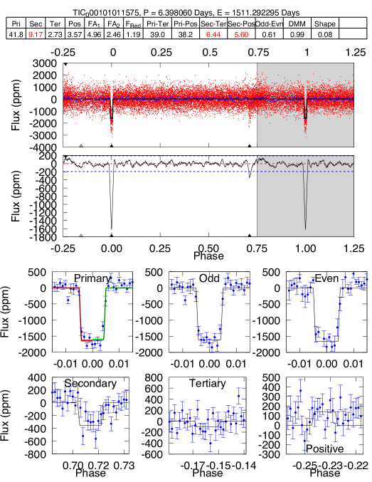
.
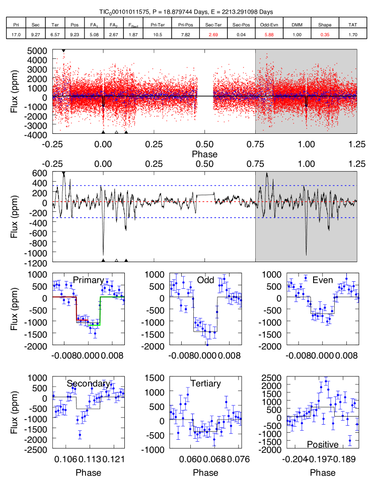
.
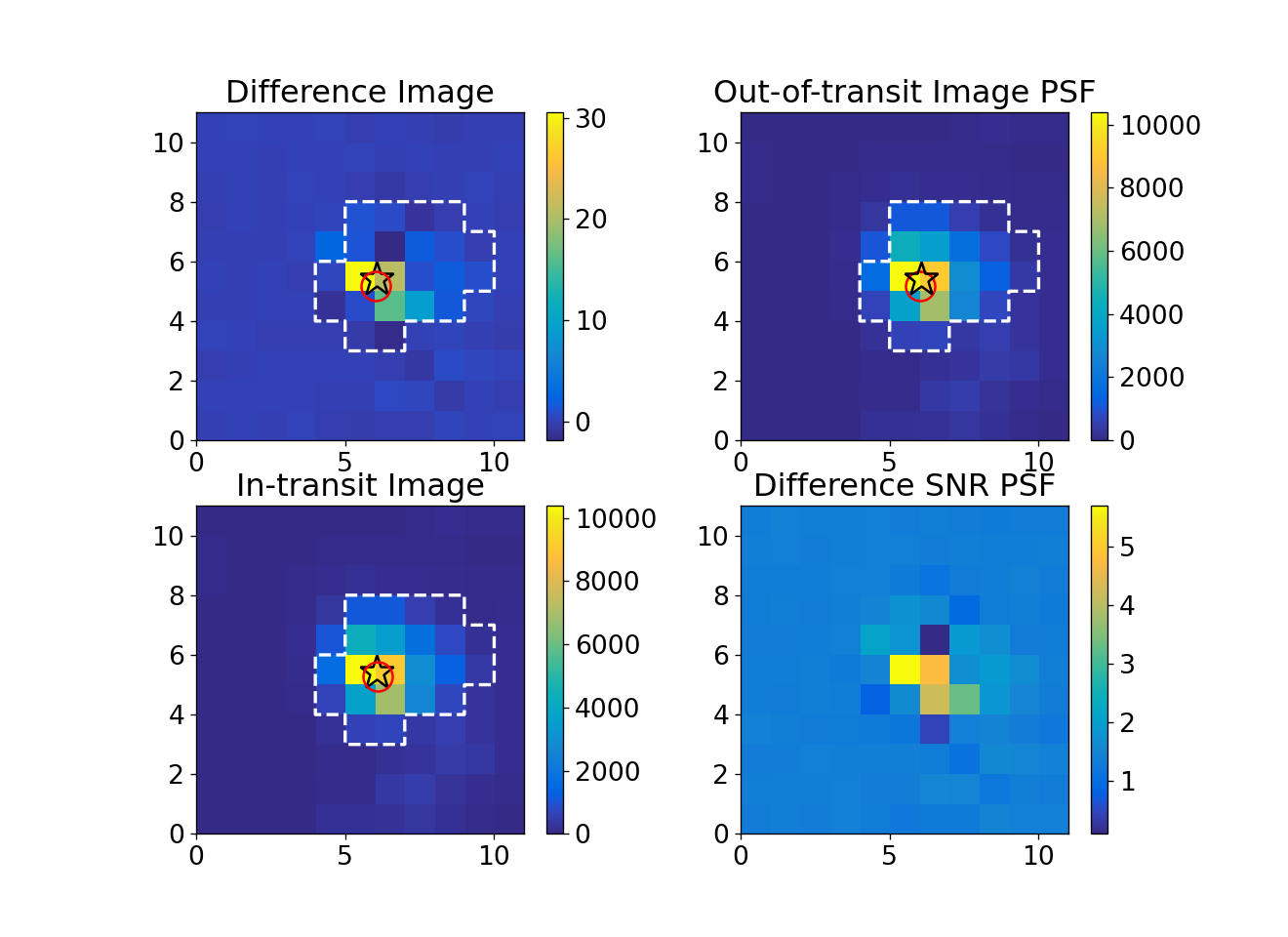
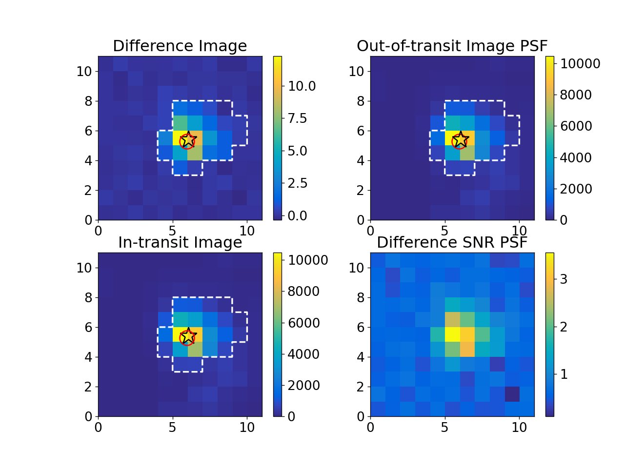
H.1 RVs of our EXOASTv2 analysis
With ExoFASTv2, we carry out an independent RV analysis with no GP to account for stellar activity, as a means of cross-checking our RV analysis with pychell. We recover similar upper-limits and posteriors with both approaches. The phased and unphased RVs from the ExoFASTv2 analysis are shown in Figure 41.
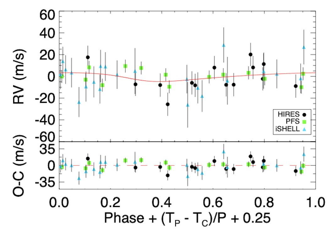
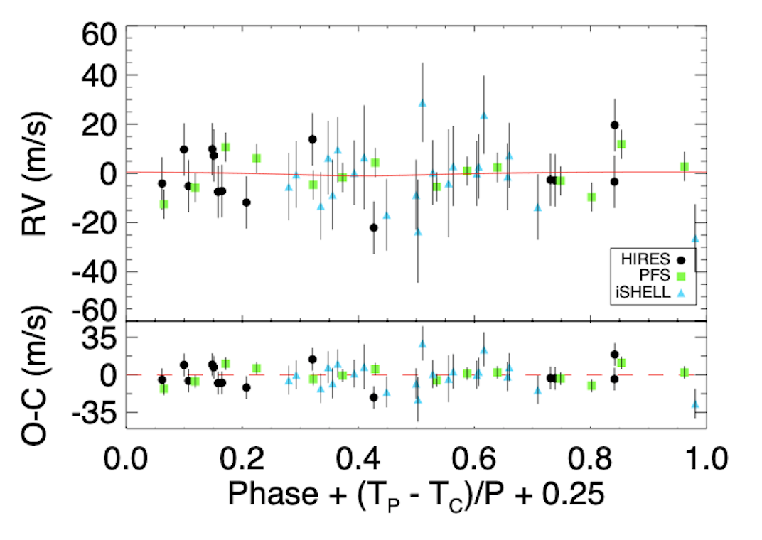
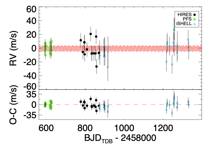
Appendix I Radial Velocities
Table 15 lists the RVs used in our analysis from three different spectrographs, iSHELL, PFS, and HIRES.
| time | mnvel | errvel | tel |
|---|---|---|---|
| 2458874.008515 | -1.466217 | 5.969914 | iSHELL |
| 2458875.0489 | -9.277676 | 6.318843 | iSHELL |
| 2458895.020254 | 1.423469 | 4.620647 | iSHELL |
| 2458897.033761 | -10.358407 | 7.313267 | iSHELL |
| 2458899.005408 | 3.073978 | 5.014754 | iSHELL |
| 2458900.0048987 | 2.879875 | 5.961691 | iSHELL |
| 2458900.988993 | -10.525324 | 5.177452 | iSHELL |
| 2458915.97533 | -25.92508 | 16.986916 | iSHELL |
| 2458916.96779 | -3.498715 | 18.169736 | iSHELL |
| 2459217.043971 | -18.129482 | 7.833479 | iSHELL |
| 2459220.036259 | 7.051904 | 4.807669 | iSHELL |
| 2459221.028598 | 10.012615 | 4.878999 | iSHELL |
| 2459232.98009 | 3.793529 | 5.757477 | iSHELL |
| 2459245.961775 | -22.181634 | 6.264058 | iSHELL |
| 2459252.899543 | 9.439542 | 8.503822 | iSHELL |
| 2459255.971086 | 29.092975 | 10.547535 | iSHELL |
| 2459256.967084 | 5.499865 | 10.704609 | iSHELL |
| 2459257.97079 | 27.775656 | 10.204183 | iSHELL |
| 2459271.925394 | -5.116571 | 7.272103 | iSHELL |
| 2459272.952189 | 4.726328 | 17.173103 | iSHELL |
| 2459328.734044 | 13.861937 | 5.093228 | iSHELL |
| 2459331.828947 | -2.145161 | 4.680086 | iSHELL |
| 2458591.59721 | -13.67 | 0.44 | PFS |
| 2458592.55596 | -9.3 | 0.53 | PFS |
| 2458593.61288 | -3.46 | 0.51 | PFS |
| 2458595.61376 | -20.71 | 0.66 | PFS |
| 2458596.60841 | -11.42 | 0.6 | PFS |
| 2458597.591 | -7.39 | 1.2 | PFS |
| 2458618.52548 | -10.43 | 0.59 | PFS |
| 2458619.53717 | -18.31 | 0.6 | PFS |
| 2458620.50553 | -2.51 | 0.52 | PFS |
| 2458622.55362 | -8.55 | 0.54 | PFS |
| 2458624.50368 | -20.21 | 0.59 | PFS |
| 2458625.51752 | -13.44 | 0.55 | PFS |
| 2458626.50784 | -1.11 | 0.62 | PFS |
| 2458627.5164 | -9.31 | 0.59 | PFS |
| 2458777.117606 | 12.8465553361664 | 0.874164164066315 | HIRES |
| 2458788.120576 | -4.3158532184062 | 0.883318662643433 | HIRES |
| 2458795.078952 | 9.74058435517379 | 0.96750670671463 | HIRES |
| 2458796.044556 | 9.71581891692533 | 0.99626761674881 | HIRES |
| 2458797.109961 | -7.62476348436288 | 0.957593381404877 | HIRES |
| 2458809.083128 | -0.466031437909477 | 0.951945245265961 | HIRES |
| 2458827.972435 | 21.9254428753361 | 0.960972011089324 | HIRES |
| 2458832.988014 | -6.58019230860952 | 1.08839976787567 | HIRES |
| 2458833.948473 | -6.12234576086814 | 1.06621098518372 | HIRES |
| 2458844.911132 | -6.30641359100671 | 1.05241250991821 | HIRES |
| 2458852.955442 | -6.28103672598236 | 0.923207104206085 | HIRES |
| 2458855.901039 | 18.1420626828827 | 1.26564979553223 | HIRES |
| 2458857.895081 | -25.3380374118174 | 1.04208660125732 | HIRES |
| 2458869.88686 | -5.56625046683735 | 1.06461870670319 | HIRES |