Over-the-Air Computation with DFT-spread OFDM for Federated Edge Learning

Abstract

In this study, we propose an over-the-air computation (AirComp) scheme for federated edge learning (FEEL) without channel state information (CSI) at the edge devices or the edge server (ES). The proposed scheme relies on non-coherent communication techniques for achieving distributed training by MV. In this work, the votes, i.e., the signs of the local gradients, from the EDs are represented with the PPM symbols constructed with -spread (DFT-s-OFDM). By taking the delay spread and time-synchronization errors into account, the MV at the ES is obtained with an energy detector. Hence, the proposed scheme does not require CSI at the EDs and ES. We also prove the convergence of the distributed training when the MV is obtained with the proposed scheme under fading channel. Through simulations, we show that the proposed scheme provides a high test accuracy in fading channels while resulting in lower peak-to-mean envelope power ratio (PMEPR) symbols.

I Introduction

FEEL is an implementation of federated learning (FL) over a wireless network to train a model by using the local data at the EDs without uploading them to an ES [1, 2]. Within each iteration of FEEL, a substantial number of parameters (e.g., model parameters or model updates) from each ED needs to be transmitted to the ES for aggregation. Thus, the communication aspect of FEEL is one of the major bottlenecks. One of the promising solutions to this issue is to perform the aggregation by utilizing the signal-superposition property of a wireless multiple access channel [3, 4, 5], i.e., AirComp. However, an AirComp scheme often requires CSI at either the EDs or ES to maintain coherent superposition of the signals from EDs, which can cause a non-negligible overhead and unreliable aggregation in a mobile wireless network. In this study, we address this issue with a new AirComp method.

In the literature, FEEL is investigated with several notable AirComp schemes. In [6], the transmission of the local model parameters at the EDs over OFDM subcarriers are proposed to achieve model parameter aggregation. To reverse the effect of the multipath channel on the transmitted signals, truncated-channel inversion (TCI) is applied, where the symbols on the OFDM subcarriers are multiplied with the inverse of the channel coefficients and the subcarriers that fade are excluded from the transmissions. In [7], one-bit broadband digital aggregation (OBDA), inspired by distributed training by MV [8], is proposed. In this method, the EDs transmit quadrature phase-shift keying (QPSK) symbols over OFDM subcarriers with TCI, where the signs of the elements, i.e., votes, of the local stochastic gradient vectors to form the real and imaginary parts of the QPSK symbols. At the ES, the signs of the real and imaginary components of the superposed symbols on each subcarrier, i.e., the MV, are used to estimate the global gradients. Despite the fact that OBDA is compatible with digital modulations, for AirComp, each ED still requires CSI for TCI. In [9] and [10], the CSI is not available at the EDs, i.e., blind EDs. However, it is assumed that CSI between each ED and ES is available at the ES. To the best of our knowledge, there is no AirComp scheme where CSI is unavailable to both the EDs and the ES for FEEL in the documented literature.

In this study, we propose an AirComp scheme for FEEL without CSI at the EDs and ES. By considering distributed training by MV, we use PPM to encode the votes, where the pulses are synthesized with DFT-s-OFDM[11]. Since the proposed scheme determines the MV with an energy detector applied to the superposed PPM symbols, the CSI is not needed at the EDs and the ES. We also discuss the design with the consideration of the delay spread and the synchronization errors in the time domain. Finally, we prove the convergence of distributed training when the MV is obtained with the proposed scheme under fading channel.

Notation: The complex and real numbers are denoted by $\mathbb{C}$ and $\mathbb{R}$, respectively. ${\mathbb{E}}\left[\cdot\right]$ is the expectation. The sign function is denoted by $\operatorname{sign}(\cdot)$ and results in $1$, $-1$, or $\pm 1$ at random for a positive, a negative, or a zero-valued argument, respectively. We use the notation $(\textbf{a})_{i}^{j}$ as shorthand for denoting a vector $[{a}_{i},{a}_{i+1},\hbox to10.00002pt{.\hss.\hss.},{a}_{j}]^{\rm T}$. The $N$-dimensional all zero vector and $N\times N$ identity matrix are $\textbf{{0}}_{N}$ and $\textbf{{I}}_{N}$, respectively. $\mathbb{I}\left[{\cdot}\right]$ is the indicator function and $\mathbb{P}\left[{\cdot}\right]$ is the probability of its argument.

II System Model

II-A Distributed Training by Majority Vote

Consider a network that consist of $K$ EDs communicating with an ES. Let $\mathcal{D}_{k}$ denote the local data containing labeled data samples at the $k$th ED as $\{({\textrm{{x}}}_{{\ell}},{y}_{{\ell}})\}\in\mathcal{D}_{k}$ for $k=1,\hbox to10.00002pt{.\hss.\hss.},K$, where ${\textrm{{x}}}_{{\ell}}$ and ${y}_{{\ell}}$ are ${\ell}$th data sample and its associated label, respectively. In the case of availability of the local data at the ES (e.g., each ED uploads its data to the ES), the centralized learning problem can be defined as

$${\textbf{w}^{*}}=\arg\min_{\textbf{w}}F(\textbf{w})=\arg\min_{\textbf{w}}\frac{1}{|\mathcal{D}|}\sum_{\forall({\textrm{{x}}},{y})\in\mathcal{D}}f(\textbf{w},{\textrm{{x}}},{y})~{},$$ (1)

where $\mathcal{D}=\mathcal{D}_{1}\cup\mathcal{D}_{2}\cup\cdots\cup\mathcal{D}_{K}$ and $f(\textbf{w},{\textrm{{x}}},{y})$ is the sample loss function that measures the labeling error for $({\textrm{{x}}},{y})$ for the parameters $\textbf{w}=[{w}_{1},\hbox to10.00002pt{.\hss.\hss.},{w}_{q}]^{\rm T}\in\mathbb{R}^{q}$, and $q$ is the number of parameters. In the case of distributed training (e.g., the data is not available at the ES as in FL), one way of solving (1) relies on communicating the gradients between the ES and EDs. To reduce the cost of communicating gradients between the ES and EDs, sign stochastic gradient descend (signSGD) with MV is proposed in [8]. With this method, the updates at the $n$th communication round can be expressed as

$$\textbf{w}^{(n+1)}=\textbf{w}^{(n)}-\eta\textbf{v}^{(n)}~{},$$ (2)

where $\eta$ is the learning rate and $\textbf{v}^{(n)}=[{v}^{(n)}_{1},\hbox to10.00002pt{.\hss.\hss.},{v}^{(n)}_{q}]^{\rm T}$ is the vector that contains the MVs. Assuming that $|\mathcal{D}_{k}|=D$ for $k=1,\hbox to10.00002pt{.\hss.\hss.},K$, the $i$th coordinate of $\textbf{v}^{(n)}$ is calculated as

$${v}^{(n)}_{i}\triangleq\operatorname{sign}\left(\sum_{k=1}^{K}{\operatorname{sign}\left({\tilde{g}}_{k,i}^{(n)}\right)}\right)=\operatorname{sign}\left(\sum_{k=1}^{K}{{\bar{g}}_{k,i}^{(n)}}\right)~{},$$ (3)

where ${\tilde{g}}_{k,i}^{(n)}$ is the $i$th element of the local stochastic gradient vector given by

$$\tilde{\textbf{g}}_{k}^{(n)}=\nabla F_{k}(\textbf{w}^{(n)})=\frac{1}{n_{\rm b}}\sum_{\forall({\textrm{{x}}}_{{\ell}},{y}_{{\ell}})\in\mathcal{\tilde{D}}_{k}}\nabla f(\textbf{w}^{(n)},{\textrm{{x}}}_{{\ell}},{y}_{{\ell}})~{},$$ (4)

where $\mathcal{\tilde{D}}_{k}\subset\mathcal{D}_{k}$ is the selected data batch from the local data samples and $n_{\rm b}=|\mathcal{\tilde{D}}_{k}|$ is the batch size. The corresponding MV-based training procedure can be outlined as follows: The ES first pulls $\bar{\textbf{g}}_{k}^{(n)}=[{\bar{g}}_{k,1}^{(n)},\hbox to10.00002pt{.\hss.\hss.},{\bar{g}}_{k,q}^{(n)}]^{\rm T}$ from all EDs. After calculating (3), $\forall i$, it pushes the MV vector $\textbf{v}^{(n)}$ to the EDs. The EDs then update their parameters as in (2) for the next communication round. Since this method communicates only the signs between EDs and ES, it reduces the cost of communicating the gradients. In this study, we consider the same training procedure for FEEL. However, we use it over a wireless network and develop an AirComp scheme to obtain the MV, inspired by (3), under fading channels.

II-B Signal Model

Consider a wireless network where each ED and the ES are equipped with single antennas. We assume that the EDs’ average signal powers are identical at the ES’s location (i.e., large-scale impacts of the channel are compensated) and managed with an uplink power control mechanism, e.g., through physical random access channel (PRACH) and/or physical uplink control channel (PUCCH) in 3GPP Fifth Generation (5G) New Radio (NR) [12]. We consider the fact the time-synchronization between the EDs may not be perfect and the maximum difference between time of arriving EDs signals at the ES’s location is $T_{\rm sync}$ seconds.

We assume that the EDs access the wireless channel on the same time-frequency resources with $S$ DFT-s-OFDM symbols at the $n$th round. The $m$th transmitted baseband DFT-s-OFDM symbol in discrete time for the $k$th ED can be expressed as

$$\textbf{{t}}_{k,m}^{(n)}=\textbf{{F}}_{N_{\rm IDFT}}^{\rm H}\textbf{{M}}_{\textrm{f}}\textbf{{D}}_{M}\textbf{{d}}_{k,m}^{(n)}~{},$$ (5)

where $\textbf{{F}}_{N_{\rm IDFT}}^{\rm H}\in\mathbb{C}^{N_{\rm IDFT}\times N_{\rm IDFT}}$ is the $N_{\rm IDFT}$-point inverse DFT (IDFT) matrix, $\textbf{{D}}_{M}\in\mathbb{C}^{M\times M}$ is the $M$-point DFT matrix, $\textbf{{M}}_{\textrm{f}}\in\mathbb{R}^{N_{\rm IDFT}\times M}$ is the mapping matrix that maps the output of the DFT precoder to a set of contiguous subcarriers, and $\textbf{{d}}_{k,m}^{(n)}\in\mathbb{C}^{M}$ contains the symbols on $M$ bins. Note that DFT-s-OFDM is a special single-carrier (SC) waveform using circular convolution [11], where the symbol spacing in time is $T_{\rm spacing}=N_{\rm IDFT}T_{\rm sample}/M$ seconds, the pulse shape is Dirichlet sinc [13], and $T_{\rm sample}$ is the sample period.

In this study, we assume the cyclic prefix (CP) duration is larger than the maximum-excess delay denoted by $T_{\rm chn}$ seconds. Hence, assuming the transmissions from the EDs arrive at the ES within the CP duration, the $m$th received baseband signal in discrete-time can be written as

$$\textbf{{r}}_{m}^{(n)}=\sum_{k=1}^{K}\textbf{{H}}_{k}^{(n)}\textbf{{t}}_{k,m}^{(n)}+\textbf{{n}}_{m}^{(n)}~{},$$ (6)

where $\textbf{{H}}_{k}^{(n)}\in\mathbb{C}^{N_{\rm IDFT}\times N_{\rm IDFT}}$ is a circular-convolution matrix based on the channel impulse response (CIR) between the $k$th ED and the ES and $\textbf{{n}}_{m}^{(n)}\sim\mathcal{CN}(\textbf{{0}}_{N_{\rm IDFT}},\sigma_{\rm n}^{2}\textbf{{I}}_{N_{\rm IDFT}})$ is the additive white Gaussian noise (AWGN). At the ES, we calculate the aggregated symbols on the bins as $\tilde{\textbf{{{d}}}}_{m}^{(n)}=\textbf{{D}}_{M}^{\rm H}\textbf{{M}}_{\textrm{f}}^{\rm H}\textbf{{F}}_{N_{\rm IDFT}}\textbf{{r}}_{m}^{(n)}$. Note that we do not use frequency-domain equalization (FDE) since we use DFT-s-OFDM for calculating the MV with a non-coherent detector.

II-C Performance Metrics

II-C1 PMEPR

We define the PMEPR as $\max_{t\in[0,T_{\rm s})}|x(t)|^{2}/{P_{\rm tx}}$, where $x(t)\in\mathbb{C}$ is the baseband OFDM/DFT-s-OFDM symbol in continuous time, $T_{\rm s}$ is the symbol duration, and $P_{\rm tx}={\mathbb{E}_{t}}\left[|x(t)|^{2}\right]=M/N_{\rm IDFT}$ is the mean-envelope power as $\lVert{\textbf{{d}}_{k,m}^{(n)}}\rVert_{2}^{2}$ is equal to $M$ since all bins are actively utilized.

II-C2 Convergence rate

In this study, we define the convergence rate [7, 8] as the rate at which the expected value of average norm of the gradient of $F(\textbf{w})$ diminishes as the number of total communication rounds $N$ and $K$ when the training is done in the presence of the proposed scheme.

III Majority Vote with PPM in Fading Channel

III-A Edge Devices - Transmitter

At the $k$th ED’s transmitter, we encode the signs of the local gradients, i.e., $\{{\bar{g}}_{k,i}^{(n)}\}$, $\forall i,k$, with PPM. We synthesize the pulse in a PPM symbol by activating consecutive $M_{\rm pulse}$ bins of DFT-s-OFDM, which effectively corresponds to a pulse with the duration of $T_{\rm pulse}\approx M_{\rm pulse}T_{\rm spacing}$ seconds by combining $M_{\rm pulse}$ shifted versions of the Dirichlet sinc functions in time. To accommodate the time-synchronization errors and the delay spread, we consider a guard period between the adjacent pulses. Thus, we deactivate the following $M_{\rm gap}$ bins after $M_{\rm pulse}$ active bins, which results in a guard period with the duration of $T_{\rm gap}\approx M_{\rm gap}T_{\rm spacing}$ seconds, where $T_{\rm gap}\geq T_{\rm chn}+T_{\rm sync}$ must hold true. As a result, the maximum number of votes that can be carried for each DFT-s-OFDM symbol can be calculated as $M_{\rm vote}=\left\lfloor\frac{M}{2(M_{\rm pulse}+M_{\rm gap})}\right\rfloor$, where $M_{\rm gap}\geq\lceil(T_{\rm chn}+T_{\rm sync})/T_{\rm spacing}\rceil$.

In this study, we consider a generalized mapping rule that maps the signs of the local gradients to the positions of the pulses within a DFT-s-OFDM symbol and $S$ DFT-s-OFDM symbols. To this end, let ${f}$ be a function that maps $i\in\{1,2,\hbox to10.00002pt{.\hss.\hss.},q\}$ to the distinct pairs $(m^{+},l^{+})$ and $(m^{-},l^{-})$ that indicate the pulse positions for $m^{+},m^{-}\in\{0,1,\hbox to10.00002pt{.\hss.\hss.},S-1\}$ and $l^{+},l^{-}\in\{0,1,\hbox to10.00002pt{.\hss.\hss.},2M_{\rm vote}-1\}$. For all $i$, we then determine the following bins of DFT-s-OFDM symbols as

$$(\textbf{{d}}_{k,{m^{+}}}^{(n)})_{l^{+}(M_{\rm pulse}+M_{\rm gap})}^{l^{+}(M_{\rm pulse}+M_{\rm gap})+M_{\rm pulse}-1}=\textbf{p}s_{k,i}^{(n)}\mathbb{I}\left[{{\bar{g}}_{k,i}^{(n)}=1}\right]~{},$$

and

$$(\textbf{{d}}_{k,{m^{-}}}^{(n)})_{l^{-}(M_{\rm pulse}+M_{\rm gap})}^{l^{-}(M_{\rm pulse}+M_{\rm gap})+M_{\rm pulse}-1}=\textbf{p}s_{k,i}^{(n)}\mathbb{I}\left[{{\bar{g}}_{k,i}^{(n)}=-1}\right]~{},$$

where $\textbf{p}\in\mathbb{C}^{M_{\rm pulse}}$ contains the weights of the Dirichlet sinc functions to generate the pulse, and $s_{k,i}^{(n)}$ is a random symbol on the unit-circle. Therefore, the proposed scheme defines two pulse positions over two different time resources for one vote. If $m^{+}=m^{-}$ and $l^{+}=l^{-}+1$ for all $i$, the adjacent time resources of $m^{+}$th DFT-s-OFDM symbol are used for voting. The MV calculation with proposed scheme under this specific mapping is referred to as -based (PPM-MV) in this study.

III-A1 Pulse Shape

We choose p as $\sqrt{E_{\rm s}}\times[1,-1,1,-1,\cdots]^{\rm T}$ since this sequence yields a rectangular-like pulse shape in the time domain for DFT-s-OFDM, as illustrated in Section IV, where $E_{\rm s}=2(M_{\rm pulse}+M_{\rm gap})/M_{\rm pulse}$ is an energy normalization factor. It is worth noting that the proposed framework allows one to design p for various pulse shapes, which can be considered for further optimization of the proposed scheme.

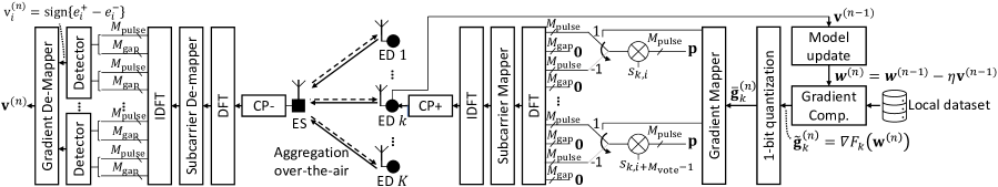
Figure 1: Transmitter and receiver diagrams for PPM-MV with DFT-s-OFDM for FEEL.

III-B Edge Server - Receiver

At the ES, we first calculate the pairs $(m^{+},l^{+})$ and $(m^{-},l^{-})$ based on ${f}$ for a given $i$. We then obtain the MV for the $i$th gradient with an energy detector as

$${v}^{(n)}_{i}=\operatorname{sign}\left({\Delta}^{(n)}_{i}\right)~{},$$ (7)

where ${\Delta}^{(n)}_{i}\triangleq{e_{i}^{+}-e_{i}^{-}}$ for

$$e_{i}^{+}\triangleq\lVert(\tilde{\textbf{{{d}}}}_{m^{+}}^{(n)})_{l^{+}(M_{\rm pulse}+M_{\rm gap})}^{l^{+}(M_{\rm pulse}+M_{\rm gap})+M_{\rm pulse}+M_{\rm gap}-1}\rVert_{2}^{2}~{},$$ (8)

and

$$e_{i}^{-}\triangleq\lVert(\tilde{\textbf{{{d}}}}_{m^{-}}^{(n)})_{l^{-}(M_{\rm pulse}+M_{\rm gap})}^{l^{-}(M_{\rm pulse}+M_{\rm gap})+M_{\rm pulse}+M_{\rm gap}-1}\rVert_{2}^{2}~{}.$$ (9)

Since the multipath channel disperses the pulses in the time domain and the synchronization error changes the position of the pulse in time, we consider $M_{\rm pulse}+M_{\rm gap}$ bins for the energy calculations in (8) and (9).

In Figure 1, the transmitter and the receiver block diagrams are provided based on the aforementioned discussions.

III-C Why Does It Work without CSI at the EDs and ES?

Let $K^{+}_{i}$ and $K^{-}_{i}=K-K^{+}_{i}$ be the numbers of EDs that contribute a vote towards $1$ and $-1$ for the $i$th gradient, respectively. It is trivial to show that ${e_{i}^{+}}$ and ${e_{i}^{-}}$ are exponential random variables, where their means are approximately $\mu^{+}_{i}\triangleq{\mathbb{E}}\left[e_{i}^{+}\right]\approx M_{\rm pulse}E_{\rm s}K^{+}_{i}+(M_{\rm pulse}+M_{\rm gap})\sigma_{\rm n}^{2}$ and $\mu^{-}_{i}\triangleq{\mathbb{E}}\left[e_{i}^{-}\right]\approx M_{\rm pulse}E_{\rm s}K^{-}_{i}+(M_{\rm pulse}+M_{\rm gap})\sigma_{\rm n}^{2}$. Since $\mu^{+}_{i}$ and $\mu^{-}_{i}$ are linear functions of $K^{+}_{i}$ and $K^{-}_{i}$, respectively, the proposed scheme obtains the correct MV probabilistically as the PPM symbols may not coherently add up and their amplitudes may not be aligned in fading channel. Therefore, the MV calculated in (7) is different from the original MV given in (3). Hence, to provide a convincing answer to the question if the proposed scheme maintains the convergence of the original MV in [8], we need to show the convergence for a non-convex loss function $F(\textbf{w})$. To this end, we consider several standard assumptions made in the literature [8, 7]:

Assumption 1 (Bounded loss function).

$F(\textbf{w})\geq F^{*}$, $\forall\textbf{w}$.

Assumption 2 (Smooth).

Let g be the gradient of $F(\textbf{w})$ evaluated at w. For all w and $\textbf{w}^{\prime}$, the expression given by

$$\left|F(\textbf{w}^{\prime})-(F(\textbf{w})+{\textbf{{g}}}^{\rm T}(\textbf{w}^{\prime}-\textbf{w}))\right|\leq\frac{1}{2}\sum_{i=1}^{q}L_{i}({w}_{i}^{\prime}-{w}_{i})^{2}~{},$$

holds for a non-negative constant vector $\textbf{L}=[L_{1},\hbox to10.00002pt{.\hss.\hss.},L_{q}]^{\rm T}$.

Assumption 3 (Variance bound).

The stochastic gradient estimates $\{\tilde{\textbf{g}}_{k}=[{\tilde{g}}_{k,1},\hbox to10.00002pt{.\hss.\hss.},{\tilde{g}}_{k,q}]^{\rm T}=\nabla F_{k}(\textbf{w}^{(n)})\}$, $\forall k$, are independent and unbiased estimates of ${\textbf{{g}}}=[{g_{1}},\hbox to10.00002pt{.\hss.\hss.},{g_{q}}]^{\rm T}=\nabla F(\textbf{w})$ with a coordinate bounded variance, i.e.,

$${\mathbb{E}}\left[\tilde{\textbf{g}}_{k}\right] ={\textbf{{g}}},~{}\forall k,$$ (10)

$${\mathbb{E}}\left[({\tilde{g}}_{k,i}-{g_{i}})^{2}\right] \leq\sigma_{i}^{2}/n_{\rm b},~{}\forall k,i,$$ (11)

where ${\bm{\sigma}}=[\sigma_{1},\hbox to10.00002pt{.\hss.\hss.},\sigma_{q}]^{\rm T}$ is a non-negative constant vector.

Assumption 4 (Unimodal, symmetric gradient noise).

For any given w, the elements of the vector $\tilde{\textbf{g}}_{k}$, $\forall k$, has a unimodal distribution that is also symmetric around its mean.

Theorem 1.

For $n_{\rm b}=N/\gamma$ and $\eta=1/\sqrt{\lVert\textbf{L}\rVert_{1}n_{\rm b}}$, the convergence rate of the distributed training by the MV based on PPM in fading channel is

$${\mathbb{E}}\left[\frac{1}{N}\sum_{n=0}^{N-1}\lVert{\textbf{{g}}}^{(n)}\rVert_{1}\right]\leq\frac{1}{\sqrt{N}} \bigg{(}a\sqrt{\lVert\textbf{L}\rVert_{1}}\left(F(\textbf{w}^{(0)})-F^{*}+\frac{\gamma}{2}\right)$$

$$~{}~{}+\frac{2\sqrt{2\gamma}}{3}\lVert{\bm{\sigma}}\rVert_{1}\bigg{)}~{},$$ (12)

where $a=(1+\frac{2}{\xi K})\frac{1}{\sqrt{\gamma}}$ for $\xi\triangleq\frac{M_{\rm pulse}E_{\rm s}}{(M_{\rm pulse}+M_{\rm gap})\sigma_{\rm n}^{2}}$.

Proof:

Let ${\textbf{{g}}}^{(n)}$ be the gradient of $F(\textbf{w}^{(n)})$ (i.e., the true gradient ). By using Assumption 2 and using (7), we can write

$$F(\textbf{w}^{(n+1)}) -F(\textbf{w}^{(n)})\leq-\eta{{\textbf{{g}}}^{(n)}}^{\rm T}\textbf{v}^{(n)}+\frac{\eta^{2}}{2}\lVert\textbf{L}\rVert_{1}$$

$$= -\eta\lVert{\textbf{{g}}}^{(n)}\rVert_{1}+\frac{\eta^{2}}{2}\lVert\textbf{L}\rVert_{1}$$

$$+2\eta\sum_{i=1}^{q}|{{g}}^{(n)}_{i}|\mathbb{I}\left[{\operatorname{sign}\left({\Delta}^{(n)}_{i}\right)\neq\operatorname{sign}\left({{g}}^{(n)}_{i}\right)}\right]~{}.$$

Thus,

$${\mathbb{E}}\left[F(\textbf{w}^{(n+1)})-F(\textbf{w}^{(n)})|\textbf{w}^{(n)}\right]\leq-\eta\lVert{\textbf{{g}}}^{(n)}\rVert_{1}+\frac{\eta^{2}}{2}\lVert\textbf{L}\rVert_{1}$$

$$~{}~{}~{}~{}~{}~{}~{}~{}~{}~{}~{}~{}~{}~{}+\underbrace{2\eta\sum_{i=1}^{q}|{{g}}^{(n)}_{i}|\underbrace{\mathbb{P}\left[{\operatorname{sign}\left({\Delta}^{(n)}_{i}\right)\neq\operatorname{sign}\left({{g}}^{(n)}_{i}\right)}\right]}_{\triangleq P^{\rm err}_{i}}}_{\text{Stochasticity-induced error}}~{}.$$

A bound on the stochasticity-induced error can be obtained as follows: Assume that $\operatorname{sign}\left({{g}}^{(n)}_{i}\right)=1$. Let $Z$ be a random variable for counting the number of EDs with the correct decision, i.e., $\operatorname{sign}\left({{g}}^{(n)}_{i}\right)=1$. The random variable $Z$ can then be model as the sum of $K$ independent Bernoulli trials, i.e., a binomial variable with the success and failure probabilities given by

$$p_{i}\triangleq\mathbb{P}\left[{\operatorname{sign}\left({\tilde{g}}_{k,i}^{(n)}\right)=\operatorname{sign}\left({{g}}^{(n)}_{i}\right)}\right]~{},$$

$$q_{i}\triangleq\mathbb{P}\left[{\operatorname{sign}\left({\tilde{g}}_{k,i}^{(n)}\right)\neq\operatorname{sign}\left({{g}}^{(n)}_{i}\right)}\right]~{},$$

respectively, for all $k$. This implies that

$$P^{\rm err}_{i}=\sum_{K^{+}_{i}=0}^{K}\mathbb{P}\left[{{\operatorname{sign}\left({\Delta}^{(n)}_{i}\right)\neq 1}|Z=K^{+}_{i}}\right]\mathbb{P}\left[{Z=K^{+}_{i}}\right]~{},$$

where $\mathbb{P}\left[{Z=K^{+}_{i}}\right]=\binom{K}{K^{+}_{i}}p_{i}^{K^{+}_{i}}q_{i}^{K-K^{+}_{i}}$. To calculate $\mathbb{P}\left[{{\operatorname{sign}\left({\Delta}^{(n)}_{i}\right)\neq 1}|Z=K^{+}_{i}}\right]$, we use the distribution of ${\Delta}^{(n)}_{i}$, which can be obtained by using the properties of exponential random variables as

$$f({\Delta}^{(n)}_{i})=\begin{cases}\frac{{\rm e}^{-\frac{{\Delta}^{(n)}_{i}}{\mu^{-}_{i}}}}{\mu^{+}_{i}+\mu^{-}_{i}},&{\Delta}^{(n)}_{i}\leq 0\\ \frac{{\rm e}^{-\frac{{\Delta}^{(n)}_{i}}{\mu^{+}_{i}}}}{\mu^{+}_{i}+\mu^{-}_{i}},&{\Delta}^{(n)}_{i}>0\end{cases}~{}.$$ (13)

Thus, by integrating (13) with respect to ${\Delta}^{(n)}_{i}$,

$$\mathbb{P}\left[{{\operatorname{sign}\left({\Delta}^{(n)}_{i}\right)\neq 1}|Z=K^{+}_{i}}\right] =\frac{\mu^{-}_{i}}{\mu^{+}_{i}+\mu^{-}_{i}}=\frac{(K-K^{+}_{i})+1/\xi}{K+2/\xi}.$$ (14)

Hence, by using (14) and the properties of binomial coefficients

$$P^{\rm err}_{i} =\sum_{K^{+}_{i}=0}^{K}\frac{(K-K^{+}_{i})+1/\xi}{1+2/\xi}\binom{K}{K^{+}_{i}}p_{i}^{K^{+}_{i}}q_{i}^{K-K^{+}_{i}}=\frac{\frac{1}{\xi K}+q_{i}}{1+\frac{2}{K\xi}}~{}.$$

Under Assumption 2 and Assumption 3, by using the derivations in [8], $q_{i}\leq\frac{\sqrt{2}\sigma_{i}}{3|{{g}}^{(n)}_{i}|\sqrt{n_{\rm b}}}$ holds true. Hence, an upper bound on the stochasticity-induced error can be obtained as

$$\sum_{i=1}^{q}|{{g}}^{(n)}_{i}|P^{\rm err}_{i}\leq\frac{\frac{1}{\xi K}}{1+\frac{2}{K\xi}}\lVert{\textbf{{g}}}^{(n)}\rVert_{1}+\frac{1}{\sqrt{n_{\rm b}}}\frac{\sqrt{2}/3}{1+\frac{2}{K\xi}}\lVert{\bm{\sigma}}\rVert_{1}~{}.$$

Based on Assumption 1, we can show that

$$F(\textbf{w}^{(0)})-F^{*}\geq F(\textbf{w}^{(0)})-{\mathbb{E}}\left[F(\textbf{w}^{(N)})\right]$$

$$={\mathbb{E}}\left[\sum_{n=0}^{N-1}F(\textbf{w}^{(n)})-F(\textbf{w}^{(n+1)})\right]$$

$$\geq{\mathbb{E}}\left[\sum_{n=0}^{N-1}\frac{\eta}{1+\frac{2}{K\xi}}\lVert{\textbf{{g}}}^{(n)}\rVert_{1}-\frac{\eta^{2}}{2}\lVert\textbf{L}\rVert_{1}-\frac{\eta}{\sqrt{n_{\rm b}}}\frac{2\sqrt{2}/3}{1+\frac{2}{K\xi}}\lVert{\bm{\sigma}}\rVert_{1}\right]~{}.$$ (15)

By rearranging the terms in (15) and using the expressions for $n_{\rm b}$ and $\eta$, (12) is reached. ∎

Theorem 1 shows that when $\xi$ and $K$ are large, the convergence with the proposed scheme in fading channel is similar to the one with signSGD in an ideal channel [8, Theorem 1].

III-D Implementation Details, Trade-offs, and Comparisons

The main difference of the proposed scheme as compared to the approaches in [6] and [7] is that it does not need TCI at the EDs and prevents the loss of the gradients due to the truncation. As opposed to the methods in [9] and [10], it also does not require CSI at the ES or multiple antennas. Therefore, the proposed scheme offers practical distributed learning in mobile networks. The second major difference of the proposed scheme is that it leads to an interesting trade-off between PMEPR and resource utilization as shown in Section IV. For a given $M_{\rm gap}$, as $M_{\rm pulse}$ increases, the pulse energy distributes more evenly in time and the amplitude decreases as less votes are carried. This results in a decreasing PMEPR, but more resource consumption. The shortcoming of the proposed scheme is that it consumes a larger number of DFT-s-OFDM symbols as compared to OBDA. Although this appears to be a limitation, we emphasize that the proposed method eliminates the non-negligible channel estimation overhead and is immune to the time-variations of the channel and time synchronization error. Finally, we choose $s_{k,i}^{(n)}$ as random QPSK in this study since this is implementation-friendly and randomizes ${e_{i}^{+}}$ and ${e_{i}^{-}}$ in a static channel, which is needed for obtaining the correct MV probabilistically, as discussed in Section III-C.

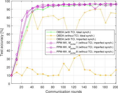
(a) SNR is $0$ dB ($D=400$, $K=50$).

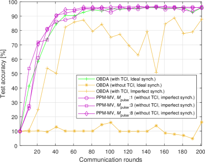
(b) SNR is $20$ dB ($D=400$, $K=50$).

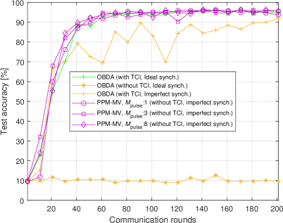
(c) SNR is $0$ dB ($D=2000$, $K=10$).

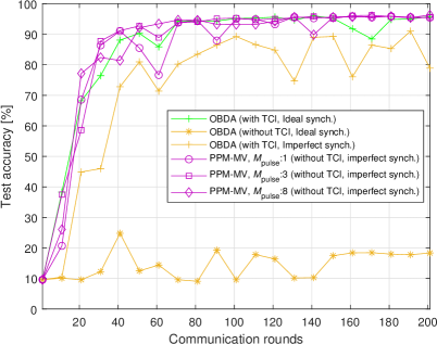
(d) SNR is $20$ dB ($D=2000$, $K=10$).

Figure 2: Test accuracy results in fading channel (ITU EPA). The FEEL with the PPM-MV works without the CSI at the EDs and ES ($n_{\rm b}=64$).

IV Numerical Results

We consider a handwritten-digit recognition learning task over a FEEL system, in which we compare the proposed scheme with OBDA [7]. The learning task uses the MNIST database that contains labeled handwritten-digit images of size $28\times 28$, from 0 to 9. $20000$ training images are randomly partitioned into equal shares for $K\in\{10,50\}$ EDs. We consider a convolutional neural network (CNN) for the model. It consists of one $5\times 5$ and two $3\times 3$ convolutional layers, each consisting of $20$ filters, and the subsequent layers to each are a batch normalization and rectified-linear unit (ReLU) activation layer. Following the final ReLU layer, a fully-connected layer of 10 units corresponding to the 0 to 9 digits and a softmax layer are utilized. The learning rate is set to $0.01$ and $n_{\rm b}=64$. For the test accuracy calculations, we use $10000$ test images given in the database. Our model contains $q=123090$ learnable parameters, which corresponds to $S=52$ OFDM symbols for OBDA with $M=1200$ subcarriers. The OFDM symbol duration $T_{\rm s}$ and the threshold for TCI are set to $66.67~{}\mu$s and $0.2$, respectively. To test FEEL, two different uplink signal-to-noise ratios (i.e., $1/\sigma_{\rm n}^{2}$) of $0$ dB and $20$ dB are considered. ITU Extended Pedestrian A (EPA) with no mobility is considered for the fading channel, and the channels between the EDs and ES are regenerated to capture the long-term channel variations. The root-mean-square (RMS) delay spread of the EPA channel is $T_{\rm rms}=43.1$ ns. As a rule of thumb, we assume that the maximum-excess delay is $T_{\rm chn}\triangleq 4T_{\rm rms}=172.5$ ns. We set the sample rate to $30.72$ Msps and $N_{\rm IDFT}=2048$. Unless otherwise stated, we assume that the maximum synchronization error among the EDs is $T_{\rm sync}=55.6$ ns (i.e., the reciprocal of the signal bandwidth and approximately 2 samples within the CP window). We set $M_{\rm gap}$ to $7$ to ensure that $M_{\rm gap}\geq\lceil(T_{\rm chn}+T_{\rm sync})/T_{\rm spacing}\rceil$ for $T_{\rm spacing}=55.6$ ns. The number of DFT-s-OFDM symbols for $M_{\rm pulse}=1$, $M_{\rm pulse}=3$, $M_{\rm pulse}=8$, and $M_{\rm pulse}=13$ can be then calculated as $1642$, $2052$, $3078$, and $4108$, respectively. The simulations are performed in MATLAB.

The test accuracy results are provided in Figure 2. The OBDA provides high test accuracy in the case of ideal synchronization when TCI presents. This is expected because the MV calculation requires a coherent superposition of the QPSK symbols. However, it completely fails in the absence of TCI. It is also very sensitive to time synchronization errors. On the other hand, PPM-MV results in high test accuracy without TCI or CSI at the ES as it exploits non-coherent techniques for the MV computation and immune against time synchronization errors.

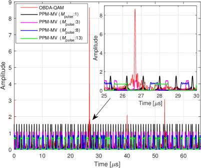
Figure 3: Temporal characteristics.

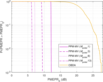
Figure 4: PMEPR distributions.

Figure 3 details the temporal characteristics of OBDA and PPM-MV. We see that the signal can be very peaky with OBDA when all the QPSK symbols are similar to each other. For PPM-MV, this is not an issue as the votes are represented as separated pulses in time. Figure 4 shows the PMEPR for both OBDA and PPM-MV. We show the trade-off that $M_{\rm pulse}$ presents. For OBDA, the PMEPR can be exceptionally high. In contrast, PPM-MV mitigates the PMEPR aggressively, which is an important for factor for radios equipped with non-linear power amplifiers. The trade-off displayed is that as $M_{\rm pulse}$ rises, the PMEPR curve diminishes, but, as demonstrated in Figure 3, more resources in time are consumed.

V Concluding Remarks

Equalization methods used in traditional communications cannot be trivially used with the state-of-the-art AirComp schemes due to the superposition in the wireless channel. This issue causes a major challenge for practical AirComp. To address this problem, in this study, we propose an AirComp method that relies on non-coherent detection and PPM symbols. We show how to design the PPM symbols with DFT-s-OFDM by taking time-synchronization errors into account. The main benefits of the proposed scheme as compared to the state-of-the-art solutions are that it eliminates CSI at the EDs and ES and provides a high test accuracy even when time synchronization is imperfect. Therefore, it offers a promising solution for enabling distributed learning over wireless networks. Also, it reduces the PMEPR as compared to OBDA, where the improvement on PMEPR can be adjusted at the expense of consuming more resources in the time domain.

References

• [1] T. Gafni, N. Shlezinger, K. Cohen, Y. C. Eldar, and H. V. Poor, “Federated learning: A signal processing perspective,” 2021. [Online]. Available: arXiv:2103.17150
• [2] M. Chen, D. Gündüz, K. Huang, W. Saad, M. Bennis, A. V. Feljan, and H. Vincent Poor, “Distributed learning in wireless networks: Recent progress and future challenges,” IEEE J. Sel. Areas Commun., pp. 1–26, 2021.
• [3] M. Goldenbaum, H. Boche, and S. Stańczak, “Harnessing interference for analog function computation in wireless sensor networks,” IEEE Trans. Signal Process., vol. 61, no. 20, pp. 4893–4906, Oct. 2013.
• [4] W. Liu, X. Zang, Y. Li, and B. Vucetic, “Over-the-air computation systems: Optimization, analysis and scaling laws,” IEEE Trans. Wireless Commun., vol. 19, no. 8, pp. 5488–5502, Aug. 2020.
• [5] B. Nazer and M. Gastpar, “Computation over multiple-access channels,” IEEE Trans. Inf. Theory, vol. 53, no. 10, pp. 3498–3516, Oct. 2007.
• [6] G. Zhu, Y. Wang, and K. Huang, “Broadband analog aggregation for low-latency federated edge learning,” IEEE Trans. Wireless Commun., vol. 19, no. 1, pp. 491–506, Jan. 2020.
• [7] G. Zhu, Y. Du, D. Gündüz, and K. Huang, “One-bit over-the-air aggregation for communication-efficient federated edge learning: Design and convergence analysis,” IEEE Trans. Wireless Commun., vol. 20, no. 3, pp. 2120–2135, Nov. 2021.
• [8] J. Bernstein, Y.-X. Wang, K. Azizzadenesheli, and A. Anandkumar, “signSGD: Compressed optimisation for non-convex problems,” in Proc. in International Conference on Machine Learning, vol. 80.   Proceedings of Machine Learning Research, 10–15 Jul 2018, pp. 560–569.
• [9] K. Yang, T. Jiang, Y. Shi, and Z. Ding, “Federated learning via over-the-air computation,” IEEE Trans. Wireless Commun., vol. 19, no. 3, pp. 2022–2035, 2020.
• [10] M. M. Amiria, T. M. Duman, D. Gündüz, S. R. Kulkarni, and H. Vincent Poor, “Collaborative machine learning at the wireless edge with blind transmitters,” IEEE Trans. Wireless Commun., pp. 1–1, Mar 2021.
• [11] A. Sahin, R. Yang, E. Bala, M. C. Beluri, and R. L. Olesen, “Flexible DFT-S-OFDM: Solutions and challenges,” IEEE Communications Magazine, vol. 54, no. 11, pp. 106–112, 2016.
• [12] E. Dahlman, S. Parkvall, and J. Skold, 5G NR: The Next Generation Wireless Access Technology, 1st ed.   USA: Academic Press, Inc., 2018.
• [13] A. Kakkavas, W. Xu, J. Luo, M. Castañeda, and J. A. Nossek, “On PAPR characteristics of DFT-s-OFDM with geometric and probabilistic constellation shaping,” in IEEE International Workshop on Signal Processing Advances in Wireless Communications (SPAWC), 2017, pp. 1–5.