Neuro-Symbolic Hierarchical Rule Induction

Abstract

We propose an efficient interpretable neuro-symbolic model to solve Inductive Logic Programming (ILP) problems. In this model, which is built from a set of meta-rules organised in a hierarchical structure, first-order rules are invented by learning embeddings to match facts and body predicates of a meta-rule. To instantiate it, we specifically design an expressive set of generic meta-rules, and demonstrate they generate a consequent fragment of Horn clauses. During training, we inject a controlled Gumbel noise to avoid local optima and employ interpretability-regularization term to further guide the convergence to interpretable rules. We empirically validate our model on various tasks (ILP, visual genome, reinforcement learning) against several state-of-the-art methods.

1 Introduction

Research on neuro-symbolic approaches (Santoro et al., 2017; Donadello et al., 2017; Manhaeve et al., 2018; Dai et al., 2019; d’Avila Garcez and Lamb, 2020) has become very active recently and has been fueled by the successes of deep learning (Krizhevsky et al., 2017) and the recognition of its limitations (Marcus, 2018). At a high level, these approaches aim at combining the strengths of deep learning (e.g., high expressivity and differentiable learning) and symbolic methods (e.g., interpretability and generalizability) while addressing their respective limitations (e.g., brittleness for deep learning and scalability for symbolic methods).

In this paper, we specifically focus on inductive logic programming (ILP) tasks (Cropper and Dumančić, 2021). The goal in ILP is to find a first-order logic (FOL) program that explains positive and negative examples given some background knowledge also expressed in FOL. In contrast to classic ILP methods, which are based on combinatorial search over the space of logic programs, neuro-symbolic methods (see Section 2) usually work on a continuous relaxation of this process.

For tackling ILP problems, we propose a new neuro-symbolic hierarchical model that is built upon a set of meta-rules, denoted HRI . For a more compact yet expressive representation, we introduce the notion of proto-rule, which encompasses multiple meta-rules. The valuations of predicates are computed via a soft unification between proto-rules and predicates using learnable embeddings. Like most ILP methods, our model can provide an interpretable solution and, being independent of the number of objects, manifests some combinatorial generalisation skills. In contrast to most other approaches, HRI is also independent of the number of predicates —e.g. this number may vary between training and testing. Our model can also allow recursive definitions, if needed. Since it is based on embeddings, it is able to generalize and is particularly suitable for multi-task ILP problems. Moreover, any semantic or visual priors on concepts can be leveraged, to initialize the predicate embeddings.

The design of proto-rules, crucially restricting the hypothesis space, embodies a well-known trade-off between efficiency and expressivity. Relying on minimal sets of proto-rules for rule induction models has been shown to improve both learning time and predictive accuracies (Cropper and Muggleton, 2014; Fonseca et al., 2004). For our model to be both adaptive and efficient, we initially designed an expressive and minimal set $\mathcal{R}_{0}$ of proto-rules. While most neuro-symbolic approaches do not formally discuss the expressivity of their models, we provide a theoretical analysis to characterize the expressivity of $\mathcal{R}_{0}$. Moreover, in contrast to ILP work based on combinatorial search (Cropper and Tourret, 2020), we found that a certain redundancy in the proto-rules may experimentally help learning in neuro-symbolic approaches. Therefore, as a replacement of $\mathcal{R}_{0}$, we propose an extended set $\mathcal{R}_{*}$ of proto-rules.

We validate our model using proto-rules in $\mathcal{R}_{*}$ on classic ILP tasks. Despite using the same set of proto-rules, our model is competitive with other approaches that may require specifying different meta-rules for different tasks to work, which, unsatisfactorily, requires an a priori knowledge of the solution. In order to exploit the embeddings of our model and demonstrate its scalability, we distinctly evaluate our approach on a large domain, GQA (Hudson and Manning, 2019b) extracted from Visual Genome (Krishna et al., 2017)). Our model outperforms other methods such as NLIL (Yang and Song, 2020) on those tasks. We also empirically validate all our design choices.

Contributions

Our contributions can be summarized as follows: (1) Hierarchical model for embedding-based rule induction (see Section 4), (2) Expressive set of generic proto-rules and theoretical analysis (see Section 4.2), (3) interpretability-oriented training method (see Section 5), (4) Empirical validation on various domains (see Section 6).

2 Related Work

Classic ILP methods

Classic symbolic ILP methods (Quinlan, 1990; Muggleton, ; Cropper and Tourret, 2020) aim to learn logic rules from examples by a direct search in the space of logic programs. To scale to large knowledge graphs, recent work (Galárraga et al., 2013; Omran et al., 2018) learns predicate and entity embeddings to guide and prune the search. These methods typically rely on carefully hand-designed and task-specific templates in order to narrow down the hypothesis space. Their drawback is their difficulties with noisy data.

Differentiable ILP methods

By framing an ILP task as a classification problem, these approaches based on a continuous relaxation of the logical reasoning process can learn via gradient descent. The learnable weights may be assigned to rules (Evans and Grefenstette, 2018)—although combinatorially less attractive—or to the membership of predicates in a clause (Payani and Fekri, 2019; Zimmer et al., 2021). However, as ILP solvers, these models are hard to scale and have a constrained implementation, e.g., task-specific template-based variable assignments or limited number of predicates and objects. In another direction, NLM (Dong et al., 2019) learns rules as shallow MLPs; by doing so, it crucially loses in interpretability. In contrast to these methods, our model HRI ascribes embeddings to predicates, and the membership weights derive from a similarity score, which may be beneficial in rich and multi-task learning domains.

Multi-hop reasoning methods

In multi-hop reasoning methods, developed around knowledge base (KB) completion tasks, predicate invention is understood as finding a relational path (Yang et al., 2017) or a combination of them (Yang and Song, 2020) on the underlying knowledge graph; this path amounts to a chain-like first-order rule. However, although computationally efficient, the restricted expressiveness of these methods limit their performances.

Embedding-based models

In the context of KB completion or rule mining notably, many previous studies learn embeddings of both binary predicates and entities. Entities are typically attached to low-dimensional vectors, while relations are understood as bilinear or linear operators applied on entities possibly involving some non-linear operators

(Bordes et al., 2013; Lin et al., 2015; Socher et al., ; Nickel et al., 2011; Guu et al., 2015). These methods are either limited in their reasoning power or suffer from similar problems as multi-hop reasoning.

Our work is closely related to that of Campero et al. (2018) whose representation model is inspired by NTP (roc, 2017), attaching vector embeddings to predicates and rules. Their major drawback, like most classic or differentiable ILP methods, is the need for a carefully hand-designed template set for each ILP task. In contrast, we extend their model to a hierarchical structure with an expressive set of meta-rules, which can be used for various tasks. We further demonstrate our approach in the multi-task setting.

3 Background

We first define first-order logic and inductive logic programming (ILP). Then, we recall some approaches for predicate invention, an essential aspect of ILP.

Notations

Sets are denoted in calligraphic font (e.g., $\mathcal{C}$). Constants (resp. variables) are denoted in lowercase (resp. uppercase). Predicates have the first letter of their names capitalized (e.g., $P$ or $Even$), their corresponding atoms are denoted sans serif (e.g., $\mathsf{P}$), while predicate variables are denoted in roman font (e.g., $\mathrm{P}$). Integer hyperparameters are denoted $n$ with a subscript (e.g., $n_{L}$).

3.1 Inductive Logic Programming

First-order logic (FOL) is a formal language that can be defined with a set of constants $\mathcal{C}$, a set of predicates $\mathcal{P}$, a set of functions, and a set of variables. Constants correspond to the objects of discourse, $n$-ary predicates can be seen as mappings from $\mathcal{C}^{n}$ to the Boolean set $\mathbb{B}=\{\mathtt{True},\mathtt{False}\}$, $n$-ary functions are mappings from $\mathcal{C}^{n}$ to the set of constants $\mathcal{C}$, and variables correspond to unspecified constants. As customary in most ILP work, we focus on a function-free fragment of FOL.

An atom is a predicate applied to a tuple of arguments, either constants or variables; it is called a ground atom if all its arguments are constants. Well-formed FOL formulas are defined recursively as combinations of atoms with logic connectives (e.g., negation, conjunction, disjunction, implication) and existential or universal quantifiers (e.g., $\exists,\forall$). Clauses are a special class of formulas, which can be written as a disjunction of literals, which are atoms or their negations. Horn clauses are clauses with at most one positive literal, while definite Horn clauses contain exactly one. In the context of ILP, definite clauses play an important role since they can be re-written as rules:

$$\mathsf{H}\leftarrow\mathsf{B}_{1}\land\mathsf{B}_{2}\land\dots\land\mathsf{B}_{k}$$ (1)

where $\mathsf{H}$ is called the head atom and $\mathsf{B}_{i}$’s the body atoms. The variables appearing in the head atom are instantiated with a universal quantifier, while the other variables in the body atoms are existentially quantified.

Inductive Logic Programming (ILP) aims at finding a set of rules such that all the positive examples and none of the negative ones of a target predicate are entailed by both these rules and some background knowledge expressed in FOL. The background knowledge may contain ground atoms, called facts, but also some rules.

Forward chaining can be used to chain rules together to deduce a target predicate valuation from some facts. Consider the Even-Succ task as an example. Given background facts {$Zero(0)$, $Succ(0,1)$, $Succ(1,2)$} and rules:

$$\begin{split}Even(X)&\leftarrow Zero(X)\\ Even(X)&\leftarrow Even(Y)\land Aux(Y,X)\\ Aux(X,Y)&\leftarrow Succ(X,Z)\land Succ(Z,Y),\end{split}$$ (2)

we can easily deduce the facts {$Aux(0,2)$, $Even(2)$} by unifying the body atoms of the rules with the facts; repeating this process, we can, iteratively, infer all even numbers.

The predicates appearing in the background facts are called input predicates. Any other predicates, apart from the target predicate, are called auxiliary predicates. A predicate can be extensional, as defined by a set of ground atoms, or intensional, defined by a set of clauses .

3.2 Predicate Invention and Meta-Rules

One important part of solving an ILP problem is predicate invention, which consists in creating auxiliary predicates, intensionally defined, which would ultimately help define the target predicate. Without language bias, the set of possible rules to consider grows exponentially in the number of body atoms and in the maximum arity of the predicates allowed. In previous work, this bias is often enforced using meta-rules, also called rule templates, which restrict the hypothesis space by imposing syntactic constraints. The hypothesis space is generated by the successive applications of the meta-rules on the predicate symbols from the background knowledge.

A meta-rule corresponds to a second-order clause with predicate variables. For instance, the chain meta-rule is:

$$\mathrm{H}(X,Y)\leftarrow\mathrm{B}_{1}(X,Z)\land\mathrm{B}_{2}(Z,Y),$$ (3)

where $\mathrm{H}$, $\mathrm{B}_{1}$, and $\mathrm{B}_{2}$ correspond to predicate variables.

LRI Model

We recall the differentiable approach to predicate invention proposed by Campero et al. (2018). Their model, Logical Rule Induction (LRI), learns an embedding for each predicate and each meta-rule atom; then, predicates and atoms of meta-rules are matched via a soft unification technique. For any predicate $P$, let $\bm{\theta}_{P}\in\mathbb{R}^{d}$ denotes its $d$-dimensional embedding. The embeddings attached to a meta-rule like (3) with one head ($\mathrm{H}$) and two body ($\mathrm{B}_{1},\mathrm{B}_{2}$) predicate variables are $(\bm{\theta}_{\mathrm{H}},\bm{\theta}_{\mathrm{B}_{1}},\bm{\theta}_{\mathrm{B}_{2}})\in\mathbb{R}^{d}\times\mathbb{R}^{d}\times\mathbb{R}^{d}$. The soft unification is based on cosine to measure the degree of similarity of embeddings of predicates and meta-rule atoms. For example, $\alpha_{P\mathrm{H}}=\cos(\bm{\theta}_{P},\bm{\theta}_{\mathrm{H}})\in[0,1]$ is the unification score between predicate $P$ and head predicate variable $\mathrm{H}$: a higher unification score indicates a higher belief that $P$ is the correct predicate for $\mathrm{H}$. Similarly, unification scores are computed for any pair of predicate and meta-rule atom.

In this model, a ground atom $\mathsf{P}=P(s,o)$ is represented as $(\bm{\theta}_{P},s,o,v_{\mathsf{P}})$, where $\bm{\theta}_{P}$ is the embedding of predicate $P$, $s$ and $o$ are respectively the subject and object constants, and $v_{\mathsf{P}}\in[0,1]$ is a valuation measuring the belief that $\mathsf{P}$ is true. In ILP tasks, the valuations are initialized to 1 for background facts and are otherwise set to 0, reflecting a closed-world assumption.

For better clarity, let use meta-rule (3) as a running example to present how one inference step is performed. For an intensional predicate $P$, the valuation of a corresponding ground atom $\mathsf{P}=P(x,y)$ with respect to a meta-rule $\mathfrak{R}$ of the form (3) and two ground atoms, $\mathsf{P}_{1}=P_{1}(x,z)$ and $\mathsf{P}_{2}=P_{2}(z,y)$, is computed as follows:

$$v(\mathsf{P},\mathfrak{R},\mathsf{P}_{1},\mathsf{P}_{2})=\left(\alpha_{P\mathrm{H}}\!\cdot\alpha_{P_{1}\mathrm{B}_{1}}\!\cdot\alpha_{P_{2}\mathrm{B}_{2}}\right)\cdot\left(v_{\mathsf{P}_{1}}\!\cdot v_{\mathsf{P}_{2}}\right).$$ (4)

The term in the first brackets measures how well the predicate tuple $(P,P_{1},P_{2})$ matches the meta-rule, while the term in the second brackets corresponds to a fuzzy AND. Note that (4), defined as a product of many terms in $[0,1]$, leads to an underestimation issue. The valuation of atom $\mathsf{P}$ with respect to meta-rule $\mathfrak{R}$ is then computed as:

$$v(\mathsf{P},\mathfrak{R})=\max_{\mathsf{P}_{1},\mathsf{P}_{2}}v(\mathsf{P},\mathfrak{R},\mathsf{P}_{1},\mathsf{P}_{2}).$$ (5)

Since $P$ can be matched with the head of several meta-rules, the new valuation of $\mathrm{P}$ is, after one inference step:

$$v(\mathsf{P})=\max\left(v_{old}(\mathsf{P}),\max_{\mathfrak{R}}v(\mathsf{P},\mathfrak{R})\right),$$ (6)

where $v_{old}(\mathsf{P})$ is the previous valuation of $\mathsf{P}$. The $\max$ over meta-rules allows an intensional predicate to be defined as a disjunction. After $n_{I}$ steps of forward chaining, the model uses binary cross-entropy as loss function to measure the difference between inferred values and target values.

4 Hierarchical Rule Induction

Let us introduce our model HRI and our generic meta-rules set, alongside some theoretical results about its expressivity.

4.1 Proposed Model

Building on LRI (Campero et al., 2018), our model includes several innovations, backed both by theoretical and experimental results: proto-rules, incremental prior, hierarchical prior, and improved model inference.

The priors reflect the hierarchical and progressive structure arguably present in the formation of human conceptual knowledge. HRI is illustrated in Figure 1. The boxes, spread in different layers, denote auxiliary predicates, which embody an asymmetrical disjunction of a conjunction of two atoms with a third body predicate. The arrows represent the soft unification between one body predicate and the heads of lower-level predicates, following (12).

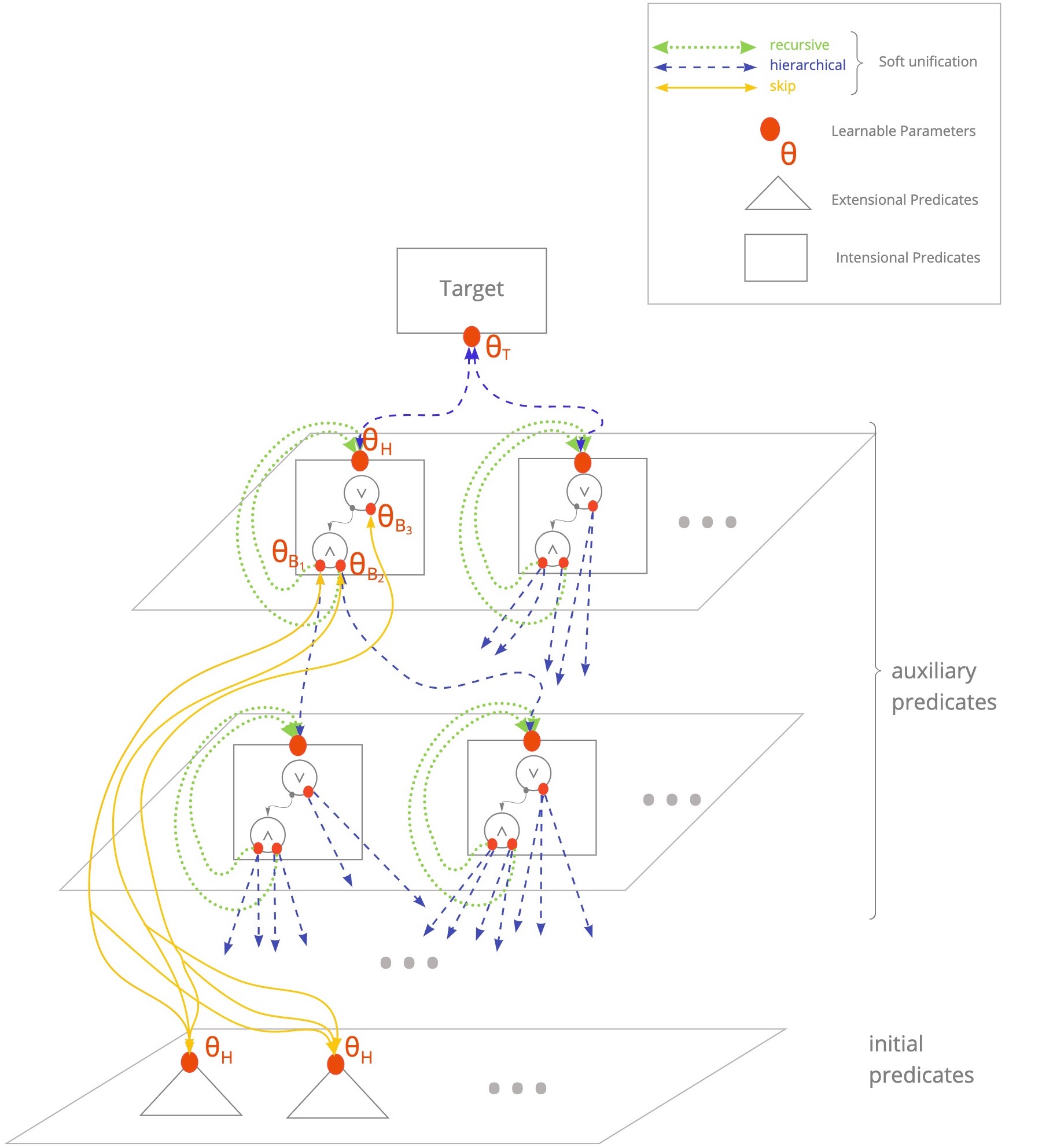
Figure 1: Hierarchical Model

Proto-rules

We first define the notion of proto-rules, which implicitly correspond to sets of meta-rules. A proto-rule is a meta-rule adaptive (see Appendix A for a formal definition). For instance, (3) extended as a proto-rule could be written as:

$$\mathrm{H}(X,Y)\leftarrow\overline{\mathrm{B}}_{1}(X,Z)\land\overline{\mathrm{B}}_{2}(Z,Y),$$ (7)

where the $\overline{\mathrm{B}}_{i}$’s correspond to predicate variables, of arity $2$ or $1$, where the second argument is optional. For instance, (7) can be instantiated as the following rule:

$$P(X,Y)\leftarrow P_{1}(X)\land P_{2}(Z,Y)$$ (8)

where $P$, $P_{2}$ are binary predicates, and $P_{1}$ is a unary predicate implicitly viewed as the binary predicate $\overline{P_{1}}$, where $\forall z,\overline{P_{1}}(x,z)\coloneqq P_{1}(x)$.

We propose a minimal and expressive set of proto-rules in Section 4.2. However, HRI can be instantiated with any set $\mathcal{R}$ of proto-rules. The choice of $\mathcal{R}$ defines the language bias used in the model.

Incremental Prior

To reinforce the incremental aspect of predicate invention, in contrast to LRI, each auxiliary predicate is directly associated with a unique proto-rule defining it. This has two advantages. First, it partially addresses the underestimation issue of (4) since it amounts to setting $\alpha_{P\mathrm{H}}=1$. Second, it reduces computational costs since the soft unification for a rule can be computed only by matching the body atoms. In order to preserve expressivity, we can re-introduce disjunctions in the model by considering proto-rules with disjunctions in their bodies (see Section 4.2); e.g., (7) could be extended to:

$$\mathrm{H}(X,Y)\leftarrow\big{(}\overline{\mathrm{B}}_{1}(X,Z)\land\overline{\mathrm{B}}_{2}(Z,Y)\big{)}\lor\overline{\mathrm{B}}_{3}(X,Y).$$ (9)

Hierarchical Prior

A hierarchical architecture is enforced by organizing auxiliary predicates in successive layers, from layer $1$ to the max layer $n_{L}$, as illustrated Figure 1 . Layer $0$ contains all input predicates. For each layer $l=1,\ldots,n_{L}$, each proto-rule in $\mathcal{R}$ generates one auxiliary predicate.

Lastly, the target predicate is matched with the auxiliary predicates in layer $n_{L}$ only.

With this hierarchical architecture, an auxiliary predicate $P$ at layer $\ell$ can be only defined from a set $\mathcal{P}_{\ell}^{\downarrow}$ of predicates at a layer lower or equal to $\ell$. This set can be defined in several ways depending on whether recursivity is allowed. We consider three cases: no recursivity, iso-recursivity, and full recursivity. For the no recursivity (resp. full recursivity) case, $\mathcal{P}_{\ell}^{\downarrow}$ is defined as the set $\mathcal{P}_{<\ell}$ (resp. $\mathcal{P}_{\leq\ell}$) of predicates at layer strictly lower than (resp. lower or equal to) $\ell$. For iso-recursivity, $\mathcal{P}_{\ell}^{\downarrow}$ is defined as $\mathcal{P}_{<\ell}\cup\{P\}$.

Enforcing this hierarchical prior has two benefits. First, it imposes a stronger language bias, which facilitates learning. Second, it also reduces computational costs since the soft unification does not need to consider all predicates.

Improved Model Inference

We improve LRI’s inference technique with a soft unification computation that reduces the underestimation issue in (4), which is due to the product of many values in $[0,1]$. For clarity’s sake, we illustrate the inference with proto-rule (9); although the equations can be straightforwardly adapted to any proto-rule. One inference step in our model is formulated as follows:

$$\begin{array}[]{ll}v_{and}&=\textsc{pool}_{\mathsf{P}_{1},\mathsf{P}_{2}}\left(\alpha_{P_{1}\mathrm{B}_{1}}\cdot\alpha_{P_{2}\mathrm{B}_{2}}\cdot\textsc{and}[v_{\mathsf{P}_{1}},v_{\mathsf{P}_{2}}]\right)\\ v_{or}&=\textsc{or}\left[v_{and},\textsc{pool}_{\mathsf{P}_{3}}\left(\alpha_{P_{3}\mathrm{B}_{3}}\cdot v_{\mathsf{P}_{3}}\right)\right]\\ v&=\textsc{merge}\left(v_{old},v_{or}\right),\end{array}$$ (10)

where $v$ (resp. $v_{old}$) denotes the new (resp. old) valuation of a grounded auxiliary predicate $\mathsf{P}$. For an auxiliary predicate at layer $\ell$, the pool operation is performed over both predicates $P_{1},P_{2},P_{3}\in\mathcal{P}_{\ell}^{\downarrow}$ and the groundings that are compatible to $\mathsf{P}$. However, before pooling, in presence of an existential quantifier as in proto-rule (9), a max is applied to the corresponding dimension of the tensor. The valuation $v^{t}$ of the target predicate (with variable denoted $\mathrm{P}^{t}$) is computed as a merge of its previous valuation $v^{t}_{old}$ and a pool over atoms at layer $n_{L}$:

$$v^{t}=\textsc{merge}\left(v^{t}_{old},\textsc{pool}_{\mathsf{P}_{1}}\left(\alpha_{P_{1}\mathrm{P}^{t}}\cdot v_{\mathsf{P}_{1}}\right)\right).$$ (11)

The underestimation issue is alleviated in two ways. First, the pool operation is implemented as a sum, and as $\min$, or as $\max$, and merge as $\max$. Second, the unification scores $\alpha_{P_{i}\mathrm{B}_{i}}$’s based on cosine are renormalized with a softmax transformation:

$$\alpha_{P_{i}\mathrm{B}_{i}}=\frac{\exp(\cos(\bm{\theta}_{P_{i}},\bm{\theta}_{\mathrm{B}_{i}})/\tau)}{\sum_{P_{j}}\exp(\cos(\bm{\theta}_{P_{j}},\bm{\theta}_{\mathrm{B}_{i}})/\tau)},$$ (12)

where $P_{j}\in\mathcal{P}_{\ell}^{\downarrow}$ and hyperparameter $\tau$, called temperature, controls the renormalization. Score $\alpha_{P_{1}\mathrm{P}^{t}}$ can be computed in a similar way with embedding $\bm{\theta}_{\mathrm{P}^{t}}$. These choices have been further experimentally validated (see Appendix B).

Equation (10) implies that the computational complexity of one inference step at layer $\ell$ if there is no recursion is $\mathcal{O}(n_{L}\times|\mathcal{P}_{\ell}|\times|\mathcal{P}_{\ell}^{\downarrow}|^{2}\times|\mathcal{C}|^{2})$ where $\mathcal{P}_{\ell}$ is the set of predicates at layer $\ell$ and $\mathcal{P}_{\ell}^{\downarrow}$ is the set of predicates available for defining an auxiliary predicate at layer $\ell$. Its spatial complexity at layer $\ell$ is $\mathcal{O}(n_{L}\times|\mathcal{P}_{\ell}|\times|\mathcal{C}|^{2})$.

The inference step described above is iterated $n_{I}$ times, updating the valuations of auxiliary and target predicates. Note that when recursive definitions of predicates are allowed, it could be conceivable to iterate this inference step until convergence. A nice property of this inference procedure is that it is parallelizable, which our implementation on GPU takes advantage of.

4.2 Generic Set of Proto-Rules

Although HRI is generic, we design a small set of expressive proto-rules to instantiate our model. We introduce first the following set of proto-rules $\mathcal{R}_{0}$ (see Figure 2):

$$\left\{\begin{array}[]{llllll}\mathfrak{A}:&\mathrm{H}(X)&\leftarrow&\overline{\mathrm{B}}_{1}(X,Y)&\land&\overline{\mathrm{B}}_{2}(Y,X)\\ \mathfrak{B}:&\mathrm{H}(X,Y)&\leftarrow&\overline{\mathrm{B}}_{1}(X,Z)&\land&\overline{\mathrm{B}}_{2}(Z,Y)\\ \mathfrak{C}:&\mathrm{H}(X,Y)&\leftarrow&\overline{\mathrm{B}}_{1}(X,Y)&\land&\overline{\mathrm{B}}_{2}(Y,X)\end{array}\right\}$$

where the $\overline{\mathrm{B}}_{i}$’s correspond to predicate variables where the second argument is optional (see Section 4.1).

(a) Meta-rule $\mathfrak{A}$	(b) Meta-rule $\mathfrak{B}$	(c) Meta-rule $\mathfrak{C}$

Figure 2: Three types of meta-rules: boxes represent variables, green arrows represent relations for head atoms and blue arrows represent relations for body atoms

To support our design, we analyzed the expressivity of $\mathcal{R}_{0}$, by investigating which fragment of first-order logic can be generated by $\mathcal{R}_{0}$ from a set of predicates $\mathcal{P}$. Because of space constraints, we only present here our main result, where we assume that $\mathcal{P}$ contains the zero-ary predicate $\mathtt{True}$ and the equality symbol:

Theorem 4.1.

The hypothesis space generated by $\mathcal{R}_{0}$ from $\mathcal{P}$ is exactly the set of function-free definite Horn clause fragment $\mathcal{F}_{\mathcal{P},\leq 2}^{\{1,2\}}$ composed of clauses with at most two body atoms involving unary and binary predicates in $\mathcal{P}$.

We refer the reader to Appendix A for all formal definitions, proofs and further theoretical results. This results implies that our model with $\mathcal{R}_{0}$ can potentially solve perfectly any ILP task whose target predicate is expressible in $\mathcal{F}_{\mathcal{P},\leq 2}^{\{1,2\}}$ with a large enough max layer $n_{L}$.

However, to potentially reduce the max layer $n_{L}$ and facilitate the definition of recursive predicates, we extend $\mathcal{R}_{0}$ to the set $\mathcal{R}_{0}^{\lor}$ by including a disjunction with a third atom in all the proto-rules:

$$\left\{\begin{array}[]{llllllll}\mathfrak{A}_{*}:&\mathrm{H}(X)&\leftarrow&\left(\overline{\mathrm{B}}_{1}(X,Y)\right.&\land&\left.\overline{\mathrm{B}}_{2}(Y,X)\right)&\vee&\overline{\mathrm{B}}_{3}(X,T)\\ \mathfrak{B}_{*}:&\mathrm{H}(X,Y)&\leftarrow&\left(\overline{\mathrm{B}}_{1}(X,Z)\right.&\land&\left.\overline{\mathrm{B}}_{2}(Z,Y)\right)&\vee&\overline{\mathrm{B}}_{3}(X,Y)\\ \mathfrak{C}_{*}:&\mathrm{H}(X,Y)&\leftarrow&\left(\overline{\mathrm{B}}_{1}(X,Y)\right.&\land&\left.\overline{\mathrm{B}}_{2}(Y,X)\right)&\vee&\overline{\mathrm{B}}_{3}(X,Y)\\ \end{array}\right\}$$

Moreover, as we have observed a certain redundancy to be beneficial to the learning, we incorporate the permutation rule $\mathfrak{I}$ in our experiments:

$$\mathcal{R}_{*}=\mathcal{R}_{0}^{\lor}\cup\{\mathfrak{I}:H(X,Y)\leftarrow\overline{F}(Y,X)\}$$

This small set of protorules $\mathcal{R}_{*}$, which has the same expressivity as $\mathcal{R}_{0}$ characterized in Theorem 4.1, is used to instantiate our model in all our experiments.

5 Proposed Training Method

Training

We train our model with a fixed number $n_{T}$ of training iterations. For each iteration, the model is trained using one training instance. During each iteration, we add a geometrically-decaying Gaussian-distributed noise to the embeddings for both predicates and rules to avoid local optima, similarly to LRI (Campero et al., 2018). Then the improved inference procedure described in (10) is performed with these noisy embeddings for a number $n_{I}$ of steps to get the valuations for all predicates. After these $n_{I}$ inference steps, the binary cross entropy (BCE) loss of the ground-truth target predicate valuation and the learned target predicate valuation is calculated:

$$\sum_{x,y}\scalebox{0.75}[1.0]{$-$}G^{t}_{x,y}\log\big{(}v(\mathsf{P}^{t}_{x,y})\big{)}-(1\scalebox{0.75}[1.0]{$-$}G^{t}_{x,y})\log\big{(}1\scalebox{0.75}[1.0]{$-$}v(\mathsf{P}^{t}_{x,y})\big{)},$$ (13)

where the sum is over all pairs of objects $x,y$ in one training instance, $G^{t}_{x,y}\in\{0,1\}$ is the ground truth value of atom $\mathsf{P}^{t}_{x,y}=P^{t}(x,y)$. To encourage the unification scores to be closer to $0$ or $1$, an extra regularisation term is added to the BCE loss to update the embeddings:

$$+\lambda\sum_{P,\mathrm{Q}}\alpha_{P\mathrm{Q}}\big{(}1-\alpha_{P\mathrm{Q}}\big{)}.$$ (14)

where hyperparameter $\lambda$ controls the regularization weight and the sum is over all predicates $P$ that can be matched with a predicate variable $\mathrm{Q}$ appearing in some meta-rules.

Task	$|I|$	Recursive	$\partial$ILP	LRI	Ours
					train	soft evaluation	symbolic evaluation
Predecessor	1	No	100	100	100	100	100
Undirected Edge	1	No	100	100	100	100	100
Less than	1	Yes	100	100	100	100	100
Member	1	Yes	100	100	100	100	100
Connectedness	1	Yes	100	100	100	100	100
Son	2	No	100	100	100	100	100
Grandparent	2	No	96.5	100	100	100	100
Adjacent to Red	2	No	50.5	100	100	100	100
Two Children	2	No	95	0	100	100	100
Relatedness	2	Yes	100	100	100	100	100
Cyclic	2	Yes	100	100	100	100	100
Graph Coloring	2	Yes	94.5	0	100	100	100
Even-Succ2	2	Yes	48.5	100	40	40	40
Buzz	2	Yes	35	70	100	40	40
Fizz	3	Yes	10	10	0	0	0

Table 1: Percentage of successful runs among 10 runs. $|I|$ is the smallest number of intensional predicates needed. Recursive means whether or not the solution needs to learn recursive rules.

In addition, to further help with convergence to an interpretable solution and avoid local optima, we replace during training the softmax transformation by a variant of Gumbel-softmax (Jang et al., 2017; Maddison et al., 2017). Commonly, it amounts to injecting a Gumbel noise $G_{j}$ in the softmax, i.e., in (12), we replace each $\cos(\bm{\theta}_{P_{j}},\bm{\theta}_{B_{i}})$ by $\cos(\bm{\theta}_{P_{j}},\bm{\theta}_{B_{i}})+G_{j}$ where Gumbel noise $G_{j}=-g\log\left(-\log\left(U_{j}\right)\right)$ is obtained by sampling $U_{j}$ according to a uniform distribution. However, we rely on a variant of this noise: $\tilde{G}_{j}=-g\log\left(-\log\left(U_{j}\right)\right)$, which is related as $\tilde{G}_{j}=\frac{\log(-\log g)}{g}G_{j}$. This choice has been experimentally favored. We discuss it further in the Appendix. Gumbel scale $g\in(0,+\infty)$ is linearly decreased during training. In contrast to the low-level parameter-noise applied directly to the embeddings, the Gumbel noise may be understood as a higher-level noise, enacted on the similarity coefficients themselves.

Convergence to an Interpretable Model

The passage from our soft model to a symbolic model may be realized by taking the limit of the softmax temperature in the unification score to zero, or equivalently, switching to an argmax in the unification score; i.e., for each proto-rule, the final learned rules can be interpreted by assigning head and body atoms to the predicates that obtain the highest unification score.

For instance, at a layer $\ell$, the extracted symbolic rule (8) could be extracted from proto-rule (7) if $P$ is the auxiliary predicate associated to that proto-rule at layer $\ell$ and

$$\left\{\begin{array}[]{ccc}P_{1}&=&\arg\max_{P\in\mathcal{P}^{\downarrow}_{\ell}}\>\alpha_{P\mathrm{B}_{1}}\\ P_{2}&=&\arg\max_{P\in\mathcal{P}^{\downarrow}_{\ell}}\>\alpha_{P\mathrm{B}_{2}}\end{array}\right.$$ (15)

Then we can interpret the solution by successively unfolding the logical formula extracted for each involved predicate, starting from the target predicate.

6 Experimental Results

We evaluated our model on multiple domains and compared with relevant baselines. In the main paper, for space constraints, we only present two sets of experiments. First, on standard ILP tasks, we show that our model is competitive against other neuro-symbolic methods in terms of performance, but also computational/space costs. Second, on a large domain from Visual Genome (Krishna et al., 2017), we show that our model can scale to a large multi-task problem and is superior to NLIL (Yang and Song, 2020).

Our results are averaged over several runs with different random seeds. In each run, the model is trained over a fixed number of iterations. Hyper-parameter details are given in Appendix D, and additional experiments (e.g., choice of operators, limitations of LRI, reinforcement learning) are discussed in Appendices B and C.

For simplicity and consistency, we instantiate our model with $\mathcal{R}_{*}$, with full recursivity in all the tasks except Visual Genome (no recursivity).

Note the performances can be improved and/or learning can be accelerated if we customize $\mathcal{R}_{*}$ to a task or restrict the recursivity. However, we intended to emphasize the genericity of our approach.

6.1 ILP Tasks

Task	#Training	% successful runs			Training time (secs)
	constants	NLM	DLM	Ours	NLM	DLM	Ours
Adjacent to Red	7	100	90	100	163	920	62
	10	90	90	100	334	6629	71
Grandparent	9	90	100	100	402	2047	79
	20	100	100	100	1441	3331	89

Table 2: Comparisons with NLM/DLM in terms of percentage of successful runs and average training times over 10 runs.

Model	Visual Genome
	R@1	R@5
MLP+RCNN	0.53	0.81
Freq	0.40	0.44
NLIL	0.51	0.52
Ours	0.53	0.60

Table 3: R@1 and R@5 for 150 objects classification on VG.

We evaluated our model on the ILP tasks from (Evans and Grefenstette, 2018), which are detailed in Appendix B, where we also provide the interpretable solutions found by our model.

We compare our model with $\partial$ILP (Evans and Grefenstette, 2018) and LRI (Campero et al., 2018) using their reported results. In contrast to LRI or $\partial$ILP, which use a specific set of meta-rules tailored for each task, we use the same generic and more expressive template set $\mathcal{R}_{*}$ to tackle all tasks; naturally, this generic approach impedes the learning for a few tasks.

A selection of the results on these ILP tasks are presented in Table 1 (see Appendix B). A run is counted as successful if the mean square error between inferred and given target valuations is less than 1e-4 for new evaluation datasets. Column train corresponds to the performance measured during training, while Column soft evaluation resp. symbolic evaluation to evaluation performance (no noise), using (11) resp. the interpretable solution (see end of Section 5).

We also ran our model on two other ILP tasks used by NLM (Dong et al., 2019) and DLM (Zimmer et al., 2021) to compare their performances and training times for a varying number of training constants. Those two ILP tasks are similar to those used in (Evans and Grefenstette, 2018), but with different background predicates. The results reported in Table 3 show that our model is one to two orders of magnitude faster and that it scales much better in terms of training constants, while achieving at least as good performances.

Initialization	Accuracy		Precision		R@1
	soft evaluation	symbolic evaluation	soft evaluation	symbolic evaluation	soft evaluation	symbolic evaluation
Random	0.63	0.49	0.57	0.5	0.23	0.38
NLIL	0.75	0.6	0.87	0.75	0.46	0.58
GPT2	0.65	0.45	0.72	0.66	0.27	0.5

Table 4: Performance of different embedding initializations for single Visual Genome task.

6.2 Visual Genome

Our model can be applied beyond classical ILP domains, and even benefit from richer environments and semantic structure. Futhermore, initial predicates embeddings can be boostrapped by visual or semantic priors. We illustrate it by applying it to the larger dataset of Visual Genome (Krishna et al., 2017), or more precisely a pre-processed (less noisy) version known as the GQA (Hudson and Manning, 2019a). Similarly to Yang and Song (2020), we filtered out the predicates with less than 1500 occurrences, which lead to a KB with 213 predicates; then, we solved ILP-like task to learn the explanations for the top 150 objects in the dataset. More details on task, results, baseline and metrics used are provided in Appendix C.

We ran a first set of experiments to validate that embeddings priors may be leveraged and compared three initialization methods: random initialization, pretrained embeddings from NLIL (Yang and Song, 2020), and pretrained embeddings from NLP model GPT2 (Radford et al., 2019). We trained our model on a single ILP task, which consists in predicting predicate Car. For this task, we further filtered the GQA dataset to keep 185 instances containing cars. Table 4 presents the accuracy, precision, and recall, obtained over 10 runs. Pretrained embeddings outperform the randomly initialized ones in all metrics. Embeddings from NLIL, trained specifically on this dataset, expectedly yield the best results. Although, to be fair, for the next experiments, we rely on the NLP embeddings.

In multitask setting, we trained 150 target models together with shared background predicate embeddings, where each model corresponds to one object classification. The training consists of $N_{r}$ rounds. In each round, we trained each model sequentially, by sampling for each target $n_{p}$ instances containing positive examples, and $n_{r}$ with or without positive examples.

We compared our model with NLIL (Yang and Song, 2020) and two other supervised baselines (classifiers) mentioned in their paper: Freq, which predicts object class by checking the related relation that contains the target with the highest frequency; and MLP-RCNN, a MLP classifier trained with RCNN features extracted from object images in Visual Genome dataset. The latter is a strong baseline because it uses visual information for its predictions while the other methods only use relational information. Like NLIL, we use R@1 and R@5 to evaluate the trained models. Table 3 summarizes the results. We see that both our method and MLP+RCNN achieve best performance for R@1. For R@5, we outperform Freq and NLIL. Table 5 shows some extracted learned rules for the multitask model.

Target	Rules
wrist	$\begin{aligned} wrist(X)&\leftarrow\left(watch(Y)\land on(Y,X)\right)\vee False\end{aligned}$
person	$\begin{aligned} person(X)&\leftarrow\left(on(X,Y)\land bench(Y)\right)\vee wearing(X,T)\end{aligned}$
vase	$\begin{aligned} vase(X)&\leftarrow\left(aux(X,Y)\land flowers(Y)\right)\vee False\\ aux(X,Y)&\leftarrow\left(True\land on(Y,X)\right)\vee with(X,Y)\end{aligned}$
logo	$\begin{aligned} logo(X)&\leftarrow\left(aux_{0}(X)\land True\right)\vee aux_{1}(X)\\ aux_{1}(X)&\leftarrow\left(on(X,Y)\land laptop(Y)\right)\vee False\\ aux_{0}(X)&\leftarrow\left(on(X,Y)\land kite(Y)\right)\vee False\end{aligned}$

Table 5: Examples of extracted rules from multi-task model

7 Ethical Considerations

Regarding our last experiment choice, let us point out that the use of data coming from annotated images, as well as the use of pretrained embeddings produced by the NLP model GPT2 should be regarded with circumspection. As it as been well documented (Papakyriakopoulos; Tommasi), such data holds strong biases, which would raise ethical issues when deployed in the real-world. Our motive was merely to illustrate the performance of our model in more noisy domains typical of real-world scenarios (such as autonomous driving scenarios). We strongly advise against the use of such unbiased data for any real-world deployement.

8 Conclusion

We presented a new neuro-symbolic interpretable model performing hierarchical rule induction through soft unification with learned embeddings; it is initialised by a theoretically supported small-yet-expressive set of proto-rules, which is sufficient to tackle many classical ILP benchmark tasks, as it encompasses a consequent function-free definite Horn clause fragment. Our model has demonstrated its efficiency and performance in both ILP, reinforcement learning (RL) and richer domains against state-of-the-art baselines, where it is typically one to two orders of magnitude faster to train.

As future work, we plan to apply it to broader RL domains (e.g., inducing game rules from a game trace) but also to continual learning scenarios where an interpretable logic-oriented higher-level policy would be particularly pertinent (e.g., autonomous driving). Indeed, we postulate that our model may be suited for continual learning in semantically-richer domains, for multiple reasons detailed in Appendix  E, alongside current limitations of our approach, which could be further investigated upon.

Appendix

A Expressivity Analysis

Many methods within inductive logic programming (ILP) define meta-rules, i.e., second-order Horn clauses which delineates the structure of learnable programs. The choice of these meta-rules, referred to as a language bias and restricting the hypothesis space, results in a well-known trade-off between efficiency and expressivity. In this section, we bring some theoretical justification for our designed set of second-order Horn Clause, by characterizing its expressivity. Relying on minimal sets of metarules for rule induction models has been shown to improve both learning time and predictive accuracies [Cropper and Muggleton, 2014, Fonseca et al., 2004]. For a model to be both adaptive and efficient, it seems pertinent to aim for a minimal set of meta-rules generating a sufficiently expressive subset of Horn clauses. The desired expressivity is ineluctably contingent to the tackled domain(s); a commonly-considered fragment is Datalog $\mathcal{D}$ which has been proven expressive enough for many problems. Datalog is a syntactic subset of Prolog which, by losing the Turing-completeness of Prolog/Horn, provides the undeniable advantage that its computations always terminate. Below, we focus our attention to similar fragments, in concordance with previous literature [Galárraga et al., 2013, Cropper and Tourret, 2020].

To make the document self-contained, before stating our results, let us introduce both concepts and notations related to First and Second Order Logic. Recall $\mathcal{P}$ denote the set of all considered predicates.

Horn Logic

We focus on Horn clause logic, since it is a widely adopted Turing-complete subset of FOL.

A Horn clause is a clause with at most one positive literal. Horn clauses may be of the following types (where $\mathsf{P}$, $\mathsf{Q}$, $\mathsf{T}$, and $\mathsf{U}$ are atoms):

• goal clauses which have no positive literal; they are expressed as $\lnot\mathsf{P}\lor\lnot\mathsf{Q}\lor...\lor\lnot\mathsf{T}$ or equivalently $\mathtt{False}\leftarrow\mathsf{P}\land\mathsf{Q}\land...\land\mathsf{T}$,

• definite clauses which have exactly one positive literal; they are expressed as $\lnot\mathsf{P}\lor\lnot\mathsf{Q}\lor...\lor\lnot\mathsf{T}\lor\mathsf{U}$ or equivalently as a Horn rule $\mathsf{U}\leftarrow\mathsf{P}\land\mathsf{Q}\land...\land\mathsf{T}$,

• facts which can be expressed as $\mathsf{U}\leftarrow\mathtt{True}$ where $\mathsf{U}$ is grounded.

Meta-rules

We follow the terminology from the Meta Interpretative Learning literature [Cropper and Tourret, 2020]:

Definition 8.1.

A meta-rule is a second-order Horn clause of the form: $A_{0}\leftarrow A_{1}\land...\land A_{m}$ where each $A_{i}$ is a literal of the form $P(T_{1},...,T_{n_{i}})$ where $P$ is a predicate symbol or a second-order variable that can be substituted by a predicate symbol, and each $T_{i}$ is either a constant symbol or a first-order variable that can be substituted by a constant symbol.

Here are some examples of intuitive meta-rules, which will be of later use:

$$\begin{array}[]{lllll}(\sigma)&\mathrm{P}(A,B)&\leftarrow&\mathrm{Q}(B,A)&permute\\ (\iota)&\mathrm{P}(A,B)&\leftarrow&\mathrm{Q}(A)&expand\\ (\exists)&\mathrm{P}(A)&\leftarrow&\exists B,\mathrm{Q}(A,B)&existential\>contraction\\ (\forall)&\mathrm{P}(A)&\leftarrow&\forall B,\mathrm{Q}(A,B)&universal\>contraction\\ (\nabla)&\mathrm{P}(A)&\leftarrow&\mathrm{Q}(A,A)&diagonal\>extract\\ (\Delta)&\mathrm{P}(A,A)&\leftarrow&\mathrm{Q}(A)&diagonal\>fill\\ \end{array}$$ (16)

A common meta-rule set, which has been used and tested in the literature [Cropper and Tourret, 2020], is the following:

$$\mathcal{R}_{MIL}=\left\{\begin{array}[]{lllll}(\texttt{Indent}_{1})&&\mathrm{P}(A)&\leftarrow&\mathrm{Q}(A)\\ (\texttt{DIndent}_{1})&&\mathrm{P}(A)&\leftarrow&\mathrm{Q}(A)\land\mathrm{R}(A)\\ (\texttt{Indent}_{2})&&\mathrm{P}(A,B)&\leftarrow&\mathrm{Q}(A,B)\\ (\texttt{DIndent}_{2})&&\mathrm{P}(A,B)&\leftarrow&\mathrm{Q}(A,B)\land\mathrm{R}(A,B)\\ (\texttt{Precon})&&\mathrm{P}(A,B)&\leftarrow&\mathrm{Q}(A)\land\mathrm{R}(A,B)\\ (\texttt{Postcon})&&\mathrm{P}(A,B)&\leftarrow&\mathrm{Q}(A,B)\land\mathrm{R}(B)\\ (\texttt{Curry})&&\mathrm{P}(A,B)&\leftarrow&\mathrm{Q}(A,B,\mathrm{R})\\ (\texttt{Chain})&&\mathrm{P}(A,B)&\leftarrow&\mathrm{Q}(A,C)\land\mathrm{R}(C,B)\\ \end{array}\right\}$$ (17)

where the letters $\mathrm{P},\mathrm{Q},\mathrm{R}$ correspond to existentially-quantified second-order variables and the letters $A,B,C$ to universally-quantified first-order variables.

Proto-rules

Our model relies on an extended notion of meta-rules, which we refer to as proto-rules. These templates have the specificity that they do not fix the arity of their body predicates; only the arity of the head predicate is determined. Formally, they can be defined as follows. For any $n\in\mathbb{N}$, let $\mathcal{P}^{n}$ (resp. $\mathcal{P}^{\leq n}$) be the predicates in $\mathcal{P}$ that have arity equal to (resp. lower or equal to) $n$.

Define the projection operator $\nu^{n}$ which canonically embeds predicates of arity $i\leq n$ in the space of predicates of arity $n$:

$$\nu^{n}:\mathcal{P}^{\leq n}\longrightarrow\mathcal{P}^{n}\quad\text{ s.t. }\quad\nu^{n}(P)(X_{1},\cdots,X_{n})=P(X_{1},\cdots,X_{i})\text{ for }P\in\mathcal{P}^{i}.$$ (18)

Note that the restriction of $\nu^{n}$ on the space of predicates of arity n is identity: $\nu^{n}\mid_{\mathcal{P}^{n}}=id_{\mathcal{P}^{n}}$. Moreover, this projection naturally extends to second-order variables. To ease the notations, we denote below the projection $\nu^{n_{i}}$ with an overline (e.g., for a predicate $P$, $\nu^{n_{i}}(P)=\overline{P}$), since there is no risk of confusion because $n_{i}$ is specified by its arguments $(T_{1},\ldots,T_{n_{i}})$.

Definition 8.2.

A proto-rule is an extension of a second-order Horn clause of the form: $A_{0}\leftarrow A_{1}\land\ldots\land A_{m}$, where $A_{0}$ (resp. each $A_{i},i>0$ is a literal of the form $P(T_{1},...,T_{n_{i}})$ (resp. $\nu^{n_{i}}\big{(}{P}\big{)}(T_{1},...,T_{n_{i}})$ in which $P$, which is a predicate symbol or a second-order variable that can be substituted by a predicate symbol, is of arity lower or equal to $n_{i}$, and each $T_{i}$ is either a constant symbol or a first-order variable that can be substituted by a constant symbol.

Seeing second-order rules as functions over predicate spaces to first-order logic rules, we can provide another characterization of proto-rules: a meta-rule can be understood as a mapping $\mathcal{P}^{n_{1}}\times\ldots\times\mathcal{P}^{n_{m}}\rightarrow\mathcal{H}$ for some indices $n_{i}$, i.e., taking $m$ predicates of specific arities and returning a first-order Horn clause; in contrast, a proto-rule is a mapping $\mathcal{P}^{\leq n_{1}}\times\ldots\times\mathcal{P}^{\leq n_{m}}\rightarrow\mathcal{H}$, for some indices $n_{i}$.

The first set of protorules we propose is the following:

$$\mathcal{R}_{0}:=\left\{\begin{array}[]{llll}\mathfrak{A}:&P(A)&\leftarrow&\overline{Q}(A,B)\land\overline{R}(B,A)\\ \mathfrak{B}:&P(A,B)&\leftarrow&\overline{Q}(A,C)\land\overline{R}(C,B)\\ \mathfrak{C}:&P(A,B)&\leftarrow&\overline{Q}(A,B)\land\overline{R}(B,A)\\ \end{array}\right\}$$ (19)

Horn Fragments

A Horn theory $\mathcal{T}$ is a set of Horn clauses.

Let us denote the set of second order Horn clause, the set of definite Horn clauses, and the set of function-free definite Horn clauses respectively by $\mathcal{H}$, $\mathcal{S}$, and $\mathcal{F}$. Within Horn clause logic, several restrictions have been proposed in the literature to narrow the hypothesis space, under the name of fragment. A fragment is a syntactically restricted subset of a theory. Following previous work (such as [Cropper and Tourret, 2020]), we introduce below a list of classic fragments of $\mathcal{F}$, in decreasing order:

• connected fragment, $\mathcal{C}$: connected definite function-free clauses, i.e., clauses in $\mathcal{F}$ whose literals can not be partitioned into two sets such that the variables attached to one set are disjoint from the variables attached to literals in the other set; e.g., $P(A,B)\leftarrow Q(A,C)\land R(A,B)$ is connected while the following clause is not $P(A,B)\leftarrow Q(A,C)\land R(B)$.

• Datalog fragment, $\mathcal{D}$: sub-fragment of $\mathcal{C}$, composed of clauses such that every variable present in the head of the Horn rule also appears in its body.

• two-connected fragment, $\mathcal{K}$: sub-fragment of $\mathcal{D}$ composed of clauses such that the variables appearing in the body must appear at least twice.

• exactly-two-connected fragment, $\mathcal{E}$: sub-fragment of $\mathcal{K}$ such that the variables appearing in the body must appear exactly twice.

• duplicate-free fragment, $\mathcal{U}$: sub-fragment of $\mathcal{K}$ excluding clauses in which a literal contains multiple occurrences of the same variable, e.g., excluding $P(A,A)\leftarrow Q(A)$.

These fragments are related as follows:

$$\mathcal{H}\supset\mathcal{S}\supset\mathcal{F}\supset\mathcal{C}\supset\mathcal{D}\supset\mathcal{K}\begin{array}[]{c}\rotatebox[origin={c}]{25.0}{$\supset$}\hskip 5.0pt\mathcal{E}\\ \rotatebox[origin={c}]{-25.0}{$\supset$}\hskip 5.0pt\mathcal{U}\end{array}$$ (20)

For $\mathcal{M}$ a set of meta-rules, we denote $\mathcal{M}^{\leq a}_{\leq m}$ the fragment of $\mathcal{M}$ where each literal has arity at most $a$ and each meta-rule has at most $m$ body literals. We extend the notation in order to allow both $a$ and $m$ to be a set of integers; e.g., $\mathcal{M}^{\{1,2\}}_{\{3\}}$ is the fragment of $\mathcal{M}$ where each literal corresponds to an unary or binary predicate and the body of each meta-rule contains exactly three literals.

Binary Resolution

As it would be of future use, let us introduce some notions around resolution. To gain intuition about the notion of resolvent, let us look at an example before stating more formal definitions. Consider the following Horn clauses:

$$\begin{array}[]{llll}C_{1}:&P(X,Y)\lor\lnot Q(X)\lor\lnot R(X,Y)&\text{ or, equivalently, }&P(X,Y)\leftarrow Q(X)\land R(X,Y)\\ C_{2}:&R(X,a)\lor\lnot T(X,a)\lor\lnot S(a)&\text{ or, equivalently, }&R(X,a)\leftarrow S(a)\land T(X,a)\end{array}$$

The atoms $R(X,Y)$ and $R(X,a)$ are unifiable, under the substitution $\sigma:\{a/Y\}$; under this substitution, we obtain the following clauses:

$$\{P(X,a)\lor\lnot Q(X)\lor\lnot R(X,a),R(X,a)\lor\lnot T(X,a)\lor\lnot S(a)\}$$

Since either $R(X,a)$ is True, or $\lnot R(X,a)$ is True, assuming $C_{1}$ and $C_{2}$ are True, we can deduce the following clause is True:

$$(P(X,a)\lor\lnot Q(X))\lor(\lnot T(X,a)\lor\lnot S(a))\text{ or, equivalently, }P(X,a)\leftarrow Q(X)\land T(X,a)\land S(a)$$

This resulting clause, is a binary resolvent of $C_{1}$ and $C_{2}$.

Now, let us state more formal definitions. We denote $\sigma=\{t_{1}/X_{1},\cdots,t_{n}/X_{n}\},$ a substitution and $E\sigma$ the expression obtained from an expression $E$ by simultaneously replacing all occurrences of the variables $X_{i}$ by the terms $t_{i}$.

Definition 8.3.

• A substitution $\sigma$ is called a unifier of a given set of expressions $\{E_{1},\cdots,E_{m}\}$ , $m\geq 2$ if $E_{1}\sigma=\cdots=E_{m}\sigma$.

• A unifier $\theta$ of a unifiable set of expressions $E=\{E_{1},\cdots,E_{m}\}$ , $m\geq 2$, is said to be a most general unifier if for each unifier $\sigma$ of E there exists a substitution $\lambda$ such that $\sigma=\theta\lambda$.

Definition 8.4.

Consider two parent clauses $C_{1}$ and $C_{2}$ containing the literals $l_{1}$ and $l_{2}$ respectively. If $l_{1}$ and $\lnot l_{2}$ have a most general unifier $\sigma$, then the clause $(C_{1}\sigma\setminus l_{2}\sigma)\lor(C_{2}\sigma\setminus l_{2}\sigma)$ is called a binary resolvent of $C_{1}$ and $C_{2}$.

Derivation Reduction

Diverse reductions methods have been proposed in the literature, such as subsumption [Robinson, 1965], entailment [Muggleton, ], and derivation [Cropper and Tourret, 2018]. As previously pointed out (e.g., [Cropper and Tourret, 2020]), common entailment methods may be too strong and remove useful clauses enabling to make predicates more specific. The relevant notion to ensure the reduction would not affect the span of our hypothesis space is the one of derivation-reduction (D-reduction) [Cropper and Tourret, 2018], as defined in Definition 8.6.

Let us first define for the following operator for a Horn theory $\mathcal{T}$:

$$\left\{\begin{array}[]{lll}R_{0}(\mathcal{T})&=&\mathcal{T}\\ R_{n}(\mathcal{T})&=&\{C\mid C\text{ is the binary resolvent of }C_{1}\text{ and }C_{2}\text{ with }C_{1}\in R_{n-1}(\mathcal{T}),C_{2}\in\mathcal{T}\}\end{array}\right.$$

Definition 8.5.

The Horn closure of a Horn theory $\mathcal{T}$ is: $\displaystyle R^{\ast}(\mathcal{T})=\cup_{n}R_{n}(\mathcal{T})$.

Definition 8.6.

• A Horn clause $C$ is derivationally redundant in the Horn theory $\mathcal{T}$ if $\mathcal{T}\vdash C$, i.e., $C\in R^{\ast}(\mathcal{T})$; it is said to be $k$-derivable from $\mathcal{T}$ if $C\in R^{k}(\mathcal{T})$.

• A Horn theory $\mathcal{T}$ is derivationally reduced ($D$-reduced) if and only if it does not contain any derivationally redundant clauses.

A clausal theory may have several D-reductions. For instance, we can easily see that

$$\left\{\begin{array}[]{llll}C_{1}:&P(A,B)&\leftarrow&Q(B,A)\\ C_{2}:&P(A,B)&\leftarrow&Q(A,C),R(C,B)\\ C_{3}:&P(A,B)&\leftarrow&Q(A,C),R(B,C)\end{array}\right\}\text{ may be D-reduced to either }\{C_{1},C_{2}\}\text{ or }\{C_{1},C_{3}\}$$

Hypothesis Space

Recall that $\mathcal{P}$ (resp. $\mathcal{P}_{0}$) denotes the set of predicates (resp. of initial predicates); and $\mathcal{B}$ the background knowledge, may encompass both initial predicates and pre-given rules. As we are interested in characterizing the expressivity of our model, let us define the relevant notion of hypothesis space, which could apply to any rule-induction model attached to at meta-rule or proto-rule set:

Definition 8.7.

Given a predicate set $\mathcal{P}$, and a meta-rule or proto-rule set $\mathcal{M}$, let us define:

• the set $\mathcal{M}_{\mathcal{P}}$ as the set of all Horn clauses generated by all the possible substitutions of predicates variables in $\mathcal{M}$ by predicates symbols from $\mathcal{P}$.

• the hypothesis space $\mathcal{M}[\mathcal{P}]$ generated by $\mathcal{M}$ from $\mathcal{P}$ as the Horn closure of $\mathcal{M}_{\mathcal{P}}$.

Equality Assumption

The Equality relation is typically assumed part of FOL, so it is reasonable to assume it belongs to the background knowledge in our results below. In our approach, it amounts to integrating the predicate $\mathtt{Equal}$ to the set of initial predicates $\mathcal{P}_{0}$; $\mathtt{Equal}$, which corresponds to the identity, is intensionally defined on any domain $\mathbb{D}$ by:

$$\mathtt{Equal}:\left\{\begin{array}[]{lll}\mathbb{D}\times\mathbb{D}&\rightarrow&\mathbb{B}=\{\mathtt{True},\mathtt{False}\}\\ (X,Y)&\mapsto&\left\{\begin{array}[]{ll}\mathtt{True}&\text{ if }X=Y\\ \mathtt{False}&\text{ if }X\neq Y\end{array}\right.\end{array}\right.$$ (21)

Main Result

Here is our main result, concerning the investigation of the expressivity of the minimal set $\mathcal{R}_{0}$:

Theorem 8.8.

1. Assuming $\mathtt{True}\in\mathcal{P}_{0}$, the hypothesis space generated by $\mathcal{R}_{0}$ from $\mathcal{P}$ encompasses the set of duplicate-free and function-free definite Horn clause composed of clauses with at most two body atoms involving unary and binary predicates in $\mathcal{P}$:

   $$\mathtt{True}\in\mathcal{P}_{0}\implies\mathcal{R}_{0}[\mathcal{P}]\supset\mathcal{U}_{\leq 2}^{\{1,2\}}[\mathcal{P}]$$

2. Assuming $\mathtt{True},\mathtt{Equal}\in\mathcal{P}_{0}$, the hypothesis space generated by $\mathcal{R}_{0}$ from $\mathcal{P}$ corresponds to the set of function-free definite Horn clause composed of clauses with at most two body atoms involving unary and binary predicates in $\mathcal{P}$; i.e., in terms of the second order logic fragment:

   $$\mathtt{True},\mathtt{Equal}\in\mathcal{P}_{0}\implies\mathcal{R}_{0}[\mathcal{P}]=\mathcal{F}_{\leq 2}^{\{1,2\}}[\mathcal{P}]$$

We refer to the end of this section for the proof of this theorem.

Theorem 8.8 allows us to conclude that $\mathcal{R}_{0}$ is more expressive than the set commonly found in the literature $\mathcal{R}_{MIL}$, assuming we are working with predicates of arity at most $2$:

Corollary 8.9.

Assuming the initial predicates $\mathcal{P}_{0}$ contains only predicates of arity at most $2$, the hypothesis space generated by $\mathcal{R}_{0}$ given $\mathcal{P}$ encompasses the one generated by $\mathcal{R}_{MIL}$ as defined in (17).

$$\forall P\in\mathcal{P}_{0},\quad\mathrm{arity}(P)\leq 2\implies\mathcal{R}_{0}[\mathcal{P}]\supset\mathcal{R}_{MIL}[\mathcal{P}]$$

Proof.

Under our assumption, the meta-rule $(\texttt{Curry})$ in (17) may be disregarded. The remaining meta-rules present in $\mathcal{R}_{MIL}$ have already been examined in Theorem 8.8. $\mathcal{R}_{0}$ has therefore at least the same expressivity than $\mathcal{R}_{MIL}$. In order to be able to conclude $\mathcal{R}_{0}$ is strictly more expressive, we can mention the rules $P(A)\leftarrow P(A,B)$ or $P(A,B)\leftarrow P(B,A)$, which are reached by $\mathcal{R}_{0}$ not $\mathcal{R}_{M}IL$. ∎

Disjunction

In our model, to ensure an incremental learning of the target rule, we impose the restriction that each auxiliary predicate corresponds to one rule. Since such constraint risk to remove the possibility of disjunction, we redefine new proto-rules versions integrating disjunctions:

$$\mathcal{R}_{0}^{\lor}=\left\{\begin{array}[]{llll}\mathfrak{A}:&P(A)&\leftarrow&\left(\overline{Q}(A,B)\land\overline{R}(B,A)\right)\lor\overline{S}(A,B)\\ \mathfrak{B}:&P(A,B)&\leftarrow&\left(\overline{Q}(A,C)\land\overline{R}(C,B)\right)\lor\overline{S}(A,B)\\ \mathfrak{C}:&P(A,B)&\leftarrow&\left(\overline{Q}(A,B)\land\overline{R}(B,A)\right)\lor\overline{S}(A,B)\\ \end{array}\right\}$$ (22)

Adopting the minimal set $\mathcal{R}_{0}^{\lor}$, in our incremental setting does not affect the expressivity of the hypothesis space compared to when relying on the set $\mathcal{R}_{0}$ in a non incremental setting. Let us remind an incremental setting imposes a predicate symbol to be the head of exactly one rule.

Lemma 8.10.

The minimal proto-rule set $\mathcal{R}_{0}^{\lor}$ in an incremental setting holds the same expressivity as $\mathcal{R}_{0}$.

Proof.

It is straightforward to see that $\mathcal{R}_{0}^{\lor}$ is a minimal set.
The hypothesis space generated by $\mathcal{R}_{0}$ obviously encompasses the hypothesis space generated by $\mathcal{R}_{0}^{\lor}$ in an incremental setting. Reciprocally, let us assume $n$ rules instantiated from $\mathcal{R}_{0}$ are attached to one predicate symbol $P$. They can be expressed as:

$$\begin{array}[]{ccc}P(X,Y)&\leftarrow&f_{1}(X,Y)\\ P(X,Y)&\leftarrow&f_{2}(X,Y)\\ \cdots&\cdots&\cdots\\ P(X,Y)&\leftarrow&f_{n}(X,Y)\\ \end{array}$$

Recursively, we can define $P_{i}$ auxiliary predicates in the hypothesis space of $\mathcal{R}_{0}^{\lor}$.

$$\begin{array}[]{ccc}P_{1}(X,Y)&\leftarrow&f_{1}(X,Y)\\ P_{2}(X,Y)&\leftarrow&P_{1}(X,Y)\lor f_{2}(X,Y)\\ \cdots&\cdots&\cdots\\ P_{n}(X,Y)&\leftarrow&P_{n-1}(X,Y)\lor f_{n}(X,Y)\\ \end{array}$$

Since $P_{n}$ is then equivalent to $P$, we can conclude.

∎

Redundancy

Since we have observed a certain redundancy to be beneficial to the learning, we incorporate the permutation rule $\mathfrak{I}$ in our experiments, and rely on the following set:

$$\mathcal{R}_{*}=\mathcal{R}_{0}^{\lor}\cup\{\mathfrak{I}:H(X,Y)\leftarrow\overline{F}(Y,X)\}$$

This small—yet non minimal—set of protorules $\mathcal{R}_{*}$, has the same expressivity as $\mathcal{R}_{0}$ (characterized in Theorem 8.8)

Lemma 8.11.

The proto-rule set $\mathcal{R}_{\ast}$ holds the same expressivity than $\mathcal{R}_{0}$.

Proof.

It stems from the fact, observed in the proof of Theorem 8.8 that the rule $(\sigma)$, equivalent to $(\mathfrak{I})$ can be D-reduced from $\mathcal{R}_{0}$. ∎

Recursivity

The development of Recursive Theory arose first around the Hilbert’s Program and Gödel’s proof of the Incompleteness Theorems (1931) and is tightly linked to questions of computability. While implementing recursive-friendly model, we should keep in mind considerations of computability and decidability. Enabling full recursivity within the templates is likely to substantially affect both the learning and the convergence, by letting room to numerous inconsistencies.

With this in mind, let us consider different stratifications in the rule space, and in our model. First, we introduce a hierarchical filtration of the rule space: initial predicates are set of layer 0, and auxiliary predicates in layer $\ell$ are defined from predicates from layers at most $\ell$. Within such stratified space, different restrictions may be considered:

• recursive-free hierarchical hypothesis space:, where rules of layer $\ell$ are defined from rules of strictly lower layer. The proto-rules from $\mathcal{R}_{0}^{\lor}$ are therefore restricted to the following form:

  $$P(\cdot)\leftarrow\left[Q(\cdot)\land R(\cdot)\right]\lor O(\cdot),$$

  with $P\in\mathcal{P}_{\ell}$, $Q,R,O\in\mathcal{P}_{<\ell}$.

• iso-recursive hierarchical hypothesis space, where the only recursive rules allowed from $\mathcal{R}_{0}^{\lor}$ have the form:

  $$P(\cdot)\leftarrow\left[Q(\cdot)\land R(\cdot)\right]\lor O(\cdot),\quad\text{ with }P\in\mathcal{P}_{\ell},Q,R\in\mathcal{P}_{<\ell}\cup\{P\},O\in\mathcal{P}_{<\ell}$$

  Such space fits most recursive ILP tasks (e.g., Fizz, Buzz, Even, LessThan).

• recursive hierarchical hypothesis space, where the recursive rules allowed from $\mathcal{R}_{0}^{\lor}$ have the form:

  $$P(\cdot)\leftarrow\left[Q(\cdot)\land R(\cdot)\right]\lor O(\cdot)\quad\text{ with }P\in\mathcal{P}_{\ell},Q,R\in\mathcal{P}_{\leq\ell},O\in\mathcal{P}_{\leq\ell}.$$

  Such space is required for the recursivity present in EvenOdd or Length. Such hierarchical notion is also present in the Logic Programming literature under the name of stratified programs.

Proof of Theorem 8.8

Before we present the proof, let us introduce two additional notations:

• $\mathfrak{R}\prescript{}{i}{\odot}\mathfrak{R}^{\prime}$ refers to the resolvent of $\mathfrak{R}$ with $\mathfrak{R^{\prime}}$, where the $i^{th}$ body member of $\mathfrak{R}$ is resolved with the head of $\mathfrak{R}^{\prime}$. To illustrate it, consider the following meta-rules:

  $$\begin{array}[]{lc}\mathfrak{R}:&P(A)\leftarrow Q(A)\land R(A,B)\\ \mathfrak{R}^{\prime}:&P(A)\leftarrow Q(A)\land R(B,A)\\ \mathfrak{R}^{\prime\prime}:&P(A,B)\leftarrow Q(B,A)\end{array}$$

  The resolvent $\mathfrak{R}^{\prime}\prescript{}{2}{\odot}\mathfrak{R}^{\prime\prime}$ corresponds to resolve the second body atom of $\mathfrak{R}^{\prime}$ with $\mathfrak{R}^{\prime\prime}$, which therefore leads to $\mathfrak{R}$.

• We define the operation $\rho$ as the composition of a projection $\nu$, a permutation $(\sigma)$, and an existential contraction over the second variable $(\exists)$, which amounts to:

  $$\rho(R)(X):=\exists\circ\sigma(\overline{R}(X,Y))=\exists YR(Y)$$ (23)

  Here, we identified the permutation clause $(\sigma)$ (as defined in (16)) with the operation it defines on predicates $\sigma$; similarly for the existential clause $(\exists)$ with the contraction operation $\exists$.

  Likewise, we can define the corresponding non-connected meta-rule attached to the operation $\rho$ by:

  $$(\rho):\>P(X)\leftarrow\exists YR(Y)$$ (24)

Proof.

The inclusion $\mathcal{R}_{0}[\mathcal{P}]\subset\mathcal{F}_{\leq 2}^{\{1,2\}}[\mathcal{P}]$ is trivial since all the rules instantiated from $\mathcal{R}_{0}$ are definite Horn clause with two body predicates, and duplicate-free; similarly, if adding the duplicate-free constraint to $\mathcal{F}$ (and denoting it by $\mathcal{F}^{D}$), we can trivially state: $\mathcal{R}_{0}[\mathcal{P}]\subset\mathcal{F}_{\leq 2}^{D,\{1,2\}}[\mathcal{P}]$.

It remains to prove the other inclusion; e.g., for $(ii)$, it amounts to $\mathcal{R}_{0}[\mathcal{P}]\supset\mathcal{F}_{\leq 2}^{\{1,2\}}[\mathcal{P}]$, which boils down to $\mathcal{R}_{0}[\mathcal{P}]\supset\mathcal{F}_{\mathcal{P},\leq 2}^{\{1,2\}}$ since $\mathcal{R}_{0}[\mathcal{P}]$ is closed under resolution. We will proceed by successively extending the sub-fragments $\mathcal{M}$ we are considering while proving $\mathcal{R}_{0}[\mathcal{P}]\supset\mathcal{M}_{\mathcal{P}}$. For instance, under the assumption $\mathtt{True},\mathtt{Equal}\in\mathcal{P}_{0}$, we demonstrate that the hypothesis space generated by $\mathcal{R}_{0}$ encompasses the one generated by the increasingly larger fragments: (a) $\mathcal{U}$ (b) $\mathcal{K}$; (c) $\mathcal{D}$; (d) $\mathcal{C}$; (e) $\mathcal{F}$. For $(i)$, under the simpler assumption $\mathtt{True}\in\mathcal{P}_{0}$, we can follow almost identical steps, although the duplicate-free constraint can not be lifted, and therefore step $(b)$ is skipped. Since the proof of $(i)$ is more or less included in the proof of $(ii)$, we will below focus only on proving $(ii)$.

For each fragment $\mathcal{M}$, to demonstrate such inclusion, we can simply show that every rule within the fragment $\mathcal{M}_{\mathcal{P}}$ belongs to the hypothesis space generated by $\mathcal{R}_{0}$; more specifically, we will mostly work at the level of second order logic; there, we will show that any meta-rule in $\mathcal{M}$ can be reduced from meta-rules in $\mathcal{R}_{0}$, or generated by $\mathcal{R}_{0}$.

However, to avoid listing all the meta-rules generating these fragments, and restrict our enumeration, we leverage several observations: first, since we assume the predicate set includes $\mathtt{True}$, we can restrict our attention to clauses with exactly two body literals; secondly, the permutation meta-rule $(\sigma)$ (introduced in 16) can be derived from the proto-rule $\mathfrak{C}$ upon matching the first body in $\mathfrak{C}$ with $\mathtt{True}$; therefore, we can examine rules only upon permutation $(\sigma)$ applied to their body or head predicates.

1. First, let us demonstrate the following inclusion:

   $$\mathtt{Claim}_{1}:\quad\mathtt{True}\in\mathcal{P}_{0}\implies\mathcal{R}_{0}[\mathcal{P}]\supset\mathcal{U}_{\mathcal{P},\leq 2}^{\{1,2\}}$$ (25)

   By the previous observations, we can narrow down to examine a subset of the meta-rules generating $\mathcal{U}_{\leq 2}^{\{1,2\}}$, as listed and justified below. Our claim is that all these clauses are derivationally redundant from the Horn theory generated by $\mathcal{R}_{0}$; for each of them, we therefore explicit the clauses used to reduce them.
   

   $$\begin{array}[]{clll}&\text{ Meta-Rules }&\text{Reduction}&\text{Comment}\\ (i)&P(A)\leftarrow Q(A)\land R(A)&\mathfrak{A}\prescript{}{2}{\odot}\sigma&\mathfrak{A}(Q,\sigma(R))\\ (ii)&P(A)\leftarrow Q(A)\land R(A,B)&\mathfrak{A}\prescript{}{2}{\odot}\sigma&\mathfrak{A}(Q,\sigma(R))\\ (iii)&P(A)\leftarrow Q(A,B)\land R(B)&\mathfrak{A}&\\ (iv)&P(A)\leftarrow Q(A,B)\land R(B,A)&\mathfrak{A}&\\ (v)&P(A)\leftarrow Q(A,B)\land R(B,C)&\mathfrak{A}&\\ (vi)&P(A,B)\leftarrow Q(A)\land R(A,B)&\mathfrak{A}\prescript{}{2}{\odot}\sigma&\mathfrak{C}(Q,\sigma(R))\\ (vii)&P(A,B)\leftarrow Q(A,C)\land R(C,B)&\mathfrak{B}&\\ (viii)&P(A,B)\leftarrow Q(A,B)\land R(B,A)&\mathfrak{C}&\\ (ix)&P(A,B)\leftarrow Q(A,B)\land R(B,C)&\mathfrak{A}\prescript{}{2}{\odot}\exists&\mathfrak{A}(Q,\exists(R))\\ \end{array}$$

   Beside the notation of the resolvent $\odot_{H}$ explained previously, we provided a more intuitive form for the resolution (under ’Comment’), in terms of composition between maps, where we identify a proto-rule (or meta-rule) with a map of the following form:

   $$\mathcal{P}^{\bullet}\times\cdots\times\mathcal{P}^{\bullet}\rightarrow\mathcal{P}^{\bullet}$$

   Let us justify why these clauses are the only clauses in $\mathcal{U}_{\leq 2}^{\{1,2\}}$ worth to examine in two steps:

   • Let us consider clauses whose head predicate arity is $1$. First, by the Datalog assumption, we can indeed restrict our attention to body clauses where $A$ is appearing at least once. By symmetry, we can assume $A$ appears in the first body. By the connected assumption, either $A$ appears in the second body too, and/or an existential variable (say $B$) appears both in the first or second body. Upon permutation, it leads us to clauses $(i)-(v)$.

   • Let us consider clauses whose head predicate arity is $2$. First, by the Datalog assumption, we can indeed restrict our attention to body clauses where $A$ and $B$ have to appear at least once. The only body clause of arity $(1,1)$ satisfying this condition is not connected ($Q(A)\land R(B)$); upon permutation of $A$ and $B$, and of the body predicates $Q$ and $R$, and upon inversion $(\sigma)$ of the body predicates, the only body clause of arity $(1,2)$ is of the form $Q(A)\land R(A,B)$ (denoted $(vi)$ below, which reduces to $\mathfrak{C}$ upon permutation); for arity $(2,2)$, upon similar permutations, we can list three types of body clause, listed below as $(vii),(viii),(ix)$. While $(vii),(viii)$ are directly pointing to $\mathfrak{B},\mathfrak{C}$, $(ix)$, can be obtained by reducing the second body of $\mathfrak{C}$ through $(\exists)$ (as defined in 16). This justifies the remaining clauses, $(vi)-(ix)$.

   We can therefore conclude by $\mathtt{Claim}_{1}$.

2. Let us extend (25) by enabling duplicates in the clause:

   $$\mathtt{Claim_{2}:}\quad\mathtt{True},\mathtt{Equal}\in\mathcal{P}_{0}\implies\mathcal{R}_{0}[\mathcal{P}]\supset\mathcal{K}_{\mathcal{P},\leq 2}^{\{1,2\}}$$ (26)

   To extend the result from $\mathcal{U}_{\leq 2}^{\{1,2\}}$ to $\mathcal{K}_{\leq 2}^{\{1,2\}}$, it is sufficient to show the meta-rules $(\nabla),(\Delta)$ from (16) can be derived from $\mathcal{R}_{0}$, under the extra-assumption that $\mathtt{Equal}$ is included as background knowledge. This stems from the fact that these meta-rules can be written as follows:

   $$\begin{array}[]{cll}&\text{ Meta-rule }&\text{Equivalent Form}\\ (\nabla)&P(A,A)\leftarrow Q(A)&P(A,B)\leftarrow Q(A)\land\mathtt{Equal}(A,B)\\ (\Delta)&P(A)\leftarrow Q(A,A)&P(A)\leftarrow Q(A,B)\land\mathtt{Equal}(A,B)\\ \end{array}$$

   Since the equivalent forms above are duplicate-free and two-connected, by (25), $(\nabla),(\Delta)$ can be derived from $\mathcal{R}_{0}$, which implies $\mathtt{Claim_{2}}$.

3. Removing the assumption of two-connectedness from $(\ref{eq:k})$, we claim the following inclusion holds:

   $$\mathtt{Claim_{3}}:\quad\mathtt{True},\mathtt{Equal}\in\mathcal{P}_{0}\implies\mathcal{R}_{0}[\mathcal{P}]\supset\mathcal{D}_{\mathcal{P},\leq 2}^{\{1,2\}}$$ (27)

   The additional meta-rules we have to reduce can be narrowed down to:

   $$P(A)\leftarrow Q(A,A)\land R(A,C)\quad;\quad P(A,B)\leftarrow Q(A,A)\land R(A,B)\quad;\quad P(A,A)\leftarrow Q(A,A)\land R(A,B)$$

   By using the reduction for duplicated forms $P(A,A),Q(A,A)$ stated previously in $(b)$, these meta-rules may be derived from $\mathcal{R}_{0}$, and $\mathtt{Claim_{3}}$ follows.
   

4. In the next step, we extend (27) to the connected Horn fragment;

   $$\mathtt{Claim_{4}}:\quad\mathtt{True},\mathtt{Equal}\in\mathcal{P}_{0}\implies\mathcal{R}_{0}[\mathcal{P}]\supset\mathcal{C}_{\mathcal{P},\leq 2}^{\{1,2\}}$$ (28)

   To get rid of the Datalog constraint that each head variable appears in the body, we are brought to examine the following meta-rules:

   $$P(A,B)\leftarrow Q(A,C)$$

   This meta-rule may be seen as a subcase of $\mathfrak{B}$ once we have matched its second body with True. It ensues that $\mathcal{R}_{0}$ is able to generate the fragment $\mathcal{C}_{2}^{\{1,2\}}$, as stated in $\mathtt{Claim_{4}}$.

5. Lastly, we can get rid of the assumption of ”connected”.

   $$\mathtt{Claim_{5}}:\quad\mathtt{True},\mathtt{Equal}\in\mathcal{P}_{0}\implies\mathcal{R}_{0}[\mathcal{P}]\supset\mathcal{F}_{\mathcal{P},\leq 2}^{\{1,2\}}$$ (29)

   Upon symmetries and permutations, we are brought to examine the following non-connected meta-rules:

   $$\begin{array}[]{clll}&\text{ Meta-rule }&\text{Reduction}&\text{Comment}\\ (i)&P(A)\leftarrow Q(A)\land R(B)&\mathfrak{A}&\\ (ii)&P(A)\leftarrow Q(A,B)\land R(C)&\mathfrak{A}\prescript{}{1}{\odot}\exists&\mathfrak{A}(\exists(Q),R)\\ (iii)&P(A)\leftarrow Q(A,B)\land R(C,D)&\left(\mathfrak{A}\prescript{}{1}{\odot}\exists\right)\prescript{}{2}{\odot}\exists&\mathfrak{A}(\exists(Q)\land\exists(R))\\ (iv)&P(A,B)\leftarrow Q(A,B)\land R(C)&\mathfrak{C}\prescript{}{2}{\odot}\rho&\mathfrak{C}(Q,\rho(R))\\ (v)&P(A,B)\leftarrow Q(A)\land R(B,C)&\mathfrak{B}\prescript{}{2}{\odot}\sigma&\mathfrak{B}(Q,\sigma(R))\\ (vi)&P(A,B)\leftarrow Q(A,B)\land R(C,D)&\mathfrak{C}\prescript{}{2}{\odot}(\rho\circ\exists)&\mathfrak{C}(Q,\rho\circ\exists(R)))\\ (vii)&P(A,B)\leftarrow Q(A,C)\land R(B,D)&\left(\mathfrak{C}\prescript{}{1}{\odot}\exists\right)\prescript{}{2}{\odot}\sigma&\mathfrak{C}(\exists(Q)\land\sigma(R)))\\ \end{array}$$

   Note that the clause/operation $\rho$, defined in (23,24), enables to express the clause $R(C)$ (resp. $R(C,D)$) appearing in the body of $(iv)$ (resp. $(vi)$) as $(\rho)(R)(B)$. Since, by definition of $(\rho)$, it can be derived from $\mathcal{R}_{0}$, we can thereupon conclude that all the above meta-rules are reducible to $\mathcal{R}_{0}$, which concludes the proof.

We have therefore proven the following inclusions:

$$\mathtt{True},\mathtt{Equal}\in\mathcal{P}_{0}\implies\mathcal{R}_{0}[\mathcal{P}]=\mathcal{F}_{\mathcal{P},\leq 2}^{\{1,2\}}\supset\mathcal{C}_{\mathcal{P},\leq 2}^{\{1,2\}}\supset\mathcal{D}_{\mathcal{P},\leq 2}^{\{1,2\}}\supset\mathcal{K}_{2}^{\mathcal{P}\{1,2\}}\supset\mathcal{U}_{\mathcal{P},\leq 2}^{\{1,2\}}$$

∎

B ILP Experiment Results

Extracted Interpretable Solutions

We give a detailed description of the ILP tasks in our experiments, including the target, background knowledge, positive/negative examples, and the learned solution by our method for each task. Note that the solution for Fizz is missing since our current approach does not solve it with the generic proto-rules in $\mathcal{R}_{*}$.

Predecessor  The goal of this task is to learn the $predecessor(X,Y)$ relation from examples. The background knowledge is the set of facts defining predicate zero and the successor relation succ

$$\mathcal{B}=\{\mathtt{True},\mathtt{False},zero(0),succ(0,1),succ(1,2),\dots\}.$$

The set of positive examples is

$$\mathcal{P}=\{target(1,0),target(2,1),target(3,2),\dots\}$$

and the set of negative examples is

$$\mathcal{N}=\{target(X,Y)|(X,Y)\in\{0,1,\dots\}^{2}\}-\mathcal{P}.$$

Among these examples, target is the name of the target predicate to be learned. For example, in this task, target = predecessor. We use fixed training data for this task given the range of integers. One solution found by our method is:

$$target(X,Y)\leftarrow succ(X,Y).$$

Undirected Edge  A graph is represented by a set of edge(X,Y) atoms which define the existence of an edge from node $X$ to $Y$. The goal of this task is to learn the $undirected\text{-}edge(X,Y)$ relation from examples. This relation defines the existence of an edge between nodes $X$ and $Y$ regardless of the direction of the edge. An example set of background knowledge is

$$\mathcal{B}=\{True,False,edge(a,b),edge(b,c)\}.$$

The corresponding set of positive examples is

$$\mathcal{P}=\{target(a,b),target(b,a),target(b,c),target(c,b)\}$$

and the set of negative examples is

$$\mathcal{P}=\{target(a,c),target(c,a)\}.$$

We use randomly generated training data for this task given the number of nodes in the graph. One solution found by our method is:

$$target(X,Y) \leftarrow\left(aux1(X,Y)\land edge(Y,X)\right)\vee edge(X,Y),$$

$$aux1(X,Y) \leftarrow edge(X,Y),$$

where $aux1$ is an invented auxiliary predicate.

Less Than  The goal of this task is to learn the $less\text{-}than(X,Y)$ relation which is true if $X$ is less than $Y$. Here the background knowledge is the same as that in Predecessor task. The set of positive examples is

$$\mathcal{P}=\{target(X,Y)|X<Y\}$$

and the set of negative examples is

$$\mathcal{N}=\{target(X,Y)|X\geq Y\}.$$

We use fixed training data for this task given the range of integers. One solution found by our method is:

$$target(X,Y) \leftarrow\left(target(X,Z)\land target(Z,Y)\right)\vee succ(X,Y).$$

Member  The goal of this task is to learn the $member(X,Y)$ relation which is true if $X$ is an element in list $Y$. Elements in a list are encoded with two relations $cons$ and $values$, where $cons(X,Y)$ if $Y$ is a node after $X$ with null node $0$ being the termination of lists and $value(X,Y)$ if $Y$ is the value of node $X$.

Take the list $[3,2,1]$ as an example. The corresponding set of positive examples is

$$\begin{split}\mathcal{P}=\{&target(3,[3,2,1]),\quad target(2,[3,2,1]),\quad target(1,[3,2,1]),\\ &target(2,[2,1]),\quad target(1,[2,1],\quad target(3,[3,2]),\\ &target(2,[3,2]),\quad target(3,[3,1]),\quad target(1,[3,1]),\\ &True,False\}\end{split}$$

and the set of negative examples is

$$\mathcal{P}=\{target(3,[2,1]),target(1,[3,2]),target(2,[3,1])\}.$$

We use randomly generated training data for this task given the length of the list. One solution found by our method is:

$$target(X,Y) \leftarrow\left(target(X,Z)\land cons(Z,Y)\right)\vee value(X,Y).$$

Connectedness  The goal of this task is to learn the $connected(X,Y)$ relation which is true if there is a sequence of edges connecting nodes $X$ and $Y$. An example set of background knowledge is

$$\mathcal{B}=\{True,False,edge(a,b),edge(b,c),edge(c,d)\}.$$

The corresponding set of positive examples is

$$\mathcal{P}=\{target(a,b),target(b,c),target(c,d),target(a,c),target(a,d),target(b,d)\}$$

and the set of negative examples is

$$\mathcal{P}=\{target(b,a),target(c,b),target(d,c),target(d,a),target(d,b),target(c,a)\}.$$

We use randomly generated training data for this task given the number of nodes in the graph. One solution found by our method is:

$$target(X,Y) \leftarrow\left(target(X,Z)\land target(Z,Y)\right)\vee edge(X,Y).$$

Son  The goal of this task is to learn the $son\text{-}of(X,Y)$ relation which is true if $X$ is the son of $Y$. The background knowledge consists of various facts about a family tree containing the relations $father\text{-}of,bother\text{-}of$ and $sister\text{-}of$. An example set of background knowledge is

$$\mathcal{B}=\{True,False,father(a,b),father(a,c),father(a,d),bother(b,c),bother(d,c),sister(c,b)\}.$$

The corresponding set of positive examples is

$$\mathcal{P}=\{target(b,a),target(d,a)\}$$

and the set of negative examples $\mathcal{N}$ is a subset of all ground atoms involving the target predicates that are not in $\mathcal{P}$.

We use randomly generated training data for this task given the number of nodes in the family tree. One solution found by our method is:

$$target(X,Y) \leftarrow\left(aux1(X,Y)\land father(Y,X)\right)\vee False$$

$$aux1(X) \leftarrow\left(father(X,Z)\land True\right)\vee brother(X,T)$$

where $aux1$ is an invented auxiliary predicate.

Grandparent  The goal of this task is to learn the $grandparent(X,Y)$ relation which is true if $X$ is the grandparent of $Y$. The background knowledge consists of various facts about a family tree containing the relations $father\text{-}of\text{ and }mother\text{-}of$. An example set of background knowledge is

$$\mathcal{B}=\{father(c,b),father(b,a),mother(d,b),mother(e,a),True,False\}.$$

The corresponding set of positive examples is

$$\mathcal{P}=\{target(c,a),target(d,a)\}$$

and the set of negative examples $\mathcal{N}$ is a subset of all ground atoms involving the target predicates that are not in $\mathcal{P}$.

We use randomly generated training data for this task given the number of nodes in the family tree. One solution found by our method is:

$$target(X,Y) \leftarrow\left(aux1(X,Z)\land aux1(Z,Y)\right)\vee False,$$

$$aux1(X,Y) \leftarrow\left(mother(X,Y)\land True\right)\vee father(X,Y),$$

where $aux1$ is an invented auxiliary predicate.

Adjacent to Red  In this task, nodes of the graph are colored either green or red. The goal of this task is to learn the $is\text{-}adjacent\text{-}to\text{-}a\text{-}red\text{-}node(X)$ relation which is true if node $X$ is adjacent to a red node. Other than the relation $edge$, the background knowledge also consists of facts of relations $colour\text{ and }red$, where $colour(X,C)$ if node $X$ has colour $C$ and $red(C)$ if colour of $C$ is red.

An example set of background knowledge is

$$\mathcal{B}=\{True,False,edge(a,b),edge(b,a),edge(d,e),edge(d,f),colour(a,p),red(p),colour(d,q),red(q)\}.$$

The corresponding set of positive examples is

$$\mathcal{P}=\{target(b),target(e),target(f)\}$$

and the set of negative examples $\mathcal{N}$ is a subset of all ground atoms involving the target predicates that are not in $\mathcal{P}$.

We use randomly generated training data for this task given the number of nodes in the graph. One solution found by our method is:

$$target(X) \leftarrow\left(edge(X,Z)\land aux1(Z,X)\right)\vee False,$$

$$aux1(X) \leftarrow\left(colour(X,Z)\land red(Z,X)\right)\vee False,$$

where $aux1$ is an invented auxiliary predicate.

Two Children  The goal of this task is to learn the $has\text{-}at\text{-}least\text{-}two\text{-}children(X)$ relation which is true if node $X$ has at least two child nodes. Other than the relation $edge$, the background knowledge also consists of facts of not-equals relation $neq$, where $neq(X,Y)$ if node $X$ does not equal to node $Y$.

An example set of background knowledge is

$$\mathcal{B}=\{True,False,edge(a,b),edge(a,c),edge(c,d),neq(a,b),neq(a,c),neq(a,d),neq(b,c),neq(b,d),neq(c,d)\}.$$

The corresponding set of positive example(s) is

$$\mathcal{P}=\{target(a)\}$$

and the set of negative examples $\mathcal{N}$ is a subset of all ground atoms involving the target predicates that are not in $\mathcal{P}$.

We use randomly generated training data for this task given the number of nodes in the graph. One solution found by our method is:

$$target(X) \leftarrow\left(aux1(X,Z)\land edge(Z,X)\right)\vee False,$$

$$aux1(X,Y) \leftarrow\left(edge(X,Z),\land neq(Z,Y)\right)\vee False,$$

where $aux1$ is an invented auxiliary predicate.

Relatedness  The goal of this task is to learn the $related(X,Y)$ relation, which is true if two nodes $X$ and $Y$ have any family relations. The background knowledge is $parent(X,Y)$ if $X$ is $Y$’s parent.

An example set of background knowledge is

$$\mathcal{B}=\{True,False,parent(a,b),parent(a,c),parent(c,e),parent(c,f),parent(d,c),parent(g,h)\}.$$

The corresponding set of positive examples is

$$\begin{split}\mathcal{P}=\{&target(a,b),target(a,c),target(a,d),target(a,e),target(a,f),\\ &target(b,a),target(b,c),target(b,d),target(b,e),target(b,f),\\ &target(c,a),target(c,b),target(c,d),target(c,e),target(c,f),\\ &target(d,a),target(d,b),target(d,c),target(d,e),target(d,f),\\ &target(e,a),target(e,b),target(e,c),target(e,d),target(e,f),\\ &target(f,a),target(f,b),target(f,c),target(f,d),target(f,e)\\ &target(g,h),target(h,g)\}\end{split}$$

and the set of negative examples $\mathcal{N}$ is a subset of all ground atoms involving the target predicates that are not in $\mathcal{P}$.

We use randomly generated training data for this task given the number of nodes in the family tree. One solution found by our method is:

$$target(X,Y) \leftarrow\left(target(X,Z)\land aux1(Z,Y)\right)\vee parent(X,Y),$$

$$aux1(X,Y) \leftarrow\left(target(X,Y)\land target(Y,X)\right)\vee parent(X,Y),$$

where $aux1$ is an invented auxiliary predicate.

Cyclic  The goal of this task is to learn the $is\text{-}cyclic(X)$ relation which is true if there is a path, i.e., a sequence of edge connections, from node $X$ back to itself. An example set of background knowledge is

$$\mathcal{B}=\{True,False,edge(a,b),edge(b,a),edge(d,c),edge(d,b)\}.$$

The corresponding set of positive examples is

$$\mathcal{P}=\{target(a),target(b)\}$$

and the set of negative examples $\mathcal{N}$ is a subset of all ground atoms involving the target predicates that are not in $\mathcal{P}$.

We use randomly generated training data for this task given the number of nodes in the graph. One solution found by our method is:

$$target(X) \leftarrow\left(aux1(X,Z)\land aux1(Z,X)\right)\vee False,$$

$$aux1(X,Y) \leftarrow\left(aux1(X,Z)\land edge(Z,Y)\right)\vee edge(X,Y).$$

where $aux1$ is an invented auxiliary predicate.

Graph Coloring  The goal of this task is to learn the $adj\text{-}to\text{-}same(X,Y)$ relation which is true if nodes $X$ and $Y$ are of the same colour and there is an edge connection between them. The background knowledge consists of facts about a coloured graph containing the relations $edge\text{ and }colour$, which are similar to those in the task Adjacent to Red. An example set of background knowledge is

$$\mathcal{B}=\{True,False,edge(a,b),edge(b,a),edge(b,c),edge(a,d),colour(a,p),colour(b,p),colour(c,q),colour(d,q)\}.$$

The corresponding set of positive examples is

$$\mathcal{P}=\{target(a,b),target(b,a)\}$$

and the set of negative examples $\mathcal{N}$ is a subset of all ground atoms involving the target predicates that are not in $\mathcal{P}$.

We use randomly generated training data for this task given the number of nodes in the graph. One solution found by our method is:

$$target(X,Y) \leftarrow\left(edge(X,Z)\land aux1(Z,X)\right)\vee False,$$

$$aux1(X,Y) \leftarrow\left(colour(X,Z)\land colour(Z,Y)\right)\vee False,$$

where $aux1$ is an invented auxiliary predicate.

Length  The goal of this task is to learn the $length(X,Y)$ relation which is true if the length of list $X$ is $Y$. Similar to the task Member, elements in a list are encoded with two relations $cons$ and $succ$, where $cons(X,Y)$ if $Y$ is a node after $X$ with null node $0$ being the termination of lists and $succ(X,Y)$ if $Y$ is the next value of integer $X$. Moreover, this task adds $zero(X)$ as another background predicate, which is true if $X$ is $0$.

Take the list $[3,2,1]$ as an example, suppose node $0$ is the end of a list. The background knowledge is

$$\mathcal{B}=\{True,False,zero(0),succ(0,1),succ(1,2),succ(2,3)\}.$$

The corresponding set of positive examples is

$$\begin{split}\mathcal{P}=\{&target([3,2,1],3),\quad target([2,1],2),\quad target([1],1)\}\end{split}$$

We use randomly generated training data for this task given the number of nodes in a list.

Even-Odd  The goal of this task is to learn the $even(X)$ relation which is true if value $X$ is an even number. The background knowledge includes two predicates, one is $zero(X)$, which is true if $X$ is $0$, another one is $succ(X,Y)$, which is true if $Y$ is the next value of $X$. An example set of background knowledge is

$$\mathcal{B}=\{True,False,zero(0),succ(0,1),succ(1,2),\dots\}.$$

The corresponding set of positive examples is

$$\mathcal{P}=\{target(0),target(2),target(4),\dots\}$$

and the set of negative examples is

$$\mathcal{N}=\{target(1),target(3),target(5),\dots\}.$$

Once the number of constants is given, the dataset is deterministic. One solution found by our method is:

$$target(X) \leftarrow\left(zero(X)\land aux1(Z,X)\right)\vee zero(X),$$

$$aux1(X,Y) \leftarrow\left(aux1(X,Z)\land aux1(Z,Y)\right)\vee aux2(X,Y),$$

$$aux2(X,Y) \leftarrow\left(succ(X,Z)\land succ(Z,Y)\right)\vee False,$$

where $aux1$ and $aux2$ are invented auxiliary predicates.

Even-Succ2  Even-succ has the same backgrounds and target predicates as Even-Odd. In Campero et al. [2018], they provide two different templates set tailored to Even-Succ respectively to Even-Odd. However, in our approach, this difference is not relevant anymore: since we provide a uniform template set, these two tasks become identical.

Buzz  The goal of this task is to learn the $buzz(X)$ relation which is true if value $X$ is divisible by 5. The background knowledge consists of 4 predicates: $zero(X)$ is true if $X$ is $0$, $succ(X,Y)$ is true if $Y$ is the next value of $X$, $pred1(X,Y)$ is true if $Y=X+3$, $pred2(X,Y)$ is true if $Y=X+2$. An example set of background knowledge is

$$\mathcal{B}=\{True,False,zero(0),succ(0,1),succ(1,2),\dots,pred1(0,3),pred2(2,4),\dots,pred2(0,2),pred2(1,3),\dots\}.$$

The corresponding set of positive examples is

$$\mathcal{P}=\{target(0),target(5),\dots\}$$

and the set of negative examples is

$$\mathcal{N}=\{target(1),target(2),target(3),target(4),target(6),target(7),\dots\}.$$

Once the number of constants is given, the dataset is deterministic. One solution found by our method is:

$$target(X) \leftarrow\left(aux1(X,Z)\land pred2(Z,X)\right)\vee zero(X),$$

$$aux1(X,Y) \leftarrow\left(aux2(X,Z)\land pred1(Z,Y)\right)\vee False,$$

$$aux2(X,Y) \leftarrow\left(True\land aux3(Y)\right)\vee zero(X),$$

$$aux3(X) \leftarrow\left(aux1(X,Z)\land pred2(Z,X)\right)\vee zero(X),$$

where $aux1,$ $aux2$ and $aux3$ are invented auxiliary predicates.

Fizz  The goal of this task is to learn the $fizz(X)$ relation which is true if value $X$ is divisible by 3. The background knowledge is the same with $Even-Odd$ task. The corresponding set of positive examples is

$$\mathcal{P}=\{target(0),target(5),\dots\}$$

and the set of negative examples is

$$\mathcal{N}=\{target(1),target(2),target(3),target(4),target(6),target(7),\dots\}.$$

Once the number of constants is given, the dataset is deterministic.

Further Experimental Results

In Table 6, we provide the results for all the ILP tasks.

Task	$|I|$	Recursive	$\partial$ILP	LRI	Ours
					train	soft evaluation	symbolic evaluation
Predecessor	1	No	100	100	100	100	100
Undirected Edge	1	No	100	100	100	100	100
Less than	1	Yes	100	100	100	100	100
Member	1	Yes	100	100	100	100	100
Connectedness	1	Yes	100	100	100	100	100
Son	2	No	100	100	100	100	100
Grandparent	2	No	96.5	100	100	100	100
Adjacent to Red	2	No	50.5	100	100	100	100
Two Children	2	No	95	0	100	100	100
Relatedness	2	Yes	100	100	100	100	100
Cyclic	2	Yes	100	100	100	100	100
Graph Coloring	2	Yes	94.5	0	100	100	100
Length	2	Yes	92.5	100	20	0	0
Even-Odd	2	Yes	100	100	40	40	40
Even-Succ2	2	Yes	48.5	100	40	40	40
Buzz	2	Yes	35	70	100	40	40
Fizz	3	Yes	10	10	0	0	0

Table 6: Percentage of successful runs among 10 runs. $|I|$ is the smallest number of intensional predicates needed. Recursive means whether or not the solution needs to learn recursive rules.

About Length Task: The deceiving performance in this table for task Length can be easily explained: in theory our model corresponds to rule-induction with function-free definite Horn clause in theory; yet, de facto, in the recursive-case, both the number of layers and the number of instantiated auxiliary predicate by proto-rule per layer define the actual expressivity of the model. The number of of instantiated auxiliary predicate by proto-rule per layer is by default set at $1$ in all our experiments, as we intended to share the same hyperparameters set on all tasks; however, to have a chance to solve the task Length, we should increase this number to $2$, to widen the hypothesis space.

About Even-Odd Task: As mentionned above, task Even-Odd corresponds, for our method, to the same task as the task Even-Succ2, as the target predicate is identical. This is not the case for other ILP approaches like $\partial$ILP or LRI, as they hand-engineer different template sets for each of these two tasks, corresponding to the desired auxiliary predicate.

Operation Choices

In our implementation, the default choice is sum for POOL, $\min$ for AND, $\max$ for OR. In 7, we experimentally compare different choices for these operations. The first column shows the results with our default choices, while other columns show the results by using max for POOL, product for AND, and prodminus for OR.

Task	default	POOL-max	AND-product	OR-prodminus
Adjacent To Red	100	20	100	100
Member	100	40	100	90
Cyclic	100	50	90	100
Two Children	100	70	80	80

Table 7: Percentage of successful runs among 10 runs using soft evaluation, obtained by models trained with different implementations for POOL, MERGE, AND, OR.

Limitations of LRI [Campero et al., 2018]

Using LRI, if gathering all the templates needed for all ILP tasks (in Table 6) in a template set $\mathcal{R}_{LRI}$, we obtain $18$ templates. Table 8 demonstrates how the evaluation success rate decrease if trained LRI with $R_{LRI}$. While LRI can obtain good results as indicated in Table 6 if provided with meta-rules customized for each task, the performance quickly degrades for hard tasks when provided a set of more generic meta-rules. This phenomenon is more accentuated for more complex tasks. For easy tasks, like Predecessor, the performance didn’t change.

Tasks	LRI with specific templates	LRI with $R_{LRI}$
Predecessor	100	100
Undirected Edge	100	80
Less than	100	100
Member	100	30
Connectedness	100	100
Son	100	80
Grandparent	100	90
Adjacent to Red	100	0
Two Children	0	0
Relatedness	100	100
Cyclic	100	0
Graph Coloring	0	0
Length	100	50
Even-Odd	100	20
Even-Succ2	100	10
Buzz	70	0
Fizz	10	0

Table 8: LRI’s performance with increasing number of rule templates. Mearsured by percentage of successful runs among 10 runs using soft evaluation.

C Other Experimental Results

Visual Genome Experiments

For this experiment, we use a dataset called GQA [Hudson and Manning, 2019b] which is a preprocessed version of the Visual Genome dataset [Krishna et al., 2017], since the original is commonly considered to be too noisy [Zellers et al., 2018]. In GQA, the original scene graphs have been converted into a collection of KBs, leading to $1.9$M facts, $1.4$M constants, and $2100$ predicates. Following [Yang and Song, 2020], we filter this dataset to remove the predicates that appear less than $1500$ times and to focus on the top $150$ objects.

We train $150$ models to provide a logic explanation to those $150$ objects. For the evaluation metrics, we use recall $@1(R@1)$ and recall $@5(R@5)$, which are computed on a held-out set. $R@k$ measures the fraction of ground-truth atoms that appear among the top $k$ most confident predictions in an image. In our model, even though all the models are instantiated with the same max layer $n_{L}$, the trained model may have different layers. Indeed, since each auxiliary predicate at layer $\ell$ may be formed with predicates from any layer $0$ to $\ell$ in $\mathcal{P}^{\downarrow}_{\ell}$), the trained model may contain $1$ to $n_{L}$ layers (without counting the target predicate). Given the soft unification computation in (10), a trained model with a larger number of layers has a tendency to output smaller values. Therefore, to make the output of all the models comparable, we use a simple $L_{2}$ normalization before comparing the outputs of those trained models in order to compute the evaluation metrics.

In the multi-task setting we initialized background embeddings from GPT2. We compare the semantic space underlying these embeddings after fine-tuning (i.e. training of our model). More precisely, we use cosine similarity to measure distances between all pairs of background embeddings, sort and select top 10 closest pairs. As Table 9 suggests, the fine-tuned embeddings pairs have akin similarities; this initialization choice may therefore help with the performance to some extent.

	Top 10 pairs of similar embeddings
GPT2	(bag, backpack), (arrow, apple), (airplane, air), (backpack, airplane), (apple, airplane),
	(animal, airplane), (arrow, animal), (at, above), (apple, animal), (bag, airplane)
Fine-tuned	(bag, backpack), (bag, airplane), (arrow, apple), (airplane, air), (arm, air),
	(backpack, airplane), (air, above), (apple, air), (arrow, animal), (arm, airplane)

Table 9: Top 10 closest embeddings from GPT2 and our trained multi-task model.

RL Experiments

We also tested our model in a sequential decision-making framework: on the tasks Stack, Unstack and On from the Blocksworld environment, as described in Jiang and Luo [2019]. In those tasks, an agent has 50 steps to build a stack (Stack task), place all the blocks directly on the floor (Unstack task), or move a specific block into another (On task).

From all the valuations of the target predicate Move(X,Y), we compute a softmax policy used during the exploration. During training, the supervised BCE loss (13) is replaced by a standard PPO loss [Schulman et al., 2017] on the softmax policy. To estimate the advantage function, we relied on the same critic architecture defined by Zimmer et al. [2021].

At the end of the training, the symbolic policy is extracted and evaluated on 5 testing scenarios not seen during training. We reported the performance in Table 10. Our model can be better than NLRL and as good as NLM and DLM.

Task	Rewards				Training time
	NLRL	NLM	DLM	Ours	NLRL	NLM	DLM	Ours
Unstack	0.914	0.920	0.920	0.920	hours	minutes	minutes	minutes
Stack	0.877	0.920	0.920	0.920
On	0.885	0.896	0.896	0.896

Table 10: Comparisons with NLRL/NLM/DLM in terms of rewards on the testing scenarios and the order of magnitude of training times.

Sensitivity to Hyperparameters

To evaluate the sensitivity of our model to hyperparameter, we tested other hyperparameter choices on some ILP tasks. We refer to Table 13 for the results obtained with default hyperparameters, presented Table 12. As Table 11 suggests, both smaller inference steps, or smaller depth will affect performance; this performance decrease natural, since it narrows down the hypothesis space, which may not contain anymore the solution needed for the task. However, we can appreciate the fact that larger inference step or depth usually will not affect much the performance (until a limit). We can also notice that cosine performs better than other similarity functions; naturally, restricting or excluding the recursivity would perform well compared with full recursivity, unless the Task require it.

task	default	inference-steps (train-steps, eval-steps)
		$(s_{t}-2,s_{e}-2)$		$(s_{t}-1,s_{e}-1)$		$(s_{t}+1,s_{e}+1)$		$(s_{t}+2,s_{e}+2)$
Adjacent to Red	100	90		100		100		100
Member	100	100		100		100		100
Cyclic	100	90		90		90		100
Two Children	100	80		100		100		100
task	similarity			recursivity		max-depth
	L1	L2	scalar-product	none	iso-recursive	1	2	3	5
Adjacent to Red	10	80	40	100	100	0	90	100	100
Member	60	100	80	0	100	50	100	100	100
Cyclic	60	80	50	90	100	10	60	80	90
Two Children	0	60	10	90	100	0	70	70	100

Table 11: Percentage of successful runs among 10 runs using soft evaluation, obtained by models trained with different hyper-parameter choices. Here, $s_{t}$ and $s_{e}$ are default inference steps used in training and evaluation, shown in Table 13.

D Hyperparameters

We list relevant generic and task-specific hyper-parameters used for our training method in Tables 12 and 13, respectively. In Table 13, the hyper-parameters train-num-constants and eval-num-constants represent the number of constants during training and evaluation, respectively. We keep the values of the two hyper-parameters for each task the same as those used in Campero et al. [2018]. Note that our model do not require the actual knowledge of the depth of the solution; the max-depth parameter simply could be an upper bound. Although, this parameter could be reduced for simpler tasks, we set max-depth$=4$ for all tasks to make our training method more generic.

Hyper-parameter	recursivity	fuzzy-and	fuzzy-or	similarity	lr	lr-rules
Value	full	min	max	cosine	0.01	0.03
Hyper-parameter	temperature	Gumbel-noise	Gumbel-noise-decay-mode
Value	0.1	0.3	linear

Table 12: Generic hyper-parameters for all tasks.

Task	max-depth	train-steps	eval-steps	train-num-constants	eval-num-constants
Predecessor	4	2	4	10	14
Undirected Edge	4	2	2	4	6
Less than	4	12	12	10	12
Member	4	12	12	5	7
Connectedness	4	4	4	5	5
Son	4	4	4	9	10
Grandparent	4	4	4	9	11
Adjacent to Red	4	4	4	7	9
Two Children	4	4	5	5	7
Relatedness	4	10	12	8	10
Cyclic	4	4	4	6	7
Graph Coloring	4	4	4	8	10
Even-Odd	4	6	8	11	15
Even-Succ2	4	6	8	11	15
Buzz	4	8	10	11	16

Table 13: Specialized hyper-parameters for each ILP task.

In multi-task GQA, we use used the same generic hyperparameters as given in Table 12 except that we disallow recursivity and decreased the learning rate (lr) to $0.001$ for background embeddings and rule learning rate (lr-rules) to $0.01$ for intensional embeddings. Other specific hyperparametes are given in Table 14.

Hyperparameter	Value
Max depth	3
Train-steps	4
Embedding-dim	30
Train-iterations $n_{T}$	3000
Train-num-positive-instances $n_{p}$	5
Train-num-random-instances $n_{r}$	5

Table 14: Multi-task GQA hyperparameters.

In reinforcement learning, we used the same generic hyperparameters as given in Table 12 except that we don’t use recursivity and decreased the learning rate to 0.005. Additionally, hyperparameters are given in Table 15.

Hyperparameter	Value
Max depth	6
Train-steps	6
Train-num-constants	5
Temperature of softmax policy	0.01
GAE $\lambda$	0.9
$\gamma$	0.99
Trajectory per update	5
PPO $\epsilon$-clipping	0.2
GRU hidden neurons (critic)	64

Table 15: Reinforcement learning hyperparameters.

E Some promises and limitations of our Model

Expressivity Limitations

As made explicit in Theorem8.8, our model corresponds to rule-induction with function-free definite Horn clause. Of course, the number of layers, affects the actual expressivity of each model; in the non-recursive case, this parameter is sufficient to reach all the function-free recursive-free definite Horn clause. In the recursive case, the number of instantiated rules from the proto-rule set (by default set at $1$) also affects the expressivity; this may be seen in the task Length in ILP, where two rules should be initiated per template set to widen sufficient hypothesis space.

The expressivity of our model could be extended by different ways, more or less computationally-expensive, and therefore more or less judicious. The points below would be object of further investigations and experiments; for this reason, we only share in this paper some succinct comments on different tracks to gain expressivity:

• Enabling negations.

• Enabling functions.

• Enabling zero-ary predicates: We could easily extend our result to include $0$ ary predicates.

  $$\mathtt{Claim}:\text{By adding the zero-ary predicate }\mathfrak{Z}\text{ to }\mathcal{R}_{0},\text{ the hypothesis space reaches the fragment }\mathcal{F}_{\mathcal{P},\leq 2}^{\leq 2}$$ (30)

  where $\mathfrak{Z}:\>P()\leftarrow\overline{Q}(A,B)$.

• Enabling more body atoms:

  $$\mathtt{Claim}:\text{Enabling 3 or 4 body atoms would result in the same hypothesis space.}$$ (31)

  This can be proven by reducing clauses with $3$ resp. $4$ body atoms to $2$ resp. $3$ body atoms. Instead of a formal proof, let us gives a visual illustration of these reductions, in Figure 3 resp. Figure 5. Red arrows denote head predicates; full grey arrows indicates two arrows which can be reduced into the dotted grey arrow to lower the number of body atoms by introducing an auxiliary predicate.

  In contrast, as illustrated Figure 5 some rules with 5 body clauses are not reducible to 2 body clauses, such as:

  $$P(A,B)\leftarrow Q(A,C),R(A,D),S(B,C),T(B,D),U(C,D).$$ (32)

  As mentioned in Cropper and Tourret [2020], $\mathcal{F}_{\leq 5}^{\{1,2\}}$ is therefore not D-reducible to $\mathcal{F}_{\leq 2}^{\{1,2\}}$. However, allowing higher number of clauses (such as 5) may drastically increase the computational cost.

• Enabling higher-arity.
  For instance, considering arity $3$ predicates, while keeping two body clauses, could enable to reach $\mathcal{C}_{\leq 5}^{\{1,2\}}$:

  $$\mathtt{Claim}:\mathcal{F}_{\leq 2}^{\{1,2,3\}}[\mathcal{P}]\supset\mathcal{F}_{\leq 5}^{\{1,2\}}$$ (33)

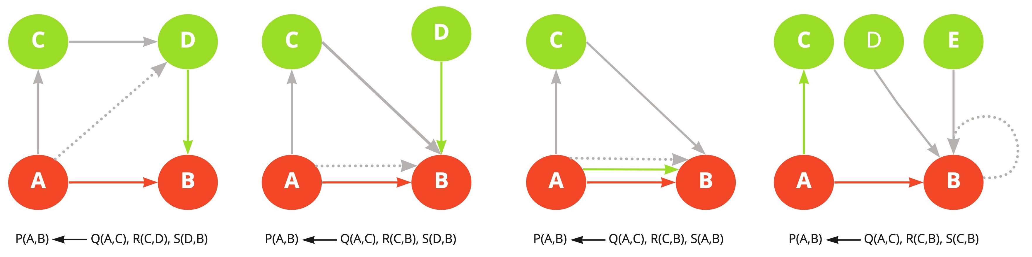
Figure 3: Reduction of Meta-rules with 3 body atoms

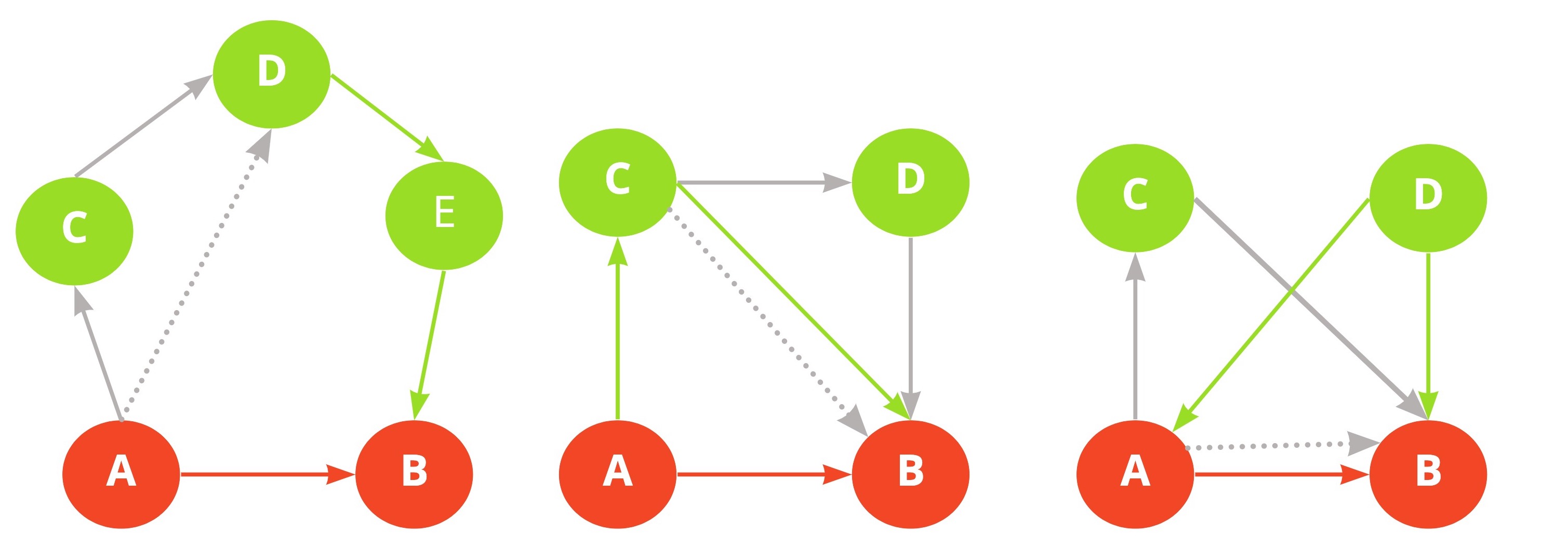
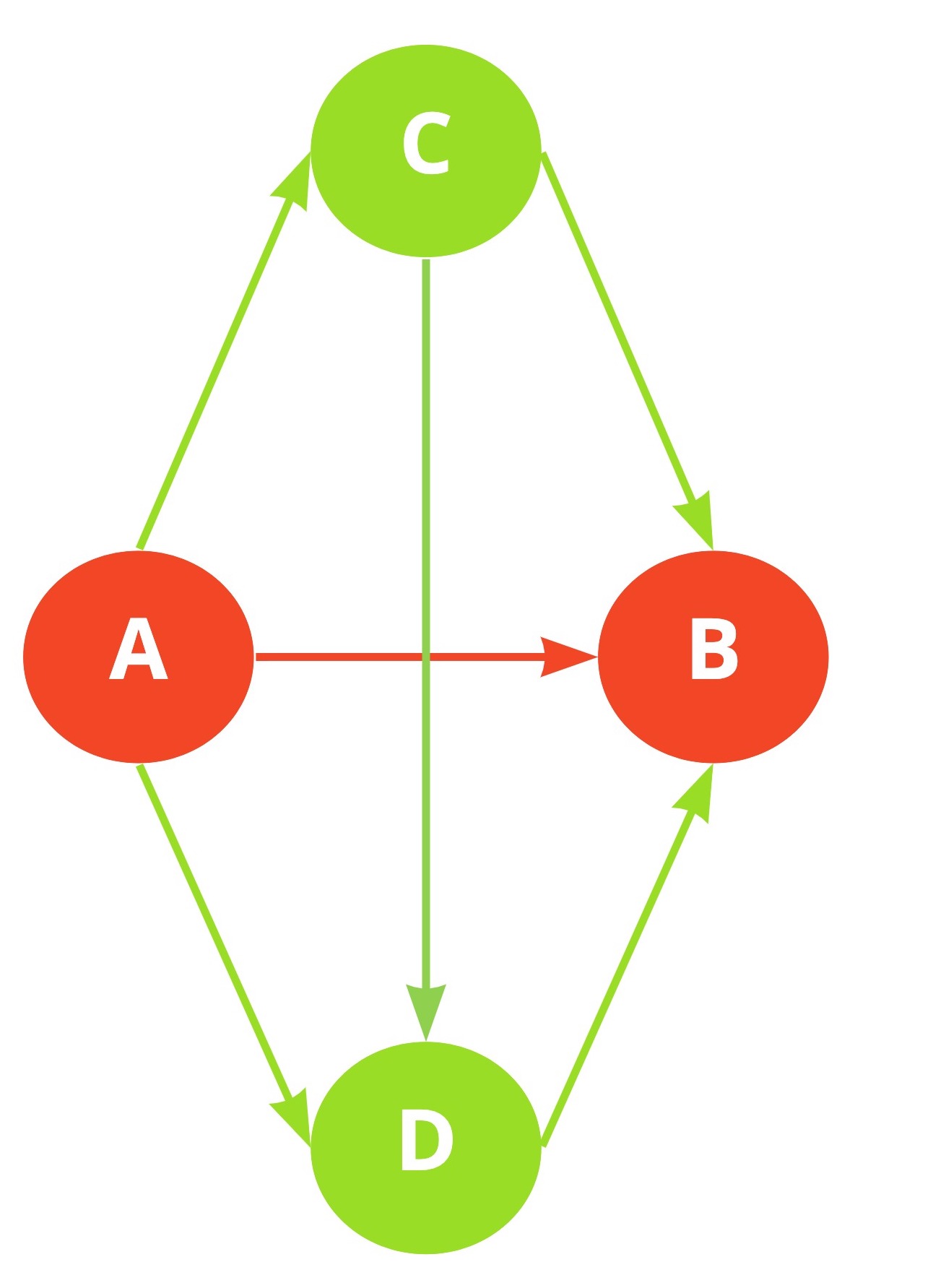
Figure 4: Reduction of Meta-rules with 4 body atoms

Figure 5: Irreducible Meta-Rule with 5 body atoms

Further comparative experiments could be led in the future, to test different minimal or small meta-rules or proto-rules set, and investigate some judicious balance of minimalism/redundancy and expressivity/efficiency in diverse tasks.

Promises

In contrast to most of previous ILP or differentiable ILP works, we hypothesize that our model could be particularly suited for continual learning in semantically-richer domains; for instance, in RL scenarios where an interpretable logic-oriented higher level policy seems pertinent (e.g., autonomous driving). Here some arguments to support this belief:

• In contrast to previous works, our model is independent of the number of predicates, which may vary between training and testing.

• As our experiments in Visual Genome suggest, our model can be boostrapped by semantic or visual priors, to initialise the predicates.

• In semantically-rich domains, the complexity of our model would be more advantageous than other ILP works. Semantically rich domains are characterized by a high number of initial predicates, while enabling a much lower embedding dimension $d$ (as these predicates are highly interdependent), $d<<\mid\mathcal{P}_{0}\mid$; such inequality implies a lower complexity for our model than common methods which have to learn one coefficient per predicate.

• The embedding-based approach enables to reason by analogy, and possibly quickly generalise to new predicates. For instance, if the model has learned the rule $OverTake()\leftarrow\lnot(P(X)\land OnNextLane(X))$, and the embedding $\theta_{P}$ is learned close to $\theta_{Car}$, the rule would generalise to include Truck, assuming $\theta_{Car}\sim\theta_{Truck}$, despite having never seen the new predicate Truck during training.

References

- roc (2017) End-to-end differentiable proving. In Advances in Neural Information Processing Systems 30: Annual Conference on Neural Information Processing Systems 2017, December 4-9, 2017, Long Beach, CA, USA, pages 3788–3800, 2017. URL https://proceedings.neurips.cc/paper/2017/hash/b2ab001909a8a6f04b51920306046ce5-Abstract.html.
- Bordes et al. (2013) A. Bordes, N. Usunier, A. Garcia-Duran, J. Weston, and O. Yakhnenko. Translating embeddings for modeling multi-relational data. In NeurIPS, 2013.
- Campero et al. (2018) A. Campero, A. Pareja, T. Klinger, J. Tenenbaum, and S. Riedel. Logical rule induction and theory learning using neural theorem proving. arXiv preprint arXiv:1809.02193, 2018.
- Cropper and Dumančić (2021) A. Cropper and S. Dumančić. Inductive logic programming at 30: a new introduction. Machine Learning, 43, 2021. ISSN 1573-0565. doi: 10.1007/s10994-021-06089-1. URL https://doi.org/10.1007/s10994-021-06089-1.
- Cropper and Muggleton (2014) A. Cropper and S. Muggleton. Logical minimisation of meta-rules within meta-interpretive learning. In Inductive Logic Programming - 24th International Conference, ILP 2014, volume 9046 of Lecture Notes in Computer Science, pages 62–75. Springer, 2014. doi: 10.1007/978-3-319-23708-4˙5.
- Cropper and Tourret (2018) A. Cropper and S. Tourret. Derivation reduction of metarules in meta-interpretive learning. In ILP, pages 1–21, 01 2018. ISBN 978-3-319-99959-3. doi: 10.1007/978-3-319-99960-9˙1.
- Cropper and Tourret (2020) A. Cropper and S. Tourret. Logical reduction of metarules. 109(7):1323–1369, 2020. doi: 10.1007/s10994-019-05834-x.
- Dai et al. (2019) W.-Z. Dai, Q. Xu, Y. Yu, and Z.-H. Zhou. Bridging machine learning and logical reasoning by abductive learning. In Advances in Neural Information Processing Systems 32, pages 2815–2826. 2019. URL http://papers.nips.cc/paper/8548-bridging-machine-learning-and-logical-reasoning-by-abductive-learning.pdf.
- d’Avila Garcez and Lamb (2020) A. d’Avila Garcez and L. C. Lamb. Neurosymbolic ai: The 3rd wave, 2020.
- Donadello et al. (2017) I. Donadello, L. Serafini, and A. D’Avila Garcez. Logic tensor networks for semantic image interpretation. In International Joint Conference on Artificial Intelligence, pages 1596–1602, 2017. ISBN 978-0-9992411-0-3. doi: 10.24963/InternationalJointConferenceonArtificialIntelligence.2017/221.
- Dong et al. (2019) H. Dong, J. Mao, T. Lin, C. Wang, L. Li, and D. Zhou. Neural Logic Machines. arXiv:1904.11694 [cs, stat], Apr. 2019. arXiv: 1904.11694.
- Evans and Grefenstette (2018) R. Evans and E. Grefenstette. Learning explanatory rules from noisy data. Journal of AI Research, 2018.
- Fonseca et al. (2004) N. Fonseca, V. Costa, F. Silva, and R. Camacho. On avoiding redundancy in inductive logic programming. volume 3194, pages 132–146, 09 2004. ISBN 978-3-540-22941-4. doi: 10.1007/978-3-540-30109-7˙13.
- Galárraga et al. (2013) L. A. Galárraga, C. Teflioudi, K. Hose, and F. Suchanek. AMIE: association rule mining under incomplete evidence in ontological knowledge bases. In Proceedings of the 22nd international conference on World Wide Web, pages 413–422, Rio de Janeiro, Brazil, 2013. ACM Press. ISBN 978-1-4503-2035-1. doi: 10.1145/2488388.2488425.
- Guu et al. (2015) K. Guu, J. Miller, and P. Liang. Traversing knowledge graphs in vector space. In EMNLP, 2015.
- Hudson and Manning (2019a) D. A. Hudson and C. D. Manning. Gqa: A new dataset for real-world visual reasoning and compositional question answering. 2019 IEEE/CVF Conference on Computer Vision and Pattern Recognition (CVPR), pages 6693–6702, 2019a.
- Hudson and Manning (2019b) D. A. Hudson and C. D. Manning. Gqa: A new dataset for real-world visual reasoning and compositional question answering. In CVPR, 2019b.
- Jang et al. (2017) E. Jang, S. Gu, and B. Poole. Categorical reparameterization with gumbel-softmax. In International Conference on Learning Representations, 2017.
- Jiang and Luo (2019) Z. Jiang and S. Luo. Neural Logic Reinforcement Learning. In International Conference on Machine Learning, Apr. 2019.
- Krishna et al. (2017) R. Krishna, Y. Zhu, O. Groth, J. Johnson, K. Hata, J. Kravitz, S. Chen, Y. Kalantidis, L.-J. Li, D. A. Shamma, M. S. Bernstein, and L. Fei-Fei. Visual genome: Connecting language and vision using crowdsourced dense image annotations. Int. J. Comput. Vision, 123(1):32–73, May 2017. ISSN 0920-5691. doi: 10.1007/s11263-016-0981-7.
- Krizhevsky et al. (2017) A. Krizhevsky, I. Sutskever, and G. E. Hinton. Imagenet classification with deep convolutional neural networks. Commun. ACM, 60(6):84–90, May 2017. ISSN 0001-0782. doi: 10.1145/3065386. URL https://doi.org/10.1145/3065386.
- Lin et al. (2015) Y. Lin, Z. Liu, M. Sun, Y. Liu, and X. Zhu. Learning entity and relation embeddings for knowledge graph completion. In In Proceedings of AAAI’15, 2015.
- Maddison et al. (2017) C. J. Maddison, A. Mnih, and Y. W. Teh. The concrete distribution: A continuous relaxation of discrete random variables. In ICLR, 2017. URL https://openreview.net/forum?id=S1jE5L5gl.
- Manhaeve et al. (2018) R. Manhaeve, S. Dumančić, A. Kimmig, T. Demeester, and L. De Raedt. Deepproblog: Neural probabilistic logic programming. In Neural Information Processing Systems, 2018.
- Marcus (2018) G. Marcus. Deep learning: A critical appraisal. arXiv: 1801.00631, 2018.
- (26) S. Muggleton. Inverse entailment and progol. New Generation Computing, 13:245–286.
- Muggleton (1995) S. Muggleton. Inverse entailment and progol, 1995. URL https://doi.org/10.1007/BF03037227.
- Nickel et al. (2011) M. Nickel, V. Tresp, and H.-P. Kriegel. A three-way model for collective learning on multi-relational data. In ICML, 2011.
- Omran et al. (2018) P. Omran, K. Wang, and Z. Wang. Scalable rule learning via learning representation. pages 2149–2155, 07 2018. doi: 10.24963/ijcai.2018/297.
- Payani and Fekri (2019) A. Payani and F. Fekri. Learning algorithms via neural logic networks. arXiv:1904.01554, 2019.
- Quinlan (1990) J. R. Quinlan. Learning logical definitions from relations. MACHINE LEARNING, 5:239–266, 1990.
- Radford et al. (2019) A. Radford, J. Wu, R. Child, D. Luan, D. Amodei, and I. Sutskever. Language models are unsupervised multitask learners. 2019.
- Robinson (1965) J. A. Robinson. A machine-oriented logic based on the resolution principle. J. ACM, 12(1):23–41, Jan. 1965. ISSN 0004-5411. doi: 10.1145/321250.321253. URL https://doi.org/10.1145/321250.321253.
- Santoro et al. (2017) A. Santoro, D. Raposo, D. G. T. Barrett, M. Malinowski, R. Pascanu, P. Battaglia, and T. Lillicrap. A simple neural network module for relational reasoning. 2017.
- Schulman et al. (2017) J. Schulman, F. Wolski, P. Dhariwal, A. Radford, and O. Klimov. Proximal Policy Optimization Algorithms. arXiv preprint: 1707.06347, Aug. 2017.
- (36) R. Socher, D. Chen, C. D. Manning, and A. Y. Ng. Reasoning with neural tensor networks for knowledge base completion.
- Yang et al. (2017) F. Yang, Z. Yang, and W. W. Cohen. Differentiable learning of logical rules for knowledge base reasoning. In Neural Information Processing Systems, 2017.
- Yang and Song (2020) Y. Yang and L. Song. Learn to explain efficiently via neural logic inductive learning. In International Conference on Learning Representations, 2020.
- Zellers et al. (2018) R. Zellers, M. Yatskar, S. Thomson, and Y. Choi. Neural motifs: Scene graph parsing with global context. In CVPR, 2018. URL http://arxiv.org/abs/1711.06640.
- Zimmer et al. (2021) M. Zimmer, X. Feng, C. Glanois, Z. Jiang, J. Zhang, P. Weng, L. Dong, H. Jianye, and L. Wulong. Differentiable logic machines. arXiv preprint arXiv:2102.11529, 2021.