Long Story Short: Omitted Variable Bias in Causal Machine Learning

Abstract.

We derive general bounds on the size of omitted variable bias for a broad class of common causal parameters, such as (weighted) average of potential outcomes, average treatment effects (including subgroup effects, such as the effect on the treated), average causal derivatives, and policy effects from shifts in covariate distribution—all for general, semiparametric and fully nonparametric regression models. Leveraging the Riesz-Frechet representation of the target parameter, we show that the bounds on the bias depend only on the additional variation that latent variables create both in the outcome regression and in the Riesz representer of the causal parameter of interest. We further show how simple plausibility judgments on the maximum explanatory power of latent variables are sufficient to place overall bounds on the size of the bias. Finally, to take the bounds to data, we develop flexible and efficient statistical inference methods on the learnable components of the bounds, which can make use of modern machine learning algorithms for estimation. These results allow empirical researchers to perform sensitivity analyses in a flexible class of machine-learned causal models using very simple, and interpretable, tools. We demonstrate the usefulness of the approach with two empirical examples.

Keywords: sensitivity analysis, short regression, long regression, omitted variable bias, omitted confounders, causal models, machine learning, confidence bounds.

1. Introduction

Causal inference with observational data usually relies on the assumption that the treatment assignment mechanism is “ignorable” (i.e, independent of potential outcomes) conditional on a set of observed variables; or, equivalently, that the set of observed covariates satisfy the “backdoor” (or, more generally, adjustment) criterion (Rosenbaum and Rubin, 1983a; Pearl, 2009; Angrist and Pischke, 2009; Shpitser et al., 2012; Imbens and Rubin, 2015). Investigators who rely on the conditional ignorability assumption for drawing causal inferences from non-experimental studies must, therefore, also be able to cogently argue that there are no unobserved confounders of the treatment-outcome relationship. Yet, claiming the absence of unmeasured confounders is not only fundamentally unverifiable from the data, but often an assumption that is very hard to defend in practice.

When the assumption of no unobserved confounders is called into question, researchers are advised to perform sensitivity analyses, consisting of a formal and systematic assessment of the robustness of their findings against plausible violations of unconfoundedness. The problem of sensitivity analysis has been studied across several disciplines, dating back to, at least, the classical work of Cornfield et al. (1959), and with more recent works from Rosenbaum and Rubin (1983b); Rosenbaum (1987); Robins (1999); Frank (2000); Rosenbaum (2002); Imbens (2003); Brumback et al. (2004); Altonji et al. (2005); Hosman et al. (2010); Imai et al. (2010); Vanderweele and Arah (2011); Blackwell (2013); Frank et al. (2013); Dorie et al. (2016); Oster (2017); VanderWeele and Ding (2017); Yadlowsky et al. (2018); Masten and Poirier (2018); Kallus and Zhou (2018); Kallus et al. (2019); Cinelli et al. (2019); Zhao et al. (2019); Franks et al. (2020); Cinelli and Hazlett (2020a, b); Bonvini and Kennedy (2021); Scharfstein et al. (2021); Jesson et al. (2021), among others. Most of this work, however, either focus exclusively on binary treatments, target a specific estimand of interest (e.g, a causal risk-ratio), or impose parametric assumptions on the observed data, or on the nature of unobserved confounding (see Section 6.1 for further discussion and comparisons, after we present our main results).

In this paper, we derive general, yet simple, sharp bounds on the size of the omitted variable bias for a broad class of causal parameters that can be identified as linear functionals of the conditional expectation function of the outcome. Such functionals encompass many of the traditional targets of investigation in causal inference studies, such as, for example, (weighted) average of potential outcomes, average treatment effects (including subgroup effects, such as the effect on the treated), (weighted) average derivatives, policy effects from shifts in covariate distribution, and others—all for general, nonparametric causal models. Our construction relies on the Riesz-Frechet representation of the target functional. Specifically, we show how the bound on the bias has a simple characterization, depending only on the additional variation that the latent variables create both in the outcome and in the Riesz representer (RR) for the parameter of interest. We can thus perform sensitivity analysis with respect to violations of conditional ignorability in a broad class of causal models and target estimands.

In many leading examples, the Riesz representer in fact corresponds to quantities that are well-known to empirical researchers. For instance, when estimating the average treatment effect in a partially linear model, the RR is the (scaled) residualized treatment, after “partialling out” for control covariates; for the average treatment effect in a general nonparametric model, with a binary treatment, the RR is given by the inverse probability of treatment weights. In such cases, we show how the bounds on the bias can be reparameterized in terms of familiar and interpretable quantities measuring the percentage gains in variance explained (or gains in precision), with the treatment and the outcome, due to confounders. Therefore, plausibility judgments on the maximum explanatory power of latent variables (in predicting the treatment and the outcome) are sufficient to place overall bounds on the bias, simplifying the task of sensitivity analysis even when using nonparametric or otherwise complex models. Similar interpretable quantities arise in other leading examples. We further help analysts place bounds on the size of the bias, by benchmarking the strength of unobserved confounders against the strength of key observed covariates.

Finally we provide flexible statistical inference for these bounds using debiased machine learning (DML) and auto-DML (Chernozhukov et al., 2018a, b, 2020, 2022c). DML methods can be seen as implementing the classical “one-step” semi-parametric correction (Levit, 1975; Hasminskii and Ibragimov, 1978; Pfanzagl and Wefelmeyer, 1985; Bickel et al., 1993) based on regression scores (Newey, 1994) and a Neyman orthogonal score that we obtain for the second moment of the RR, combined with cross-fitting, an efficient form of data-splitting. Our construction makes it possible to use modern machine learning methods for estimating the identifiable components of the bounds, including regression functions, Riesz representers, the norm of regression residuals, and the norm of RRs. Auto-DML further automates the process and estimates RRs using their variational or adversarial characterization, without needing to know their analytical form. We note targeted maximum likelihood estimation (TMLE) methods (Van der Laan and Rose, 2011) could also potentially be employed, though we do not do so here.

In what follows, Section 2 presents our method in the simpler context of partially linear models. The results in that section serve not only as an accessible introduction to the main ideas of our general framework, but are also important in their own right, since partially linear models are widely used in applied work. Section 3 develops the main results of the paper—sharp bounds on the omitted variable bias for continuous linear functionals of the conditional expectation function of the outcome, based on their Riesz representations, all for general, nonparametric causal models. Moreover, the section also provides theoretical details for many important leading examples. In Section 4 we construct high-quality inference methods for the bounds on the target parameters by leveraging recent advances in debiased machine learning with Riesz representers. Section 5 demonstrates the use of our tools to assess the robustness of causal claims in two empirical examples: (i) the impact of 401(k) eligibility on financial assets; and, (ii) the average price elasticity of gasoline demand. Section 6 concludes with a brief discussion of related work, and suggestions for possible extensions.

Notation. All random vectors are defined on the probability space with probability measure ${\mathrm{P}}$. We consider a random vector $Z=(Y,W)$ with distribution $P$ taking values $z$ in its support $\mathcal{Z}$; we use $P_{V}$ to denote the probability law of any subvector $V$ and $\mathcal{V}$ denote its support. We use $\|f\|_{P,q}=\|f(Z)\|_{P,q}$ to denote the $L^{q}(P)$ norm of a measurable function $f:\mathcal{Z}\to\mathbb{R}$ and also the $L^{q}(P)$ norm of random variable $f(Z)$. For a differentiable map $x\mapsto g(x)$, from $\mathbb{R}^{d}$ to $\mathbb{R}^{k}$, $\partial_{x^{\prime}}g$ abbreviates the partial derivatives $(\partial/\partial x^{\prime})g(x)$, and $\partial_{x^{\prime}}g(x_{0})$ means $\partial_{x^{\prime}}g(x)\mid_{x=x_{0}}$. We use $x^{\prime}$ to denote the transpose of a column vector $x$; we use $R^{2}_{U\sim V}$ to denote the $R^{2}$ from the orthogonal linear projection of a scalar random variable $U$ on a random vector $V$. We use the conventional notation $dL/dP$ to denote the Radon-Nykodym derivative of measure $L$ with respect to $P$.

2. Warm-Up: Omitted Variable Bias in Partially Linear Models

To fix ideas, we begin our discussion in the context of partially linear models (PLM). These results not only provide the key intuitions and the building blocks for the general case of nonseparable, nonparametric models of Section 3, but they are also important in their own right, as these models are widely used in applied work.

2.1. Problem set-up

Consider the partially linear regression model of the form

$$Y=\theta D+f(X,A)+\epsilon.$$ (1)

Here $Y$ denotes a real-valued outcome, $D$ a real-valued treatment, $X$ an observed vector of covariates, and $A$ an unobserved vector of covariates. We refer to $W:=(D,X,A)$ as the “long” list of regressors, and to equation (1) as the “long” regression. For now, we assume the error term $\epsilon$ obeys ${\mathrm{E}}[\epsilon|D,X,A]=0$ and thus ${\mathrm{E}}[Y|D,X,A]=\theta D+f(X,A)$.

Under the traditional assumption of conditional ignorability, we have that the regression coefficient $\theta$ identifies the average treatment effect of a unit increase of $D$ on the outcome $Y$, that is,

$${\mathrm{E}}[Y(d+1)-Y(d)]={\mathrm{E}}[{\mathrm{E}}[Y|D=d+1,X,A]-{\mathrm{E}}[Y|D=d,X,A]]=\theta,$$

where $Y(d)$ denotes the potential outcome of $Y$ when the treatment $D$ is experimentally set to $d$. The problem, however, is that $A$ is not observed, and thus both the long regression, and the regression coefficient $\theta$ cannot be computed from the available data.

Since the latent variables $A$ are not measured, an alternative route to obtain an approximate estimate of $\theta$ is to consider the regression of $Y$ on the “short” list of observed regressors $W^{s}:=(D,X)$, as in,

$$Y=\theta_{s}D+f_{s}(X)+\epsilon_{s}.$$ (2)

Following convention, we call equation (2) the “short” regression. Here, again, we assume the error term $\epsilon_{s}$ obeys ${\mathrm{E}}[\epsilon_{s}\mid D,X]=0$ and we thus have ${\mathrm{E}}[Y|D,X]=\theta_{s}D+f_{s}(X)$. We can then use the “short” regression parameter $\theta_{s}$ as a proxy for $\theta$.

Evidently, in general $\theta_{s}$ is not equal to $\theta$, and this naturally leads to the question of how far our “proxy” $\theta_{s}$ can deviate from the true inferential target $\theta$. Our goal is, thus, to analyze the difference between the short and long parameters—the omitted variable bias (OVB):

$$\theta_{s}-\theta,$$

and perform inference on this bias under various hypotheses on the strength of the latent confounders $A$.

2.2. OVB as the covariance of approximation errors

Recall that, using a Frisch-Waugh-Lovell partialling out argument, one can express the long and short regression parameters, $\theta$ and $\theta_{s}$, as the linear projection coefficients of $Y$ on the residuals $D-{\mathrm{E}}[D\mid X,A]$ and $D-{\mathrm{E}}[D\mid X]$, respectively. That is,

$$\theta={\mathrm{E}}Y\alpha(W),\quad\quad\theta^{s}={\mathrm{E}}Y\alpha_{s}(W^{s});$$ (3)

where here we define

$$\alpha(W):=\frac{D-{\mathrm{E}}[D\mid X,A]}{{\mathrm{E}}(D-{\mathrm{E}}[D\mid X,A])^{2}},\quad\alpha_{s}(W^{s}):=\frac{D-{\mathrm{E}}[D\mid X]}{{\mathrm{E}}(D-{\mathrm{E}}[D\mid X])^{2}}.$$

For reasons that will become clear in the next section, we can refer to $\alpha(W)$ and $\alpha_{s}(W^{s})$ as the “long” and “short” Riesz representers (RR).

Now let $g(W):={\mathrm{E}}[Y\mid D,X,A]$ and $g_{s}(W^{s}):={\mathrm{E}}[Y\mid D,X]$ denote the long and short regression functions, respectively. Using the orthogonality conditions in (1) and (2), we can further express $\theta$ and $\theta_{s}$ as

$${\mathrm{E}}Y\alpha(W)={\mathrm{E}}g(W)\alpha(W),\quad\quad{\mathrm{E}}Y\alpha_{s}(W^{s})={\mathrm{E}}g_{s}(W^{s})\alpha_{s}(W^{s}).$$ (4)

Our first characterization of the OVB is thus as follows, where we use the shorthand notation: $g=g(W)$, $g_{s}=g_{s}(W^{s})$, $\alpha=\alpha(W)$, and $\alpha_{s}=\alpha_{s}(W^{s})$.

Theorem 1 (OVB Bounds in PLM).

Assume that $Y$ and $D$ are square integrable with:

$${\mathrm{E}}(D-{\mathrm{E}}[D\mid X,A])^{2}>0.$$

Then the OVB for the partially linear model of equations (1) - (2) is given by

$$\theta_{s}-\theta={\mathrm{E}}(g_{s}-g)(\alpha_{s}-\alpha),$$

that is, it is the covariance between the regression error and the RR error. Furthermore, the squared bias can be bounded as

$$|\theta_{s}-\theta|^{2}=:\rho^{2}B^{2}\leq B^{2},$$

where

$$B^{2}:={\mathrm{E}}(g-g_{s})^{2}{\mathrm{E}}(\alpha-\alpha_{s})^{2},\quad\rho^{2}:=\mathrm{Cor}^{2}(g-g_{s},\alpha-\alpha_{s}).$$

The bound $B^{2}$ is the product of additional variations that omitted confounders generate in the regression function and in the RR. This bound is sharp for the adversarial confounding that maximizes $\rho^{2}$ to $1$ over choices of $\alpha$ and $g$, holding ${\mathrm{E}}(\alpha-\alpha_{s})^{2}$ and ${\mathrm{E}}(g-g_{s})^{2}\leq{\mathrm{E}}(Y-g_{s})^{2}$ fixed.

Note that the bound $B^{2}$ is the maximum amount of squared bias generated by confounding; the actual bias is amortized by the correlation $\rho$, which we call the “degree of adversity.” For a given value of $B$, adversarial confounding would select this correlation to maximize the bias, by setting $\rho^{2}=1$, while amicable confounding would minimize the bias, and set $\rho^{2}=0$. In principle $\rho^{2}$ could be set to various values less than 1 (for example, $\rho^{2}=1/3$) when confounding is assumed to be “natural” rather than adversarial. Here we focus on the maximal degree of adversity, but empirical researchers are free to consider other choices (perhaps motivated by empirical benchmarking; as, for example, in Appendix C).

2.3. Further characterization of the bias

Sensitivity analysis requires making plausibility judgments on the values of the sensitivity parameters. Therefore, it is important that such parameters be well-understood, and easily interpretable in applied settings. Here we show how the bias of Theorem 1 can be further interpreted in terms of conventional $R^{2}$s.

Recall that, when the CEF is not linear, a natural measure of the strength of relationship between some variable $W$ and another variable $V$ is the nonparametric $R^{2}$ (also known as Pearson’s correlation ratio (Pearson, 1905; Doksum and Samarov, 1995)):

$$\eta^{2}_{V\sim W}:=R^{2}_{V\sim{\mathrm{E}}[V|W]}=\operatorname{Var}({\mathrm{E}}[V|W])/\operatorname{Var}(V).$$

Further, the nonparametric partial $R^{2}$ of a variable $V$ with another variable $A$ given variables $D$ and $X$ measures the additional gain in the explanatory power that $A$ provides, beyond what is already is explained by $D$ and $X$:

$$\eta^{2}_{V\sim A\mid DX}:=\frac{\operatorname{Var}({\mathrm{E}}[V|A,D,X])-\operatorname{Var}({\mathrm{E}}[V|D,X])}{\operatorname{Var}(V)-\operatorname{Var}({\mathrm{E}}[V|D,X])}=\frac{\eta^{2}_{V\sim ADX}-\eta^{2}_{V\sim DX}}{1-\eta^{2}_{V\sim DX}}.$$

We are now ready to rewrite the bound of Theorem 1.

Corollary 1 (Interpreting OVB Bounds in Terms of $R^{2}$).

Under the conditions of Theorem 1, we can further express the bound $B^{2}$ as

$$B^{2}=S^{2}C^{2}_{Y}C^{2}_{D},\quad S^{2}:={\mathrm{E}}(Y-g_{s})^{2}{\mathrm{E}}\alpha_{s}^{2},$$ (5)

where

$$\quad C^{2}_{Y}=R^{2}_{Y-g_{s}\sim g-g_{s}}=\eta^{2}_{Y\sim A\mid DX},\quad C^{2}_{D}:=\frac{1-R^{2}_{\alpha\sim\alpha_{s}}}{R^{2}_{\alpha\sim\alpha_{s}}}=\frac{\eta^{2}_{D\sim A\mid X}}{1-\eta^{2}_{D\sim A\mid X}}.$$ (6)

The bound is the product of the term $S^{2}$, which is directly identifiable from the observed distribution of $(Y,D,X)$, and the term $C^{2}_{Y}C^{2}_{D}$, which is not identifiable, and needs to be restricted through hypotheses that limit strength of confounding. The factors $C^{2}_{Y}$ and $C^{2}_{D}$ measure the strength of confounding that the omitted variables generate in the outcome and treatment regressions:

• $\eta^{2}_{Y\sim A\mid DX}$ in the first factor measures the proportion of residual variation of the outcome explained by latent confounders; and,

• $\eta^{2}_{D\sim A\mid X}$ in the second factor measures the proportion of residual variation of the treatment explained by latent confounders.

Note how this result greatly simplifies the complexity of plausibility judgments. No matter how complicated ${\mathrm{E}}[Y|D,X,A]$ and ${\mathrm{E}}[D|X,A]$ are, to place bounds on the size of the bias, researchers need only to reason about the maximum explanatory power that unobserved confounders $A$ have in explaining treatment and outcome variation.

In addition, the corollary also emphasizes a universal OVB formula that holds for general models, and any target parameter that can be expressed as a linear functional of the CEF, which we derive in Section 3. In particular, $C^{2}_{D}$ is determined by $1-R^{2}_{\alpha\sim\alpha_{s}}$—the proportion of residual variation of the long RR generated by latent confounders. In the partially linear model, it turns out that $1-R^{2}_{\alpha\sim\alpha_{s}}$ is simply given by $\eta^{2}_{D\sim A\mid X}$. Similar simplification shows up in many cases, as we will see in Section 3.

Finally, the above results hold for population data. In practice, both $\theta_{s}$ and $S^{2}$ need to be estimated from finite samples. This can be readily done using debiased machine learning, as we discuss in Section 4. This enables efficient statistical inference on the bounds for $\theta$ under any hypothetical strength of the sensitivity parameters $C_{D}$ and $C_{Y}$. These results allow researchers to perform sharp sensitivity analyses in a flexible class of machine-learned causal models using very simple, and interpretable, tools.

2.4. Preview of empirical example.

As a preview of how these bounds can be used in practice, we briefly consider a real example: the robustness of the estimated impact of 401(k) eligibility on financial assets against the presence of unobserved confounders, such as firm characteristics (Poterba et al., 1994, 1995; Chernozhukov et al., 2018a). This example is discussed in detail in Section 5. Here the short regression coefficient is estimated to be $\hat{\theta}_{s}=9051$, suggesting that 401(k) availability leads to an extra $9,051 in financial assets. But how robust is this result to presence of omitted confounders?

Confounding scenarios.

Suppose that latent variables $A$ can explain at most 4% of the residual variation of the outcome, and $3\%$ of the residual variation of the treatment; that is, we have that $\eta^{2}_{Y\sim A\mid DX}=.04$ and $\eta^{2}_{D\sim A\mid X}=.03$. In Section 5 we explain why this may be a conservative scenario. Given the estimate for $\widehat{S}\approx 118K$, these values for the partial $R^{2}$ of $A$ with $Y$ and $D$ translate into an estimated bound on the absolute value of the bias of:

$$|\widehat{B}|=\sqrt{\hat{S}^{2}\left(\frac{\eta^{2}_{Y\sim A\mid DX}\eta^{2}_{D\sim A\mid X}}{1-\eta^{2}_{D\sim A\mid X}}\right)}\approx 4153.$$

In other words, such confounding would lead us to consider a bias of at most $4,153 in our original estimate of $9,051. This implies the following estimated bounds for the target parameter $\theta$ (under maximal confounding with $|\rho|=1$):

$$\widehat{\theta}_{\pm}:=\widehat{\theta}_{s}\pm|\rho||\widehat{B}|\approx 9051\pm 1\cdot 4153=[4898;13204].$$

That is, even under such violation of conditional ignorability, our estimate of the effect of 401(k) availability on financial assets is still large, and it could be anywhere in the stated bounds.

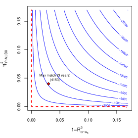
(a) Contours for $|B|$.

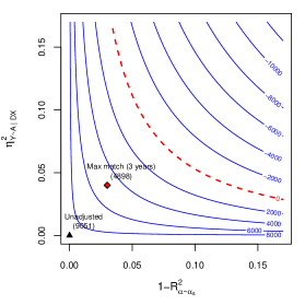
(b) Contours for $\theta_{-}=\theta_{s}-|B|$.

Figure 1. Sensitivity contour plots in the 401(k) example.

Note: The vertical axis shows $\eta^{2}_{Y\sim A\mid DX}$, i.e, the maximum proportion of the residual variation of the outcome that could be explained by latent variables $A$. The horizontal axis shows $1-R^{2}_{\alpha\sim\alpha_{s}}$, i.e, the proportion of variation in the long Riesz Representer which is not explained by the short Riesz Representer. In the partial linear model, this simply equals $\eta^{2}_{D\sim A\mid X}$, i.e, the maximum proportion of the residual variation of the treatment that could be explained by latent variables $A$. Fig. 1(a) shows the contours for the absolute value of the bound on the bias, $|B|$. Fig. 1(b) shows the contours for the lower bound of the target parameter itself, i.e, $\theta_{-}=\theta_{s}-|B|$, which could be brought to the critical value of zero (dashed red contour), or beyond zero.

Sensitivity contours.

A useful tool for visualizing the whole sensitivity range of the target parameter, under different assumptions regarding the strength of confounding, is a bivariate contour plot showing the collection of curves in the space of nonparametric partial $R^{2}$ values ($\eta^{2}_{Y\sim A\mid D,X},\eta^{2}_{D\sim A\mid X}$) along which the bounds are constant. Figure 1 illustrates such curves for the 401(k) example, both for the estimated bound on the absolute value of the bias $|B|$ (Fig 1(a)), and for the estimated lower bound of the target parameter itself, i.e, $\theta_{-}=\theta_{s}-|B|$ (Fig 1(b)). In Fig 1(b), the black triangle in the lower corner shows the original estimate of $9,051. The red diamond shows the lower bound implied by the particular confounding scenario described above, $4,898. But now notice that, with the contour plot, we can readily assess the sensitivity of our estimate to any confounding scenario. In this particular example, for instance, even substantially stronger confounders that explain, say, 10% percent of the residual variation of the treatment and 5% of the residual variation of the outcome (or vice-versa) would not be sufficiently strong to bring down the estimate of the lower bound beyond the critical threshold of zero (although the estimate would be substantially reduced).

All values here were flexibly estimated using Random Forests with debiased machine learning, and we can also account for sampling uncertainty by constructing valid asymptotic confidence intervals for the bounds. Details are provided in Sections 4 and 5.

3. Main Results: Omitted Variable Bias in Nonparametric Causal Models

In this section we derive the main partial identification theorems of the paper, and construct sharp bounds on the size of the omitted variable bias for a broad class of causal parameters that can be identified as linear functionals of the conditional expectation function of the outcome, all for general nonparametric causal models. Although more abstract, the presentation of this section largely parallels the special case of partially linear models given in Section 2.

3.1. Problem set-up

Consider the following modern nonparametric structural equation model (SEM) as an example:

$$Y \leftarrow g_{Y}(D,X,A,\epsilon_{Y}),$$

$$D \leftarrow g_{D}(X,A,\epsilon_{D}),$$

$$A \leftarrow g_{A}(X,\epsilon_{A}),$$

$$X \leftarrow \epsilon_{X},$$

where $Y$ is an outcome variable, $D$ is a treatment variable, $X$ is a vector-valued observed confounder variable, $A$ is a vector-valued latent confounder variable, $\epsilon_{Y},\epsilon_{D},\epsilon_{A}$ are vector-valued structural disturbances that are mutually independent, and $\leftarrow$ denotes assignment. This model has an associated Directed Acyclic Graph (DAG) (Pearl, 2009) as shown in Figure 2.

Figure 2. DAG associated with the SEM.

The SEM above induces the potential outcome $Y(d)$ under the intervention that sets $D$ experimentally to $d$,

$$Y(d):=g_{Y}(d,X,A,\epsilon_{Y}).$$

Additionally, the independence of the structural disturbances implies the following conditional exogeneity (or, ignorability) condition:

$$Y(d)\perp\!\!\!\!\perp D\mid\{X,A\},$$ (7)

which states that the realized treatment $D$ is independent of the potential outcomes, conditionally on $X$ and $A$.

More generally, we can work with any framework that implies potential outcomes $Y(d)$, and such that the conditional exogeneity (7) holds (Imbens and Rubin, 2015). In fact there are many structural causal models that imply potential outcomes and that satisfy the conditional exogeneity assumption (7); (see e.g. Pearl (2009) and Figure 3 for concrete examples). The causal interpretation of our results rely only on the existence of potential outcomes and conditional exogeneity. Under this set-up and when $d$ is in the support of $D$ given $X$, $A$, we then have the following (well-known) identification result

$${\mathrm{E}}[Y(d)\mid X,A]={\mathrm{E}}[Y\mid D=d,X,A]=:g(d,X,A),$$

that is, the conditional average potential outcome coincides with the “long” regression function of $Y$ on $D$, $X$, and $A$. Therefore, we can identify various causal parameters—functionals of the average potential outcome—from the regression function. Important examples include: (i) the average treatment effect (ATE)

$$\theta={\mathrm{E}}[Y(1)-Y(0)]={\mathrm{E}}[g(1,X,A)-g(0,X,A)],$$

for the case of a binary treatment $D$; and, (ii) the average causal derivative (ACD)

$$\theta={\mathrm{E}}\left[\partial_{d}{\mathrm{E}}[Y(D)\mid X,A]\right]={\mathrm{E}}[\partial_{d}g(D,X,A)],$$

for the case of a continuous treatment $D$.

Figure 3. Examples of different DAGs that imply $Y(d)\perp\!\!\!\!\perp D\mid\{X,A\}.$

Note: Examples of DAGs (nonparametric SEMs) that imply the conditional exogeneity condition (7). Latent nodes are circled. In the left DAG, the arrow from $A\to X$ is in reverse order relative to the DAG of Figure 2. In this DAG we still need to condition on $X$ and $A$ to identify the causal effect of $D$ on $Y$. In the center DAG, we need to condition on $A=(A_{1},A_{2})$ and $X$ to identify causal effect of $D$ on $Y$. The center DAG can be viewed as a special case of the left DAG by setting $A=(A_{1},A_{2})$. In the right DAG, it suffices to control for $A$ to identify the average treatment effect of $D$ on $Y$, but we only observe $X_{1}$ and $X_{2}$, the so called “negative” controls, which are measurements, or proxies, of $A$. The conditional exogeneity condition (7) still holds in this case.

In fact, our framework is considerably more general, in that it covers any target parameter of the following general form.

Assumption 1 (Target “Long” Parameter).

The target parameter $\theta$ is a continuous linear functional of the long regression:

$$\theta:={\mathrm{E}}m(W,g);$$ (8)

where the mapping $f\mapsto m(w;f)$ is linear in $f\in L^{2}(P_{W})$, and the mapping $f\mapsto{\mathrm{E}}m(W,f)$ is continuous in $f$ with respect to the $L^{2}(P_{W})$ norm.

This formulation covers the two working examples above with $m(W,g)=g(1,X,A)-g(0,X,A)$ for the ATE and $m(W,g)=\partial_{d}g(D,X,A)$ for the ACD, and the continuity condition holds under the regularity condition provided in the remark below. We discuss many other examples of this form later in Section 3.4.

Remark 1 (Regularity Conditions for ATE and ACD).

As regularity conditions for the ATE we assume ${\mathrm{E}}Y^{2}<\infty$ and the weak overlap condition:

$${\mathrm{E}}[P(D=1\mid X,A)^{-1}P(D=0\mid X,A)^{-1}]<\infty.$$

As regularity conditions for the ACD we assume ${\mathrm{E}}Y^{2}<\infty$, that the conditional density $d\mapsto f(d|x,a)$ is continuously differentiable on its support $\mathcal{D}_{x,a}$, the regression function $d\mapsto g(d,x,a)$ is continuously differentiable on $\mathcal{D}_{x,a}$, and we have that $f(d|x,a)$ vanishes whenever $d$ is on the boundary of $\mathcal{D}_{x,a}$. The above needs to hold for all values $x$ and $a$ in the support of $(X,A)$. We also impose the bounded information assumption:

$${\mathrm{E}}(\partial_{d}\log f(D\mid X,A))^{2}<\infty.$$

These conditions imply that Assumption 1 holds, by Lemma 3 given in Section 3.4. ∎

The key problem is that we do not observe $A$, and therefore we can only identify the “short” conditional expectation of $Y$ given $D$ and $X$, i.e.

$$g_{s}(D,X):={\mathrm{E}}[Y\mid D,X]={\mathrm{E}}[g(D,X,A)|D,X],$$

which, by the tower property, is given by the conditional expectation of the long regression $g(D,X,A)$ given the observed variables $D$ and $X$. With the short regression in hand, we can compute proxies (or approximations) $\theta_{s}$ for $\theta$. In particular, for the ATE, the short parameter consists of

$$\theta_{s}={\mathrm{E}}[g_{s}(1,X)-g_{s}(0,X)],$$

and for the ACD,

$$\theta_{s}={\mathrm{E}}[\partial_{d}g_{s}(D,X)].$$

In this general framework, the proxy parameter can also be expressed as the same linear functional applied to the short regression, $g_{s}(W^{s})$.

Assumption 2 (Proxy “Short” Parameter).

The proxy parameter $\theta_{s}$ is defined by replacing the long regression $g$ with the short regression $g_{s}$ in the definition of the target parameter:

$$\theta_{s}:={\mathrm{E}}m(W,g_{s}).$$

We require $m(W,g_{s})=m(W^{s},g_{s})$, i.e., the score depends only on $W^{s}$ when evaluated at $g_{s}$.

Indeed, in the two working examples this assumption is satisfied, since $m(W,g_{s})=m(W^{s},g_{s})=g_{s}(1,X)-g_{s}(0,X)$ for the ATE and $m(W,g_{s})=m(W^{s},g_{s})=\partial_{d}g_{s}(D,X)$ for the ACD. Section 3.4 verifies this assumption for other examples.

Our goal is to provide bounds on the omitted variable bias (OVB), ie., the difference between the “short” and “long” functionals,

$$\theta_{s}-\theta,$$

under assumptions that limit the strength of confounding, and perform statistical inference on its size.

3.2. Omitted variable bias for linear functionals of the CEF

The key to bounding the bias is the following lemma that characterizes the target parameters and their proxies as inner products of regressions with terms called Riesz representers (RR).

Lemma 1 (Riesz Representation).

There exist unique square integrable random variables $\alpha(W)$ and $\alpha_{s}(W^{s})$, the long and short Riesz representers, such that

$$\theta={\mathrm{E}}m(W,g)={\mathrm{E}}g(W)\alpha(W),\quad\theta_{s}={\mathrm{E}}m(W^{s},g_{s})={\mathrm{E}}g_{s}(W^{s})\alpha_{s}(W^{s}),$$

for all square-integrable $g$’s and $g_{s}$. Furthermore, $\alpha_{s}(W^{s})$ is the projection of $\alpha$ in the sense that

$$\alpha_{s}(W^{s})={\mathrm{E}}[\alpha(W)\mid W^{s}].$$

In the case of the ATE with a binary treatment, the representers are just the classical inverse probability of treatment (Horvitz-Thompson) weights:

$$\alpha(W)=\frac{1(D=1)}{P(D=1\mid X,A)}-\frac{1(D=0)}{P(D=0\mid X,A)},\quad\alpha_{s}(W)=\frac{1(D=1)}{P(D=1\mid X)}-\frac{1(D=0)}{P(D=0\mid X)}.$$

This readily follows from change of measure arguments. While it may not be immediately obvious that $\alpha_{s}=E[\alpha|D,X]$, one can easily show that by applying Bayes’ rule.

In the case of the ACD with a continuous treatment, using integration by parts we can readily verify that the representers are logarithmic derivatives of the conditional densities:

$$\alpha(W)=-\partial_{d}\log f(D\mid X,A),\quad\alpha_{s}(W^{s})=-\partial_{d}\log f(D\mid X).$$

We give more involved examples in the next section.

Sometimes it is useful to impose restrictions on the regression functions, such as partial linearity or additivity. The next lemma describes the RR property for the long and short target parameters in this case.

Lemma 2 (Riesz Representation for Restricted Regression Classes).

Furthermore, if $g$ is known to belong to a closed linear subspace $\Gamma$ of $L^{2}(P_{W})$, and $g_{s}$ is known to belong to a closed linear subspace $\Gamma_{s}=\Gamma\cap L^{2}(P_{W^{s}})$, then there exist unique long RR $\bar{\alpha}$ in $\Gamma$ and unique short RR $\bar{\alpha}_{s}$ in $\Gamma_{s}$ that continue to have the representation property

$$\theta={\mathrm{E}}m(W,g)={\mathrm{E}}g(W)\bar{\alpha}(W),\quad\theta_{s}={\mathrm{E}}m(W^{s},g_{s})={\mathrm{E}}g_{s}(W^{s})\bar{\alpha}_{s}(W^{s}),$$

for all $g\in\Gamma$ and $g_{s}\in\Gamma_{s}$. Moreover, they are given by the orthogonal projections of $\alpha$ and $\alpha_{s}$ on $\Gamma$ and $\Gamma_{s}$, respectively. Since projections reduce the norm, we have ${\mathrm{E}}\bar{\alpha}^{2}\leq{\mathrm{E}}\alpha^{2}$ and ${\mathrm{E}}\bar{\alpha}_{s}^{2}\leq{\mathrm{E}}\alpha_{s}^{2}$. Furthermore, the best linear projection of $\bar{\alpha}$ on $\bar{\alpha}_{s}$ is given by $\bar{\alpha}_{s}$, namely,

$$\min_{b\in\mathbb{R}}{\mathrm{E}}(\bar{\alpha}-b\bar{\alpha}_{s})^{2}={\mathrm{E}}(\bar{\alpha}-\bar{\alpha}_{s})^{2}={\mathrm{E}}\bar{\alpha}^{2}-{\mathrm{E}}\bar{\alpha}^{2}_{s}.$$

In what follows we use the notation $\alpha$ and $\alpha_{s}$ without bars, with the understanding that if such restrictions have been made, then we work with $\bar{\alpha}$ and $\bar{\alpha}_{s}$.

To illustrate, suppose that the regression functions are partially linear, as in Section 2

$$g(W)=\beta D+f(X,A),\\ \quad g_{s}(W^{s})=\beta_{s}D+f_{s}(X),$$

then for either the ATE or the ACD we have that the RR are given by

$$\alpha(W)=\frac{D-{\mathrm{E}}[D\mid X,A]}{{\mathrm{E}}(D-{\mathrm{E}}[D\mid X,A])^{2}},\quad\alpha_{s}(W^{s})=\frac{D-{\mathrm{E}}[D\mid X]}{{\mathrm{E}}(D-{\mathrm{E}}[D\mid X])^{2}}.$$

That is, the representer is given by the (scaled) residualized treatment, which we previously derived using the classical Frisch-Waugh-Lovell theorem, without invoking Riesz representation per se.

Using these lemmas, we immediately obtain the following characterization of the OVB and sharp bounds on its maximal size.

Theorem 2 (OVB and Sharp Bounds).

Consider the long and short parameters $\theta$ and $\theta_{s}$ as given by Assumptions 1 and 2. We then have that the OVB is

$$\theta_{s}-\theta={\mathrm{E}}(g_{s}-g)(\alpha_{s}-\alpha),$$

that is, it is the covariance between the regression error and the RR error. Therefore, the squared bias can be bounded as

$$|\theta_{s}-\theta|^{2}=\rho^{2}B^{2}\leq B^{2},$$

where

$$B^{2}:={\mathrm{E}}(g-g_{s})^{2}{\mathrm{E}}(\alpha-\alpha_{s})^{2},\quad\rho^{2}:=\mathrm{Cor}^{2}(g-g_{s},\alpha-\alpha_{s}).$$

The bound $B^{2}$ is the product of additional variations that omitted confounders generate in the regression function and in the RR. This bound is sharp for the adversarial confounding that maximizes $\rho^{2}$ to $1$ over choices of $\alpha$ and $g$, holding ${\mathrm{E}}(\alpha-\alpha_{s})^{2}$ and ${\mathrm{E}}(g-g_{s})^{2}\leq{\mathrm{E}}(Y-g_{s})^{2}$ fixed.

This is the main conceptual result of the paper, and it is new. It covers a rich variety of causal estimands of interest, as long as they can be written as linear functionals of the long regression. We analyze further examples of this class of estimands in Section 3.4.

Finally, we note the following interesting fact.

Remark 2 (Tighter Bounds under Restrictions).

When we work with restricted parameter spaces, the restricted RRs obey

$${\mathrm{E}}(\bar{\alpha}-\bar{\alpha}_{s})^{2}\leq{\mathrm{E}}(\alpha-\alpha_{s})^{2},$$

since the orthogonal projection on a closed subspace reduces the $L^{2}(P)$ norm. This means that the bounds become tighter in this case. Therefore, by default, when restrictions have been made, we work with restricted RRs. ∎

3.3. Characterization of the OVB bounds

In the same spirit of Section 2, we can further derive useful characterizations of the bounds.

Corollary 2 (Interpreting Bounds).

The bound of Theorem 2 can be re-expressed as

$$B^{2}=S^{2}C^{2}_{Y}C^{2}_{D},\quad S^{2}:={\mathrm{E}}(Y-g_{s})^{2}{\mathrm{E}}\alpha_{s}^{2},$$ (9)

where

$$C^{2}_{Y} := \frac{{\mathrm{E}}(g-g_{s})^{2}}{{\mathrm{E}}(Y-g_{s})^{2}}=R^{2}_{Y-g_{s}\sim g-g_{s}},\quad C^{2}_{D}:=\frac{{\mathrm{E}}\alpha^{2}-{\mathrm{E}}\alpha^{2}_{s}}{{\mathrm{E}}\alpha^{2}_{s}}=\frac{1-R^{2}_{\alpha\sim\alpha_{s}}}{R^{2}_{\alpha\sim\alpha_{s}}}.$$

This generalizes the result of Corollary 1 to fully nonlinear models, and general target parameters defined as linear functionals of the long regression. As before, the bound is the product of the term $S^{2}$, which is directly identifiable from the observed distribution of $(Y,D,X)$, and the term $C^{2}_{Y}C^{2}_{D}$, which is not identifiable, and needs to be restricted through hypotheses that limit strength of confounding.

Thus, again, the terms $C^{2}_{Y}$ and $C^{2}_{D}$ generally measure the strength of confounding that the omitted variables generate in the outcome regression and in the treatment:

• $R^{2}_{Y-g_{s}\sim g-g_{s}}$ in in the first factor measures the proportion of residual variance in the outcome explained by confounders;

• $1-R^{2}_{\alpha\sim\alpha_{s}}$ in the second factor measures the proportion of residual variation of the long RR generated by latent confounders.

Likewise, we have the same useful interpretation of $C^{2}_{Y}$ as the nonparametric partial $R^{2}$ of $A$ with $Y$, given $D$ and $X$, namely, $C^{2}_{Y}=\eta^{2}_{Y\sim A\mid D,X}$. The interpretation of $C^{2}_{D}$ can be further specialized for different cases, as follows.

Remark 3 (Interpretation of $C^{2}_{D}$ for ATE with a Binary Treatment).

For the ATE example, we have that

$$C^{2}_{D}=\frac{{\mathrm{E}}[1/(\pi(X,A)(1-\pi(X,A))]-{\mathrm{E}}[1/(\pi(X)(1-\pi(X))]}{{\mathrm{E}}[1/(\pi(X)(1-\pi(X))]},$$ (10)

where $\pi(X)={\mathrm{P}}(D=1\mid X)$ and $\pi(X,A)={\mathrm{P}}(D=1\mid X,A).$ That is, $C_{D}$ measures the relative gain in predictive power due to $A$ in the treatment model, as measured by the average precision (i.e, the inverse of the variance). Therefore, the interpretation of $C^{2}_{D}$ for the ATE with a binary treatment is similar in spirit to the interpretation for the case of the partially linear model. ∎

And an analogous interpretation applies for average causal derivatives.

Remark 4 (Interpretation of $C_{D}$ for Average Causal Derivatives).

For the ACD example,

$$C^{2}_{D}=\frac{{\mathrm{E}}[(\partial_{d}\log f(D\mid X,A))^{2}]-{\mathrm{E}}[(\partial_{d}\log f(D\mid X))^{2}]}{{\mathrm{E}}[(\partial_{d}\log f(D\mid X))^{2}]},$$ (11)

which can be interpreted as the relative gain in information that the confounder $A$ provides about the location of $D$. If $D$ is homoscedastic Gaussian, conditional on both $X$ and $(X,A)$, we have

$$\partial_{d}\log f(D\mid X,A)=-\frac{D-{\mathrm{E}}[D\mid X,A]}{{\mathrm{E}}(D-{\mathrm{E}}[D\mid X,A])^{2}},\quad\partial_{d}\log f(D\mid X,A)=-\frac{D-{\mathrm{E}}[D\mid X]}{{\mathrm{E}}(D-{\mathrm{E}}[D\mid X])^{2}},$$

so that $C^{2}_{D}$ simplifies to the term $C^{2}_{D}$ found for the partially linear model. ∎

Beyond making direct plausibility judgments on the strength of confounding using the above quantities, analysts can also leverage judgments of relative importance of variables to bound the size of the bias. For instance, if one has reasons to believe that $A$ would not generate as much gains in explanatory power as certain key observed covariates $X_{j}$, this can be used to formally place bounds on the maximal strength of confounding due to $A$. This allows one to assess, for instance, whether confounders as strong or stronger then observed covariates would be sufficient to overturn an empirical result. We elaborate the benchmarking procedure formally in Appendix C and illustrate its use in the empirical application. These results extend previous benchmarking ideas for linear regression models (e.g, Oster, 2017; Cinelli and Hazlett, 2020a) to the general case.

3.4. Theoretical details for leading examples

We now provide theoretical details for a wide variety of interesting and important causal estimands. Recall that we use $W=(D,X,A)$ to denote the “long” set of regressors and $W^{s}=(D,X)$ to denote the “short” list of regressors.

Let us start with examples for the binary treatment case, with the understanding that finitely discrete treatments can be analyzed similarly.

Example 1 (Weighted Average Potential Outcome).

Let $D\in\{0,1\}$ be the indicator of the receipt of the treatment. Define the long parameter as

$$\theta={\mathrm{E}}[g(\bar{d},X,A)\ell(W^{s})],$$

where $w^{s}\mapsto\ell(w^{s})$ is a bounded nonnegative weighting function and $\bar{d}$ is a fixed value in $\{0,1\}$. We define the short parameter as

$$\theta_{s}={\mathrm{E}}[g_{s}(\bar{d},X)\ell(W^{s})].$$

We assume ${\mathrm{E}}Y^{2}<\infty$ and the weak overlap condition

$${\mathrm{E}}[\ell^{2}(W^{s})/P(D=\bar{d}\mid X,A)]<\infty.$$

The long parameter is a weighted average potential outcome (PO) when we set the treatment to $\bar{d}$, under the standard conditional exogeneity assumption (7). The short parameter is a statistical approximation based on the short regression. In this example, setting

• $\ell(w^{s})=1$ gives the average PO in the entire population;

• $\ell(w^{s})=1(x\in{\mathcal{N}})/P(X\in\mathcal{N})$ the average PO for group $\mathcal{N}$;

• $\ell(w^{s})=1(d=1)/P(D=1)$ the average PO for the treated.

Above we can consider $\mathcal{N}$ as small regions shrinking in volume with the sample size, to make the averages local, as in Chernozhukov et al. (2018b), but for simplicity we take them as fixed in this paper.

Example 2 (Weighted Average Treatment Effects).

In the setting of the previous example, define the long parameter

$$\theta={\mathrm{E}}[(g(1,X,A)-g(0,X,A))\ell(W^{s})],$$

and the short parameter as

$$\theta_{s}={\mathrm{E}}[(g_{s}(1,X)-g_{s}(0,X))\ell(W^{s})].$$

We further assume ${\mathrm{E}}Y^{2}<\infty$ and the weak overlap condition

$${\mathrm{E}}[\ell^{2}(W^{s})/\{P(D=0\mid X,A)P(D=1\mid X,A)\}]<\infty.$$

The long parameter is a weighted average treatment effect under the standard conditional exogeneity assumption. In this example, setting

• $\ell(w^{s})=1$ gives ATE in the entire population;

• $\ell(w^{s})=1(x\in\mathcal{N})/P(X\in\mathcal{N})$ the ATE for group $\mathcal{N}$;

• $\ell(w^{s})=1(d=1)/P(D=1)$ the ATE for the treated;

• $\ell(x)=\pi(x)$ the average value of policy (APV) $\pi$,

where the policy $\pi$ assigns a fraction $0\leq\pi(x)\leq 1$ of the subpopulation with observed covariate value $x$ to receive the treatment.

In what follows $D$ does not need to be binary. We next consider a weighted average effect of changing observed covariates $W^{s}$ according to a transport map $w^{s}\mapsto T(w^{s})$, where $T$ is deterministic measurable map from $\mathcal{W}^{s}$ to $\mathcal{W}^{s}$. For example, the policy

$$(D,X,A)\mapsto(D+1,X,A)$$

adds a unit to the treatment $D$, that is $T(W^{s})=(D+1,X)$. This has a causal interpretation if the policy induces the equivariant change in the regression function, namely the counterfactual outcome $\tilde{Y}$ under the policy obeys ${\mathrm{E}}[\tilde{Y}|X,A]=g(T(W^{s}),A)$, and the counterfactual covariates are given by $\tilde{W}=(T(W^{s}),A)$.

Example 3 (Average Policy Effect from Transporting $W^{s}$).

For a bounded weighting function $w^{s}\mapsto\ell(w^{s})$, the long parameter is given by

$$\theta={\mathrm{E}}[\{g(T(W^{s}),A)-g(W^{s},A)\}\ell(W^{s})].$$

The short form of this parameter is

$$\theta_{s}={\mathrm{E}}[\{g_{s}(T(W^{s}))-g_{s}(W^{s})\}\ell(W^{s})].$$

As the regularity conditions we require that the support of $P_{\tilde{W}}=\mathrm{Law}(T(W^{s}),A)$ is included in the support of $P_{W}$, and require the weak overlap condition

$${\mathrm{E}}[(\ell(dP_{\tilde{W}}-dP_{W})/dP_{W})^{2}]<\infty.$$

We now turn to examples with continuous treatments $D$ taking values in $\mathbb{R}^{k}$. Consider the average causal effect of the policy that shifts the distribution of covariates via the map $W=(D,X,A)\mapsto(T(W^{s}),A)=(D+rt(W^{s}),X,A)$ weighted by $\ell(W^{s})$, keeping the long regression function invariant. The following long parameter $\theta$ is an approximation to $1/r$ times this average causal effect for small values of $r$. This example is a differential version of the previous example.

Example 4 (Weighted Average Incremental Effects).

Consider the long parameter taking the form of the average directional derivative:

$$\theta={\mathrm{E}}[\ell(W^{s})t(W^{s})^{\prime}\partial_{d}g(D,X,A)],$$

where $\ell$ is a bounded weighting function and $t$ is a bounded direction function. The short form of this parameter is

$$\theta_{s}={\mathrm{E}}[\ell(W^{s})t(W^{s})^{\prime}\partial_{d}g_{s}(D,X)].$$

As regularity conditions, we suppose that ${\mathrm{E}}Y^{2}<\infty$. Further for each $(x,a)$ in the support of $(X,A)$, and each $d$ in $\mathcal{D}_{x,a}$, the support of $D$ given $(X,A)=(x,a)$, the derivative maps $d\mapsto\partial_{d}g(d,x,a)$ and $d\mapsto g(w)\omega(w)$, for $\omega(w):=\ell(d,x)t(d,x)f(d|x,a)$, are continuously differentiable; the set $\mathcal{D}_{x,a}$ is bounded, and its boundary is piecewise-smooth; and $\omega(w)$ vanishes for each $d$ in this boundary. Moreover, we assume the weak overlap:

$${\mathrm{E}}[(\mathrm{div}_{d}\omega(W)/f(D|X,A))^{2}]<\infty.$$

Another example is that of a policy that shifts the entire distribution of observed covariates, independently of $A$. The following long parameter corresponds to the average causal contrast of two policies that set the distribution of observed covariates $W^{s}$ to $F_{0}$ and $F_{1}$, independently of $A$. Note that this example is different from the transport example, since here the dependence between $A$ and $W^{s}$ is eliminated under the interventions.

Example 5 (Policy Effect from Changing Distribution of $W^{s}$).

Define the long parameter as

$$\theta=\int\left[\int g(w^{s},a)dP_{A}(a)\right]\ell(w^{s})d\mu(w^{s});\quad\mu(w^{s})=F_{1}(w^{s})-F_{0}(w^{s}),$$

where $\ell$ is a bounded weight function, and the short parameter as

$$\theta_{s}=\int g_{s}(w^{s})\ell(w^{s})d\mu(w^{s});\quad\mu(w^{s})=F_{1}(w^{s})-F_{0}(w^{s}).$$

As the regularity conditions we require that the supports of $F_{0}$ and $F_{1}$ are contained in the support of $W^{s}$, and that the measure $dP_{A}\times dF_{k}$ is absolutely continuous with respect to the measure $dP_{W}$ on $\mathcal{A}\times\text{support}(\ell)$. We further assume that ${\mathrm{E}}Y^{2}<\infty$ and the weak overlap:

$${\mathrm{E}}[(\ell[dP_{A}\times d(F_{1}-F_{0})]/dP)^{2}]<\infty.$$

The following result establishes the validity of the OVB formulas and bounds for all examples.

Theorem 3 (OVB Validity in Examples 1-5 ).

Under the conditions stated in Examples 1,2,3,5, Assumptions 1 and 2 are satisfied. Under conditions stated in Example 4, Assumptions 1 and 2 are satisfied for the Hahn-Banach extension of the mapping $g\mapsto{\mathrm{E}}m(W,g)$ to the entire $L^{2}(P_{W})$, given by $g\mapsto{\mathrm{E}}g(W)\alpha(W)$. The m-scores and the corresponding short m-scores in Examples 1-5 are given by:

(1) $m(w,g)=(g(\bar{d},x,a))\ell(w^{s})$; (2) $m(w,g)=(g(1,x,a)-g(0,x,a))\ell(w^{s})$; (3) $m(w,g)=(g(T(w^{s}),a)-g(w^{s},a))\ell(w^{s})$; (4) $m(w,g)=\ell(w^{s})t(w^{s})^{\prime}\partial_{d}g(w)$; (5) $m(w,g)=\int[\int g(w^{s},a)dP_{A}(a)]\ell(w^{s})d\mu(w^{s})$;

(1) $m(w^{s},g_{s})=(g_{s}(\bar{d},x))\ell(w^{s})$; (2) $m(w^{s},g_{s})=(g_{s}(1,x)-g_{s}(0,x))\ell(w^{s})$; (3) $m(w_{s},g)=(g_{s}(T(w^{s}))-g_{s}(w^{s}))\ell(w^{s})$; (4) $m(w^{s},g_{s})=\ell(w^{s})t(w^{s})^{\prime}\partial_{d}g_{s}(w^{s})$; (5) $m(w^{s},g_{s})=\int g_{s}(w^{s})\ell(w^{s})d\mu(w^{s})$.

The long RR and corresponding short RR are given by:

(1) $\alpha(w)=\ \frac{1(d=\bar{d})}{p(\bar{d}\mid x,a)}\bar{\ell}(x,a);$ (2) $\alpha(w)=\ \frac{1(d=1)-1(d=0)}{p(d\mid x,a)}\bar{\ell}(x,a);$ (3) $\alpha(w)=\frac{dP_{\tilde{W}}(w)-dP_{W}(w)}{dP(w)}\ell(w^{s})$; (4) $\alpha(w)=-\frac{\mathrm{div}_{d}(\ell(w^{s})t(w^{s})f(d|x,a))}{f(d|x,a)}$; (5) $\alpha(w)=\ \frac{dP_{A}(a)\times d(F_{1}(w^{s})-F_{0}(w^{s}))}{dP(w)}\ell(w^{s});$

(1) $\alpha_{s}(w^{s})=\ \frac{1(d=\bar{d})}{p(\bar{d}\mid x)}\bar{\ell}(x);$ (2) $\alpha_{s}(w^{s})=\ \frac{1(d=1)-1(d=0)}{p(\bar{d}\mid x)}\bar{\ell}(x);$ (3) $\alpha_{s}(w^{s})=\frac{dP_{\tilde{W}_{s}}(w^{s})-dP_{W^{s}}(w^{s})}{dP_{W^{s}}(w^{s})}\ell(w^{s})$ (4) $\alpha_{s}(w^{s})=-\frac{\mathrm{div}_{d}(\ell(w^{s})t(w^{s})f(d|x))}{f(d|x)}$; (5) $\alpha_{s}(w^{s})=\ \frac{d(F_{1}(w^{s})-F_{0}(w^{s}))}{dP_{W^{s}}(w^{s})}\ell(w^{s});$

where above we used the notations: $\bar{\ell}(X,A):={\mathrm{E}}[\ell(W^{s})|X,A],\bar{\ell}(X):={\mathrm{E}}[\ell(W^{s})|X]$, $p(d\mid x,a):={\mathrm{P}}(D=d|X=x,A=a),p(d\mid x):={\mathrm{P}}(D=d|X=x).$ In Examples 1-2, when the weight function only depends on $X$, namely $\ell(W^{s})=\ell(X)$, we have the simplifications $\bar{\ell}(X,A)=\bar{\ell}(X)=\ell(X).$

4. Statistical Inference on the Bounds

The bounds for the target parameter $\theta$ take the form

$$\theta_{\pm}=\theta_{s}\pm|\rho|SC_{Y}C_{D},\quad S^{2}={\mathrm{E}}(Y-g_{s})^{2}{\mathrm{E}}\alpha^{2}_{s}.$$

The components $C_{Y}$, $C_{D}$ are set through hypotheses on the explanatory power of omitted variables. The correlation (degree of confounding) $|\rho|$ can be set to 1 under adversarial confounding. The unknown components of the bounds are $S$ and $\theta_{s}$. We can estimate these components via debiased machine learning (DML), which is a form of the classical “one-step” semi-parametric correction (Levit, 1975; Hasminskii and Ibragimov, 1978; Pfanzagl and Wefelmeyer, 1985; Bickel et al., 1993; Chernozhukov et al., 2022a) based on regression scores (Newey, 1994) and a Neyman orthogonal score we give for the second moment of the RR, combined with cross-fitting, an efficient form of data-splitting.

For debiased machine learning of $\theta_{s}$, we exploit the representation

$$\theta_{s}={\mathrm{E}}[m(W^{s},g_{s})+(Y-g_{s})\alpha_{s}],$$

as in Chernozhukov et al. (2022c, 2021). This representation is Neyman orthogonal with respect to perturbations of $(g_{s},\alpha_{s})$, which is a key property required for DML. Another component to be estimated is

$${\mathrm{E}}(Y-g_{s})^{2}=:\sigma^{2}_{s},$$

which is also Neyman-orthogonal with respect to $g_{s}$. The final component to be estimated is ${\mathrm{E}}\alpha^{2}_{s}$. For this we explore the following formulation:

$${\mathrm{E}}\alpha^{2}_{s}=2{\mathrm{E}}m(W^{s},\alpha_{s})-{\mathrm{E}}\alpha^{2}_{s}=:\nu^{2}_{s},$$

where the latter parameterization is Neyman-orthogonal. Specifically Neyman orthogonality refers to the property:

$$\partial_{g,\alpha}{\mathrm{E}}[m(W^{s},g)+(Y-g)\alpha]\Big{|}_{\alpha=\alpha_{s},g=g_{s}}=0;$$

$$\partial_{g}{\mathrm{E}}(Y-g)^{2}\Big{|}_{g=g_{s}}=0;$$

$$\partial_{\alpha}{\mathrm{E}}[2m(W^{s},\alpha)-\alpha^{2}]\Big{|}_{\alpha=\alpha_{s}}=0;$$

where $\partial$ is the Gateaux (pathwise derivative) operator over directions $h\in L^{2}(P_{W^{s}})$.

Application of DML theory in Chernozhukov et al. (2018a) and the delta-method gives the statistical properties of the estimated bounds under the condition that machine learning of $g_{s}$ and $\alpha_{s}$ is of sufficiently high quality, with learning rate faster than $n^{-1/4}$.

The estimation relies on the following generic algorithm.

Definition 1 (DML($\psi$)).

Input the Neyman-orthogonal score $\psi(Z;\beta,\eta)$, where $\eta=(g,\alpha)$. Then (1), given a sample $(Z_{i}:=(Y_{i},D_{i},X_{i}))_{i=1}^{n}$, randomly partition the sample into folds $(I_{\ell})_{\ell=1}^{L}$ of approximately equal size. Denote by $I_{\ell}^{c}$ the complement of $I_{\ell}$. (2) For each $\ell$, estimate $\widehat{\eta}_{\ell}=(\widehat{g}_{\ell},\widehat{\alpha}_{\ell})$ from observations in $I_{\ell}^{c}$. (3) Estimate $\beta$ as a root of: $0=n^{-1}\sum_{\ell=1}^{L}\sum_{i\in I_{\ell}}\psi(\beta,Z_{i};\widehat{\eta}_{\ell}).$ Output $\widehat{\beta}$ and the estimated scores $\widehat{\psi}^{o}(Z_{i})=\psi(\widehat{\beta},Z_{i};\widehat{\eta}_{\ell})$ for each $i\in I_{\ell}$ and each $\ell$.

Therefore the estimators are defined as

$$\widehat{\theta}_{s}:=\mathrm{DML}(\psi_{\theta});\quad\widehat{\sigma}^{2}_{s}:=\mathrm{DML}(\psi_{\sigma^{2}});\quad\widehat{\nu}^{2}_{s}:=\mathrm{DML}(\psi_{\nu^{2}});$$

for the scores

$$\psi_{\theta}(Z;\theta,g,\alpha):=m(W^{s},g)+(Y-g(W^{s}))\alpha(W^{s})-\theta;$$

$$\psi_{\sigma^{2}}(Z;\sigma^{2},g):=(Y-g(W^{s}))^{2}-\sigma^{2};$$

$$\psi_{\nu^{2}}(Z;\nu^{2},\alpha):=(2m(W^{s},\alpha)-\alpha^{2})-\nu^{2}.$$

We say that an estimator $\hat{\beta}$ of $\beta$ is asymptotically linear and Gaussian with the centered influence function $\psi^{o}(Z)$ if

$$\sqrt{n}(\hat{\beta}-\beta)=\frac{1}{\sqrt{n}}\sum_{i=1}^{n}\psi^{o}(Z_{i})+o_{{\mathrm{P}}}(1)\leadsto N(0,{\mathrm{E}}\psi^{o2}(Z)).$$

The application of the results in Chernozhukov et al. (2018a) for linear score functions yields the following result.

Lemma 3 (DML for Bound Components).

Suppose that each of $\psi$’s listed above and the machine learners $\hat{\eta}_{\ell}=(\alpha_{\ell},g_{\ell})$ of $\eta_{0}=(g_{s},\alpha_{s})$ in $L^{2}(P_{W^{s}})$ obey Assumptions 3.1 and 3.2 in Chernozhukov et al. (2018a), in particular the rate of learning $\eta_{0}$ in the $L^{2}(P_{W^{s}})$ norm needs to be $o_{P}(n^{-1/4})$. Then the estimators are asymptotically linear and Gaussian with influence functions:

$$\psi^{o}_{\theta}(Z):=\psi_{\theta}(Z;\theta_{s},g_{s},\alpha_{s});\quad\psi^{o}_{\sigma^{2}}(Z):=\psi_{\sigma^{2}}(Z;\sigma^{2}_{s},g_{s});\quad\psi^{o}_{\nu^{2}}(Z):=\psi_{\nu^{2}}(Z;\nu^{2}_{s},\alpha_{s}).$$

The covariance of the scores can be estimated by the empirical analogues using the covariance of the estimated scores.

The resulting plug-in estimator for the bounds is then:

$$\widehat{\theta}_{\pm}=\widehat{\theta}_{s}\pm\widehat{S}|\rho|C_{Y}C_{D},\quad\widehat{S}^{2}=\widehat{\sigma}^{2}_{s}\widehat{\nu}^{2}_{s}.$$

Theorem 4 (DML Confidence Bounds for Bounds).

Under the conditions of Lemma 3, the plug-in estimator $\widehat{\theta}_{\pm}$ is also asymptotically linear and Gaussian with the influence function:

$$\varphi^{o}_{\pm}(Z)=\psi^{o}_{\theta}(Z)\pm\frac{|\rho|}{2}\frac{C_{Y}C_{D}}{S}(\sigma^{2}_{s}\psi^{o}_{\nu^{2}}(Z)+\nu_{s}^{2}\psi^{o}_{\sigma^{2}}(Z)).$$

Therefore, the confidence bound

$$[\ell,u]=\left[\widehat{\theta}_{-}-\Phi^{-1}(1-a)\sqrt{\frac{{\mathrm{E}}\varphi^{o2}_{-}}{n}},\ \widehat{\theta}_{+}+\Phi^{-1}(1-a)\sqrt{\frac{{\mathrm{E}}\varphi^{o2}_{+}}{n}}\right]$$

has the one-sided covering property, namely

$${\mathrm{P}}(\theta_{-}\geq\ell)\to 1-a\text{ and }{\mathrm{P}}(\theta_{+}\leq u)\to 1-a.$$

The same results continue to hold if ${\mathrm{E}}\varphi^{o2}_{\pm}(Z)^{2}$ are replaced by the empirical analogue

$$\frac{1}{n}\sum_{\ell=1}^{L}\sum_{i\in I_{\ell}}\hat{\varphi}^{o2}_{\pm}(Z_{i}).$$

Remark 5 (Confidence Bounds).

The above interval has the following set-wise covering property for the region $[\theta_{-},\theta_{+}]$: the region is covered with probability no less than $1-2a-o(1)$, by the union bound. However, as argued by Imbens and Manski (2004), the goal is often to cover a true value $\theta\in[\theta_{-},\theta_{+}]$ with a prescribed probability, which is a two-sided point-wise covering property. The above confidence interval does cover any such $\theta$ with probability no less than $1-a-o(1)$, when the width of the bound $B$ is bounded away from zero. This follows by the argument of Imbens and Manski (2004). If we want to have the two-sided pointwise covering property to be uniform in $B\approx 0$, then we can use the further adjustment of Stoye (2009) to guarantee that. For simplicity though, we focus on the one-sided covering property stated in the theorem, because in applications the relevant hypotheses are often one-sided.∎

The following remark discusses learning the regression function $g_{s}$ and the Riesz representer $\alpha_{s}$.

Remark 6 (Machine Learning of $\alpha_{s}$ and $g_{s}$).

Estimation of the short regression $g_{s}$ is standard and a variety of modern methods can be used (neural networks, random forests, penalized regressions). Estimation of the short RR $\alpha_{s}$ can proceed in one of the following ways. First, we can use analytical formulas for $\alpha_{s}$ (see e.g., Chernozhukov et al. (2018a); Semenova and Chernozhukov (2021), and references therein, for practical details). Second, we can use a variational characterization of $\alpha_{s}$:

$$\alpha_{s}=\arg\min_{\alpha\in\mathcal{A}}{\mathrm{E}}[\alpha^{2}(W^{s})-2m(W^{s},\alpha)],$$

where $\mathcal{A}$ is the parameter space for $\alpha_{s}$, as proposed in Chernozhukov et al. (2021, 2022c). This avoids inverting propensity scores or conditional densities, as usually required when using analytical formulas. This approach is motivated by the first-order-conditions of the variational characterization:

$${\mathrm{E}}\alpha_{s}g={\mathrm{E}}m(W^{s},g)\quad\text{ for all $g$ in $\mathcal{G}$, }$$

which is the definition of the RR. Neural network (RieszNet) and random forest (ForestRiesz) implementations of this approach are given in Chernozhukov et al. (2022b), and the Lasso implementation in Chernozhukov et al. (2022c). Third, we may use a minimax (adversarial) characterization of $\alpha_{s}$, as in Chernozhukov et al. (2018b, 2020):

$$\alpha_{s}=\arg\min_{\alpha\in\mathcal{A}}\max_{g\in\mathcal{G}}|{\mathrm{E}}m(W^{s},g)-{\mathrm{E}}\alpha g|,$$

where $\mathcal{A}$ is the parameter space for $\alpha_{s}$. The Dantzig selector implementation of this approach is given in Chernozhukov et al. (2018b). The neural network implementation of this approach is given in Chernozhukov et al. (2020).∎

5. Empirical Examples

We now re-analyze two empirical examples: (i) the causal effect of 401(k) eligibility on net financial assets (Poterba et al., 1994, 1995; Chernozhukov et al., 2018a); and, (ii) the price elasticity of gasoline demand (Blundell et al., 2012, 2017; Chetverikov and Wilhelm, 2017). Our goal is to complement previous studies with a sensitivity analysis, utilizing the methods developed in the present paper. More specifically we want to determine whether prior conclusions, reached under the assumption of conditional ignorability, are robust to potential uncontrolled confounding. As a preview of the results, we find that the conclusions of the first example are robust to plausible scenarios of latent confounding, whereas in the second example this is not the case.

5.1. The effect of 401(k) eligibility on financial assets

A 401(k) plan is an employed sponsored tax-deferred savings option that allows individuals to deduct contributions from their taxable income, and accrue tax-free interest on investments within the plan. Introduced in the early 1980s as an incentive to increase individual savings for retirement, an important question in the savings literature is precisely to quantify the causal impact of 401(k) eligibility on net financial assets. Indeed, a naive comparison of net financial assets between those individuals with and without 401(k) eligibility suggests a positive and large impact: using data from the 1991 Survey of Income and Program Participation (SIPP), this difference amounts to $19,559.

The problem of this naive comparison, however, is that 401(k) plans can be obtained only by those individuals that work for a firm that offers such savings option—and employment decisions are far from randomized. As an attempt to overcome this lack of random assignment, Poterba et al. (1994), Poterba et al. (1995), and more recently Chernozhukov et al. (2018a), leveraged the 1991 SIPP data to adjust for potential confounding factors between 401(k) eligibility and the financial assets of an individual. Their main argument is that eligibility for enrolling in a 401(k) plan can be taken as exogenous after conditioning on a few observed variables, most importantly, income. As explained in Poterba et al. (1994), at least around the time 401(k) plans initially became available, people were unlikely to make employment decisions based on whether an employer offered a 401(k) plan; instead, their main focus were on salary and other aspects of the job. Thus, whether one is eligible for a 401(k) plan could be taken as ignorable once we condition on income and other covariates related to job choice.

(a) Ignorability holds conditional on $X$ only.

(b) Ignorability holds conditional on $X$ and $F$.

Figure 4. Two possible causal DAGs for the 401(K) example.

It is useful to think about causal diagrams (Pearl, 2009) that represent this identification strategy. One possible model is shown Figure 4(a). Here our outcome variable, $Y$, consists of net financial assets; the treatment variable, $D$, is an indicator for being eligible to enroll in a 401(k) plan; finally, the vector of observed covariates, $X$, consists of: (i) age; (ii) income; (iii) family size; (iv) years of education; (iv) a binary variable indicating marital status; (v) a “two-earner” status indicator; (vi) an IRA participation indicator; and, (vii) a home ownership indicator. We consider that the decision to work for a firm that offers a 401(k) plan depends both on the observed covariates $X$, but also on latent firm characteristics, denoted by $F$; moreover, $X$, $F,$ and $D$ are jointly affected by a set of latent factors $U$. Most importantly, note the assumption of absence of direct arrows, both from $F$ and $U$, to $Y$. Under such assumption, conditional ignorability holds adjusting for $X$ only. The story represented by the DAG of Figure 4(a) is one way of rationalizing the identification strategy used in earlier papers.

The first two columns of Table 1 shows the estimates for the average treatment effect of 401(k) eligibility on net financial assets under this conditional ignorability assumption. For these estimates, we follow the same strategy used in Chernozhukov et al. (2018a), and we estimate the causal effect using DML with Random Forests, considering both a partially linear model (PLM), and a fully nonparametric model (NPM). As we can see, after flexibly taking into account observed confounding factors, although the estimates of the effect of 401(k) eligibility on net financial assets are substantially attenuated, they are still large, positive and statistically significant (more precisely, $9K for the PLM and $8K for the NPM).

With the nonparametric model, we further explore heterogeneous treatment effects, by analyzing the ATE within income quartile groups. The results are shown in Figure 5(a). We see that the ATE varies substantially across groups, with effects ranging from approximately $5,000 (first quartile) to almost $20,000 (last quartile).

	Short Results				Robustness Values
Model	Short Estimate	Std. Error			$\text{RV}_{\theta=0}$	$\text{RV}_{\theta=0,a=0.05}$
Partially Linear	9,051	1,313			7.4%	5.5%
Fully Nonparametric	8,076	1,164			6.2%	4.7%

Table 1. Minimal sensitivity reporting, 401(k).

Omitted confounder analysis

It is now useful to consider scenarios in which conditional ignorability fails. Figure 4(b) presents one such scenario, where a violation of conditional ignorability is credible. Employers often offer a benefit in which they “match” a proportion of an employee’s contribution to their 401(k) up to 5% of the employee’s salaries. The model in Figure 4(b) allows this “matched amount,” denoted by $M$, to be determined by unobserved firm characteristics $F$, observed worker characteristics $X$, and by 401(k) eligibility $D$. In this model, adjustment for $X$ alone is not sufficient for control of confounding. Instead, we now need to condition both on observed covariates $X$ and latent confounders $F$ for ignorability to hold.

How strong would the omitted firm characteristics $F$ have to be in order to overturn our previous conclusions? How would our estimates have changed under certain posited strengths of the explanatory power of firm characteristics? And how plausible are the strengths revealed to be problematic? In what follows, we use our sensitivity analysis results to address these questions.

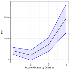
(a) Estimates under no confounding.

(b) Bounds under posited confounding.

Figure 5. One-Sided Confidence Bounds for the ATE by Income Quartiles.

Note: Estimate (black), bounds (red), and confidence bounds (blue) for the ATE. Confounding scenario: $\rho^{2}=1$; $C^{2}_{Y}\approx 0.04$; $C^{2}_{D}\approx 0.031$. Significance level of 5%.

Minimal sensitivity reporting.

In reporting empirical results, the following definitions will be useful.

Definition 2 (Robustness Values).

The robustness $RV_{\theta}$ stands for the minimum bound $RV$ on both sensitivity parameters, $\eta^{2}_{Y\sim F\mid D,X}\leq\text{RV}$ and $1-R^{2}_{\alpha\sim\alpha_{s}}\leq\text{RV}$, such that the interval $[\widehat{\theta}_{-},\widehat{\theta}_{+}]$ of Theorem 4 includes the hypothesis $\theta$ (typically, the zero effect hypothesis $\theta=0$). $\text{RV}_{\theta,a}$ stands for the minimum bound such that the interval $[l,u]$ of Theorem 4 includes $\theta$, at the significance level $a$.

For example, $\text{RV}_{\theta=0}$ measures the minimal equal strength of both confounding factors such that the estimated bound for the ATE would include zero; and $\text{RV}_{\theta=0,a=.05}$ measures the the minimal equal strength of both confounding factors such that the estimated confidence bound for the ATE would include zero, at the 5% significance level.

In Table 1 we report the robustness values of the short estimate, both for the PLM and the fully nonparametric model. Starting with the PLM, the $\text{RV}_{\theta=0}$ of 7.4% means that unobserved confounders that explain less than 7.4% of the residual variation, both of the treatment, and of the outcome, are not sufficiently strong to explain away the observed effect. If we further account for sampling uncertainty (at the 5% significance level), we obtain an $\text{RV}_{\theta=0,a=0.05}$ of 5.5%, meaning that if latent firm characteristics explain less than 5.5% of the residual variation, both of 401(k) eligibility and net financial assets, this would not be sufficient to bring down the lower limit of the confidence bound for the ATE to zero. Moving to the fully nonparametric model, we obtain similar, but somewhat lower values of $\text{RV}_{\theta=0}=6.2\%$ and $\text{RV}_{\theta=0,a=0.05}=4.7\%$. The RV thus provides a quick and meaningful reference point that summarizes the robustness of the short estimate against unobserved confounding—any postulated confounding that does not meet this minimal criterion of strength cannot overturn the results of the original study.

Main confounding scenario.

We now proceed to construct a particular confounding scenario, based on the contextual details of the problem. We start with the assumption that $F$ explains as much variation in net financial assets as the total variation of the maximal matched amount of income (5%) over the period of three years (roughly the period over which the effect is measured) . In the worst case scenario, this would lead to an additional $3\%$ of total variation explained, resulting in a partial $R^{2}$ of outcome with omitted firm characteristics $F$ of $C_{Y}^{2}=\eta^{2}_{Y\sim F|DX}=4\%$. This amounts to a relative increase of approximately 10% in the baseline $R^{2}$ of the outcome regression of 28%. Following similar reasoning, and more conservatively, we posit that omitted firm characteristics can explain an additional $2.5\%$ of the variation in 401(k) eligibility, corresponding to a $22\%$ relative increase in the baseline $R^{2}$ of the treatment regression of 11.4%. For the partially linear model, this results in $1-R^{2}_{\alpha\sim\alpha_{s}}=\eta^{2}_{D\sim F\mid X}\approx 3\%$ (and also $C^{2}_{D}\approx 3\%$).. We adopt the same scenario for the nonparametric model. Since both $\eta^{2}_{Y\sim F|DX}\approx 4\%$ and $1-R^{2}_{\alpha\sim\alpha_{s}}\approx 3\%$ are below the robustness value of 5.5% (or 4.7%) , we immediately conclude that such confounding scenario is not capable of bringing the lower limit of the confidence bound of the ATE to zero.

Model	Short Estimate	|Bias| Bound	ATE Bounds	Confidence Bounds
Partially Linear	9,051 (1,313)	4,153 (307)	[4,898; 13,204]	[2,715 ; 15,458]
Fully Nonparametric	8,076 (1,164)	4,459 (325)	[3,618; 12,535]	[1,654; 14,547]

Note: $\rho^{2}=1$; $C^{2}_{Y}\approx 0.04$; $C^{2}_{D}\approx 0.03$. Significance level of 5%. Standard errors in parenthesis.

Table 2. Estimate, bias, and bounds for the ATE, 401(k).

Next we determine the exact bias, bounds, and confidence bounds on the ATE implied by the posited scenario, as shown in Table 2. Starting with the partially linear model, we see that the confounding scenario would create an estimated absolute bias of at most $\$4,153$. Accounting for statistical uncertainty, we obtain a lower limit for the confidence bound of $\$2,715$. The results for the fully nonparametric model are qualitatively similar, with point estimates and bounds for the ATE shifted down by roughly one thousand dollars. Confidence bounds for group-wise ATEs can also be computed, and are shown in Figure 5(b). Note how the bounds are still largely positive, with only a small excursion into the negative side in the case of the second quartile group. These results suggest that the main qualitative findings reported in earlier studies are robust to the violation of unconfoundedness specified by the confounding scenario above.

Benchmarking against observed covariates.

Another approach to construct confounding scenarios is to use observed covariates to “benchmark” the plausible strength of unobserved covariates. Here we consider the variables (i) income, (ii) whether a worker has an individual retirement account, and (iii) whether the worker’s family has a two-earner status. These observed covariates were chosen because of their financial nature, and they may be acting similarly to the effect of omitted firm characteristics via match amount. As shown in Appendix C, apart from income, all these covariates have limited estimated explanatory power, and result in weaker confounding scenarios than the one we have previously considered. We conclude that, for latent confounders to completely eliminate the observed effect, they would need to generate higher gains in explanatory power than the gains generated by key observed covariates.

Sensitivity contour plots.

Contour plots for the absolute value of the bias, as well as for the estimated lower bound of the ATE, were already given in Figure 1 of Section 2.4. Here we provide analogous plots for the lower limit and upper limit of the confidence bounds for the ATE. These plots allow investigators to quickly and easily assess the robustness of their findings against any postulated confounding scenario.

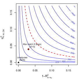
(a) Contours lower limit confidence bound (PLM).

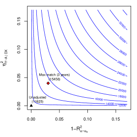
(b) Contours upper limit confidence bound (PLM).

Figure 6. Sensitivity contour plots 401(k), PLM. Significance level $a=0.05$.

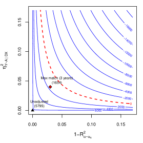
(a) Contours lower limit confidence bound (NPM).

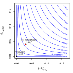
(b) Contours upper limit confidence bound (NPM).

Figure 7. Sensitivity contours 401(k), NPM. Significance level $a=0.05$.

Starting with the partially linear model, the results are shown in Figure 6. As before, the horizontal axis describes the fraction of residual variation of the treatment explained by unobserved confounders, whereas the vertical axis describes the share of residual variation of the outcome explained by unobserved confounders. The contour lines show the lower limit (Figure 6(a)) and upper limit (Figure 6(b)) of the confidence bounds $[l,u]$ for the ATE (see Theorem 4), with a given pair of hypothesized values of partial $R^{2}$ (and the conservative assumption of adversarial confounding, $\rho=1$). Note $\text{RV}_{\theta=0,a=0.05}$ of Table 1 is the point where the 45-degree line crosses the critical contour of zero (red dashed line), offering a convenient and interpretable summary of the critical contour.

We can further place reference points on the contour plots, indicating plausible bounds on the strength of confounding, under alternative assumptions about the maximum explanatory power of omitted variables. The red diamond point on the plot—Max match (3 years)—shows the bounds on the partial $R^{2}$ as previously discussed, resulting in confidence bounds for the ATE of $2,715 to $15,458, in accordance with Table 2. Note here we consider adversarial confounding, by setting $\rho=1$. Setting $\rho$ to a value similar to what is observed for income results in a much weaker scenario (see Appendix C for details). Contour plots for the nonparametric model are very similar, and are provided in Figure 7.

5.2. Average price elasticity of gasoline demand

An important part of estimating the welfare consequences of price changes is to identify the price elasticity of demand. Here we re-analyze the data on gasoline demand from the 2001 National Household Travel Survey (NHTS) (Blundell et al., 2012, 2017; Chetverikov and Wilhelm, 2017). This is a household level survey conducted by telephone and complemented by travel diaries and odometer readings (see Blundell et al. (2012) and ORNL (2004) for details). Important variables in the survey include household income, gasoline price, and annual gasoline consumption (as inferred by odometer readings and fuel efficiency of vehicles). Income data corresponds to the median of the income bracket of the household, with $15$ income brackets equally spaced apart in the logarithmic scale. The survey also contains $24$ covariates related to population density, urbanization, demographics and US Census region indicators.

	Short Results			Robustness Values
Model	Short Estimate	Std. Error		$\text{RV}_{\theta=-1.5}$	$\text{RV}_{\theta=-1.5,a=0.05}$	$\text{RV}_{\theta=0}$	$\text{RV}_{\theta=0,a=.05}$
Partially linear	-0.701	0.257		0.054	0.026	0.047	0.019
Non-parametric	-0.761	0.360		0.047	0.010	0.049	0.011

Note: $\rho^{2}=1$; Significance level of 5%. Standard errors in parenthesis.

Table 3. Minimal sensitivity reporting, gasoline demand.

Under the assumption of conditional ignorability, we estimate the average causal derivative of log price on log demand, adjusting for the $24$ observed covariates. We consider both a partially linear model, and a fully non-parametric model. The results are shown in the first column of Table 3. In both models, we obtain estimates similar to the ones obtained in prior literature, with an estimated price elasticity of approximately $-0.7$.

Omitted confounder analysis.

Despite having a large number of control variables, there are several reasons why one should worry about the assumption of no unobserved confounders in this setting. For instance, as was argued in Blundell et al. (2017), prices vary at the local market level, and unobserved factors that affect consumer preferences could act as unobserved confounders. Another potential source of endogeneity is the fact that we only observe the median of the income bracket of each household, and not the actual income. Since these brackets correspond to large income intervals, the remnant variation in the true income could be another major source of unobserved confounding. This is exacerbated in the larger income brackets, which correspond to larger intervals (and explains the reason why these larger income brackets were not included in prior work). We thus applied our sensitivity analysis tools to assess the sensitivity of the previous estimates to unobserved confounding.

(a) Partially Linear Model.

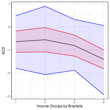
(b) Fully Nonparametric Model.

Figure 8. One-Sided Confidence Bounds for the ACD by Income Brackets.

Note: Estimate (black), bounds (red), and confidence bounds (blue) for the ACD. Confounding scenario: $\rho^{2}=1$; $C^{2}_{Y}=0.03$; $C^{2}_{D}\approx 0.03$. Significance level of 5%.

The second part of Table 3 reports the robustness values for price elasticity, such that the sensitivity bounds would contain a target value $\theta$. Here we consider $\theta=-1.5$ (very elastic) and $\theta=0$ (perfectly inelastic). We find that, at the 5% confidence level, these robustness values are at around 2% (PLM) and 1% (NPM). These results show that, unless researchers are able to rule out confounding that explains at about 2% of the residual variation of gasoline price and gasoline consumption, the evidence provided by the data is not strong enough to distinguish between extremes such as a “very elastic,” or a “perfectly inelastic” demand function. To put this number in context, our coarse measure of income (median of the income bracket) explains around 15% of the residual variation of gasoline price and 7% of the residual variation of gasoline demand. It is thus not implausible that remnant variation in the true income could overturn these results.

Finally, we explore how price elasticity varies with income under a specific confounding scenario. We consider three overlapping income groups defined as observations with income within $\pm.5$ in log-scale around the income points $\$42,500$, $\$57,500$ and $\$72,500$, as well as a fourth high income group of all units with income above $11.6$ on the log scale ($\approx\$110,000$). To illustrate, we consider a confounding scenario of approximately 3% for both sensitivity parameters, and repeat our non-parametric and partially linear estimation and sensitivity analysis for each sub-group. Point-estimates, bounds and confidence bounds are reported in Figure 8. Note that, under this scenario, the evidence for effect heterogeneity is substantially weakened, especially when using a fully non-parametric model. Sensitivity contour plots for the gasoline demand example, both for the partially linear model and the fully non-parametric model, are provided in Figures 9 and 10.

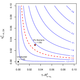
(a) Contours lower limit confidence bound (PLM).

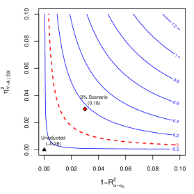
(b) Contours upper limit confidence bound (PLM).

Figure 9. Sensitivity contours gasoline demand, PLM. Significance level $a=0.05$.

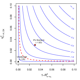
(a) Contours lower limit confidence bound (NPM).

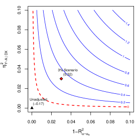
(b) Contours upper limit confidence bound (NPM).

Figure 10. Sensitivity contour plots gasoline demand, NPM. Significance level $a=0.05$.

6. Discussion

In this paper we provide sharp bounds on the size of omitted variable bias for continuous linear functionals of the conditional expectation function of the outcome—all for general, non-parametric, causal models. In particular, we allow for arbitrary (e.g., binary or continuous) treatment and outcome variables, and we show that the bounds on the bias depends only on the additional gains in variation that latent variables create both in the outcome regression, via the parameter $\eta_{Y\sim A\mid DX}$, and in the Riesz representer of the target functional, via the parameter $1-R^{2}_{\alpha\sim\alpha_{s}}$. Moreover, since $\eta_{Y\sim A\mid DX}\in[0,1]$, plausibility judgments on $1-R^{2}_{\alpha\sim\alpha_{s}}$ alone are sufficient to bound the target parameter of interest. We also provide theoretical details of important leading examples. In particular we derive novel bounds for the important special cases of average treatment effects in partially linear models, and in nonparametric models with a binary treatment. Finally, we leverage the Riesz representation of our bounds to offer flexible statistical inference through (debiased) machine learning, with rigorous coverage guarantees. Therefore, we provide a concise and complete solution to the problem of bounding the size of OVB, as well performing statistical inference on these bounds, for a rich and important class of causal parameters.

We now provide a brief discussion of the related literature on sensitivity analysis, as well as suggestions for possible extensions and future work. We focus the discussion on recent methods, and on how they differ from our proposal. We refer readers to Liu et al. (2013), Richardson et al. (2014), Cinelli and Hazlett (2020a), and Scharfstein et al. (2021) for further details.

6.1. Related literature

In contrast to our approach, many of the earlier works on sensitivity analyses demand from users a rather extensive specification, or parameterization, of the nature of unobserved confounders. This could range from positing the marginal (or conditional) distribution of these latent variables, along with specifying how such confounders would enter the outcome or treatment equations (e.g, entering linearly). Among such proposals, with varying degrees of requirements and parametric assumptions, we can find, e.g, Rosenbaum and Rubin (1983b), Imbens (2003), Vanderweele and Arah (2011), Dorie et al. (2016), Altonji et al. (2005), and Veitch and Zaveri (2020).

Another branch of the sensitivity literature requires users to specify instead a “tilting,” “selection,” or “bias” function, directly parameterizing the difference between the conditional distribution of the outcome under treatment (control) between treated and control units; or, when the target parameter is the ATE, just parameterizing the difference in conditional means. Earlier work on this area goes back to Robins (1999), Brumback et al. (2004), and Blackwell (2013), with more recent works from Franks et al. (2020) and Scharfstein et al. (2021), the latter with a special focus on binary treatments, and flexible semi-parametric estimation procedures. Our proposal differs from this literature in that we do not model the bias directly, instead we impose constraints on the maximum explanatory power of confounders.

Continuing with binary treatments, many sensitivity proposals focus on this special case. They differ mainly on how to parameterize departures from random assignment. For instance, Masten and Poirier (2018) places bounds on the difference between the treatment assignment distribution, conditioning and not conditioning on potential outcomes, whereas Rosenbaum (1987, 2002) and more recently Tan (2006); Yadlowsky et al. (2018); Kallus and Zhou (2018); Kallus et al. (2019); Zhao et al. (2019); Jesson et al. (2021) place bounds on the odds of such distributions. Bonvini and Kennedy (2021), on the other hand, propose a contamination model approach, placing restriction on the proportion of confounded units. Our approach is different from all these approaches in at least two main ways. First, we do not restrict our analyses to the binary treatment case. Second, even in the important case of a binary treatment, we parameterize violations of ignorability via the gains in precision, due to omitted variables, when predicting treatment assignment. Our sensitivity parameters and bounds are thus different from these approaches (we provide a numerical example in Appendix C.1, which demonstrates practical and theoretical value of the new parameterization).

Other sensitivity results, while allowing for general confounders, treatments and outcomes, restrict their attention to specific target parameters. For example, Ding and VanderWeele (2016) derive general bounds for the risk-ratio, with sensitivity parameters also in terms of risk-ratios. Our approach is thus different both in terms of target parameters (continuous linear functionals of the CEF), and in terms of sensitivity parameters ($R^{2}$ based sensitivity parameters). Cinelli and Hazlett (2020a) derive bounds for linear regression coefficients. Their result is a special case of ours when the target functional is the coefficient of a linear projection. Their approach does not cover nonlinear regression and the causal parameters that we study here (e.g, it does not cover the ATE in the nonparametric model with a binary treatment). Finally, Detommaso et al. (2021) provide an alternative expression for omitted variable bias of average causal derivatives, but they do not provide the sharp interpretable bounds, nor statistical inference for the bounds.

6.2. Possible extensions and future work

While throughout the paper we focus on bounding biases due to unmeasured confounding, we note that the same strategy we employ here can potentially be extended to bound biases due to misspecification errors, sampling selection, missing data, generalization of experimental results, imperfect instruments, among many other problems faced by empirical economists.

Consider, for example, the case of biased survey sampling. Suppose the target parameter is the population mean ${\mathrm{E}}Y$, and we may believe that the sampling selection process $S$ is only ignorable when conditioning on observed covariates $X$ and unobserved covariates $A$. We then have that the long parameter is $\theta:={\mathrm{E}}[{\mathrm{E}}[Y|X,A,S=1]]$ and the short parameter is $\theta_{s}:={\mathrm{E}}[{\mathrm{E}}[Y|X,S=1]]$. One can thus extend our results to bound survey biases using similar tools for bounding average potential outcomes provided in Section 3.

Our results can also be potentially extended to nonlinear functionals, such as those arising in instrumental variable (IV) methods. For instance, consider a variant of the IV problem (Imbens and Angrist, 1994), where the instrumental variable $Z$ is valid only when conditioning both on observed covariates $X$, and latent variables $A$. In this case, the IV estimand is given by the ratio of two average treatment effects,

$$\mathrm{IV}=\frac{\text{ATE}(Z\to Y)}{\text{ATE}(Z\to D)}.$$

Both the numerator and denominator can be bounded using the methods for the ATE proposed in this paper.

Another interesting direction for future work is to consider causal estimands that are functionals of the long quantile regression, or causal estimands that are values of a policy in dynamic stochastic programming. When the degree of confounding is small, it seems possible to use the results in Chernozhukov et al. (2022a) to derive approximate bounds on the bias that can be estimated using debiased ML approaches. A final suggestion for future studies is to investigate the use of shape restrictions on the long regression $g$ that can potentially sharpen the bounds.

Data Availability, Conflict of Interests, and Funding

Data availability.

All data is is publicly available in our GitHub repository: https://github.com/carloscinelli/dml.sensemakr.

Conflict of interest.

There are no relevant financial or nonfinancial competing interests to report.

Funding.

This research received no external funding.

Appendix A Preliminaries

A.1. Few Preliminaries

To prove supporting lemmas we recall the following definitions and results. Given two normed vector spaces $V$ and $W$ over the field of real numbers $\mathbb{R}$, a linear map $A:V\to W$ is continuous if and only if it has a bounded operator norm:

$$\|A\|_{op}:=\inf\{c\geq 0:\|Av\|\leq c\|v\|{\mbox{ for all }}v\in V\}<\infty,$$

where $\|\cdot\|_{op}$ is the operator norm. The operator norm depends on the choice of norms for the normed vector spaces $V$ and $W$. A Hilbert space is a complete linear space equipped with an inner product $\langle f,g\rangle$ and the norm $|\langle f,f\rangle|^{1/2}$. The space $L^{2}(P)$ is the Hilbert space with the inner product $\langle f,g\rangle=\int fgdP$ and norm $\|f\|_{P,2}$. The closed linear subspaces of $L^{2}(P)$ equipped with the same inner product and norm are Hilbert spaces.

Hahn-Banach Extension for Normed Vector Spaces. If $V$ is a normed vector space with linear subspace $U$ (not necessarily closed) and if $\phi:U\mapsto K$ is continuous and linear, then there exists an extension $\psi:V\mapsto K$ of $\phi$ which is also continuous and linear and which has the same operator norm as $\phi$.

Riesz-Frechet Representation Theorem. Let $H$ be a Hilbert space over $\mathbb{R}$ with an inner product $\langle\cdot,\cdot\rangle$, and $T$ a bounded linear functional mapping $H$ to $\mathbb{R}$. If $T$ is bounded then there exists a unique $g\in H$ such that for every $f\in H$ we have $T(f)=\langle f,g\rangle$. It is given by $g=z(Tz)$, where $z$ is unit-norm element of the orthogonal complement of the kernel subspace $K=\{a\in H:Ta=0\}$. Moreover, $\|T\|_{op}=\|g\|$, where $\|T\|_{op}$ denotes the operator norm of $T$, while $\|g\|$ denotes the Hilbert space norm of $g$.

Radon-Nykodym Derivative. Consider a measure space $(\mathcal{X},\mathcal{A})$ on which two $\sigma$-finite measure are defined, $\mu$ and $\nu$. If $\nu\ll\mu$ (i.e. $\nu$ is absolutely continuous with respect to $\mu$), then there is a measurable function $f:\mathcal{X}\rightarrow[0,\infty)$, such that for any measurable set $A\subseteq\mathcal{X}$, $\nu(A)=\int_{A}f\,d\mu$. The function $f$ is conventionally denoted by $d\nu/d\mu$.

Integration by Parts. Consider a closed measurable subset $\mathcal{X}$ of $\mathbb{R}^{k}$ equipped with Lebesgue measure $V$ and piecewise smooth boundary $\partial\mathcal{X}$, and suppose that $v:\mathcal{X}\to\mathbb{R}^{k}$ and $\phi:\mathcal{X}\to\mathbb{R}$ are both $C^{1}(\mathcal{X})$, then

$${\displaystyle\int_{\mathcal{X}}\varphi\operatorname{div}{{v}}\,dV=\int_{\partial\mathcal{X}}\varphi\,{{v}}^{\prime}nd{{S}}-\int_{\mathcal{X}}{{v}}^{\prime}\operatorname{grad}\varphi\,dV,}$$

where $S$ is the surface measure over the surface $\partial\mathcal{X}$ induced by $V$, and $n$ is the outward normal vector.

Appendix B Deferred Proofs

B.1. Proof of Theorem 1 and Corollary 1

The result follows from

$${\mathrm{E}}g\alpha-{\mathrm{E}}g_{s}\alpha_{s} = {\mathrm{E}}(g_{s}+g-g_{s})(\alpha_{s}+\alpha-\alpha_{s})-{\mathrm{E}}g_{s}\alpha_{s}$$

$$= {\mathrm{E}}g_{s}(\alpha-\alpha_{s})+{\mathrm{E}}\alpha_{s}(g-g_{s})+{\mathrm{E}}(g-g_{s})(\alpha-\alpha_{s})$$

$$= {\mathrm{E}}(g-g_{s})(\alpha-\alpha_{s}),$$

using the fact that $\alpha_{s}$ is orthogonal to $g-g_{s}$ and $g_{s}$ is orthogonal to $\alpha-\alpha_{s}$ by definition of $\alpha,\alpha_{s}$ and $g_{s}$.

To show the bound $|{\mathrm{E}}(g-g_{s})(\alpha-\alpha_{s})|^{2}\leq{\mathrm{E}}(g-g_{s})^{2}{\mathrm{E}}(\alpha-\alpha_{s})^{2}$ is sharp, we need to show that

$$1=\max\{\rho^{2}\mid(\alpha,g):{\mathrm{E}}(\alpha-\alpha_{s})^{2}=B^{2}_{\alpha},\quad{\mathrm{E}}(g-g_{s})^{2}=B^{2}_{g}\},$$

where $B_{\alpha}$ and $B_{g}$ are nonnegative constants such that $B^{2}_{g}\leq{\mathrm{E}}(Y-g_{s})^{2}$, and $\rho^{2}=\mathrm{Cor}^{2}(g-g_{s},\alpha-\alpha_{s})$. To do so, choose $g=g_{s}+A$, where $A$ is square-integrable and independent of $X$ such that ${\mathrm{E}}(g-g_{s})^{2}=B^{2}_{g}$, then set

$$\alpha-\alpha_{s}=B_{\alpha}(g-g_{s})/B_{g}.$$

This yields an admissible RR, and sets $\rho^{2}=1$.

Corollary 1 follows from observing that the bound factorizes as

$$B^{2}=S^{2}C^{2}_{Y}C^{2}_{D},$$

where $S^{2}:={\mathrm{E}}(Y-g_{s})^{2}{\mathrm{E}}\alpha_{s}^{2}$, and

$$C^{2}_{Y}=\frac{{\mathrm{E}}(g-g_{s})^{2}}{{\mathrm{E}}(Y-g_{s})^{2}}=R^{2}_{Y-g_{s}\sim g-g_{s}},$$

and

$$C^{2}_{D}=\frac{{\mathrm{E}}(\alpha-\alpha_{s})^{2}}{{\mathrm{E}}\alpha_{s}^{2}}=\frac{{\mathrm{E}}\alpha^{2}-{\mathrm{E}}\alpha^{2}_{s}}{{\mathrm{E}}\alpha_{s}^{2}}=\frac{1/{\mathrm{E}}\tilde{D}^{2}-1/{\mathrm{E}}\tilde{D}_{s}^{2}}{1/{\mathrm{E}}\tilde{D}_{s}^{2}}=\frac{{\mathrm{E}}\tilde{D}^{2}_{s}-{\mathrm{E}}\tilde{D}^{2}}{{\mathrm{E}}\tilde{D}^{2}}=\frac{R^{2}_{\tilde{D}_{s}\sim\tilde{A}}}{1-R^{2}_{\tilde{D}_{s}\sim\tilde{A}}},$$

where $\tilde{D}:=D-{\mathrm{E}}[D\mid X,A]$, $\tilde{D}_{s}:=D-{\mathrm{E}}[D\mid X]$, and $\tilde{A}={\mathrm{E}}[D\mid X,A]-{\mathrm{E}}[D\mid X]$.

Here we used the observation that

$${\mathrm{E}}(\alpha-\alpha_{s})^{2}={\mathrm{E}}\alpha^{2}+{\mathrm{E}}\alpha^{2}_{s}-2{\mathrm{E}}\alpha\alpha_{s}={\mathrm{E}}\alpha^{2}-{\mathrm{E}}\alpha^{2}_{s},$$

holds because

$${\mathrm{E}}\alpha\alpha_{s}=\frac{{\mathrm{E}}\tilde{D}\tilde{D}_{s}}{{\mathrm{E}}\tilde{D}^{2}{\mathrm{E}}\tilde{D}_{s}^{2}}=\frac{{\mathrm{E}}\tilde{D}^{2}}{{\mathrm{E}}\tilde{D}^{2}{\mathrm{E}}\tilde{D}_{s}^{2}}=\frac{1}{{\mathrm{E}}D^{2}_{s}}={\mathrm{E}}\alpha^{2}_{s}.$$

The corollary now follows immediately from the definitions of $\eta^{2}$, since

$$R^{2}_{Y-g_{s}\sim g-g_{s}}=\eta^{2}_{Y\sim A\mid D,X}\text{ and }R^{2}_{\tilde{D}_{s}\sim\tilde{A}}=\eta^{2}_{D\sim A\mid X}.$$

In addition, we note

$$\frac{{\mathrm{E}}\alpha^{2}-{\mathrm{E}}\alpha^{2}_{s}}{{\mathrm{E}}\alpha_{s}^{2}}=\frac{{\mathrm{E}}\alpha^{2}-{\mathrm{E}}\alpha^{2}_{s}}{{\mathrm{E}}\alpha^{2}}\frac{{\mathrm{E}}\alpha^{2}}{{\mathrm{E}}\alpha_{s}^{2}}=\frac{1-R^{2}_{\alpha\sim\alpha_{s}}}{R^{2}_{\alpha\sim\alpha_{s}}}.\qed$$

Remark 7 (Rationalization of any $\rho$ and $B^{2}_{g}$, and $B^{2}_{\alpha}$).

The above argument can be modified to show that we can achieve any $-1\leq\rho\leq 1$, $0\leq B^{2}_{\alpha}$, and $0\leq B^{2}_{g}\leq\operatorname{Var}(Y-g_{s})$ by a suitable confounding model as follows. Choose

$$g-g_{s}=\mu_{1}^{\prime}A\text{ and }\alpha-\alpha_{s}=\mu_{2}^{\prime}A,$$

where $A\sim N(0,I_{2})$, independently of $X$. Then set

$$\left(\begin{array}[]{c}\mu_{1}^{\prime}\\ \mu_{2}^{\prime}\end{array}\right)=\left(\begin{array}[]{cc}B_{g}^{2}&\rho B_{g}B_{\alpha}\\ \rho B_{g}B_{\alpha}&B^{2}_{\alpha}\end{array}\right)^{1/2}.\qed$$

Remark 8 (On “Natural” Confounding).

The preceding remark suggests a way to generate models of “natural confounding” that are not strictly adversarial and then calculate the expected R-squared $\rho^{2}$ given some “natural priors” on the model’s hyper-parameters. Consider the confounding model: $g-g_{s}=\mu_{1}^{\prime}A\text{ and }\alpha-\alpha_{s}=\mu_{2}^{\prime}A,$ where $A\sim N(0,I_{K})$ is $K$-dimensional vector of confounders. Suppose the hyperparameters $\mu$ are drawn from $N(0,I)$, then ${\mathrm{E}}\rho^{2}=1/K$, which attains maximal value of $1$ when $K=1$ and decreases to $0$ as $K\to\infty$. Therefore, there does not appear to exist a good formal way to set the level of “natural” confounding. ∎

B.2. Proof of Lemma 1

The existence of the unique long RR $\alpha\in L^{2}(P_{W})$ follows from the Riesz-Frechet representation theory. To show that we can take $\alpha_{s}(W^{s}):={\mathrm{E}}[\alpha(W)\mid W^{s}]$ to be the short RR, we first observe that the long RR obeys

$${\mathrm{E}}m(W,g_{s})={\mathrm{E}}g_{s}(W^{s})\alpha(W)$$

for all $g_{s}\in L^{2}(P_{W^{s}})$. That is, the long RR $\alpha$ can represent the linear functionals over the smaller space $L^{2}(P_{W^{s}})\subset L^{2}(P_{W})$, but $\alpha$ itself is not in $L^{2}(P_{W^{s}})$. Then, we decompose the long RR into the orthogonal projection $\alpha_{s}$ and the residual $e$:

$$\alpha(W)=\alpha_{s}(W^{s})+e(W);\quad{\mathrm{E}}e(W)g_{s}(W)=0,\text{ for all $g_{s}$ in }L^{2}(P_{W^{s}}).$$

Then

$${\mathrm{E}}g_{s}(W)\alpha(W) = {\mathrm{E}}\big{[}g_{s}(W^{s})\big{(}\alpha_{s}(W^{s})+e(W^{s})\big{)}\big{]}$$

$$= {\mathrm{E}}\big{[}g_{s}(W^{s})\alpha_{s}(W^{s})\big{]}.$$

Therefore ${\mathrm{E}}[\alpha(W)\mid W^{s}]$ is a short RR, and it is unique in $L^{2}(P_{W^{s}})$ by the RF theory. We also have that ${\mathrm{E}}\alpha^{2}={\mathrm{E}}\alpha^{2}_{s}+{\mathrm{E}}e^{2}$, establishing that ${\mathrm{E}}\alpha^{2}\geq{\mathrm{E}}\alpha^{2}_{s}$.∎

B.3. Proof of Lemma 2.

We have from the Riesz-Frechet theory that

$${\mathrm{E}}m(W,g_{r})={\mathrm{E}}g_{r}(W)\alpha(W),$$

for all $g_{r}\in\Gamma$, that is the RR $\alpha$ continues to represent the functional over the restricted linear subspace $\Gamma\subset L^{2}(P_{W})$. Decompose $\alpha$ in the orthogonal projection $\bar{\alpha}$ and the residual $e$:

$$\alpha(W)=\bar{\alpha}(W)+e(W),\quad{\mathrm{E}}e(W)g_{r}(W)=0,\text{ for all $g_{r}$ in }\Gamma.$$

Then we have that

$${\mathrm{E}}g_{r}(W)\alpha(W)={\mathrm{E}}g_{r}(W)\bar{\alpha}(W)+{\mathrm{E}}g_{r}(W)e(W)={\mathrm{E}}g_{r}(W)\bar{\alpha}(W).$$

That is, $\bar{\alpha}$ is a RR, and it is unique in $\Gamma$ by the RF theory. We also have that ${\mathrm{E}}\alpha^{2}={\mathrm{E}}\bar{\alpha}^{2}+{\mathrm{E}}e^{2}$, establishing that ${\mathrm{E}}\alpha^{2}\geq{\mathrm{E}}\bar{\alpha}^{2}$.

Analogous argument yields the result for the closed linear subsets $\Gamma_{s}$ of $L^{2}(P_{W^{s}})$.

Here we show that $\bar{\alpha}_{s}$ is given by a projection of $\bar{\alpha}$ onto $\Gamma_{s}$. Indeed, $\bar{\alpha}$ represents the functionals over $\Gamma_{s}$ but it is not itself in $\Gamma_{s}$. However, its projection onto $\Gamma_{s}$ therefore can also represent the functionals, using the same arguments as above. By uniqueness of the RR over $\Gamma_{s}$, we must have that the projected $\bar{\alpha}$ coincides with $\bar{\alpha}_{s}$. Further,

$${\mathrm{E}}(\bar{\alpha}-\bar{\alpha}_{s})^{2}\geq\min_{b\in\mathbb{R}}{\mathrm{E}}(\bar{\alpha}-b\bar{\alpha}_{s})^{2}\geq\min_{a\in\Gamma_{s}}{\mathrm{E}}(\bar{\alpha}-a)^{2}={\mathrm{E}}(\bar{\alpha}-\bar{\alpha}_{s})^{2}.$$

This shows that the linear orthogonal projection of $\bar{\alpha}$ on $\bar{\alpha}_{s}$ is given by $\bar{\alpha}_{s}$. The latter means that we can decompose:

$${\mathrm{E}}(\bar{\alpha}-\bar{\alpha}_{s})^{2}={\mathrm{E}}\alpha^{2}-{\mathrm{E}}\alpha^{2}_{s}.\qed$$

B.4. Proof of Theorem 2 and Corollary 2

We decompose $L^{2}(P_{W})$ into $L^{2}(P_{W^{s}})$ and its orthocomplement $L^{2}(P_{W^{s}})^{\perp}$,

$$L^{2}(P_{W})=L^{2}(P_{W^{s}})+L^{2}(P_{W^{s}})^{\perp}.$$

So that any element $m_{s}\in L^{2}(P_{W^{s}})$ is orthogonal to any $e\in L^{2}(P_{W^{s}})^{\perp}$ in the sense that

$${\mathrm{E}}m_{s}(W^{s})e(W)=0.$$

The claim of the theorem follows from

$${\mathrm{E}}g\alpha-{\mathrm{E}}g_{s}\alpha_{s} = {\mathrm{E}}(g_{s}+g-g_{s})(\alpha_{s}+\alpha-\alpha_{s})-{\mathrm{E}}g_{s}\alpha_{s}$$

$$= {\mathrm{E}}g_{s}(\alpha-\alpha_{s})+{\mathrm{E}}\alpha_{s}(g-g_{s})+{\mathrm{E}}(g-g_{s})(\alpha-\alpha_{s})$$

$$= {\mathrm{E}}(g-g_{s})(\alpha-\alpha_{s}),$$

using the fact that $\alpha_{s}\in L^{2}(P_{W^{s}})$ is orthogonal to $g-g_{s}\in L^{2}(P_{W^{s}})^{\perp}$ and $g_{s}\in L^{2}(P_{W^{s}})$ is orthogonal to $\alpha-\alpha_{s}\in L^{2}(P_{W^{s}})^{\perp}$.

Corollary 2 follows from observing that

$$\frac{{\mathrm{E}}(g-g_{s})^{2}}{{\mathrm{E}}(Y-g_{s})^{2}}=R^{2}_{Y-g_{s}\sim g-g_{s}},$$

as before, and from

$$\frac{{\mathrm{E}}(\alpha-\alpha_{s})^{2}}{{\mathrm{E}}\alpha_{s}^{2}}=\frac{{\mathrm{E}}\alpha^{2}-{\mathrm{E}}\alpha^{2}_{s}}{{\mathrm{E}}\alpha_{s}^{2}}=\frac{{\mathrm{E}}\alpha^{2}-{\mathrm{E}}\alpha^{2}_{s}}{{\mathrm{E}}\alpha^{2}}\frac{{\mathrm{E}}\alpha^{2}}{{\mathrm{E}}\alpha_{s}^{2}}=\frac{1-R^{2}_{\alpha\sim\alpha_{s}}}{R^{2}_{\alpha\sim\alpha_{s}}}.$$

The proof for the case where $g$’s and $\alpha$’s are restricted follows similarly, replacing $L^{2}(P_{W})$ with $\Gamma\subset L^{2}(P_{W})$ and $L^{2}(P_{W^{s}})$ with $\Gamma_{s}=\Gamma\cap L^{2}(P_{W_{s}})$, and decomposing $\Gamma=\Gamma_{s}+\Gamma_{s}^{\perp}$, where $\Gamma_{s}^{\perp}$ is the orthogonal complement of $\Gamma_{s}$ relative to $\Gamma$. The remaining arguments are the same, utilizing Lemma 2.

To show the bound is sharp we need to show that

$$1=\max\{\rho^{2}\mid(\alpha,g):{\mathrm{E}}(\alpha-\alpha_{s})^{2}=B^{2}_{\alpha},\quad{\mathrm{E}}(g-g_{s})^{2}=B^{2}_{g}\},$$

where $B_{\alpha}$ and $B_{g}$ are nonnegative constants such that $B^{2}_{g}\leq{\mathrm{E}}(Y-g_{s})^{2}$. To do so, choose any $\alpha$ such such that ${\mathrm{E}}(\alpha-\alpha_{s})^{2}=B^{2}_{\alpha}$, then set

$$g-g_{s}=B_{g}(\alpha-\alpha_{s})/B_{\alpha}.$$

This yields an admissible long regression function, and sets $\rho^{2}=1$. ∎

Remark 9.

We note here that distribution of observed data $P$ can place other restrictions on the problem, restricting admissible values of $B^{2}_{\alpha}$ or $B^{2}_{g}$ or $\rho^{2}<1$. For example, we have $0\leq g,g_{s}\leq 1$ when $0\leq Y\leq 1$. This implies $\|g-g_{s}\|_{\infty}\leq 1$, which can potentially result in the adversarial $\rho^{2}<1.$ ∎

We also note that Remark 7 applies here as well.

B.5. Proof of Theorem 3

Here the argument is similar to Chernozhukov et al. (2018b), but we provide details for completeness.

The assumptions directly imply that the candidate long RR obey $\alpha\in L^{2}(P)$ with $\|\alpha\|_{P,2}\leq C$ in each of the examples, for some constant $C$ that depends on $P$. By ${\mathrm{E}}Y^{2}<\infty$, we have $g\in L^{2}(P)$. Therefore, $|{\mathrm{E}}\alpha g|<\|\alpha\|_{P,2}\|g\|_{P,2}<\infty$ in any of the calculations below.

We first verify that long RR $\alpha$’s can indeed represent the functionals $g\mapsto\theta(g):={\mathrm{E}}m(W,g)$ in Examples 1,2,3,5 over $g\in L^{2}(P)$. In Example 4, the long RR represents the Hanh-Banach extension of the mapping $g\mapsto\theta(g)$ to $L^{2}(P)$ over $L^{2}(P)$.

In Example 1, recall that $\bar{\ell}(X,A):={\mathrm{E}}[\ell(W^{s})|X,A]$. Then since $dP(d,x,a)=\sum_{j=0}^{1}1(j=d)P[D=j|X=x,A=a]dP(x,a)$ by the Bayes rule, we have

$${\mathrm{E}}g(W)\alpha(W) = \int g(d,x,a)\frac{1(d=\bar{d})\bar{\ell}(x,a)}{P[D=\bar{d}|X=x,A=a]}dP(d,x,a)$$

$$= \int g(\bar{d},x,a)\bar{\ell}(x,a)dP(x,a)$$

$$= {\mathrm{E}}g(\bar{d},X,A)\bar{\ell}(X,A)={\mathrm{E}}g(\bar{d},X,A)\ell(W^{s})=\theta(g),$$

where the penultimate equality follows by the law of iterated expectations. The claim for Example 2 follows from the claim for Example 1.

Example 3 follows by the change of measure of $dP_{\tilde{W}}$ to $dP_{W}$, given the assumed absolutely continuity of the former with respect to the latter. Then we have

$${\mathrm{E}}g(W)\alpha(W) = \int g\ell\left(\frac{dP_{\tilde{W}}-dP_{W}}{dP_{W}}\right)dP_{W}=\int g\ell(dP_{\tilde{W}}-dP_{W})$$

$$= \int\ell(w^{s})(g(T(w^{s}),a)-g(w^{s},a))dP_{W}(w)=\theta(g).$$

In Example 4, we can write for any $g^{\prime}s$ that have the properties stated in this example:

$${\mathrm{E}}g(W)\alpha(W) = -\int\int g(w)\frac{\mathrm{div}_{d}(\ell(w^{s})t(w^{s})f(d|x,a))}{f(d|x,a)}f(d|x,a)\mathrm{d}d\mathrm{d}P(x,a)$$

$$= -\int\int g(w)\mathrm{div}_{d}(\ell(w^{s})t(w^{s})f(d|x,a))\mathrm{d}d\mathrm{d}P(x,a)$$

$$= -\int\int_{\partial\mathcal{D}_{a,x}}g(w)t(w^{s})^{\prime}\ell(w^{s})f(d|x,a)n_{a,x}(d)\mathrm{d}S(d)\mathrm{d}P(x,a)$$

$$+\int\int\partial_{d}g(w)^{\prime}t(w^{s})\ell(w^{s})f(d|x,a)\mathrm{d}d\mathrm{d}P(x,a)$$

$$= \ \int\int\partial_{d}g(w)^{\prime}t(w^{s})\ell(w^{s})f(d|x,a)\mathrm{d}d\mathrm{d}P(x,a)=\theta(g),$$

where we used the integration by parts and that $\ell(w^{s})t(w^{s})f(d|x,a)$ vanishes for any $d$ in the boundary of $\mathcal{D}_{x,a}$.

Example 5 follows by the change of measure $dP_{A}\times dF_{k}$ to $dP_{W}$, given the assumed absolutely continuity of the former with respect to the latter on $\mathcal{A}\times\text{support}(\ell)$. Then we have

$${\mathrm{E}}g(W)\alpha(W) = \int g\ell\left(\frac{[dP_{A}\times d(F_{1}-F_{0})]}{dP_{W}}\right)dP_{W}$$

$$= \int g(w^{s},a)\ell(w^{s})dP_{A}(a)d(F_{1}-F_{0})(w^{s})=\theta(g).$$

In all examples, the continuity of $g\mapsto\theta(g)$ required in Assumption 1 now follows from the representation property and from $|{\mathrm{E}}\alpha g|\leq\|\alpha\|_{P,2}\|g\|_{P,2}\leq C\|g\|_{P,2}$.

Verification of Assumption 2 follows directly from the inspection of m-scores given in Section 5.

Note that we do not need the analytical form of the short RRs to verify Assumptions 1 or 2. However, their analytical form can be found by exactly the same steps as above, or by taking the conditional expectation. ∎

B.6. Proof of Lemma 3 and Theorem 4

The Lemma follows from the application of Theorem 3.1 and Theorem 3.2 in Chernozhukov et al. (2018a). Valid estimation of covariance follows similarly to the proof of Theorem 3.2 in Chernozhukov et al. (2018a). The first result of Theorem 4 follows from the delta method in van der Vaart and Wellner (1996). The validity of the confidence intervals follows from using the standard arguments for confidence intervals based on asymptotic normality.∎

Appendix C Benchmarking Analysis

The ideas that inspire the comparisons we make here are in Imbens (2003); Altonji et al. (2005); Cinelli and Hazlett (2020a); Oster (2017). Our goal is to compare the confounding assumptions that we make regarding latent confounders to the observed strength of association of observed covariates. We consider the following observed confounders: (i) worker’s income (“income”); (ii) whether a worker has an individual retirement account (“IRA”); and (iii) whether the worker’s family has a two-earner status (“two-earners”). These observed covariates were chosen because of their financial nature, and they may be acting similarly to the effect of omitted firm characteristics via match amount.

From the tables reported below we see that, apart from income, the other covariates have weak explanatory power either with the outcome or with the treatment; in this sense, they are all weak “observed confounders,” and do not meaningfully change the estimated short parameter. Moreover, the observed effective correlation is much smaller than the adversarial correlation of $\rho=1$. In summary, the confounding scenario in the main text is more conservative than the ones suggested by benchmarks considered, other than income. Below we provide the formal details of the benchmarking analysis.

Notation. For a given observed covariate $X_{j}$, let $X_{-j}$ denotes the set of all other observed covariates $X$ except $X_{j}$. Let $g_{s,-j}$ and $\alpha_{s,-j}$ denote the CEF and the RR excluding covariate $X_{j}$. Let $\tilde{Y}=Y-g_{s}$ and $\tilde{Y}_{-j}=Y-g_{s,-j}$. Let $\Delta\eta^{2}_{Y\sim X_{j}}$ the observed additive gains in explanatory power of $X_{j}$ for $Y$: $\Delta\eta^{2}_{Y\sim X_{j}}:=\eta^{2}_{Y\sim DX}-\eta^{2}_{Y\sim DX_{-j}}.$ Similarly, let $\Delta\eta^{2}_{D\sim X_{j}}:=\eta^{2}_{D\sim X}-\eta^{2}_{D\sim X_{-j}}$ denote the additive gain in the explanatory power of $X_{j}$ for $D$, which will be used for PLM. More generally, we define the gain in the explanatory power of $X_{j}$ with the RR as:

$$1-R^{2}_{\alpha_{s}\sim\alpha_{s,-j}}=\frac{{\mathrm{E}}\alpha_{s}^{2}-{\mathrm{E}}\alpha_{s,-j}^{2}}{{\mathrm{E}}\alpha_{s}^{2}}.$$

We also define the change in the estimates of the ATE: $\Delta\theta_{s,j}:={\mathrm{E}}m(W,g_{s,-j})-{\mathrm{E}}m(W,g_{s})$, for $m(w,g):=g(1,X)-g(0,X)]$, and the degree of adversity:

$$\rho_{j}=\mathrm{Cor}(g_{s,-j}-g_{s},\alpha_{s}-\alpha_{s,-j}).$$

Benchmarking Model. Similar in spirit to the analysis of Cinelli and Hazlett (2020a) for linear regression, our benchmarking model postulates the following hypotheses, relating the strength of unobserved confounders to that of the observed ones.

For the strength of association with the outcome, we posit:

$$\eta^{2}_{Y\sim A\mid DX}\approx\frac{\eta_{Y\sim X_{j}\mid DX_{-j}}^{2}}{1-\eta_{Y\sim X_{j}\mid DX_{-j}}^{2}}=\frac{\Delta\eta_{Y\sim X_{j}}^{2}}{1-\eta_{Y\sim DX}^{2}}=:G_{Y,j}$$

Whereas for the strength of association with the RR, we posit:

$$1-R_{\alpha\sim\alpha_{s}}^{2}\approx\frac{1-R_{\alpha_{s}\sim\alpha_{s,-j}}^{2}}{R_{\alpha_{s}\sim\alpha_{s,-j}}^{2}}:=G_{D,j}.$$

In PLM, this corresponds to the following hypothesis:

$$1-R_{\alpha\sim\alpha_{s}}^{2}=\eta^{2}_{D\sim A\mid X}\approx\frac{\eta_{D\sim X_{j}\mid X_{-j}}^{2}}{1-\eta_{D\sim X_{j}\mid X_{-j}}^{2}}=\frac{\Delta\eta_{D\sim X_{j}}^{2}}{1-\eta_{D\sim X}^{2}}.$$

We call $G_{Y,j}$ and $G_{D,j}$ the gain metrics and report them in the tables reported below. They measure gains in the explanatory power of covariates and, under the stated hypotheses, serve as proxies for the key quantities $\eta^{2}_{Y\sim A\mid DX}$ and $1-R_{\alpha\sim\alpha_{s}}^{2}$ that we put on the axes in the sensitivity plots. The quantities also immediately pin-down $C_{Y}^{2}=\eta^{2}_{Y\sim A\mid DX}$ and $C_{D}^{2}=(1-R_{\alpha\sim\alpha_{s}}^{2})/R_{\alpha\sim\alpha_{s}}^{2}$ that enter the bias bounds formulas.

Remark 10 (Rationale).

Here is some rationale for the strategy above. We know that:

$$1-R_{\alpha\sim\alpha_{s}}^{2}=1-\frac{{\mathrm{E}}\alpha_{s}^{2}}{{\mathrm{E}}\alpha^{2}}.$$

Now dividing and multiplying by ${\mathrm{E}}\alpha_{s,-j}^{2}$ we obtain the following decomposition:

$$1-R_{\alpha\sim\alpha_{s}}^{2}=1-\frac{{\mathrm{E}}\alpha_{s}^{2}}{{\mathrm{E}}\alpha_{s,-j}^{2}}\frac{{\mathrm{E}}\alpha_{s,-j}^{2}}{E\alpha^{2}}=1-\frac{R_{\alpha\sim\alpha_{s,-j}}^{2}}{R_{\alpha_{s}\sim\alpha_{s,-j}}^{2}}$$

$$=\frac{R_{\alpha_{s}\sim\alpha_{s,-j}}^{2}-R_{\alpha\sim\alpha_{s,-j}}^{2}}{R_{\alpha_{s}\sim\alpha_{s,-j}}^{2}}=\frac{(1-R_{\alpha\sim\alpha_{s,-j}}^{2})-(1-R_{\alpha_{s}\sim\alpha_{s,-j}}^{2})}{R_{\alpha_{s}\sim\alpha_{s,-j}}^{2}}.$$

We can treat the numerator as the additive gain in variation that the latent variables $A$ create in the $\mathrm{RR}$, in addition to what $X_{j}$ creates. If we posit the gain $(1-R_{\alpha\sim\alpha_{s,-j}}^{2})-(1-R_{\alpha_{s}\sim\alpha_{s,-j}}^{2})$ is the same as the one observed due to the addition of $X_{j}$, namely $\approx(1-R_{\alpha_{s}\sim\alpha_{s,-j}}^{2})$, we obtain the result above:

$$1-R_{\alpha\sim\alpha_{s}}^{2}\approx\frac{1-R_{\alpha_{s}\sim\alpha_{s,-j}}^{2}}{R_{\alpha_{s}\sim\alpha_{s,-j}}^{2}}.$$

The rationale for benchmarking the gain in explanatory power for outcomes is similar. ∎

Debiased Representations. It is important to use debiased (Neyman orthogonal) representations for the components of the formulas above:

$$\eta^{2}_{Y\sim DX}=1-\frac{\operatorname{Var}(\tilde{Y})}{\operatorname{Var}(Y)},\quad\eta^{2}_{Y\sim DX_{-j}}=1-\frac{\operatorname{Var}(\tilde{Y}_{-j})}{\operatorname{Var}(Y)}.$$

$$\eta^{2}_{D\sim X}=1-\frac{\operatorname{Var}(\tilde{D})}{\operatorname{Var}(D)},\quad\eta^{2}_{D\sim X_{-j}}=1-\frac{\operatorname{Var}(\tilde{D}_{-j})}{\operatorname{Var}(D)},$$

where $\tilde{D}_{-j}:=D-{\mathrm{E}}[D\mid X_{-j}]$ and $\tilde{D}:=D-{\mathrm{E}}[D\mid X]$; $R^{2}_{\alpha_{s}\sim\alpha_{s,-j}}=\nu^{2}_{s,-j}/\nu^{2}_{s},$ where

$$\nu^{2}_{s}:=2{\mathrm{E}}m(W,\alpha_{s})-{\mathrm{E}}\alpha^{2}_{s}\text{ and }\nu^{2}_{s,-j}:=2{\mathrm{E}}m(W,\alpha_{s,-j})-{\mathrm{E}}\alpha^{2}_{s,-j}$$

are the debiased forms for ${\mathrm{E}}\alpha_{s}^{2}$ and ${\mathrm{E}}\alpha_{s,-j}^{2}$. The debiased form of the change in the estimates is

$$\Delta\theta_{s,j}={\mathrm{E}}m(W,g_{s,-j})+{\mathrm{E}}\tilde{Y}_{-j}\alpha_{s,-j}-{\mathrm{E}}m(W,g_{s})-{\mathrm{E}}\tilde{Y}\alpha_{s};$$

and the debiased representation for the degree of adversity is

$$\rho_{j}=\frac{\Delta\theta_{s,j}}{\sqrt{\operatorname{Var}(\tilde{Y}_{-j})-\operatorname{Var}(\tilde{Y})}\sqrt{\nu^{2}_{s}-\nu^{2}_{s,-j}}}.$$

Empirical Benchmarking Results. The following are the empirical results for the 401(k) example.

	Gain Metrics		Degree of Adversity	Change in estimate
Observed covariate	$G_{Y,j}$	$G_{D,j}$	$\rho_{j}$	$\Delta\widehat{\theta}_{s,j}$
inc	0.1684	0.0470	0.3378	3466.2412
pira	0.0597	0.0055	0.1767	379.3715
twoearn	0.0358	0.0083	-0.3111	-629.6034

Table 4. Explanatory power of observed covariates in Partially Linear Model. All estimates are debiased and cross-fitted.

	Gain Metrics		Degree of Adversity	Change in estimate
Observed covariate	$G_{Y,j}$	$G_{D,j}$	$\rho_{j}$	$\Delta\widehat{\theta}_{s,j}$
inc	0.1497	0.1352	0.2246	3801.0798
pira	0.0405	0.0045	0.3176	544.4482
twoearn	0.0156	0.0171	-0.2568	-526.4658

Table 5. Explanatory power of observed covariates in NPM Model. All estimates are debiased and cross-fitted.

C.1. Comparison with Rosenbaum’s and marginal sensitivity models

Given their popularity and importance, here we expand on the difference between our sensitivity parameters, and sensitivity parameters based on odds-ratios, such as in Rosenbaum’s sensitivity model and “marginal sensitivity models” (Rosenbaum, 2002; Tan, 2006; Kallus et al., 2019; Zhao et al., 2019). We note similar reasoning can be applied to risk-ratio based parameters, such as those in Ding and VanderWeele (2016).As these approaches usually restrict $D$ to be binary, we focus on this case, with the understanding that this is not necessary for our approach.

Let, $\pi(x):=P(D=1\mid X=x)$ denote the “short” propensity score, and $\pi_{d}(x,y):=P(D=1\mid X=x,Y(d)=y)$ denote the “long” propensity score, conditioning on the potential outcome $Y(d)$, $d\in\{0,1\}$. Also, let $\text{OR}(p_{1},p_{2})=\frac{p_{1}/(1-p_{1})}{p_{2}/(1-p_{2})}$ denote the odds ratio for any two probabilities $p_{1},p_{2}\in(0,1)$. The marginal sensitivity model places bounds on the sensitivity parameter $\text{OR}(\pi_{d}(x,y),\pi(x))$; namely, it posits $\Lambda\geq 1$ such that

$$\frac{1}{\Lambda}\leq\text{OR}(\pi_{d}(x,y),\pi(x))\leq\Lambda,\qquad\forall x\in\mathcal{X},y\in\mathcal{Y},d\in\{0,1\}$$

Similarly, Rosenbaum’s model places bounds on the sensitivity parameter $\text{OR}(\pi_{d}(x,y),\pi_{d}(x,y^{\prime}))$; that is, it posits $\Gamma\geq 1$ such that

$$\frac{1}{\Gamma}\leq\text{OR}(\pi_{d}(x,y),\pi_{d}(x,y^{\prime}))\leq\Gamma,\qquad\forall x\in\mathcal{X},y,y^{\prime}\in\mathcal{Y},d\in\{0,1\}$$

Note these sensitivity parameters are in terms of odds ratios and thus can be unbounded; our sensitivity parameters are given in terms of $R^{2}$ measures, and are constrained to be between zero and one. To illustrate, let the unobserved confounder $A$ be normally distributed, $A\sim N(0,0.1)$ and let $Y(d)=A$ for $d\in\{0,1\}$, that is, in truth there is no treatment effect of $D$ on $Y$. For simplicity, consider the case with no observed covariates $X$. Now let the full propensity score be

$$P(D=1\mid Y(d)=y) =\frac{e^{.1y}}{1+e^{.1y}}$$ (12)

We then have that $\text{OR}(\pi_{d}(x,y),\pi_{d}(x,y^{\prime}))=e^{.1(y-y^{\prime})}$ and $\text{OR}(\pi_{d}(x,y),\pi(x))=e^{.1y}$. Thus, the true $\Gamma$ and $\Lambda$ parameters are unbounded,

$$\Gamma=\Lambda=\infty.$$

In contrast, the true $1-R^{2}_{\alpha\sim\alpha_{s}}$ evaluates to (by numerical integration) $1-R^{2}_{\alpha\sim\alpha_{s}}\approx 0.25\%$.

In summary, in this example, the true sensitivity parameters translate into tight bounds on the ATE in our approach, versus uninformative bounds in odds-ratio based approaches. The example emphasizes the extreme differences that can arise between the two parameterizations, and underscores the potential value of our new approach for empirical work.

References

- Altonji et al. (2005) Joseph G Altonji, Todd E Elder, and Christopher R Taber. Selection on observed and unobserved variables: Assessing the effectiveness of catholic schools. Journal of political economy, 113(1):151–184, 2005.
- Angrist and Pischke (2009) Joshua D. Angrist and Jorn-Steffan Pischke. Mostly Harmless Econometrics: An Empiricist’s Companion. Princeton University Press, 2009.
- Bickel et al. (1993) Peter J Bickel, Chris AJ Klaassen, Ya’acov Ritov, and Jon A Wellner. Efficient and Adaptive Estimation for Semiparametric Models, volume 4. Johns Hopkins University Press, 1993.
- Blackwell (2013) Matthew Blackwell. A selection bias approach to sensitivity analysis for causal effects. Political Analysis, 22(2):169–182, 2013.
- Blundell et al. (2012) Richard Blundell, Joel L Horowitz, and Matthias Parey. Measuring the price responsiveness of gasoline demand: Economic shape restrictions and nonparametric demand estimation. Quantitative Economics, 3(1):29–51, 2012.
- Blundell et al. (2017) Richard Blundell, Joel Horowitz, and Matthias Parey. Nonparametric estimation of a nonseparable demand function under the slutsky inequality restriction. Review of Economics and Statistics, 99(2):291–304, 2017.
- Bonvini and Kennedy (2021) Matteo Bonvini and Edward H Kennedy. Sensitivity analysis via the proportion of unmeasured confounding. Journal of the American Statistical Association, pages 1–11, 2021.
- Brumback et al. (2004) Babette A Brumback, Miguel A Hernán, Sebastien JPA Haneuse, and James M Robins. Sensitivity analyses for unmeasured confounding assuming a marginal structural model for repeated measures. Statistics in medicine, 23(5):749–767, 2004.
- Chernozhukov et al. (2018a) Victor Chernozhukov, Denis Chetverikov, Mert Demirer, Esther Duflo, Christian Hansen, Whitney Newey, and James Robins. Double/debiased machine learning for treatment and structural parameters. The Econometrics Journal, 2018a. ArXiv 2016; arXiv:1608.00060.
- Chernozhukov et al. (2018b) Victor Chernozhukov, Whitney Newey, and Rahul Singh. De-biased machine learning of global and local parameters using regularized riesz representers. arXiv preprint arXiv:1802.08667, 2018b.
- Chernozhukov et al. (2020) Victor Chernozhukov, Whitney Newey, Rahul Singh, and Vasilis Syrgkanis. Adversarial estimation of riesz representers. arXiv preprint arXiv:2101.00009, 2020.
- Chernozhukov et al. (2021) Victor Chernozhukov, Whitney K Newey, Victor Quintas-Martinez, and Vasilis Syrgkanis. Automatic debiased machine learning via neural nets for generalized linear regression. arXiv preprint arXiv:2104.14737, 2021.
- Chernozhukov et al. (2022a) Victor Chernozhukov, Juan Carlos Escanciano, Hidehiko Ichimura, Whitney K Newey, and James M Robins. Locally robust semiparametric estimation. Econometrica, 2022a.
- Chernozhukov et al. (2022b) Victor Chernozhukov, Whitney K. Newey, Victor Quintas-Martinez, and Vasilis Syrgkanis. Riesznet and forestriesz: Automatic debiased machine learning with neural nets and random forests. International Conference on Machine Learning, 2022b.
- Chernozhukov et al. (2022c) Victor Chernozhukov, Whitney K Newey, and Rahul Singh. Automatic debiased machine learning of causal and structural effects. Econometrica, 2022c.
- Chetverikov and Wilhelm (2017) Denis Chetverikov and Daniel Wilhelm. Nonparametric instrumental variable estimation under monotonicity. Econometrica, 85(4):1303–1320, 2017. doi: https://doi.org/10.3982/ECTA13639.
- Chetverikov et al. (2018) Denis Chetverikov, Dongwoo Kim, and Daniel Wilhelm. Nonparametric instrumental-variable estimation. The Stata Journal, 18(4):937–950, 2018.
- Cinelli and Hazlett (2020a) Carlos Cinelli and Chad Hazlett. Making sense of sensitivity: Extending omitted variable bias. Journal of the Royal Statistical Society: Series B (Statistical Methodology), 82(1):39–67, 2020a.
- Cinelli and Hazlett (2020b) Carlos Cinelli and Chad Hazlett. An omitted variable bias framework for sensitivity analysis of instrumental variables. Work. Pap, 2020b.
- Cinelli et al. (2019) Carlos Cinelli, Daniel Kumor, Bryant Chen, Judea Pearl, and Elias Bareinboim. Sensitivity analysis of linear structural causal models. International Conference on Machine Learning, 2019.
- Cornfield et al. (1959) Jerome Cornfield, William Haenszel, E Cuyler Hammond, Abraham M Lilienfeld, Michael B Shimkin, and Ernst L Wynder. Smoking and lung cancer: recent evidence and a discussion of some questions. Journal of the National Cancer institute, 22(1):173–203, 1959.
- Detommaso et al. (2021) Gianluca Detommaso, Michael Brückner, Philip Schulz, and Victor Chernozhukov. Causal bias quantification for continuous treatment, 2021.
- Ding and VanderWeele (2016) Peng Ding and Tyler J VanderWeele. Sensitivity analysis without assumptions. Epidemiology (Cambridge, Mass.), 27(3):368, 2016.
- Doksum and Samarov (1995) Kjell Doksum and Alexander Samarov. Nonparametric estimation of global functionals and a measure of the explanatory power of covariates in regression. The Annals of Statistics, pages 1443–1473, 1995.
- Dorie et al. (2016) Vincent Dorie, Masataka Harada, Nicole Bohme Carnegie, and Jennifer Hill. A flexible, interpretable framework for assessing sensitivity to unmeasured confounding. Statistics in medicine, 35(20):3453–3470, 2016.
- Frank (2000) Kenneth A Frank. Impact of a confounding variable on a regression coefficient. Sociological Methods & Research, 29(2):147–194, 2000.
- Frank et al. (2013) Kenneth A Frank, Spiro J Maroulis, Minh Q Duong, and Benjamin M Kelcey. What would it take to change an inference? Using Rubin’s causal model to interpret the robustness of causal inferences. Educational Evaluation and Policy Analysis, 35(4):437–460, 2013.
- Franks et al. (2020) AlexanderM Franks, Alexander D’Amour, and Avi Feller. Flexible sensitivity analysis for observational studies without observable implications. Journal of the American Statistical Association, 115(532):1730–1746, 2020.
- Hasminskii and Ibragimov (1978) Rafail Z Hasminskii and Ildar A Ibragimov. On the nonparametric estimation of functionals. In Proceedings of the 2nd Prague Symposium on Asymptotic Statistics, pages 41–51, 1978.
- Hosman et al. (2010) Carrie A Hosman, Ben B Hansen, and Paul W Holland. The sensitivity of linear regression coefficients’ confidence limits to the omission of a confounder. The Annals of Applied Statistics, pages 849–870, 2010.
- Imai et al. (2010) Kosuke Imai, Luke Keele, Teppei Yamamoto, et al. Identification, inference and sensitivity analysis for causal mediation effects. Statistical science, 25(1):51–71, 2010.
- Imbens (2003) Guido W Imbens. Sensitivity to exogeneity assumptions in program evaluation. American Economic Review, 93(2):126–132, 2003.
- Imbens and Angrist (1994) Guido W. Imbens and Joshua D. Angrist. Identification and estimation of local average treatment effects. Econometrica, 62:467–475, 1994.
- Imbens and Manski (2004) Guido W Imbens and Charles F Manski. Confidence intervals for partially identified parameters. Econometrica, 72(6):1845–1857, 2004.
- Imbens and Rubin (2015) Guido W Imbens and Donald B Rubin. Causal inference in statistics, social, and biomedical sciences. Cambridge University Press, 2015.
- Jesson et al. (2021) Andrew Jesson, Sören Mindermann, Yarin Gal, and Uri Shalit. Quantifying ignorance in individual-level causal-effect estimates under hidden confounding. arXiv preprint arXiv:2103.04850, 2021.
- Kallus and Zhou (2018) Nathan Kallus and Angela Zhou. Confounding-robust policy improvement. arXiv preprint arXiv:1805.08593, 2018.
- Kallus et al. (2019) Nathan Kallus, Xiaojie Mao, and Angela Zhou. Interval estimation of individual-level causal effects under unobserved confounding. In The 22nd international conference on artificial intelligence and statistics, pages 2281–2290. PMLR, 2019.
- Levit (1975) Boris Ya Levit. On efficiency of a class of non-parametric estimates. Teoriya Veroyatnostei i ee Primeneniya, 20(4):738–754, 1975.
- Liu et al. (2013) Weiwei Liu, S Janet Kuramoto, and Elizabeth A Stuart. An introduction to sensitivity analysis for unobserved confounding in nonexperimental prevention research. Prevention science, 14(6):570–580, 2013.
- Masten and Poirier (2018) Matthew A Masten and Alexandre Poirier. Identification of treatment effects under conditional partial independence. Econometrica, 86(1):317–351, 2018.
- Newey (1994) Whitney K Newey. The asymptotic variance of semiparametric estimators. Econometrica: Journal of the Econometric Society, pages 1349–1382, 1994.
- ORNL (2004) Oak Ridge National Laboratory ORNL. 2001 national household travel survey: User guide. ORNL, 2004. URL http://nhts.ornl.gov/.
- Oster (2017) Emily Oster. Unobservable selection and coefficient stability: Theory and evidence. Journal of Business & Economic Statistics, pages 1–18, 2017.
- Pearl (2009) Judea Pearl. Causality. Cambridge university press, 2009.
- Pearson (1905) Karl Pearson. On the general theory of skew correlation and non-linear regression. Dulau and Company, 1905.
- Pfanzagl and Wefelmeyer (1985) J Pfanzagl and W Wefelmeyer. Contributions to a general asymptotic statistical theory. Statistics & Risk Modeling, 3(3-4):379–388, 1985.
- Poterba et al. (1994) James M. Poterba, Steven F. Venti, and David A. Wise. 401(k) plans and tax-deferred savings. In D. A. Wise, editor, Studies in the Economics of Aging. Chicago, IL: University of Chicago Press, 1994.
- Poterba et al. (1995) James M. Poterba, Steven F. Venti, and David A. Wise. Do 401(k) contributions crowd out other personal saving? Journal of Public Economics, 58:1–32, 1995.
- Richardson et al. (2014) Amy Richardson, Michael G Hudgens, Peter B Gilbert, and Jason P Fine. Nonparametric bounds and sensitivity analysis of treatment effects. Statistical Science, 29(4):596, 2014.
- Robins (1999) James M Robins. Association, causation, and marginal structural models. Synthese, 121(1):151–179, 1999.
- Rosenbaum (1987) Paul R Rosenbaum. Sensitivity analysis for certain permutation inferences in matched observational studies. Biometrika, 74(1):13–26, 1987.
- Rosenbaum (2002) Paul R Rosenbaum. Observational studies. In Observational studies, pages 1–17. Springer, 2002.
- Rosenbaum and Rubin (1983a) Paul R Rosenbaum and Donald B Rubin. The central role of the propensity score in observational studies for causal effects. Biometrika, 70(1):41–55, 1983a.
- Rosenbaum and Rubin (1983b) Paul R Rosenbaum and Donald B Rubin. Assessing sensitivity to an unobserved binary covariate in an observational study with binary outcome. Journal of the Royal Statistical Society. Series B (Methodological), pages 212–218, 1983b.
- Scharfstein et al. (2021) Daniel O Scharfstein, Razieh Nabi, Edward H Kennedy, Ming-Yueh Huang, Matteo Bonvini, and Marcela Smid. Semiparametric sensitivity analysis: Unmeasured confounding in observational studies. arXiv preprint arXiv:2104.08300, 2021.
- Semenova and Chernozhukov (2021) Vira Semenova and Victor Chernozhukov. Debiased machine learning of conditional average treatment effects and other causal functions. The Econometrics Journal, 24(2):264–289, 2021.
- Shpitser et al. (2012) Ilya Shpitser, Tyler VanderWeele, and James M Robins. On the validity of covariate adjustment for estimating causal effects. arXiv preprint arXiv:1203.3515, 2012.
- Stoye (2009) Jörg Stoye. More on confidence intervals for partially identified parameters. Econometrica, 77(4):1299–1315, 2009.
- Tan (2006) Zhiqiang Tan. A distributional approach for causal inference using propensity scores. Journal of the American Statistical Association, 101(476):1619–1637, 2006.
- Van der Laan and Rose (2011) Mark J Van der Laan and Sherri Rose. Targeted learning: causal inference for observational and experimental data. Springer Science & Business Media, 2011.
- van der Vaart and Wellner (1996) A. W. van der Vaart and J. A. Wellner. Weak Convergence and Empirical Processes. Springer Series in Statistics, 1996.
- Vanderweele and Arah (2011) Tyler J. Vanderweele and Onyebuchi A. Arah. Bias formulas for sensitivity analysis of unmeasured confounding for general outcomes, treatments, and confounders. Epidemiology (Cambridge, Mass.), 22(1):42–52, January 2011.
- VanderWeele and Ding (2017) Tyler J VanderWeele and Peng Ding. Sensitivity analysis in observational research: introducing the E-value. Annals of Internal Medicine, 167(4):268–274, 2017.
- Veitch and Zaveri (2020) Victor Veitch and Anisha Zaveri. Sense and sensitivity analysis: Simple post-hoc analysis of bias due to unobserved confounding. Advances in Neural Information Processing Systems, 33:10999–11009, 2020.
- Yadlowsky et al. (2018) Steve Yadlowsky, Hongseok Namkoong, Sanjay Basu, John Duchi, and Lu Tian. Bounds on the conditional and average treatment effect with unobserved confounding factors. arXiv preprint arXiv:1808.09521, 2018.
- Zhao et al. (2019) Qingyuan Zhao, Dylan S Small, and Bhaswar B Bhattacharya. Sensitivity analysis for inverse probability weighting estimators via the percentile bootstrap. Journal of the Royal Statistical Society: Series B, 81(4):735–761, 2019.