Study of charmless two-body baryonic $B$ decays

Abstract

We study the charmless two-body decays of $B\to{\bf B}_{n}\overline{\bf B}_{n}^{\prime}$ with $B=(B^{+},B^{0},B^{0}_{s})$ and ${\bf B}_{n}^{(\prime)}$ the low-lying octet baryons. The factorizable amplitudes are calculated by the modified bag model, while the nonfactorizable ones are extracted from the experimental data with the $SU(3)_{F}$ flavor symmetry. We are able to explain all current experimental measurements and provide predictions on the decay branching ratios in $B\to{\bf B}_{n}\overline{\bf B}_{n}^{\prime}$. Particularly, we find that ${\cal B}(B_{s}^{0}\to\Xi^{0}\overline{\Xi}^{0})=(32.5\pm 3.7)\times 10^{-7}$ and ${\cal B}(B_{s}^{0}\to\Xi^{-}\overline{\Xi}^{-})=(33.1\pm 3.8)\times 10^{-7}$, which are sizable and able to be observed in the ongoing experiments at LHCb and BELLE-II. Furthermore, the decay branching ratios of $B_{s}^{0}\to(p\overline{p},n\overline{n})$ and $B^{0}\to(\Xi^{0}\overline{\Xi}^{0},\Sigma^{+}\overline{\Sigma}^{+})$ are expected to be $O(10^{-10})$, which are suppressed due to the angular momentum conservation and chiral symmetry.

I Introduction

Although the standard model (SM) is the most successful theory, it is widely expected that there is new physics beyond it. In particular, there is an anomaly in $B^{0}_{s}\to\mu^{+}\mu^{-}$ CMS:2019bbr ; LHCb:2017rmj ; ATLAS:2018cur ; LHCb:2021awg ; LHCb:2021vsc , in which a 1.8 standard deviation discrepancy in the decay branching ratio between the experimental measurement and SM’s expectation Beneke:2017vpq ; Beneke:2019slt ; Bobeth:2013tba ; Bobeth:2013uxa ; Hermann:2013kca has been found. In this study, we concentrate on the charmless two-body decays of $B\to{\bf B}_{n}\overline{\bf B}_{n}^{\prime}$, where $B=(B^{+},B^{0},B^{0}_{s})$ and ${\bf B}_{n}^{(\prime)}$ represent the octet baryons, given by

$${\bf B}_{n}^{(\prime)} = \left(\begin{array}[]{ccc}\frac{1}{\sqrt{6}}\Lambda+\frac{1}{\sqrt{2}}\Sigma^{0}&\Sigma^{+}&p\\ \Sigma^{-}&\frac{1}{\sqrt{6}}\Lambda-\frac{1}{\sqrt{2}}\Sigma^{0}&n\\ \Xi^{-}&\Xi^{0}&-\sqrt{\frac{2}{3}}\Lambda\end{array}\right)\,.$$ (4)

Since the baryons are spin-1/2 particles, the decays of $B\to{\bf B}_{n}\overline{\bf B}_{n}^{\prime}$ are similar to the helicity suppressed modes of $B^{0}_{(s)}\to\mu^{+}\mu^{-}$. It is interesting to investigate whether the suppressions exit in these baryonic channels or not. Furthermore, due to the anomaly in $B_{s}^{0}\to\mu^{+}\mu^{-}$, it is also interesting to see if similar anomalies would also be observed in $B\to{\bf B}_{n}\overline{\bf B}_{n}^{\prime}$.

Recently, the experiments at LHCb have shown that pdg ; LHCb:2016nbc ; LHCb:2017swz

$${\cal B}(B_{s}^{0}\to p\overline{p})<1.5\times 10^{-8}\,,$$

$${\cal B}(B^{0}\to p\overline{p})=(1.25\pm 0.27\pm 0.18)\times 10^{-8}\,,$$

$${\cal B}(B^{+}\to p\overline{\Lambda})=(2.4^{+1.0}_{-0.8}\pm 0.3)\times 10^{-7}\,,$$ (5)

where the first and second uncertainties for the last two modes are statistical and systematic, respectively. Although both $B_{s}^{0}\to p\overline{p}$ and $B^{+}\to p\overline{\Lambda}$ are described by the $\overline{b}\to\overline{s}$ transition, ${\cal B}(B^{+}\to p\overline{\Lambda})$ is found to be ten times larger than ${\cal B}(B^{0}_{s}\to p\overline{p})$. We will demonstrate that the decay of $B_{s}^{0}\to p\overline{p}$ indeed shares the same suppression mechanism as that of $B^{0}_{s}\to\mu^{+}\mu^{-}$, which explains the unmeasured small decay branching ratio in Eq. (I).

On the other hand, most of the theoretical studies on $B\to{\bf B}_{n}\overline{\bf B}_{n}^{\prime}$ were performed before a decade ago 1 ; 2 ; 3 ; 4 ; 5 ; 6 ; 7 ; 8 ; 9 ; Chua:2003it , with the results of ${\cal B}(B^{0}\to p\overline{p})$ ranging from $10^{-5}$ to $10^{-7}$, which are significantly larger than the experimental value in Eq. (I) Cheng:2009xz . The smallness of ${\cal B}(B^{0}\to p\overline{p})$ can be understood by combining the $SU(3)$ color symmetry and Fierz transformation as pointed out in Ref. Cheng:2014qxa . However, at the current stage, the dynamical details of the strong interactions in the decays of $B\to{\bf B}_{n}\overline{\bf B}_{n}^{\prime}$ are still lacking. Nevertheless, these decays can be analyzed with the symmetry in QCD of the strong interaction, which have been proved to be useful in Refs. Hsiao:2014zza ; Chua:2016aqy ; Chua:2013zga , in which their results are compatible with the experimental value of ${\cal B}(B^{0}\to p\overline{p})$ in Eq. (I). However, Ref. Hsiao:2014zza and Refs. Chua:2016aqy ; Chua:2013zga have only considered the factorizable and nonfactorizable amplitudes, respectively. A combined analysis on the factorizable and nonfactorizable parts is clearly required, which is one of the main purpose of this work.

There are totally 6 topological diagrams for $B\to{\bf B}_{n}\overline{\bf B}_{n}^{\prime}$, given by FIG. 1, in which the quark lines for the decays are presented, and the hadronizations take place in the color regions. Note that the gluons propagators in FIGs. 1a, 1c and 1f are essential, otherwise the amplitudes would vanish.

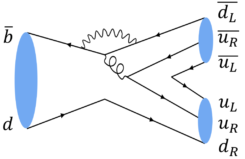
(a) Factorizable penguin

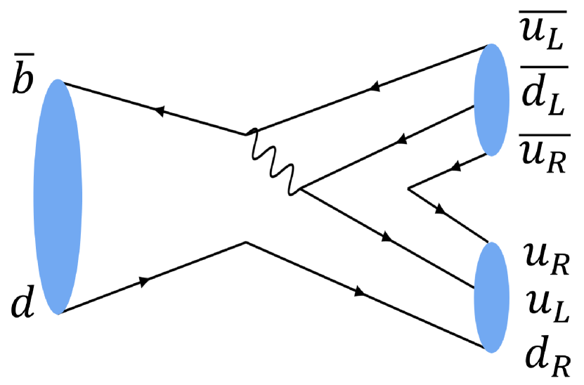
(b) Nonfactorizable tree

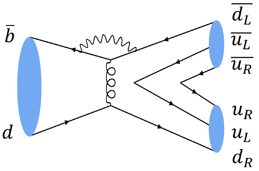
(c) Nonfactorizable penguin

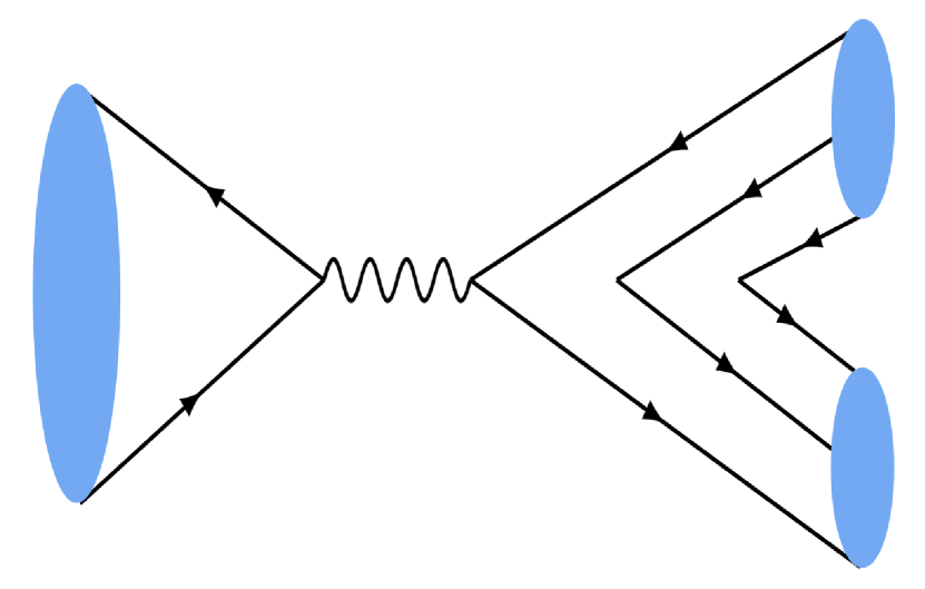
(d) Factorizable tree

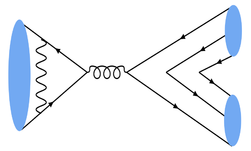
(e) Factorizable tree

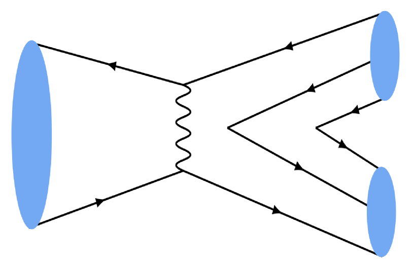
(f) Factorizable penguin

Figure 1: Possible quark line diagrams for $B\to{\bf B}_{n}\overline{\bf B}_{n}^{\prime}$.

Since ${\bf B}_{n}$ and $\overline{\bf B}_{n}^{\prime}$ have the same helicities due to the angular momentum conservation, we have

$$N_{q_{L,R}}=N_{\overline{q}_{R,L}},$$ (6)

in the heavy quark limit, where $N_{q_{L,R}(\overline{q}_{R,L})}$ correspond to the numbers of $q_{L,R}~{}(\overline{q}_{R,L})$ in the (anti)baryons, respectively. The possible spin flavor configurations for $B^{0}\to p\overline{p}$ are shown explicitly in FIGs 1a, 1b and 1c. In contrast, FIGs. 1d, 1e and 1f are not able to fulfill Eq. (6) and therefore suppressed by the chiral symmetry Chua:2003it . One important observation is that FIGs. 1a, 1b and 1c can only be positive helicity. Note that the decay of $B_{s}^{0}\to p\overline{p}$ only receives contributions from FIGs. 1e and 1f and is suppressed consequently, in which the suppression mechanism is similar to $B_{(s)}^{0}\to\mu^{+}\mu^{-}$.

This paper is organized as follows. In Sec. II, we present the formalism. Our numerical results are shown in Sec. III. We conclude the study in Sec. IV.

II formalism

II.1 Factorizable amplitudes

For $\mu\ll M_{W}$ with $\mu$ ($M_{W}$) the energy scale ($W$-boson mass), the charmless weak transition can be described by the effective Hamiltonian, given by Buras:1991jm

$${\cal H}_{eff}=\frac{G_{F}}{\sqrt{2}}\sum_{f=d,s}\left[V_{ub}V_{uf}^{*}\left(C_{1}O^{f}_{1}+C_{2}O^{f}_{2}\right)-V_{tb}V_{tq}^{*}\sum_{i=3}^{10}C_{i}O^{f}_{i}\right]\,+\,h.c.$$ (7)

where $G_{f}$ is the Fermi constant, $V_{ij}$ represent the CKM matrix elements, $q=(u,d,s)$, $C_{1\text{-}10}$ correspond to the Wilson coefficients, and $O_{k}^{f}$ are the operators, defined by

$$\begin{array}[]{ll}O_{1}^{f}=(\overline{u}_{\alpha}\gamma^{\mu}Lb_{\alpha})(\overline{f}_{\beta}\gamma_{\mu}Lu_{\beta})\,,&O_{2}^{f}=(\overline{u}_{\alpha}\gamma^{\mu}Lb_{\beta})(\overline{f}_{\beta}\gamma_{\mu}Lu_{\alpha})\,,\\ O_{3}^{f}=(\overline{f}_{\alpha}\gamma^{\mu}Lb_{\alpha})\sum_{q}(\overline{q}_{\beta}\gamma_{\mu}Lq_{\beta})\,,&O_{4}^{f}=(\overline{f}_{\alpha}\gamma^{\mu}Lb_{\beta})\sum_{q}(\overline{q}_{\beta}\gamma_{\mu}Lq_{\alpha})\,,\\ O_{5}^{f}=(\overline{f}_{\alpha}\gamma^{\mu}Lb_{\alpha})\sum_{q}(\overline{q}_{\beta}\gamma_{\mu}Rq_{\beta})\,,&O_{6}^{f}=(\overline{f}_{\alpha}\gamma^{\mu}Lb_{\beta})\sum_{q}(\overline{q}_{\beta}\gamma_{\mu}Rq_{\alpha})\,,\\ O_{7}^{f}=\frac{3}{2}(\overline{f}_{\alpha}\gamma^{\mu}Lb_{\alpha})\sum_{q}e_{q}(\overline{q}_{\beta}\gamma_{\mu}Rq_{\beta})\,,&O_{8}^{f}=\frac{3}{2}(\overline{f}_{\alpha}\gamma^{\mu}Lb_{\beta})\sum_{q}e_{q}(\overline{q}_{\beta}\gamma_{\mu}Rq_{\alpha})\,,\\ O_{9}^{f}=\frac{3}{2}(\overline{f}_{\alpha}\gamma^{\mu}Lb_{\alpha})\sum_{q}e_{q}(\overline{q}_{\beta}\gamma_{\mu}Lq_{\beta})\,,&O_{10}^{f}=\frac{3}{2}(\overline{f}_{\alpha}\gamma^{\mu}Lb_{\beta})\sum_{q}e_{q}(\overline{q}_{\beta}\gamma_{\mu}Lq_{\alpha})\,,\end{array}$$ (8)

with $f=(d,s)$, $L(R)=1\mp\gamma_{5}$, and the subscripts of $\alpha$ and $\beta$ being the color indexes. Here, $O_{1,2}$ are the tree-level operators, while $O_{3\text{-}6}$ $(O_{7\text{-}10})$ are the (electro-)penguin ones. The amplitudes are then given by sandwiching ${\cal H}_{eff}$ with the initial and final states.

As $C_{7\text{-}10}$ are suppressed due to the smallness of the fine structure constant ($\alpha\approx 1/137$), we would ignore their contributions in this work. Under the factorization framework, the amplitudes of $B\to{\bf B}_{n}\overline{\bf B}_{n}^{\prime}$ can be split into two parts, described by the annihilations of the $B$ mesons and the productions of ${\bf B}_{n}\overline{\bf B}_{n}^{\prime}$ from the vacuum. Symbolically, they are given by

$$\frac{G_{F}}{\sqrt{2}}{\cal C}\langle{\bf B}_{n}\overline{\bf B}_{n}^{\prime}|\overline{q}\Gamma_{\bf B}q^{\prime}|0\rangle\langle 0|\overline{b}\Gamma_{B}q_{B}|B\rangle\,,$$ (9)

where $q_{B}=u,d,s$ for $B=B^{+},B^{0},B_{s}^{0}$, respectively, ${\cal C}$ are related to the CKM matrix elements and Wilson coefficients, and $\Gamma_{{\bf B},B}$ correspond to the Dirac gamma matrices. Accordingly, it is straightforward to see that FIGs. 1a, 1d, 1e and 1f are factorizable, in which the $B$ mesons are annihilated by $O_{1\text{-}6}$. Explicitly, the amplitudes for FIG. 1a are given as

$$A_{a}=\frac{G_{F}}{\sqrt{2}}V_{tb}^{*}V_{tf}f_{B}\left(c_{6}+c_{5}/3\right)\frac{2m_{B}^{2}}{m_{b}}\langle{\bf B}_{n}\overline{\bf B}_{n}^{\prime}|\overline{f}Rq_{B}|0\rangle\,,$$ (10)

where $m_{B(b)}$ are the masses of $B(b)$, and $f_{B}$ are the $B$ meson decay constants. Note that, due to the the charge conservation, only FIG. 1d contributes to the $B^{+}$ decays, given by

$$A_{d}=\frac{G_{F}}{\sqrt{2}}V_{ub}V_{uf}^{*}f_{B^{+}}(c_{1}+c_{2}/3)\left[m_{u}\langle{\bf B}_{n}\overline{\bf B}_{n}^{\prime}|\overline{f}Ru|0\rangle-m_{f}\langle{\bf B}_{n}\overline{\bf B}_{n}^{\prime}|\overline{f}Lu|0\rangle\right]\,,$$ (11)

while the $B^{0}_{(s)}$ decays receive both contributions from FIGs. 1e and 1f, given by

$$A_{e}=\frac{G_{F}}{\sqrt{2}}V_{ub}V_{uf}^{*}f_{B^{0}_{(s)}}(c_{2}+c_{1}/3)2m_{u}\langle{\bf B}_{n}\overline{\bf B}_{n}^{\prime}|\overline{u}\gamma_{5}u|0\rangle\,,$$

$$A_{f}=-\frac{G_{F}}{\sqrt{2}}V_{tb}V_{tf}^{*}f_{B^{0}_{(s)}}[(c_{3}-c_{5})+(c_{4}-c_{6})/3]\sum_{q}2m_{q}\langle{\bf B}_{n}\overline{\bf B}_{n}^{\prime}|\overline{q}\gamma_{5}q|0\rangle\,.$$ (12)

Here, to simplify the formalism, we have used the quark mass hierarchies of $m_{b}\gg m_{s,u,d}$ and the equations of motions,

$$q^{\mu}\langle{\bf B}_{n}\overline{\bf B}_{n}^{\prime}|\overline{q}\gamma_{\mu}q^{\prime}|0\rangle=(m_{q^{\prime}}-m_{q})\langle{\bf B}_{n}\overline{\bf B}_{n}^{\prime}|\overline{q}q^{\prime}|0\rangle\,,$$

$$q^{\mu}\langle{\bf B}_{n}\overline{\bf B}_{n}^{\prime}|\overline{q}\gamma_{\mu}\gamma_{5}q^{\prime}|0\rangle=(-m_{q}-m_{\overline{q}^{\prime}})\langle{\bf B}_{n}\overline{\bf B}_{n}^{\prime}|\overline{q}^{\prime}\gamma_{5}q|0\rangle\,$$ (13)

and

$$\langle 0|\overline{q}\gamma_{5}b|B\rangle=\frac{-im_{B}^{2}}{m_{b}+m_{q}}f_{B}\,,$$ (14)

with $q^{\mu}=p_{{\bf B}_{n}}^{\mu}+p_{\overline{\bf B}_{n}^{\prime}}^{\mu}$. By comparing the amplitudes, we see that $A_{d,e,f}/A_{a}={\cal O}(m_{q}/m_{b})$, which vanish in the heavy quark limit. This result in the factorization approach is consistent with that in the chiral analysis, i.e. $A_{d,e,f}$ can be neglected compared with $A_{a}$.

In the factorization framework, the perturbative effects are taken into account by the Wilson coefficients, while the non-perturbative ones are absorbed into $f_{B}$ and $\langle{\bf B}_{n}\overline{\bf B}_{n}^{\prime}|\overline{q}^{\prime}\Gamma_{\bf B}q|0\rangle$. In this work, the decay constants of $f_{B}$ are given from the evaluations in the lattice QCD Hughes:2017spc . In addition, the baryon productions can be simplified by the merit of the crossing symmetry, given as

$$\langle{\bf B}_{n}(p^{\mu}_{{\bf B}_{n}},S_{{\bf B}_{n}})\overline{\bf B}_{n}^{\prime}(p^{\mu}_{\overline{\bf B}_{n}^{\prime}},S_{\overline{\bf B}_{n}^{\prime}})|\overline{q}\Gamma_{\bf B}q^{\prime}|0\rangle=\langle{\bf B}_{n}(p^{\mu}_{{\bf B}_{n}},S_{{\bf B}_{n}})|\overline{q}\Gamma_{\bf B}q^{\prime}|{\bf B}_{n}^{\prime}(-p^{\mu}_{\overline{\bf B}_{n}^{\prime}},-S_{\overline{\bf B}_{n}^{\prime}})\rangle\,,$$ (15)

where $S$ stands for the spin. Notice that to bring $\overline{\bf B}_{n}^{\prime}$ from the left-handed states to the right-handed ones, we have to take the charge conjugated and flip both the 4-momenta and spins, resulting in that ${\bf B}_{n}^{\prime}$ are unphysical because of the negative energies.

For the ${\bf B}_{n}^{\prime}\to{\bf B}_{n}$ transitions, the scalar and pseudoscalar matrix elements can be parametrized by the form factors, given by

$$\begin{array}[]{c}\langle{\bf B}_{n}|\overline{q}q^{\prime}|{\bf B}_{n}^{\prime}\rangle=\overline{u}_{{\bf B}_{n}}f_{s}(q^{2})u_{{\bf B}_{n}^{\prime}}\,,\\ \langle{\bf B}_{n}|\overline{q}\gamma_{5}q^{\prime}|{\bf B}_{n}^{\prime}\rangle=\overline{u}_{{\bf B}_{n}}g_{a}(q^{2})\gamma_{5}u_{{\bf B}_{n}^{\prime}}\,,\end{array}$$ (16)

where $u$ and $\bar{u}$ represent the Dirac spinors, and $f_{s}(q^{2})$ and $g_{a}(q^{2})$ are the scalar and pseudoscalar form factors, respectively. From the inequality for the on-shell baryons,

$$\left(p_{{\bf B}_{n}}^{\mu}-p_{{\bf B}_{n}^{\prime}}^{\mu}\right)^{2}=q^{2}\leq(m_{{\bf B}_{n}}-m_{\overline{\bf B}_{n}})^{2}\,,$$ (17)

it is clear that the form factors are unphysical at $q^{2}=m_{B}^{2}$.

II.2 Nonfactorizable amplitudes

The nonfactorizable tree diagram for $B^{0}\to p\overline{p}$ is given in FIG. 1b, in which the helicities of $p$ and $\overline{p}$ are found to be positive at the chiral limit. As a result, the quark compositions of the baryon and anti-baryon can be written as $|d_{\uparrow}u_{\downarrow}u_{\uparrow}\rangle$ and $|\overline{u}_{\uparrow}\overline{d}_{\uparrow}\overline{u}_{\downarrow}\rangle$, respectively, where the arrows denote the signs of the helicities. Then, the positive helicity amplitude can be parametrized as

$$A_{b}(B^{0}\to p\overline{p})=\frac{G_{f}}{\sqrt{2}}V_{ub}^{*}V_{ud}C_{T}^{B^{0}\to p\overline{p}}T(B_{0}\to d_{\uparrow}u_{\downarrow}u_{\uparrow},\overline{u}_{\uparrow}\overline{d}_{\uparrow}\overline{u}_{\downarrow}),$$ (18)

with

$$C_{T}^{B^{0}\to p\overline{p}}=6\langle p_{\uparrow}|d_{\uparrow}u_{\downarrow}u_{\uparrow}\rangle 6\langle\overline{p}_{\uparrow}|\overline{u}_{\uparrow}\overline{d}_{\uparrow}\overline{u}_{\downarrow}\rangle\,,$$ (19)

where $T$ stands for the tree contribution to the amplitude at the quark-level in FIG. 1b, $C_{T}$ is the overlapping coefficient between the quarks and baryons, and $|p_{\uparrow}\rangle$ denotes the proton wave function given in Eq. (A). In Eq. (19), the two factors of “6” come from that the low-lying octet baryons are symmetric in the flavor and spin indices.

To relate $A_{b}(B^{0}\to p\overline{p})$ with the others, we utilize the $SU(3)_{F}$ flavor symmetry. It can be done systematically by the following rules with $C_{T}$ being modified accordingly:

• $T$ would remain the same if we replace the quark line of $u$ at the bottom of FIG. 1b with either $d$ or $s$.

• After substituting $B^{+}$ or $B_{s}^{0}$ for $B^{0}$, $T$ is unaltered by modifying the quark constitute of $q_{B}$ in B.

• For $A_{b}(\overline{b}\to\overline{s})$, we replace $\overline{d}_{\uparrow}(V_{ud})$ by $\overline{s}_{\uparrow}(V_{us})$ in the right-handed side of Eq. (18).

In all, for the quark-level amplitudes, we have

$$T(B_{0}\to d_{\uparrow}u_{\downarrow}u_{\uparrow},\overline{u}_{\uparrow}\overline{d}_{\uparrow}\overline{u}_{\downarrow})=T(B\to q_{B\uparrow}u_{\downarrow}q_{\uparrow},\overline{u}_{\uparrow}\overline{f}_{\uparrow}\overline{q}_{\downarrow}).$$ (20)

Consequently, $A(\overline{b}\to\overline{f})$ can be generally parameterized as

$$A_{b}(B\to{\bf B}_{n}\overline{\bf B}_{n})=\frac{G_{f}}{\sqrt{2}}V_{ub}^{*}V_{uf}C_{T}^{B\to{\bf B}_{n}\overline{\bf B}_{n}}T,$$ (21)

with

$$C_{T}^{B\to{\bf B}_{n}\overline{\bf B}_{n}}=36\sum_{q}\langle{\bf B}_{n\uparrow}|q_{B\uparrow}u_{\downarrow}q_{\uparrow}\rangle\langle\overline{\bf B}_{n\uparrow}|\overline{u}_{\uparrow}\overline{f}_{\uparrow}\overline{q}_{\downarrow}\rangle\,.$$ (22)

Similarly, for $A_{c}(\overline{b}\to\overline{f})$, we have

$$A_{c}(B\to{\bf B}_{n}\overline{\bf B}_{n})=-\frac{G_{f}}{\sqrt{2}}V_{tb}^{*}V_{tf}C_{P}^{B\to{\bf B}_{n}\overline{\bf B}_{n}}P$$ (23)

with

$$C_{P}^{B\to{\bf B}_{n}\overline{\bf B}_{n}}=36\sum_{q,q^{\prime}}\langle{\bf B}_{n\uparrow}|q_{B\uparrow}q_{\downarrow}q^{\prime}_{\uparrow}\rangle\langle\overline{\bf B}_{n\uparrow}|\overline{f}_{\uparrow}\overline{q}_{\uparrow}\overline{q}^{\prime}_{\downarrow}\rangle\,,$$ (24)

where $P$ represents the penguin contribution of FIG. 1c.

III Numerical results

To calculate the form factors in Eq. (16), the baryon wave functions are needed. In the framework of the bag model, the quarks are assumed to be confined in a static bag within which the quarks move freely due to the asymptotic freedom. The only free parameter is the bag radius, which can be determined by the mass spectra. Due to its simplicity, it has been widely applied to the baryon decays. However, a static bag is not invariant under the space transition, and hence it could not be an eigenstate of the 4-momentum. Such drawback makes the form factors can only be calculated at $\vec{q}=0$. On the other hand, the modified QCD bag model shown in Ref. Geng:2020ofy , has tackled the problem with the liner superposition of infinite static bags, resulting in the form factors can be uniquely determined even at $\vec{q}\neq 0$. In particular, the experimental decay branching ratios of $\Lambda_{b}\to pK^{-}/\pi^{-}$ and $\Lambda_{b}\to\Lambda\phi$ can be well explained. For the detailed formalism of the modified bag model, along its applications, please refer to Refs. Geng:2020ofy ; Liu:2021rvt ; Geng:2021sxe .

In the calculation, we use the current quark masses of $m_{u,d,s}$ given in the Particle Data Group pdg , and the bag radius is taken to be $R=(5.0\pm 0.2)$ GeV^-1 Geng:2020ofy ; Liu:2021rvt ; Geng:2021sxe . The uncertainties in the bag radius would be presented as error deviations in the branching ratios. Note that the form factors depend little on the quark mass inputs, and the uncertainties in $m_{u,d,s}$ do not affect the results at the precision we consider in this work.

To obtain the form factors in the unphysical region, we utilize the analytic continuations from the physical ones. To illustrate the calculation, we take the $\Lambda\to p$ transition as an example. The $q^{2}$-dependences are shown in FIG. 2, where the dots are the calculated values in the physical region, and the lines are fitted accordingly, which extend to the unphysical region with the $q^{2}$-dependences

$$f_{s}(q^{2})=\frac{f_{s}(0)}{1+\kappa_{2}q^{2}+\kappa_{4}q^{4}}\,,\quad g_{a}(q^{2})=\frac{g_{a}(0)}{1+\kappa_{2}^{\prime}q^{2}+\kappa_{4}^{\prime}q^{4}}\,,$$ (25)

where $\kappa_{2,4}^{(\prime)}$ are the free parameters to be fitted. The exact values of $f_{s}(q^{2})$ and $g_{a}(q^{2})$ at $q^{2}=m_{B^{+}}^{2}$ are found to be

$$f_{s}(m_{B^{+}}^{2})=(3.9\pm 0.2)\times 10^{-3}\,,\quad g_{a}(m_{B^{+}}^{2})=(4.3\pm 0.2)\times 10^{-3}\,,$$ (26)

respectively. From Eq. (26), it can be shown that both ${\bf B}_{n}$ and $\overline{\bf B}_{n}^{\prime}$ are predominated by the positive helicity states, agreeing with the chiral analysis provided in the previous section. Assuming the nonfactorizable amplitudes are ignorable, the results of the decay branching ratios are given in Table I, where ${\cal B}_{a}$ correspond to the contributions from FIG. 1a only.

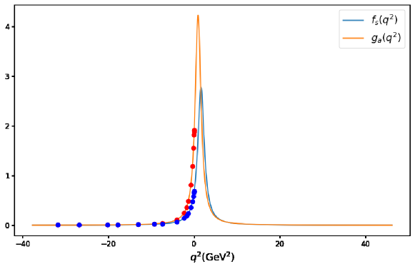
Figure 2: $q^{2}$-dependences of the form factors from the modified bag model, where the results for the dots are calculated directly, while the lines are fitted by the dipole behaviors in Eq. (25).

Particularly, we find that

$$\begin{array}[]{ll}{\cal B}_{a}(B^{+}\to p\overline{\Lambda})=(1.3\pm 0.1)\times 10^{-7}\,,&{\cal B}_{a}(B^{0}\to p\overline{p})=(2\pm 0)\times 10^{-9}\,,\\ {\cal B}_{a}(B^{0}_{s}\to\Xi^{-}\overline{\Xi}^{-})=(28.8\pm 1.5)\times 10^{-7}\,,&{\cal B}_{a}(B^{0}_{s}\to\Xi^{0}\overline{\Xi}^{0})=(27.6\pm 1.5)\times 10^{-7}\,,\\ {\cal B}_{a}(B^{0}\to\Lambda\overline{\Lambda})=(4\pm 0)\times 10^{-9}\,.\end{array}$$ (27)

Our results for the decay branching ratios on $B^{+}\to p\overline{\Lambda}$ and $B^{0}\to p\overline{p}$ are much smaller than the experimental values, showing that the nonfactorizable effects play leading roles, which justify the assumption made in Refs. Chua:2016aqy ; Chua:2013zga . However, in $B_{s}^{0}\to\Xi^{-}\overline{\Xi}^{-}$ and $B_{s}^{0}\to\Xi^{-}\overline{\Xi}^{-}$, the amplitudes of $A_{a}$ contribute significantly, and therefore can not be neglected. On the other hand, ${\cal B}_{a}(B^{0}\to\Lambda\overline{\Lambda})$ is important since it does not receive nonfactorizable contributions as we shall see next.

Note that the matrix elements of $\langle\Sigma|\overline{q}\Gamma_{\bf B}q^{\prime}|\Lambda\rangle$ vanish with $\Sigma=(\Sigma^{\pm},\Sigma^{0})$, so the decays of $B\to(\Sigma\overline{\Lambda},\Lambda\overline{\Sigma})$ do not receive the factorizable contributions. On the other hand, the nonfactorizable amplitudes do contribute in those decays, providing possibilities to explore the nonfactorizable parts. However, it has to be emphasized that the argument would not hold once the $\Sigma^{0}-\Lambda$ mixing are considered Geng:2020tlx , which would cause deviations at $O(10^{-2})$ level.

Table 1: Results for the decay branching ratios, where $C_{T,P}$ are the overlapping coefficients and ${\cal B}~{}({\cal B}_{a})$ corresponds to the (non)factorizable contributions.

$\overline{b}\to\overline{s}$		$C_{T}$	$C_{P}$	$10^{7}{\cal B}_{a}$	$10^{7}{\cal B}$	$\overline{b}\to\overline{d}$		$C_{T}$	$C_{P}$	$10^{8}{\cal B}_{a}$	$10^{8}{\cal B}$
$B^{+}\to$	$p\overline{\Sigma}^{0}$	$-\sqrt{2}$	$\sqrt{2}$	$0.6\pm 0.0$	$0.6\pm 0.1$	$B^{+}\to$	$p\overline{n}$	$-2$	$-10$	$0.2\pm 0.0$	$1.8\pm 0.6$
	$p\overline{\Lambda}$	$-\sqrt{6}$	$-3\sqrt{6}$	$1.3\pm 0.1$	$2.4\pm 0.9$		$\Sigma^{+}\overline{\Sigma}^{0}$	$-2\sqrt{2}$	$-4\sqrt{2}$	$2.9\pm 0.2$	$4.6\pm 0.8$
	$n\overline{\Sigma}^{-}$	$0$	$-2$	$1.1\pm 0.1$	$0.9\pm 0.2$		$\Sigma^{+}\overline{\Lambda}$	$0$	$2\sqrt{6}$	$0$	$0.1\pm 0.1$
	$\Sigma^{+}\overline{\Xi}^{0}$	$-2$	$-10$	$5.0\pm 0.3$	$7.7\pm 2.3$		$\Sigma^{0}\overline{\Sigma}^{-}$	$0$	$4\sqrt{2}$	$2.9\pm 0.2$	$2.2\pm 0.5$
	$\Sigma^{0}\overline{\Xi}^{-}$	$0$	$5\sqrt{2}$	$2.6\pm 0.1$	$1.5\pm 0.7$		$\Xi^{0}\overline{\Xi}^{-}$	$0$	$-2$	$3.5\pm 0.2$	$3.3\pm 0.3$
	$\Lambda\overline{\Xi}^{-}$	$0$	$\sqrt{6}$	$5.7\pm 0.3$	$6.3\pm 0.6$		$\Lambda\overline{\Sigma}^{-}$	$0$	$2\sqrt{6}$	$0$	$0.1\pm 0.1$
$B^{0}\to$	$p\overline{\Sigma}^{+}$	$-2$	$-2$	$1.0\pm 0.1$	$0.8\pm 0.2$	$B^{0}\to$	$p\overline{p}$	$2$	$2$	$0.2\pm 0.0$	$1.2\pm 0.3$
	$n\overline{\Sigma}^{0}$	$-2\sqrt{2}$	$-\sqrt{2}$	$0.5\pm 0.0$	$0.7\pm 0.1$		$n\overline{n}$	$-4$	$-8$	$0.7\pm 0.0$	$5.6\pm 1.4$
	$n\overline{\Lambda}$	$-2\sqrt{6}$	$-3\sqrt{6}$	$1.2\pm 0.1$	$2.4\pm 0.9$		$\Sigma^{0}\overline{\Sigma}^{0}$	$-2$	$-4$	$1.3\pm 0.1$	$2.7\pm 0.4$
	$\Sigma^{0}\overline{\Xi}^{0}$	$-\sqrt{2}$	$-5\sqrt{2}$	$2.3\pm 0.1$	$1.3\pm 0.6$		$\Sigma^{0}\overline{\Lambda}$	$0$	$2\sqrt{3}$	$0$	$0.04\pm 0.04$
	$\Sigma^{-}\overline{\Xi}^{-}$	$0$	$-10$	$4.7\pm 0.3$	$7.1\pm 2.1$		$\Sigma^{-}\overline{\Sigma}^{-}$	$0$	$-8$	$5.3\pm 0.3$	$6.6\pm 1.1$
	$\Lambda\overline{\Xi}^{0}$	$\sqrt{6}$	$\sqrt{6}$	$5.2\pm 0.3$	$5.9\pm 0.5$		$\Lambda\overline{\Sigma}^{0}$	$2\sqrt{3}$	$2\sqrt{3}$	$0$	$3.2\pm 0.9$
							$\Xi^{-}\overline{\Xi}^{-}$	$0$	$2$	$1.6\pm 0.0$	$1.3\pm 0.1$
							$\Lambda\overline{\Lambda}$	$0$	$0$	$0.4\pm 0.0$	$0.4\pm 0.0$
							$\Xi^{0}\overline{\Xi}^{0}$	$0$	$0$	$0$	$<10^{-3}$
							$\Sigma^{+}\overline{\Sigma}^{+}$	$0$	$0$	$0$	$<10^{-3}$
$B_{s}^{0}\to$	$\Sigma^{+}\overline{\Sigma}^{+}$	$2$	$2$	$2.9\pm 0.2$	$2.5\pm 0.3$	$B_{s}^{0}\to$	$\Sigma^{+}\overline{p}$	$-2$	$-2$	$0.4\pm 0.0$	$1.5\pm 0.3$
	$\Sigma^{0}\overline{\Sigma}^{0}$	$1$	$2$	$2.9\pm 0.2$	$2.5\pm 0.3$		$\Sigma^{0}\overline{n}$	$\sqrt{2}$	$-\sqrt{2}$	$0.2\pm 0.0$	$0.8\pm 0.2$
	$\Sigma^{0}\overline{\Lambda}$	$\sqrt{3}$	$0$	$0$	$(5\pm 1)10^{-3}$		$\Xi^{0}\overline{\Sigma}^{0}$	$-4\sqrt{2}$	$-5\sqrt{2}$	$1.0\pm 0.1$	$9.2\pm 2.5$
	$\Sigma^{-}\overline{\Sigma}^{-}$	$0$	$2$	$2.9\pm 0.2$	$2.5\pm 0.3$		$\Xi^{0}\overline{\Lambda}$	$0$	$\sqrt{6}$	$2.2\pm 0.1$	$2.4\pm 0.2$
	$\Xi^{0}\overline{\Xi}^{0}$	$-4$	$-8$	$27.6\pm 1.5$	$32.5\pm 3.7$		$\Xi^{-}\overline{\Sigma^{-}}$	$0$	$-10$	$2.0\pm 0.1$	$3.1\pm 0.9$
	$\Xi^{-}\overline{\Xi}^{-}$	$0$	$-8$	$28.8\pm 1.5$	$33.1\pm 3.8$		$\Lambda\overline{n}$	$-\sqrt{6}$	$-3\sqrt{6}$	$0.5\pm 0.0$	$2.5\pm 0.6$
	$\Lambda\overline{\Sigma}^{0}$	$-\sqrt{3}$	$0$	$0$	$(5\pm 1)10^{-3}$
	$\Lambda\overline{\Lambda}$	$-3$	$-6$	$1.6\pm 0.1$	$2.6\pm 0.8$
	$p\overline{p}$	$0$	$0$	$0$	$<10^{-3}$
	$n\overline{n}$	$0$	$0$	$0$	$<10^{-3}$

Since the nonfactorizable effects in $T$ and $P$ could not be reliably calculated, we may extract their values with the measured branching ratios in Eq. (I). Explicitly, we obtain that

$$T=\left(6.4\pm 1.1\right)10^{-3}\text{GeV}^{3}\,,~{}~{}~{}~{}~{}~{}~{}~{}P=\left(1.7\pm 0.2\right)10^{-4}\text{GeV}^{3},$$ (28)

where the uncertainties come from the experimental input. To reduce the number of the free parameters, we approximate the strong phases in $T$ and $P$ to be zero. A direct consequence is that the CP violating effects are not expected, since the interference from the strong phases is lacking. It is a good approximation for the decays associated with the $\overline{b}\to\overline{d}$ transition, since these decays are dominated by the tree diagram, whereas the relative phase would not be important. On the other hand, for those with the $\overline{b}\to\overline{s}$ transition, by imposing reasonable bounds on the strong phases, the errors on the decay branching ratios are bounded by $1/3$ as shown in Appendix B, which is an acceptable range for the branching ratios as the detail of the QCD dynamic is not well understood yet. However, the resulting CP asymmetries would be huge. For the further discussions on the effects of the strong phases and the direct CP asymmetries, please refer to Ref. Chua:2016aqy . From Eq. (28), the predicted decay branching ratios are given in Table I, labeled as ${\cal B}$.

By taking account of the CKM matrix elements, we find that the decays associated with $\overline{b}\to\overline{s}$ and $\overline{b}\to\overline{d}$ are predominated by $A_{c}$ and $A_{b}$, respectively, which are consistent with the results in Ref. Chua:2016aqy . Accordingly, for the $B^{+}$ decays with the $\overline{b}\to\overline{d}$ transition, only the final states of $p\overline{n}$ and $\Sigma^{+}\overline{\Sigma}^{0}$ receive $A_{b}$ ($C_{T}\neq 0$), and are systematically larger than the others, being good candidates to be measured in the future. Similarly, $B^{0}\to n\overline{n}$ and $B^{0}_{s}\to\Xi^{0}\overline{\Sigma^{0}}$ have the largest values of $C_{T}$, resulting in the largest decay branching ratios, in the $B^{0}$ and $B^{0}_{s}$ decays, respectively.

Likewise, the sizable decay branching ratios with the $\overline{b}\to\overline{s}$ transitions, dominated by the penguin diagrams, are found to be

$${\cal B}(B^{+}\to\Sigma^{+}\overline{\Xi^{0}})=(7.7\pm 2.3)\times 10^{-7}\,,\quad{\cal B}(B^{0}\to\Sigma^{-}\overline{\Xi^{-}})=(7.1\pm 2.1)\times 10^{-7}\,,$$

$${\cal B}(B_{s}^{0}\to\Xi^{0}\overline{\Xi}^{0})=(32.5\pm 3.7)\times 10^{-7}\,,\quad{\cal B}(B_{s}^{0}\to\Xi^{-}\overline{\Xi}^{-})=(33.1\pm 3.8)\times 10^{-7}\,.$$ (29)

In addition, these large values are mainly attributed by $A_{a}$, which can be calculated without the experimental input, making them more promising to be observed in the future experiments. On the other hand, ${\cal B}(B^{0}_{s}\to\Sigma^{0}\overline{\Lambda},\overline{\Sigma}^{0}\Lambda)$ are found to be suppressed since they do not receive contributions from the penguin diagrams.

It is interesting to see that the decays of $B^{0}\to(\Xi^{0}\overline{\Xi}^{0},\Sigma^{+}\overline{\Sigma}^{+})$ and $B^{0}_{s}\to(p\overline{p},n\overline{n})$ are totally factorizable and suffer the helicity suppressions. The suppression mechanism is the same as the one in $B_{(s)}^{0}\to\mu^{+}\mu^{-}$ as emphasized early, and a sizable decay width in the future experiments would be a signal of new physics.

Table 2: Our results comparing with those the literature, the data are taken from the Particle Data Group pdg , while Refs. Hsiao:2014zza and Chua:2016aqy only consider the facotrizable and nonfactorizable amplitudes, respectively.

$10^{8}{\cal B}(B\to{\bf B}_{n}\overline{\bf B}_{n}^{\prime})$	data pdg ; LHCb:2016nbc ; LHCb:2017swz	ours	Ref. Hsiao:2014zza	Ref. Chua:2016aqy
$B^{0}\to p\overline{p}$	$1.25\pm 0.27\pm 0.18$	$1.2\pm 0.3$	$1.4\pm 0.5$	$1.47^{+0.71}_{-0.53}\,{}^{+0.14}_{-0}\,{}^{+2.07}_{-1.16}\pm 0.12$
$B^{+}\to p\overline{\Lambda}$	$24^{+10}_{-8}\pm 3$	$24\pm 9$	$3.5^{+0.7}_{-0.5}\$	$24^{+10.44}_{-8.54}\,{}^{+2.13}_{-0}\,{}^{+12.48}_{-9.85}\pm 0.02$
$B^{0}\to\Lambda\overline{\Lambda}$	$<32$	$0.4\pm 0.0$	$0.3\pm 0.2$	$0\pm 0\pm 0^{+0.23}_{-0}\,{}^{+0.0005}_{-0}$
$B_{s}^{0}\to p\overline{p}$	$<1.5$	$<0.01$	$3.0^{+1.5}_{-1.2}$	$0\pm 0\pm 0^{+0.007}_{-0}$
$B^{0}\to\Xi^{0}\overline{\Xi}^{0}$	-	$325\pm 37$	-	$24.46_{-8.71~{}-0~{}~{}~{}-12.07-0.74}^{+10.53+3.24+16.28+0.75}$
$B^{0}\to\Xi^{-}\overline{\Xi^{-}}$	-	$331\pm 38$	-	$22.63_{-8.05}^{+10.02}\pm 0_{-11.36-0.71}^{+15.27+0.72}$

In Table II, we select several decay channels to compare our results with the theoretical calculations in the literature Chua:2016aqy ; Hsiao:2014zza as well as the data from the experimental measurements pdg ; LHCb:2016nbc ; LHCb:2017swz . Note that Ref. Hsiao:2014zza is focused only on the factorizable amplitudes, whereas Ref. Chua:2016aqy the nonfactorizable ones. Here, the theoretical studies have all used the experimental branching fraction of $B^{0}\to p\overline{p}$ as an input and are thus well consistent with each other. Nonetheless, ${\cal B}(B^{+}\to\overline{\Lambda}p)$ given in Ref. Hsiao:2014zza is too small in comparison with the data. For ${\cal B}(B^{0}\to\overline{\Lambda}\Lambda)$, our non-zero value agrees with that in Ref. Hsiao:2014zza , but differs from the zero prediction in Ref. Chua:2016aqy . On the other hand, due to the factorizable contributions, our results of ${\cal B}(B_{s}^{0}\to\Xi^{0}\overline{\Xi}^{0},\Xi^{-}\overline{\Xi}^{-})$ are ten times larger than the values in Ref. Chua:2016aqy . In addition, we find that the equations of motions are well consistent with the data, which is opposed to the statement for the unsuitable use of the equations of motions in Ref. Hsiao:2014zza . In particular, the decay branching ratio of $B_{s}^{0}\to p\overline{p}$ is found indeed suppressed by $m_{u,d}^{2}/m_{b}^{2}$ and predicted to be $<10^{-10}$, agreeing well with the experimental upper bound.

IV Conclusions

We have systematically analyzed the charmless two-body decays of $B\to{\bf B}_{n}\overline{\bf B}_{n}^{\prime}$. The factorizable amplitudes have been calculated by the modified bag model along with the crossing symmetry and analytic continuation, while the nonfactorizable contributions have been parametrized by the $SU(3)_{F}$ flavor and chiral symmetry, and fitted with the experimental data. Our results are compatible with the current data, and some of the predicted branching ratios can be tested in the ongoing experiments at LHCb and BELLE-II. Explicitly, we have found that the factorizable parts in $B^{+}\to p\overline{\Lambda}$ and $B^{0}\to p\overline{p}$ can be safely neglected, whereas the factorizable ones in $B_{s}^{0}\to(\Xi^{0}\overline{\Xi}^{0},\Xi^{-}\overline{\Xi}^{-})$ are the main contributions with the sizable decay branching ratios of $(32.5\pm 3.7,33.1\pm 3.8)\times 10^{-7}$, respectively, which are promising to be observed by the experiments. We have also shown that the decays associated with the $\overline{b}\to\overline{s}$ and $\overline{b}\to\overline{d}$ transitions are dominated by the penguin and tree diagrams, respectively. In particular, the decays of $B_{s}^{0}\to(\Lambda\overline{\Sigma}^{0},\Sigma^{0}\overline{\Lambda})$ do not receive the penguin contributions with the suppressed decay branching ratios to be $(5\pm 1)\times 10^{-10}$, which can be regarded as good candidates to test our approach. In addition, we have pointed out that the decays of $B^{0}\to(\Xi^{0}\overline{\Xi}^{0},\Sigma^{+}\overline{\Sigma}^{+})$ and $B^{0}_{s}\to(p\overline{p},n\overline{n})$ are helicity suppressed as $B^{0}_{s}\to\mu^{+}\mu^{-}$. It is clearly interesting to see if the future measurements on these decay modes would also show some anomalous effects as that in $B^{0}_{s}\to\mu^{+}\mu^{-}$.

Appendix A Baryon Wave functions

In this appendix, we give the wave functions of ${\bf B}_{n}$, while those of $\overline{\bf B}_{n}$ can be obtained by taking the charge conjugations.

$$\scriptstyle|p_{\uparrow}\rangle= \scriptstyle\frac{\sqrt{2}}{6}\left(2|d_{\downarrow}u_{\uparrow}u_{\uparrow}\rangle-|d_{\uparrow}u_{\downarrow}u_{\uparrow}\rangle-|d_{\uparrow}u_{\uparrow}u_{\downarrow}\rangle-|u_{\downarrow}d_{\uparrow}u_{\uparrow}\rangle-|u_{\downarrow}u_{\uparrow}d_{\uparrow}\rangle+2|u_{\uparrow}d_{\downarrow}u_{\uparrow}\rangle-|u_{\uparrow}d_{\uparrow}u_{\downarrow}\rangle-|u_{\uparrow}u_{\downarrow}d_{\uparrow}\rangle+2|u_{\uparrow}u_{\uparrow}d_{\downarrow}\rangle\right)$$

$$\scriptstyle|n_{\uparrow}\rangle= \scriptstyle\frac{\sqrt{2}}{6}\left(|d_{\downarrow}d_{\uparrow}u_{\uparrow}\rangle+|d_{\downarrow}u_{\uparrow}d_{\uparrow}\rangle+|d_{\uparrow}d_{\downarrow}u_{\uparrow}\rangle-2|d_{\uparrow}d_{\uparrow}u_{\downarrow}\rangle-2|d_{\uparrow}u_{\downarrow}d_{\uparrow}\rangle+|d_{\uparrow}u_{\uparrow}d_{\downarrow}\rangle-2|u_{\downarrow}d_{\uparrow}d_{\uparrow}\rangle+|u_{\uparrow}d_{\downarrow}d_{\uparrow}\rangle+|u_{\uparrow}d_{\uparrow}d_{\downarrow}\rangle\right)$$

$$\scriptstyle|\Sigma^{+}_{\uparrow}\rangle= \scriptstyle\frac{\sqrt{2}}{6}\left(-2|s_{\downarrow}u_{\uparrow}u_{\uparrow}\rangle+|s_{\uparrow}u_{\downarrow}u_{\uparrow}\rangle+|s_{\uparrow}u_{\uparrow}u_{\downarrow}\rangle+|u_{\downarrow}s_{\uparrow}u_{\uparrow}\rangle+|u_{\downarrow}u_{\uparrow}s_{\uparrow}\rangle-2|u_{\uparrow}s_{\downarrow}u_{\uparrow}\rangle+|u_{\uparrow}s_{\uparrow}u_{\downarrow}\rangle+|u_{\uparrow}u_{\downarrow}s_{\uparrow}\rangle-2|u_{\uparrow}u_{\uparrow}s_{\downarrow}\rangle\right)$$

$$\scriptstyle|\Sigma^{0}_{\uparrow}\rangle= \scriptstyle\frac{1}{6}\left(-|d_{\downarrow}s_{\uparrow}u_{\uparrow}\rangle-|d_{\downarrow}u_{\uparrow}s_{\uparrow}\rangle+2|d_{\uparrow}s_{\downarrow}u_{\uparrow}\rangle-|d_{\uparrow}s_{\uparrow}u_{\downarrow}\rangle-|d_{\uparrow}u_{\downarrow}s_{\uparrow}\rangle+2|d_{\uparrow}u_{\uparrow}s_{\downarrow}\rangle+2|s_{\downarrow}d_{\uparrow}u_{\uparrow}\rangle+2|s_{\downarrow}u_{\uparrow}d_{\uparrow}\rangle-|s_{\uparrow}d_{\downarrow}u_{\uparrow}\rangle-|s_{\uparrow}d_{\uparrow}u_{\downarrow}\rangle\right.$$

$$\scriptstyle\qquad\left.-|s_{\uparrow}u_{\downarrow}d_{\uparrow}\rangle-|s_{\uparrow}u_{\uparrow}d_{\downarrow}\rangle-|u_{\downarrow}d_{\uparrow}s_{\uparrow}\rangle-|u_{\downarrow}s_{\uparrow}d_{\uparrow}\rangle-|u_{\uparrow}d_{\downarrow}s_{\uparrow}\rangle+2|u_{\uparrow}d_{\uparrow}s_{\downarrow}\rangle+2|u_{\uparrow}s_{\downarrow}d_{\uparrow}\rangle-|u_{\uparrow}s_{\uparrow}d_{\downarrow}\rangle\right)$$

$$\scriptstyle|\Sigma^{-}_{\uparrow}\rangle= \scriptstyle\frac{\sqrt{2}}{6}\left(-|d_{\downarrow}d_{\uparrow}s_{\uparrow}\rangle-|d_{\downarrow}s_{\uparrow}d_{\uparrow}\rangle-|d_{\uparrow}d_{\downarrow}s_{\uparrow}\rangle+2|d_{\uparrow}d_{\uparrow}s_{\downarrow}\rangle+2|d_{\uparrow}s_{\downarrow}d_{\uparrow}\rangle-|d_{\uparrow}s_{\uparrow}d_{\downarrow}\rangle+2|s_{\downarrow}d_{\uparrow}d_{\uparrow}\rangle-|s_{\uparrow}d_{\downarrow}d_{\uparrow}\rangle-|s_{\uparrow}d_{\uparrow}d_{\downarrow}\rangle\right)$$

$$\scriptstyle|\Xi^{-}_{\uparrow}\rangle= \scriptstyle\frac{\sqrt{2}}{6}\left(-2|d_{\downarrow}s_{\uparrow}s_{\uparrow}\rangle+|d_{\uparrow}s_{\downarrow}s_{\uparrow}\rangle+|d_{\uparrow}s_{\uparrow}s_{\downarrow}\rangle+|s_{\downarrow}d_{\uparrow}s_{\uparrow}\rangle+|s_{\downarrow}s_{\uparrow}d_{\uparrow}\rangle-2|s_{\uparrow}d_{\downarrow}s_{\uparrow}\rangle+|s_{\uparrow}d_{\uparrow}s_{\downarrow}\rangle+|s_{\uparrow}s_{\downarrow}d_{\uparrow}\rangle-2|s_{\uparrow}s_{\uparrow}d_{\downarrow}\rangle\right)$$

$$\scriptstyle|\Xi^{0}_{\uparrow}\rangle= \scriptstyle\frac{\sqrt{2}}{6}\left(-|s_{\downarrow}s_{\uparrow}u_{\uparrow}\rangle-|s_{\downarrow}u_{\uparrow}s_{\uparrow}\rangle-|s_{\uparrow}s_{\downarrow}u_{\uparrow}\rangle+2|s_{\uparrow}s_{\uparrow}u_{\downarrow}\rangle+2|s_{\uparrow}u_{\downarrow}s_{\uparrow}\rangle-|s_{\uparrow}u_{\uparrow}s_{\downarrow}\rangle+2|u_{\downarrow}s_{\uparrow}s_{\uparrow}\rangle-|u_{\uparrow}s_{\downarrow}s_{\uparrow}\rangle-|u_{\uparrow}s_{\uparrow}s_{\downarrow}\rangle\right)$$

$$\scriptstyle|\Lambda_{\uparrow}\rangle= \scriptstyle\frac{1}{\sqrt{12}}\left(|d_{\downarrow}s_{\uparrow}u_{\uparrow}\rangle+|d_{\downarrow}u_{\uparrow}s_{\uparrow}\rangle-|d_{\uparrow}s_{\uparrow}u_{\downarrow}\rangle-|d_{\uparrow}u_{\downarrow}s_{\uparrow}\rangle+|s_{\uparrow}d_{\downarrow}u_{\uparrow}\rangle-|s_{\uparrow}d_{\uparrow}u_{\downarrow}\rangle-|s_{\uparrow}u_{\downarrow}d_{\uparrow}\rangle+|s_{\uparrow}u_{\uparrow}d_{\downarrow}\rangle\right.$$ (30)

$$\scriptstyle\qquad\left.-|u_{\downarrow}d_{\uparrow}s_{\uparrow}\rangle-|u_{\downarrow}s_{\uparrow}d_{\uparrow}\rangle+|u_{\uparrow}d_{\downarrow}s_{\uparrow}\rangle+|u_{\uparrow}s_{\uparrow}d_{\downarrow}\rangle\right)$$

Appendix B Uncertainties from strong phases

Let $A_{P}$ and $A_{T}$ be the penguin and tree contributions to the amplitude of a particular decay channel, respectively. Without lost of generality, we take $A_{P}$ to be real (possibly negative) and $A_{T}=|A_{T}|e^{i\phi}$ with $\pi/2\geq\phi\geq-\pi/2$ being the phase. The effects on the branching ratios of $\phi$ can be parameterized as

$$\xi\equiv 1-\frac{{\cal B}_{nc}}{{\cal B}}=1-\frac{\left|A_{P}+|A_{T}|\right|^{2}}{|A_{P}+A_{T}|^{2}}\,,$$ (31)

where the subscript of “$nc$” denotes that $\phi$ is taken as zero. In general, it obeys the inequality

$$\frac{2|A_{P}A_{T}|}{A_{P}^{2}+|A_{T}^{2}|}\geq\xi\geq-\frac{2|A_{P}A_{T}|}{A_{P}^{2}+|A_{T}^{2}|}\,,$$ (32)

and

$$1\geq\xi\geq\frac{\cos\phi-1}{1+\cos\phi}\,,$$ (33)

where the equations hold at $\phi=\pm\pi/2$ and $A_{P}=|A_{T}|$, respectively. In reality, we have $A_{T}\gg A_{P}$ for the decays associated with the $\overline{b}\to\overline{d}$ transition, and therefore the strong phases shall affect little in these decays. On the other hand, for those with $\overline{b}\to\overline{s}$, the actual values of $\xi$ are bounded by $1/3$ from Eq. (32), which is within the uncertainties we consider in this work.

In addition, it is reasonable to expect that the strong phases are bounded by $|\phi|\leq\pi/4$ as found in the $B\to VV$ decays with $V=\{\rho(770),\omega(782),K^{*}(892),\phi(1020)\}$ pdg ; Geng:2021lrc . In these cases, the inequality can be further tightened to be

$$\xi\geq 2\sqrt{2}-3\,,$$ (34)

based on Eq. (33),

References

• (1) R. Aaij et al. [LHCb], Phys. Rev. Lett. 118, 191801 (2017).
• (2) R. Aaij et al. [LHCb], [arXiv:2108.09283].
• (3) R. Aaij et al. [LHCb], [arXiv:2108.09284].
• (4) M. Aaboud et al. [ATLAS], JHEP 04, 098 (2019).
• (5) A. M. Sirunyan et al. [CMS], JHEP 04, 188 (2020).
• (6) T. Hermann, M. Misiak and M. Steinhauser, JHEP 12, 097 (2013).
• (7) C. Bobeth, M. Gorbahn, T. Hermann, M. Misiak, E. Stamou and M. Steinhauser, Phys. Rev. Lett. 112, 101801 (2014).
• (8) C. Bobeth, M. Gorbahn and E. Stamou, Phys. Rev. D 89, 034023 (2014).
• (9) M. Beneke, C. Bobeth and R. Szafron, Phys. Rev. Lett. 120, 011801 (2018).
• (10) M. Beneke, C. Bobeth and R. Szafron, JHEP 10, 232 (2019).
• (11) R. Aaij et al. [LHCb], JHEP 04, 162 (2017).
• (12) R. Aaij et al. [LHCb], Phys. Rev. Lett. 119, 232001 (2017).
• (13) P. A. Zyla et al. [Particle Data Group], PTEP 2020, 083C01 (2020).
• (14) N. G. Deshpande, J. Trampetic and A. Soni, Mod. Phys. Lett. A 3, 749 (1988).
• (15) V. L. Chernyak and I. R. Zhitnitsky, Nucl. Phys. B 345, 137 (1990).
• (16) X. G. He, B. H. J. McKellar and D. d. Wu, Phys. Rev. D 41, 2141 (1990).
• (17) S. M. Sheikholeslami and M. P. Khanna, Phys. Rev. D 44, 770 (1991).
• (18) P. Ball and H. G. Dosch, Z. Phys. C 51, 445 (1991).
• (19) M. Jarfi, O. Lazrak, A. Le Yaouanc, L. Oliver, O. Pene and J. C. Raynal, Phys. Rev. D 43, 1599 (1991).
• (20) H. Y. Cheng and K. C. Yang, Phys. Rev. D 66, 014020 (2002).
• (21) C. H. V. Chang and W. S. Hou, Eur. Phys. J. C 23, 691 (2002).
• (22) C. K. Chua, Phys. Rev. D 68, 074001 (2003).
• (23) Z. Luo and J. L. Rosner, Phys. Rev. D 67, 094017 (2003).
• (24) H. Y. Cheng and J. G. Smith, Ann. Rev. Nucl. Part. Sci. 59, 215 (2009).
• (25) H. Y. Cheng and C. K. Chua, Phys. Rev. D 91, 036003 (2015).
• (26) Y. K. Hsiao and C. Q. Geng, Phys. Rev. D 91, 077501 (2015).
• (27) C. K. Chua, Phys. Rev. D 89, 056003 (2014).
• (28) C. K. Chua, Phys. Rev. D 95, 096004 (2017).
• (29) A. J. Buras, M. Jamin, M. E. Lautenbacher and P. H. Weisz, Nucl. Phys. B 370, 69 (1992).
• (30) C. Hughes, C. T. H. Davies and C. J. Monahan, Phys. Rev. D 97, 054509 (2018).
• (31) C. Q. Geng, C. W. Liu and T. H. Tsai, Phys. Rev. D 102, 034033 (2020).
• (32) C. Q. Geng and C. W. Liu, JHEP 11, 104 (2021).
• (33) C. W. Liu and C. Q. Geng, JHEP 01, 128 (2022).
• (34) C. Q. Geng, C. W. Liu and T. H. Tsai, Phys. Rev. D 101, 054005 (2020).
• (35) C. Q. Geng and C. W. Liu, Phys. Lett. B 825, 136883 (2022).