A Linear Relation Between the Color Stretch $s_{BV}$ and the Rising Color Slope $s_{0}^{*}(B-V)$ of Type Ia Supernovae

Abstract

Using data from the Complete Nearby ($z_{\rm host}<0.02$) sample of Type Ia Supernovae (CNIa0.02), we discover a linear relation between two parameters derived from the $B-V$ color curves of Type Ia supernovae: the “color stretch” $s_{BV}$ and the rising color slope $s_{0}^{*}(B-V)$ after the peak, and this relation applies to the full range of $s_{BV}$. The $s_{BV}$ parameter is known to be tightly correlated with the peak luminosity, and especially for “fast decliners” (dim Type Ia supernovae), and the luminosity correlation with $s_{BV}$ is markedly better than with the classic light-curve width parameters such as $\Delta{m_{15}(B)}$. Thus our new linear relation can be used to infer peak luminosity from $s_{0}^{*}$. Unlike $s_{BV}$ (or $\Delta{m_{15}}$), the measurement of $s_{0}^{*}(B-V)$ does not rely on the well-determined time of light-curve peak or color maximum, making it less demanding on the light-curve coverage than past approaches.

1 INTRODUCTION

As a supernova (SN) population, SNe Ia show remarkable regularities in observed properties, and in particular, their light curves follow a tight relation between peak luminosity and the decline rate, which is commonly referred to as the width-luminosity relation (WLR, see Phillips & Burns 2017 for a review). The empirical WLR extends from the most luminous 1991T-like SNe Ia (Filippenko et al., 1992a; Ruiz-Lapuente et al., 1992; Phillips et al., 1992) to the least luminous 1991bg-like SNe Ia (Filippenko et al., 1992b; Leibundgut et al., 1993; Turatto et al., 1996). The WLR not only offers important clues to understanding the physics of the SN Ia population, but also enables using SNe Ia as important cosmological distance indicators.

Pskovskii (1977, 1984) suggested the existence of WLR for SNe Ia by using a post-peak slope parameter, $\beta$, to measure the light-curve decline rate. Its validity was called into question by some researchers due to concerns over host-galaxy contamination to the SN flux measurements obtained with photographic plates (see, e.g., Boisseau & Wheeler, 1991). Phillips (1993) established the WLR by using well-sampled light curves of nearby SNe Ia observed with charge-coupled devices (CCDs) and introduced the now-classic width parameter $\Delta m_{15}(B)$, which is the $B$-band magnitude difference between the peak $t_{\rm peak}(B)$ and 15 days afterwards. Later, other similar width parameterizations such as the “stretch” $s$ were introduced (Perlmutter et al., 1997), and there were also variants like $x_{1}$ in SALT2 (Guy et al., 2007) or $\Delta$ (Jha et al., 2007).

In order to accurately derive $\Delta m_{15}(B)$ directly from the light curve, a good photometric coverage before $t_{\rm peak}(B)$ to at least 15 days after $t_{\rm peak}(B)$ is required. Since the light curves evolve slowly over the peak (varying by only $\sim 0.1$ mag in one week), accurate peak time determination is challenging if the light curve is not densely sampled around the peak. In practice, various template-fitting methods are often employed to derive $\Delta m_{15}(B)$ using well-sampled light-curve templates with known $\Delta m_{15}(B)$ (see, e.g., Hamuy et al., 1995, 1996; Prieto et al., 2006; Burns et al., 2011).

For low-luminosity, fast-declining SNe Ia, $\Delta m_{15}(B)$ is found to be a poor width discriminator, and the WLR using $\Delta m_{15}(B)$ shows a large scatter for $\Delta m_{15}(B)\gtrsim 1.7$ mag (see, e.g., Burns et al., 2014; Gall et al., 2018). Similarly, the stretch method fails for fast decliners (see, e.g., Phillips & Burns, 2017). From studying high-quality $B-V$ color curves of SNe Ia observed by the Carnegie Supernova Project (CSP), Burns et al. (2014) found that fast-declining SNe Ia reach their reddest $B-V$ color earlier than those with slower decline rates. To better characterize this, Burns et al. (2014) introduced the “color stretch” parameter, $s_{BV}$, which is a dimensionless stretch-like parameter defined as $s_{BV}=t_{\rm max}(B-V)/(30~{}{\rm days})$, where $t_{\rm max}(B-V)$ is time to the maximum (reddest) $B-V$ color with reference to the $B$-band maximum. Since the $B-V$ color quickly declines after reaching maximum, $t_{\rm max}(B-V)$ corresponds to a sharp “break” in the $B-V$ color curve (see Fig 1 for examples). Using $s_{BV}$ as a proxy for decline rate (instead of $\Delta m_{15}$), the scatter in WLR significantly reduces at the low-luminosity end, and SNe Ia over the full range of luminosity lie on a tight and continuous correlation (Burns et al., 2018). Moreover, Ashall et al. (2020) found that combining $s_{BV}$ with the time difference between $B$-band and $i$-band maxima is useful to discriminate between SNe Ia subtypes.

Reducing the scatter in WLR using $s_{BV}$ not only has important implications for using SNe Ia as distance indicators, but also sheds new insight into the physics of WLRs. Wygoda et al. (2019) found that $t_{\rm max}(B-V)$ corresponds to an abrupt change in the mean opacities due to ionization-state transitions of ⁵⁶Fe and ⁵⁶Co in the ejecta, while the timescale to reach the color maximum is determined by the ejecta ⁵⁶Ni column density which sets the recombination time of Fe/Co ions.

To derive $s_{BV}$ from light curves, it is required to measure not only $t_{\rm max}(B-V)$, but also, like $\Delta m_{15}$, a precise estimate of $t_{\rm peak}(B)$ is also needed.

In this work, we report the discovery of a linear relation between $s_{BV}$ and the rising linear slope of $B-V$ color curve of SNe Ia, which is defined as $s_{0}^{*}(B-V)$ by us, using the CNIa0.02 sample (Chen et al., 2020). As a proxy for light-curve width and in turn the peak luminosity via WLR, $s_{0}^{*}(B-V)$ has the merit of being less demanding on light curve coverage.

2 Light-curve Analysis

In this work, we analyze the $B$- and $V$-band light curves presented in Chen et al. (2020). We include SNe Ia ranging from the most luminous end (i.e, 1991T-like) to the least luminous end (i.e., 1991bg-like) in the analysis, while we exclude several peculiar Ia-like objects that are known to deviate from the WLR (e.g., Iax-type objects such as SN 2017gbb classified by Lyman et al. 2017 and the 2009dc-like SN Ia-peculiar, ASASSN-15pz studied by Chen et al. 2019). In order to obtain accurate $s_{BV}$ measurements, we need to reliably infer the time of the $B$-band peak , $t_{\rm peak}(B)$, and the time of maximum $B-V$ color, $t_{\rm max}(B-V)$. We discuss below how we select the SNe used in the analysis.

First, the $B$-band light curves need to have coverage around the peak to infer $t_{\rm peak}(B)$. We adopt the criterion of having at least 3 epochs within 6 days of the peak and at least 4 points within 10 days of the peak. $t_{\rm peak}(B)$ is used as the reference time throughout the paper. $t_{\rm peak}(B)$ is obtained with the Gaussian process method if pre-peak data are available, otherwise it is derived from template fitting using SNooPy (Burns et al., 2011). We list the derived $t_{\rm peak}(B)$ and $\Delta m_{15}(B)$ in Table 1.

Then we analyze the $B-V$ color curves for all remaining SNe to infer $s_{BV}$, and the SNe without data late enough to derive $t_{\rm max}(B-V)$ are excluded from the analysis. To obtain reliable $s_{BV}$, we impose the following selection criteria: 1) the $B-V$ color curve needs to have at least 4 data points covering no less than half of the time range between $t_{\rm peak}(B)$ and $t_{\rm max}(B-V)$; 2) after $t_{\rm max}(B-V)$, there need to be at least 2 data points spanning more than 5 days, and the last data point needs to be at least $\sim$ 10 days after $t_{\rm max}(B-V)$. The phase of the $B-V$ color curve is corrected for time dilation. Since all targets have low redshifts, the K-correction is negligible for our analysis and thus is not applied.

In Figure 1, we show the $B-V$ color curves of three SNe with $s_{BV}=0.41,0.90,{\rm and}\,1.11$, respectively. After $t_{\rm peak}(B)$, the $B-V$ color curve soon enters into a linear rise phase (hence, becoming redder) followed by a linear decline (becoming bluer) after $t_{\rm max}(B-V)$. The rising slope and $t_{\rm max}(B-V)$ - $t_{\rm peak}(B)$ seem to correlate with each other, and we measure the relevant light-curve parameters to quantitatively study the observed correlation. In the following, we describe how we measure the parameters from the color curves.

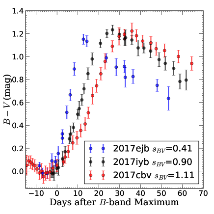
Figure 1: $B-V$ color curves of three SNe: 2017ejb, 2017iyb and 2017cbv. The data of 2017ejb is shifted downwards by 0.25 magnitude to match the local minimum of $B-V$ color, $(B-V)_{\rm min}$, of the other two SNe. After $B$-band peak, the $B-V$ color curves have the typical evolution of first rise and then decline. The three SNe reach their maximum $B-V$ colors at different times which correspond to different $s_{BV}$ values (see text for how they are measured). The rising slope seems to be correlated with the time of the maximum $B-V$ color.

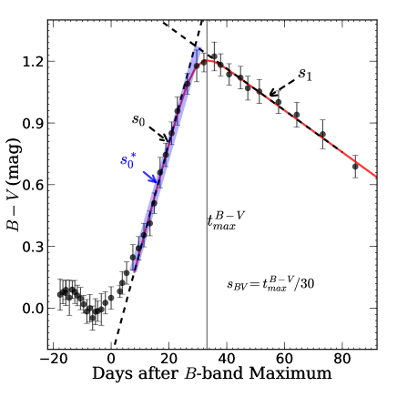
Figure 2: $B-V$ color curve of SN 2017cbv with best-fit results shown as an example of the procedure described in this paper. The observed data are shown as black dots and, the best-fit model with Eq. (1) for the data is shown in red. The black dashed lines indicate the rising slope $s_{0}$ and declining slope $s_{1}$ from Eq. (1). The vertical black line marks the time of reddest $B-V$ color. The direct linear fit of the rising slope to get $s_{0}^{*}(B-V)$ is shown as the blue line.

We fit the time evolution of the $B-V$ color since the onset of the post-peak linear rise phase based on Eq. (2) in Burns et al. (2014). The model has the form

$$y(t)=\frac{1}{2}(s_{0}+s_{1})t+\frac{\tau}{2}(s_{1}-s_{0})\ln[\cosh\left(\frac{t-t_{\rm h}}{\tau}\right)]+c,$$ (1)

where $s_{0}$ and $s_{1}$ characterize the rising and declining slopes, respectively, $\tau$ is the transition time scale indicating how fast the color curve changes from the rising to the declining slope, and $t_{\rm h}$ is the time when the derivative of $y(t)$ equals to the averaged value of the initial and final slopes, i.e, $y^{\prime}(t_{\rm h})={(s_{0}+s_{1})}{/2}$. We drop the last polynomial term on the right-hand side in Eq. (2) of Burns et al. (2014), and that term is used for modeling the color curve prior to the onset of the linear rise phase. In addition, we also correct a typographical error in the first term (correcting ${(s_{0}-s_{1})}/{2}$ in Burns et al. (2014) to $(s_{0}+s_{1})t/2$). Note that, in this model, the rising and declining sides are not strictly linear with time, and $s_{0}$ and $s_{1}$ are only supposed to be close to the first derivatives for most parts of the two sides, respectively. We show an example of SN 2017cbv in Figure 2, in which the best-fit model is shown as a red line. The time of the maximum $B-V$ color where $y^{\prime}(t_{\rm max}(B-V))=0$, as indicated by the vertical line in Figure 2, is

$$t_{\rm max}(B-V)=\frac{\tau}{2}\ln\left(-\frac{s_{0}}{s_{1}}\right)+t_{\rm h}$$ (2)

We note that the phase when the linear rise starts, $t_{s}$, is correlated with $t_{\rm max}(B-V)$. We adopt an empirical estimate of $t_{s}=0.3t_{\rm max}(B-V)-2$ days after $t_{\rm peak}(B)$ as the start phase for our fitting. The adopted end phase for fitting is 90 days after $t_{\rm peak}(B)$. Since $t_{\rm max}(B-V)$ is needed to derive the phase range used for the fit, we iteratively determine this phase range with an initial range of [5, 90] days.

We fit the $B-V$ color curves using the Markov chain Monte Carlo (MCMC) method with uniform priors for all parameters. Eq. (2) is used to determine $t_{\rm max}(B-V)$ and then $s_{BV}=t_{\rm max}(B-V)/30$. The derived $s_{BV}$, $s_{0}$ and $s_{1}$ parameters for 87 SNe Ia with their uncertainties are given in Table 1.

Our work was initially motivated by the apparent correlation between $s_{BV}$ and $s_{0}$. However, upon further investigations, we find that the value of $s_{0}$ derived from Eq. (1) depends on the prior placed on the transition timescale $\tau$. The reason for this dependence can be understood by examining the time derivative of Eq. (1),

$$y^{\prime}(t)=\frac{s_{0}+s_{1}}{2}+\frac{s_{1}-s_{0}}{2}\tanh\left(\frac{t-t_{h}}{\tau}\right).$$ (3)

Clearly the deviation of $y^{\prime}(t)$ from a constant (i.e., as followed from a linear model with respect to $t$) in the rising part of the model depends on $\tau$. In practice, the derived values of $\tau$ often have relatively large uncertainties, and they also correlate with $s_{BV}$, making it difficult to establish a clearcut correlation between $s_{0}$ and $s_{BV}$.

Instead of using $s_{0}$ defined in Eq. (1), we measure the rising slope by directly fitting a linear model $y(t)=s_{0}^{*}\times t+c^{*}$ to the rising part of the color curve. To do so, we need to determine a phase range [$t_{s}$, $t_{e}$] during which the color curve is well-characterized by a linear model. As can be seen from Figure 1, both the beginning and the end phases of the linear phase seem to be correlated with the time of maximum $B-V$ color. Therefore, the values of $t_{s}$ and $t_{e}$ depend on $t_{\rm max}(B-V)$. After some experimentations, we find that the range defined with $t_{s}=0.3t_{\rm max}(B-V)-2$ and $t_{e}=0.9t_{\rm max}(B-V)$ can be well characterized by a linear model for SNe with a broad range of $s_{BV}$. The best-fit linear model within such a range is shown as a blue line in Figure 2. We exclude SNe with less than 3 points on the $B-V$ color curve within [$t_{s}$, $t_{e}$] from the analysis. The directly measured rising color slope parameters, $s_{0}^{*}$, are provided in Table 1. By comparing the values of $s_{0}$ and $s_{0}^{*}$, we find that $s_{0}$ tends to be larger than $s_{0}^{*}$.

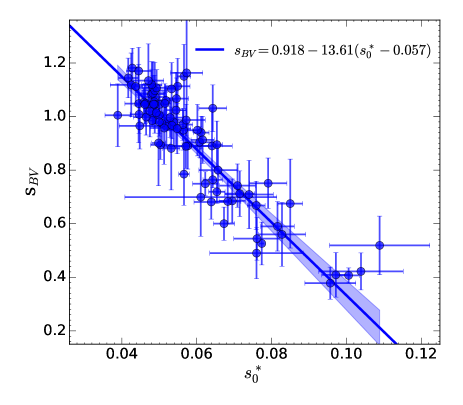
Figure 3: Correlation between the color-stretch parameter, s_BV, and the rising color slope, $s_{0}^{*}$, of the $B-V$ color. All the measurements for 87 SNe in Table 1 are shown here. The blue line is the best linear fit and the shaded range indicates the 95% confidence region for the fit.

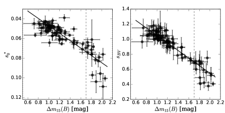
Figure 4: Comparisons of $s_{0}^{*}(B-V)$ (left) and $s_{BV}$ (right) with respect to $\Delta{m_{15}(B)}$, respectively. For SNe with $m_{15}(B)<1.7$ (vertical dashed lines), both $s_{0}^{*}$ and $s_{BV}$ are linearly correlated with $\Delta{m_{15}(B)}$ (the black lines in both panels), whereas there is a large scatter for fast decliners with $m_{15}(B)>1.7$.

3 Results

As shown in Figure 3, we discover that $s_{0}^{*}$ and $s_{BV}$ are linearly correlated, and the linear correlation coefficient is $r=-0.90$, which is highly significant. The best-fit linear model between $s_{0}^{*}$ and $s_{BV}$ accounting for uncertainties yields

$$s_{BV}=0.918(0.008)-13.61(0.61)\times(s_{0}^{*}-0.057).$$ (4)

The uncertainties given in the parentheses are obtained by scaling the measurement errors of $s_{0}^{*}$ and $s_{BV}$ to have $\chi^{2}/dof=1$. The residuals to this best-fit linear model have a scatter of 0.093 in $s_{BV}$, which is comparable with the median $s_{BV}$ measurement uncertainty of 0.082. The uncertainties in the $s_{0}^{*}$ inference also affect how tight the derived relation is. This linear relation between $s_{BV}$ and $s_{0}^{*}$ suggests that $s_{0}^{*}$ can be used to infer $s_{BV}$.

As shown in the left panel of Fig. 4, we compare $s_{0}^{*}(B-V)$ with $\Delta m_{15}(B)$ using our sample. Similar to the well-known trends (Burns et al., 2014) when comparing $s_{BV}$ and $\Delta m_{15}(B)$ (right panel of Fig. 4), there is a linear correlation for SNe with $\Delta m_{15}(B)<1.7$, but for those with $\Delta m_{15}(B)>1.7$, there is a large scatter.

The inference of $s_{0}^{*}$ has the comparative merit over $s_{BV}$ or $\Delta m_{15}(B)$ on the data coverage requirements. Measuring $s_{BV}$ depends on determining two critical timing parameters, $t_{\rm peak}(B)$ and $t_{\rm max}(B-V)$. The measurement of $\Delta m_{15}(B)$ is also highly sensitive to how well $t_{\rm peak}(B)$ is determined. In comparison, deriving $s_{0}^{*}$ is simply measuring a slope, which does not require determining either of those two timings, and instead, $s_{0}^{*}$ can be determined for a SN which is not observed around the peak and/or lacks the coverage at later times around $t_{\rm max}(B-V)$.

4 Measurement Procedure

In practice, when either $t_{\rm peak}(B)$ or $t_{\rm max}(B-V)$ is absent, it is not possible to use the phase range of ([$t_{s}=0.3t_{\rm max}(B-V)-2$, $t_{e}=0.9t_{\rm max}(B-V)$]) with respect to $t_{\rm peak}(B)$ to fit $s_{0}^{*}$. Below we provide a practical procedure to measure $s_{0}^{*}$ for such light curves:

• If the $B$-band light curve around the peak is available to measure $t_{\rm peak}(B)$, but there is no sufficiently late observation to determine the break time in the $B-V$ color curve. First, start with fitting all data after $t_{\rm peak}(B)$ to get the initial $s_{0}^{*}$, and then use Eq. (4) to estimate $s_{BV}$ and subsequently $t_{\rm max}(B-V)=s_{BV}\times 30\,{\rm d}$. Then use the range of [$0.3t_{\rm max}(B-V)-2$, $0.9t_{\rm max}(B-V)$] for the next fitting and iteratively repeat this process until it converges.

• If the $B-V$ color curve around the break time is available to measure the time of maximum $B-V$ color, but there is no $B$-band coverage over the peak to measure $t_{\rm peak}(B)$. In this case without the reference time of $t_{\rm peak}(B)$, a new reference time of $t_{\rm break}$ (measured as the time of maximum $B-V$ color) will be used. First, start with fitting all data before t_break to get the initial $s_{0}^{*}$ and then use Eq. (4) to estimate $t_{\rm max}(B-V)$. Then use the range from $0.7t_{\rm max}(B-V)+2$ to $0.1t_{\rm max}(B-V)$ days before $t_{\rm break}$ for the next fitting and iteratively repeat this process until it converges.

• If neither the $B$-band peak nor the break part in the $B-V$ color curve is available. The $s_{0}^{*}$ can be estimated by fitting the available color data that are consistent with a straight line, and this may introduce systematic uncertainties owing to the uncharacterized fitting range.

5 Summary & Discussion

In summary, we report the discovery of a linear relation between the color stretch parameter, $s_{BV}$, and the rising color slope, $s_{0}^{*}(B-V)$, of the $B-V$ color after the $B$-band peak, and this relation is applicable to the whole $s_{BV}$ range of SN Ia. With this linear relation, $s_{0}^{*}$ can be used to infer $s_{BV}$, which is known to be tightly correlated with the peak luminosity, and in comparison, obtaining $s_{0}^{*}$ requires a less demanding light-curve coverage than $s_{BV}$. What also distinguishes $s_{0}^{*}$ from $\Delta{m}_{15}$ and its variants (e.g., $\Delta{m}_{8}$, $\Delta{m}_{30}$, Sharon & Kushnir 2022) is that measuring $s_{0}^{*}$ does not necessarily need coverage over the light-curve peak. Therefore, applying $s_{0}^{*}$ can broaden the capacity of estimating the luminosity, which is a key parameter of SN Ia.

It will be interesting to study whether $s_{0}^{*}$ measured in a color other than $B-V$ has similar correlation with $s_{BV}$. In a limited check we perform using the multi-band light curves from the third photometry data release of the first stage of the Carnegie Supernova Project (CSP-I; Krisciunas et al., 2017), we find no good correlation between $s_{0}^{*}(g-r)$ and $s_{BV}$ (or $s_{gr}$). The lack of a good correlation between $s_{0}^{*}(g-r)$ and $s_{BV}$ (or $s_{gr}$) might be related to the emergence of secondary bumps in the $r$-band light curves of some SNe Ia starting $\sim$ 15 days after $B$-band peak (see, eg., Papadogiannakis et al., 2019).

Another future research direction is to study the underlying physical mechanism of the $s_{BV}-s_{0}^{*}(B-V)$ relation, and it remains to be seen whether it can be interpreted by the same physical process for WLR via $s_{BV}$ (Wygoda et al., 2019) or some other aspect of SN physics.

As shown in Burns et al. (2014, 2018), the WLR via $s_{BV}$ has been successfully used to accurately measure the Hubble constant. Owing to its correlation with $s_{BV}$, $s_{0}^{*}$ has the potential to be used for cosmology, and since relatively sparse light curves are common for high-$z$ SNe Ia used in cosmology studies, this could be a promising new approach. Further investigations will be needed to establish whether $s_{0}^{*}$ will be viable for precision cosmology.

Table 1: Light Curve Parameters of SNe Ia in CNIa0.02 sample

SN	tpeak($B$)	$\Delta m_{15}(B)$	s0	s1	$s_{BV}$	s${}_{0}^{*}$
	(MJD)	(mag)
2016bfu	57469.7$\pm$0.6	1.81$\pm$0.09	0.109$\pm$0.019	$-0.0129\pm$0.0053	0.49$\pm$0.09	0.076$\pm$0.012
2016blc	57489.8$\pm$1.1	0.99$\pm$0.13	0.050$\pm$0.005	$-0.0099\pm$0.0014	1.08$\pm$0.09	0.048$\pm$0.003
2016fff	57630.0$\pm$0.2	1.81$\pm$0.06	0.082$\pm$0.009	$-0.0119\pm$0.0039	0.67$\pm$0.09	0.076$\pm$0.002
2016fej	57635.5$\pm$0.7	0.89$\pm$0.08	0.049$\pm$0.002	$-0.0125\pm$0.0007	1.07$\pm$0.04	0.049$\pm$0.003
2016gtr	57667.1$\pm$0.9	0.94$\pm$0.11	0.045$\pm$0.005	$-0.0204\pm$0.0068	1.18$\pm$0.07	0.043$\pm$0.001

Notes. This table is available in its entirety in machine-readable format in the online journal. A portion is shown here for guidance regarding its form and content.

References

- Ashall et al. (2020) Ashall, C., Lu, J., Burns, C., et al. 2020, ApJ, 895, L3
- Boisseau & Wheeler (1991) Boisseau, J. R., & Wheeler, J. C. 1991, AJ, 101, 1281
- Burns et al. (2011) Burns, C. R., Stritzinger, M., Phillips, M. M., et al. 2011, AJ, 141, 19
- Burns et al. (2014) —. 2014, ApJ, 789, 32
- Burns et al. (2018) Burns, C. R., Parent, E., Phillips, M. M., et al. 2018, ApJ, 869, 56
- Chen et al. (2019) Chen, P., Dong, S., Katz, B., et al. 2019, ApJ, 880, 35
- Chen et al. (2020) Chen, P., Dong, S., Kochanek, C. S., et al. 2020, arXiv e-prints, arXiv:2011.02461
- Filippenko et al. (1992a) Filippenko, A. V., Richmond, M. W., Matheson, T., et al. 1992a, ApJ, 384, L15
- Filippenko et al. (1992b) Filippenko, A. V., Richmond, M. W., Branch, D., et al. 1992b, AJ, 104, 1543
- Gall et al. (2018) Gall, C., Stritzinger, M. D., Ashall, C., et al. 2018, A&A, 611, A58
- Guy et al. (2007) Guy, J., Astier, P., Baumont, S., et al. 2007, A&A, 466, 11
- Hamuy et al. (1995) Hamuy, M., Phillips, M. M., Maza, J., et al. 1995, AJ, 109, 1
- Hamuy et al. (1996) Hamuy, M., Phillips, M. M., Suntzeff, N. B., et al. 1996, AJ, 112, 2438
- Jha et al. (2007) Jha, S., Riess, A. G., & Kirshner, R. P. 2007, ApJ, 659, 122
- Krisciunas et al. (2017) Krisciunas, K., Contreras, C., Burns, C. R., et al. 2017, AJ, 154, 211
- Leibundgut et al. (1993) Leibundgut, B., Kirshner, R. P., Phillips, M. M., et al. 1993, AJ, 105, 301
- Lyman et al. (2017) Lyman, J., Homan, D., Leloudas, G., & Yaron, O. 2017, Transient Name Server Classification Report, 2017-893, 1
- Papadogiannakis et al. (2019) Papadogiannakis, S., Dhawan, S., Morosin, R., & Goobar, A. 2019, MNRAS, 485, 2343
- Perlmutter et al. (1997) Perlmutter, S. A., Deustua, S., Gabi, S., et al. 1997, in NATO Advanced Study Institute (ASI) Series C, Vol. 486, Thermonuclear Supernovae, ed. P. Ruiz-Lapuente, R. Canal, & J. Isern, 749
- Phillips (1993) Phillips, M. M. 1993, ApJ, 413, L105
- Phillips & Burns (2017) Phillips, M. M., & Burns, C. R. 2017, The Peak Luminosity - Decline Rate Relationship for Type Ia Supernovae, ed. A. W. Alsabti & P. Murdin, 2543
- Phillips et al. (1992) Phillips, M. M., Wells, L. A., Suntzeff, N. B., et al. 1992, AJ, 103, 1632
- Prieto et al. (2006) Prieto, J. L., Rest, A., & Suntzeff, N. B. 2006, ApJ, 647, 501
- Pskovskii (1977) Pskovskii, I. P. 1977, Soviet Ast., 21, 675
- Pskovskii (1984) Pskovskii, Y. P. 1984, Soviet Ast., 28, 658
- Ruiz-Lapuente et al. (1992) Ruiz-Lapuente, P., Cappellaro, E., Turatto, M., et al. 1992, ApJ, 387, L33
- Sharon & Kushnir (2022) Sharon, A., & Kushnir, D. 2022, MNRAS, 509, 5275
- Turatto et al. (1996) Turatto, M., Benetti, S., Cappellaro, E., et al. 1996, MNRAS, 283, 1
- Wygoda et al. (2019) Wygoda, N., Elbaz, Y., & Katz, B. 2019, MNRAS, 484, 3941