Regime Switching Entropic Risk Measures on Crude Oil Pricing

Abstract

This paper introduces a new type of risk measures, namely regime switching entropic risk measures, and study their applicability through simulations. The state of the economy is incorporated into the entropic risk formulation by using a Markov chain. Closed formulae of the risk measure are obtained for futures on crude oil derivatives. The applicability of these new types of risk measures is based on the study of the risk aversion parameter and the convenience yield. The numerical results show a term structure and a mean-reverting behavior of the convenience yield.

Key Words: Entropic risk; Markov chain; futures; risk aversion; convenience yield; crude oil.

1 Introduction

Often, the state of the economy is described as good (growing economy) or bad (recession). Each of these two states has a very specific meaning and the description is based on some key indicators such as: inflation, unemployment rate, housing markets, consumer spending, confidence level of householders and so one. Stock markets and commodity prices depend on these performance indicators, which ultimately determine the gross supply and demand of any good or service. However, technical indicators developed by direct actors can be used to describe and predict market dynamics as illustrated in Neely et al. (2014) and in Rashid (2008). Some other key factors that may influence supply and demand are the risk environment and economic downturns. The risk environment seems to have direct impacts on the energy market. Thus, risk aversion, loss aversion and preferences can be considered as consequences of the macroeconomic, microeconomic indicators mentioned above and determine the pricing in any given market, in particular the crude oil market. Preferences and aversions can be time dependent, stable or time consistent. These terminologies have specific meanings and describe the decision maker’s behaviour over time. However, theoretical and experimental measurements for these indicators lead to different results and diverge sometimes, see Anderson and Mellor (2009), Schildberg-Horisch (2018), Dohmen et al. (2016), Gollier (2001) for further discussions. The list is not exhaustive; some references therein might be worth considering. Now, the challenge is to choose a model to capture both the market dynamics and the decision maker’s behaviour. To this end, we use three levels of modelling to quantify the risk associated with future contracts and swaps on the crude oil markets: the pricing processes itself, the behaviour of the decision maker (utility functions and aversion) and the market regulations (risk measures and capital requirement). In this study, we consider the first two levels of modelling.

Following the seminal work of Hamilton (1989), a finite state Markov chain can be introduced into mathematical finance to model the states of an economy which affect the price of any contingent claim. We derive some closed form expressions related to entropic risk utility functions. Entropic risk measures are a class of utility based risk measures that extend the notion of coherent risk measures first introduced in Artzner et al. (1997, 1999). They are based on the concept of relative entropy, which is a measure of divergence between two probability distributions. Two classes of entropic risk measures have been compared in Brandtner et al. (2018), namely coherent or convex. These properties of risk measures are discussed largely in the literature and express some nice properties in terms of decision making strategies or solving complex portfolio optimization problems, see Cheridito et al. (2005), Detlefsen and Scandolo (2005), Ben-Tal and Teboulle (2007), Ruszczynski and Shapiro (2004), Föllmer and Penner (2006), Seck et al. (2012). Entropic risk measures have an exponential function representation. Moreover, coherent entropic risk measures can be expressed in term of convex entropic risk measures. Thus, we shall focus on the exponential formulation of entropic risk measures to derive closed form formulae that quantify the risk associated with a give contingent claim. See Goovaerts et al. (2004) where the entropic risk measure is introduced by using an exponential utility function. The entropic risk measures we formulate are time consistent as they are expressed using the conditional expectation operator. They depend on the state of an economy and could be thought as the price of the contingent claim in an incomplete market. This paper is organized as follow. In Section 2, we set up the framework used to model the market dynamics that influence the price of the risky asset and the preferences of a rational decision maker. Section 3 derives closed form expressions for entropic risk measures in the Section 2 setting. Section 4 provides a comparison analysis of the regime switching entropic risk measures computed for different crude oil derivatives obtained in Section 3.

2 Market model and decision makers preferences

2.1 Market, price dynamics and preferences

Suppose $(\Omega,\mathcal{F},{\mathbb{P}})$ is a complete probability space, where ${\mathbb{P}}$ is a real-world probability. Let $Z=\{Z_{t},t\geq 0\}$ be a continuous-time, finite state homogeneous Markov chain with state space $\mathcal{Z}\triangleq\{z_{1},\ldots,z_{N}\}$. The state space $\mathcal{Z}$ is interpreted as different states of an economy. Following (Elliott et al., 1994), we shall identify the state space $\mathcal{Z}$ with the set of unit vectors $\mathcal{E}\triangleq\{e_{1},\ldots,e_{N}\}$ where $e_{i}=(0,\ldots,0,1,0,\ldots,0)^{\prime}\in{\mathbb{R}}^{N}$ (the $i$th component of the vector is equal to $1$) and ^′ represents the transpose of a matrix or a vector. $Z$ then has the following semi-martingale decomposition:

$$Z_{t}=Z_{0}+\int_{0}^{t}AZ_{u}\mathrm{d}u+M_{t}\in{\mathbb{R}}^{N}\,.$$ (1)

Here $A=[a_{ij}]_{i,j=1,\ldots,N}$ is the rate matrix of the Markov chain and $(M_{t})_{t\in(0,T]}$ is a martingale with respect to the filtration $\mathcal{F}^{Z}$ generated by $Z$.

Suppose that the spot price of a risky asset $X$ in the market is given by an Ornstein-Uhlenbeck process satisfying the stochastic differential equation:

$$\mathrm{d}X_{t}=\alpha(\mu-X_{t})\mathrm{d}t+\sigma\mathrm{d}B_{t}.$$ (2)

Here $X_{0}=x_{0}$ is the initial value or condition of the process. The parameters $\alpha,\mu,\sigma\in{\mathbb{R}}$ are deterministic, where $\alpha$ is the reversion rate, $\mu$ is the mean reversion level or the long-run mean value of the risky asset (it can be interpreted as an equilibrium value) and $\sigma$ the long-term standard deviation or volatility. We denote by $B_{t}$ a standard Brownian motion. The above one factor mean-reverting model can be extended in such a way that the mean-reversion level becomes a function of time $\mu(t)$. Nevertheless, it will not change the closed form expressions for the path of the stochastic process nor the level of difficulty of the numerical simulations and the parameter estimates, see Sánchez and Gallego (2016).

By applying Ito’s Lemma to the function $(x_{t},t)\mapsto x_{t}e^{\alpha t}$, we obtain:

$$X_{t}=x_{0}e^{-\alpha t}+\mu(1-e^{-\alpha t})+\sigma\int_{0}^{t}e^{\alpha(u-t)}\mathrm{d}B_{u}.$$ (3)

Knowing $X_{s}$, $0\leq s<t$, $X_{t}$ is a Normal distribution $\mathcal{N}(\mu_{s,t},\sigma_{s,t})$, where

$$\mu_{s,t}=x_{0}e^{-\alpha(t-s)}+\mu(1-e^{-\alpha(t-s)})\quad\mbox{and}\quad\sigma_{s,t}=\frac{\sigma^{2}}{2\alpha}(1-e^{-2\alpha(t-s)}).$$ (4)

Schwartz and Smith (1997) used this one-factor mean reverting stochastic process to model the spot price of a commodity. Here, we shall focus on crude oil spot prices. By far, it is the most traded commodity in the physical and in the future markets. Different factors can explain the spot price of crude oil:

• fundamentals of supply and demand,

• geopolitical instability in the Middle East,

• competition of existing energy sources,

• new technological developments less dependent on oil,

• restrictions on fossil fuel consumption due to environmental concerns,

• the role of OPEC (Organization of the Petroleum Exporting Countries) which makes political decisions in the interests of its members,

• the geographical location of the market,

and so on, see Baumeister and Kilian (2016). Thus, it would be unrealistic to choose a specific stochastic model that will model all of these drivers. Based on these observations and the remarks developed in Section 1, we shall combine market dynamics and the state of the economy to express contingent claims on the risky asset $X_{t}$. Closed form expressions for the market risk associated to the contingent claims will de derived.

2.2 Examples of spot prices, contingent claims and interpretation

2.2.1 Linear functions of spot prices

Let $\mathcal{S}$ be the linear space of measurable functions on $\Omega$, including constant functions. Assume that we want to forecast the spot price of crude oil using the model described in 3. We know that this framework does not capture all the dynamics that influence the crude oil spot prices. Thus, we can attempt to model all the macro economic factors using one single dynamic, the state of the economy $Z_{t}$.

We can formulate the value of a contingent claim $S_{t}$ that belongs to $\mathcal{S}$ in the form:

$$S_{t}=f(X_{t},Z_{t})\triangleq X_{t}<\delta,Z_{t}>,\quad t=1,\ldots,T,\quad\mbox{where}\quad\delta\triangleq(\delta_{1},\ldots,\delta_{N})\in{\mathbb{R}}^{N}.$$ (5)

The above expression of the contingent claim indicates that its value is a linear function of the spot price. The constant real numbers $\delta_{i}$ stand for the coefficient of linearity between the spot price and its contingent claim, and depend on the state of the economy. In the exchange market, it is actually a proportion of the spot price. However, the linear dependence between the two variables is not necessarily justified. Next, we will present the most common contracts traded by producers and investors.

2.2.2 Future contracts

In the context of this regime switching model, we propose a generalization of future contracts on the underlying $X_{t}$. From the formulation in Veld-Merkoulova and Roon (Veld-Merkoulova and Roon (2003)), we derive the general form:

$$\forall\,F_{t}\in\mathcal{S},\quad F_{t}=f(X_{t},Z_{t})\triangleq e^{Y^{Z}_{t}(c_{t},r_{t})(t-T)}X_{t},\quad t=1,\ldots,T.$$ (6)

where $Y^{Z}_{t}$ is the convenience yield over the life of the contract. The convenience yield provides a benefit from holding the underline commodity (namely barrels of crude oil) over a period of time. We assume that it depends on the state of the economy $Z$ and is a function of two variables. These variables are:

• $r_{t}$ the continuously compounded risk free rate of return and

• $c_{t}$ the cost of storage.

Attempting to express the convenience yield by using a regime switching approach is relatively new. Meanwhile, the fact that the convenience yield is affected by changes in economic cycles (during economic recovery, inventories are low, and convenience yield is high) is well known. In Almansour (2016), the author models the convenience yield as a mean-reverting OU stochastic process and then discretizes this process based on transition probabilities. This models the mean-reverting behavior of the convenience yield back to the Schwartz model (Schwartz and Smith (1997)). Hence the regime switching approach does not have an economic interpretation. Different interpretations of the convenience yield can be found in Alquist et al. (2014). Note that, the convenience yields are not observable variables. One of the main difficulties is to estimate the value of the convenience yield curve with respect to the term structure of the future contracts. Thus, a filtering approach might be suitable as suggested in Carmona and Ludkovski (2004). However, in theory the cost of storage can be determined by taking the difference between quoted prices for two different dates of delivery. We will return to these numerical and pricing aspects of the convenience yield curve in Section 4.

2.2.3 Commodity Swap

We recall that a commodity swap does not involve physical transactions, instead only cash settlements are observed. Assume that $\displaystyle\widetilde{F}_{t}$ is the forward price on the commodity $X_{t}$ at the beginning of the time period $t$. A simple arbitrage reasoning allows to determine the value of the commodity swap on one unit of commodity as:

$$W_{T}=\sum_{t=1}^{T}e^{-r_{t}}\Big{(}\widetilde{F}_{t}-X_{t}\Big{)}.$$ (7)

Assume that the interest rates are deterministic. In that particular case, the values of the future and froward contracts coincide. That is

$$\widetilde{F}_{t}=F_{t}\triangleq e^{Y^{Z}_{t}(c_{t},r_{t})(t-T)}X_{t},\quad t=1,\ldots,T.$$ (8)

If we substitute the above equation in (7), we derive explicitly the value of the commodity swap as follows:

$$W_{T}=f(X_{t},Z_{t})=\sum_{t=1}^{T}e^{-r_{t}}X_{t}\Big{(}e^{Y^{Z}_{t}(c_{t},r_{t})(t-T)}-1\Big{)}.$$ (9)

We can interpret the above formula. To do so, write $w_{t}$ the discounted cash settlement of the swap for the time period $[t-1,\,t)$. That is $w_{t}=e^{-r_{t}}X_{t}\Big{(}e^{Y^{Z}_{t}(c_{t},r_{t})(t-T)}-1\Big{)}$ and the cash flow at time $t$ is $e^{r_{t}}w_{t}=X_{t}\Big{(}e^{Y^{Z}_{t}(c_{t},r_{t})(t-T)}-1\Big{)}$.

• If $X_{t}>0$, the cash settlement and $e^{Y^{Z}_{t}(c_{t},r_{t})(t-T)}-1$ have the same sign. Then, from the producer perspective:

  • a credit on the time period $[t-1,\,t)$ means that holding one unit of the commodity will generate a profit of $e^{Y^{Z}_{t}(c_{t},r_{t})(t-T)}-1$. Then it is of the interest for the producer to maintain or increase his inventory level rather than holding cash.

  • a debit on the time period $[t-1,\,t)$ means that, the producer should sell the underlying commodity and decrease his inventory. One can make this deduction by using the opposite of the above reasoning.

• If $X_{t}<0$, we are dealing with an extreme and rare situation as market prices of goods are in general positive. In that case, the cash settlement $w_{t}$ and $e^{Y^{Z}_{t}(c_{t},r_{t})(t-T)}-1$ have opposite signs. Then, the two following situations can happen:

  • a credit on the time period $[t-1,\,t)$ means that $e^{Y^{Z}_{t}(c_{t},r_{t})(t-T)}-1<0$. That is the producer should reduce his inventory and sell the underlying asset even if the spot price is quoted negative. This is what happen at the beginning of the Covid-19 pandemic in North America on April 2020, when the May WTI crude oil closed at $-\$37.63$ US dollars a barrel. Physical transactions of the underlying were then involved. The demand dropped and producers were over stocked.

  • a debit on the time period $[t-1,\,t)$ means that $e^{Y^{Z}_{t}(c_{t},r_{t})(t-T)}-1>0$. Then the producer should increase his inventory and refrain from selling at the spot price. Hence a short squeeze phenomenon in the future market can help to bring the spot price to the positive side.

Stochastic models that caste the dynamic of the convenience yield has been the object of several works; among them the Gibson-Swartz model. Next, we shall formulate this model in the context of a Markov modulated setting.
An example of a stochastic convenience yield: Following the Gibson-Swartz model, a simple way to express the dynamics of the convenience as a function of the state of the economy is:

$$Y^{Z}_{t}(c_{t},r_{t})=Y_{t}(c_{t},r_{t})<\delta,Z_{t}>.$$ (10)

The dynamic of $Y_{t}(c_{t},r_{t})$ is given by the the OU process

$$\mathrm{d}X_{t} = (r_{t}-Y_{t})X_{t}\mathrm{d}t+\sigma_{X}X_{t}\mathrm{d}B^{1}_{t},$$ (11)

$$\mathrm{d}Y_{t} = \kappa(y-Y_{t})\mathrm{d}t+\sigma_{Y}\mathrm{d}B^{2}_{t},$$ (12)

where $B^{1}$ and $B^{2}$ are $1$-dimensional Wiener processes such that $\displaystyle<B^{1},B^{2}>_{t}=\rho\mathrm{d}t$, under the risk neutral probability ${\mathbb{Q}}$, see Gibson and Schwartz (1990). In this model, we assume that the cost of carry $c_{t}=0$ and the interest rate $r_{t}$ is deterministic. Numerical simulations of OU processes is widely used in the literature and reasonable values for $\rho$ have been determined. We should mention that, this model is developed under a risk neutral probability. The estimation of the parameters and the risk associated to any contingent claims will be based on the observations, i.e. the historical probability. Thus, the historical dynamics of the convenience yield can be expressed as

$$\mathrm{d}Y_{t}=\kappa(\widehat{y}-Y_{t}-\lambda_{Y})\mathrm{d}t+\sigma_{Y}\mathrm{d}\widetilde{B}^{2}_{t},$$ (13)

for some bivariate Brownian motion $\Big{(}\widetilde{B}^{1},\widetilde{B}^{2}\Big{)}$ under the historical probability ${\mathbb{P}}$, with the same correlation as $\Big{(}B^{1},B^{2}\Big{)}$ under ${\mathbb{Q}}$. The equation is the same as before, as long as we replace $y$ by $\widehat{y}=\displaystyle y-\frac{\lambda_{Y}}{\kappa}$. Write $\widetilde{Y}_{t}\triangleq\kappa(\widehat{y}-Y_{t}-\lambda_{Y})$, the expression for the dynamics of the convenience yield (13) can be simplified as

$$\mathrm{d}Y_{t}=\widetilde{Y}_{t}\mathrm{d}t+\sigma_{Y}\mathrm{d}\widetilde{B}^{2}_{t}.$$ (14)

Then, we can determine the dynamic of the Markov modulated convenience yield formulated in (10). By definition $Y^{Z}_{t}=Y_{t}<\delta,Z_{t}>=<\delta,Y_{t}\cdot Z_{t}>$. Then $\mathrm{d}Y^{Z}_{t}=<\delta,\mathrm{d}\big{(}Y_{t}\cdot Z_{t}\big{)}>$ and

$$\mathrm{d}\big{(}Y_{t}\cdot Z_{t}\big{)} = Y_{t}\cdot AZ_{t}+\widetilde{Y}_{t}\cdot AZ_{t}+\Big{(}\widetilde{Y}_{t}\cdot Z_{t}\Big{)}\mathrm{d}_{t}+\sigma_{Y}\mathrm{d}\widetilde{B}^{2}_{t},$$ (15)

$$= \Big{(}Y_{t}+\widetilde{Y}_{t}\Big{)}\cdot AZ_{t}+\Big{(}\widetilde{Y}_{t}\cdot Z_{t}\Big{)}\mathrm{d}_{t}+\sigma_{Y}\mathrm{d}\widetilde{B}^{2}_{t},$$ (16)

$$= \kappa\Big{(}\widehat{y}+\frac{Y_{t}-\kappa Y_{t}}{\kappa}-\lambda_{Y}\Big{)}\cdot AZ_{t}+\Big{(}\widetilde{Y}_{t}\cdot Z_{t}\Big{)}\mathrm{d}_{t}+\sigma_{Y}\mathrm{d}\widetilde{B}^{2}_{t}.$$ (17)

In the following section, we give closed formulae of entropic risk measures on commodities. The dynamic of these commodities are given the sub-section 2.2.

3 Entropic risk measures on commodities

We use an entropic risk measure to express the risk associated with a contingent claim. A typical entropic risk measure depends on the risk aversion of the decision maker. This approach is interesting because it depends on individual preferences and opens a door to the theory of economic behaviour in order to quantify the risk. A drawback is the risk aversion parameter is usually hard to measure. The entropic risk is also called the exponential premium in the insurance literature, see Goovaerts et al. (2004).

Definition 1

Let $\mathcal{S}$ be the linear space of measurable functions on $\Omega$, including constant functions. An entropic risk measure $e_{\gamma}$ is defined for all $\psi\in\mathcal{S}$ by:

$$e_{\gamma}(\psi)\triangleq-\gamma\ln{\mathbb{E}}_{{\mathbb{P}}}\Big{[}\exp\big{(}-\frac{1}{\gamma}\psi\big{)}\Big{]},\quad\gamma\in(0;\infty),$$ (18)

where ${\mathbb{P}}$ is the historic probability distribution of $\psi$ and $\gamma$ a parameter of the entropic risk measure. Note that, this risk measure is convex but not coherent as it does not satisfy the positive homogeneity. The entropic risk measure $e_{\gamma}$ corresponds to the certainty equivalent of $\psi$ when the utility function considered is the exponential utility function with an Arrow-Pratt index $\gamma$; see Gollier Gollier (2001) for the definitions of certainty equivalent and Arrow-Pratt index. Also, $\gamma$ can be interpreted as the risk aversion parameter. For a given contingent claim, we compute the associated risk when using the entropic risk measure (18). We shall focus on the three commodities claims described in Section 2.2.

3.1 Entropic risk measures on spot prices

Lemma 2

Suppose that the contingent claim $S_{t}$ belongs to $\mathcal{S}$ and is given by

$$S_{t}=f(X_{t},Z_{t})\triangleq X_{t}<\delta,Z_{t}>,\quad t=1,\ldots,T,\quad\mbox{where}\quad\delta\triangleq(\delta_{1},\ldots,\delta_{N})\in{\mathbb{R}}^{N}.$$ (19)

For $0\leq s<T$ the entropic risk at time $T$ knowing $Z_{s}$ is given by:

$$e_{\gamma}(S_{T}|X_{s},Z_{s})=-<\lambda(s),Z_{s}>,\;\mbox{for}\;0\leq s<T,$$ (20)

where

$$\lambda_{i}(s)\triangleq\gamma\ln<e^{A^{\star}(T-s)}\phi(s),e_{i}>,\quad\lambda(s)=(\lambda_{1}(s),\ldots,\lambda_{N}(s)),$$

$$\phi_{i}(s)\triangleq\exp\Big{(}-\frac{1}{\gamma}\delta_{i}\mu_{s,T}+\frac{\delta_{i}^{2}\sigma_{s,T}^{2}}{2\gamma^{2}}\Big{)},\quad\phi(s)=(\phi_{1}(s),\ldots,\phi_{N}(s)).$$

Proof: Given $(X_{0},Z_{0})$, we wish to calculate the entropic risk associated with $S_{T}$.

$$e_{\gamma}(S_{T}|X_{0},Z_{0}) = -\gamma\ln{\mathbb{E}}_{{\mathbb{P}}}\Big{[}\exp\big{(}-\frac{1}{\gamma}S_{T}\big{)}|X_{0},Z_{0}\Big{]}$$ (21)

$$= -\gamma\ln{\mathbb{E}}_{{\mathbb{P}}}\Big{[}\exp\big{(}-\frac{1}{\gamma}X_{T}<\delta,Z_{T}>\big{)}|X_{0},Z_{0}\Big{]}\,\mbox{ by }\leavevmode\nobreak\ \eqref{case1}$$ (22)

$$= -\gamma\ln{\mathbb{E}}_{{\mathbb{P}}}\Big{[}{\mathbb{E}}_{{\mathbb{P}}}\big{[}\exp\big{(}-\frac{1}{\gamma}X_{T}<\delta,Z_{T}>\big{)}|X_{0},Z_{0},Z_{T}\big{]}|X_{0},Z_{0}\Big{]}.$$ (23)

Define $\varepsilon_{i}\triangleq\mathrm{exp}\big{(}-\frac{1}{\gamma}X_{T}\delta_{i}\big{)}$ and $\varepsilon\triangleq\big{(}\varepsilon_{1},\ldots,\varepsilon_{N}\big{)}^{\prime}$. Then (23) becomes

$$e_{\gamma}(S_{T}|Z_{0})=-\gamma\mathrm{ln}{\mathbb{E}}_{{\mathbb{P}}}\Big{[}{\mathbb{E}}_{{\mathbb{P}}}\big{[}<\varepsilon,Z_{T}>|X_{0},Z_{0},Z_{T}\big{]}|X_{0},Z_{0}\Big{]}.$$ (24)

$X_{T}$ is Gaussian with mean $\mu_{0,T}=x_{0}e^{-\alpha T}+\mu(1-e^{-\alpha T})$ and variance $\sigma_{0,T}=\frac{\sigma^{2}}{2\alpha}(1-e^{-2\alpha T})$. So

$${\mathbb{E}}_{{\mathbb{P}}}\Big{[}\varepsilon_{i}|Z_{0}\Big{]}=\exp\Big{(}-\frac{1}{\gamma}\delta_{i}\mu_{0,T}+\frac{\delta_{i}^{2}\sigma_{0,T}^{2}}{2\gamma^{2}}\Big{)}\triangleq\phi_{i}.$$

Let us define $\phi\triangleq\big{(}\phi_{1},\ldots,\phi_{N}\big{)}^{\prime}$. From (1), ${\mathbb{E}}\Big{[}Z_{T}|Z_{0}\Big{]}=e^{AT}Z_{0}$. So

$$e_{\gamma}(S_{T}|X_{0},Z_{0}) = -\gamma\ln{\mathbb{E}}_{{\mathbb{P}}}\Big{[}<\phi,Z_{T}>|Z_{0}\Big{]}=-\gamma\ln<\phi,e^{AT}Z_{0}>,$$ (25)

$$= -\gamma\ln<e^{A^{\star}T}\phi,Z_{0}>.$$

Write $\lambda_{i}(T)=\gamma\ln<e^{A^{\star}T}\phi,e_{i}>$, $\lambda\triangleq(\lambda_{1},\ldots,\lambda_{N})^{\prime}$,

$$e_{\gamma}(S_{T}|X_{0},Z_{0})=-<\lambda(T),Z_{0}>.$$ (26)

In the same way, for $0\leq s<T$ the entropic risk at time $T$ knowing $Z_{s}$ is given by:

$$e_{\gamma}(S_{T}|X_{s},Z_{s})=-<\lambda(s),Z_{s}>,\;\mbox{for}\;0\leq s<T,$$ (27)

where

$$\lambda_{i}(s)\triangleq\gamma\ln<e^{A^{\star}(T-s)}\phi(s),e_{i}>,\quad\lambda(s)=(\lambda_{1}(s),\ldots,\lambda_{N}(s))^{\prime},$$

$$\phi_{i}(s)\triangleq\exp\Big{(}-\frac{1}{\gamma}\delta_{i}\mu_{s,T}+\frac{\delta_{i}^{2}\sigma_{s,T}^{2}}{2\gamma^{2}}\Big{)},\quad\phi(s)=(\phi_{1}(s),\ldots,\phi_{N}(s))^{\prime},$$

$\Box$

3.2 Entropic risk measures on future contracts

Lemma 3

Suppose that the contingent claim $S_{t}$ is a forward contract given by

$$F_{t}=f(X_{t},Z_{t})=e^{Y^{Z}_{t}(c_{t},r_{t})(t-T)}X_{t}\triangleq e^{(r+y)(t-T)}X_{t}<\delta,Z_{t}>,\quad t=1,\ldots,T.$$ (28)

For $0\leq s<T$, the entropic risk at time $t$ knowing $Z_{s}$ is given by:

$$e_{\gamma}(F_{T}|X_{s},Z_{s})=-<\Lambda(s),Z_{s}>,$$ (29)

where

$$\Lambda_{i}(s)\triangleq\gamma\ln<e^{A^{\star}(T-s)}\Phi(s),e_{i}>,\quad\Lambda(s)=(\Lambda_{1}(s),\ldots,\Lambda_{N}(s))^{\prime},$$

$$\Phi_{i}(s)\triangleq\exp\Big{(}-\frac{1}{\gamma}\delta_{i}e^{-(r+y)(T-s)}\mu_{s,T}+\frac{\delta_{i}^{2}\sigma_{t}^{2}}{2\gamma^{2}}e^{-2(r+y)(T-s)}\Big{)},\quad\Phi(s)=(\Phi_{1}(s),\ldots,\Phi_{N}(s))^{\prime},$$

Proof:

Given $(X_{0},Z_{0})$, we wish to calculate the entropic risk associated with $F_{T}$ defined in (28).

$$e_{\gamma}(F_{T}|X_{0},Z_{0}) = -\gamma\ln{\mathbb{E}}_{{\mathbb{P}}}\Big{[}\exp\big{(}-\frac{1}{\gamma}F_{T}\big{)}|X_{0},Z_{0}\Big{]}$$

$$= -\gamma\ln{\mathbb{E}}_{{\mathbb{P}}}\Big{[}\exp\big{(}-\frac{1}{\gamma}X_{T}e^{-(r+y)T}<\delta,Z_{T}>\big{)}|X_{0},Z_{0}\Big{]}\,\mbox{ by }\leavevmode\nobreak\ \eqref{case1}$$

$$= -\gamma\ln{\mathbb{E}}_{{\mathbb{P}}}\Big{[}{\mathbb{E}}_{{\mathbb{P}}}\big{[}\exp\big{(}-\frac{1}{\gamma}X_{T}e^{-(r+y)T}<\delta,Z_{T}>\big{)}|X_{0},Z_{0},Z_{T}\big{]}|X_{0},Z_{0}\Big{]}.$$ (31)

We will follow the same steps as in the proof of Lemma 2. Define $\varepsilon_{i}\triangleq\mathrm{exp}\big{(}-\frac{1}{\gamma}X_{T}e^{-(r+y)T}\delta_{i}\big{)}$ and $\varepsilon\triangleq\big{(}\varepsilon_{1},\ldots,\varepsilon_{N}\big{)}^{\prime}$. Then (31) becomes

$$e_{\gamma}(F_{T}|X_{0},Z_{0})=-\gamma\ln{\mathbb{E}}_{{\mathbb{P}}}\Big{[}{\mathbb{E}}_{{\mathbb{P}}}\big{[}<\varepsilon,Z_{T}>|X_{0},Z_{0},Z_{T}\big{]}|X_{0},Z_{0}\Big{]}$$ (32)

Now, evaluate ${\mathbb{E}}_{{\mathbb{P}}}\big{[}<\varepsilon,Z_{T}>|X_{0},Z_{0},Z_{T}\big{]}$. We know that $X_{T}$ is a Gaussian with parameters $\mu_{0,T}$ and $\sigma_{0,T}$. Then

$${\mathbb{E}}_{{\mathbb{P}}}\big{[}<\varepsilon_{i}|Z_{0}|\big{]}=\exp\Big{[}-\frac{1}{\gamma}e^{-(r+y)T}\delta_{i}\mu_{0,T}+\frac{\delta_{i}^{2}\sigma^{2}_{0,T}}{2\gamma^{2}}e^{-2(r+y)T}\Big{]}\triangleq\Phi_{i}(0).$$ (33)

It follows that $e_{\gamma}(F_{T}|X_{0},Z_{0})=-<\Lambda(T),Z_{T}>$, where

$$\Lambda_{i}(T)\triangleq\gamma\ln<e^{A^{\star}T}\Phi_{i}(T),e_{i}>,\quad\Lambda(T)=(\Lambda_{1}(T),\ldots,\Lambda_{N}(T))^{\prime},$$

$$\Phi_{i}(T)\triangleq\exp\Big{(}-\frac{1}{\gamma}\delta_{i}e^{-(r+y)T}\mu_{0,T}+\frac{\delta_{i}^{2}\sigma_{0,T}^{2}}{2\gamma^{2}}e^{-2(r+y)T}\Big{)},\quad\Phi(T)=(\Phi_{1}(T),\ldots,\Phi_{N}(T))^{\prime}\,.$$

Following the same calculation as in the proof of Lemma 2, we obtain the desired result at time $s<T$. $\Box$

3.3 Entropic risk measures on commodity swaps

Assume that the contingent claim is a commodity swap given by

$$W_{T}=f(X_{t},Z_{t})=\displaystyle\sum_{t=1}^{T}e^{-r_{t}}X_{t}\Big{(}e^{Y^{Z}_{t}(c_{t},r_{t})(t-T)}-1\Big{)}.$$ (34)

For $0\leq s<T$ the entropic risk at time $T$ knowing $Z_{s}$ is given by:

$$e_{\gamma}(W_{T}|X_{s},Z_{s})=-\gamma\ln{\mathbb{E}}_{{\mathbb{P}}}\Big{[}\psi(s)\exp\Big{(}-\frac{1}{\gamma}e^{-r_{s}}X_{s}\Big{(}e^{Y_{t}^{Z}(c_{s},r_{s})(s-T)}-1\Big{)}\Big{)}|X_{s},Z_{s}\Big{]},\;\mbox{for}\;0\leq s<T,$$ (35)

where $\psi(s)=\displaystyle\prod_{t=1}^{s-1}{\mathbb{E}}_{{\mathbb{P}}}\Big{[}\exp\Big{(}-\frac{1}{\gamma}e^{-r_{s}}X_{s}\big{(}e^{Y_{t}^{Z}(c_{s},r_{s})(s-T)}-1\big{)}\Big{)}|X_{s-1},Z_{s-1}\Big{]}$. The formula obtained in (35) is not complete as the ones obtained in Lemmas 2 and 3. Thus finding the entropic risk associated with the cash flows exchanged at the maturity will require computing conditional expectations with respect to all the stochastic processes involved in the formula, at each time period. To stay in the context of this study and for the sake of simplicity, we will not go further on finding simpler closed formula of the entropic risk measure associated with the commodities swaps. Next, we shall illustrate and discuss only the entropic risk measures associated with linear spot prices and future contracts.

4 Illustration

Consider the historical prices of the WTI crude oil for a period of one year. We consider the opening price from $09/30/2019$ to $08/31/2020$. The data points are used as they are. Thus, missing data from none opening days or omitted are not approximated. Below is a chart of the historical prices.

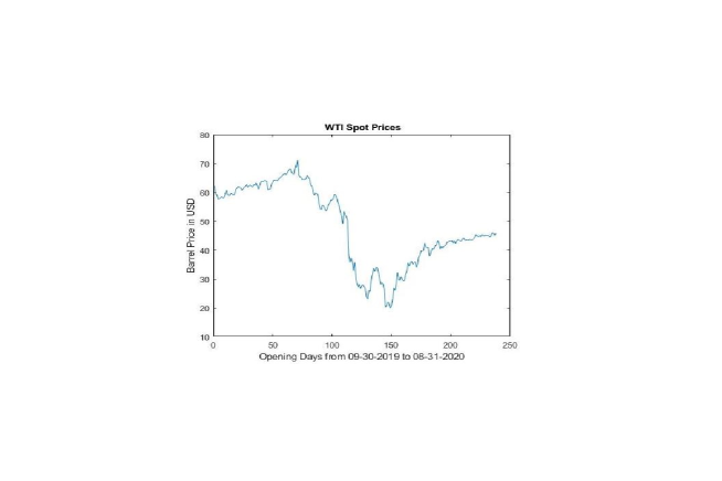
Figure 1: Historical data of Crude Oil Spot Prices - Opening Days from 09/30/2019 to 08/31/2020.

If we look closely the graph, we can observe that the dynamic of the spot price is in three phases during the period of this observation. The first three months are characterized by a slight upward trend, followed by a sharp downturn for another semester and a slight upward trend again.

4.1 Parameters determinants and simulations

We are observing a two state economy: sharp downturn and slight recovery, amid of the global recession around the word. Since the economic regime lasts over a certain period of time, we can use a four stage discrete Markov chain to model the state of the economy. Choose a transition probability matrix $A$ as follows:

$$A=\left(\begin{array}[]{cccc}0.75&0.25&0&0\\ 0.25&0.75&0&0\\ 0&0&0.25&0.7\\ 0&0&0.75&0.25\end{array}\right)$$

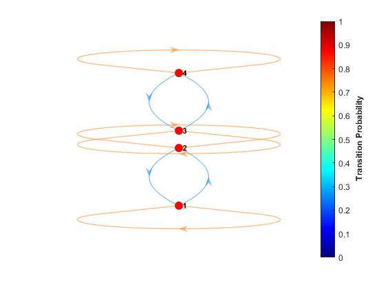
Figure 2: Four Stage Transition Matrix

That is, if the economy is in downturn at time $t$, the probability that it stays in recession is $0.75$. If the economy is growing, the probability that it keeps growing is $0.25$. The zero entries correspond to a stagnation situation, where the economy is staying steady without any significant movement. The Figure 2 is an illustration of these probabilities.

Based on the dynamic of the observed prices, we can calibrate the OU spot prices. Below is a simulated spot price.

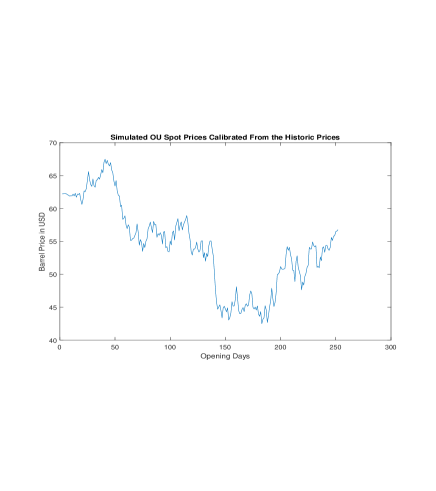
Figure 3: Simulated WTI Crude Oil Spot Prices

Now, we can simulate the dynamic entropic risk associated with each energy derivative product. The parameters of the dynamatic of the spot price are:

Parameters of the Dynamic of the Spot Price
$\alpha$	$\mu$	$\gamma$	Initial Spot Price $S_{0}$
$5$	$\$48.22$	$\$13.66$	$\$62.24$

Table 1: Parameters of the OU Process.

4.2 Sensitivity analysis based on the risk aversion parameter and the time horizon

For different value of $\gamma$, Table 2 presents the value of the entropic risk. Note that the entropic risk does not have an interpretation in term of capital at risk. Figure 4 shows the computed entropic risk for different values of the risk measure parameter $\gamma$. We assume that $\delta_{i}=0.75$, which implies a price decrease of $25\%$. Next, we evaluate the entropic risk associated with the linear derivative for different level of risk aversion.

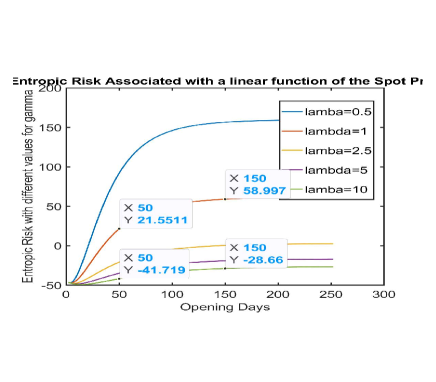
Figure 4: Entropic risk of a linear derivative for different values of gamma

Figure 4 shows the values of the simulated entropic risk. By definition, these vales decrease with respect to $\gamma$. However, these results show that the magnitude of the difference is smaller when $\gamma$ increases. Next, we shall do a quick analysis for some specific values in the Table 2.

	Risk Aversion
Horizon	$\gamma=1$	$\gamma=2.5$	$\gamma=5$	$\gamma=10$
$T=50$ days	21.55	-20.68	-34.74	- 41.72
$T=150$ days	60	0.52	-18.97	- 28.66
Variation ($\%$)	178.42	102.51	45.39	31.30

Table 2: Sensitivity analysis with respect to the risk aversion parameter and the time horizon.

The value of the entropic risk decreases with respect to the risk aversion. This is related to the expression of the entropic risk measure itself. The determinants and estimations of the risk aversion parameter are studied in Bodnar et al. (2018). Usually, the value of the risk aversion depends on the decision maker’s behavior. In Seck et al., (Seck et al. (2012)), it is shown that under the assumption of some particular formulation of a class of risk measures, maximizing a profit subject to these risk constraints is equivalent to maximizing a certain class of multi-attribute utility functions. These multi-attribute utility functions express loss aversion instead of risk aversion. Similar results are obtained recently Bodnar et al. (2018). Thus, the value of the risk aversion parameter depends on the distribution of the underlying asset, which is somehow another way to express the decision maker risk preferences. Another factor that is included in the Table 2 is the time horizon. We can see that, for any values of the risk aversion, the entropic risk associated with the underlying asset decreases as time elapses. To conclude, we are seeing a form of time consistency of the preferences regardless the state of the economy. We observe the same behavior of the entropic risk measure if the underlying assets is a forward contract, see Figure 5 and Table 3.

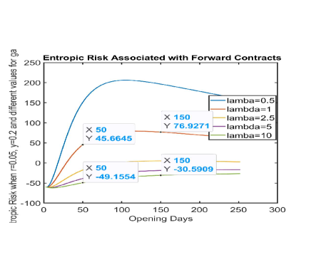
Figure 5: Entropic Risk of Forward Prices for different values of gamma

	Risk Aversion
Horizon	$\gamma=1$	$\gamma=2.5$	$\gamma=5$	$\gamma=10$
$T=50$ days	45.66	-17.60	-38.67	-49.16
$T=150$ days	76.93	5.19	-18.69	-30.59
Variation ($\%$)	68.48	129.49	51.67	37.77

Table 3: Sensitivity analysis with respect to the risk aversion parameter and the time horizon.

4.3 Sensitivity analysis based on the convenience yield

Some historical data analysis has shown that oil futures have reflected a convenience yield of 8% per year on average, from January 1986 to May 2008. The convenience yield is zero or negative if future markets are discouraging storage. This happens recently at the beginning of the Covid-19 health crisis for crude oil commodities; this phenomenon is known as ”backwardization”. Recent study has shown statistical evidence of jump bevahior of the convenience yield in relation to the market conditions such as investment on storage capacity, leasing facility or drilling, see Mason and Wilmot (2020). Next, we analyze the sensitivity of the entropic risk with respect to the convenient yield and the time horizon. Figure 6 provides the rends of the entropic risk for different value of the convenience yield when time elapses. It turns out that for different value of the convenience yield, it will arrive a moment where the entropic risk converge to an equilibrium value. This can be interpreted as a mean-reverting and a term-structure behavior of the convenience yield. That is the behavior of the convenience yield over a short period time might differ over a long period of time. Now, in this context a short period of time could be the order of two to three months. Further studies might determine whether these behaviors of the convenience yield are actually observable in the crude oil market.

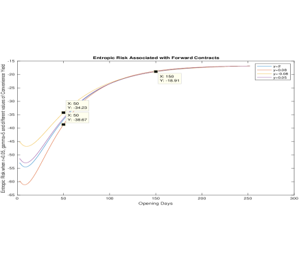
Figure 6: Entropic risk of Future Crude Oil with respect to the convenience yield over time

5 Conclusion

This paper introduces a new class of risk measures that can take into account the decision maker’s preference and the state of the economy. The tractability of these risk measures are studied through simulations on crude oil futures. The results are promising as they show the term structure and the mean-reverting behavior of the convenience yield. However, the determination of the risk aversion parameter in the setting of this paper remains an open topic and requires further studies.

References

- Almansour (2016) Almansour, A. (2016). Convenience yield in commodity price modeling: A regime switching approach. Energy Economics, 53:238–247.
- Alquist et al. (2014) Alquist, R., Bauer, G. H., and Rios, A. D. (2014). What does the convenience yield curve tell us about the crude oil market? Technical report, Bank of Canada.
- Anderson and Mellor (2009) Anderson, L. R. and Mellor, J. M. (2009). Are risk preferences stable? comparing an experimental measure with a validated survey-based measure. Journal of Risk and Uncertainty, 39:137–160.
- Artzner et al. (1997) Artzner, P., Delbaen, F., Eber, J.-M., and Heath, D. (1997). Thinking coherently of risk. Risk, 10(11):68–71.
- Artzner et al. (1999) Artzner, P., Delbaen, F., Eber, J.-M., and Heath, D. (1999). Coherent measures of risk. Mathematical Finance, 9:203–228.
- Baumeister and Kilian (2016) Baumeister, C. and Kilian, L. (2016). Forty years of oil price fluctuations: Why the price of oil may still surprise us. Journal of Economic Perspective s, 30:139–160.
- Ben-Tal and Teboulle (2007) Ben-Tal, A. and Teboulle, M. (2007). An old-new concept of convex risk measures: the optimized certainty equivalent. Mathematical Finance, 17(3):449–476.
- Bodnar et al. (2018) Bodnar, T., Okhrin, Y., Vitlinskyy, V., and Zabolotskyy, T. (2018). Determination and estimation of risk aversion coefficients. Journal of Comput. Manag. Sci., 15:297–317.
- Brandtner et al. (2018) Brandtner, M., Kürsten, W., and Rischau, R. (2018). Entropic risk measures and their comparative statics in portfolio selection: Coherence vs convexity. European Journal of Operational Research, 264:707–716.
- Carmona and Ludkovski (2004) Carmona, R. and Ludkovski, M. (2004). Spot convenience yield models for the energy markets. unpublished.
- Cheridito et al. (2005) Cheridito, P., Delbaen, F., and Kupper, M. (2005). Coherent and convex monetary risk measures for unbounded càdlàg processes. Finance Stochastic, 9(3):369–387.
- Detlefsen and Scandolo (2005) Detlefsen, K. and Scandolo, G. (2005). Conditional and dynamic convex risk measures. Journal of Finance Stochastic, 9(4):539–561.
- Dohmen et al. (2016) Dohmen, T., Lehmann, H., and Norberto, P. (2016). Time varying individual risk attitudes over the great recession: A comparison of germany and ukraine. Journal of Comparative Economics, 44:182–200.
- Dorsman et al. (2013) Dorsman, A., Simpson, J. L., and Westerman, W. (2013). Energy Economics and Financial Markets. Springer, New-York.
- Elliott et al. (1994) Elliott, R. J., Aggoun, L., and Moore, J. B. (1994). Hidden Markov models: estimation and control. Springer, Berlin, Heidelberg, New York.
- Föllmer and Penner (2006) Föllmer, H. and Penner, I. (2006). Convex risk measures and the dynamics of their penalty functions. Journal of Statistics Decisions, 24(1):61–96.
- Gibson and Schwartz (1990) Gibson, R. and Schwartz, E. S. (1990). Stochastic convenience yield and the pricing of oil contingent claims. Journal of Finance, XLV(3):959–976.
- Gollier (2001) Gollier, C. (2001). The economics of risk and time. MIT Press, Cambridge.
- Goovaerts et al. (2004) Goovaerts, M. J., Kaas, R., Laeven, R. J. A., and Tang, Q. (2004). A comonotonic image of independence for additive risk measures. Journal of Insurance: Mathematics and Economics, 35:581–594.
- Hamilton (1989) Hamilton, J. (1989). A new approach to the economic analysis of nonstationary time series and the business cycle. Journal of Econometrica, 57:357–384.
- Kullback and Leibler (1951) Kullback, S. and Leibler, R. A. (1951). On information and sufficiency. The Annals of Mathematical Statistics, 22:79–86.
- Mason and Wilmot (2020) Mason, C. F. and Wilmot, N. A. (2020). Jumps in the convenience yield of crude oil. Journal of Resource and Energy Economics, 60:101163.
- Neely et al. (2014) Neely, C. J., Rapach, D. E., Tu, J., and Zhou, G. (2014). Forecasting the equity risk premium: The role of technical indicators. Journal of Management Science, 60(7):1772–1791.
- Rashid (2008) Rashid, A. (2008). Macroeconomic variables and stock market performance: Testing for dynamic linkages with a known structural break. Journal of Savings and Development, 32(1):77 – 102.
- Ruszczynski and Shapiro (2004) Ruszczynski, A. and Shapiro, A. (2004). Optimization of convex risk functions. Revisited December 22.
- Sánchez and Gallego (2016) Sánchez, F. H. M. and Gallego, V. M. (2016). Parameter estimation in mean reversion processes with deterministic long-term trend. Journal of Probability and Statistics, 2016.
- Schildberg-Horisch (2018) Schildberg-Horisch, H. (2018). Are risk preferences stable? Journal of Economic Perspectives, 32(2):135–154.