Microscopic description of cluster decays based on the generator coordinate method

Abstract

Background: While many phenomenological models for nuclear fission have been developed, a microscopic understanding of fission has remained one of the most challenging problems in nuclear physics.

Purpose: We investigate an applicability of the generator coordinate method (GCM) as a microscopic theory for cluster radioactivities of heavy nuclei, which can be regarded as a fission with large mass asymmetry, that is, a phenomenon in between fission and $\alpha$-decays.

Methods: Based on the Gamow theory, we evaluate the preformation probability of a cluster with GCM while the penetrability of the Coulomb barrier is estimated with a potential model. To this end, we employ Skyrme interactions and solve the one-dimensional Hill-Wheeler equation with the mass octupole field. We also take into account the dynamical effects of the pairing correlation using BCS wavefunctions constructed with an increased strength of the pairing interaction.

Results: We apply this scheme to the cluster decay of ²²²Ra, i.e., ²²²Ra$\to^{14}$C+²⁰⁸Pb, to show that the experimental decay rate can be reproduced within about two order of magnitude. We also briefly discuss the cluster radioactivities of the ²²⁸Th and ²³²U nuclei. For these actinide nuclei, we find that the present calculations reproduce the decay rates with the same order of magnitude and within two or three order of magnitude, respectively.

Conclusions: The method presented in this paper provides a promising way to describe microscopically cluster decays of heavy nuclei.

I INTRODUCTION

Nuclear fission is an important phenomenon in various areas of physics, including productions of neutron-rich nuclei, the r-process nucleosynthesis, and syntheses of superheavy elements [1, 2, 3, 4]. While many phenomenological models for fission have been developed, a microscopic understanding of fission has remained one of the most challenging problems in nuclear physics [5]. In the fission process, many degrees of freedom are involved during a shape evolution of a fissioning nucleus. Since it is difficult to incorporate all the degrees of freedom, it is essential to extract appropriate degrees of freedom for fission. Nuclear deformation parameters are often used for this purpose.

In addition to nuclear deformation, the nuclear superfluidity [6] also plays an important role in describing the fission process, see e.g. Refs. [7, 8, 9, 10]. In particular, the role of dynamical pairing [11] has attracted lots of attention in recent years [12, 13, 14]. To explicitly take into account the pairing dynamics, a pair hopping model was proposed in Ref. [15]. In this model, a nucleus goes into a shape evolution by hopping from one Hartree-Fock configuration to a neighboring configuration by a residual pairing interaction. This model has been successfully applied to recent alpha decay experiments for high spin isomers [16, 17, 18]. Based on a similar idea to the pair hopping model, a more microscopic approach based on a many-body Hamiltonian was investigated in Refs. [19, 20]. Advantages of this approach are i) it is easy to connect to reaction theories [19] and ii) a collective inertia for fission does not need to be evaluated explicitly. Within this model, the effect of the dynamical pairing was considered by introducing the maximum coupling approximation [21], in which the basis states are constructed by increasing the pair correlation.

In this connection, an interesting phenomenon to explore is a cluster radioactivity, such as an emission of ¹⁴C from a heavy nucleus. This phenomenon can be regarded as a phenomenon in between spontaneous fission and $\alpha$ decays. This is a unique phenomenon, in which many-body effects are much more important than $\alpha$ decays, while the matching of a many-body wave function to an external region is much simpler than that for spontaneous fission. The cluster radioactivity was observed for the first time in 1984 in the decay of ²²³Ra emitting the ¹⁴C cluster [22]. Since then, several cluster emission decays have been observed by now [23], in which a daughter nucleus tends to be ²⁰⁸Pb or its neighbors. Notice that the cluster radioactivities may be regarded as a spontaneous fission with large mass asymmetry. See Refs. [24, 25, 26] for recent studies along this line on the cluster radioactivities based on the density functional theory. Even though the branching ratio of the cluster decays to alpha decays is usually considerably small, it has been pointed out that the cluster decay may become a dominant decay mode of superheavy nuclei [25, 26, 27].

In this paper, we apply a similar approach to Refs. [19, 20, 21] to cluster radioactivities of heavy nuclei. While Refs. [19, 20, 21] used a schematic many-body Hamiltonian, we here employ a realistic energy functional of Skyrme type. To this end, we take into account the non-orthogonality of many-body configurations at different shapes by the generator coordinate method (GCM). Also, we consider couplings among all the configurations in a model space, not restricting to the nearest neighbor couplings.

The paper is organized as follows. In Sec. II, we detail the theoretical method for the cluster radioactivities based on the generator coordinate method. In Sec. III, we present results for the cluster decay of ²²²Ra, ²²⁸Th and ²³²U as typical examples. We compare the calculated decay rates with the experimental data as well as with other theoretical calculations. We also discuss the role of dynamical pairing in cluster decays. We then summarize the paper in Sec. IV.

II Cluster decays based on GCM

For a theoretical description of cluster decays, two types of approaches have been employed[23], either based on the Gamow theory for $\alpha$ decays [28] or on models for spontaneous fission. In the former, it is assumed that a cluster is preformed in a mother nucleus and then it tunnels through the Coulomb barrier [29, 30]. In this theory, a decay rate is expressed as

$$w=SfP,$$ (1)

where $S$ is the preformation probability for a cluster to appear in a mother nucleus, $f$ is a barrier assault frequency, i.e., an attempt frequency, and $P$ is the penetration probability of the Coulomb barrier. A similar approach can be formulated also using the Fermi Golden Rule [15]. On the other hand, in the latter approach[24, 25, 26], a potential energy surface and mass inertias for fission characterized by nuclear deformation parameters are calculated based on theoretical models such as the liquid drop model or the density functional theory. The decay rate is estimated from the least action path in the potential energy surface so obtained.

In this paper, we employ the Gamow theory to compute the decay rates. To this end, we estimate the preformation probability $S$ based on the generator coordinate method (GCM), while $f$ and $P$ based on a two-body potential model. That is, we carry out a microscopic calculation before the clusters are preformed using the GCM, while we use a phenomenological two-body approach after that. In principle, we could use the microscopic density functional theory also for the tunneling process. However, this would require a large model space as well as a proper treatment of the neck degree of freedom [24, 31] (see also Ref. [32]). We thus leave it for a future study.

To calculate the preformation probability of a cluster, we first solve the Hartree-Fock (HF) equation with constraints on mass multipole moments. The pairing correlation is also taken into account in the BCS approximation. Following Ref. [24], we use the mass octupole moment, $Q_{3}=\sum_{i}r_{i}^{3}Y_{30}(\theta_{i})$, for the constrained calculations. For the particle-hole interaction, we use the Skyrme interaction with the SkM* [33] and the SLy4 [34] parametrizations. We solve the HF equation using the imaginary-time method with the coordinate-space representation[38]. We impose axial symmetry and use the two-dimensional cylindrical mesh.

For the pairing interaction, we employ a volume-type contact interaction,

$$V_{\rm pair}(\bm{r},\bm{r}^{\prime})=V_{\tau}\,\frac{1-P_{\sigma}}{2}\delta(\bm{r}-\bm{r}^{\prime}),~{}~{}(\tau=n,p)$$ (2)

where $P_{\sigma}$ is the spin exchange operator. The value of $V_{\tau}$ is determined to reproduce the empirical pairing gaps,

$$\begin{split}&\Delta_{n}=-\frac{1}{2}[B(N-1,Z)+B(N+1,Z)-2B(N,Z)],\\ &\Delta_{p}=-\frac{1}{2}[B(N,Z+1)+B(N,Z-1)-2B(N,Z)],\\ \end{split}$$ (3)

where $B(N,Z)$ is the measured binding energy [35] of the nucleus with the neutron number $N$ and the proton number $Z$. For a zero-range pairing interaction, the energy cutoff is necessary to exclude high momentum components from the model space. We use the smooth cut-off procedure with a Fermi function [36, 37].

Based on the idea of GCM[39], we describe the decaying wave function as a superposition of the BCS wave functions at different $Q_{3}$ values,

$$|\Psi\rangle=\sum_{i}f(q_{i})\hat{P}_{Z}\hat{P}_{N}|\Phi(q_{i})\rangle\equiv\sum_{i}f(q_{i})|\Phi(N,Z,q_{i})\rangle,$$ (4)

where $|\Phi(q)\rangle$ is the BCS wave function at $Q_{3}=q$, and $\hat{P}_{Z}$ and $\hat{P}_{N}$ are the operators to project the BCS wave function onto an eigenstate of the proton and the neutron numbers, respectively. The weight function $f(q_{i})$ is determined by solving the Hill-Wheeler equation,

$$\begin{split}&\sum_{j}\langle\Phi(N,Z,q_{i})|H|\Phi(N,Z,q_{j})\rangle f(q_{j})\\ &=E\sum_{j}\langle\Phi(N,Z,q_{i})|\Phi(N,Z,q_{j})\rangle f(q_{j}).\end{split}$$ (5)

The preformation probability $S$ is then determined as

$$S=|g(Q_{t})|^{2},$$ (6)

where $Q_{t}$ corresponds to the octupole moment at the crossing point between the one-body and the two-body configurations (see the discussion below Eq. (16)). Here, the collective wave function $g(q_{i})$ is defined as

$$g(q_{i})=\sum_{j}N^{1/2}(q_{i},q_{j})f(q_{j}),$$ (7)

where $N(q_{i},q_{j})=\langle\Phi(N,Z,q_{i})|\Phi(N,Z,q_{j})\rangle$ is the overlap kernel and $N^{1/2}(q_{i},q_{j})$ is the component of the matrix $N^{1/2}$.

In the usual GCM calculations, the basis function $|\Phi(N,Z,q)\rangle$ is taken to be the local ground state at $q$. Excitations during the decay process can also be taken into using the configuration interaction (CI) approach [19, 20, 21]. That is, instead of Eq. (4), one can consider

$$|\Psi\rangle=\sum_{i}\sum_{k}f_{k}(q_{i})\hat{P}_{Z}\hat{P}_{N}|\Phi_{k}(q_{i})\rangle,$$ (8)

where $\{|\Phi_{k}(q)\rangle\}$ is a set of many-body wave functions at $q$, including both the local ground state and excited states. In Ref. [21], an efficient way to include the excited states has been proposed using the maximum coupling approximation. In this approximation, one modifies the Hamiltonian by increasing the strength of the pairing interaction by a factor $\alpha$,

$$H_{\rm mod}=H_{\rm HF}+\alpha H_{\rm pair},$$ (9)

where $H_{\rm HF}$ and $H_{\rm pair}$ are the particle-hole and the pairing parts of the Hamiltonian, respectively. The local ground state of the modified Hamiltonian, $|\Phi^{(\alpha)}(q)\rangle$, is then superposed as

$$|\Psi\rangle=\sum_{i}f(q_{i})\hat{P}_{Z}\hat{P}_{N}|\Phi^{(\alpha)}(q_{i})\rangle.$$ (10)

The value of $\alpha$ can be determined so that the decay rate is maximized. Notice that using the Thouless theorem[40] the wave function $|\Phi^{(\alpha)}(q_{i})\rangle$ can be expressed as

$$|\Phi^{(\alpha)}(q)\rangle\propto\prod_{i,j}\left(1+C^{(\alpha)}_{i,j}\alpha^{\dagger}_{i}\alpha^{\dagger}_{j}\right)|\Phi(q)\rangle,$$ (11)

where $\alpha_{i}^{\dagger}$ is a creation operator for quasi-particles, thus it includes excited configurations in a specific way.

To compute the frequency $f$ and the penetrability $P$, we consider a phenomenological potential $V$ for the relative motion between the two fragments,

$$V(r)=V_{N}(r)+V_{C}(r),$$ (12)

where $r$ is the relative coordinate, and $V_{N}$ and $V_{C}$ are the nuclear and the Coulomb potentials, respectively. For the Coulomb interaction, $V_{C}$, we consider the potential for a uniformly charged sphere with the radius $r_{C}$,

$$V_{C}(r)=\begin{cases}\frac{Z_{1}Z_{2}e^{2}}{r}&\text{( $r>r_{C}$)}\\ \frac{Z_{1}Z_{2}e^{2}}{r_{C}}(\frac{3}{2}-\frac{r^{2}}{2r^{2}_{C}}),&\text{( $r\leq r_{C}$)}\end{cases}$$ (13)

where $Z_{1}$ and $Z_{2}$ are the proton number of each fragment. We take $r_{C}=1.2(A_{1}^{1/3}+A_{2}^{1/3})$ fm for the charge radius, where $A_{1}$ and $A_{2}$ are the mass number of each fragment. For the nuclear potential, $V_{N}$, we employ a Woods-Saxon potential

$$V_{N}(r)=-\frac{V_{0}}{1+\exp[(r-R_{0})/a]},$$ (14)

for which the radius parameter $R_{0}$ and the diffuseness parameter $a$ are taken from Ref. [41]. The depth parameter $V_{0}$ is adjusted so that the resonance energy of the potential $V$, determined with the two-potential method [42], coincides with the experimental $Q$-value [35]. Even though there may be several uncertainties in the nuclear potential, especially in the region well inside the Coulomb barrier, we would expect that the order of magnitude of a calculated decay rate is rather insensitive once the barrier height is fixed. This is because the decay rate is largely determined by the penetration probability of the Coulomb field; even though the attempt frequency is sensitive to the nuclear potential, it merely changes a multiplicative factor to the decay rate.

With the potential $V$ so determined, we calculate $f$ and $P$ in the WKB approximation as [43],

$$\begin{split}&f^{-1}=\frac{4\mu}{\hbar}\int^{r_{1}}_{r_{0}}\frac{dr}{k(r)}\cos^{2}\left(\int^{r}_{r_{0}}k(r^{\prime})dr^{\prime}-\frac{\pi}{4}\right),\\ &P=\exp\left(-2\int^{r_{2}}_{r_{1}}dr|k(r)|\right),\end{split}$$ (15)

where $r_{i}(i=0,1,2)$ are the classical turning points, with $r_{0}$ and $r_{2}$ being the innermost and the outermost turning points, respectively. $k(r)$ is the local wavenumber defined as $k(r)=\sqrt{2\mu[Q-V(r)]/\hbar^{2}}$, where $\mu$ is the reduced mass for the relative motion between the clusters. Notice that for proton radioactivities the WKB approximation has been shown to agree well with more quantal approaches such as the Green function method and the two-potential method [43]. We expect that the WKB approximation works even better for cluster radioactivities with a larger reduced mass.

To compute the preformation probability $S$ according to Eq. (6), we convert the relative coordinate $r$ to the octupole moment $Q_{3}$ using an approximate formula given by [24]

$$Q_{3}(r)=\sqrt{\frac{7}{4\pi}}\frac{A_{1}A_{2}}{A_{1}+A_{2}}\frac{(A_{1}-A_{2})}{A_{1}+A_{2}}r^{3}.$$ (16)

Notice that the Coulomb potential between the two clusters decreases as a function of $r$, and thus $Q_{3}$, while the one-body energy tends to increase. Both curves will thus cross at a certain octupole moment $Q_{3}$, which we label as $Q_{t}$. In the region of $Q_{3}>Q_{t}$, the total energy becomes smaller when the mother nucleus splits into the two-body system. We therefore regard that the cluster decays happen via this configuration at $Q_{3}=Q_{t}$ and employ Eq. (6) to estimate the cluster preformation probability.

III Results

Let us now apply the model presented in the previous section to the cluster decays of ²²²Ra, ²²⁸Th, and ²³²U and numerically evaluate the decay rates. To this end, we use the cylindrical mesh with $r_{i}=(i-\frac{1}{2})\Delta r,~{}(i=1,2,...14)$ and $z_{j}=(j-\frac{1}{2})\Delta z,~{}(j=-13,-12,..26)$ with $\Delta r=\Delta z=0.8$ fm for the Hartree-Fock+BCS calculations. In addition to the constraint of the mass octupole moment $Q_{3}$, we also impose a constraint on $\langle z\rangle=0$ in order to fix the position of the center of mass.

III.1 ${}^{222}\mathrm{Ra}$

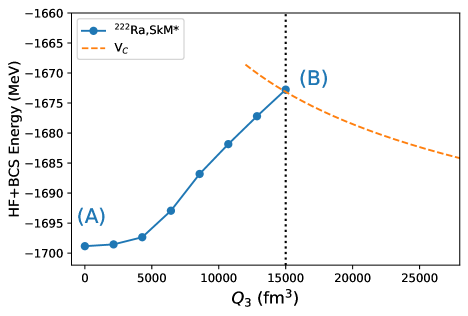
Figure 1: The Hartree-Fock (HF) + BCS energy obtained with the SkM^∗ interaction for the ${}^{222}\mathrm{Ra}$ nucleus as a function of the mass octupole moment, $Q_{3}$. The configuration (A) at $Q_{3}=0$ fm³ corresponds to the ground state in the HF+BCS approximation. The dashed line represents the Coulomb potential for the two-body system ¹⁴C+²⁰⁸Pb. This approaches $E_{\rm gs}-Q$ at large $Q_{3}$, where $E_{\rm gs}$ is the energy for the configuration (A). The configuration (B) at $Q_{3}$=15000 fm³ corresponds to the cluster configuration where the HF + BCS energy crosses the dashed line (see the vertical dotted line).

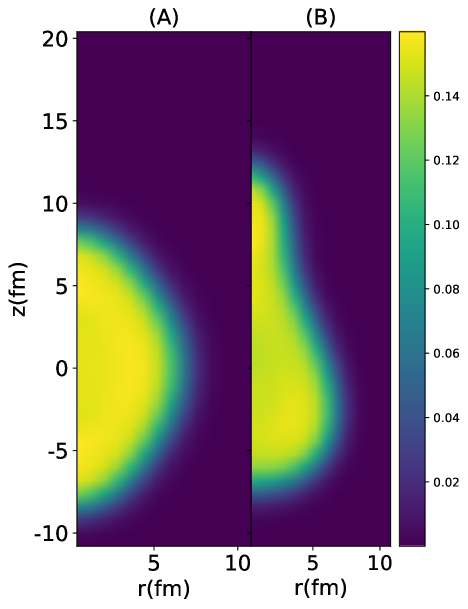
Figure 2: The density distribution of the ${}^{222}\mathrm{Ra}$ nucleus for the configurations (A) and (B) shown in Fig. 1.

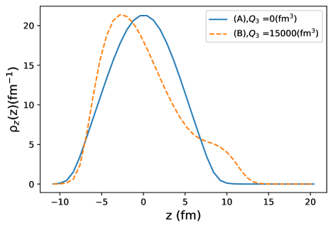
Figure 3: The density distributions corresponding to those shown in Fig. 2 as a function of $z$. Those are obtained by integrating the densities in the $x$ and $y$ directions.

We first discuss the decay of ²²²Ra $\to^{14}$C+²⁰⁸Pb, whose $Q$-value is $Q=33.05$ MeV [35]. We solve the HF + BCS equation with $V_{p}=-398.0$ MeV fm³ and $V_{n}=-280.0$ MeV fm³ for the SkM^∗ interaction, and $V_{p}=-420.0$ MeV fm³ and $V_{n}=-320.0$ MeV fm³ for the SLy4 interaction. The blue solid line in Fig. 1 shows the HF+BCS energy of the ²²²Ra nucleus obtained with the SkM^∗ interaction as a function of the mass octupole moment, $Q_{3}$. The orange dashed line denotes the Coulomb potential, $V_{C}(r(Q_{3}))$, shifted by $E_{\rm gs}-Q$, where $E_{\rm gs}$ is the energy of the ground state in the HF+BCS approximation. In the ground state, denoted by (A) in the figure, ²²²Ra is not octupole deformed. As the octupole deformation is developed, the energy increases and eventually crosses the dashed line at the configuration (B). The density distributions for the configurations (A) and (B) are shown in Fig. 2. See also Fig. 3 for the densities integrated in the $x$ and $y$ directions, $\rho_{z}(z)\equiv\int dxdy\,\rho(\mbox{\boldmath$r$})$. For the configuration (B), the nucleus has a large octupole deformation: the proton and the neutron numbers in the region of $z\geq 8$ fm are 6.41 and 9.50, respectively, close to ¹⁴C. Table 1 summarizes the results of the HF + BCS calculations for the configurations (A) and (B), in which the deformation parameters are defined as

$$\beta_{\lambda}=\frac{4\pi}{3A}\frac{Q_{\lambda}}{\bar{R}^{\lambda}},$$ (17)

with $\bar{R}=\sqrt{\frac{5\langle r^{2}\rangle}{3A}}$, where $\sqrt{\langle r^{2}\rangle}$ is the root-mean-square matter radius and $Q_{\lambda}=\sum_{i}r_{i}^{\lambda}Y_{\lambda 0}(\theta_{i})$ is the mass multpole moments.

Table 1: The results of the Skyrme Hartree-Fock+BCS calculations for the ²²²Ra nucleus. The table summarizes the calculated values for the quadrupole and octupole deformation parameters, $\beta_{2}$ and $\beta_{3}$, the root-mean-square (rms) matter radius, $\sqrt{\langle r^{2}\rangle}$, the rms radius of protons, $\sqrt{\langle r_{p}^{2}\rangle}$, and the total energy, at two different configurations (A) and (B) shown in Fig. 1.

interaction	config.	$\beta_{2}$	$\beta_{3}$	$\sqrt{\langle r^{2}\rangle}$	$\sqrt{\langle r_{p}^{2}\rangle}$	$E$
				(fm)	(fm)	(MeV)
SkM*	(A)	0.229	0.000	5.783	5.695	$-$1697.538
	(B)	0.466	0.553	6.194	6.125	$-$1672.766
SLy4	(A)	0.209	0.000	5.770	5.686	$-$1695.376
	(B)	0.464	0.553	6.196	6.127	$-$1667.459

We next solve the Hill-Wheeler equation (5) in the region of $0\leq Q_{3}\leq Q_{t}=15000$ fm³ with the mesh size of $\Delta Q_{3}=\frac{15000}{7}$ fm³. We have confirmed that the GCM spectrum is almost converged with this mesh size, and moreover, the order of magnitude for the decay rate remains the same even if we employ $\Delta Q_{3}=2000$ fm³ or $\Delta Q_{3}=2400$ fm³. The effect of the number projection is found to be minor, altering the decay rate only by a factor of 2 or smaller. See Table II for the actual values of the decay rates.

Figure 4 shows the square of the collective wave function, $|g(Q_{3})|^{2}$, for the lowest GCM state. As the octupole moment $Q_{3}$ increases, the absolute value of the collective wave function decreases and the value of $S=|g(Q_{t})|^{2}$ at $Q_{3}=Q_{t}$ is in order of $10^{-10}$ for both the interactions.

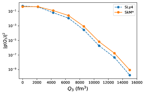
Figure 4: The square of the collective wave function for the GCM ground state of the ²²²Ra nucleus as a function of the octupole moment $Q_{3}$. The solid and the dashed lines show the results with the SkM^∗ and SLy4 interactions, respectively.

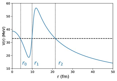
Figure 5: The potential energy between ¹⁴C and ²⁰⁸Pb as a function of the relative distance $r$. The classical turning points are denoted by $r_{0},~{}r_{1}$, and $r_{2}$. The dashed line denotes the $Q$-value ($Q$=33.05 MeV) for the cluster decay of ²²²Ra.

We next evaluate the assault frequency $f$ and the penetrability $P$ based on the potential model as described in Sec. II. The potential between the two fragments is shown in Fig. 5, after the depth parameter of the nuclear interaction is adjusted to reproduce the resonance energy. The resultant depth parameter is $V_{0}=67.64$ MeV, whereas the radius and the diffuseness parameters are $R_{0}=9.99$ fm and $a=0.63$ fm, respectively. The dashed line corresponds to the $Q$ value of the cluster decay. With this parameter set, the assault frequency and the penetrability are found to be $f=8.29\times 10^{20}$ s^-1 and $P=4.10\times 10^{-26}$, respectively.

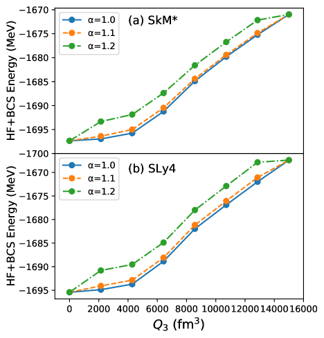
Figure 6: Similar to Fig. 1, but obtained with the BCS wave function for the modified Hamiltonian, Eq. (9). Notice that the energy shown is defined as the expectation value of the original Hamiltonian with $\alpha=1$. The upper and the lower panels show the results of the SkM^∗ and the SLy4 interactions, respectively.

In order to investigate the effect of dynamical pairing, we next apply the maximum coupling approximation[21]. Figure 6 shows the HF+BCS energy for three different values of $\alpha$ in Eq. (9). Notice that we fix the value of $\alpha$ to be 1 for the configurations at $Q_{3}=0$ and $Q_{3}=Q_{t}$, while for the other configurations we solve the HF+BCS equations with the modified Hamiltonian. The expectation value of the original Hamiltonian is then computed with the wave functions so obtained. Since such wave functions contain excited states components (see Eq. (11)), the total energy increases for $\alpha\neq 1$. On the other hand, the off-diagonal components of the overlap kernel tends to be increased when $\alpha$ is varied from one. These two effects compete with each other in evaluating the decay rates.

Figure 7(a) shows the preformation probability $S=|g(Q_{t})|^{2}$ as a function of $\alpha$. The corresponding decay rate $w$ is shown in Fig. 7(b). Because of the competition of the two opposite effects mentioned in the previous paragraph, a peak structure appears in the decay rate, at $\alpha=1.075$ and $\alpha=1.1$ for the SkM^∗ and the SLy4 interactions, respectively, similar to the previous studies on the role of dynamical pairing in spontaneous fission [12, 14, 21]. The decay rate at the peak is larger than the decay rate for the original pairing strength (i.e., $\alpha=1$) by a factor of 1.82 and 2.04 for the SkM^∗ and SLy4, respectively. Notice that the decay rate with SkM^∗ is larger than that with SLy4. This is because the energy difference between the configurations (B) and (A) is larger with SLy4 (see Table I).

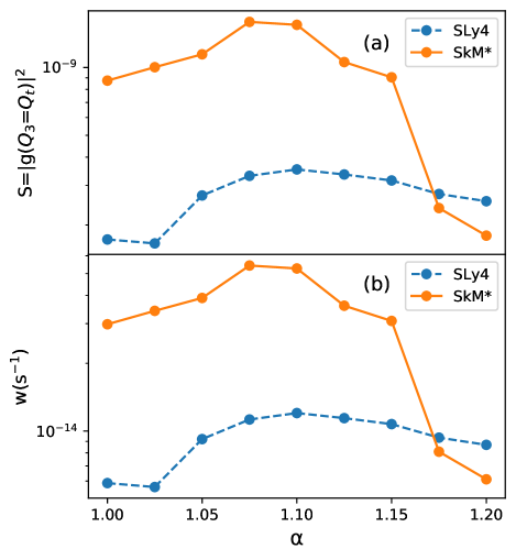
Figure 7: The preformation probability (the upper panel) and the decay rate (the lower panel) for the cluster decay ²²²Ra$\rightarrow^{208}$Pb+¹⁴C for various values of $\alpha$ for the maximum coupling approximation.

The decay rates at the maxima in Fig. 7(b) are summarized in Table II together with the experimental data. For comparison, the calculated result without the number projection is also listed. The present calculations reproduce the experimental deta within two orders of magnitude, that would be reasonable as a microscopic calculation for fission. In the Table, we also compare our results to the calculated result of Ref. [24] with the Gogny D1S interaction, which uses the model based on the WKB approximation for spontaneous fission with the least action path. One can see that the degree of agreement of our results with the data is comparable to that of the result of Ref. [24].

Table 2: The decay rates $w$ for the cluster decay of ²²²Ra $\rightarrow^{208}$Pb+¹⁴C obtained with the present approach. They are compared to the experimental data and to the theoretical calculation [24] based on the WKB model with the least action fission path.

$w~{}(\mathrm{s}^{-1})$	the method
$5.43\times 10^{-14}$	GCM (SkM*)
$8.15\times 10^{-14}$	GCM without the projection (SkM*)
$1.20\times 10^{-14}$	GCM (SLy4)
$8.73\times 10^{-10}$	the least action (Gogny D1S) [24]
$6.7~{}(\pm 1.8)\times 10^{-12}$	Price et al.[44]
$5.6~{}(\pm 2.2)\times 10^{-12}$	Hourani et al. [45]
$4.20~{}(\pm 1.18)\times 10^{-12}$	Hussonnois et al. [46]

III.2 ${}^{228}\mathrm{Th}$ and ${}^{232}\mathrm{U}$

We next discuss the cluseter decay of ²²⁸Th $\rightarrow^{208}$Pb+²⁰O and ²³²U $\rightarrow^{208}$Pb+²⁴Ne. The $Q$-values of these decays are 44.72 MeV and 62.33 MeV. The octupole moment at $Q_{t}$ reads $Q_{t}=2.0\times 10^{4}$ fm³ and $2.4\times 10^{4}$ fm³ for ²²⁸Th and ²³²U, respectively. The calculated decay rates are shown in Fig. 8 as a function of $\alpha$ for the maximum coupling approximation. To this end, we use the mesh size of $\Delta Q=2000$ fm³ to discretize the Hill-Wheeler equation. For these nuclei, the collective wave functions at $Q_{3}=Q_{t}$ are as small as the order of 10^-6, and thus it easily suffers from numerical instabilities. In order to avoid this, we extrapolate the wave function in the region of 6000 $\leq Q_{3}\leq 12000$ fm³ down to $Q_{t}$. The qualitative features of the decay rates are the same as those for ²²²Ra discussed in the previous subsection. That is, the decay rate is enhanced by several times by introducing the effect of dynamical pairing, and the calculated decay rates reproduce the experimental data within the same order for ²²⁸Th and within two or three orders of magnitude for ²³²U. See Table III for a summary of the calculated results.

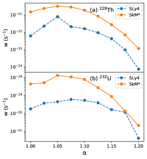
Figure 8: Same as Fig. 7(b), but for ²²⁸Th $\rightarrow^{208}$Pb+²⁰O (the upper panel) and ²³²U $\rightarrow^{208}$Pb+²⁴Ne (the lower panel).

Table 3: Same as Table II, but for ${}^{228}\mathrm{Th}\rightarrow^{208}\mathrm{Pb}+^{20}\mathrm{O}$ and ${}^{232}\mathrm{U}\rightarrow^{208}\mathrm{Pb}+^{24}\mathrm{Ne}$.

the nucleus	$w~{}(\mathrm{s}^{-1})$	the method
228Th	$3.20\times 10^{-21}$	GCM (SkM*)
	$7.96\times 10^{-22}$	GCM (SLy4)
	$2.05\times 10^{-20}$	the least action [24]
		(Gogny D1S)
	$1.29~{}(\pm 0.22)\times 10^{-21}$	Bonetti et al. [47]
232U	$1.32\times 10^{-18}$	GCM (SkM*)
	$6.03\times 10^{-20}$	GCM (SLy4)
	$3.10\times 10^{-24}$	the least action [24]
		(Gogny D1S)
	$6.3~{}(\pm 1.5)\times 10^{-22}$	Barwick et al. [48]
	$2.72~{}(\pm 0.23)\times 10^{-21}$	Bonetti et al. [49]
	$2.83~{}(\pm 0.22)\times 10^{-21}$	Bonetti et al.[50]

IV Summary

Using the generator coordinate method, we have estimated microscopically the preformation probabilities for the cluster radioactivities of ²²²Ra, ²²⁸Th and ²³²U. Unlike the pair hopping model, we have taken into account the non-orthogonality of the configurations as well as non-nearest neighbor couplings. Moreover, we have employed the maximum coupling approximation to take into account the effect of dynamical pairing. By combining with the Gamow theory, we have shown that the experimental decay rate for ²²²Ra is reproduced reasonably well with this calculation and the same is true for ²²⁸Th and ²³²U even though there is some uncertainty derived from the fitting. We have also shown that the dynamical pairing increases the preformation probability by a factor of two or three.

In this paper, we have used the octupole moment as a generator coordinate. In principle, one can also incorporate explicitly other degrees of freedom, such as the quadrupole moment, the hexadecapole moment, and the neck degree of freedom. In particular, the neck has been known to play an important role in treating the scission dynamics and thus a connection between a one-body system to a two-body system. By taking into account the neck degree of freedom, the preformation probability of a cluster may also be better defined. This will be an interesting future problem, even though a numerical accuracy of a GCM solution would be more demanding.

The cluster decay can be regarded as a phenomenon in between spontaneous fission and $\alpha$ decays. The method presented in this paper opens a novel and promising way to develop a unified microscopic description for quantum tunneling decays of nuclear many-body systems, including $\alpha$ decays, cluster decays, and spontaneous fission. For spontaneous fission, the Gamow theory cannot be applied in a straightforward manner, since the barrier penetration and a formation of fission fragments are strongly coupled to each other. Extending the method presented in this work to such a problem would also be an interesting future work.

- [1] R. Vandenbosch and J.R. Huizenga, Nuclear Fission (Academic Press, New York, 1973).
- [2] H.J. Krappe and K. Pomorski, Theory of Nuclear Fission (Springer-Verlag, Heidelberg, 2012).
- [3] P. Fröbrich and R. Lipperheide, Theory of Nuclear Reactions (Oxford University Press, Oxford, 1996).
- [4] N. Schunck and L. M. Robledo, Rep. Prog. Phys. 79 116301 (2016).
- [5] M.Bender et al., J. Phys. G: Nucl. Part. Phys. 47 113002 (2020).
- [6] D.M. Brink and R.A. Broglia, Nuclear Superfluidity: Pairing in Finite System (Cambridge University Press, 2005).
- [7] G. Schütte and L. Wilets, Nucl. Phys. A 252, 21 (1975).
- [8] G. Schütte and L. Wilets, Z. Phys. A 286, 313 (1978).
- [9] G. Scamps, C. Simenel, and D. Lacroix, Phys. Rev. C 92, 011602(R), 2015.
- [10] K. Washiyama, N. Hinohara, and T. Nakatsukasa, Phys. Rev. C 103, 014306 (2021).
- [11] L.G. Moretto and R.P. Babinet, Phys. Lett. B 49, 147 (1974).
- [12] S. A. Giuliani, L. M. Robledo, and R. Rodríguez-Guzmán, Phys. Rev. C 90, 054311 (2014).
- [13] J.Sadhukhan, J. Dobaczewski, W. Nazarewicz, J. A. Sheikh, and A. Baran, Phys. Rev. C 90, 061304(R) (2014).
- [14] R. Rodríguez-Guzmán and L. M. Robledo, Phys. Rev. C 98, 034308 (2018).
- [15] F. Barranco, G. Bertsch, R. Broglia, and E. Vigezzi, Nucl. Phys. A 512, 253 (1990).
- [16] J. Rissanen, R.M. Clark, A.O. Macchiavelli, P. Fallon, C.M. Campbell, and A. Wiens, Phys. Rev. C 90, 044324 (2014).
- [17] R.M. Clark and D. Rudolph, Phys. Rev. C 97, 024333 (2018).
- [18] R.M. Clark et al., Phys. Rev. C 99, 024325 (2019).
- [19] G. F. Bertsch, Phys. Rev. C 101, 034617 (2020).
- [20] K. Hagino and G. F. Bertsch, Phys. Rev. C 101, 064317 (2020).
- [21] K. Hagino and G. F. Bertsch, Phys. Rev. C 102, 024316 (2020).
- [22] H. J. Rose and G. A. Jones, Nature 307, 245 (1984).
- [23] D. S. Delion, Theory of Particle and Cluster Emission (Springer-Verlag, Heidelberg, 2010).
- [24] M. Warda and L.M. Robledo, Phys. Rev. C 84, 044608 (2011).
- [25] M. Warda, A. Zdeb, and L.M. Robledo, Phys. Rev. C 98, 041602(R) (2018).
- [26] Z. Matheson, S.A. Giuliani, W. Nazarewicz, J. Sadhukhan, and N. Schunck, Phys. Rev. C 99, 041304(R) (2019).
- [27] D.N. Poenaru, R.A. Gherghescu, and W. Greiner, Phys. Rev. C 85, 034615 (2012).
- [28] G. Gamow, Zeitschrift für Physik 51, 204 (1928).
- [29] R. Blendowske, T. Fliessbach, and H. Walliser, Nucl. Phys. A 464, 75 (1987).
- [30] D. Delion, A. Insolia, and R. Liotta, J. Phys. G: Nucl. Part. Phys. 20, 1483 (1994).
- [31] R. Han, M. Warda, A. Zdeb, and L.M. Robled, Phys. Rev. C 104, 064602 (2021).
- [32] N.-W. T. Lau, R.N. Benard, and C. Simenel, arXiv:2111.06513.
- [33] J. Bartel, P. Quentin, M. Brack, C. Guet, and H. B. Håkansson, Nucl. Phys. A. 386, 79 (1982).
- [34] E. Chabanat, P. Bonche, P. Haensel, J. Meyer, and R. Schaeffer, Nucl. Phys. A. 635, 231 (1998).
- [35] M. Wang, W. Huang, F. Kondev, G. Audi, and S. Naimi, Chin. Phys. C 45, 030003 (2021).
- [36] P. Bonche, H. Flocard, P.H. Heenen, S.J. Krieger, and M.S. Weiss, Nucl. Phys. A 443, 39 (1985).
- [37] S.J. Krieger, P. Bonche, H. Flocard, P. Quentin, and M.S. Weiss, Nucl. Phys. A 517, 275, (1990).
- [38] K. T. R. Davies, H.Flocard, S.Krieger, and M.S.Weiss, Nucl. Phys. A 342, 111 (1980).
- [39] P. Ring and P. Schuck, The Nuclear Many-Body Problem (Springer-Verlag, Berlin, 2000).
- [40] D. J. Thouless, Nucl. Phys. 21, 225 (1960).
- [41] R. A. Broglia and A. Winther, Heavy ion reactions, vol. I (Benjamin, Reading 1981).
- [42] S. A. Gurvitz, P. B. Semmes, W. Nazarewicz, and T. Vertse, Phys. Rev. A 69, 042705 (2004).
- [43] S. Åberg, P. B. Semmes, and W. Nazarewicz, Phys. Rev. C 56, 1762 (1997).
- [44] P. B. Price, J. D. Stevenson, S. W. Barwick, and H. L. Ravn, Phys. Rev. Lett. 54, 297 (1985).
- [45] E. Hourani, M. Hussonnois, L. Stab, L. Brillard, S. Gales, and J. P. Schapira, Phys. Lett. B 160, 375 (1985).
- [46] M. Hussonnois, J. F. Le Du, L. Brillard, J. Dalmasso, and G. Ardisson, Phys. Rev. C 43, 2599 (1991).
- [47] R. Bonetti, C. Chiesa, A. Guglielmetti, C. Migliorino, A. Cesana, and M. Terrani, Nucl. Phys. A 556, 115 (1993).
- [48] S. W. Barwick, P. B. Price, and J. D. Stevenson, Phys. Rev. C 31, 1984 (1985).
- [49] R. Bonetti, E. Fioretto, C. Migliorino, A. Pasinetti, F. Barranco, E. Vigezzi, and R. A. Broglia, Phys. Lett. B 241, 179 (1990).
- [50] R. Bonetti, C. Chiesa, A. Guglielmetti, C. Migliorino, A. Cesana, M. Terrani, and P. B. Price, Phys. Rev. C 44, 888 (1991).