Simulating macroscopic quantum correlations in linear networks

Abstract

Many developing quantum technologies make use of quantum networks of different types. Even linear quantum networks are nontrivial, as the output photon distributions can be exponentially complex. Despite this, they can still be computationally simulated. The methods used are transformations into equivalent phase-space representations, which can then be treated probabilistically. This provides an exceptionally useful tool for the prediction and validation of experimental results, including decoherence. As well as experiments in Gaussian boson sampling, which are intended to demonstrate quantum computational advantage, these methods are applicable to other types of entangled linear quantum networks as well. This paper provides a tutorial and review of work in this area, to explain quantum phase-space techniques using the positive-P and Wigner distributions.

I Introduction

There is a widespread interest in current physics in the immense variety of macroscopic quantum correlations that can occur in physical systems that are not in thermal equilibrium. Examples include quantum networks, which are a growing area of modern quantum technology. These may operate either in a transient mode [1], or in the steady-state [2]. In contrast to traditional condensed matter physics, these are typically very far from being homogeneous. Such networks are qualitatively different to small systems with low excitation and are also distinct from thermal equilibrium studies in many-body systems [3], since external inputs drive them into non-thermal-equilibrium states.

Systems of this type are both highly challenging and fascinating to modern physicists from several points of view. The challenging aspect is that they are hard to solve. Macroscopic quantum networks have an exponentially large Hilbert space [4]. This generally rules out exact orthogonal basis methods, for example by expanding in the usual basis of number states. Analytic solutions for the density matrix are rare. Even these are not always as useful as one might expect, due to difficulties in computationally evaluating the solutions except as averages over many possible implementations [5].

The fascination of these systems is that they are an unknown territory. Sending probes to Mars is challenging, but even on Mars, telescopes give us an idea of what to expect. Macroscopic quantum networks, because of their exponential complexity and lack of analytic solutions, have few scientific precedents. As well as giving rise to macroscopic Bell violations, such networks introduce the issue of computational complexity, which is simply that some calculations may take enormously long times. Quantum correlations occur that may not cause a Bell violation, but are still classically ruled out in a more subtle way. Some correlations are computationally prohibited classically.

In addition to their fundamental interest, there is an increasingly important potential in quantum technology. Some commonly researched applications are to novel types of sensors [6, 7] or metrological devices [8, 9, 10]. Additionally, there are new types of quantum computers, whose purpose is to perform a task that is thought to be impossible using classical means [11]. These include Gaussian boson samplers [12] and the coherent Ising machine (CIM) [13], which have now been scaled to larger sizes than conventional gate-based quantum computers [14, 2]. The reason for this is that they have a much simpler design than conventional quantum logic gate approaches. In the simplest cases they have only linear coupling [15] or just one type of nonlinearity and no logic gates [16]. In a similar way, reduced instruction set classical computers [17] are often more scalable than older designs with large instruction sets.

There is an ongoing debate about the advantages and limitations of such devices, as well as the potential for verifying their behavior, given the essential Hilbert space complexity. This leads to a distinction between types of classical simulation, which we explain. While direct simulations of every counting event are possible for small networks [18, 19, 20, 21], these rapidly become impossible at larger sizes, and may take billions of years [1]. Despite this, one may still be able to use phase-space methods to simulate photon-counting probabilities, which allows verification of important network characteristics [22, 23, 24]. Such results are not restricted to low-order correlations, and can test for decoherence and high order correlations.

Because this is a large and rapidly growing field, only a few aspects of this work can be covered here. We treat linear networks, and nonlinear cases such as the CIM are given elsewhere [25]. It is hoped that by giving the basics of this work, the reader may be motivated to investigate further. The main point emphasized is that even with growing network complexity, there are theoretical tools available to analyze them. One cannot make predictions to $12$ decimals. However, one can still compare models with experimental measurements, which is essential both to test the theory and to improve the experiments.

II Phase-space simulations

Why are quantum networks theoretically challenging?

The main feature of a quantum network is the number of modes involved. This leads to exponential growth in the Hilbert space dimension. As an illustration, if one has $100$ qubits, which have a basis of spin up and down, there are $d=2^{100}\approx 10^{30}$ quantum states. The systems treated here comprise $M$ modes labelled $j=1,..,M$, and with boson annihilation operators $\hat{a}_{j}$. Recent experiments have already employed $M>100$ modes [14] in a linear network. Bosonic modes, with more than two states, have an even faster growth in dimension.

To store the quantum amplitudes of even $10^{30}$ states with 15 decimal precision requires $\sim 10^{32}$ bits. As of 2021, the world’s fastest classical supercomputer [26], Fugaku, has an enormous $10^{16}$ bit memory. However, this is a factor of $10^{16}$ too small even to store the quantum state, let alone compute high order correlations. Such limitations prevent the direct use of exact number state methods for calculations in large quantum networks.

In one-dimensional lattices with low excitations and nearest-neighbor couplings, one may approximate a large network by many smaller ones. This gives rise to approximations known as the density matrix renormalization group, or tensor network methods [27]. Such methods can fail when there is increased connectivity. An example of this is if there is increased dimensionality, or extended correlations across the entire network, which may lead to all of the modes being correlated.

Fortunately, there are other techniques available. One can carry out probabilistic simulations in a phase-space which allows a complete representation of the density matrix. Wigner [28] first showed how to map quantum wave-functions onto a distribution function on a phase-space of classically meaningful quantities, although this is only probabilistic in some cases. The general concept of a phase-space representation in quantum mechanics is a correspondence between a set of phase-space variables and a set of quantum operators with a particular ordering [29]. Subsequent work was motivated by the idea [30] that one can use such methods to calculate the dynamics of the observables. It is these that are measurable and of most scientific interest.

The first probabilistic quantum phase-space distribution was developed by Husimi [31], using the concept of a coherent state [32, 33]. Later this was shown to lead to an anti-normally ordered bosonic field representation [34], called the Q-function, which provides a positive representation of quantum fields. Normally ordered representations on a classical phase-space, called P-representations, are useful for simulating lasers, but are singular for non-classical states. There is a range of classical phase-space methods of this type, often called $s$-ordered [34]. Glauber’s P-representation was later extended to a non-classical phase-space with double the classical dimensions, called the positive P-representation. This is normally ordered and always exists as a smooth, positive distribution for any quantum state [35, 36].

The positive P-representation gives results with comparable sampling errors to photon-counting experiments. In both cases, one measurement or one random sample must be repeated many times to give overall averages. There are statistical errors, but experimental measurements have the same issue. Other phase-space representations can be singular or negative, or have larger sampling errors for photon counting. Wigner phase-space representations are best for a special case: Gaussian initial states combined with linear or weakly nonlinear networks and homodyne detectors, rather than photon-counting [37].

There are also proposals for similar techniques using modified Wigner functions in qubit-based systems [38, 39] which are largely outside the scope of this tutorial, and are not treated here.

II.1 Wigner representation

The oldest method for quantum phase-space is the Wigner representation of bosonic states [28, 40]. This provides a method for random simulations, provided the Wigner distribution is positive and has a corresponding stochastic process. Such techniques can treat linear networks or nonlinear quantum networks at large occupation numbers [37, 41], in excellent agreement with experiment.

This distribution can be written as:

$$W\left(\boldsymbol{\alpha}\right)=\frac{1}{\pi^{2N}}\int d^{2}\mathbf{z}\left\langle e^{i\mathbf{z}\cdot\left(\hat{\mathbf{a}}-\boldsymbol{\alpha}\right)+i\mathbf{z}^{*}\cdot\left(\hat{\mathbf{a}}^{\dagger}-\boldsymbol{\alpha}^{*}\right)}\right\rangle.$$ (1)

Operator mean values are obtained using a mapping with symmetric ordering, of form:

$$\left\langle\hat{a}_{i}^{\dagger m}\dots\hat{a}_{j}^{n}\right\rangle_{SYM} =\int d^{2}\boldsymbol{\alpha}\left[\alpha_{i}^{*m}\ldots\alpha_{j}^{n}\right]W\left(\boldsymbol{\alpha}\right).$$ (2)

This is a particularly useful approach for networks that employ homodyne detectors. These measure quadratures $\hat{x}_{i}^{\theta_{i}}=\hat{a}e^{-i\theta_{i}}+\hat{a}^{\dagger}e^{i\theta_{i}}$, which are commonly used to characterize squeezing or entanglement.

For a positive Wigner function, the symmetrically ordered moments of quadrature readouts are equivalent to random samples of the Wigner distribution [34], with

$$\left\langle\hat{x}_{i}^{\theta_{i}}\dots\hat{x}_{j}^{\theta_{j}}\right\rangle_{SYM} =\left\langle x_{i}^{\theta_{i}}\ldots x_{j}^{\theta_{j}}\right\rangle_{W}.$$ (3)

Here, the $x$ and $p$ quadratures are defined as

$$\hat{x}_{i}=\hat{x}_{i}^{0} =\hat{a}+\hat{a}^{\dagger},$$

$$\hat{p}_{i}=\hat{x}_{i}^{\pi/2} =i\left(\hat{a}^{\dagger}-\hat{a}\right).$$ (4)

Provided the initial state is Gaussian and either the Hamiltonian is linear or the photon numbers are large, the Wigner distribution is positive and can be readily sampled stochastically. The calculation of the moments is efficient, scaling linearly with the system-size, provided the samples are available. A Wigner simulation under these conditions is directly equivalent to an experimental readout of measured quadratures [37, 42], where $x_{i}^{\theta_{i}}=\alpha e^{-i\theta_{i}}+\alpha^{*}e^{i\theta_{i}}$ corresponds to the measured quadrature current. The reason for this is that third-order terms in the propagation equations vanish either in the limit of linear couplings or large photon number, so an initially positive distribution, such as a Gaussian distribution, will remain positive. To make use of this property one needs to generate random samples, which is treated below for the case of linear network experiments.

These conditions are very restrictive, however. Linear network experiments can also use particle detectors, which are equivalent to normal ordering. Such detectors can’t be efficiently treated using the Wigner representation, unless corrections are included which transform the ordering from symmetric to normal. However, the additional vacuum noise inherent in the Wigner representation means that there is a rapidly growing sampling error for high order correlations, reducing the scalability. Similarly, if there are nonlinearities, a Wigner simulation will omit certain nonlinear quantum noise corrections.

The other phase-space representations such as the Husimi Q-function, for anti-normal ordering, and Glauber’s P-representation, for normal ordering, have their own drawbacks. Similar to the Wigner function, the Q-function suffers from large sampling errors while the P-representation has highly singular distributions for the non-classical inputs present in linear network experiments.

II.2 Generalized P-representation

The generalized P-representation [35, 43] was developed as the quantum successor to Glauber’s P-representation, as it always has a positive distribution for any quantum state. This is the most efficient representation for simulating normally-ordered photon detectors, due to its ability to use efficient stochastic sampling methods to generate input probabilities.

This method expands the density matrix over a multi-dimensional subspace of the complex plane, defined as:

$$\hat{\rho}=\Re\iint P\left(\boldsymbol{\alpha},\boldsymbol{\beta}\right)\hat{\Lambda}\left(\boldsymbol{\alpha},\boldsymbol{\beta}\right)\mathrm{d}\mu\left(\boldsymbol{\alpha},\boldsymbol{\beta}\right),$$ (5)

where, by only taking the real part, the output is always hermitian. The basis operator

$$\hat{\Lambda}\left(\boldsymbol{\alpha},\boldsymbol{\beta}\right)=\frac{|\boldsymbol{\alpha}\rangle\langle\boldsymbol{\beta}^{*}|}{\langle\boldsymbol{\beta}^{*}|\boldsymbol{\alpha}\rangle},$$ (6)

projects the density matrix onto multi-mode coherent states [44], while $\mathrm{d}\mu\left(\boldsymbol{\alpha},\boldsymbol{\beta}\right)$ is an integral measure on the $2M$-dimensional complex space of coherent state amplitudes $\boldsymbol{\alpha},\boldsymbol{\beta}$. The definition of the integral measure determines whether the distribution $P\left(\boldsymbol{\alpha},\boldsymbol{\beta}\right)$ is positive or complex valued. We use the positive distribution here where $\mathrm{d}\mu\left(\boldsymbol{\alpha},\boldsymbol{\beta}\right)\equiv d^{2}\boldsymbol{\alpha}d^{2}\boldsymbol{\beta}$ corresponds to a $4M$-dimensional real Euclidean volume.

Number state inputs can also be simulated, but for greater sampling efficiency, the complex P-representation is preferable for such inputs. To simulate these cases, an additional complex factor $\Omega$ should be used, when sampling the distribution [22, 23].

Besides computational efficiency, the generalized P-representation has the added benefit of making normally ordered operator moments equal to stochastic moments [35, 45, 46]:

$$\left\langle\hat{a}_{j_{1}}^{\dagger},\dots,\hat{a}_{j_{n}}\right\rangle=\left\langle\beta_{j_{1}},\dots,\alpha_{j_{n}}\right\rangle_{P},$$ (7)

where quantum expectation values are denoted $\left\langle\right\rangle$, and averages obtained using the generalized P-representation are $\left\langle\right\rangle_{P}$. This allows one to simply replace quantum operators with stochastic variables without changing the analytical solutions. As in the Wigner case, high-order moments are efficiently calculable in times that scale linearly with system-size, provided samples are available.

The following sections demonstrate how to efficiently generate the samples, which have now reached $16,000$ modes. The main memory limitation is the storage of the experimental $M\times M$ transmission matrix data, explained below.

II.3 Simulating Gaussian inputs

Any algorithm that simulates correlations of a complex system such as a linear bosonic network must be tested against exactly known distributions. Provided they have positive distributions, the Wigner and generalized P-representation are both well suited to simulating Gaussian distributions such as thermal and squeezed distributions. The phase-space distributions are themselves Gaussian in these cases.

To simulate any phase-space representation, one must first generate stochastic samples. For Gaussian quantum inputs into a network, the corresponding phase-space representations are also Gaussian. As a result, they are completely defined by their means - which we take as zero here - and their second-order correlations.

We define an ordering parameter $\sigma$ to signify the amount of vacuum noise in an operator ordering. Compared to the $s$-ordering in earlier conventions [40], $\sigma=\left(1-s\right)/2$. Thus, $\sigma=0$ signifies normal ordering, $\sigma=\frac{1}{2}$ symmetric ordering, and $\sigma=1$ anti-normal ordering. For independent quantum inputs, with no correlations between the real and imaginary quadratures, we define the general $\sigma$-ordered quadrature variance as

$$\left\langle\left\{\left(\Delta\hat{x}_{j}\right)^{2}\right\}_{\sigma}\right\rangle =\left(\Delta_{\sigma j}^{x}\right)^{2}=2\left(n_{j}+\sigma+\tilde{m}_{j}\right)$$

$$\left\langle\left\{\left(\Delta\hat{y}_{j}\right)^{2}\right\}_{\sigma}\right\rangle =\left(\Delta_{\sigma j}^{y}\right)^{2}=2\left(n_{j}+\sigma-\tilde{m}_{j}\right).$$ (8)

Here, $n_{j}=\left\langle\hat{a}_{j}^{\dagger}\hat{a}_{j}\right\rangle$ and $\tilde{m}_{j}=\left\langle\hat{a}_{j}\hat{a}_{j}\right\rangle$ which are defined in terms of linear bosonic networks in Section III A. Since the phase-space quadratures are:

$$x_{i}^{\theta_{i}}=\alpha e^{-i\theta_{i}}+\beta e^{i\theta_{i}},$$ (9)

we can now generate stochastic samples in any representation by simply matching the $\sigma$ parameter to the type of representation and generating random Gaussian samples from

$$\alpha_{j} =\left(\Delta_{\sigma}^{x}w_{j}+i\Delta_{\sigma}^{y}w_{j+M}\right)/2$$

$$\beta_{j} =\left(\Delta_{\sigma}^{x}w_{j}-i\Delta_{\sigma}^{y}w_{j+M}\right)/2.$$ (10)

The terms $w_{j}$ are uncorrelated Gaussian real random numbers with unit variance, thus requiring $2M$ random Gaussian numbers per phase-space sample. This is the most computationally efficient method for generating samples of each representation. Here $\beta\equiv\alpha^{*}$ in the case of the Wigner representation, which uses a classical phase-space, with $\sigma=1/2$. The positive P-representation has $\sigma=0$, and can have $\beta\neq\alpha^{*}$ if either of $\Delta_{\sigma}^{x}\,$ or $\,\Delta_{\sigma}^{y}$ from Eq.(8) are imaginary. Here $\Delta_{\sigma}^{x}\,$ or $\,\Delta_{\sigma}^{y}$ can be imaginary if $n_{j}<\left|\tilde{m}_{j}\right|$, in the positive P-representation.

These variances are related to the squeezed-state parameters in the next section. Phase-space simulations do not always replicate observable random outputs. This depends on the type of mapping used. In this tutorial we will first treat normally ordered mappings for photon counting detectors, which replaces an experimental discrete integer variable by a complex variable with identical correlations. We will also consider Wigner representations, where the stochastic process is indistinguishable from an experimental output.

When conducting simulations in phase-space one must obtain averages over a large number of samples, and for any ensemble average to be reliable, the calculation must be repeated multiple times for each input mode. Generally, the more the simulation is repeated, the more accurate the ensemble averaged output will be, with smaller errors.

The sampling error $e_{s}$ scales with the number of samples as $1/\sqrt{S}$ [23]. For any accurate simulation of an experimental system, the theoretical sampling error must be smaller than the experimental sampling error. One can either continuously increase the number of samples computed in parallel, or else one can simply increase the number of times the calculation is repeated, although this does increase computation time significantly, if multi-core computations aren’t possible.

III Linear bosonic networks

Linear bosonic networks may appear trivial, since the quantum correlations have exact analytic solutions. However, when mode numbers are large, these analytic solutions can become exponentially hard to compute, resulting in matrix permanents [15], Hafnians [47] or Torontonians [48]. Consequently, most output correlations cannot be exactly computed in large systems with $M\apprge 60$ modes.

In recent experiments with $M=100$ modes [1], a direct simulation was estimated, in 2019, to take nearly a billion years, with the world’s fastest supercomputer. Improved algorithms have now been proposed to reduce the classical simulation time [49]. These are also exponentially slow, meaning that they become impractical with even small size increases.

The cause of the problem is that the analytic expressions for correlations may involve combinatoric expressions with exponentially many terms. Therefore, having an analytic solution does not eliminate the problem of Hilbert space dimension. These solutions can still take exponentially long to calculate. Just as seriously, they produce round-off errors which grow rapidly [50]. This is the basis for the boson sampling quantum computer. These devices generate random numbers that cannot be generated efficiently by classical means [15, 4], by measuring photon detection events, or counts, in each mode.

Since one cannot compute the output correlations for large networks exactly, an intriguing issue arises. How does one verify that the computer is working? This is similar to testing problems related to environmental standards [51]. One has to ask: was the test carried out correctly? With quantum computers there is a new question: can a test be carried out at all? Many proposed tests are restricted to low order correlations [52, 53, 54] which cannot uniquely characterize the output distributions, because these in general require all orders to characterize [55]. Other proposed tests require different experimental configurations, meaning that the actual GBS data is not used [56].

This can be answered, at least in part, through the use of sampled correlations and probabilities, as explained in the next section.

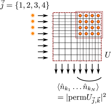
Figure 1: Schematic of a boson sampling experiment. This shows a simple, $8\times 8$ unitary transformation with four single photon inputs. A measurement of the correlated outputs is given by the permanent function which is exponentially hard to compute exactly for large matrices. The much larger, more recent GBS experiments use squeezed inputs, have decoherence, and employ highly efficient on-off detectors.

III.1 Input quantum states

The original iteration of the boson sampling quantum computer sent single photon Fock states into an optical network, the output of which is then measured using photon detectors [12]. An inability to scale the size of the network to computationally interesting regimes due to constraints in generating single, indistinguishable photons [57, 58, 59] has driven a push to seek alternative, experimentally accessible bosonic networks.

One such network replaces the number state with a Gaussian single-mode squeezed state as the nonclassical light source [47]. This type of linear bosonic network is called a Gaussian boson sampler (GBS). It has recently been implemented in multiple large scale experiments with $100$ modes or more, claiming to calculate samples with a Torontonian distribution [1]. A GBS sends $N\subset M$ single-mode squeezed states into an optical network which is described by the linear, unitary transformation matrix $\boldsymbol{T}$. The input modes are transformed by the matrix into $M$ output modes, allowing measurements to be made on the output state $\hat{\rho}^{(out)}$.

The input state $\hat{\rho}^{(in)}$ can be defined as a product of single-mode pure squeezed states

$$\hat{\rho}^{(in)}=\prod_{j}\left|\boldsymbol{r}_{j}\right\rangle\left\langle\boldsymbol{r}_{j}\right|,$$ (11)

with squeezing vector $\boldsymbol{r}=\left[r_{1},\dots,r_{N}\right]$, if each input mode $N$ is independent. Using the squeezed state expansion $\left|r\right\rangle=\hat{S}\left(r\right)\left|0\right\rangle$, where $\hat{S}\left(r\right)$ is the squeezing operator, the input photon number can be found from the expectation of the single-mode number operator

$$n\left(r_{j}\right) =\left\langle\hat{a}_{j}^{\dagger}\hat{a}_{j}\right\rangle$$

$$=\sinh^{2}\left(r_{j}\right).$$ (12)

The corresponding coherence of the input photons can similarly be defined as

$$m\left(r_{j}\right) =\left\langle\hat{a}_{j}^{2}\right\rangle$$

$$=\sinh\left(r_{j}\right)\cosh\left(r_{j}\right).$$ (13)

The normally ordered variances of the quadrature operators $\hat{x}_{j}=\hat{a}_{j}+\hat{a}_{j}^{\dagger}$ and $\hat{y}_{j}=\left(\hat{a}_{j}-\hat{a}_{j}^{\dagger}\right)/i$, with commutation relation $\left[\hat{x}_{l},\hat{y}_{j}\right]=2i\delta_{lj}$, are well documented for pure squeezed states and can be written in terms of the input photon number and coherence for the generalized P-distribution, as

$$\left\langle\left(\Delta\hat{x}_{j}\right)^{2}\right\rangle =2\left(n+m\right)=e^{2r_{j}}$$

$$\left\langle\left(\Delta\hat{y}_{j}\right)^{2}\right\rangle =2\left(n-m\right)=e^{-2r_{j}}.$$ (14)

This is easily expressed in any ordering as

$${\left\langle\left\{\left(\Delta\hat{x}_{j}\right)^{2}\right\}_{s}\right\rangle} {=2\left(n+\sigma+m\right)}$$

$${\left\langle\left\{\left(\Delta\hat{y}_{j}\right)^{2}\right\}_{s}\right\rangle} {=2\left(n+\sigma-m\right).}$$ (15)

Experiments that generate squeezed states usually have additional decoherence caused by longitudinal mode mismatching [1] or other dephasing effects [23]. To accurately simulate bosonic networks one must include decoherence. An approximate model for decoherence consists of an intensity transmissivity $T=1-\epsilon$, which reduces the input photon intensity while adding $n_{j}^{th}=\epsilon n_{j}$ thermal photons per mode. Although the output photon number is unchanged, the coherence of each mode is now given by

$$\left\langle\hat{a}_{j}^{2}\right\rangle=\tilde{m}=\left(1-\epsilon\right)m\left(r_{j}\right).$$ (16)

The addition of decoherence alters the input modes, which can no longer be considered simply pure squeezed states, and have variances given by Eq (8), which now include decoherence in each mode. Although the relationship is similar to Eq (14), the variances can no longer be simplified to $\exp\left(\pm 2r_{j}\right)$, which increases their product above the Heisenberg limit. These more realistic states are also called thermal squeezed states in the literature, usually with other parameterizations [60].

III.2 Sampling squeezed phase-space distributions

The normal ordering of the photo-detectors used to measure the output state, and its non-singular nature for squeezed states makes the generalized P-representation the most efficient phase-space representation to simulate GBS. However, before we can sample the output state, we must first generate the input state in the generalized P-representation.

This is straightforwardly applied by initially neglecting the added input mode decoherence, this is added later with the beam splitter model of decoherence described above when the stochastic samples are generated. Since our input is a pure squeezed state, and recalling that a squeezed state corresponds to a superposition of coherent states, we can expand the density matrix, Eq.(11), using the coherent state expansion [61]

$$\left|r\right\rangle=C\int_{-\infty}^{\infty}\mathrm{d}\alpha_{x}\exp\left(-\alpha_{x}^{2}/\gamma\right)\left|\alpha_{x}\right\rangle.$$ (17)

Here, $\left|\alpha_{x}\right\rangle$ is a Glauber coherent state [33], $\alpha_{x}$ in this case is a real number and $C=(1+\gamma)^{1/4}/\sqrt{\pi\gamma}$ is the normalization constant with $\gamma=e^{2r}-1$.

Once expanded, the input density matrix is given by:

$$\hat{\rho}^{(in)}=\Re\iint P\left(\boldsymbol{\alpha}_{x},\boldsymbol{\beta}_{x}\right)\hat{\Lambda}\left(\boldsymbol{\alpha}_{x},\boldsymbol{\beta}_{x}\right)\mathrm{d}\boldsymbol{\alpha}_{x}\mathrm{d}\boldsymbol{\beta}_{x},$$ (18)

with corresponding quadrature variables,

$$\boldsymbol{x} =\boldsymbol{\alpha}+\boldsymbol{\beta}$$

$$\boldsymbol{p} =\frac{\left(\boldsymbol{\alpha}-\boldsymbol{\beta}\right)}{i}.$$ (19)

and an input distribution:

$$P\left(\boldsymbol{\alpha},\boldsymbol{\beta}\right)=\prod_{j}C_{j}e^{-\left(\alpha_{xj}^{2}+\beta_{xj}^{2}\right)\left(\gamma_{j}^{-1}+1/2\right)+\alpha_{xj}\beta_{xj}}\delta\left(\alpha_{yj}\right)\delta\left(\beta_{yj}\right),$$ (20)

where $C_{j}=\sqrt{1+\gamma_{j}}/\left(\pi\gamma_{j}\right)$ is the normalization constant. The distribution $P\left(\boldsymbol{\alpha},\boldsymbol{\beta}\right)$ is a positive, Gaussian distribution which is restricted to the real axes and is obtained using the inner product of two coherent states

$$\left\langle\beta_{x}\mid\alpha_{x}\right\rangle=e^{\alpha_{x}\beta_{x}-\frac{1}{2}\left(\alpha_{x}^{2}+\beta_{x}^{2}\right)},$$ (21)

which is also needed to construct the projection operator. For any input defined as a product of single-mode squeezed states, Eq.(20) always exists.

In order to simulate any phase-space representation, one must first generate stochastic samples of the initial quantum state. However, each phase-space representation samples the initial state differently, leading to different sampling errors for the same initial state depending on the representation. Unlike the Wigner and Q-function representations, the generalized P-representation has a much smaller sampling error due to it not containing additional vacuum noise [23]. This is another reason why the generalized P-representation is the most efficient representation to simulate GBS.

Generating stochastic samples for the pure-state input distribution, Eq. (20), is straightforward for Gaussian states. Using the real Gaussian noises $\left\langle w_{i}w_{j}\right\rangle_{P}=\delta_{ij}$, we wish to construct the random samples $\overrightarrow{\alpha}=\left[\boldsymbol{\alpha},\boldsymbol{\beta}\right]=\left[\alpha_{1},\dots,\alpha_{2M}\right]$ which is achieved using the stochastic model given above for a pure squeezed state [23]

$$\alpha_{j}^{0} =\delta_{j+}w_{j}+\delta_{j-}w_{j+M}$$

$$\beta_{j}^{0} =\delta_{j+}w_{j+M}+\delta_{j-}w_{j}.$$ (22)

Here, $\delta_{j\pm}$ is a real Gaussian sample with solution $\delta_{j\pm}^{2}=\frac{1}{2}\left(m_{j}\pm\sqrt{n_{j}}\right)$. However, since our input state isn’t a simple pure squeezed state, we must alter the stochastic model to include the intensity transmissivity and additional thermal photons per mode. The full stochastic random samples are therefore expressed as in the general form of Eq (10). The additional decoherence has the added effect of changing our input distribution, which is no longer always restricted to the real axes in thermalized cases.

III.3 Effect of the linear network

Once the input stochastic samples have been generated, they are transformed using the linear transformation matrix $\boldsymbol{T}$. We define this as an $M\times M$ complex matrix, which is measured in the experimental network. The transformed amplitudes, $\boldsymbol{\alpha}^{\prime}=\boldsymbol{T}\boldsymbol{\alpha}$ and $\boldsymbol{\beta}^{\prime}=\boldsymbol{T}^{*}\boldsymbol{\beta}$, are then used to sample the output state

$$\hat{\rho}^{(out)}=\Re\iint P\left(\boldsymbol{\alpha},\boldsymbol{\beta}\right)\hat{\Lambda}\left(\boldsymbol{T}\boldsymbol{\alpha},\boldsymbol{T}^{*}\boldsymbol{\beta}\right)\mathrm{d}\mu\left(\boldsymbol{\alpha},\boldsymbol{\beta}\right),$$ (23)

from which photon counting measurements are taken. For a lossless network, $\boldsymbol{T}$ is a unitary matrix, but generally it is non-unitary due to losses. Since coherent states remain coherent even with absorption, the above transformation is still valid for the positive P-representation, even when $\boldsymbol{T}$ is not unitary. For the Wigner representation, one can transform the amplitudes so that $\boldsymbol{\alpha}^{\prime}=\boldsymbol{T}\boldsymbol{\alpha}$ only in the unitary case; otherwise additional noise terms are needed [24].

IV Measurements in Gaussian boson sampling

The photo-detectors, or click detectors, used in boson sampling experiments saturate for more than one count at a detector. To clarify, a “click” is a detection event, while a “count” is the number of measured photons. Each detector therefore outputs binary numbers $c_{j}=0,1$ which, for $M$ modes, produces point patterns represented as a vector $\boldsymbol{c}$. There are $2^{M}$ possible patterns available, where total probability of any individual click pattern is therefore $2^{-M}$, which is exponentially small for large $M$, provided that they are equally probable.

Each detector is defined by the projection operator

$$\hat{\pi}_{j}\left(c_{j}\right)=:e^{-\hat{n}^{\prime}_{j}}\left(e^{-\hat{n}^{\prime}_{j}}-1\right)^{c_{j}}\colon,$$ (24)

the expectation of which, $\left\langle\hat{\pi}_{j}\left(c_{j}\right)\right\rangle$, is the probability of observing a single count at the $j$-the detector, where $\hat{n}^{\prime}_{j}$ is the output photon number. For a bosonic network with $M$ detectors [62], the multi-click projection operator becomes:

$$\hat{\Pi}\left(\boldsymbol{c}\right)=\bigotimes_{j=1}^{M}\hat{\pi}_{j}\left(c_{j}\right),$$ (25)

which is the product of projection operators at each detector. For Gaussian inputs, the expectation, $\left\langle\hat{\Pi}\left(\boldsymbol{c}\right)\right\rangle$, is the probability of observing any single binary pattern. This is the Torontonian function [48]. For example, if $M=6$, the binary pattern $\left[1,1,1,0,0,0\right]$ has the projector:

$$\hat{\Pi}\left(\boldsymbol{c}\right)=\hat{\pi}_{1}\left(1\right)\hat{\pi}_{2}\left(1\right)\hat{\pi}_{3}\left(1\right)\hat{\pi}_{4}\left(0\right)\hat{\pi}_{5}\left(0\right)\hat{\pi}_{6}\left(0\right).$$ (26)

which is a product of three click projectors in the first three detectors followed by three non-click projections. This binary pattern has a probability of $2^{-6}\approx 0.016$ which, although small, is still easily computed classically.

Upon inspection, it is clear how Eq. (25) becomes exponentially complex as $M$ increases, from recent experiments [1] an $M=100$ network has a probability of $2^{-100}\approx 10^{-31}$ of observing a single binary pattern. One is more likely to win the lottery multiple times than to observe a single binary pattern. We have now arrived at the crux of the verification problem with linear bosonic networks. How can the outputs be verified when the probability of obtaining any individual click pattern is nearly zero? We note that it is known that there are computational reasons why one cannot directly classically generate such counts in a reasonable time. However, the sparseness of the probabilities is still be an issue even if one could classically generate them.

To answer this, we use binning. Binning is the common approach of combining large, sparse sums of data into discrete bins in order to obtain reproducible statistics. Applying it to the output of a bosonic network, one can combine exponentially many click patterns into bins based on the number of photon counts. This allows one to calculate grouped count probabilities, which is the probability of observing $m$ counts in any pattern, as opposed to explicitly simulating discrete experimental photon counts.

Consider the probability of observing $\boldsymbol{m}=\left(m_{1},\dots,m_{g}\right)$ grouped counts in $S_{1},S_{2},\dots$ disjoint sets of $\boldsymbol{M}=\left(M_{1},M_{2},\dots\right)$ output modes, while disregarding the counts in any other modes. This is a marginal probability if $n=\sum_{j=1}^{g}M_{j}<M$, and it requires summing over all patterns which satisfy the condition that the counts for the detectors in the set $S_{1}$ sum up to $m_{1}$, the counts in $S_{2}$ sum up to $m_{2}$, or in general, that:

$$m_{j}=\sum_{i\in S_{j}}c_{i}.$$ (27)

This result is achieved on defining a general grouped count correlation as

$$\mathcal{G}_{M}^{(n)}\left(\boldsymbol{m}\right)=\left\langle\prod_{j=1}^{g}\left[\sum_{\sum c_{i}=m_{j}}\hat{\Pi}_{S_{j}}\left(\boldsymbol{c}\right)\right]\right\rangle.$$ (28)

Here, $n=\sum_{j=1}^{g}M_{j}\leq M$ is the total correlation order following the standard definition of Glauber [44]. For example, if there is only one mode, it is a first order correlation, if there are two modes it is a second-order correlation. The full probability of a given pattern, the Torontonian, is obtained by taking $n=M$ and $\boldsymbol{M}=\left(1,1,\dots\right)$.

Applications to various experimental correlations are easily illustrated. This approach is essential for experiments. By grouping patterns together, one can transform a sparse distribution to a non-sparse one, for which probabilities can be estimated from the data. For example, the probability of observing a single count at the $j$-th detector, is obtained when $n=1$ and $M_{j}=1$, giving $\mathcal{G}_{1}^{(1)}\left(\boldsymbol{m}\right)=\left\langle\hat{\pi}_{j}\left(c_{j}\right)\right\rangle$. This corresponds to the expectation of Eq. (24). Similarly, one can sum over all $n-th$ order correlations.

At first glance, it might appear that grouped correlations only introduce added difficulty to the problem of verification. If one cannot compute the Torontonian, how is it possible to sum over exponentially many different Torontonians? This seems just like asking a runner who has never finished a marathon, to run one every day for a year. However, with phase-space methods the computational problem is sampling error, rather than the order itself. By adding many terms, the relative sampling error is reduced. This makes this hard calculation feasible.

To show how this works, note that since $\hat{\pi}_{j}$ is normally ordered, it can be readily simulated by simply replacing it with the phase-space observable

$$\pi_{j}\left(c_{j}\right)=e^{-n^{\prime}_{j}}\left(e^{-n^{\prime}_{j}}-1\right)^{c_{j}},$$

where $n^{\prime}_{j}$ is sampled from the output state, Eq.(23), with probability $P\left(\boldsymbol{\alpha},\boldsymbol{\beta}\right)$. However the question still remains about how to efficiently calculate an exponentially large summation. Fortunately, this is achievable, through the use of Fourier transforms, as shown in earlier work on number-counting methods for boson sampling [22]. By introducing the angles $\theta_{i}=2\pi/\left(M_{i}+1\right)$ together with the Fourier observable

$$\tilde{\mathcal{G}}_{M}^{(n)}\left(\boldsymbol{k}\right)=\left\langle\prod_{j=1}^{g}\bigotimes_{i\in S_{j}}\left(\pi_{i}\left(0\right)+\pi_{i}\left(1\right)e^{-ik_{i}\theta_{i}}\right)\right\rangle_{P},$$ (29)

with $k_{i}=0,\dots m_{i}$, one can use a multi-dimensional, inverse discrete Fourier transform to calculate the grouped correlations as

$$\mathcal{G}_{M}^{(n)}\left(\boldsymbol{m}\right)=\frac{1}{\prod\left(M_{i}+1\right)}\sum_{\boldsymbol{k}}\tilde{\mathcal{G}}_{M}^{(n)}\left(\boldsymbol{k}\right)e^{i\sum k_{i}\theta_{i}m_{i}}.$$ (30)

The inverse Fourier transform reduces the computational complexity of the sums by removing all patterns which don’t contain $\boldsymbol{m}$ counts. Therefore, grouped correlations can be used obtain measurable, statistical fingerprints of an experimental network that are also computable.

IV.1 Phase-space algorithm

So far we have described the theoretical tools necessary to verify the output correlations of a GBS network using grouped correlations sampled from the generalized P-representation. An efficient algorithm has been developed which implements these tools and was recently applied to a $100$-mode GBS experiment by Zhong et al [1], showing excellent agreement between theory and experiment when decoherence was included [24]. In this section we will outline the details of this algorithm and present results of various tests that were conducted to verify the simulated correlations.

Simulating ensemble averaged grouped correlations using the discrete Fourier transform technique introduced in Eq. (30) is straight forward and computationally efficient for most observables. One must simply loop over the count projector $\pi_{j}$, taking the product over input samples before calculating the ensemble average for each $k_{i}$. The discrete Fourier transform is then applied to all ensemble averages giving the grouped correlations of a particular observable.

Multi-dimensional binning of the grouped correlations is more challenging, although also giving far more points of comparison. This is highly desirable, to provide a means to distinguish experimental data from direct classical simulations with ’fake’ algorithms. A grouped correlation can be binned into $D$-dimensions, giving the probability of observing $n=m_{1},\dots,m_{M/D}$ counts in each dimension. To simulate this, the input samples must be partitioned into bins corresponding to the number of dimensions. The count projector is then calculated for each $k_{i}$ as before, however this occurs over each partitioned separately before a multi-dimensional discrete Fourier transform is applied to the ensemble average of each partition.

For smaller dimensions, this does not take a significant amount of time to compute. However, as the dimensionality increases, up to $M$ dimensions being theoretically possible, the computation time increases significantly. Memory constraints from the increased ensemble size start to occur. Another practical issue is that increased dimensionality leads to fewer experimental or computational samples per bin. If either of these are too small, the comparisons lose significance. This requires an understanding of statistical tests.

When verifying correlations of large complex experimental networks, one must make sure sufficient statistical tests are conducted to verify the simulated correlations. Although this is the case with any comparison of theory with experiment, it is even more important when decoherence is included, as small alterations in the input mode decoherence can greatly affect the output grouped correlations. To quantify this, a chi-square test is used to compare phase-space simulations with GBS experimental correlations. Chi-square tests are commonly used to calculate the differences between theoretical and experimental measurements for independent samples, and are widely used to validate random number generators. We use a standard definition of the chi-square test

$$\chi_{c}^{2}=\sum_{i=1}^{k}\frac{\left(\bar{P}_{i}-P_{i}^{e}\right)^{2}}{\sigma_{i}^{2}},$$ (31)

which assumes theoretical and experimental correlations are independent and approximately Gaussian. The theoretical probability $\bar{P}_{i}$ is obtained by averaging over phase-space ensembles where, for large ensemble numbers, $\bar{P}_{i}$ converges to the true theoretical probability $P_{i}$. The experimental probability $P_{i}^{e}$ is obtained from experimental data or numerically calculated in the case of exactly known distribution tests. The variance is given by $\sigma_{i}^{2}=\sigma_{e,i}^{2}+\bar{\sigma}_{s,i}^{2}$ and is defined as the sum of the experimental and simulated variances respectively. For distributions which are approximately Gaussian, chi-square tests are expected to produce results of $\chi_{c}^{2}/k\approx 1$ for $k$ valid bins. We define a valid bin as a bin with more than $10$ counts.

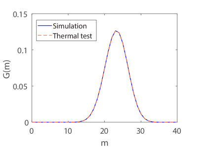
Figure 2: Comparison of theory with an exactly known uniform thermal distribution of total counts $\mathcal{G}_{40}^{(40)}\left(\boldsymbol{m}\right)$ with $1.2\times 10^{6}$ ensembles for a $M=40$ GBS network. The solid blue line is the theoretical prediction, while the orange dash line is exact distribution.

Before this algorithm was applied to experimental GBS data, it was thoroughly tested against a variety of exactly known distributions with a large variety of modes. One such test, is the simulation of total counts, $\mathcal{G}_{M}^{(M)}\left(\boldsymbol{m}\right)$, which is the probability of observing $n=M$ counts in any pattern. Comparisons with an exactly known uniform thermal distribution for an $M=40$ mode GBS, are shown in Fig. (2). We see excellent agreement between simulated and thermal correlations which is validated by a chi-square test result of $\chi_{therm}^{2}/k=1.0\pm 0.3$ for $k=32$ valid bins. Comparisons of total counts for a non-uniform squeezed distribution with $M=100$ modes are also given in Fig. (3), which again shows excellent agreement with simulated correlations.

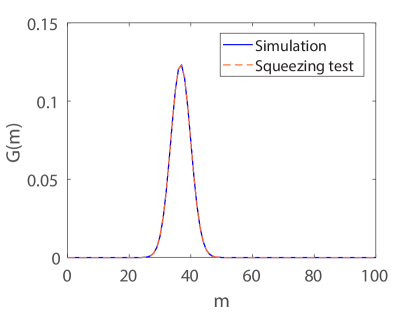
Figure 3: Comparison of theory with an exactly known non-uniform squeezed distribution with $M=100$ mode GBS network. Solid blue line is theoretical prediction of total counts, $\mathcal{G}_{100}^{(100)}\left(\boldsymbol{m}\right)$, while the orange dash line is the squeezed distribution.

Another test is shown in Fig. (4), which is a two-dimensional binning, , $\mathcal{G}_{M/2,M/2}^{(M)}\left(\boldsymbol{m}\right)$, of the grouped correlations for the $M=100$ mode non-uniform squeezed distribution. Chi-square tests were negligible on this scale, being well within the acceptable margin for an exact distribution.

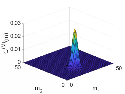
Figure 4: Simulation of a non-uniform squeezed distribution for $M=100$ modes with a two-dimensional binning, $\mathcal{G}_{50,50}^{(100)}\left(\boldsymbol{m}\right)$.

The graphs given here are just a small fraction of the possible distributions one can obtain using grouped correlations. The excellent agreement of these tests shows how grouped correlations, simulated using stochastic sampling techniques obtained from the generalized P-representation, provide a possible answer to the question of verification of linear bosonic networks. However, a verification algorithm is only useful if it can simulate correlations in less than exponential time, and this is where the real benefit of grouped correlations becomes apparent. The exact phase-space simulations shown here took $<50s$ on a desktop computer, while $100$-mode GBS simulations took $\sim 100s$ [24].

This is orders of magnitude faster than direct simulation methods, which makes these techniques useful for verification. While up to $16,000-$th order has been already investigated, these are much more challenging, due to time and memory constraints.

V N-partite entanglement

Linear networks generate nonclassical, entangled states. But how does one verify and classify such complex, high-order entanglement?

We now consider the generation and detection of an $M$-partite entangled state using a Gaussian network, expanding on work presented earlier [24]. The quadrature phase amplitudes are defined as $\hat{x}_{j}=\hat{a}_{j}+\hat{a}_{j}^{\dagger}$ and $\hat{p}_{j}=\frac{1}{i}(\hat{a}_{j}-\hat{a}_{j}^{\dagger})$, in an appropriate rotating frame. Here, we give an account of how an $M$-partite entangled state can be generated with just one or two squeezed input beams, and also discuss the concept of steering for these multipartite entangled states.

These signatures can all be very easily simulated in phase-space, due to the direct correspondence of quadrature measurements to Wigner phase-space simulations for such Gaussian states. We note that this correspondence is no longer valid for nonlinear networks with small photon numbers.

V.1 Two-mode EPR entanglement

Two-mode Einstein-Podolsky-Rosen (EPR) entanglement is created by combining one or two squeezed modes across a beam splitter, which we label $BS1$. This concept was explained for a single squeezed input in Reid [63]. More details are given in [24, 64]. The experimental configuration that allows the creation of two-mode EPR entanglement is given in Fig. 5.

Figure 5: Generation of two-mode Einstein-Podolsky-Rosen (EPR) entanglement. Two squeezed modes $\hat{a}_{1}^{in}$, $\hat{a}_{2}^{in}$ are combined using a beam splitter labelled $BS1$, that has a reflectivity $R_{1}^{2}$. The two entangled output modes are $\hat{a}_{1}^{\left(1\right)}$ and $\hat{a}_{2}^{\left(1\right)}$. The first input mode is squeezed in the $p$-quadrature, i.e. $\Delta^{2}\hat{p}_{1}^{in}=e^{-2r_{1}}$, while the second input mode is squeezed in the $x$-quadrature with $\Delta^{2}\hat{x}_{2}^{in}=e^{-2r_{2}}$. As mentioned in the main text, a choice of $R_{1}=1/\sqrt{2}$, together with these squeezed inputs, lead to the expressions $\Delta^{2}\left(\hat{x}_{1}^{\left(1\right)}-\hat{x_{2}}^{\left(1\right)}\right)=2e^{-2r_{2}}$ and $\Delta^{2}\left(\hat{p}_{1}^{\left(1\right)}+\hat{p}_{2}^{\left(1\right)}\right)=2e^{-2r_{1}}$, in (37).

We consider the unitary transformation represented as

$$\hat{a}_{1}^{(1)} = R_{1}\hat{a}_{1}^{in}+T_{1}\hat{a}_{2}^{in}$$

$$\hat{a}_{2}^{(1)} = T_{1}\hat{a}_{1}^{in}-R_{1}\hat{a}_{2}^{in}$$ (32)

where $R_{1}^{2}$ is the beam splitter reflectivity and $T_{1}^{2}=1-R_{1}^{2}$ is the transmission coefficient, and we take $R_{1}$ and $T_{1}$ as real and positive. A phase shift may be necessary as well as the beam splitter to achieve this transformation. The inputs are given as $\hat{a}_{j}^{in}$. The two outputs of the beam splitter are given as $\hat{a}_{j}^{(1)}$. For convenience, we denote the variance of an observable $\hat{x}$ by $\Delta^{2}\hat{x}\equiv(\Delta\hat{x})^{2}=\langle\hat{x}^{2}\rangle-\langle\hat{x}\rangle^{2}$. Let us suppose $a_{2}^{in}$ is a squeezed vacuum with

$$\Delta^{2}\hat{x}{}_{2}^{in}=e^{-2r_{2}},$$ (33)

and $a_{1}^{in}$ is squeezed vacuum with

$$\Delta^{2}\hat{p}{}_{1}^{in}=e^{-2r_{1}}.$$ (34)

Here $r_{j}>0$ is the squeezing parameter. We assume minimum uncertainty states where $(\Delta\hat{x}{}_{j}^{in})(\Delta\hat{p}{}_{j}^{in})=1$. For $r_{j}=0$, there is no squeezing.

Using (32), the variances of the two outgoing fields can be evaluated. We find on rearranging,

$$\hat{a}_{1}^{in} = R_{1}\hat{a}_{1}^{(1)}+T_{1}\hat{a}_{2}^{(1)}$$

$$\hat{a}_{2}^{in} = T_{1}\hat{a}_{1}^{(1)}-R_{1}\hat{a}_{2}^{(1)}.$$ (35)

Hence,

$$R_{1}\hat{p}_{1}^{(1)}+T_{1}\hat{p}_{2}^{(1)} = \hat{p}_{1}^{in}$$

$$T\hat{x}_{1}^{(1)}-R_{1}\hat{x}{}_{2}^{(1)} = \hat{x}_{2}^{in},$$ (36)

which, for a 50/50 beam splitter where $R_{1}=T_{1}=\frac{1}{\sqrt{2}}$, leads to $\hat{x}_{1}^{(1)}-\hat{x}{}_{2}^{(1)}=\sqrt{2}\hat{x}_{2}^{in}$ and $\hat{p}_{1}^{(1)}+\hat{p}_{2}^{(1)}=\sqrt{2}\hat{p}_{1}^{in}$. Therefore,

$$\Delta^{2}(\hat{x}_{1}^{(1)}-\hat{x}_{2}^{(1)}) = 2e^{-2r_{2}}$$

$$\Delta^{2}(\hat{p}_{1}^{(1)}+\hat{p}_{2}^{(1)}) = 2e^{-2r_{1}}.$$ (37)

For large $r$, both variances become zero. This is the situation of the Einstein-Podolsky-Rosen (EPR) paradox, where the correlations between the positions of two separated particles are correlated, and the momenta of the two particles are anti-correlated Einstein et al. [65].

EPR entanglement can also be created from one squeezed input (letting $r_{1}=0$) to give

$$\Delta^{2}(\hat{x}_{1}^{(1)}-\hat{x}_{2}^{(1)}) = 2e^{-2r_{2}}$$

$$\Delta^{2}(\hat{p}_{1}^{(1)}+\hat{p}_{2}^{(1)}) = 2.$$ (38)

While not the ideal form of EPR entanglement, this reflects an EPR paradox as we will see below [63].

Entanglement is detected between the two outgoing modes if the inequality [66]

$$\Delta(\hat{x}_{1}^{(1)}-g\hat{x}_{2}^{(1)})\Delta(\hat{p}_{1}^{(1)}+h\hat{p}_{2}^{(1)})<1+gh,$$ (39)

where $g$ and $h$ are real positive numbers, is satisfied (take $g=h=1$) . This implies the two output fields to be entangled for all values of squeezing, $r_{i}>0$. There is also entanglement for all $r_{i}>0$ where only one of the input fields is squeezed, as in (38).

V.2 Two-mode EPR paradox and steering

It is also possible to examine how to realize an EPR paradox from the correlations of the two outputs [65]. Here, we use the approach developed in [63]. One considers how to infer the value for $\hat{x}_{1}^{(1)}$ from a measurement of $\hat{x}_{2}^{(1)}$; and how to infer the value of $\hat{p}_{1}^{(1)}$ from a measurement of $\hat{p}_{2}^{(1)}$. Alternatively, one may consider how to infer the value for $\hat{x}_{2}^{(1)}$ from a measurement of $\hat{x}_{1}^{(1)}$; and how to infer the value of $\hat{p}_{2}^{(1)}$ from a measurement of $\hat{p}_{1}^{(1)}$. The observation of the paradox is closely connected to the concept of steering. Suppose the experimenter measures $\hat{x}_{2}^{(1)}$and obtains a value $x_{2}^{(1)}$. From this value, the prediction $g_{x}x_{2}^{(1)}$ is given for the outcome of $\hat{x}_{1}^{(1)}$. Similarly, an estimate of $g_{p}p_{2}^{(1)}$ is given for the outcome of $\hat{p}_{1}^{(1)}$, if instead $\hat{p}_{2}^{(1)}$ is measured with result $p_{2}^{(1)}$. Here, $g_{x}$ and $g_{p}$ are real numbers. The variance for the error in the prediction of $\hat{x}_{1}^{(1)}$ is given as $\Delta^{2}(\hat{x}_{1}^{(1)}-g_{x}\hat{x}_{2}^{(1)})$.

Following previous work [64], but allowing for different values of squeezing in the inputs, we find

$$\Delta^{2}(\hat{x}_{1}^{(1)}-g_{x}\hat{x}_{2}^{(1)}) = \Delta^{2}(R_{1}\hat{x}{}_{1}^{in}+T_{1}\hat{x}{}_{2}^{in}-g_{s}(T_{1}\hat{x}_{1}^{in}-R_{1}\hat{x}_{2}^{in}))$$ (40)

$$= \Delta^{2}((R_{1}-g_{s}T_{1})\hat{x}{}_{1}^{in}+(T_{1}+g_{s}R_{1})\hat{x}{}_{2}^{in})$$

$$= (R_{1}-g_{s}T_{1})^{2}e^{2r_{1}}+(T_{1}+g_{s}R_{1})^{2}e^{-2r_{2}}$$

where we assume the inputs are not correlated. The variance will be minimum for

$$g_{x}=\frac{R_{1}T_{1}(e^{2r_{1}}-e^{-2r_{2}})}{(T_{1}^{2}e^{2r_{1}}+R_{1}^{2}e^{-2r_{2}})}.$$ (41)

Similarly,

$$\Delta^{2}(\hat{p}_{1}^{(1)}+g_{p}\hat{p}{}_{2}^{(1)}) = g_{p}^{2}(T_{1}^{2}e^{-2r_{1}}+R_{1}^{2}e^{2r_{2}})$$ (42)

$$+R_{1}^{2}e^{-2r_{1}}+T_{1}^{2}e^{2r_{2}}$$

$$-2R_{1}T_{1}g_{p}(e^{2r_{2}}-e^{-2r_{1}}),$$

which is minimized for

$$g_{p}=\frac{R_{1}T_{1}(e^{2r_{2}}-e^{-2r_{1}})}{(R_{1}^{2}e^{2r_{2}}+T_{1}^{2}e^{-2r_{1}})}.$$ (43)

This gives on substitution

$$\Delta^{2}(\hat{x}_{1}^{(1)}-g_{x}\hat{x}_{2}^{(1)}) = \frac{e^{-2r_{2}}}{\left(1-R_{1}^{2}\right)+R_{1}^{2}e^{-2(r_{2}+r_{1})}}$$ (44)

$$\Delta^{2}(\hat{p}_{1}^{(1)}+g_{p}\hat{p}{}_{2}^{(1)}) = \frac{e^{-2r_{1}}}{R_{1}^{2}+\left(1-R_{1}^{2}\right)e^{-2(r_{1}+r_{2})}}.$$ (45)

The inequality

$$S_{1|2}\equiv\Delta(\hat{x}_{1}^{(1)}-g_{x}\hat{x}_{2}^{(1)})\Delta(\hat{p}_{1}^{(1)}+g_{p}\hat{p}{}_{2}^{(1)})<1$$ (46)

gives the condition for the EPR paradox [63], and is sufficient to confirm an EPR steering of the mode $1$ by measurements on mode $2$ [67, 68].

The right-hand side of the inequality is determined by the minimum value of the uncertainty product for $\hat{x}_{1}$ and $\hat{p}_{1}$: $(\Delta\hat{x}{}_{1})(\Delta\hat{p}{}_{1})=1$. The steering party, mode $2$, is not relevant to the bound of the inequality. When the inequality is satisfied, the errors in the inferences for the values of $\hat{x}_{1}$ and $\hat{p}_{1}$ are sufficiently small that they cannot be explained consistently with the notion of a local quantum state for the system $1$ and the concept of local realism as defined by EPR.

Provided $0<R_{1}<1$, there is a perfect EPR correlation as the variances become zero, as one or both of $r_{j}\rightarrow\infty$. One may prove by differentiation with respect to $R=R_{1}^{2}$ that the optimal choice to minimize the steering product is $R_{1}=1/\sqrt{2}$. The value of $\frac{dS_{1|2}}{dR}$ is a fraction with a positive denominator and a numerator given by $-e^{-2r_{s}}(1-e^{-2r_{s}})^{2}\left(1-2R\right)$, where $r_{s}=r_{1}+r_{2}$, which indicates $R=1/2$ to be a minimum for all values of $r_{s}$. For $R_{1}^{2}=1/2$, the optimal steering product becomes

$$S_{1|2}=\frac{1}{\cosh(r_{1}+r_{2})}$$ (47)

as defined for the optimal gains

$$g_{x,s}=-g_{p,s}=\frac{(e^{2r_{1}}-e^{-2r_{2}})}{(e^{2r_{1}}+e^{-2r_{2}})}\,.$$ (48)

In this work, it is shown how the steering can be detected, as well as the entanglement, for all values of $r_{j}>0$. Steerable states are useful because they allow a one-sided device-independent detection of entanglement [69, 70, 71]. This is evident on noticing that the bound on the right side of the inequality (46) giving the EPR criterion arises only from the uncertainty product of mode $1$. The detection would not involve a calibration of the quantum noise level of the mode $2$. This also explains why the level of correlation required to detect the steering as opposed to the entanglement is greater. The bound of the entanglement condition (39) involves a calibration of the quantum noise level of both modes.

While it seems that steering and entanglement can both be detected for all $r>0$, the above calculations do not account for decoherence since we have assumed pure states. The impact of decoherence on steering as opposed to entanglement is greater and has been studied in many works (see for example [72, 73]). In particular, there is an asymmetrical effect depending on which mode is exposed to the decoherence e.g. for thermal noise [74, 75].

V.3 $M$-partite entanglement and steering

To generate multipartite entanglement, more modes are needed. To generate tripartite entanglement, the field $a_{2}^{(1)}$ is combined with a vacuum state of a third mode using a second beam splitter $BS2$, with reflectivity $R_{2}^{2}$ and $T_{2}^{2}=1-R_{2}^{2}$. Here, we follow the method introduced by van Loock and Furusawa [76] and extended by [77]. Fig. 6 gives a schematic of the configuration for tripartite entanglement generation. The transformation is

$$\hat{a}_{2}^{(2)} = R_{2}\hat{a}_{2}^{(1)}+T_{2}\hat{a}_{3}^{in}$$

$$\hat{a}_{3}^{(2)} = T_{2}\hat{a}{}_{2}^{(1)}-R_{2}\hat{a}_{3}^{in}.$$ (49)

The output of field $a_{2}$ is denoted $\hat{a}_{2}^{(2)}$. For $M=3$, there are only two beam splitters, and the output of $a_{3}$ is $\hat{a}_{3}^{(2)}$. Rearranging, we find $\hat{a}_{2}^{(1)}=R_{2}\hat{a}_{2}^{(2)}+T_{2}\hat{a}_{3}^{(2)}$. Thus

$$\hat{x}_{2}^{(1)} = R_{2}\hat{x}_{2}^{(2)}+T_{2}\hat{x}_{3}^{(2)}$$

$$\hat{p}_{2}^{(1)} = R_{2}\hat{p}_{2}^{(2)}+T_{2}\hat{p}_{3}^{(2)}.$$ (50)

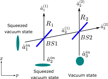
Figure 6: Generation of tripartite entanglement. Two squeezed modes $\hat{a}_{1}^{in}$, $\hat{a}_{2}^{in}$ are first combined using a beam splitter labelled $BS1$ that has a reflectivity $R_{1}^{2}$. One output of $BS1$ is subsequently combined with a third input $\hat{a}_{3}^{in}$ using a second beam splitter $BS2$. The three entangled output modes are $\hat{a}_{1}^{\left(1\right)}$, $\hat{a}_{2}^{\left(2\right)}$ and $\hat{a}_{3}^{\left(2\right)}$. The first input mode is squeezed in the $p$-quadrature, i.e. $\Delta^{2}\hat{p}_{1}^{in}=e^{-2r_{1}}$, while the second input mode is squeezed in the $x$-quadrature with $\Delta^{2}\hat{x}_{2}^{in}=e^{-2r_{2}}$, and the third input mode is a vacuum state. The generalization to $M$-partite entanglement is achieved by simply extending the above experimental configuration using $M-1$ beam splitters, as described in the main text.

Taking $R_{1}=R_{2}=\frac{1}{\sqrt{2}}$, from (37) we see that $\Delta^{2}(\hat{x}_{1}^{(1)}-\frac{1}{\sqrt{2}}(\hat{x}_{2}^{(2)}+\hat{x}_{3}^{(2)}))=2e^{-2r_{2}}$ and $\Delta^{2}(\hat{p}_{1}^{(1)}+\frac{1}{\sqrt{2}}(\hat{p}_{2}^{(2)}+\hat{p}_{3}^{(2)}))=2e^{-2r_{1}}$. These variances are both zero for large $r_{i}$, and the three output fields satisfy the condition

$$\Delta(\hat{x}_{1}^{(1)}-\frac{1}{\sqrt{2}}(\hat{x}_{2}^{(2)}+\hat{x}_{3}^{(2)}))\Delta(\hat{p}_{1}^{(1)}+\frac{1}{\sqrt{2}}(\hat{p}_{2}^{(2)}+\hat{p}_{3}^{(2)}))<1$$ (51)

known to certify genuine tripartite entanglement. This condition was proved to be sufficient for the verification of full tripartite inseparability in [76], and was proved sufficient to confirm genuine tripartite entanglement in [77]. The reader is referred to equation (17) of [77] with equal gains for the second and third modes. In fact, the product on the left side of the inequality becomes zero, indicating a maximum EPR entanglement, in the limit of large $r_{i}$.

The EPR paradox is seen to hold for $r_{1}$ and $r_{2}$ becoming large. The EPR correlations of the two-mode state are transferred directly onto the three modes. The paradox is observed because measurements can be made on the two fields $a_{2}$ and $a_{3}$ to give the value of $\frac{1}{\sqrt{2}}(\hat{x}_{2}^{(2)}+\hat{x}_{3}^{(2)})$, from which the outcome of $\hat{x}_{1}^{(1)}$ can be predicted with certainty. Similarly, the outcome of $\hat{p}_{1}^{(1)}$ can be predicted with certainty by measurement of $\frac{1}{\sqrt{2}}(\hat{p}_{2}^{(2)}+\hat{p}_{3}^{(2)})$. When the fields are spatially separated, the premise of local realism can be applied and the paradox follows. In fact, the condition (51) is seen to be the condition given by (46) for an EPR paradox. The condition is also a verification of the EPR steering of mode $1$, by measurements made on modes $2$ and $3$.

This leaves us to examine the EPR steering condition more carefully. On taking $R_{2}=\frac{1}{\sqrt{2}}$, from (45) we see on substituting (50),

$$\Delta^{2}(\hat{x}_{1}^{(1)}-\frac{g_{x}}{\sqrt{2}}(\hat{x}_{2}^{(2)}+\hat{x}_{3}^{(2)})) = \frac{2e^{-2r_{2}}}{1+e^{-2(r_{2}+r_{1})}}$$

$$\Delta^{2}(\hat{p}_{1}^{(1)}+\frac{g_{p}}{\sqrt{2}}(\hat{p}_{2}^{(2)}+\hat{p}_{3}^{(2)})) = \frac{2e^{-2r_{1}}}{1+e^{-2(r_{1}+r_{2})}}\,.$$ (52)

Hence the steering product defined for the three output modes is

$$S_{1|23}\equiv\Delta(\hat{x}_{1}^{(1)}-\frac{1}{\sqrt{2}}(\hat{x}_{2}^{(2)}+\hat{x}_{3}^{(2)}))\Delta(\hat{p}_{1}^{(1)}+\frac{1}{\sqrt{2}}(\hat{p}_{2}^{(2)}+\hat{p}_{3}^{(2)}))$$ (53)

which becomes

$$S_{1|23}=\frac{1}{\cosh(r_{1}+r_{2})}$$ (54)

as given by (47). There is steering of system $1$ for $r_{1}>0$ or $r_{2}>0$, or both. A single squeezed input is all that is required, in principle, although stronger steering is obtained for smaller variances which are better achieved with two squeezed input fields. Properties of genuine multipartite steering are studied elsewhere [64].

To generate four-partite entanglement where $M=4$, the process continues with another beam splitter, $BS3$.

$$\hat{a}_{3}^{(3)} = R_{3}\hat{a}_{3}^{(2)}+T_{3}\hat{a}_{4}^{in}$$

$$\hat{a}_{4}^{(3)} = T_{3}\hat{a}{}_{3}^{(2)}-R_{3}\hat{a}_{4}^{in}.$$ (55)

The output of mode $\hat{a}_{3}$ is denoted $\hat{a}_{3}^{(3)}$ and the output of mode $\hat{a}_{4}$ is denoted $\hat{a}_{4}^{(3)}$. For a suitable choice of $R_{3}$, the four outputs $a_{1}^{(1)}$, $a_{2}^{(2)}$, $a_{3}^{(3)}$and $a_{4}^{(3)}$ are genuinely $4$-partite entangled.

In fact, it is possible to continue the process of splitting the final field using a beam splitter, to create a system of $M$ output modes from a string of $M-1$ beam splitters. The reflectivities of the string of beam splitters can be selected so that the correlations are governed by the two-mode EPR correlations emerging from the first two beam splitters. For the $M$ modes given by outputs $a_{1}^{(1)}$, $a_{2}^{(2)}$, $a_{3}^{(3)}$, $..,a_{M-1}^{(M-1)}$, $a_{M}^{(M-1)}$, it follows that

$$\Delta^{2}(\hat{x}_{1}^{(1)}-\frac{1}{\sqrt{M-1}}(\hat{x}_{2}^{(2)}+\hat{x}_{3}^{(3)}+..\hat{x}_{M}^{(M-1)})) =2e^{-2r_{2}}$$

$$\Delta^{2}(\hat{p}_{1}+\frac{1}{\sqrt{M-1}}(\hat{p}_{2}^{(2)}+\hat{p}_{3}^{(3)}+..\hat{p}_{M}^{(M-1)})) =2e^{-2r_{1}},$$ (56)

which gives genuine $M$-partite entanglement. This is done by selecting for the beam splitters, $R_{M-1}^{2}=1/2$, $R_{M-2}^{2}=\frac{1}{3}$, $R_{M-j}^{2}=\frac{1}{j+1}$ for $j<M-1$, with $R_{1}^{2}=1/2$ [76, 77]. A criterion to confirm the detection of the genuine $M$-partite entanglement is defined in the next section.

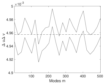
Figure 7: Simulation of multipartite entanglement in the Wigner representation, with two $r=3$ squeezed inputs. Sampling errors are indicated by the upper and lower error bars. Exact results are shown by the dashed line. In these simulations, there were 120 repeats of a 1000 sample parallel ensemble, to obtain sampling error estimates. Sampling errors are independent of the mode number, at about $\pm 10^{-5}.$

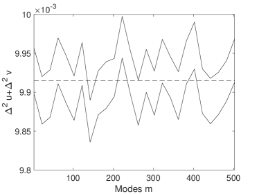
Figure 8: Simulation of multipartite entanglement in the Wigner representation, with two $r=3$ squeezed inputs. Sampling errors are indicated by the upper and lower error bars. Exact results are shown by the dashed line. In these simulations, there were 120 repeats of a 1000 sample parallel ensemble, to obtain sampling error estimates. Sampling errors are independent of the mode number, at about $\pm 2\times 10^{-5}.$

V.4 Detecting M-partite entanglement

Let $\hat{u}=\hat{x}_{1}-\frac{1}{\sqrt{M-1}}(\hat{x}_{2}+\hat{x}_{3}+..\hat{x}_{M})$ and $\hat{v}=\hat{p}_{1}+\frac{1}{\sqrt{M-1}}(\hat{p}_{2}+\hat{p}_{3}+..\hat{p}_{M})$ be the quadrature amplitudes as defined in the section above. Then the observation of

$$(\Delta\hat{u})(\Delta\hat{v})<\frac{2}{\left(M-1\right)}$$ (57)

confirms $M$-partite entanglement for all $M$. The observation of

$$(\Delta\hat{u})^{2}+(\Delta\hat{v})^{2}<\frac{4}{M-1}$$ (58)

also confirms $M$-partite entanglement for all $M$. The second result follows from the first, because if $\Delta^{2}u+\Delta^{2}v<\frac{4}{(N-1)}$, then it must be true that $\Delta u\Delta v<\frac{2}{M-1}$ (use $x^{2}+y^{2}\geq 2xy$). The second result was derived in [76] for the confirmation of full $M$-partite inseparability. Typical simulation results are shown in Figs (7) and (8), for $r=3$ inputs, showing complete agreement with analytic theory, up to the sampling error. Clearly, multimode entanglement is only confirmed for the product method at large $M$.

Clearly, the outputs of the above network satisfy this criterion for large enough $r_{i}$, with $\Delta u\Delta v=2e^{-(r_{1}+r_{2})}<\frac{2}{M-1}$. With $r_{1}=r_{2}$, we can detect the entanglement using this criterion for squeeze parameter $r>\frac{1}{2}ln(M-1)$. We mention that the criterion is sufficient but not necessary to detect the multipartite entanglement, and other methods are possible. This is especially true if one is justified to assume pure or Gaussian states, or is interested in determining only full multipartite inseparability. The reader is referred to [78, 79, 80, 81, 82, 83]. The above criterion however does not require these assumptions. The use of just one squeezed input will also generate an $M$-partite entangled state, for larger values of $r$. The use of more squeezed inputs allows generation of CV GHZ and cluster states that have an improved scaling for $M$ [76].

Proof: The proof follows that given in [76], but is modified to account for a product criterion, and to allow for mixed states. We follow the methods developed in [77]. Consider constants $g$ and $h$: Then for mixtures, it is always true [64] that

$$\Delta(u)\Delta(v) \geq \sum_{R}P_{R}\Delta_{R}u\Delta_{R}v$$ (59)

where $u=x_{1}-g(x_{2}+x_{3}+...+x_{M})$ and $v=p_{1}+h(p_{2}+p_{3}+..+p_{M})$. Here we assume $\rho=\sum_{R}P_{R}\rho_{R}$ where $\rho_{R}$ is a pure state, and $\sum_{R}P_{R}=1$ where $P_{R}>0$ is a probability. The $(\Delta_{R}u)^{2}$ denotes the variance of $u$ with respect to the pure state $R$.

To prove $M$-partite entanglement, one needs to prove entanglement across every bipartition. Consider a pure product state that is separable along bipartition $R-S$, where $R$ contains $M_{R}$ systems and $S$ contains $M_{S}$ systems, such that $M_{R}+M_{S}=M$. Then let $R$ contain system $1$, and we note that $M_{S}\geq 1$ and $M_{R}\geq 1$. Let the modes $1$, $i,..$ be elements of $R$ and the modes $j$, $k$,.. be elements of $S$. For a product state, as arises from pure separable systems $A$ and $B$, the variance of the sum of two observables $X_{A}+X_{B}$ will satisfy

$$(\Delta(X_{A}+X_{B}))^{2} = (\Delta X_{A})^{2}+(\Delta X_{B})^{2}$$ (60)

where here $X_{A}$ ($X_{B}$) is an observable for system $A$ ($B$). Therefore,

$$(\Delta u\Delta v)^{2} = \{(\Delta(x_{1}-gx_{i}+..)^{2}+(\Delta(gx_{j}+gx_{k}+..)^{2}\}$$ (61)

$$\times\{(\Delta(p_{1}+gp_{i}+.))^{2}+(\Delta(gp_{j}+gp_{k}+..)^{2}\}$$

$$\geq \{\Delta(x_{1}-gx_{i}+..)(\Delta(p_{1}+gp_{i}+..)$$

$$+(\Delta(gx_{j}+gx_{k}+..)(\Delta(gp_{j}+gp_{k}+..)\}^{2}$$

$$\geq (\frac{M_{s}}{M-1}+\frac{M_{s}}{M-1})^{2}$$

$$\geq \frac{4}{(M-1)^{2}}$$

where we have used $(a^{2}+b^{2})(c^{2}+d^{2})\geq(|ac|+|bd|)^{2}$, which is easily proved on noting that $(bc)^{2}+(ad)^{2}\geq 2|acbd|$. We have also used

$$\Pi_{1} \equiv \Delta(x_{1}-gx_{i}+..)\Delta(p_{1}+gp_{i}+..)$$

$$\geq \frac{1}{2}|\langle[x_{1}-gx_{i}+..,p_{1}+hp_{i}+..]\rangle|$$

$$\geq \frac{1}{2}|\langle[x_{1},p_{1}]-gh[x_{i},p_{i}]+..\rangle|$$

$$= 1-(M_{R}-1)gh$$

$$= 1-\frac{(M_{R}-1)}{M-1}$$

$$= \frac{M-M_{R}}{M-1}=\frac{M_{s}}{M-1}$$ (63)

and, similarly,

$$\Pi_{j} \equiv \Delta(x_{j}+x_{k}+..)\Delta(p_{j}+p_{k}+..)$$

$$\geq \frac{1}{2}|\langle[x_{j}+x_{k}+..,p_{j}+p_{k}+..]\rangle|$$

$$\geq \frac{1}{2}|\langle[x_{j},p_{j}]+[x_{k},p_{k}]+..\rangle|$$

$$= M_{S}\,.$$ (65)

This gives the required entanglement result, with a typical simulation result in Fig (7), using $r=3$ squeezed inputs. $\square$

All of these rather complex operations can be readily simulated using a simple unitary transformation on the amplitudes, and typical results for up to $500\times 500$ unitaries are given in Figs (7) and (8). However, in this case it is the Wigner representation that is the most efficient simulation technique, not the positive-P representation. This has a much larger sampling error, as shown in Fig (9). The reason for this is that the Wigner representation directly represents the symmetric operator ordering of the quadrature measurements. When there is a mismatch between the measurement ordering and the representation ordering, corrections are needed that increase the sampling error.

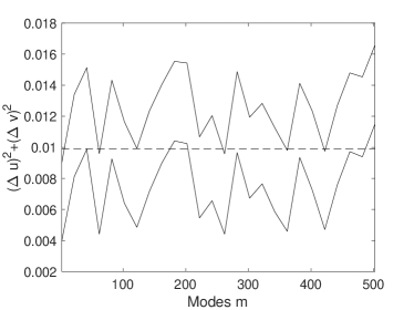
Figure 9: Simulation of multipartite entanglement in the positive-P representation, with two $r=3$ squeezed inputs. Sampling errors are indicated by the upper and lower error bars. Exact results are shown by the dashed line. In these simulations, there were 1200 repeats of a 2000 sample parallel ensemble, to obtain sampling error estimates. Sampling errors are independent of the mode number, at about $\pm 2\times 10^{-3}.$ Despite the $20\times$ larger ensemble, sampling errors are still two orders of magnitude larger than for the Wigner simulations given above.

VI Outlook

We have given a short tutorial account of recent developments in the use of phase-space simulations to treat large, linear networks. These methods can efficiently predict the moments and correlations of Gaussian boson samplers to all orders. This allows an assessment of whether such devices are in fact performing as expected theoretically. The addition of extra noise and decoherence as found experimentally can be easily included. In addition, it is possible to simulate the detection of a large variety of other nonclassical signatures, including multipartite EPR effects.

The focus here is on classical simulations that can verify measured correlations and probability distributions in linear networks. We find similar levels of complexity between the experiments and the verification simulations, meaning that the simulations themselves are reasonably fast. They are mostly limited by the Fourier transforms needed to bin the data in the GBS case.

However, this does not mean that the classical computer has really performed the same task in a similar time to the quantum experiment. Actually, for the generation of entangled states this is true, as the outputs are identical. For the GBS case, which is known to be a complex task, the simulations generate random complex numbers that allow verification of the GBS experimental data after binning, but they do not directly replicate the experimentally generated bits.

We also showed that while the positive-P method is well-suited to photon-counting and GBS verification, the Wigner method has lower sampling errors for simulating quadrature measurements, and multipartite entanglement. Nonlinear effects were not treated here. However, these are known to occur in such optical devices. It is not impossible to include them also, as previously demonstrated in nonlinear fiber-optical [84, 85] and BEC [86] systems. Nonlinearities are detrimental in the GBS case, but they are essential in other types of device such as the CIM [25].

While a tutorial of this type cannot cover all the recent developments, we also note two recent advances in theory [87] and experiment [88].

Acknowledgments

This work was funded through the Australian Research Council Discovery Project scheme under Grants DP180102470 and DP190101480, and through a research grant from NTT Research Corporation.

References

- Zhong et al. [2020] H.-S. Zhong, H. Wang, Y.-H. Deng, M.-C. Chen, L.-C. Peng, Y.-H. Luo, J. Qin, D. Wu, X. Ding, Y. Hu, et al., Science 370, 1460 (2020).
- Honjo et al. [2021] T. Honjo, T. Sonobe, K. Inaba, T. Inagaki, T. Ikuta, Y. Yamada, T. Kazama, K. Enbutsu, T. Umeki, R. Kasahara, et al., Science advances 7, eabh0952 (2021).
- Altland and Simons [2010] A. Altland and B. Simons, Condensed Matter Field Theory, second edition ed. (Cambridge University Press, 2010).
- Aaronson and Arkhipov [2013] S. Aaronson and A. Arkhipov, Theory of Computing 9, 143 (2013).
- Drummond et al. [2016] P. D. Drummond, B. Opanchuk, L. Rosales-Zárate, M. D. Reid, and P. J. Forrester, Physical Review A 94, 042339 (2016).
- Caves [1981] C. M. Caves, Physical Review D 23, 1693 (1981).
- McCuller et al. [2020] L. McCuller, C. Whittle, D. Ganapathy, K. Komori, M. Tse, A. Fernandez-Galiana, L. Barsotti, P. Fritschel, M. MacInnis, F. Matichard, K. Mason, N. Mavalvala, R. Mittleman, H. Yu, M. E. Zucker, and M. Evans, Physical Review Letters 124, 171102 (2020).
- Motes et al. [2015] K. R. Motes, J. P. Olson, E. J. Rabeaux, J. P. Dowling, S. J. Olson, and P. P. Rohde, Phys. Rev. Lett. 114, 170802 (2015).
- Olson et al. [2017] J. P. Olson, K. R. Motes, P. M. Birchall, N. M. Studer, M. LaBorde, T. Moulder, P. P. Rohde, and J. P. Dowling, Phys. Rev. A 96, 013810 (2017).
- Su et al. [2017] Z.-E. Su, Y. Li, P. P. Rohde, H.-L. Huang, X.-L. Wang, L. Li, N.-L. Liu, J. P. Dowling, C.-Y. Lu, and J.-W. Pan, Phys. Rev. Lett. 119, 080502 (2017).
- Boixo et al. [2018] S. Boixo, S. V. Isakov, V. N. Smelyanskiy, R. Babbush, N. Ding, Z. Jiang, M. J. Bremner, J. M. Martinis, and H. Neven, Nature Physics 14, 595 (2018).
- Aaronson and Arkhipov [2011] S. Aaronson and A. Arkhipov, in Proceedings of the 43rd Annual ACM Symposium on Theory of Computing (ACM Press, 2011) pp. 333–342.
- Marandi et al. [2014] A. Marandi, Z. Wang, K. Takata, R. L. Byer, and Y. Yamamoto, Nature Photonics 8, 937 (2014).
- Zhong et al. [2021a] H.-S. Zhong, Y.-H. Deng, J. Qin, H. Wang, M.-C. Chen, L.-C. Peng, Y.-H. Luo, D. Wu, S.-Q. Gong, H. Su, Y. Hu, P. Hu, X.-Y. Yang, W.-J. Zhang, H. Li, Y. Li, X. Jiang, L. Gan, G. Yang, L. You, Z. Wang, L. Li, N.-L. Liu, J. J. Renema, C.-Y. Lu, and J.-W. Pan, Phys. Rev. Lett. 127, 180502 (2021a), number of pages: 9 Publisher: American Physical Society.
- Aaronson [2011] S. Aaronson, Proceedings of the Royal Society of London A: Mathematical, Physical and Engineering Sciences 467, 3393 (2011).
- Yamamoto et al. [2017] Y. Yamamoto, K. Aihara, T. Leleu, K.-i. Kawarabayashi, S. Kako, M. Fejer, K. Inoue, and H. Takesue, npj Quantum Information 3, 1 (2017).
- Tanenbaum [1978] A. S. Tanenbaum, Communications of the ACM 21, 237 (1978).
- Neville et al. [2017] A. Neville, C. Sparrow, R. Clifford, E. Johnston, P. M. Birchall, A. Montanaro, and A. Laing, Nature Physics 13, 1153 (2017).
- Gupt et al. [2020] B. Gupt, J. M. Arrazola, N. Quesada, and T. R. Bromley, Quantum Information Processing 19, 1 (2020).
- Li et al. [2020] Y. Li, M. Chen, Y. Chen, H. Lu, L. Gan, C. Lu, J. Pan, H. Fu, and G. Yang, arXiv preprint arXiv:2009.01177 (2020).
- Quesada and Arrazola [2020] N. Quesada and J. M. Arrazola, Physical Review Research 2, 023005 (2020).
- Opanchuk et al. [2018] B. Opanchuk, L. Rosales-Zárate, M. D. Reid, and P. D. Drummond, Physical Review A 97, 042304 (2018).
- Drummond and Opanchuk [2020] P. D. Drummond and B. Opanchuk, Physical Review Research 2, 033304 (2020).
- Drummond et al. [2021] P. D. Drummond, B. Opanchuk, A. Dellios, and M. D. Reid, arXiv preprint arXiv:2102.10341 (2021).
- Kiesewetter and Drummond [2021] S. Kiesewetter and P. D. Drummond, arXiv preprint arXiv:2105.04190 (2021).
- Monroe [2020] D. Monroe, Communications of the ACM 64, 16 (2020).
- Schollwöck [2005] U. Schollwöck, Rev. Mod. Phys. 77, 259 (2005).
- Wigner [1932] E. Wigner, Physical Review 40, 749 (1932).
- Dirac [1945] P. A. M. Dirac, Rev. Mod. Phys. 17, 195 (1945).
- Moyal [1949] J. E. Moyal, Mathematical Proceedings of the Cambridge Philosophical Society 45, 99 (1949).
- Husimi [1940] K. Husimi, Proc. Phys. Math. Soc. Jpn. 22, 264 (1940).
- Schrödinger [1926] E. Schrödinger, Naturwissenschaften 14, 664 (1926).
- Glauber [1963a] R. J. Glauber, Phys. Rev. 131, 2766 (1963a).
- Cahill and Glauber [1969a] K. E. Cahill and R. J. Glauber, Phys. Rev. 177, 1882 (1969a).
- Drummond and Gardiner [1980] P. D. Drummond and C. W. Gardiner, Journal of Physics A: Mathematical and General 13, 2353 (1980).
- Drummond and Chaturvedi [2016] P. D. Drummond and S. Chaturvedi, Physica Scripta 91, 073007 (2016).
- Drummond and Hardman [1993] P. D. Drummond and A. D. Hardman, Europhys. Lett. 21, 279 (1993).
- Mari and Eisert [2012] A. Mari and J. Eisert, Physical review letters 109, 230503 (2012).
- Veitch et al. [2014] V. Veitch, S. H. Mousavian, D. Gottesman, and J. Emerson, New Journal of Physics 16, 013009 (2014).
- Cahill and Glauber [1969b] K. E. Cahill and R. J. Glauber, Physical Review 177, 1882 (1969b).
- Corney et al. [2008] J. F. Corney, J. Heersink, R. Dong, V. Josse, P. D. Drummond, G. Leuchs, and U. L. Andersen, Physical Review A 78, 023831 (2008).
- Bartlett et al. [2002] S. D. Bartlett, B. C. Sanders, S. L. Braunstein, and K. Nemoto, Physical Review Letters 88, 097904 (2002).
- Opanchuk et al. [2019] B. Opanchuk, L. Rosales-Zárate, M. D. Reid, and P. D. Drummond, Optics Letters 44, 343 (2019).
- Glauber [1963b] R. J. Glauber, Phys. Rev. 130, 2529 (1963b).
- Gardiner [2004] C. Gardiner, Handbook of Stochastic Methods for Physics, Chemistry, and the Natural Sciences, Springer complexity (Springer, 2004).
- Drummond and Hillery [2014] P. D. Drummond and M. Hillery, The quantum theory of nonlinear optics (Cambridge University Press, 2014).
- Hamilton et al. [2017] C. S. Hamilton, R. Kruse, L. Sansoni, S. Barkhofen, C. Silberhorn, and I. Jex, Phys. Rev. Lett. 119, 170501 (2017).
- Quesada et al. [2018] N. Quesada, J. M. Arrazola, and N. Killoran, Physical Review A 98, 062322 (2018).
- Bulmer et al. [2021] J. F. Bulmer, B. A. Bell, R. S. Chadwick, A. E. Jones, D. Moise, A. Rigazzi, J. Thorbecke, U.-U. Haus, T. Van Vaerenbergh, R. B. Patel, et al., arXiv preprint arXiv:2108.01622 (2021).
- Wu et al. [2018] J. Wu, Y. Liu, B. Zhang, X. Jin, Y. Wang, H. Wang, and X. Yang, National Science Review 5, 715 (2018).
- Boretti [2017] A. Boretti, The Future of the Internal Combustion Engine after “Diesel-Gate”, Tech. Rep. (SAE Technical Paper, 2017).
- Walschaers et al. [2016] M. Walschaers et al., New Journal of Physics 18, 032001 (2016).
- Phillips et al. [2019] D. Phillips, M. Walschaers, J. Renema, I. Walmsley, N. Treps, and J. Sperling, Physical Review A 99, 023836 (2019).
- Huang et al. [2017] H.-L. Huang, H.-S. Zhong, T. Li, F.-G. Li, X.-Q. Fu, S. Zhang, X. Wang, and W.-S. Bao, Scientific reports 7, 1 (2017).
- Moran [1984] P. A. P. Moran, An introduction to probability theory (Clarendon Press, Oxford, 1984).
- Chabaud et al. [2021] U. Chabaud, F. Grosshans, E. Kashefi, and D. Markham, Quantum 5, 578 (2021).
- Broome et al. [2013] M. A. Broome, A. Fedrizzi, S. Rahimi-Keshari, J. Dove, S. Aaronson, T. C. Ralph, and A. G. White, Science 339, 794 (2013).
- Spring et al. [2013] J. B. Spring, B. J. Metcalf, P. C. Humphreys, W. S. Kolthammer, X.-M. Jin, M. Barbieri, A. Datta, N. Thomas-Peter, N. K. Langford, D. Kundys, et al., Science 339, 798 (2013).
- Wang et al. [2019] H. Wang, J. Qin, X. Ding, M. C. Chen, S. Chen, X. You, Y. M. He, X. Jiang, L. You, Z. Wang, C. Schneider, J. J. Renema, S. Höfling, C.-Y. Lu, and J. W. Pan, Physical Review Letters 123, 250503 (2019).
- Fearn and Collett [1988] H. Fearn and M. Collett, Journal of Modern Optics 35, 553 (1988).
- Janszky and Vinogradov [1990] J. Janszky and A. V. Vinogradov, Physical review letters 64, 2771 (1990).
- Sperling et al. [2012] J. Sperling, W. Vogel, and G. S. Agarwal, Phys. Rev. A 85, 023820 (2012).
- Reid [1989] M. D. Reid, Phys. Rev. A 40, 913 (1989).
- Teh et al. [2021] R. Y. Teh, M. Gessner, M. D. Reid, and M. Fadel, arXiv preprint arXiv:2108.06926 (2021).
- Einstein et al. [1935] A. Einstein, B. Podolsky, and N. Rosen, Phys. Rev. 47, 777 (1935).
- Giovannetti et al. [2003] V. Giovannetti, S. Mancini, D. Vitali, and P. Tombesi, Physical Review A 67, 022320 (2003).
- Cavalcanti et al. [2009] E. G. Cavalcanti, S. Jones, H. M. Wiseman, and M. D. Reid, Phys. Rev. A 80, 032112 (2009).
- Wiseman et al. [2007] H. M. Wiseman, S. J. Jones, and A. C. Doherty, Phys. Rev. Lett. 98, 140402 (2007).
- Branciard et al. [2012] C. Branciard, E. G. Cavalcanti, S. P. Walborn, V. Scarani, and H. M. Wiseman, Phys. Rev. A 85, 010301 (2012).
- Opanchuk et al. [2014] B. Opanchuk, L. Arnaud, and M. D. Reid, Phys. Rev. A 89, 062101 (2014).
- Uola et al. [2020] R. Uola, A. C. S. Costa, H. C. Nguyen, and O. Gühne, Rev. Mod. Phys. 92, 015001 (2020).
- Rosales-Zárate et al. [2015] L. Rosales-Zárate, R. Y. Teh, S. Kiesewetter, A. Brolis, K. Ng, and M. D. Reid, JOSA B 32, A82 (2015).
- Reid et al. [2009] M. D. Reid, P. D. Drummond, W. P. Bowen, E. G. Cavalcanti, P. K. Lam, H. A. Bachor, U. L. Andersen, and G. Leuchs, Rev. Mod. Phys. 81, 1727 (2009).
- He and Reid [2013] Q. He and M. Reid, Physical Review A 88, 052121 (2013).
- Kiesewetter et al. [2014] S. Kiesewetter, Q. Y. He, P. D. Drummond, and M. D. Reid, Phys. Rev. A 90, 043805 (2014).
- van Loock and Furusawa [2003] P. van Loock and A. Furusawa, Physical Review A 67, 052315 (2003).
- Teh and Reid [2014] R. Y. Teh and M. D. Reid, Physical Review A 90, 062337 (2014).
- Sperling and Vogel [2013] J. Sperling and W. Vogel, Physical review letters 111, 110503 (2013).
- Gerke et al. [2015] S. Gerke, J. Sperling, W. Vogel, Y. Cai, J. Roslund, N. Treps, and C. Fabre, Physical review letters 114, 050501 (2015).
- Villar et al. [2005] A. S. Villar, L. S. Cruz, K. N. Cassemiro, M. Martinelli, and P. Nussenzveig, Physical Review Letters 95, 243603 (2005).
- Chen et al. [2014] M. Chen, N. C. Menicucci, and O. Pfister, Phys. Rev. Lett. 112, 120505 (2014).
- Coelho et al. [2009] A. Coelho, F. Barbosa, K. Cassemiro, A. Villar, M. Martinelli, and P. Nussenzveig, Science 326, 823 (2009).
- Shalm et al. [2013] L. K. Shalm, D. R. Hamel, Z. Yan, C. Simon, K. J. Resch, and T. Jennewein, Nature Physics 9, 19 (2013).
- Drummond et al. [1981] P. D. Drummond, C. W. Gardiner, and D. F. Walls, Phys. Rev. A 24, 914 (1981).
- Carter et al. [1987] S. J. Carter, P. D. Drummond, M. D. Reid, and R. M. Shelby, Physical Review Letters 58, 1841 (1987).
- Deuar and Drummond [2007] P. Deuar and P. D. Drummond, Phys. Rev. Lett. 98, 120402 (2007).
- Villalonga et al. [2021] B. Villalonga, M. Y. Niu, L. Li, H. Neven, J. C. Platt, V. N. Smelyanskiy, and S. Boixo, arXiv preprint arXiv:2109.11525 (2021).
- Zhong et al. [2021b] H.-S. Zhong, Y.-H. Deng, J. Qin, H. Wang, M.-C. Chen, L.-C. Peng, Y.-H. Luo, D. Wu, S.-Q. Gong, H. Su, et al., Physical review letters 127, 180502 (2021b).