Toeplitz Least Squares Problems,
Fast Algorithms and Big Data

Abstract

In time series analysis, when fitting an autoregressive model, one must solve a Toeplitz ordinary least squares problem numerous times to find an appropriate model, which can severely affect computational times with large data sets. Two recent algorithms (LSAR and Repeated Halving) have applied randomized numerical linear algebra (RandNLA) techniques to fitting an autoregressive model to big time-series data. We investigate and compare the quality of these two approximation algorithms on large-scale synthetic and real-world data. While both algorithms display comparable results for synthetic datasets, the LSAR algorithm appears to be more robust when applied to real-world time series data. We conclude that RandNLA is effective in the context of big-data time series.

1 Introduction

Advancements in technology and computation have led to enormous data sets being generated from various fields of research including science, internet datasets and business. These data sets, commonly described as Big Data, are stored in the form of vectors and matrices, allowing us to draw on our knowledge of linear algebra to analyze them. The enormity of Big Data matrices has mandated the search for large-scale matrix algorithms with improved run times and stability [8].

Randomised Numerical Linear Algebra (RandNLA) is a new tool to deal with big data [24]. RandNLA utilises random sampling of elements, rows, or columns of a matrix to produce a second smaller matrix that is similar to the first matrix in some way, yet computationally easier to deal with (e.g., [8, 7, 9, 5, 27]). An application of RandNLA is in finding fast solutions for Toeplitz least squares problems (e.g., [17, 25]).

Toeplitz matrices and Toeplitz least squares problems occur in many practical large-scale matrix problems such as time series analysis and signal/image processing [8, 17]. In practice they can become a computational bottleneck. In the context of stochastic dynamic systems, autoregressive models require the solutions of many ordinary least squares problems with Toeplitz structure [16]. Such stochastic dynamic models have a wide range of applications, from supply chains [18, 19, 20, 1] and energy systems (e.g., [15, 14]) to epidemiology [3, 4, 11, 10]) and computational complexity (e.g., [12, 2, 13]).

Recently, by utilising the particular structure of Toeplitz matrices and methods from RandNLA, some superfast algorithms have been developed for approximating Toeplitz linear least squares solutions (e.g., [17, 25]). We aim to compare the efficacy of these new algorithms on large-scale synthetic as well as real-world data.

Notation.

Vectors and matrices are denoted by bold lower-case and bold upper-case letters respectively (e.g., ${\bm{v}}$ and ${\bm{V}}$). Vectors are assumed to be column vectors. We use lower-case letters or Greek letters to denote scalar constants (e.g., $d$, $\epsilon$). Random variables are denoted by upper-case letters (e.g., $Y$). For a real vector ${\bm{v}}$, its transpose is ${\bm{v}}^{{\mathchoice{\raisebox{0.0pt}{$\displaystyle\intercal$}}{\raisebox{0.0pt}{$\textstyle\intercal$}}{\raisebox{0.0pt}{$\scriptstyle\intercal$}}{\raisebox{0.0pt}{$\scriptscriptstyle\intercal$}}}}$. For two vectors ${\bm{v}},{\bm{w}}$, their inner-product is $\left\langle{\bm{v}},{\bm{w}}\right\rangle={\bm{v}}^{{\mathchoice{\raisebox{0.0pt}{$\displaystyle\intercal$}}{\raisebox{0.0pt}{$\textstyle\intercal$}}{\raisebox{0.0pt}{$\scriptstyle\intercal$}}{\raisebox{0.0pt}{$\scriptscriptstyle\intercal$}}}}{\bm{w}}$. For a vector ${\bm{v}}$ and matrix ${\bm{V}}$, $\|{\bm{v}}\|$ and $\|{\bm{V}}\|$ denote the vector $\ell_{2}$ norm and matrix spectral norm. Adopting Matlab notation, we use ${\bm{A}}(i,:)$ to mean the $i\textsuperscript{th}$ row of ${\bm{A}}$, but we consider it as a column vector. Finally, ${\bm{e}}_{i}$ denotes a vector whose $i\textsuperscript{th}$ component is one, and zero elsewhere.

2 Ordinary Least Squares Problems

Suppose we have a system of linear equations ${\bm{A}}{\bm{x}}={\bm{b}}$ such that ${\bm{A}}\in{\rm I\!R}^{n\times d}$, ${\bm{x}}\in{\rm I\!R}^{d}$, ${\bm{b}}\in{\rm I\!R}^{n}$, and the system is strongly overdetermined ($n\gg d$), so that ${\bm{A}}$ is a tall and thin matrix. In general, ${\bm{A}}{\bm{x}}={\bm{b}}$ will be infeasible, meaning we may not be able to find an ${\bm{x}}$ that satisfies the equation. However, in many applications, it is of interest to find an${\bm{x}}^{\star}$ that minimizes the difference between ${\bm{A}}{\bm{x}}^{\star}$ and ${\bm{b}}$. The method of Ordinary Least Squares achieves this by minimising the sum of squares of the residual vector ${\bm{r}}={\bm{b}}-{\bm{A}}{\bm{x}}$. To formalise this, we define Ordinary Least Squares problems as follows.

[Ordinary Least Squares Problem] An Ordinary Least Squares (OLS) problem with inputs ${\bm{A}}{\in{\rm I\!R}^{n\times d}}$ and ${\bm{b}}\in{\rm I\!R}^{d}$ solves the minimisation problem

$$\min_{{\bm{x}}\in{\rm I\!R}^{d}}\|{\bm{A}}{\bm{x}}-{\bm{b}}\|^{2}.$$

The solution to this minimisation problem is well known and shown in Section 2 [17].

[Solution to OLS problem] The optimal solution of the OLS minimisation problem in Section 2 satisfies the normal equation

$${\bm{A}}^{{\mathchoice{\raisebox{0.0pt}{$\displaystyle\intercal$}}{\raisebox{0.0pt}{$\textstyle\intercal$}}{\raisebox{0.0pt}{$\scriptstyle\intercal$}}{\raisebox{0.0pt}{$\scriptscriptstyle\intercal$}}}}{\bm{A}}{\bm{x}}^{\star}={\bm{A}}^{{\mathchoice{\raisebox{0.0pt}{$\displaystyle\intercal$}}{\raisebox{0.0pt}{$\textstyle\intercal$}}{\raisebox{0.0pt}{$\scriptstyle\intercal$}}{\raisebox{0.0pt}{$\scriptscriptstyle\intercal$}}}}{\bm{b}},$$

which always has a solution. If ${\bm{A}}^{{\mathchoice{\raisebox{0.0pt}{$\displaystyle\intercal$}}{\raisebox{0.0pt}{$\textstyle\intercal$}}{\raisebox{0.0pt}{$\scriptstyle\intercal$}}{\raisebox{0.0pt}{$\scriptscriptstyle\intercal$}}}}{\bm{A}}$ is nonsingular, ${\bm{x}}^{\star}$ is unique. Otherwise, the unique solution of minimum norm $\|{\bm{x}}^{\star}\|$ can be found via the singular value decomposition of ${\bm{A}}$.

2.1 Solving Large OLS Problems via RandNLA

Randomised Numerical Linear Algebra (RandNLA) is a new tool to deal with big data. It utilises random sampling of the elements or rows or columns of a matrix to produce a second smaller (compressed) matrix that is similar to the first matrix in some way, yet computationally easier to deal with [9].

In this section we look at the application of RandNLA to OLS regression. We consider again the system of linear equations ${\bm{A}}{\bm{x}}={\bm{b}}$ with ${\bm{A}}\in{\rm I\!R}^{n\times d},{\bm{x}}\in{\rm I\!R}^{d}$, ${\bm{b}}\in{\rm I\!R}^{n}$ and $n>d$. In essence, RandNLA methods for OLS problems involve the appropriate choice of matrix ${\bm{S}}\in{\rm I\!R}^{c\times n}$ to perform some form of sampling (according to a chosen distribution) and/or pre-processing operation. We are able to compress our data matrix ${\bm{A}}\in{\rm I\!R}^{n\times d}$ into a smaller matrix ${\bm{S}}{\bm{A}}\in{\rm I\!R}^{c\times d}$ that will ideally lead to similar results. We replace the OLS problem (Section 2) by a compressed least squares approximation problem [27]

$$\min_{{\bm{x}}\in{\rm I\!R}^{d}}\|({\bm{S}}{\bm{A}}{\bm{x}})-({\bm{S}}{\bm{b}})\|^{2}.$$ (1)

A solution ${\bm{x}}^{\star}_{s}$ to the smaller problem 1 can be found using a direct method such as QR factorization of the matrix ${\bm{S}}{\bm{A}}$, giving an approximation to ${\bm{x}}^{\star}$ such that

$$\|{\bm{A}}{\bm{x}}^{\star}_{s}-{\bm{b}}\|\leq(1+\varepsilon)\|{\bm{A}}{\bm{x}}^{\star}-{\bm{b}}\|,$$ (2)

where $\varepsilon>0$. Since we have a randomised algorithm, there is some probability $\delta<1$ (depending on $\varepsilon>0$) with which the algorithm will fail, i.e., 2 will not be satisfied.

As mentioned, RandNLA methods for OLS problems depend on the choice of ${\bm{S}}$. One may argue that the simplest choice for ${\bm{S}}$ performs uniform random sampling on the rows of ${\bm{A}}$[17]. Unfortunately, while this can be achieved quite easily and quickly, uniform sampling strategies perform poorly because of nonuniformity in the rows of ${\bm{A}}$.

There are two ways to address this problem [27]. A data-independent (or data-oblivious) approach, such as Algorithm 1, involves some kind of preprocessing (or preconditioning) of matrix ${\bm{A}}$ that transforms it in order to make it more uniform. Random sampling can then be applied to this uniform, transformed ${\bm{A}}$. A second data-aware approach (such as using leverage scores) involves weighting the rows of ${\bm{A}}$ so that rows with more information, in some sense, are randomly sampled with higher probability.

2.1.1 Data-oblivious Approach: Sampled Randomised Hadamard Transform

Drineas and Mahoney [9] present a data-oblivious method for OLS called Sampled Randomised Hadamard Transform (SRHT). As discussed, a data-oblivious method overcomes nonuniformity in the rows of ${\bm{A}}$ by preprocessing ${\bm{A}}$ in some way. The Randomised Hadamard Transform (RHT) ${\bm{H}}_{m}{\bm{D}}$ performs this role. This is the product of ${\bm{H}}_{m}\in{\rm I\!R}^{n\times n}$ (defined in Section 2.1.1) and the diagonal matrix ${\bm{D}}\in{\rm I\!R}^{n\times n}$ with ${\bm{D}}_{ii}$ equal to 1 or $-1$ with probability $\frac{1}{2}$. Using the RHT to uniformise ${\bm{A}}$ has the advantage of being quite fast: $\mathcal{O}\left(n\log_{2}n\right)$ time to compute a vector ${\bm{H}}_{m}{\bm{D}}{\bm{x}}$, or $\mathcal{O}\left(n\log_{2}c\right)$ if we only want to access $c$ elements of vector ${\bm{H}}_{m}{\bm{D}}{\bm{x}}$ (as we do when sampling).

[Hadamard Transform] For some $m>0$, the Hadamard transform (normalised), denoted ${\bm{H}}_{m}\in{\rm I\!R}^{n\times n}$, $n=2^{m+1}$, is defined recursively with ${\bm{H}}_{0}=1$ and

$${\bm{H}}_{m}=\frac{1}{\sqrt{2}}\begin{pmatrix}{\bm{H}}_{m-1}&{\bm{H}}_{m-1}\\ {\bm{H}}_{m-1}&-{\bm{H}}_{m-1}\end{pmatrix}.$$

Following preprocessing, a uniform sampling matrix ${\bm{S}}\in{\rm I\!R}^{c\times n}$ is applied. This matrix is given in the sampling-and-rescaling form, but it may be implemented implicitly in practice through simply sampling the rows. Thus, when sampling and preprocessing are applied, we arrive at a smaller OLS problem

$$\min_{{\bm{x}}\in{\rm I\!R}^{d}}\|({\bm{S}}{\bm{H}}_{m}{\bm{D}}{\bm{A}}{\bm{x}})-({\bm{S}}{\bm{H}}_{m}{\bm{D}}{\bm{b}})\|^{2}.$$ (3)

[Number of Rows to Sample in SRHT Algorithm [9]] Let $x_{s}^{*}$ be an optimal solution to 3. If the ideal number of sampled rows is given by

$$c=\max{\Big{(}48^{2}d\ln{(40nd)}\ln{\big{(}100^{2}d\ln{(40nd)}\big{)}},40d\ln{\big{(}40nd\big{)}/\varepsilon}\Big{)}},$$ (4)

then for some $0<\varepsilon<1$, $\hbox{\bf{Pr}}(\|{\bm{A}}{\bm{x}}^{\star}_{s}-{\bm{b}}\|\leq(1+\varepsilon)\|{\bm{A}}{\bm{x}}^{\star}-{\bm{b}}\|)\geq 0.8$. Section 2.1.1 ensures that ${\bm{x}}^{\star}_{s}$ satisfies 2 with probability at least 0.8. The SRHT algorithm is described in Algorithm 1.

0:  ${\bm{A}}\in{\rm I\!R}^{n\times d}$, ${\bm{b}}\in{\rm I\!R}^{n}$, error parameter $\varepsilon\in(0,1)$

1:  Let $c$ be given by 4;

2:  Let ${\bm{S}}$ be an empty matrix;

3:  for $t=1,\dots,c$ (i.i.d. trials with replacement) do

4:     Select uniformly $i$ at random an integer from ${1,2,\dots,n}$;

5:     Append the row vector $(\sqrt{n/c}){\bm{e}}_{i}^{\mathchoice{\raisebox{0.0pt}{$\displaystyle\intercal$}}{\raisebox{0.0pt}{$\textstyle\intercal$}}{\raisebox{0.0pt}{$\scriptstyle\intercal$}}{\raisebox{0.0pt}{$\scriptscriptstyle\intercal$}}}$ to ${\bm{S}}$.

6:  end for

7:  Let ${\bm{H}}_{m}\in{\rm I\!R}^{n\times n}$ be the normalised Hadamard transform matrix;

8:  Let ${\bm{D}}\in{\rm I\!R}^{n\times n}$ be a diagonal matrix with

$${\bm{D}}_{ii}=\begin{cases}+1,&\text{with probability}\frac{1}{2};\\ -1,&\text{with probability}\frac{1}{2};\\ \end{cases}$$

8:  ${\bm{x}}^{\star}_{s}$, the solution of the OLS problem $\min_{{\bm{x}}_{s}\in{\rm I\!R}^{d}}\|\big{(}{\bm{S}}{\bm{H}}_{m}{\bm{D}}{\bm{A}}\big{)}{\bm{x}}_{s}-({\bm{S}}{\bm{H}}_{m}{\bm{D}}){\bm{b}}\|^{2}$.

Algorithm 1 SRHT Algorithm [9]

2.1.2 Data-aware Approach: Leverage Scores-based Random Sampling

As discussed in Section 2.1, an alternative to the data-oblivious approach is data-aware approaches, in which information from the data matrix is assessed before sampling to determine which rows are deemed (in some sense) more important and thus more ideal to be selected in the sampling procedure. In particular, leverage score sampling is a common way to assess the importance of a row. In general terms, a statistical leverage score measures how far the values of an observation are from other observations. Section 2.1.2 presents a more precise definition of leverage scores. [Leverage Score] Given matrix ${\bm{A}}\in{\rm I\!R}^{n\times d}$ with $n\geq d$ and $\text{rank}({\bm{A}})=d$, the $i$^th leverage score corresponding to the $i$^th row of ${\bm{A}}$ is given by the $i$^th diagonal entry of ${\bm{A}}({\bm{A}}^{{\mathchoice{\raisebox{0.0pt}{$\displaystyle\intercal$}}{\raisebox{0.0pt}{$\textstyle\intercal$}}{\raisebox{0.0pt}{$\scriptstyle\intercal$}}{\raisebox{0.0pt}{$\scriptscriptstyle\intercal$}}}}{\bm{A}})^{-1}{\bm{A}}^{{\mathchoice{\raisebox{0.0pt}{$\displaystyle\intercal$}}{\raisebox{0.0pt}{$\textstyle\intercal$}}{\raisebox{0.0pt}{$\scriptstyle\intercal$}}{\raisebox{0.0pt}{$\scriptscriptstyle\intercal$}}}}$; that is,

$$\ell(i) ={\bm{e}}_{i}^{{\mathchoice{\raisebox{0.0pt}{$\displaystyle\intercal$}}{\raisebox{0.0pt}{$\textstyle\intercal$}}{\raisebox{0.0pt}{$\scriptstyle\intercal$}}{\raisebox{0.0pt}{$\scriptscriptstyle\intercal$}}}}{\bm{A}}({\bm{A}}^{{\mathchoice{\raisebox{0.0pt}{$\displaystyle\intercal$}}{\raisebox{0.0pt}{$\textstyle\intercal$}}{\raisebox{0.0pt}{$\scriptstyle\intercal$}}{\raisebox{0.0pt}{$\scriptscriptstyle\intercal$}}}}{\bm{A}})^{-1}{\bm{A}}^{{\mathchoice{\raisebox{0.0pt}{$\displaystyle\intercal$}}{\raisebox{0.0pt}{$\textstyle\intercal$}}{\raisebox{0.0pt}{$\scriptstyle\intercal$}}{\raisebox{0.0pt}{$\scriptscriptstyle\intercal$}}}}{\bm{e}}_{i}~{}~{}\text{for}~{}~{}i=1,\dots,n.$$ (5)

It can be shown that $\ell(i)\geq 0$ for all $i$ and $\sum_{i=1}^{m}\ell(i)=d$, and so we can construct a probability distribution $\pi$ over the rows of ${\bm{A}}$ by

$$\pi(i):=\frac{\ell(i)}{d}~{}~{}\text{for}~{}~{}i=1,\dots,m.$$ (6)

Sampling according to leverage scores thus involves randomly selecting and rescaling rows of ${\bm{A}}$ proportional to their leverage scores. In terms of our sampling and rescaling formalism 1, ${\bm{S}}\in{\rm I\!R}^{c\times n}$ is constructed by randomly choosing each row (with replacement) from the $n\times n$ identity matrix according to the nonuniform distribution 6. If row $i$ is selected, it is rescaled by multiplying by $1/\sqrt{c\pi(i)}$. A Leverage-Score-Based Random Sampling algorithm is given in Algorithm 2.

0:  ${\bm{A}}\in{\rm I\!R}^{n\times d}$, ${\bm{b}}\in{\rm I\!R}^{n}$, error parameter $\varepsilon\in(0,1)$;

1:  Compute leverage scores $\ell(i)$ for $i=1,\dots,n$ as in Section 2.1.2;

2:  Compute the sampling distribution $\pi(i)$ for $i=1,\dots,n$ as in 6;

3:  Set $c$ as in 11;

4:  Form ${\bm{S}}\in{\rm I\!R}^{c\times n}$ by randomly choosing $c$ rows of the corresponding identity matrix according to the probability distribution $\pi$ with replacement and rescaling factor $\frac{1}{\sqrt{c\pi(i)}}$;

5:  Construct the sampled data matrix $\widehat{\bm{A}}={\bm{S}}{\bm{A}}$ and response vector $\widehat{\bm{b}}={\bm{S}}{\bm{b}}$;

6:  Solve the associated compressed OLS problems as in 1 using a conventional method;

6:  ${\bm{x}}^{\star}_{s}$, the solution of $\min_{{\bm{x}}\in{\rm I\!R}^{d}}\|\widehat{\bm{A}}{\bm{x}}-\widehat{\bm{b}}\|$.

Algorithm 2 Leverage Score Based Random Sampling

Computing leverage scores as in Section 2.1.2 is more costly than solving the original OLS problem. However, as we see in the coming section, one can find approximate leverage scores cheaply. The LSAR algorithm [17] utilises approximate leverage scores, and the REPEATEDHALVING [25] algorithm utilises generalised leverage scores with respect to a smaller approximate matrix. The downside of approximate leverage scores is that they mis-estimate the true leverage scores by some factor $0<\beta\leq 1$, that is $\widehat{\ell}(i)\geq\beta\ell(i),\text{ for }i=1,\dots,m$. This leads to a trade-off between speed and accuracy.

3 Toeplitz OLS Problems for Time-series Data

A Toeplitz Ordinary Least Squares (TOLS) problem is an OLS problem

$$\min_{x\in{\rm I\!R}^{d}}{\bm{z}}({\bm{x}})=\|\bm{T}{\bm{x}}-{\bm{b}}\|^{2}$$ (7)

in which $\bm{T}$ is a Toeplitz matrix as given in Section 3. As we can see, there are only $n+p-1$ distinct numbers. This is useful for computation and storage of Toeplitz matrices.

Motivation.

Toeplitz matrices arise in a wide range of problems in both pure mathematics (such as algebra, combinatorics, differential geometry, etc.) and applied mathematics (approximation theory, image processing, time series analysis, etc.)  [29]. In particular, fitting an AR$(p)$ model (see Section 3) to time series data requires solving a TOLS problem for multiple possible orders of $p$. Given the present ubiquity of data, one is often required to fit an AR model to very large time series data sets, referred to as big time-series data. This TOLS problem quickly becomes a computational bottleneck because of the need to solve 7 repeatedly for different values of $p$. However, by utilising the unique structure of Toeplitz matrices and methods from RandNLA, some superfast (i.e., faster than $O(np)$) algorithms have been developed recently for approximating solutions to TOLS problems. In the following sections we examine some of these algorithms.

[Toeplitz Matrix] A Toeplitz matrix has the form

$$\bm{T} =\begin{pmatrix}a_{p}&a_{p-1}&\dots&a_{1}\\ a_{p+1}&a_{p}&\ddots&a_{2}\\ \vdots&\ddots&\ddots&\vdots\\ a_{2p-1}&a_{2p-2}&\dots&a_{p}\\ \vdots&\vdots&\vdots&\vdots\\ a_{n+p-1}&a_{n+p-2}&\dots&a_{n}\\ \end{pmatrix},$$

where $a_{i}\in{\rm I\!R}$ for all $i$. It has constant descending diagonals.

A time series can be defined as a collection of random variables $\{Y_{t};~{}~{}t=0,\pm 1,\pm 2,\dots\}$ indexed according to time $t$. A time series is stationary (weakly stationary) if it has a constant mean $\mu$ that does not depend on $t$, and the autocovariance function $\text{Cov}(Y_{t},T_{t+h})$ depends only on lag $h=|s-t|$, the difference between two time points.

If the current value $Y_{t}$ can be explained with a function of $p$ past values, we can model the time series with an $\texttt{AR}(p)$ model.

[Autoregressive Model of Order $p$] An autoregressive model of order $p$, denoted AR$(p)$, has the form

$$Y_{t}=\phi_{1}Y_{t-1}+\phi_{2}Y_{t-2}+\dots+\phi_{p}Y_{t-p}+\mathcal{W}_{t},$$

where $Y_{t}$ is a stationary time series with mean zero, $\phi_{1},\phi_{2},\dots,\phi_{p}$ are the regression parameters with $\phi_{p}\neq 0$, and $\mathcal{W}_{t}$ is a Gaussian white noise series, i.e., each $\mathcal{W}_{t}$ is an independent and identically distributed normal random with mean 0 and variance $\sigma_{\mathcal{W}}^{2}$.

Given a set of time series observations $y_{1},\dots,y_{n}$, if we wish to fit an $\texttt{AR}(p)$ model, we need to find auto-regression parameters $\phi_{1},\phi_{2},\dots,\phi_{p}$. Finding these parameters exactly by the method of maximum likelihood estimates (i.e., by maximising the log-likelihood function) can be shown to be intractable and must be solved numerically [21]. However, finding the log-likelihood function of the parameters conditional (CMLE) on the first $p$ observations is an alternative approach for large samples, equivalent to obtaining the parameters from an OLS problem that regresses $y_{t}$ on $p$ of its own lagged values [21].

Parameters $\phi_{1},\phi_{2},\dots,\phi_{p}$ in the $\texttt{AR}(p)$ model $Y_{t}=\phi_{1}Y_{t-1}+\phi_{2}Y_{t-2}+\dots+\phi_{p}Y_{t-p}+\mathcal{W}_{t}$ are found by solving the OLS problem

$$\begin{pmatrix}y_{p+1}\\ y_{p+2}\\ \vdots\\ y_{n}\end{pmatrix} \approx\begin{pmatrix}y_{p}&y_{p-1}&\dots&y_{1}\\ y_{p+1}&y_{p}&\dots&y_{2}\\ \vdots&\vdots&\dots&\vdots\\ y_{n-1}&y_{n-2}&\dots&y_{n-p}\\ \end{pmatrix}\begin{pmatrix}\phi_{1}\\ \phi_{2}\\ \vdots\\ \phi_{p}\end{pmatrix},$$ (8a)

$${\bm{y}}_{n-p,1} \approx{\bm{X}}_{n-p,p}\bm{\phi}_{p,1},$$ (8b)

where ${\bm{X}}_{n,p}$ is a Toeplitz matrix, often referred to as the data matrix. Thus we arrive at a TOLS problem, where the order $p$ is an unknown parameter that must be estimated, typically using the partial autocorrelation function (PACF). [Partial Autocorrelation Function] The PACF of a stationary time series $\{Y_{t};~{}t=0,\pm 1,\pm 2,...\}$ at lag h is defined by

$$\begin{cases}\rho(Y_{t},Y_{t+1})&\text{for }h=1,\\ \rho(Y_{t}-\widehat{Y}_{t},Y_{t}-\widehat{Y}_{t,h})&\text{for }h\geq 2,\end{cases}$$ (9)

where $\rho$ denotes the correlation function and $\widehat{Y}_{t}$ and $\widehat{Y}_{t+h}$ are the linear regression of $Y_{t}$ and $Y_{t+h}$ on $\{X_{t+1},\dots,X_{t+h-1}\}$.

Order $p$ is estimated by selecting the last lag at which the PACF is nonzero. In the algorithm, $\tau_{h}$ denotes the PACF value estimated at lag $h$ using the CMLE of the parameters $\phi_{1},\phi_{2},\dots,\phi_{p}$ (i.e., through solving the associated TOLS problem). Also, $\widehat{\tau}_{h}$ denotes the PACF value using the CMLE of the parameters when based on the compressed (sampled and re-scaled) OLS problem.

Estimating the order $p$ requires solving the TOLS regression problem 7 multiple times with different $p$. In the context of big time-series data, these TOLS problems are the computational bottleneck.

3.1 LSAR Algorithm

Eshragh et al. [17] develop a fast algorithm called LSAR for estimating the leverage scores of an autoregressive model in big time-series data. To mitigate the computational complexity of solving numerous OLS problems, LSAR utilises a data-aware RandNLA sampling routine based on leverage scores. In this section we discuss how LSAR relates to Toeplitz OLS problems and then how to perform the algorithm.

As stated in Section 2.1.2, calculating leverage scores exactly could be computationally costly. However, Eshragh et al. [17] developed an efficient approximation to estimate the leverage scores recursively, as presented in 10.

[Approximate Leverage Scores] For an AR(p) model with $$p\geq 1$$, the fully-approximate leverage scores are given by the recursion

$$\widehat{\ell}_{n,p}(i):=\begin{cases}{\ell}_{n,1}(i)&\text{for }p=1,\\ \tilde{\ell}_{n,2}(i),&\text{for }p=2,\\ \widehat{\ell}_{n-1,p-1}(i)+\frac{(\widehat{\bm{r}}_{n-1,p-1}(i))^{2}}{\|\widehat{\bm{r}}_{n-1,p-1}\|^{2}},&\text{for }p\geq 3,\end{cases}$$ (10a)

where

$$\widehat{\bm{r}}_{n-1,p-1} :={\bm{X}}_{n-1,p-1}\widehat{\bm{\phi}}_{n-1,p-1}-{\bm{y}}_{n-1,p-1},$$ (10b)

and $$\widehat{\bm{\phi}}_{n-1,p-1} \widehat{\bm{X}}_{n-1,p-1}\in{\rm I\!R}^{c\times(p-1)} \widehat{\bm{y}}_{n-1,p-1}\in{\rm I\!R}^{c} \widehat{\bm{X}}_{n-1,p-1} \widehat{\bm{y}}_{n-1,p-1}$$ is the solution of the OLS problem with inputs and . Here, and are compressed data from 8a sampled according to the leverage score distribution

$$\widehat{\pi}_{n-1,p-1}(i)=\frac{\widehat{\ell}_{n-1,p-1}(i)}{p-1}\text{ \ for }i=1,\dots,n-p.$$ (10c)

The first and second cases are given respectively by the exact leverage score,

$$\ell_{n,1}(i)=\frac{y_{i}^{2}}{\sum_{t=1}^{n-1}y_{t}^{2}},\text{ for }i=1,\dots,n-1,$$

and the quasi-approximate leverage scores,

$$\tilde{\ell}_{n,2}(i)=\ell_{n-1,1}(i)+\frac{(\tilde{\bm{r}}_{n-1,1}(i))^{2}}{\|\tilde{\bm{r}}_{n-1,1}\|^{2}},\text{ for }i=1,\dots,n-1,$$

and the remainder are evaluated recursively. Note that $\tilde{\bm{r}}_{n,p}:={\bm{X}}_{n,p}\bm{\tilde{\phi}}_{n,p}-{\bm{y}}_{n,p}$, where $\bm{\tilde{\phi}}_{n,p}$ is the vector of OLS parameters computed from the sampled and re-scaled problem.

It can be shown that the approximate leverage scores misestimate the true leverage scores by some factor $0<\beta\leq 1$, that is, $\widehat{\ell}(i)\geq\beta\ell(i),\text{ for }i=1,\dots,m$. Hence, the choice of $c$ (the number of rows to sample from ${\bm{X}}_{n-1,p-1}$) is given by

$$c\in\mathcal{O}\left(p\log(p/\delta)/(\beta\varepsilon^{2})\right),$$ (11)

where $\beta$ can be shown to be $1-\mathcal{O}\left(p\sqrt{\varepsilon}\right)$, and $\varepsilon$ and $\delta$ are given by 2.

The LSAR algorithm is given in Algorithm 3.

0:  Time series data $\{y_{1},\ldots,y_{n}\}$ and large enough $\bar{p}\ll n$.

1:  Set $h=0$ and $m=n-\bar{p}$;

2:  while $p<\bar{p}$ do

3:     $p\leftarrow p+1$ and $m\leftarrow m+1$;

4:     Estimate PACF at lag $p$, i.e., $\widehat{\tau}_{p}$;

5:     Compute the approximate leverage scores $\widehat{\ell}_{m,p}(i)$ for $i=1,\dots,m-p$ as in 10a;

6:     Compute the sampling distribution $\widehat{\pi}_{m,p}(i)$ for $i=1,\dots,m-p$ as in 10c;

7:     Set $c$ as in 11;

8:     Form ${\bm{S}}\in{\rm I\!R}^{c\times m}$ by randomly choosing $c$ rows of the corresponding identity matrix according to the probability distribution $\widehat{\pi}$ with replacement and rescaling factor $1/\sqrt{c\pi_{i}}$;

9:     Construct the sampled data matrix $\widehat{\bm{X}}_{m,p}={\bm{S}}{\bm{X}}_{m,p}$ and response vector $\widehat{\bm{y}}_{m,p}={\bm{S}}{\bm{y}}_{m,p}$;

10:     Solve the associated compressed OLS problems to estimate parameters $\widehat{\bm{\phi}}_{m,p}$ and residuals $\widehat{\bm{r}}_{m,p}$ as in 10;

11:  end while

12:  Estimate $p^{*}$ as the largest $p$ such that $|\widehat{\tau}|\geq 1.96/\sqrt{c}$.

12:  Estimate of $p^{*}$ and parameters $\widehat{\bm{\phi}}_{n-\bar{p}+p^{*},p^{*}}$.

Algorithm 3 LSAR Algorithm [17]

3.2 Repeated Halving Algorithm

The Repeated Halving (RH) algorithm was first given in [6]. It is a data-aware, sampling-based procedure that returns $\tilde{\bm{C}}\in{\rm I\!R}^{c\times(d+1)}$, a spectral approximation of ${\bm{X}}=[{\bm{T}},{\bm{b}}]$ where ${\bm{T}}$ is a Toeplitz matrix. A spectral approximation preserves the magnitude of matrix-vector multiplication, and also preserves the singular values of the matrix [6].

[$\lambda$-Spectral Approximation] For any $\lambda\geq 1$, $\tilde{\bm{A}}\in{\rm I\!R}^{n^{\prime}\times d}$ is a $\lambda$-spectral approximation of ${\bm{A}}\in{\rm I\!R}^{n\times d}$ if, for all ${\bm{x}}\in{\rm I\!R}^{d}$,

$$\frac{1}{\lambda}\|{\bm{A}}{\bm{x}}\|^{2}\leq\|\tilde{\bm{A}}{\bm{x}}\|^{2}\leq\|{\bm{A}}{\bm{x}}\|^{2},$$ (12a)

$$\frac{1}{\lambda}{\bm{x}}^{\top}{\bm{A}}^{\top}{\bm{A}}{\bm{x}}\leq{\bm{x}}^{\top}\tilde{\bm{A}}^{\top}\tilde{\bm{A}}{\bm{x}}\leq{\bm{x}}^{\top}{\bm{A}}^{\top}{\bm{A}}{\bm{x}}.$$ (12b)

The RH algorithm recursively computes a spectral approximation $\tilde{\bm{C}}^{\prime}$ of ${\bm{C}}^{\prime}$, using the steps outlined in [6] and shown in Algorithm 4. The algorithm utilises generalised leverage scores with respect to a spectral approximation as a way mitigate the cost of calculating leverage scores in full.

[Generalised Leverage Score [6]] Let ${\bm{C}}$ and ${\bm{B}}$ be two matrices with the same number of columns, where ${\bm{B}}$ has full column rank. The $i$^th generalised leverage score corresponding to the $i$^th row of ${\bm{C}}$ with respect to ${\bm{B}}$ is defined to be

$$\ell^{B}(i)={\bm{C}}(i,:)^{\top}({\bm{B}}^{\top}{\bm{B}})^{-1}{\bm{C}}(i,:)=\|{\bm{B}}({\bm{B}}^{\top}{\bm{B}})^{-1}{\bm{C}}(i,:)\|^{2}.$$

Furthermore, the approximate generalised leverage score is given by

$$\tilde{\ell}^{B}(i)=\|{\bm{G}}{\bm{B}}({\bm{B}}^{\top}{\bm{B}})^{-1}{\bm{C}}(i,:)\|^{2},$$ (13)

where ${\bm{G}}$ is a random Gaussian matrix with $\mathcal{O}\left(\log n\right)$ rows.

Note that the $i\textsuperscript{th}$ generalised leverage score of ${\bm{A}}$ with respect to ${\bm{A}}$ is just the leverage score as defined in Section 2.1.2.

Uniform sampling to approximate a matrix leads to approximate leverage scores that are good enough for sampling [6]. Following recursive computation of the spectral approximation, a standard leverage score sampling procedure using approximate generalised leverage scores $\{\tilde{\ell}^{B}(i)\}$ for $i=1,\dots,n$ in 13 samples $c=\mathcal{O}\left((d\log d)/\varepsilon^{2}\right)$ rows of ${\bm{C}}$ with probability proportional to its leverage score to form $\tilde{\bm{C}}$. We utilise the sampling and rescaling formulation of the sampling procedure to form $\tilde{\bm{C}}={\bm{S}}{\bm{C}}$, where the $t$^th row of ${\bm{S}}\in{\rm I\!R}^{c\times n}$ is ${\bm{e}}_{i}^{\mathchoice{\raisebox{0.0pt}{$\displaystyle\intercal$}}{\raisebox{0.0pt}{$\textstyle\intercal$}}{\raisebox{0.0pt}{$\scriptstyle\intercal$}}{\raisebox{0.0pt}{$\scriptscriptstyle\intercal$}}}/\sqrt{p_{i(t)}}$ if the $i$^th row of ${\bm{C}}$ is sampled in the $t$^th trial. Rows of ${\bm{C}}$ are sampled with probability

$$p_{i(t)}=\frac{\tilde{\ell}^{B}(t)}{\sum_{k=1,\dots,n}\tilde{\ell}^{B}(k)}.$$

(Leverage Score Approximation via Uniform Sampling). For any m, let ${\bm{A}}_{u}$ be obtained by selecting $\mathcal{O}\left(m\right)$ rows uniformly at random from ${\bm{A}}$. Let, ${\ell^{{\bm{A}}_{u}}(i)}$ be a set of generalised leverage scores for ${\bm{A}}$ w.r.t. ${\bm{A}}_{u}$. Then

$$\forall{i},~{}~{}\ell^{{\bm{A}}_{u}}(i)\geq\ell(i),$$

where $\ell(i)$ are the true leverage scores given in Section 2.1.2, and ${\mathbb{E}}\Big{[}\sum_{i=1}^{n}\ell^{{\bm{A}}_{u}}(i)\Big{]}\leq\frac{nd}{m}.$

The validity of Algorithm 4 follows from Section 3.2. If we set $m=n/2$ we achieve a uniformly sampled matrix ${\bm{A}}_{u}$ with $n/2$ rows, which if used to calculate approximate leverage scores $\ell^{{\bm{A}}_{u}}(i)$ will lead to a spectral approximation $\tilde{\bm{A}}$ with $\mathcal{O}\left(d\log d\right)$ rows. As ${\bm{A}}_{u}$ may still be quite large, in the same manner we can recursively sample $n/2$ rows of ${\bm{A}}_{u}$ to produce spectral approximations in an iterative manner. The RH algorithm is given in Algorithm 4.

0:  ${\bm{X}}=[{\bm{T}},{\bm{b}}]\in{\rm I\!R}^{n\times(d+1)}$, where ${\bm{T}}$ is a Toeplitz matrix;

1:  Uniformly sample $n/2$ rows of ${\bm{X}}$ to form ${\bm{X}}_{1}$;

2:  Set $i=1$;

3:  while ${\bm{X}}_{i}$ has greater than $\mathcal{O}\left(d\log d\right)$ rows do

4:     Set $i=i+1$;

5:     Uniformly sample $n/2$ rows of ${\bm{X}}_{i-1}$ to form ${\bm{X}}_{i}$;

6:  end while

7:  while $i\geq 1$ do

8:     Set $i=i-1$;

9:     Approximate generalised leverage scores of ${\bm{X}}_{i}$ w.r.t. $\tilde{\bm{X}}_{i+1}$ by replacing ${\bm{B}}$ with $\tilde{\bm{X}}_{i+1}$ in 13;

10:     Use these estimates to sample rows of ${\bm{X}}_{i}$ to form $\tilde{\bm{X}}_{i}$;

11:  end while

11:  $\tilde{\bm{X}}\in{\rm I\!R}^{c\times(d+1)}$, a spectral approximation consisting of $c=\mathcal{O}\left(d\log d\right)$ re-scaled rows of ${\bm{X}}$.

Algorithm 4 Repeated Halving Algorithm [6]

[Time Complexity of RH Algorithm [25]] Given ${\bm{T}}\in{\rm I\!R}^{n\times d}$, ${\bm{b}}\in{\rm I\!R}^{n}$, accuracy $0<\varepsilon<1$, and probability of failure $0<\delta<1$, $x_{s}^{*}$ satisfying 2 with probability of at least $1-\delta$ can be found in total time $\mathcal{O}\left((n\log^{2}(n)+\mathtt{poly}(d\log(n/\varepsilon)))\log(1/\delta)\right),$ where $\mathtt{poly}$ is a polynomial function. Note that to fit an $\mathtt{AR}(p)$ model, we need to solve a TOLS problem repeatedly $\mathcal{O}\left(p\right)$ times. Using the RH algorithm Algorithm 4 to fit an $\mathtt{AR}(p)$ model is considered by [25] and is achieved by first running Algorithm 4 on the data matrix ${\bm{X}}_{n-\bar{p},\bar{p}}$ (as in 8) to obtain leverage scores to form a spectral approximation of ${\bm{X}}$. Then we run the LSAR algorithm (Algorithm 3) except we replace the leverage scores obtained in step 5 with leverage scores obtained by Algorithm 4.

4 Numerical Results

In this section, we implement the LSAR and RH algorithms (often referred to as compressed algorithms) on some time series data, both synthetically generated and real, to investigate the quality and run time of the algorithms. Calculations utilising the full data matrix (referred to as the exact computation or algorithm) are also used to compare run time and error. The algorithms are implemented in MATLAB R2020b on a 64-bit Windows operating system with a 1.8GHz processor and 16GB of RAM. All numerical experiments are performed with double precision. Code is included to measure the computation time (using the tic and toc MATLAB functions) and accuracy.

All numerical results show the potential of both algorithms, which use compressed data, to provide comparable accuracy and utility to that of the existing alternative using the entire data set. Further, by using compressed data matrices, the algorithms are able to produce these results in considerably less time then the alternative, exact method.

The numerical results are discussed in three subsections where we report the computation time of each algorithm and the accuracy of the estimated parameters, and compare the PACF generated by each algorithm. In Section 4.1 we present numerical analysis on synthetic data generated without outliers from a range of sizes of AR$(p)$ time series models. In Section 4.2 we present numerical analysis on synthetic data generated with outliers. Finally, in Section 4.3 we examine the performance of these algorithms on a real data set.

4.1 Synthetic Data Without Outliers

Two million realisations from six AR$(p)$ time series models were randomly generated for

$$p=\{5,10,20,50,100,150\}.$$

For each AR$(p)$ model, coefficients corresponding to a stationary time series model for each order were obtained randomly. Synthetic data was generated with a zero constant and variance of one, using the simulate function of MATLAB’s econometrics toolbox. When fitting an AR model we run the algorithms over a number of lags up to some maximum value $\bar{p}$, which we choose to be large enough to detect order $p$. For the synthetically generated data sets we choose $\bar{p}=\{50,50,50,100,200,250\}$ to correspond respectively to the AR$(p)$ models with $p=\{5,10,20,50,100,150\}$.

4.1.1 Computational Time of the PACF

We compare the time it takes for each algorithm to find the PACF (8) for a range of lag values, $h$.

For each lag, finding the PACF involves solving a TOLS problem. To compare the computational time of the algorithms, the associated TOLS problem is solved at each lag using a compressed data matrix based the approximate leverage scores of the LSAR algorithm, using a compressed data matrix based on leverage scores generated by the RH algorithm and using the entire data matrix to calculate solve the TOLS problem exactly. We choose $c=2,000$ as the number of sampled rows for each of the compressed algorithms.

Figure 1 compares the run time to compute the PACF by the LSAR algorithm, the RH algorithm and the exact calculation, for each AR$(p)$ model. Time is plotted cumulatively over each lag. We can clearly verify the speed of both compressed algorithms when compared to exact computation. In particular, the difference in computation time is exemplified by Figure 1(f), which presents a 700-second difference between the exact method and the two compressd methods.

For the RH and LSAR algorithms, we see that they have similar computation times, separated by a constant that is due to the RH algorithm computing leverage scores prior to the algorithms’ iteration over the lag.

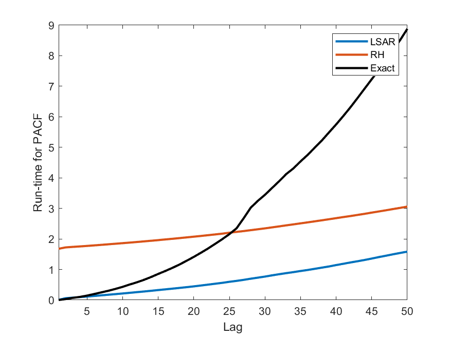
(a) $\mathtt{AR(5)}$

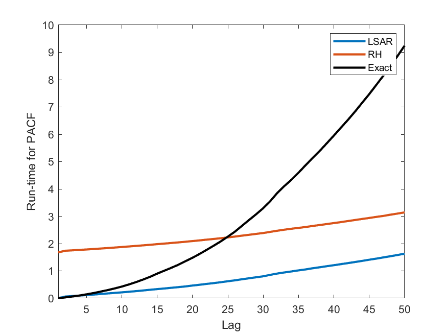
(b) $\mathtt{AR(10)}$

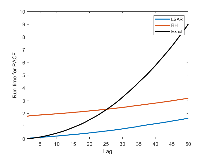
(c) $\mathtt{AR(20)}$

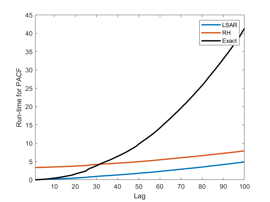
(d) $\mathtt{AR(50)}$

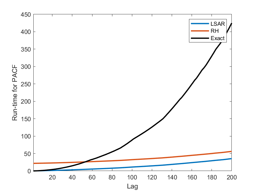
(e) $\mathtt{AR(100)}$

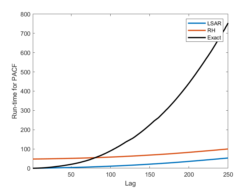
(f) $\mathtt{AR(150)}$

Figure 1: Figures (a) to (f) corresponding to the labeled AR$(p)$ models, show the comparison between the computation time (in seconds) to generate the PACF for the LSAR algorithm (in blue), the Repeated Halving algorithm (in red) and the exact computation of PACF (in black).

(a) $\mathtt{AR(5)}$

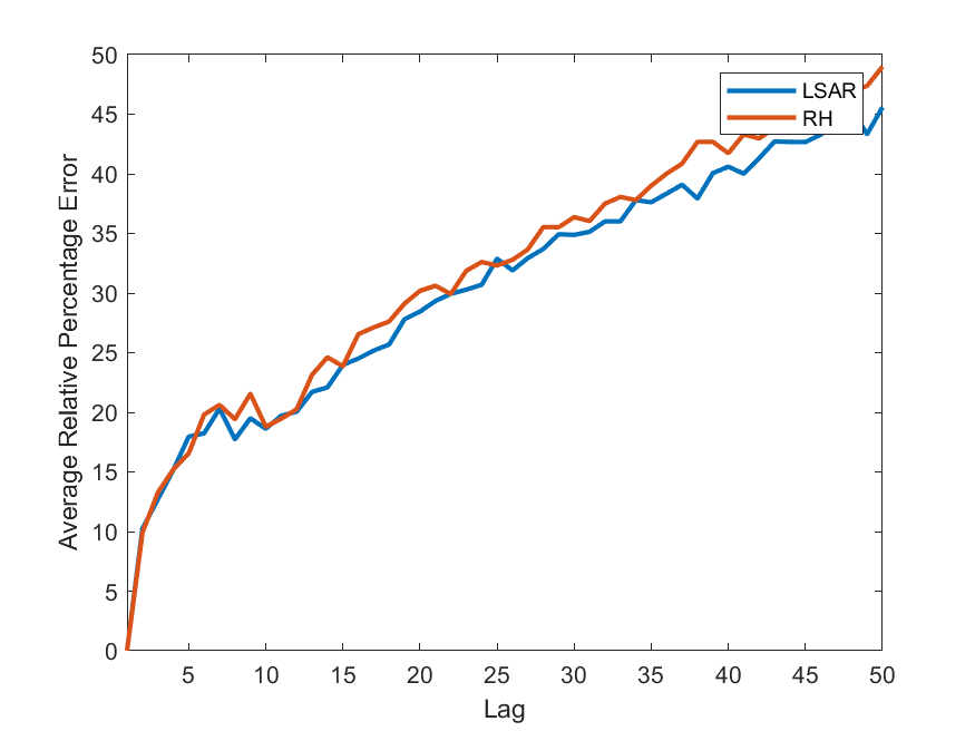
(b) $\mathtt{AR(10)}$

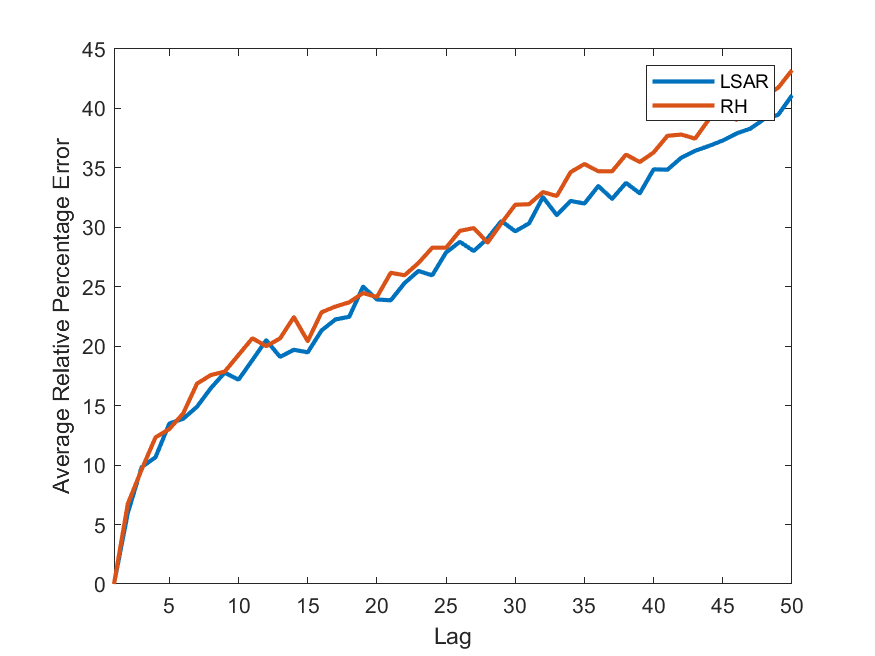
(c) $\mathtt{AR(20)}$

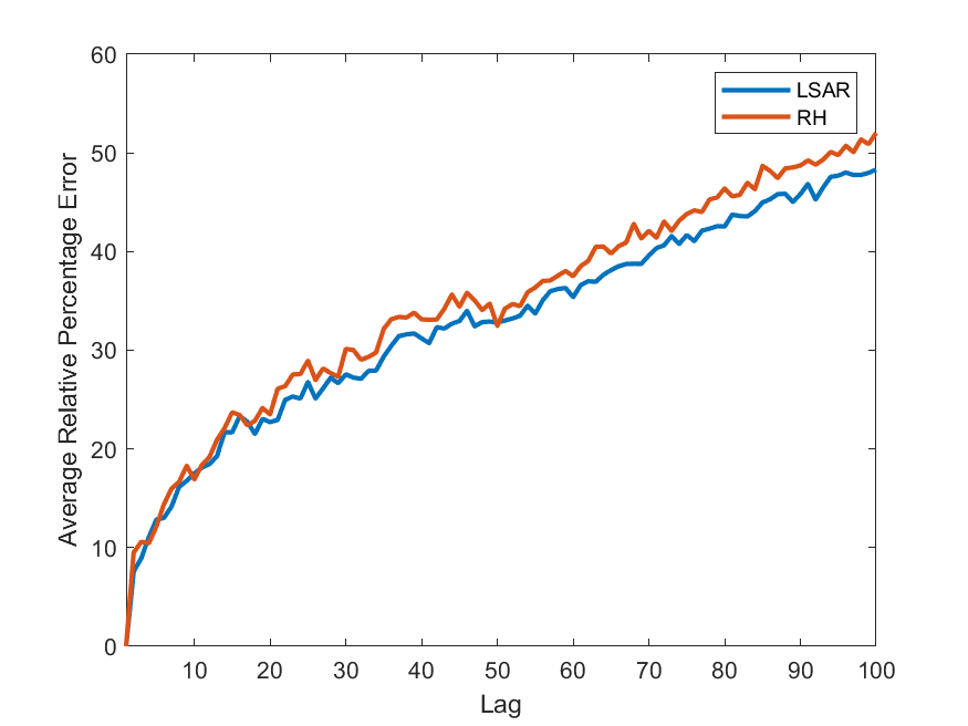
(d) $\mathtt{AR(50)}$

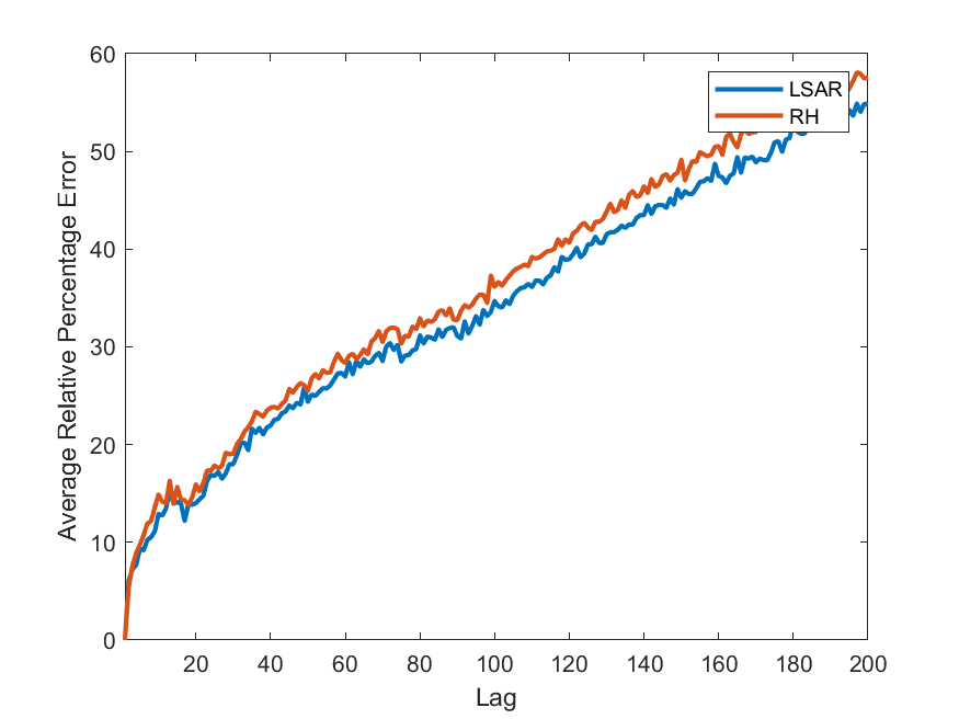
(e) $\mathtt{AR(100)}$

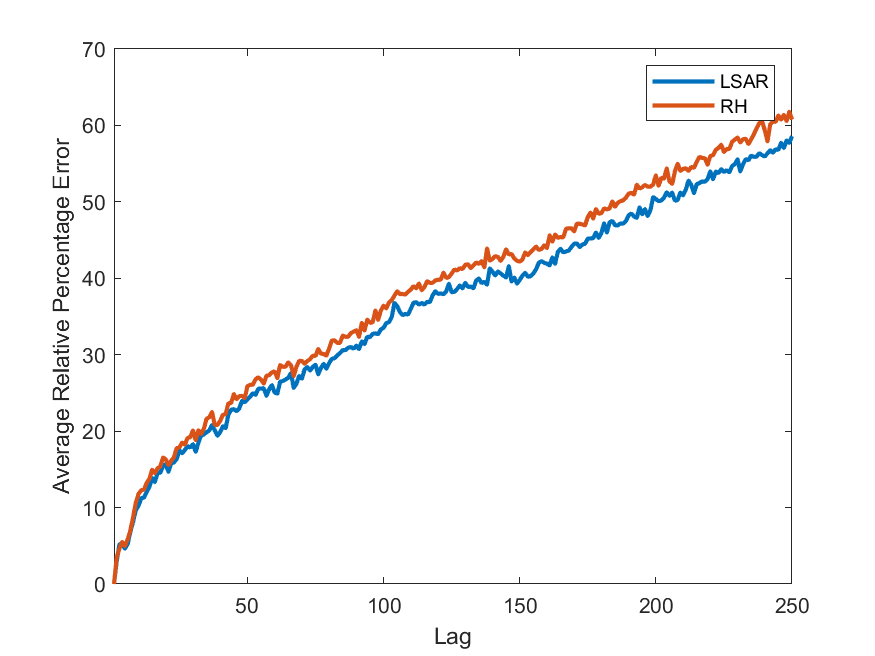
(f) $\mathtt{AR(150)}$

Figure 2: Figures (a) to (f) corresponding to the labeled AR$(p)$ models, show the percentage relative error in $\bm{\phi}$ given by 14 at each lag, for values of $\bm{\phi}$ determined by the LSAR algorithm (in blue) and the Repeated Halving algorithm (in red). The average error was computed after running the algorithms 50 times.

4.1.2 Estimation Quality

To look at the estimation quality of each algorithm we compare how well they find the maximum likelihood estimates $\bm{\phi}$ of the models’ parameters at each lag.

When fitting an AR$(p)$ model, we find the maximum likelihood estimates of $\bm{\phi}$ at each lag. Each algorithm derives estimates of $\bm{\widehat{\phi}}^{s}_{p,h}$ based on the compressed data matrices. We can also calculate the estimate of $\bm{\widehat{\phi}}_{p,h}$ exactly using the full data matrix. To examine the quality of the algorithms, we wish to look at the relative difference between each algorithm’s maximum likelihood estimates of the parameters (based on the compressed data matrices) and the estimate based on the full data matrix (the exact algorithm). For this purpose we define the relative percentage error as

$$\frac{\|\bm{\widehat{\phi}}^{s}_{p,h}-\bm{\widehat{\phi}}_{p,h}\|}{\|\bm{\widehat{\phi}}_{p,h}\|}\times 100.$$ (14)

Figure 2 compares the average relative percentage error, at each lag, between the LSAR algorithm and the RH algorithm for each AR$(p)$ model. Once again we have used 2 million synthetically generated data points, and the hyper-parameter $c$ (the number of sampled rows) was $2,000$ ($0.1\%$ of the data). To smooth out the error curves, the algorithms were repeated 50 times and the mean of error at each lag was computed after excluding 5% of the data values at each end of the data set. This was done to remove outliers.

As we can see in Figure 2, despite the LSAR and RH algorithms taking very different approaches to obtaining leverage scores for sampling the data, the difference in the resultant estimated parameters in negligible.

4.1.3 PACF Plots

In this section, we compare the PACF plots for each AR$(p)$ synthetic data set. The PACF plot is of primary importance in the time series analysis process. We discussed in Section 3 that in order to estimate the order $p$ of a time series, we can use the PACF (8). The PACF plot displays the PACF at each lag as a bar graph. The order $p$ is estimated by choosing the largest lag in the PACF plot where the corresponding PACF is outside the 95% zero confidence boundary.

Figures 3, LABEL: and 4 display the PACF plots generated by each algorithm, for all synthetic data sets. We estimate the PACF for each lag up to $\bar{p}$, first using the full data matrix, then twice more using the PACF obtained by each of the compressed data matrices of the LSAR and RH algorithms respectively. For each AR$(p)$ model we use the same data sets from Section 4.1.1, with $n=2,000,000$ and number of sampled rows $c=2,000$. The dashed red error lines indicate the 95% zero confidence boundary.

In Figures 3, LABEL: and 4 we are able to obtain a correct estimate of the order $p$ for the generated synthetic data from each of the exact, LSAR and RH algorithms. All PACF plots generated by the compressed data matrices appear to be quite similar to the corresponding exact PACF plots. This is by sampling only 0.1% of the rows of the data matrix.

There is clearly some error at each lag of the compressed algorithms. This is particularly evident at lags greater than the order of the model, which should be closer to zero. However, while we should be aware of this error, it must be noted that it does not affect the estimation of the order in the synthetic data examples that we present. Furthermore, we are able to obtain these reasonable approximations of the PACF in a significantly reduced time when compared to the exact alternative.

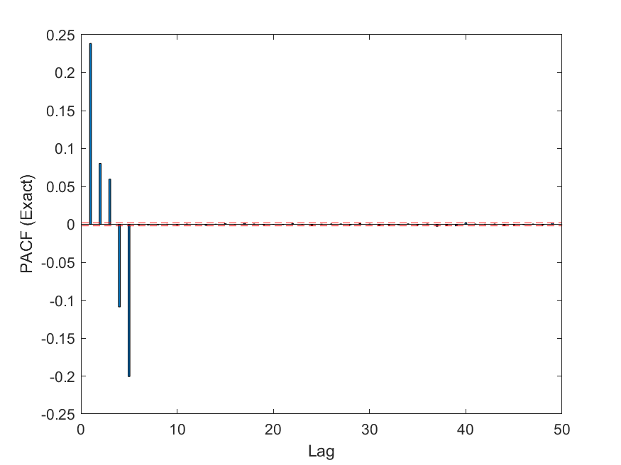
(a) $\mathtt{AR(5)}$

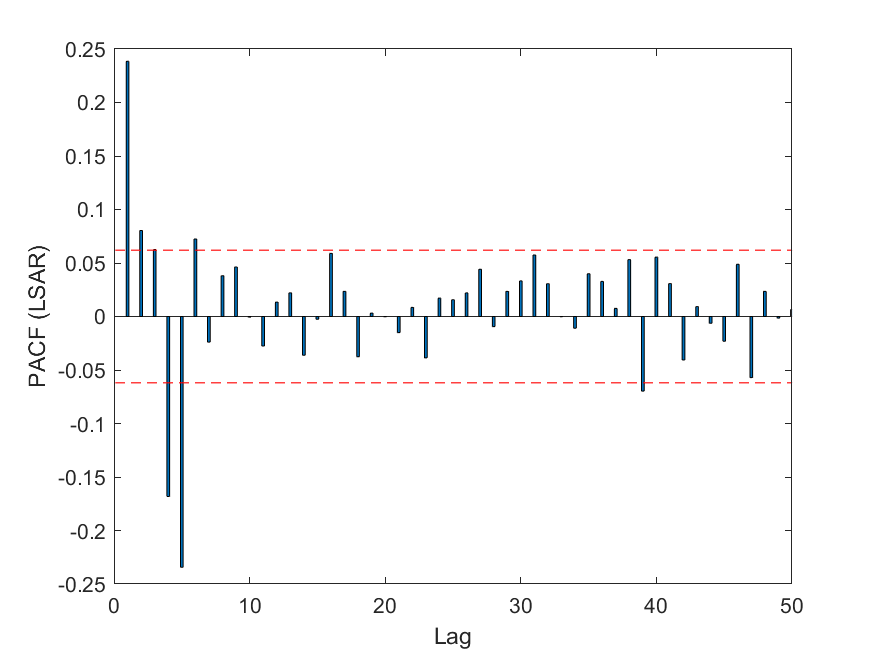
(b) $\mathtt{AR(5)}$

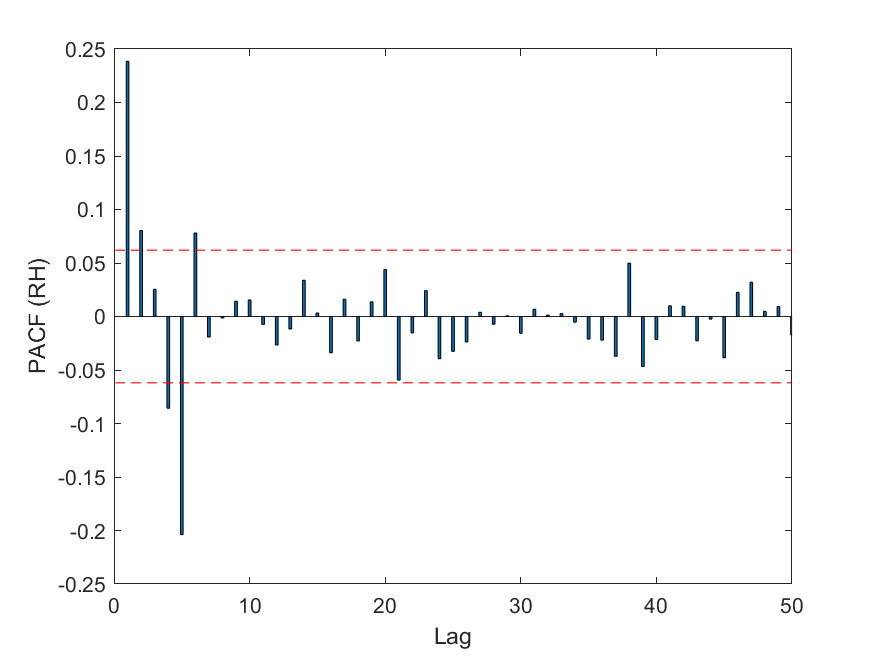
(c) $\mathtt{AR(5)}$

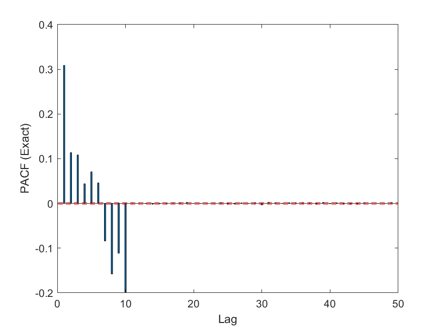
(d) $\mathtt{AR(10)}$

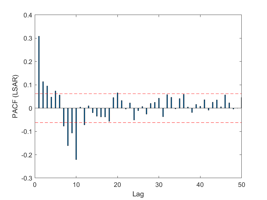
(e) $\mathtt{AR(10)}$

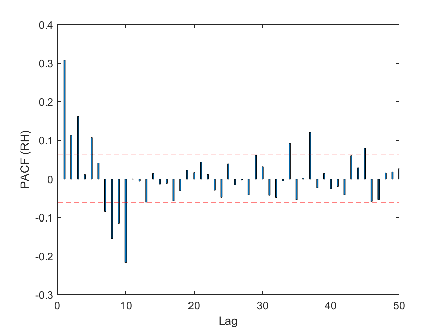
(f) $\mathtt{AR(10)}$

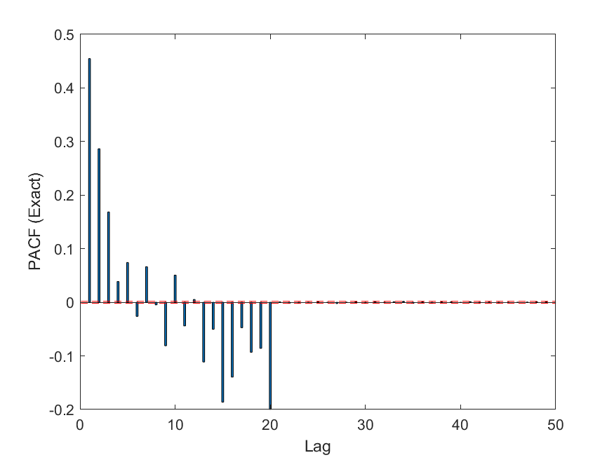
(g) $\mathtt{AR(20)}$

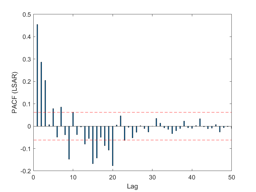
(h) $\mathtt{AR(20)}$

(i) $\mathtt{AR(20)}$

Figure 3: Figures (a) to (c), (d) to (f) and (g) to (i) correspond to randomly generated data from AR$(5)$, AR$(10)$ and AR$(20)$ models respectively. For each model we show the PACF plot computed exactly by the LSAR algorithm and by the RH Algorithm. These are displayed from left to right, respectively. Excluding some noise, we are able use the PACF plots to correctly identify the order $p$ of the data sets, even though the sampled algorithms use only $0.1\%$ of the data.

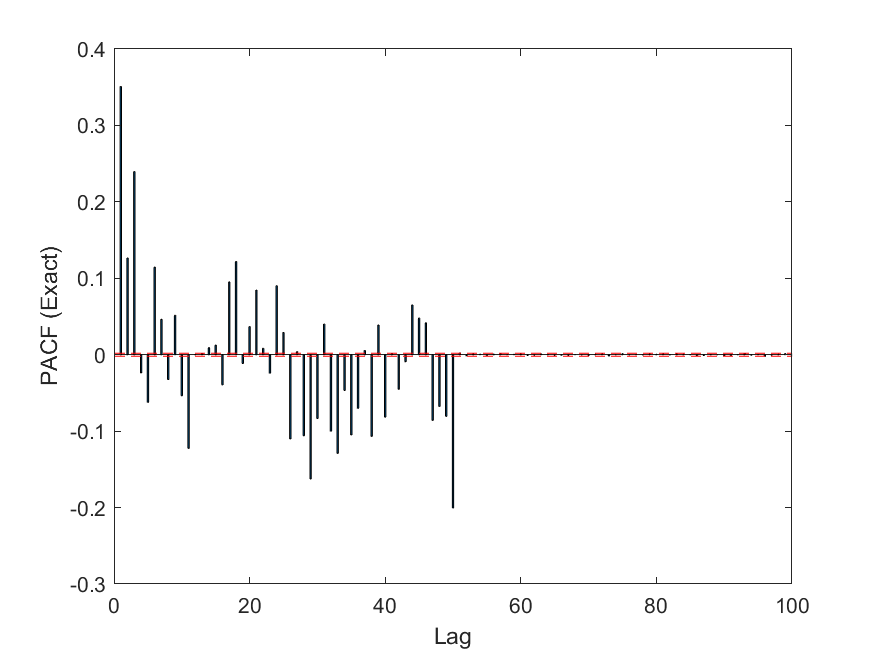
(a) $\mathtt{AR(50)}$

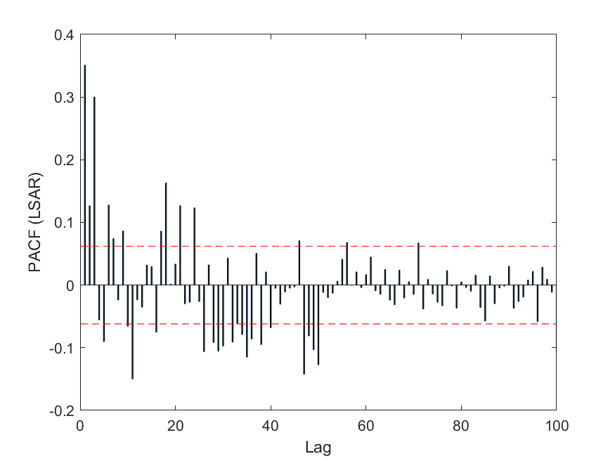
(b) $\mathtt{AR(50)}$

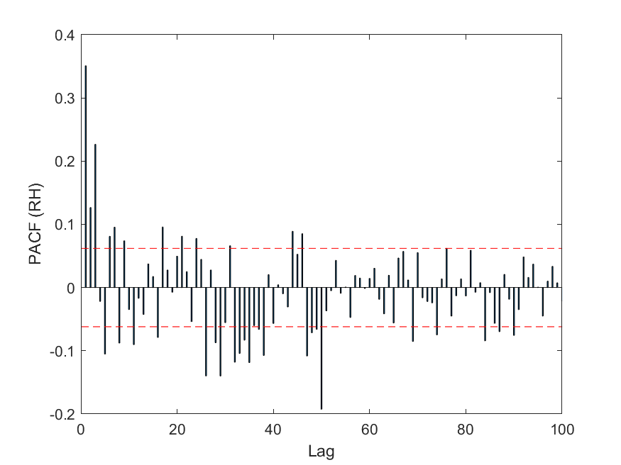
(c) $\mathtt{AR(50)}$

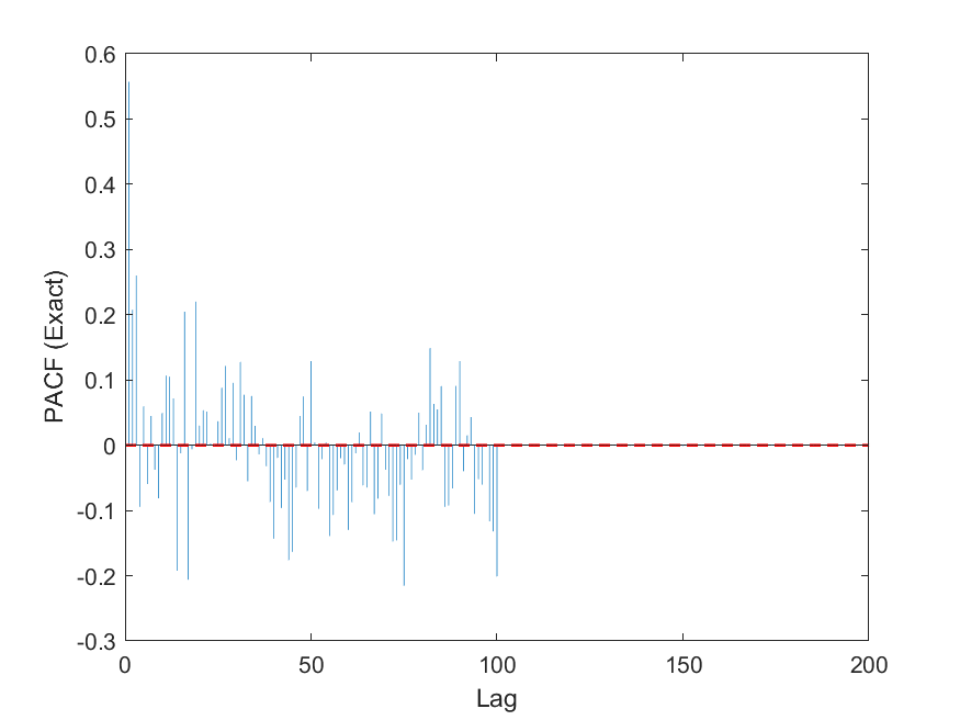
(d) $\mathtt{AR(100)}$

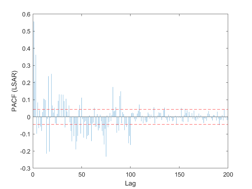
(e) $\mathtt{AR(100)}$

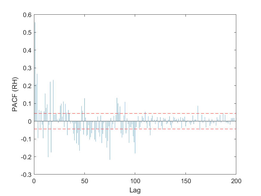
(f) $\mathtt{AR(100)}$

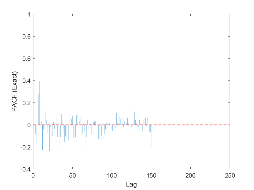
(g) $\mathtt{AR(150)}$

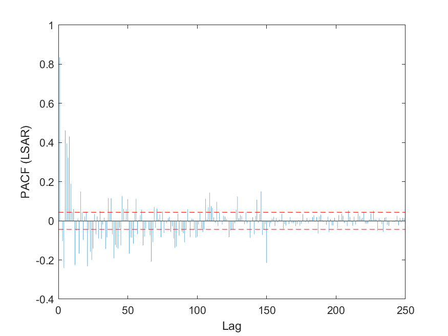
(h) $\mathtt{AR(150)}$

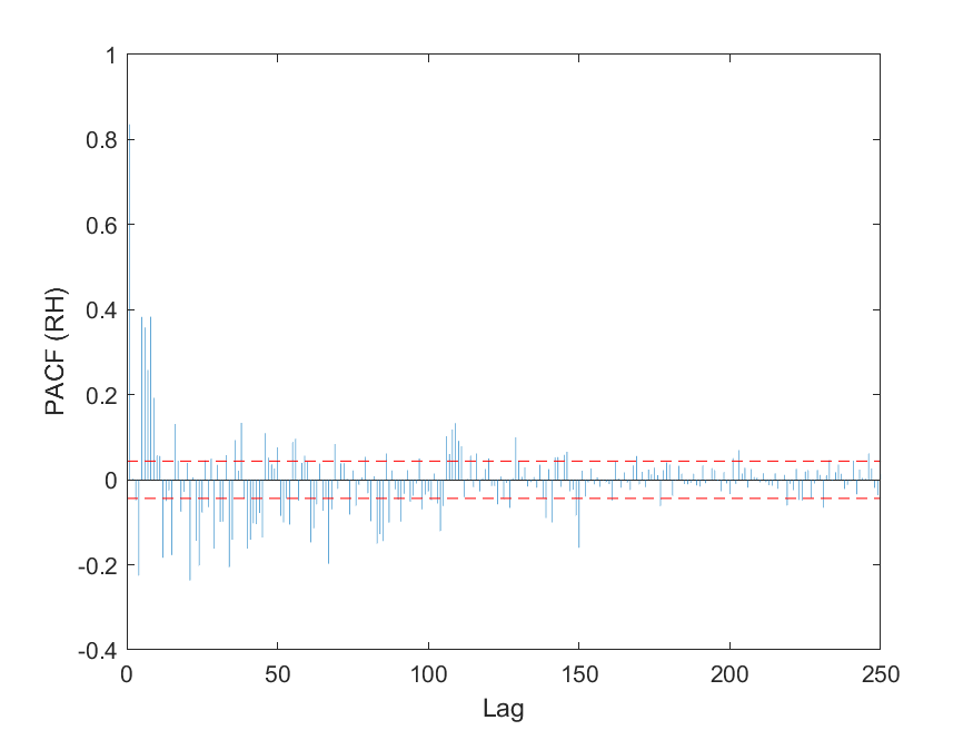
(i) $\mathtt{AR(150)}$

Figure 4: Figures (a) to (c), (d) to (f) and (g) to (i) correspond to randomly generated data from AR$(50)$, AR$(100)$ and AR$(150)$ models respectively. For each model we show the PACF plot computed exactly by the LSAR algorithm and by the RH Algorithm. These are displayed from left to right, respectively. Excluding some noise, we are able to use the PACF plots to correctly identify the order $p$ of the data sets, even though the sampled algorithms use only $0.1\%$ of the data.

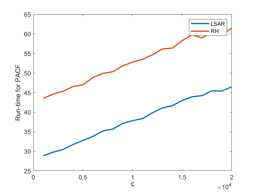
(a) Time

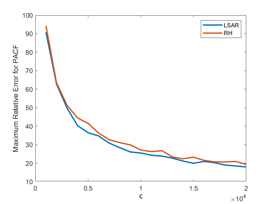
(b) Error

Figure 5: Figure (a) displays the run time of the LSAR algorithm (in blue) and the RH algorithm (in red) when run multiple time over different values of $c$. Figure (b) displays the maximum point-wise value of relative percentage error for each of the algorithms.

4.1.4 The Effect of Sample Size

We recall that the LSAR and RH algorithms have hyper-parameter $c$, the number of rows sampled from the full data matrix to construct the compressed data matrices used by these algorithms. Choosing different values of $c$ leads to a trade-off between run time and accuracy of the compressed algorithms. For example, if we used a larger value of $c$ we would expect our accuracy to increase (or our error to decrease) at the expense of computation time.

Figure 5 displays the computation time and relative percentage error (given by 14) as $c$ changes for a synthetically generated AR$(100)$ data set with $n=2,000,000$. Maximum point-wise time and error over the lags was taken for each instance of the algorithm running for $c=\{1000,2000,\dots,20,000\}$ and is displayed in Figures 5(a), LABEL: and 5(b) respectively.

Figure 5 confirms the discussed trade-off between time and error. Computation time appears to increase linearly as a function of $c$, while the error decreases.

4.2 Synthetic Data with Outliers

This section follows a similar pattern to Section 4.1, except this time with the addition of outliers in the data. Once again, two million realisations from six AR$(p)$ time series models were randomly generated for $p=5,10,20,50,100,150$ with coefficients corresponding to a stationary time series model for each order obtained randomly. Synthetic data was generated with constant 0 and variance 1. One thousand data points were randomly selected and replaced with the sum of the data point, a randomly generated number from a uniform distribution over $[-3,3]$, and a normally distributed variable with a mean of 0 and variance of 100.

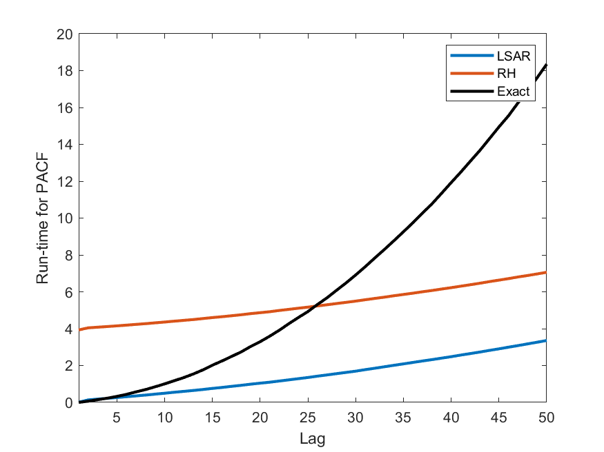
(a) $\mathtt{AR(5)}$

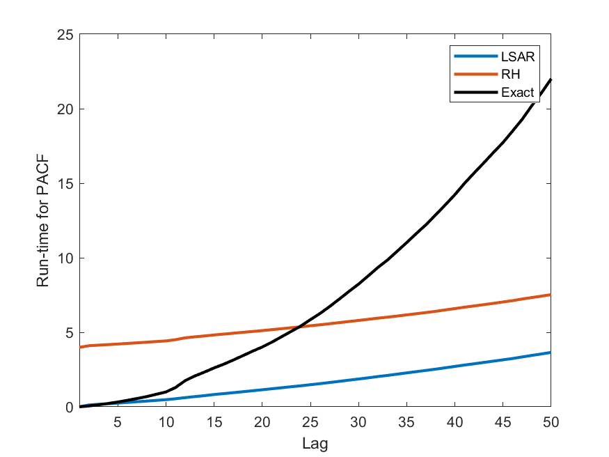
(b) $\mathtt{AR(10)}$

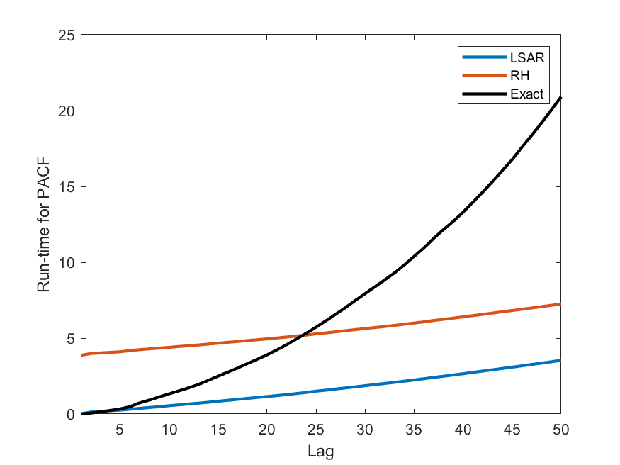
(c) $\mathtt{AR(20)}$

(d) $\mathtt{AR(50)}$

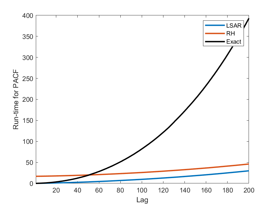
(e) $\mathtt{AR(100)}$

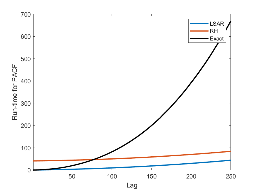
(f) $\mathtt{AR(150)}$

Figure 6: Figures (a) to (f) corresponding to the labeled AR$(p)$ models, compare the computation time (in seconds) to generate the PACF for the LSAR algorithm (in blue), the Repeated Halving algorithm (in red) and the exact computation of PACF (in black).

4.2.1 Computational Time of the PACF

Similarly to Section 4.1.1, Figure 6 compares the run time to compute the PACF by the LSAR algorithm, the RH algorithm, and the exact calculation, for each AR$(p)$ model. Time is plotted cumulatively over each lag.

The computation times of the algorithms, including the exact computations, are unaffected by the presence of outliers. We note that computation times are approximately the same as those in Section 4.1.1 because we are performing calculations on matrices of the same size. The RH and LSAR algorithms appear to have similar computation times, separated by a constant, which is due to the RH algorithm computing leverage scores prior to the algorithm’s iteration over the lag. In particular, the difference in computation time is exemplified by Figure 6(f), which presents a 700-second difference between the exact method and the two compressed methods.

4.2.2 Estimation Quality

We examine the estimation quality of each algorithm, as in Section 4.1.2, by comparing how well they find the maximum likelihood estimates $\bm{\phi}$ of the models’ parameters at each lag. This time, the models include outliers.

Figure 7 compares the relative percentage error according to 14, at each lag, between the LSAR algorithm and the RH algorithm for each AR$(p)$ model. We have used 2 million synthetically generated data points with 1000 replaced by outliers as discussed in Section 4.2. The number of sampled rows $c$ was $2,000$ ($0.1\%$ of the data). To smooth out the error curves, the algorithms were repeated 50 times and the mean of error at each lag was computed after excluding 5% of the data values at each end of the data set. This was done to remove outliers. Thus each graph pertains to the average relative percentage error.

In Figure 7, we can again observe that despite LSAR and RH taking very different approaches to obtaining leverage scores for sampling the data, the difference between the resultant estimated parameters is negligible. There also appears to be negligible difference between the errors of the algorithms for the data sets with and without outliers. This would suggest that the presence of outliers has very little effect on the estimated parameters for each algorithm.

4.2.3 PACF Plots

Figures 8, LABEL: and 9 display the PACF plots generated by each algorithm, for all synthetic data sets with included outliers. We estimate the PACF using the full data matrix and each of the compressed data matrices as we did in Section 4.1.3. For each AR$(p)$ model we use the same data sets from Section 4.2.1, with $n=2,000,000$ and number of sampled rows $c=2,000$.

We are able use the PACF plots of the compressed algorithms to correctly identify the order $p$ of the data sets, notwithstanding some error. The plots were obtained using only $0.1\%$ of the data. As we saw in Section 4.2.1, the algorithms took significantly less time than the exact method, and were unaffected by outliers.

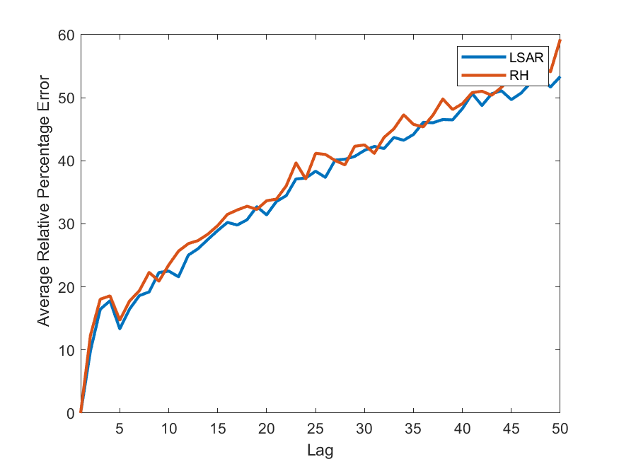
(a) $\mathtt{AR(5)}$

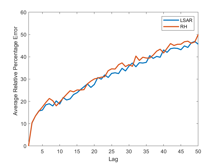
(b) $\mathtt{AR(10)}$

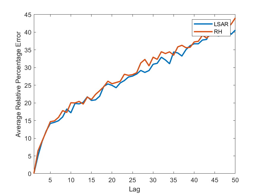
(c) $\mathtt{AR(20)}$

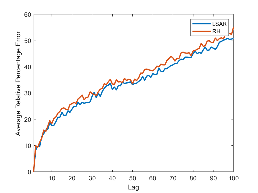
(d) $\mathtt{AR(50)}$

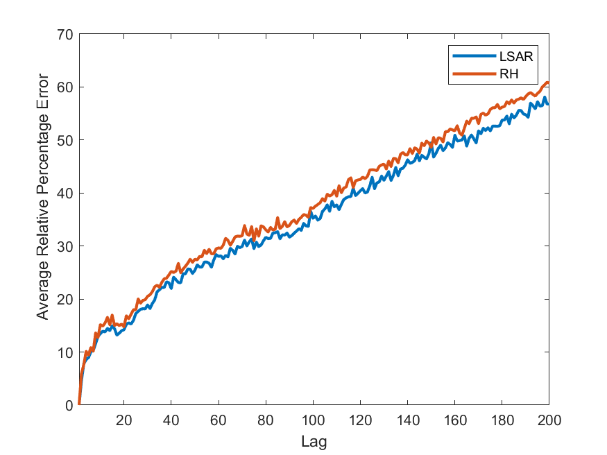
(e) $\mathtt{AR(100)}$

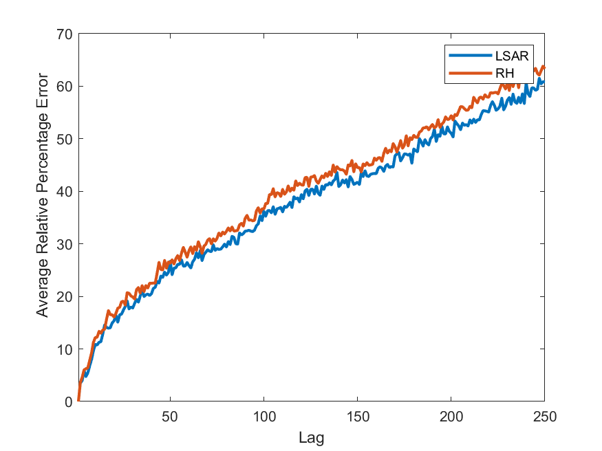
(f) $\mathtt{AR(150)}$

Figure 7: Figures (a) to (f) corresponding to the labeled AR$(p)$ models show the percentage relative error in $\bm{\phi}$ given by 14 at each lag, for values of $\bm{\phi}$ determined by the LSAR algorithm (in blue) and the Repeated Halving algorithm (in red). The average error was computed after running the algorithms 50 times.

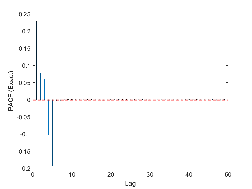
(a) $\mathtt{AR(5)}$

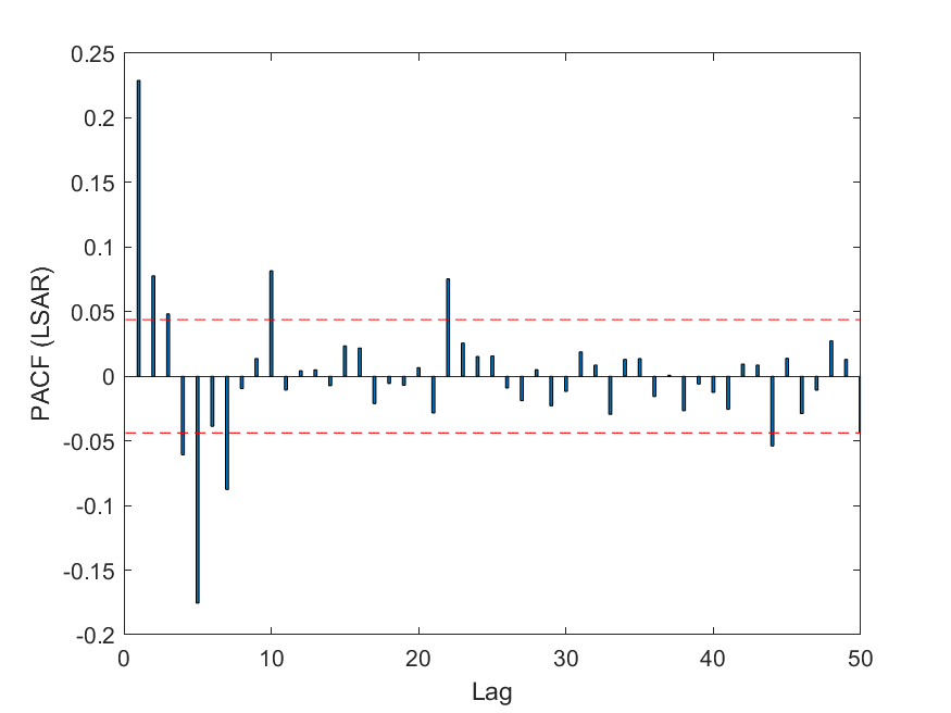
(b) $\mathtt{AR(5)}$

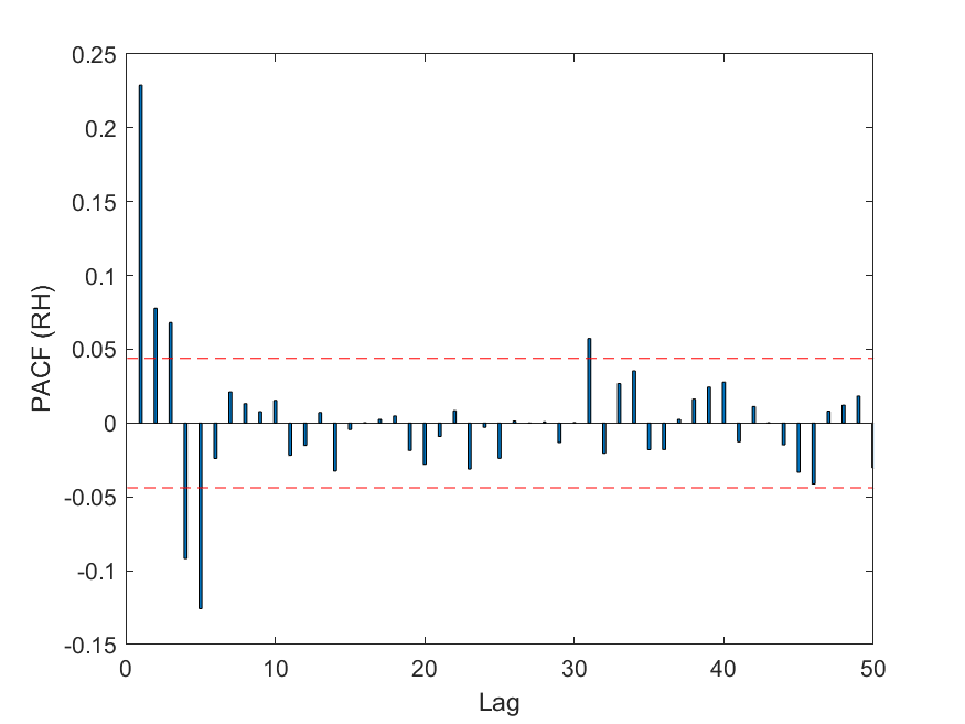
(c) $\mathtt{AR(5)}$

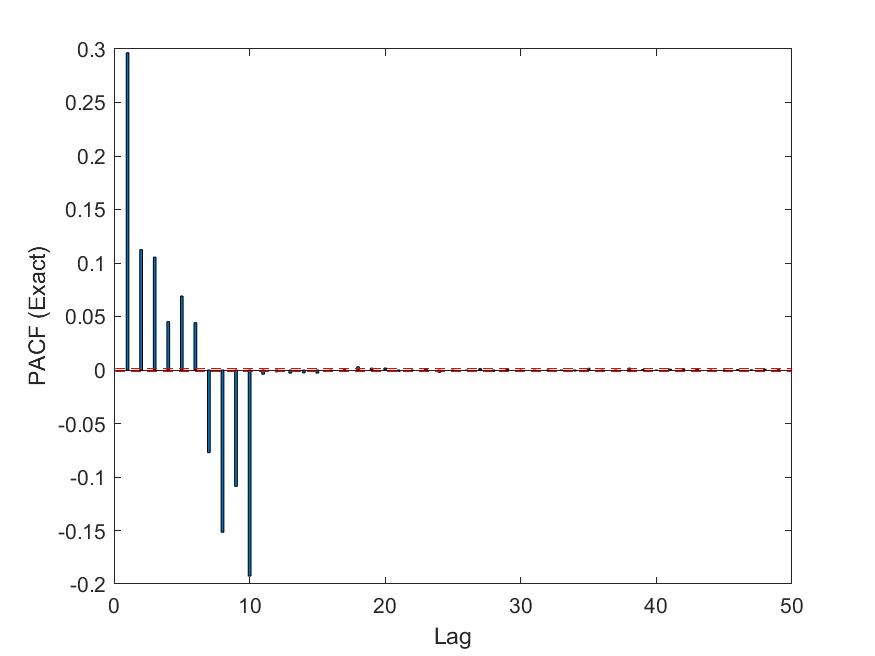
(d) $\mathtt{AR(10)}$

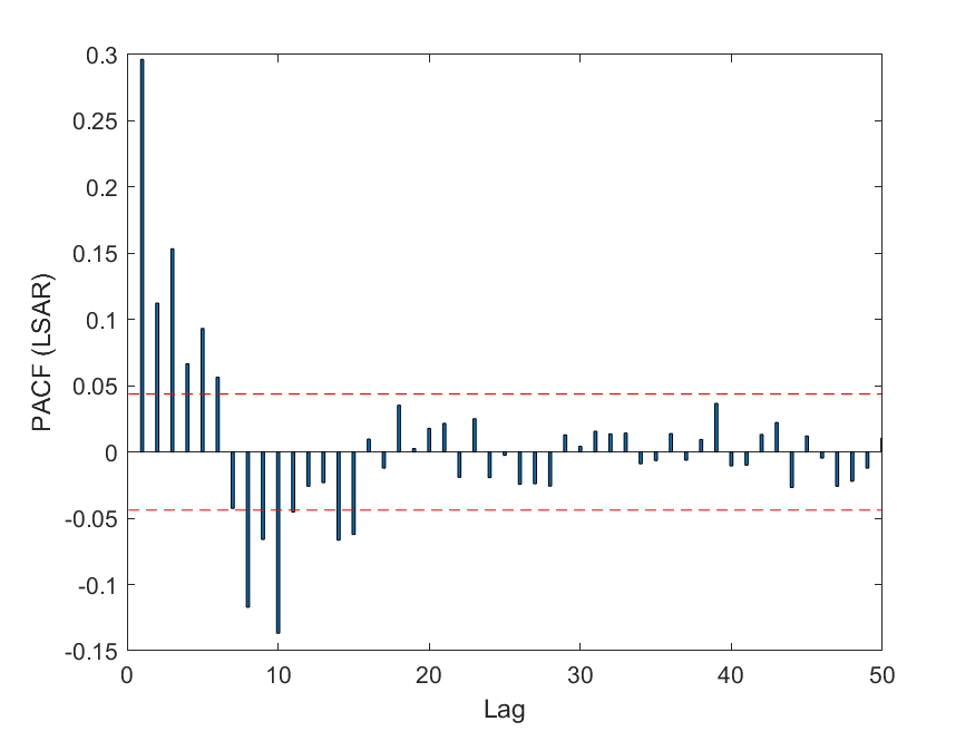
(e) $\mathtt{AR(10)}$

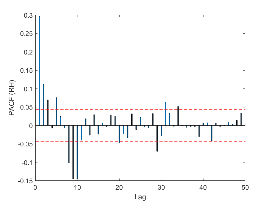
(f) $\mathtt{AR(10)}$

(g) $\mathtt{AR(20)}$

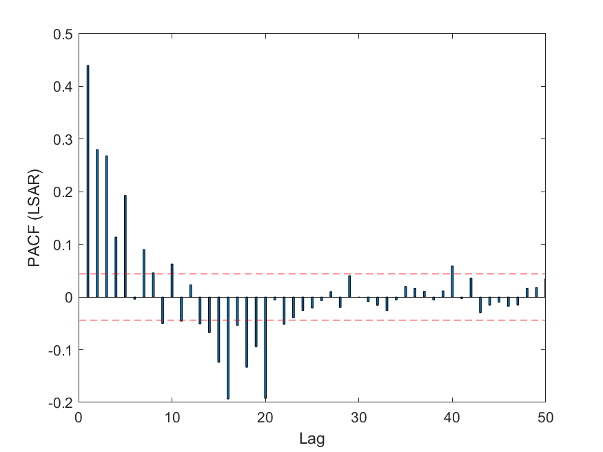
(h) $\mathtt{AR(20)}$

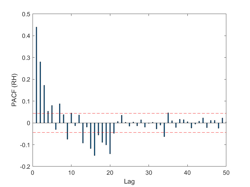
(i) $\mathtt{AR(20)}$

Figure 8: Figures (a) to (c), (d) to (f) and (g) to (i) correspond to randomly generated data from AR$(5)$, AR$(10)$ and AR$(20)$ models (with outliers) respectively. For each model we show the PACF plot computed exactly, by the LSAR algorithm and by the RH Algorithm. These are displayed from left to right, respectively.

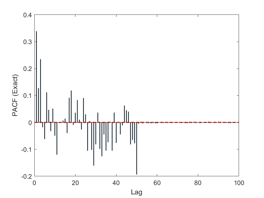
(a) $\mathtt{AR(50)}$

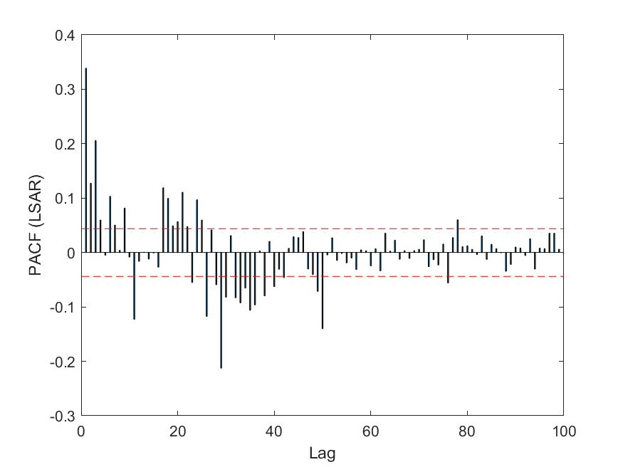
(b) $\mathtt{AR(50)}$

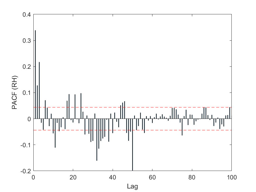
(c) $\mathtt{AR(50)}$

(d) $\mathtt{AR(100)}$

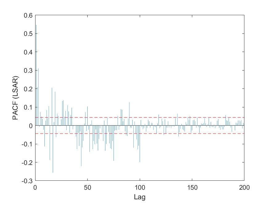
(e) $\mathtt{AR(100)}$

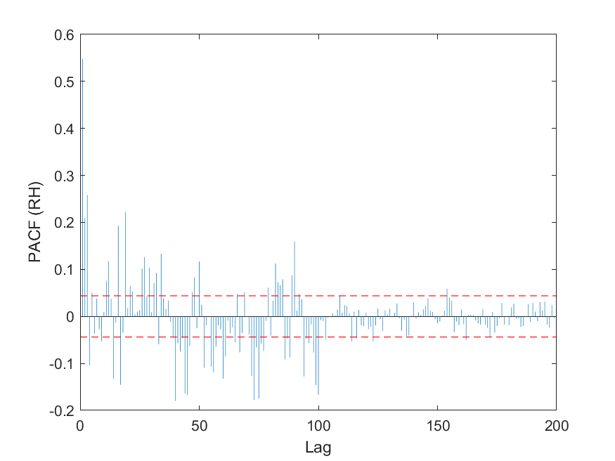
(f) $\mathtt{AR(100)}$

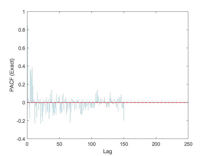
(g) $\mathtt{AR(150)}$

(h) $\mathtt{AR(150)}$

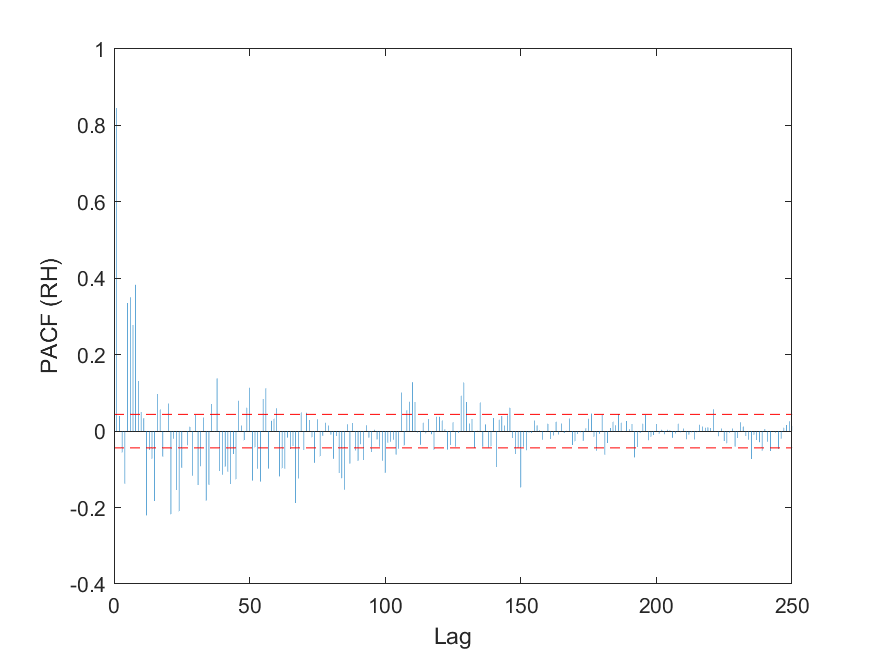
(i) $\mathtt{AR(150)}$

Figure 9: Figures (a) to (c), (d) to (f) and (g) to (i) correspond to randomly generated data from AR$(50)$, AR$(100)$ and AR$(150)$ models (with outliers) respectively. For each model we show the PACF plot computed exactly, by the LSAR algorithm and by the RH Algorithm. These are displayed from left to right, respectively. We are able use the PACF plots to correctly identify the order $p$ of the data sets.

4.3 Real-world Data

We now test the quality and run time of the algorithms on some real-world data. We turn to data collected by Huerta et al. [23] studying the accuracy of electronic nose measurements. An electronic nose is an array of metal-oxide sensors capable of detecting chemicals in the air as a way of mimicking how a human or animal nose works. In this study the nose was constructed from eight different metal-oxide sensors, as well as humidity and temperature sensors. Measurements from each of these sensors were taken simultaneously at a rate of one observation per second for a period of almost two years in one of the author’s home. Huerta et al. were able to use a statistical model utilising measurements from the nose to discriminate between different gasses with an R-squared close to 1.

The data was obtained from the UCI machine learning repository [22]. We look specifically at measurements of the eighth metal-oxide sensor (column R8 in the data set). The data set has $n=919,438$ observations, and we must transform the data by taking the logarithm and difference in one lag to obtain a stationary data set.

As we have for our synthetic data sets, we compare the run time, error and PACF plots for each of the LSAR algorithm, the RH algorithm and the exact calculation. The algorithms are run with $\bar{p}=100$, and the number of rows sampled for each of the compressed algorithms was $s=0.01n=9194$.

Figure 10 displays the run time and the error of the estimated maximum likelihood error for the LSAR algorithm, the RH algorithm, and the exact calculation on the gas sensor data.

(a) computation time

(b) relative percentage error

Figure 10: Figure (a) corresponding to the gas sensor data, shows the comparison between the computation time (in seconds) to generate the PACF for the LSAR algorithm (in blue), the RH algorithm (in red) and the exact computation of PACF (in black). Figure (b) shows the average relative percentage error over 50 runs of the algorithms, for each lag $h$

To smooth out the error curves in Figure 10(b), the algorithms were repeated 50 times and the mean of error at each lag was computed after excluding 5% of the data values at each end of the data set. This was done to remove outliers.

The run times of all three algorithms, shown in Figure 10(a), tell a similar story to that of Sections 4.1.1 and 4.2.1. However, Figure 10(b) displays a different pattern of error from what we have previously seen. Instead of steadily rising and being of similar magnitude to the LSAR algorithm, the RH algorithm jumps to 10% error in the first lag before steadily rising. On the other hand, error in the parameters of LSAR algorithm is robust and consistent with the numerical results that we have presented in the synthetically generated data sections.

This pattern of errors in the estimated parameters is reflected in the PACF plots produced by each of the algorithms (displayed in Figure 11). From Figure 11(b), the PACF plot generated by the LSAR algorithm excellently replicates the PACF plot of the exact algorithm, and it would seem that AR$(18)$ would be a good fit for this data set according to both the exact and LSAR algorithms. Figure 11(c) on the other hand reaches the 95% zero confidence bounds much earlier, suggesting that it would incorrectly estimate the order to fit to the data set.

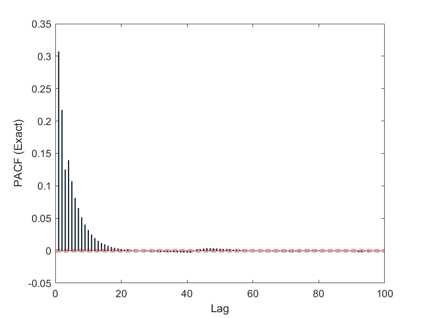
(a) Exact

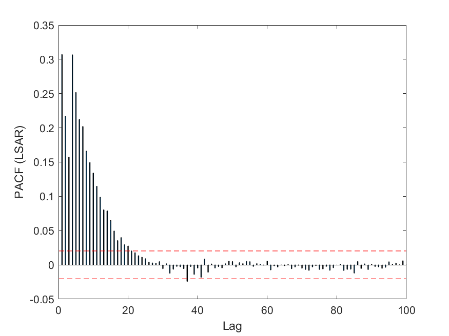
(b) LSAR

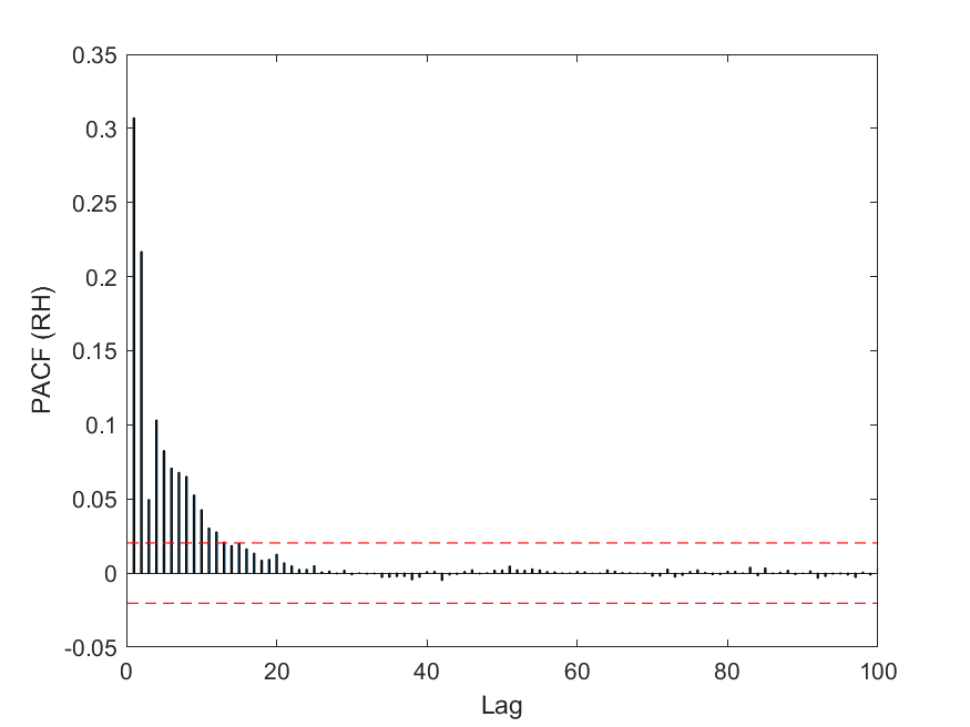
(c) RH

Figure 11: Figures (a), (b) and (c) display the exact PACF plot, the PACF plot computed by the LSAR algorithm and the PACF plot computed using the RH algorithm respectively. Each plot corresponds to the gas sensor data of [23].

5 Conclusion

We have examined the application of RandNLA to large time-series data. To do this we compared the LSAR and RH algorithms over a range of problem sizes with synthetic data and also some real data. As expected, because the algorithms solve subproblems with significantly smaller data matrices, the time to solve OLS problems associated with fitting an AR model was considerably reduced. In addition, the errors of the estimated model parameters were small and similar for both algorithms for each of the synthetic data sets. When applied to real time-series data, the two algorithms again had comparable run time; however, the LSAR algorithm elicited less error when estimating parameters.

The low error in the estimated parameters speaks to the utility of the algorithms for fitting an AR model. The AR fitting process involves two steps: estimating the order (from the PACF), then obtaining parameters of the model with best fitting order. Utility here refers to how the PACF plots generated by the algorithms provide it with accurate and usable information. For all synthetic models the PACF plot generated could be used to identify the order of the model, give or take some noise.

Overall, this paper displays the effectiveness of RandNLA in a time series context. We also see how the LSAR algorithm could provide a framework with which to adapt another Toeplitz least squares solver, the RH algorithm, to a time series context. Future work could look at adapting other Toeplitz least squares solvers such as those in [28, 26] to a time series context and also compare the accuracy of these solvers when the problem involves ill-conditioned matrices.

References

- [1] M. Abolghasemi, J. Hurley, A. Eshragh, and B. Fahimnia. Demand forecasting in the presence of systematic events: Cases in capturing sales promotions. International Journal of Production Economics, 230:107892, 2020.
- [2] K. Avrachenkov, A. Eshragh, and J. Filar. On transition matrices of Markov chains corresponding to hamiltonian cycles. Annals of Operations Research, 243(1):19–35, 2016.
- [3] N. G. Bean, R. Elliott, A. Eshragh, and J. V. Ross. On binomial observation of continuous-time Markovian population models. Journal of Applied Probability, 52:457–472, 2015.
- [4] N. G. Bean, A. Eshragh, and J. V. Ross. Communications in statistics: Theory and methods. Annals of Operations Research, 45(24):7161–7183, 2016.
- [5] K. L. Clarkson and D. P. Woodruff. Low-rank approximation and regression in input sparsity time. Journal of the ACM (JACM), 63(6):54, 2017.
- [6] M. B. Cohen, Y. T. Lee, C. Musco, R. Peng, and A. Sidford. Uniform sampling for matrix approximation. In Proceedings of the 2015 Conference on Innovations in Theoretical Computer Science, pages 181–190, 2015.
- [7] P. Drineas, M. Magdon-Ismail, M. W. Mahoney, and D. P. Woodruff. Fast approximation of matrix coherence and statistical leverage. Journal of Machine Learning Research, 13(Dec):3475–3506, 2012.
- [8] P. Drineas and M. W. Mahoney. RandNLA: randomized numerical linear algebra. Communications of the ACM, 59(6):80–90, 2016.
- [9] P. Drineas and M. W. Mahoney. Lectures on randomized numerical linear algebra. CoRR, abs/1712.08880, 2017.
- [10] A. Eshragh. Fisher information, stochastic processes and generating functions. In Proceedings of the 21st International Congress on Modeling and Simulation, 2015.
- [11] A. Eshragh, S. Alizamir, P. Howley, and E. Stojanovski. Modeling the dynamics of the COVID-19 population in Australia: A probabilistic analysis. PLoS ON, 15:e0240153, 2020.
- [12] A. Eshragh and J. Filar. Hamiltonian cycles, random walks and the geometry of the space of discounted occupational measures. Mathematics of Operations Research, 36(2):258–270, 2011.
- [13] A. Eshragh, J. Filar, and M. Haythorpe. A hybrid simulation-optimization algorithm for the Hamiltonian cycle problem. Annals of Operations Research, 189:103–125, 2011.
- [14] A. Eshragh, J. Filar, and A. Nazari. A projection-adapted Cross Entropy (PACE) method for transmission network planning. Energy Systems, 2(2):189–208, 2011.
- [15] A. Eshragh, B. Ganim, T. Perkins, and K. Bandara. The importance of environmental factors in forecasting Australian power demand. Environmental Modeling & Assessment, 2021.
- [16] A. Eshragh, G. Livingston, T. M. McCann, and L. Yerbury. Rollage: Efficient rolling average algorithm to estimate ARMA models for big time series data. arXiv preprint arXiv:2103.09175, 2021.
- [17] A. Eshragh, F. Roosta, A. Nazari, and M. W. Mahoney. LSAR: Efficient leverage score sampling algorithm for the analysis of big time series data. arXiv preprint arXiv:1911.12321, 2019.
- [18] B. Fahimnia, H. Davarzani, and A. Eshragh. Performance comparison of three meta-heuristic algorithms for planning of a complex supply chain. Computers and Operations Research, 89:241–252, 2018.
- [19] B. Fahimnia, J. Sarkis, A. Choudhary, and A. Eshragh. Tactical supply chain planning under a carbon tax policy scheme: A case study. International Journal of Production Economics, 164:206–215, 2015.
- [20] B. Fahimnia, J. Sarkis, and A. Eshragh. Trade-off model for green supply chain planning: A leanness-versus-greenness analysis. International Journal of Production Economics, 54:173–190, 2015.
- [21] J. D. Hamilton. A new approach to the economic analysis of nonstationary time series and the business cycle. Econometrica, 57(2):357–384, 1989.
- [22] F. Huerta and R. Huerta. Gas sensors for home activity monitoring data set. https://archive.ics.uci.edu/ml/datasets/Gas+sensors+for+home+activity+monitoring, 2016.
- [23] R. A. Huerta, T. S. Mosqueiro, J. Fonollosa, N. F. Rulkov, and I. Rodríguez-Luján. Online humidity and temperature decorrelation of chemical sensors for continuous monitoring. Chemometrics and Intelligent Laboratory Systems, 157(15):169–176, 2016.
- [24] M. W. Mahoney. Randomized algorithms for matrices and data. Foundations and Trends® in Machine Learning, 2011.
- [25] X. Shi and D. P. Woodruff. Sublinear time numerical linear algebra for structured matrices. Proceedings of the AAAI Conference on Artificial Intelligence, 33(01):4918–4925, Jul. 2019.
- [26] M. Van Barel, G. Heinig, and P. Kravanja. A superfast method for solving Toeplitz linear least squares problems. Linear Algebra and its Applications, 366:441–457, June 2003.
- [27] D. P. Woodruff. Sketching as a tool for numerical linear algebra. Foundations and Trends® in Theoretical Computer Science, 2014.
- [28] Y. Xi, J. Xia, S. Cauley, and V. Balakrishnan. Superfast and stable structured solvers for Toeplitz least squares via randomized sampling. SIAM Journal on Matrix Analysis and Applications, 35, 01 2014.
- [29] K. Ye and L. Lim. Every matrix is a product of Toeplitz matrices. Foundations of Computational Mathematics, 16(3):577–598, 2016.