Gravitational particle production of superheavy massive particles in Quintessential Inflation II: $\alpha$-attractors

Abstract

We compute the gravitational production of conformally coupled superheavy particles during the phase transition from the end of inflation to the beginning of kination for $\alpha$-attractors potentials in the context of Quintessential Inflation ($\alpha$-QI), showing that the maximum value of the reheating temperature, independently of the value of the parameter $\alpha$, is near $10^{9}$ GeV. This result, which contradicts the usual belief that the reheating via the production of superheavy massive particles leads to an inefficient reheating temperature, is due to the fact that in our numerical calculations we take into account the contribution of the large wavelength modes to the reheating temperature, which never happens in analytical calculations where only ultraviolet modes are considered.

I Introduction

The so-called gravitational particle production Parker ; gmm ; ford ; Zeldovich of superheavy particles conformally coupled with gravity, which was applied to standard inflation (potentials with a deep well) in kolb ; kolb1 ; Birrell1 ; ema , is one of the mechanisms used to reheat the universe in scenarios containing a period of inflation. This also happens in Quintessential Inflation (QI) to match the inflationary period with the usual hot Big Bang universe guth . However, the gravitational reheating in QI is normally applied to very light fields Spokoiny ; pv ; A and only in few papers, which deal with toy non-smooth models as the Peebles-Vilenkin one, it is applied to massive particles H ; ha ; hap18 ; J ; hashiba ; Hashiba . On the other hand, regarding smooth QI potentials, particle creation has to be analytically studied using the complex WKB approximation hashiba1 , whose effective application is limited to the creation of particles by parabolic potentials kofman .

In the present work we continue with our study of particle production by smooth potentials started in ah , now focusing on a smooth exponential potential coming from $\alpha$-attractors in Quintessential Inflation ($\alpha$-QI) vardayan ; K ; benisty3 . Since the $\alpha$-attractors come from supergravity theories containing particles with only gravitational interactions, the late-time decay of these relics may jeopardize the success of the standard BBN lindley . To solve this problem one has to consider sufficiently low reheating temperature (of the order of $10^{9}$ GeV or less) eln . On the contrary, a lower bound for the reheating temperature comes from the fact that the radiation-dominated era occurs before the Big Bang Nucleosynthesis (BBN) epoch, which takes place in the $1$ MeV regime gkr .

Coming back to the gravitational production of superheavy particles, we will use the well-known Hamiltonian diagonalization method (see gmmbook for a review), based on the computation of the time dependent $\beta$-Bogoliubov coefficient which encodes the polarization effects and also the real particles created during the phase transition. Fortunately, these polarization effects disappear when the universe evolves adiabatically, which happens soon after the beginning of kination, allowing its numerical calculation. Thus, in order to calculate the energy density of the produced particles, one can safely use the square modulus of the $\beta$-Bogoliubov coefficient after the beginning of kination, whose numerical value is, for the relevant modes that contribute to the reheating, of the order of $10^{-9}-10^{-10}$ depending on the superheavy masses which in our simulations are of the order of $10^{15}-10^{17}$ GeV.

Finally, once one has the value of the $\beta$-Bogoliubov coefficients, one can calculate the value of the energy density of the superheavy particles, which must decay into lighter ones before or after the end of the kination phase to form a relativistic plasma. In the former case the reheating temperature is greater than $10^{6}$ GeV and in the second one its maximum value is around $10^{9}$ GeV, which shows that the gravitational production of superheavy particles is a very efficient mechanism to reheat our universe.

Throughout the manuscript we use natural units, i.e., $\hbar=c=k_{B}=1$ and the reduced Planck’s mass is denoted by $M_{pl}\equiv\frac{1}{\sqrt{8\pi G}}\cong 2.44\times 10^{18}$ GeV.

II Particle creation of superheavy particles conformally coupled to gravity

We consider a superheavy quantum field $\chi$ conformally coupled with gravity. In order that the polarization effects due to this quantum field do not affect the dynamics of the scalar field responsible for Quintessential Inflation, the mass of the quantum field, namely $m_{\chi}$, must be greater than the Hubble rate, in fact the condition $H\ll m_{\chi}$ has to be satisfied (see Felder to take a look at the problems associated to quantum light fields). Therefore, since the most accepted idea is that inflation starts at GUT scales, where the temperature is around $10^{16}$ GeV, then using the Stefan-Boltzmann law $\rho=\frac{\pi^{2}}{30}g_{*}T^{4}$, where the effective number of degrees of freedom for the Standard model is $106.75$, for a flat FLRW spacetime at the beginning of inflation one has $H\cong 2\times 10^{13}$ GeV. This is the reason why we will chose $m_{\chi}\sim 10^{15}$ GeV or greater.

To calculate the energy density of the produced particles, we will use the well-known diagonalization method, based on the Bogoliubov coefficients, which in the conformally coupled case must satisfy the first order system of differential equations (see gmmbook for a detailed discussion)

$$\left\{\begin{array}[]{ccc}\alpha_{k}^{\prime}(\tau)&=&\frac{\omega_{k}^{\prime}(\tau)}{2\omega_{k}(\tau)}e^{2i\int^{\tau}\omega_{k}(\bar{\tau})d\bar{\tau}}\beta_{k}(\tau)\\ \beta_{k}^{\prime}(\tau)&=&\frac{\omega_{k}^{\prime}(\tau)}{2\omega_{k}(\tau)}e^{-2i\int^{\tau}\omega_{k}(\bar{\tau})d\bar{\tau}}\alpha_{k}(\tau),\end{array}\right.$$ (3)

where the time dependent frequency is denoted by $\omega_{k}(\tau)=\sqrt{k^{2}+m_{\chi}^{2}a^{2}(\tau)}$ and $\tau$ is the conformal time.

Finally, in terms of the $\beta$-Bogoliubov coefficient, the vacuum energy density of the $\chi$-field is given by ah

$$\rho_{\chi}(\tau)=\frac{1}{2\pi^{2}a^{4}(\tau)}\int_{0}^{\infty}k^{2}\omega_{k}(\tau)|\beta_{k}(\tau)|^{2}dk.$$ (4)

II.1 Gravitational particle creation by $\alpha$-attractors in the context of Quintessential Inflation

In the present work, the potential that we will consider is an exponential $\alpha$-attractor in Quintessential Inflation, plotted in Figure 1 and given by

$$V(\varphi)=\lambda M_{pl}^{4}e^{-n\tanh\left(\frac{\varphi}{\sqrt{6\alpha}M_{pl}}\right)},$$ (5)

where $\lambda$, $\alpha$ and $n$ are dimensionless parameters, whose relation is in order to match with the current observation data the following one (see benisty3 for details):

$$\frac{\lambda}{\alpha}e^{n}\sim 10^{-10}\qquad\mbox{and}\qquad\lambda e^{-n}\sim 10^{-120}.$$ (6)

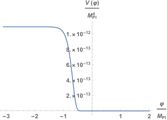
Figure 1: Plot of the Exponential $\alpha$-attractor potential, for $\alpha\sim 10^{-2}$, $n\sim 10^{2}$ and $\lambda\sim 10^{-66}$.

First of all, in order to calculate the energy density of the produced particles one has to integrate numerically the conservation equation for the inflaton field, namely

$$\ddot{\varphi}+3H\dot{\varphi}+V_{\varphi}=0,$$ (7)

where $H=\frac{1}{\sqrt{3}M_{pl}}\sqrt{\frac{\dot{\varphi}^{2}}{2}+V(\varphi)}$, with initial conditions (the value of the scalar field and its first derivative) during inflation. Since the slow-roll regime is an attractor, one only has to take initial conditions in the basin of attraction of the slow-roll solution, for example, $\varphi=\varphi_{*}$ and $\dot{\varphi}=-\frac{V_{\varphi}(\varphi_{*})}{3H_{*}}$, where the “star” denotes that the quantities are evaluated at the horizon crossing.

Once one has obtained the evolution of the scalar field and in particular the evolution of the Hubble rate, one can compute the evolution of the scalar factor, whose value at the horizon crossing we have chosen to be equal to $1$.

From the evolution of the scale factor, we can see on the left-hand side of Figure 2 that a spike appears in the plot of the quantity $\omega_{k}^{\prime}/\omega_{k}^{2}$ during the phase transition from the end of inflation to the beginning of kination, that is, at that moment when the adiabatic evolution is broken and particles are gravitationally produced (see the right-hand side of Figure 2).

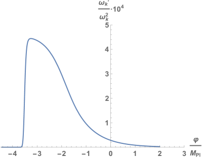
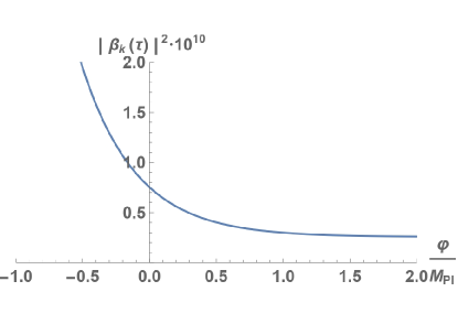
Figure 2: Adiabatic evolution (left) and evolution of the $\beta$-Bogoliubov coefficient (right) for a heavy field with mass $m_{\chi}\sim 10^{16}$ GeV, when $\alpha\sim 10^{-1}$. Here we have used the value $k=a_{kin}H_{kin}$, which is in the range ${k}\lesssim a_{kin}m_{\chi}$, where we have observed that particles are produced.

Then, we have numerically solved equation (3), with initial conditions $\alpha_{k}(\tau_{*})=1$ and $\beta_{k}(\tau_{*})=0$ at the horizon crossing (there were neither particles nor polarization effects at that moment because during the slow-roll regime the derivatives of the Hubble rate are negligible compared with the powers of $H$, i.e., the system is in the adiabatic regime).

For the value $k=a_{kin}H_{kin}$, we obtain in Figure 2 that $|\beta_{k}(\tau)|^{2}$ stabilizes soon to a non-zero value after the beginning of kination, containing only particle production effects. We have numerically done the calculations for masses $m_{\chi}\cong 10^{15}-10^{17}$ GeV and for a large range of values of $\alpha$. We have obtained that the relevant modes that contribute significantly to the particle production are in the range $0\lesssim k\lesssim a_{kin}m_{\chi}$ (see Figure 3), leading to values of $|\beta_{k}|^{2}$ of order $10^{-9}$ for $m_{\chi}\sim 10^{15}$ GeV and values of $|\beta_{k}|^{2}$ of order $10^{-10}$ for $m_{\chi}\sim 10^{16}-10^{17}$ GeV, as one can see in Figure 4.

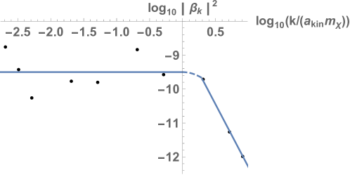
Figure 3: Plot of the logarithm of $|\beta_{k}|^{2}$, as a function of $k$, for a heavy field with mass $m_{\chi}\sim 10^{15}$ GeV and $\alpha=0.1$.

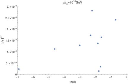
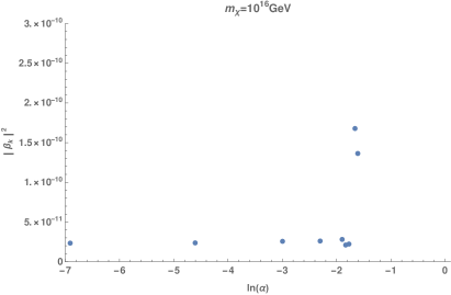
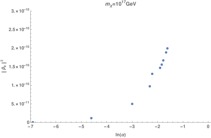
Figure 4: Plot of the square modulus of the $\beta$-Bogoliubov coefficient, as a function of $\alpha$, for a heavy field with masses $m_{\chi}\sim 10^{15}$, $10^{16}$ and $10^{17}$ GeV.

Next, introducing these values of the $\beta$-Bogoliubov coefficient in the energy density (4) and taking into account that the modes that contribute to the energy density satisfy $0\lesssim k\lesssim a_{kin}m_{\chi}$ and lead practically to the same value of the $\beta$-Bogoliubov coefficient, one can safely do the approximation that after the beginning of kination $\omega_{k}(\tau)\cong m_{\chi}a(\tau)$, obtaining

$$\rho_{\chi}(\tau)\cong\frac{m_{\chi}^{4}}{6\pi^{2}}|\beta_{k}|^{2}\left(\frac{a_{kin}}{a(\tau)}\right)^{3}\sim\left\{\begin{array}[]{ccc}10^{-11}m_{\chi}^{4}\left(\frac{a_{kin}}{a(\tau)}\right)^{3}&\mbox{when}&m_{\chi}\sim 10^{15}\mbox{ GeV}\\ &&\\ 10^{-12}m_{\chi}^{4}\left(\frac{a_{kin}}{a(\tau)}\right)^{3}&\mbox{when}&m_{\chi}\sim 10^{16}-10^{17}\mbox{ GeV},\end{array}\right.$$ (11)

for $\tau>\tau_{kin}$.

A final remark is in order: In hashiba ; ema , the authors infer through numerical calculations using toy models that, for the relevant modes, the square of the $\beta$-Bogoliubov coefficient must decay as $e^{-\kappa m_{\chi}/H_{inf}}$, where $H_{inf}$ is the scale of inflation and $\kappa$ a dimensionless factor of order 1. However, throughout all the calculation the mass of the superheavy field is of the same order or less than the scale of inflation. So, in practice, for the relevant models the authors obtain in all numerical simulations $|\beta_{k}|^{2}\geq 10^{-7}$.

In our case we have chosen masses which are many orders greater than the scale of inflation. Effectively, since the power spectrum of scalar perturbations $P_{\zeta}=\frac{H_{*}^{2}}{8\pi^{2}\epsilon_{*}M_{pl}^{2}}\sim 2\times 10^{-9}$ (here, once again, the star denotes that the quantities are evaluated at the horizon crossing) leads to $H_{*}\sim 4\times 10^{-4}\sqrt{\epsilon_{*}}M_{pl}$ -with $\epsilon_{*}=\frac{3\alpha}{16}(1-n_{s})^{2}$ for the case of $\alpha$-attractors, choosing for the spectral index its central value $n_{s}=0.9649$ (see planck )-, one gets the following scale of inflation,

$$H_{*}\sim 1.5\sqrt{\alpha}\times 10^{13}\mbox{ GeV},$$ (12)

which is minimum two orders less than $10^{15}$ GeV.

In summary, there is gravitational production of superheavy particles, with the square of the $\beta$-Bogoliubov, for the relevant modes, of the order of $10^{-9}-10^{-10}$, but for superheavy masses the production is not suppressed by an abnormally small factor as $e^{-\kappa m_{\chi}/H_{inf}}$.

III The reheating process

After the production of the superheavy particles, they have to decay into lighter ones which after the thermalization process form a relativistic plasma that depicts our hot universe. Then, this decay could occur before the end of kination (when the energy density of the inflaton becomes of the same order than the one of the $\chi$-field), or after its end.

III.1 Decay before the end of kination

In this case, the energy density of the background, i.e. the one of the inflaton field, and the one of the relativistic plasma, when the decay is finished, that is when ${\Gamma}\sim H_{dec}=H_{kin}\left(\frac{{a}_{kin}}{a_{dec}}\right)^{3}$, will be

$$\rho_{\varphi,dec}=3{\Gamma}^{2}M_{pl}^{2}\qquad\mbox{and}\qquad\rho_{\chi,dec}=\rho_{\chi,kin}\left(\frac{{a}_{kin}}{a_{dec}}\right)^{3}\cong\frac{m_{\chi}^{4}}{6\pi^{2}}|\beta_{k}|^{2}\frac{\Gamma}{H_{kin}}.$$ (13)

Imposing that the end of the decay precedes the end of kination, which means $\rho_{\chi,dec}\leq\rho_{\varphi,dec}$, and taking into account that it is after the beginning of the kination, i.e., $\Gamma\leq H_{kin}\cong 6\times 10^{-7}M_{pl}$, one gets

$$\frac{1}{18\pi^{2}}|\beta_{k}|^{2}\frac{m_{\chi}^{4}}{H_{kin}M_{pl}^{2}}\leq\Gamma\leq H_{kin}.$$ (14)

Finally, the reheating temperature, i.e., the temperature of the universe when the relativistic plasma in thermal equilibrium starts to dominate, which happens when $\rho_{\varphi,reh}\sim\rho_{\chi,reh}$, can be calculated as follows: Since after the decay the evolution of the respective energy densities are given by

$$\rho_{\varphi,reh}=\rho_{\varphi,dec}\left(\frac{a_{dec}}{a_{reh}}\right)^{6}\qquad\mbox{and}\qquad\rho_{\chi,reh}=\rho_{\chi,dec}\left(\frac{a_{dec}}{a_{reh}}\right)^{4},$$ (15)

we will have $\frac{\rho_{\chi,dec}}{\rho_{\varphi,dec}}=\left(\frac{a_{dec}}{a_{reh}}\right)^{2},$ and thus, from the Stefan-Boltzmann law $\rho_{reh}=\frac{\pi^{2}}{30}g_{reh}T_{reh}^{4}$, where $g_{reh}=106.75$ is the effective number of degrees of freedom for the Standard Model, the reheating temperature will be

$$T_{reh}=\left(\frac{30}{\pi^{2}g_{reh}}\right)^{1/4}\rho_{\chi,reh}^{\frac{1}{4}}=\left(\frac{30}{\pi^{2}g_{reh}}\right)^{1/4}\rho_{\chi,dec}^{\frac{1}{4}}\sqrt{\frac{\rho_{\chi,dec}}{\rho_{\varphi,dec}}}$$

$$\cong\frac{1}{3\sqrt{2}\pi^{3/2}}\left(\frac{30}{\pi^{2}g_{reh}}\right)^{1/4}|\beta_{k}|^{3/2}\left(\frac{H_{kin}}{6\Gamma}\right)^{1/4}\frac{m_{\chi}^{3}}{M_{pl}^{2}H_{kin}}M_{pl}.$$ (16)

So, taking into account the bound (14), the reheating temperature ranges between

$$\frac{1}{3\sqrt{2}\pi^{2}}\left(\frac{5}{g_{reh}}\right)^{1/4}|\beta_{k}|^{3/2}\frac{m_{\chi}^{3}}{M_{pl}^{2}H_{kin}}M_{pl}\leq T_{reh}\leq$$

$$\frac{1}{3\sqrt{2}\pi^{3/2}}\left(\frac{90}{g_{reh}}\right)^{1/4}|\beta_{k}|\left(\frac{m_{\chi}}{M_{pl}}\right)^{2}\sqrt{\frac{M_{pl}}{H_{kin}}}M_{pl},$$ (17)

which shows that $6\times 10^{5}$ GeV $\lesssim T_{reh}\lesssim 6\times 10^{8}$ GeV for $m_{\chi}\sim 10^{15}$ GeV and $T_{reh}\gtrsim 10^{8}$ GeV for $m_{\chi}\sim 10^{16}$ GeV. However, for masses of order $10^{17}$ GeV, the reheating temperature is some orders greater than $10^{9}$ GeV. This fact, as we have already explained in the Introduction, supposes a great problem in order to ensure the BBN success.

Therefore, to have a viable reheating temperature, we conclude that only superheavy particles with masses of the order $10^{15}-10^{16}$ GeV could decay before the end of kination.

III.2 Decay after the end of kination

In the case that the decay of the $\chi$-field is after the end of kination (recall that kination ends when $\rho_{\varphi}\sim\rho_{\chi}$), one has to impose ${\Gamma}\leq H(\tau_{end})\equiv H_{end}$, where we have denoted by $\tau_{end}$ the time at which kination ends. Taking this into account, one has

$$H^{2}_{end}=\frac{2\rho_{\varphi,end}}{3M_{pl}^{2}}$$ (18)

and

$$\rho_{\varphi,end}={\rho}_{\varphi,kin}\left(\frac{{a}_{kin}}{a_{end}}\right)^{6}=\frac{{\rho}_{\chi,kin}^{2}}{{\rho}_{\varphi,kin}},$$ (19)

where we have used that the kination ends when ${{\rho}_{\chi,end}}={{\rho}_{\varphi,end}}$, meaning $\left({a}_{kin}/a_{end}\right)^{3}=\frac{{\rho}_{\chi,kin}}{{\rho}_{\varphi,kin}}$. So, the condition ${\Gamma}\leq H_{end}$ leads to the bound

$$\Gamma\leq\sqrt{\frac{2}{3}}\frac{\rho_{\chi,kin}}{M_{pl}\sqrt{\rho_{\varphi,kin}}}\cong\frac{\sqrt{2}}{18\pi^{2}}|\beta_{k}|^{2}\frac{m_{\chi}^{4}}{H_{kin}M_{pl}^{2}}.$$ (20)

On the other hand, assuming once again instantaneous thermalization, the reheating temperature (i.e., the temperature of the universe when the thermalized plasma starts to dominate) will be obtained when all the superheavy particles decay, i.e. when $H\sim\Gamma$, obtaining

$$T_{reh}=\left(\frac{30}{\pi^{2}g_{reh}}\right)^{1/4}\rho_{\chi,dec}^{1/4}=\left(\frac{90}{\pi^{2}g_{reh}}\right)^{1/4}\sqrt{{\Gamma}M_{pl}},$$ (21)

where we have used that, after the end of the kination regime, the energy density of the produced particles dominates the one of the inflaton field.

Consequently, since the BBN epoch occurs at the $1$ MeV regime, one can find that, in that case, the reheating temperature is bounded by

$$1\mbox{ MeV}\leq T_{reh}\leq\frac{1}{3\pi}\left(\frac{45}{\pi^{2}g_{reh}}\right)^{1/4}|\beta_{k}|\left(\frac{m_{\chi}}{M_{pl}}\right)^{2}\sqrt{\frac{M_{pl}}{H_{kin}}}M_{pl},$$ (22)

which for masses $m_{\chi}\sim 10^{15}-10^{17}$ GeV leads to a reheating temperature in all the range of viable values $1$ MeV $\leq T_{reh}\leq 10^{9}$ GeV.

IV A simple model containing the Cosmological Constant

A very simple model comes from a lineal potential with the Cosmological Constant denoted by $\Lambda$ vardayan , $V(\phi)=\lambda(\phi+\sqrt{6\alpha})+\Lambda M_{pl}^{2}$, which in terms of the canonically unitary field $\varphi$, defined as $\phi=\sqrt{6\alpha}\tanh\left(\frac{\varphi}{\sqrt{6\alpha}M_{pl}}\right)$, becomes

$$V(\varphi)=\lambda\sqrt{6\alpha}\left(\tanh\left(\frac{\varphi}{\sqrt{6\alpha}M_{pl}}\right)+1\right)+\Lambda M_{pl}^{2}.$$ (23)

To obtain the values of the parameters, first of all we calculate the main slow roll parameter

$$\epsilon\cong\frac{1}{12\alpha\cosh^{4}\left(\frac{\varphi}{\sqrt{6\alpha}M_{pl}}\right)\left(\tanh\left(\frac{\varphi}{\sqrt{6\alpha}M_{pl}}\right)+1\right)^{2}},$$ (24)

thus, in order that inflation ends, which happens when $\epsilon=1$, one needs that $\frac{1}{12\alpha}>1$. So, we will take for example $\alpha\sim 10^{-2}$.

To get the value of $\lambda$ we use the formula (12) and the fact that at the horizon crossing

$$H_{*}^{2}\cong\frac{V(\varphi_{*})}{3M_{pl}^{2}}\cong\frac{2\lambda\sqrt{6\alpha}}{3M^{2}_{pl}}.$$ (25)

Combining both results one gets $\frac{\lambda}{\sqrt{\alpha}}\sim 2\times 10^{-11}M_{pl}^{4}$.

Finally, it is well-known that, to match with the current observational data, the Cosmological Constant $\Lambda$ must be of the order $10^{-120}M_{pl}^{2}$ because at the present time the current observational data state that $\Omega_{\Lambda}=\frac{\Lambda M_{pl}^{2}}{3H_{0}^{2}M_{pl}^{2}}\cong 0.7$.

Remark IV.1

The potential (23) does not belong to the class of Quintessential Inflation potentials because to deal with the current cosmic acceleration it needs a Cosmological Constant. The difference with the potential (5) is that this one contains two parameters, namely $\lambda$ and $n$, needed to unify the early and late-time acceleration. However, the potential $\lambda\sqrt{6\alpha}\left(\tanh\left(\frac{\varphi}{\sqrt{6\alpha}M_{pl}}\right)+1\right)$ only contains the parameter $\lambda$ which is determined by the power spectrum of scalar perturbation. Then, to correctly depict the late-time acceleration one needs another parameter, in this case the Cosmological Constant.

Remark IV.2

Note also that for the potential (5) the value of $\alpha$ is not restricted to be small as for the potential (23), because for that potential the main slow roll parameter satisfies $\epsilon=\frac{n^{2}}{12\alpha\cosh^{4}\left(\frac{\varphi}{\sqrt{6\alpha}M_{pl}}\right)}$, so in order that inflation ends one needs $\frac{n^{2}}{12\alpha}>1$, and since $n$ is of the order $10^{2}$ (see the equation (6) and also benisty3 for a detailed discussion) this allows a large range of values of $\alpha$.

The important point is that this model leads to the same results for particle production as the exponential model studied previously in detail, and thus, it leads to the same bounds for the reheating temperature.

V Conclusions

In the present work we have numerically studied the gravitational particle production of superheavy particles conformally coupled to gravity in $\alpha$-Quintessential Inflation. To calculate the energy density of the produced particles we have used the well-known diagonalisation method, where the key point is the calculation of the time-dependent $\beta$-Bogoliubov coefficient.

This coefficient encodes all the polarization effects and the produced superheavy particles during the phase transition from the end of inflation to the beginning of kination. Fortunately, the polarization effects disappear soon after the beginning of kination, which enables us to extract from it only the part which has to do with particle production. In fact, from the relevant modes that contribute to the particle production the square modulus of the $\beta$-Bogoliubov coefficient is of the order $10^{-9}-10^{-10}$, depending on the mass of superheavy particles.

Once these superheavy particles have been created, they must decay into lighter ones to form a relativistic plasma which eventually becomes dominant and matches with the hot Big Bang universe. Then, two different situations arise, namely when the decay occurs before the end of the kination regime and when the decay occurs after the end of the kination regime. We have shown that for both situations the maximum value of the reheating temperature is quite big, more or less around $10^{9}$ GeV, which demystifies the belief that heavy masses suppress the particle production, thus leading to an abnormally low reheating temperature. What really happens is that the main contribution of particle production is in a long wavelength regime, which without a numerical calculation is impossible to quantify. This is the reason why in many papers the production of superheavy particles is simply disregarded because analytically only ultraviolet effects can be calculated, but, as it is well-known, the ultraviolet modes do not contribute significantly to the particle production.

References

- (1) L. Parker, Phys. Rev. Lett. 21, 562 (1968).
- (2) A. A. Grib, S. G. Mamayev and V. M. Mostepanenko, Gen. Rel. Grav. 7, 535 (1976).
- (3) L. H. Ford, Phys. Rev. D 35, 2955 (1987).
- (4) Ya B. Zeldovich and A. A. Starobinsky, JETP Lett. 26, 252 (1977).
- (5) D. J. H. Chung, E.W. Kolb and A. Riotto, Phys. Rev. D 59, 023501 (1998) [arXiv:hep-ph/9802238].
- (6) D. J. H. Chung, P. Crotty, E. W. Kolb and A. Riotto, Phys. Rev. D 64, 043503 (2001) [arXiv:hep-ph/0104100].
- (7) N. D. Birrell and P. C. W. Davies, J. Phys. A: Math. Gen. 13, 2109 (1980)
- (8) Y. Ema, K. Nakayama and Y. Tang, JHEP 09, 135 (2018) [arXiv:1804.07471 [hep-ph]].
- (9) A. Guth, Phys. Rev. D 23, 347 (1981).
- (10) B. Spokoiny, Phys. Lett. B 315, 40 (1993) [arXiv:gr-qc/9306008].
- (11) P. J. E. Peebles and A. Vilenkin, Phys. Rev. D 59, 063505 (1999) [arXiv:astro-ph/9810509].
- (12) K. Dimopoulos, Nucl. Phys. Proc. Suppl 95, 70 (2001) [arXiv:astro-ph/0012298].
- (13) L. Aresté Saló and J. de Haro, Eur. Phys. J. C 77, no. 11, 798 (2017) [arXiv:1707.02810 [gr-qc]].
- (14) J. de Haro and L. Aresté Saló, Phys. Rev. D 95, 123501 (2017) [arXiv:1702.04212 [gr-qc]].
- (15) J. Haro, J. Amorós and S. Pan, Eur.Phys.J. C 79 no.6, 505 (2019) [arXiv:1901.00167 [gr-qc]].
- (16) J. Haro, W. Yang and S. Pan, JCAP 01, 023 (2019) [arXiv:1811.07371 [gr-qc]].
- (17) S. Hashiba and J. Yokoyama, JCAP 01, 028 (2019) [arXiv:1809.05410 [gr-qc]].
- (18) S. Hashiba and J. Yokoyama, Phys. Rev. D99, 043008 (2019) [arXiv:1812.10032 [hep-ph]].
- (19) S. Hashiba and Y. Yamada, JCAP 05, 022 (2021) [arXiv:2101.07634 [hep-th]].
- (20) L. Kofman, A. Linde and A. Starobinsky, Phys. Rev. D56 3258-3295 (1997) [arXiv:hep-ph/9704452].
- (21) L. Aresté Saló and J. de Haro, Phys. Rev. D104, 083544 (2021) [arXiv:2108.10795 [gr-qc]].
- (22) Y. Akrami, R. Kallosh, A. Linde and V. Vardanyan, JCAP 1806, 041 (2018) [arXiv:1712.09693 [hep-th]].
- (23) K. Dimopoulos and C. Owen, JCAP 1706, 027 (2017) [arXiv:1703.00305 [gr-qc]].
- (24) L. Aresté Saló, D. Benisty, E. I. Guendelman and J.d. Haro, Phys. Rev. D103, 123535 (2021) [arXiv:2103.07892 [astro-ph.CO]].
- (25) J. Ellis, D.V. Nanopoulos and S. Sarkar, Nuc. Phys. B 259, 175 (1985).
- (26) J. Ellis, A. Linde and D. Nanopoulos, Phys. Lett. B 118, 59 (1982).
- (27) G. F. Giudice, E. W. Kolb and A. Riotto, Phys. Rev. D 64, 023508 (2001) [arXiv:hep-ph/0005123].
- (28) A. A. Grib, S.G. Mamayev and V. M. Mostepanenko, Friedmann Laboratory Publishing for Theoretical Physics, St. Petersburg (1994).
- (29) G. Felder, L. Kofman and A. Linde, Phys.Rev. D60, 103505 (1999) [arXiv:hep-ph/9903350].
- (30) P. A. R. Ade et al. [Planck Collaboration], Astron. Astrophys. 594, A20 (2016) [arXiv:1502.02114 [astro-ph.CO]].