Domain Aware Continual Zero-Shot Learning

Abstract

Continual zero-shot learning involves learning seen classes incrementally while improving the ability to recognize unseen or yet-to-be-seen classes. It has a broad range of potential applications in real-world vision tasks, such as accelerating species discovery. However, in these scenarios, the changes in environmental conditions cause shifts in the presentation of captured images, which we refer to as domain shift, and adds complexity to the tasks. In this paper, we introduce Domain Aware Continual Zero-Shot Learning (DACZSL), a task that involves visually recognizing images of unseen categories in unseen domains continually. To address the challenges of DACZSL, we propose a Domain-Invariant Network (DIN). We empoly a dual network structure to learn factorized features to alleviate forgetting, where consists of a global shared net for domian-invirant and task-invariant features, and per-task private nets for task-specific features. Furthermore, we introduce a class-wise learnable prompt to obtain better class-level text representation, which enables zero-shot prediction of future unseen classes. To evaluate DACZSL, we introduce two benchmarks: DomainNet-CZSL and iWildCam-CZSL. Our results show that DIN significantly outperforms existing baselines and achieves a new state-of-the-art.

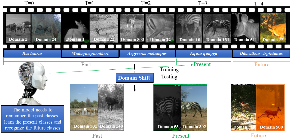
Figure 1: DACZSL setting built on iWildCam [4, 25]: The model learns a new class of animal at each time step. The model is trained such that it performs well on new target domains making the model domain invariant (Not correlating an animal with its location). The model also performs well on unseen species. The goal of this method is to improve the models deployed in the wild to avoid overfitting to background and distracting elements in the scene and also to identify new species that the model previously unseen.

1 Introduction

Human are able to accumulate knowledge from diverse visual context and integrate them over their lifetime. For example, we can recognize a first-seen wild animal and even infer their properties only by learning the related animals from cartoons watched in our childhood. Over the decades, machine learning community tries to design visual system facilities with human ability and apply them to potential real world problems to eliminate human labor, such as the above example of biological classification problem [3, 57].

According to [53], our planet has an estimated 8.7 million species, and some of them become extinct even before being studied by human. Thus it is crucial to develop visual system to help accelerate research on understanding these species. However, designing visual system models these images in the wild can be challenging [55]. For example, images of animals are often taken by camera traps deployed in locations. Some animals may frequently visit specific specific locations, which may cause the model to recognize the animal by the background of the scene rather than the animal itself. Furthermore, there are migratory animals that require the system to recognize them in new environments or locations. As shown in Fig. 1, the top right of the figure (Domain 12) shows an image of a deer in normal weather, while the bottom right (Domain 500) illustrates a deer during a California wildfire. Furthermore, models are expected to identify a species that has evolved to exist in a new environment without having a bias toward its previous environment [3, 4]. Therefore, we expect a helpful AI model that is capable to recognize seen and unseen species under seen and unseen locations and environments.

Humans are capable of recognizing unseen classes in new environments or domains. In this paper, our goal is to develop a similar AI skill that can recognize unseen classes in unseen domains. We believe that developing these AI skills over time toward real-world scale may enable accelerating species discovery with experts in the loop, as shown in Fig. 1. Images of animals are often taken by camera traps deployed in locations, which may cause the model to overfit to the background of the scene rather than the animal due to the frequent visit of that animal to that certain location. Additionally, new animals may appear over time, and a desirable model is expected to remember past animals as well as provide accurate predictions of unseen animals appearing at the same or a different location/domain.

To solve such type of tasks, we seek to develop a deep learning algorithm to continually recognize unseen classes in unseen domains. To achieve this, a desirable model needs to capture three skills: Zero-Shot Learning (ZSL), Domain Generalization (DG), and Continual Learning (CL). ZSL focuses on recognizing the unseen categories with a model trained on seen classes only [13, 11, 19]. DG, on the other hand, aims to classify the seen classes from an unseen target domain [48, 17, 52]. Along with ZSL and DG, CL pays special attention to learning a model that can handle sequential tasks without forgetting knowledge from previous tasks [7, 28, 2, 9].

We propose a generalized and unified transfer learning setting: Domain Aware Continual Zero-Shot Learning (DACZSL). Several existing works study variations of Zero-Shot Learning (ZSL), Domain Generalization (DG), and Continual Learning (CL) [32, 51]. However, when these methods are applied to the DACZSL setting, they fail to perform for three reasons.

• First, the text representation techniques used in these methods, such as Word2Vec representation [35] pre-trained from Google Corpus, are limited and do not provide discriminative guidance to recognize very similar classes. For example, classes like Parakeet auklet and Crested auklet may have collapsed representations in the Word2Vec space.

• Second, training a classifier or mapping the image features into the text class space makes classification in a challenging scenario like DACZSL very hard. Instead, a better protocol like an attribute prototypical mapping network [63] can be more effective.

• Third, existing methods are not specially designed for DACZSL with the classification of seen and unseen categories and unseen domains sequentially as the guiding goal. These issues are very severe in the challenging DACZSL problem.

To address these issues, we made the following design choices. Inspired by large-scale vision-language models such as CLIP [43] and ALIGN [22], we adopt Transformer [56] to extract text representation of class names. This provides better text grounding while eliminating the use of a classifier by replacing it with an attribute prototypical mapping pipeline [63]. We adopt CLIP pre-trained encoders as a backbone and fine-tune them with contrastive learning (Sec. 4.3) to learn robust representations of class names. To improve the representative property of each prompt, we use class-wise learnable prompts [70]. To resolve the last issue, we combine all designs mentioned above along with an adversarial knowledge disentanglement scheme (Sec. 4.2). We call our method Domain-Invariant CZSL Network (DIN).

Contributions. Our paper can be summarized as: First, we propose Domain Aware Continual Zero-Shot learning (DACZSL), which is a step towards real-world recognition challenges exploring the limits of machine understanding of unseen classes in unseen domains continually. Second, we designed a novel DACZSL method named DIN and show through comprehensive experiments that our method can significantly improve the performance compared with state-of-the-art methods carefully adapted to DACZSL from related settings. Finally, our work is the first to explore the transfer ability in scenarios with domain and unseen category gaps and sequential learning settings of large pre-trained models from vision-language pairs.

2 Related Works

Here we focus on the most relevant works related to Continual ZSL and ZSL with Large-Scale Pretraining. However, we will provide a brief introduction to the fundamental blocks, including ZSL, DG, and CL in the supplementary.

2.1 Continual Zero-Shot Learning

Early works in Continual Zero-Shot Learning (CZSL) focused on defining the problem and formulating the setting, as seen in Chaudhry et al. [7], Wei et al. [59], and Skorokhodov et al. [51]. The first paper to consider continual zero-shot performance was A-GEM [7], which randomly split the CUB and AWA datasets into 20 subsets of classes and reported zero-shot accuracy for each task sequentially. Wei et al. [59] proposed a different CZSL setting called lifelong ZSL, where the model first learns from all the seen classes from many datasets sequentially in a continual learning setting and then evaluates all the unseen classes with the learned model. In contrast, Skorokhodov et al. [51] proposed a generalized CZSL setting that extends the classification space to cover all tasks, where the model has to recognize unseen/seen classes sequentially. Most sequential CZSL methods follow Skorokhodov et al. [51] and aim to achieve better performance on more extensive feature-level attribute-based datasets, as seen in Gautam et al. [15] and Ghosh et al. [16]. Gautam et al. [15] proposed a replay-based Variational Autoencoder (VAE) to mitigate catastrophic forgetting, which led to good performance. On the other hand, Ghosh et al. [16] used stacked VAEs with the generative replay of seen samples to achieve better performance.

2.2 ZSL with Large-Scale Pretraining

In standard zero-shot learning (ZSL), image features are often extracted using pre-trained ResNet101 [20] on the ImageNet-1K dataset [44] for attribute-based datasets, and VGG [50] for text-based datasets. Similarly, the corresponding semantic class features are processed with Glove [41] or Skip-Gram [36]. However, this design has limitations as low-dimensional text features from naive Glove or Skip-Gram may not distinguish classes well in ZSL. Additionally, training visual and semantic encoders alone may not capture vision-language relationships accurately as ZSL is a visual-semantic alignment problem. Recently, pre-trained models from large vision and language pairs such as CLIP [43] and ALIGN [22] have shown promising transfer learning ability on out-of-distribution data. CLIP collaboratively pre-trains the visual encoder and the Transformer [56] text encoder on over 400 million vision and language pairs. Following works focused on fine-tuning the CLIP model to make it adaptive to more scenarios [60, 70]. In CoOp [70], CoCoOp [71] and CPL [21], learnable prompt strategies are applied to have better semantic representations. Our method uses CLIP pre-trained weights as the backbone and follows the contrastive prototypical classification design, optimizing the attribute prototypical network [63] with contrastive learning.

3 Problem Definition

In this section, we introduce the formulation of DACZSL and its related settings. Firstly, we recap Domain-Aware ZSL (Sec. 3.1), which was first proposed in CuMix [32]. Subsequently, we extend this setting to a more general one, which we call Generalized Domain-Aware ZSL. This setting involves classifying images from both unseen and seen categories. To bridge the gap between our work and previous literature, we introduce standard DACZSL (Sec. 3.2). We refer to this as uniform DACZSL, where all source domains are accessible during training for each task. Furthermore, we define non-uniform DACZSL, in which images from some domains are randomly dropped for each task, making the training non-uniform over seen domains.

3.1 Domain-Aware ZSL

Assume we have $N^{d}$ domains $\{\mathcal{D}_{i}\}$ and let $\mathcal{D}=\cup_{i=1}^{N^{d}}\mathcal{D}i$. DAZSL aims to train on source domain $\mathcal{D}^{s}\subseteq\mathcal{D}$ and test on target domain $D^{t}=\mathcal{D}\setminus\mathcal{D}^{s}$. DAZSL [32] is a two-task problem with a training step and a testing step. During training, we have access to $\mathcal{H}_{s^{d}}=\{(X_{s}^{d},Y_{s},A_{s})\},d\in{\mathcal{D}^{s}}$, where $X_{s}^{d}$, $Y_{s}$, and $A_{s}$ represent the training image set, their corresponding label set, and the semantic description set, respectively. It is worth noting that the semantic description is orthogonal to domains. During the testing step, we are provided with $X_{u}^{d},d\in\mathcal{D}_{i}$. Our objective is to learn a mapping function $f:{X}_{u}^{d}\to{Y}_{u}$, where ${Y}_{u}$ represents the label set of unseen classes.

3.2 DACZSL: Domain-Aware Continual ZSL

For DACZSL, we aim at recognizing images from unseen categories in unseen domains sequentially over $T$ tasks. We first define the training set at task $t\in\{1\cdots T\}$ to be $\mathcal{H}^{d}_{t}=\{X_{t}^{d},Y_{t},A_{t}\}$, where $X_{t}^{d},Y_{t},A_{t}$ are the training image set, their corresponding label set, and the semantic description set at task $t$ from domain $d$, $d\in\mathcal{D}_{t}$, which are all available source domains. $\mathcal{D}_{t}\subseteq\mathcal{D}^{s}$. Noticed different variations of DACZSLs have different space of $\mathcal{D}_{t}$. We proposed two DACZSL variants/settings, uniform and non-uniform that differ only during training.

Uniform DACZSL ($\mathcal{D}_{t}\equiv\mathcal{D}^{s}$). We have uniform access to training data from all sources domains $\mathcal{D}^{s}$ at task $t$.

Non-Uniform DACZSL ($\mathcal{D}_{t}\subseteq\mathcal{D}^{s}\setminus\mathcal{D}_{t}^{\operatorname{rand}}$). We randomly remove $\mathcal{D}_{t}^{\operatorname{rand}}$ from all source domains $\mathcal{D}^{s}$ at task $t$. Non-Uniform DACZSL is more challenging as we need to make our model creatively alleviate the bias of two invisible domains (one is the unseen target domain while another is the randomly removed source domain).

4 Method

4.1 Class-wise Learnable Prompts

Learning suitable prompts has been extensively studied in natural language processing to generate better text descriptions [49, 23, 69, 27]. However, the use of prompts in multi-modal scenarios, such as vision and language modalities, is less explored. Inspired by CoOp [70] and considering DACZSL as a vision-language learning problem, we propose a class-wise learnable prompt to enhance the relationship between images and the language describing the classes. This is illustrated in the top-left part of Fig. 2. DIN++ is the two-stage method with class-wise prompts learning procedure and DIN is the single-stage version without it. In contrast to CoOp, we train the learnable prompts over images from different domains, making the model more generalized and capable of capturing domain-invariant class-specific knowledge.

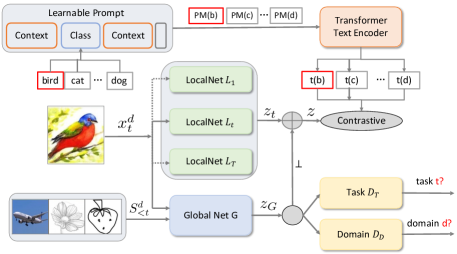
Figure 2: This figure depicts the architecture of our proposed DIN and DIN++ method, which involves two key steps. First, we use contrastive learning to create a class-wise prompt by combining the output $t(\texttt{CLASS})$ from the CLIP pre-trained Transformer text encoder with the output $z_{G}$ from the global network $G$, using prompt $\operatorname{PM}(\texttt{CLASS})$. Remarkably, this step requires no access to any information from the local networks.Next, we employ adversarial contrastive learning between $t(\texttt{CLASS})$ and the concatenated output $z$ from both the global and local networks. This ensures that the global network solely outputs domain and task-invariant information, resulting in better visual-language paired information representation by the text and visual encoders. Notably, it is worth mentioning that the standard DIN method does not involve the first prompt learning step.

Our prompt for class $c$ is formulated as follows:

$$\text{PM}(c)=[W]_{1\to k_{1}}\ \ [\texttt{CLASS}]\ \ [W]_{k_{1}+1\to k_{2}}[\texttt{EOS}],$$ (1)

where $[W]{i},i\in[1,k_{2}],0\leq k_{1}\leq k_{2}$ represents the learnable context, which is the semantic embedding of word $W$. In our experiments, we use a 512-dimensional representation for each context. We consider two variants of where to add the class token, either in the middle ($k_{2}=2k_{1}$) or at the end of the prompt ($k_{1}+1=k_{2}$, meaning $[W]_{k_{1}+1\to k_{2}}$ is not used). The difference between these variants is minor, as shown in the experimental results in Fig. 3, so we adopt the simpler option.

To train the class-wise learnable prompt, we randomly sample $H_{t}\in\mathcal{H}_{t}$ satisfying $\|H^{d}_{c}\|=K,c\in\mathcal{S}_{t},H_{c}^{d}\in H_{t}$, where $K$ is the number of samples per domain and per class. We input $\text{PM}{(c)}$ to the Text Encoder and use the global net G to learn this prompt by contrastive learning. Notably, we do not consider local nets $L_{i},i\in[1,T]$ for prompt learning, as shown in Fig. 2. Here, $t(\cdot)=\operatorname{Text(PM(\cdot))}$.

4.2 Adversarial Knowledge Disentanglement

We aim to extract distribution-invariant knowledge from domain- and task-specific information through visual representation. Let $x_{t}^{d}\in X_{t}^{d}$ represent an image from domain $d$ and task $t$ with label $c$ (see Fig.2). We process this image through Local Nets $L(\cdot)$ and Global Net $G(\cdot)$, where $L(\cdot)$ is instantiated for each task $t\in{1,\cdots,T}$ to learn task-variant information, while we push the Global Net $G(\cdot)$ to learn task and domain-invariant knowledge. In practice, we may optionally store a small set of samples from previously seen tasks, denoted as $S^{d}_{<t},d\in\mathcal{D}^{s}$, where $\mathcal{D}^{s}$ represents source domains. To encourage the features in the global network to be independent of every task-variant local net, we design a disentangled loss inspired by[5] and shown in Eqn. 2.

$$\mathcal{L}_{\text{disen}}(z_{t\in\mathcal{T}},z_{G})=\sum_{t=1}^{T}\|\langle z_{t},z_{G}\rangle\|^{2}.$$ (2)

To make the knowledge in the global net $G$ task and domain-invariant, we adopt an adversarial training scheme inspired by ACL [10]. Analogous to the GAN pipeline, the global network can be seen as a generator. We design two discriminators: the task discriminator $D_{T}$ evaluates which task the generated sample is from, while the domain discriminator $D_{D}$ classifies the domain of the current sample, as shown in Eqn. 3.

$$\mathcal{L}_{\text{adv}} (G,D_{T},D_{D})=$$ (3)

$$\alpha\min_{G}\max_{D_{T}}\mathrm{E}_{x_{t}^{d}\sim P(X_{\mathcal{T}}^{\mathcal{D}})}\sum_{t=1}^{T}y_{t}^{d}\log(D_{T}(G(x_{t}^{d})))$$

$$+\beta\min_{G}\max_{D_{D}}\mathrm{E}_{x_{t}^{d}\sim P(X_{\mathcal{T}}^{\mathcal{D}})}\sum_{d=1}^{D}y_{t}^{d}\log(D_{D}(G(x_{t}^{d}))).$$

Our method differs from ACL [10] by employing two classification heads solely for domain and task classification. Unlike ACL, we don’t use discriminators to identify real or fake samples. Our integrated adversarial learning of these heads is more challenging to train and optimize compared to the identification head in ACL. Additionally, our approach is tailored to ZSL settings and multimodal vision-language learning setups, whereas ACL is not designed for such tasks.

4.3 Contrastive Fine-tuning

In contrast to traditional classification-based pipelines in CL, DG, and ZSL, we adopt a more natural and proper contrastive prototypical classifier. To achieve this, we use a contrastive loss, as shown in Eqn. 4, which encourages the mapped feature representation of the outputs from the local nets and the global net, denoted by ${z}=f(z_{t},z_{G})$, to be closer to the label text feature representation ${t}_{i}$ of the same class, and farther from those of different classes.

$$\mathcal{L}_{\text{cont}}=-\log\frac{\exp\left(\operatorname{r}\left({t}_{i},{z}\right)/\tau\right)}{\sum_{k=1}^{N}\exp\left(\operatorname{r}\left({t}_{k},{z}\right)/\tau\right)},$$ (4)

Here, $N$ represents the number of samples in the current batch, and $\tau$ is the temperature parameter. The function $\operatorname{r}\left(\cdot,\cdot\right)$ computes the cosine similarity between the two input feature representations. By minimizing the contrastive loss, we encourage the features to be closer to the corresponding label text feature, which helps to learn a more effective feature representation that can generalize well to new tasks and domains.

Total Loss. To learn class-level prompts, we employ $K$-shot fine-tuning on training images, where $K$ denotes the number of samples per class per domain for each task. For updating the rest of the networks, including the global and local networks, text encoder, and discriminators, we design our loss function as follows:

$$\mathcal{L}_{\text{DIN}}=\lambda_{1}\mathcal{L}_{\text{disen}}+\lambda_{2}\mathcal{L}_{\text{adv}}+\lambda_{3}\mathcal{L}_{\text{cont}},$$ (5)

where $\lambda_{1}$, $\lambda_{2}$, and $\lambda_{3}$ are hyperparameters that control the influence of different loss components. The disentangled loss $\mathcal{L}_{\text{disen}}$ encourages the features in the global network to be independent of every task-variant local net, while the adversarial loss $\mathcal{L}_{\text{adv}}$ makes the knowledge in the global net task and domain-invariant. The contrastive loss $\mathcal{L}_{\text{cont}}$ is used for the class-level prompt learning. For more details and the algorithm, please refer to the supplementary.

5 Experiments

Evaluation Metrics.

In order to verify the efficiency of our methods, we use comprehensive evaluation metrics for DACZSL. These include last seen accuracy (LS), mean seen accuracy (mS), mean unseen accuracy (mU), and the harmonic mean of seen and unseen (mH), as well as forgetting rate (BWT) accumulated over task time steps for DACZSL. The formal definitions can be found in the supplementary.

Baselines.

To compare the performance of our proposed method, we design strong baselines by adapting state-of-the-art (SOTA) methods from related areas.

• CuMix [32] and its variants. CuMix was the first paper to consider the combination of ZSL and DG, which we refer to as the DAZSL setting. The key idea is to mix up learning signals by sampling three images; two images are from the same domain and the third is from a different domain.

• CNZSL [51] and its variants. CNZSL is the state-of-the-art method in embedding-based ZSL and one of the best-performing methods in continual ZSL. This approach applies a simple but effective class normalization strategy in ZSL and CZSL, showing significant improvements.

• BDCZSL [26] and IGCZSL [67]: BDCZSL employs a bi-directional incremental alignment loss mechanism, which enables dynamic adaptation to the introduction of new classes. On the other hand, the latest research in IGCZSL introduces a semantically-guided generative random walk loss, aiming to enhance the recognition of unseen classes.

Implementation Details

For all our experiments, we use ResNet-50 [20] backbone by default for fair comparisons. The domain discriminator and the task discriminator all use 3-layer MLPs. We use AdamW [31] for optimization. We use the default hyperparameters for the baselines but search for important ones using the validation set. More implementation details can be found in the supplementary.

5.1 Introduced Benchmarks.

Our experiments are conducted on two benchmarks: the DomainNet dataset [40] and the iWildCam dataset [4] provided by the Wilds benchmark [25].

DomainNet CZSL. DomainNet is originally designed for multi-source domain adaptation and contains around $0.6$ million images from 345 classes and 6 domains. We use the noise-reduced version of the dataset with 4 domains [46]. For DAZSL, we select 45 classes as unseen classes for testing, matching the number used in [54]. We follow the same training/validation split as CuMix [32]: 245 seen classes for training and the remaining 55 for validation. Initially, there is no attribute information for each class, so we use word2vec embeddings [35] extracted from Google News corpus to obtain a 300-dimensional representation of each class and adopt $L2$ normalization afterward. We also provide a version with text features from a Transformer [56] pre-trained by CLIP [43]. For DACZSL, we randomly split DomainNet into 8 tasks, each containing 43 classes. We removed the last class to make each task contain an equal number of classes since an imbalanced number of classes over tasks can make the model unstable.

iWildCam CZSL. To get closer to real-world applications of DACZSL, we use the iWildCam dataset [4] provided by the Wilds benchmark [25]. We use the in-domain split as the source domain and the out-of-domain split as the target domain. The locations of the camera trap are treated as domains. Source domains consist of 243 camera trap locations, and target domains consist of 48 camera trap locations. We split the 312 classes into 7 tasks, each containing 26 classes, for continual learning.

Method	Sketch			Clipart			Painting			Avg.
	LS$\uparrow$	mH$\uparrow$	BWT$\uparrow$	LS$\uparrow$	mH$\uparrow$	BWT$\uparrow$	LS$\uparrow$	mH$\uparrow$	BWT$\uparrow$	LS$\uparrow$	mH$\uparrow$	BWT$\uparrow$
CuMix [32]	6.97 / 5.39	3.58 / 3.08	0.15 / 0.20	6.32 / 5.81	3.11 / 2.95	0.24 / -0.15	6.80 / 5.35	3.47 / 2.98	0.09 / 0.22	6.70 / 5.52	3.39 / 3.00	0.16 / 0.09
CuMix w/o Mixup	2.67 / 2.61	1.92 / 1.88	-0.03 / 0.00	2.36 / 2.34	1.63 1.61	0.02 / -0.03	2.80 /2.72	2.01 / 2.72	-0.05 / -0.08	2.61 / 2.58	1.85 / 1.80	-0.02 / -0.04
CuMix + Tf	9.52 / 6.94	4.06 / 3.91	0.32 / 0.13	10.25 / 9.30	4.09 / 4.06	0.33 / 0.28	9.57 / 8.60	4.69 / 4.51	0.06 / -0.41	9.78 / 8.28	4.28 / 4.16	0.24 / 0.00
CNZSL [51]	6.68 / 6.37	2.52 / 2.36	-0.66 / -0.45	6.40 / 5.94	2.79 / 2.75	-0.71 / -0.46	7.82 / 6.89	2.09 / 1.98	-0.27 / -0.48	6.97 / 6.40	2.47 / 2.36	-0.55 / -0.46
CNZSL w/o CN	7.16 / 3.22	2.67 / 1.42	-0.75 / -0.65	7.07 / 3.92	2.92 / 1.63	-0.72 / -0.10	8.36 / 3.87	2.15 / 1.61	-0.35 / -0.53	7.53 / 3.67	2.58 / 1.55	-0.61 / -0.43
CNZSL + Tf	45.74 / 41.20	31.75 / 28.59	1.00 / 0.89	54.19 / 48.43	37.33 / 28.73	1.17 / 2.93	59.15 / 52.39	40.37 / 34.5	0.96 / 1.26	53.03 / 47.34	36.48 / 30.61	1.04 / 1.69
BDCZSL [26]	15.62 / 10.34	6.98 / 4.98	-15.54 / -7.50	16.61 / 8.62	7.60 / 4.96	-16.45 / -8.80	15.96 / 7.88	7.69 / 4.86	-17.54 / -7.56	16.06 / 8.95	7.42 / 4.93	-16.51 / -7.95
BDCZSL + Tf	33.20 / 19.15	28.51 / 16.93	-0.46 / 4.68	39.69 / 25.59	36.39 / 24.14	-4.13 / 2.15	54.95 / 42.09	51.82 / 40.39	-2.89 / 1.28	42.61 / 28.94	38.91 / 27.15	-2.49 / 2.70
IGCZSL [67]	33.42 / 28.01	12.81 / 9.71	-28.01 / -11.80	36.93 / 28.86	14.46 / 10.78	-32.83 / -12.49	39.16 / 26.13	15.66 / 10.33	-30.85 / -12.12	36.51 / 27.66	14.31 / 10.27	-30.56 / -12.14
IGCZSL + Tf	26.36 / 26.63	23.14 / 23.42	1.49 / 6.00	29.21 / 30.68	27.27 / 28.56	0.73 / 5.65	54.15 / 45.73	51.51 / 44.07	1.03 / 0.52	36.57 / 34.35	33.97 / 32.02	1.08 / 4.06
CLIP-ZSL [43]	21.39	20.83	0.00	27.73	27.46	0.00	63.06	62.35	0.00	37.39	36.88	0.00
CLIP-FT	60.17 / 58.98	60.23 / 60.01	0.60 / 0.25	67.04 / 65.77	67.18 / 66.49	0.41 / 0.00	61.51 / 61.56	62.00 / 61.33	0.29 / 1.02	62.91 / 62.10	63.14 / 62.61	0.43 / 0.42
DIN	74.20 / 71.45	61.64 / 57.98	1.07 / 2.03	82.15 / 79.69	70.00 / 68.43	1.15 / 2.29	77.16 / 72.52	75.74 / 73.66	1.95 / 0.47	77.84 / 74.55	69.13 / 66.69	1.39 / 1.60
DIN++	74.53 / 70.99	63.78 / 60.14	0.92 / 0.81	81.31 / 76.01	71.24 / 69.18	1.12 / 0.65	76.00 / 71.19	76.10 / 71.96	1.82 / 1.55	77.28 / 72.73	70.37 / 67.09	1.29 / 1.00

Table 1: Comparative results on DomainNet-CZSL in uniform and non-uniform settings. In each cell, left is the uniform result while right is non-uniform result. + Tf means we use CLIP [43] pre-trained text Transformer as the feature extractor. We use ResNet50 [20] as visual encoder backbone for fair evaluations.

Method	LS$\uparrow$	mH$\uparrow$	BWT$\uparrow$
CuMix + Tf [32]	11.56	3.24	-0.18
CNZSL + Tf [51]	34.34	19.98	-24.35
BDCZSL + Tf [26]	25.81	7.56	-6.51
IGCZSL + Tf [67]	32.30	3.29	-21.35
CLIP-ZSL [43]	9.21	8.27	0.00
CLIP-FT [43]	36.01	14.22	-42.38
DIN	54.70	27.56	-16.37
DIN++ (Ours)	42.62	36.47	-13.48

Table 2: Comparative results on iWildCam-CZSL [4] dataset, based on domain splits defined iWildCam benchmark  [25].

5.2 DACZSL Experimental Analysis

Compared to DAZSL, DACZSL is designed to recognize images from both unseen domains and unseen categories sequentially, making it more general and natural. In Table 1, we provide comparative results for uniform DACZSL and non-uniform DACZSL (uniform results are shown on the left, while non-uniform results are on the right in each cell). We present two variants of our DIN model: one is a single-stage model without prompt learning and uses the default prompt (i.e., ”An image of a [CLS]”), denoted as DIN, and the other variant is a learnable prompt model called DIN++. Our approach significantly outperforms the SOTA methods in related approaches, such as CNZSL [51] and CuMix [32], along with their variants, in the DACZSL setting. The contrastive prototypical classifier in DACZSL is more dynamic and natural compared to the approach of training an extra classifier in CuMix. Additionally, a powerful text representation is essential for learning the relationship between image-text pairs. We observe significant improvements when using Transformer features instead of Word2Vec as the text representation for CuMix and CNZSL. Our network, which uses CLIP as a backbone, achieves significantly boosted results compared to the raw CLIP model (CLIP-ZSL) and fine-tuned CLIP with contrastive learning (CLIP-FT). We believe that fine-tuning on the DACZSL setting with a CLIP backbone using contrastive prototypical learning is highly valuable and contributes to the majority of gains. Furthermore, we find that our specially designed network can significantly improve performance, as shown in our ablation studies.

Non-uniform DACZSL, where all the images in several randomly selected domains are removed during training, is more challenging than uniform DACZSL because we need to consider transferring knowledge from imbalanced and limited sources. As shown in the right part of each cell in Table 1, our method demonstrates a clear improvement over all baselines. Moreover, when comparing uniform and non-uniform DACZSL results, our method is robust to randomly removed-domain bias with smaller relevant drops, and our performance remains stable in both settings. However, baseline methods show clear drops from uniform DACZSL to non-uniform DACZSL.

In the iWildCam-CZSL [4] benchmark, we tested the baselines with CLIP Transformer extracted features. The results of these experiments, presented in Table 2, demonstrate that our method significantly outperforms the other baselines in sequentially classifying species. Our method’s higher mH shows that it performs better at predicting unseen species.

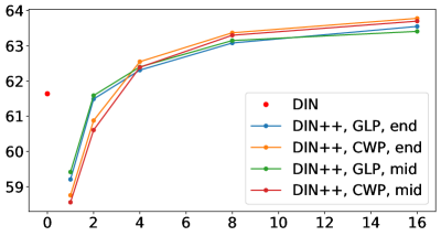
Figure 3: Harmonic mean of seen and unseen accuracy of DIN with prompts on target domain sketch. GLP represents general learnable prompts while CWP means class-wise prompts. end and mid represents two positions to place class labels in a prompt.

5.3 Ablation Studies

In this section, we conduct a comprehensive ablation analysis of our proposed DIN on the uniform DACZSL setting in the DomainNet-CZSL benchmark. Our method comprises several main components, including the global module, local modules, discriminators for domains and tasks, learnable prompt module, memory rehearsal, and disentanglement loss. We perform ablation studies on each of these components to evaluate their individual contributions to our approach.

Learnable Prompts.

CLIP [43] provides a standard prompt (i.e., a fixed text description) template: “A picture of a CLASS”. However, this fixed template may not be an optimal representation for a complex task like DACZSL. To address this issue, we introduced class-level learnable prompts and conducted an ablation study, as shown in Fig. 3. Specifically, we compared Global Learnable Prompts (GLP) over all classes with Class-Wise Prompts (CWP). We found that using learnable prompts after fine-tuning on increasing samples per class per domain led to a steady increase in harmonic mean accuracy. We also observed that the performance difference between class positions mid and end was marginal.

Besides, after fine-tuning on 16 examples per class per domain, we found that CWP outperforms GLP by 0.37%. Therefore, we conducted further analysis on the simpler end form and class-wise learnable prompt. As prompt learning makes our method a two-stage one, we denote the method with prompt learning as a variant of DIN, called DIN++. In Table 1, we demonstrate that adding a class-wise learnable prompt can result in a more balanced classification performance (e.g., mH using learnable prompts increases 2.14% on the clipart target domain).

Memory Rehearsal.

To optimize memory usage, we focused on minimal memory requirements for each task, storing only one sample per domain per class. Our results, as seen in Tab. 4 comparing #a with #d, reveal a 2.26% / 2.21% improvement in LS/mH with a single memory rehearsal. Additional ablation studies with more samples are detailed in the supplementary material. We observed steady performance gains when increasing memory from 1 to 4 examples. Beyond this, the benefit of expanding memory rehearsal from 4 to 16 examples is slight. This is partly because our LocalNets-GlobalNet coherent module effectively retains knowledge from previous tasks, preventing catastrophic forgetting. This module’s efficacy in maintaining high classification accuracy, coupled with our model’s ability to learn efficiently from a small number of rehearsal samples, highlights its efficiency.

Global and Local Modules.

We design the global network to store domain-invariant and task-invariant knowledge, while using the local networks to process all task-variant data. We conduct a cumulative ablation study on our method DIN in the scenario with one memory rehearsal. The results are shown in Tab. 4. Comparing #a2 with #a1, we can observe that adding Local Nets can significantly improve LS by 7.53%, which means less forgetting. More importantly, adding LocalNets can help us achieve positive knowledge transfer over tasks (e.g., the forgetting rate BWT increases from 0.51 to 0.65).

#	Module	LS$\uparrow$	mS$\uparrow$	mU$\uparrow$	mH$\uparrow$	BWT$\uparrow$
a	DIN (Ours)	77.84	78.91	62.19	69.13	1.39
b	- memory	75.56	77.66	61.01	67.87	1.21
c1	- w/o DD	76.92	77.35	61.83	68.72	0.81
c2	- w/o DT	75.63	76.91	60.37	67.64	1.20
d	- w/o DD+DT	75.58	76.56	59.44	66.92	0.79

Table 3: Ablation studies on memory rehearsal and adversarial training averaging over all target domains.

#	G	L	Adv	Disen	LS$\uparrow$	mH$\uparrow$	BWT$\uparrow$
a1	✓				64.22	64.81	0.51
a2	✓	✓			71.75	65.44	0.65
a3	✓		✓		26.62	28.87	-13.08
a4	✓	✓	✓		76.34	68.17	0.61
a5	✓	✓		✓	75.58	66.92	0.79
a6	✓	✓	✓	✓	77.84	69.13	1.39

Table 4: Cumulative ablation study on our method DIN with $1$-memory rehearsal. We report the average performance by traversing all target domains.

Adversarial Learning and Disentanglement.

Adversarial learning and disentangled learning signals are essential to create a global network that contains domain-invariant and task-invariant information. Unlike traditional adversarial training, we only consider two classification tasks, one to classify the domain and another to classify the task. Fake samples are not generated and are not necessary in our case. Our objective is to train the global network to output domain-invariant and task-invariant information that the discriminators cannot distinguish.

We conducted an ablation study on the impact of adversarial training and disentanglement loss on our method’s performance. Results are shown in Table 4. Specifically, we observe that when adversarial loss is removed, the LS and mH performance drops by 2.26% and 2.21%, respectively (comparing #a2 to #a5 and #a4 to #a6). When the disentanglement loss is removed, we observe marginal improvement in performance (#a2 vs. #a4 and #a5 vs. #a6).

We also compared our method’s performance with and without considering domain and task invariant features. Results in Table 4 #a3 show that adding the adversarial loss without local networks leads to a significant performance drop by 37.6% LS and 35.94% mH. The forgetting rate also drops by 13.59. This indicates that domain and task invariant features are important for storing essential domain/task independent information, but they cannot be directly applied to classify images from different domains and categories sequentially, which leads to catastrophic forgetting after adversarial training.

We also studied the impact of removing the domain and task discriminators separately. Results in Table 4 show that the accuracy over all metrics is more influenced by the task discriminator (LS/mH drops by 0.92%/0.41% vs. 2.21%/1.49% after removing DD/DT), while the domain discriminator contributes more to make the global network more robust with less forgetting (BTW drops by 0.58 vs. 0.19 after removing DD vs. DT).

Finally, we analyzed the impact of our proposed disentanglement loss. Our results show that the disentanglement loss can improve the performance marginally but not strongly. Overall, our ablation study demonstrates the importance of both adversarial training and disentanglement loss in our proposed method for DACZSL.

5.4 Global Network Latent Feature Analysis

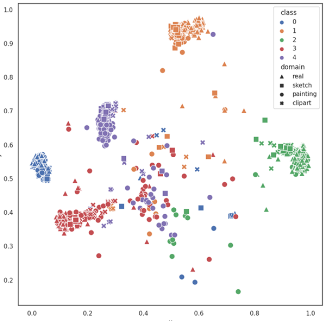
Figure 4: t-SNE visualization of latent features from the global network post-training for DomainNet-CZSL task 1, showcasing 5 classes for analysis.

During our exploration of DomainNet-CZSL task 1, we trained a global network and analyzed its latent feature extraction, as depicted in Figure 4. The figure uses distinct colors and shapes to represent individual classes and domain-specific features, respectively. Our findings affirm that the global network adeptly identifies and extracts class-specific and domain-invariant features, a critical requirement for effective generalized ZSL.

Notably, we observed that features within the same class cluster closely, maintaining clear separation from features of different classes. This clustering pattern signifies the network’s proficiency in discerning class-specific attributes. Furthermore, the convergence of features from varied domains within the same class underscores the network’s ability to extract domain-invariant characteristics. This skill in distilling domain-invariant features is pivotal for the network’s performance in generalizing to new, unseen domains in zero-shot learning scenarios.

6 Conclusion

In this paper, we introduced the Domain-Aware Continual Zero-Shot Learning (DACZSL) task, which addresses the challenge of recognizing images from unseen categories and domains in a lifelong learning setting. Through the example of species classification in camera-trap images, we demonstrated the relevance of this problem. We proposed two new benchmarks for the domain-aware continual zero-shot learning task, DomainNet-CZSL and iWildCam-CZSL, and presented a novel contrastive prototypical knowledge disentangled representation network. Our experiments showed that a more representative text feature extractor improves performance on extreme out-of-distribution images, and that disentangling domain-invariant and task-invariant information is important for achieving promising results. We hope that this work will facilitate future research into knowledge transfer in out-of-distribution settings and lead to better vision-language models that can understand the relationships between the seen and unseen continually. Additionally, we believe that the models developed in this setting can serve as a foundation for studying animals in the real world, where online distribution shifts and unseen classes are naturally encountered.

Appendix A Complementary Related Works

Here we provide a brief introduction of related works to the fundamental blocks, including Zero-Shot Learning, Domain Generalization and Continual Learning.

(Generalized) Zero-Shot Learning.

Zero-Shot Learning (ZSL) is a machine learning problem that aims to recognize images of objects from unseen categories using models trained only on images from seen classes. ZSL has been widely adopted in the computer vision community as a benchmark for evaluating the transfer learning ability of models. In recent years, a more complex but realistic setting called Generalized Zero-Shot Learning (GZSL) has been proposed [62]. GZSL extends the ZSL setting by considering the scenario where images from both seen and unseen categories are present at testing time. The larger classification space in GZSL makes the problem more challenging. Existing ZSL approaches can be broadly classified into embedding-based and generative-based methods [62]. Embedding-based methods learn an alignment between different modalities (e.g., visual and semantic) directly for classification [29, 51, 64]. Generative-based methods focus on synthesizing realistic unseen-class images with unseen text features [38, 66] or generating images that are creatively deviating from seen classes [72, 11, 58, 12]. In our work, we propose a method that combines both embedding-based and generative-based approaches for GZSL. We aim to learn a joint representation space that can capture the common structure between visual and semantic modalities and generate realistic samples for unseen classes. By doing so, we hope to improve the accuracy of GZSL models, especially for unseen classes that are similar to seen ones.

Domain Generalization.

Domain Generalization (DG) is an important problem in computer vision, where the aim is to recognize images from an unseen target domain with a machine learning model trained on source domains. This problem has been studied extensively in the context of animal classification, as it is a common problem encountered in this domain [3, 4]. Recently, the Wilds benchmark has been proposed to study wild domain shifts encountered in the real world [25]. One of the key objectives in DG is to train a model on source domains and then evaluate the model on the target domain. Hence, a crucial question to improve the model generation ability is how to disentangle domain-invariant representations from domain-specific ones [8, 18, 68, 42]. Several approaches have been proposed to address this problem. For example, Ding et al.[8] proposed to learn a separate domain-specific network for each domain and a shared domain-invariant network to capture global information shared across domains. Meanwhile, Mitrovic et al.[37] proposed a self-supervised learning scheme to obtain an optimal classifier that minimizes the representation variance over different domains. In contrast to these approaches, our work considers disentangling domain-invariant information not only from different domains but also from variant tasks learned continually. This is an important problem, as models trained on multiple tasks can suffer from catastrophic forgetting when they are evaluated on new tasks [39]. Therefore, our work aims to address this issue by developing a disentangled representation learning framework that can effectively learn domain-invariant features across multiple tasks and domains.

Continual Learning.

Continual Learning (CL) is the ability of a machine learning model to learn new tasks sequentially with distribution bias, without forgetting previously learned tasks [34, 33]. One of the main challenges in CL is catastrophic forgetting, which refers to a significant drop in a learner’s performance when transitioning from a trained task to a new one, as the model may forget the knowledge learned from previous tasks. Memory-based and structure-based methods are the most relevant approaches to our work. Memory-based methods sample representative data from previous tasks and replay them to avoid forgetting them. However, efficiently sampling the most representative data is crucial for achieving good performance [30, 6, 7, 61, 28]. Another approach to alleviate catastrophic forgetting is to expand the network progressively to have more task-dependent parameters. In this way, partial parameters from previous seen tasks are kept or minimally changed to achieve good performance on seen classes [45, 47, 65].

Appendix B Training Details and Algorithms

B.1 Architecture and Training Details

Our proposed method, DIN/DIN++, incorporate several key components, including a class-wise learnable prompt, a global network, local networks, a domain discriminator, and a task discriminator. In the following sections, we will provide more detailed explanations of the training and optimization strategies for each module. Additionally, we have included the code for our method as a supplementary resource.

Class-Wise Learnable Prompt Module.

This is a key component of our proposed method. Previous work such as CLIP [43] used a naive prompt in the form of ”An image of a [CLASS],” which may not capture class-specific information across different datasets. Zhou et al.[70] demonstrated that a more tailored prompt for a specific dataset could significantly improve classification accuracy on unseen data. Building on this insight, we propose a domain-invariant class-wise learnable prompt module. The general form of the learnable prompt is described in Eqn. 4 of the main paper. The initialization methods for the General Learnable Prompt (GLP) and Class-Wise Prompt (CWP) differ. Our prompt module is represented as a tensor of shape (# classes, prompt length, dim per prompt), with GLP initializing each class tensor to be identical, while CWP initializes each class tensor uniquely. We train the prompt module by accessing $K$-training examples per class and domain, with a learning rate of 0.002 and $K$ set to 16 by default. For experiments with different values of $K$, we train for 200 epochs for 16/8, 100 epochs for 4/2, and 50 epochs for 1. We use a batch size of 256 for all experiments, including baselines and methods, along with their variants[43, 70].

Global and Local Coherent Module.

This module is another important component of our proposed method. We use ResNet50 [20] pre-trained from CLIP [43] as the visual encoder for both the global and local networks. However, the global network is designed to store domain and task-invariant information, while the local networks are designed to process task-variant information from different source domains. We adopt the Transformer [56] as the text encoder, pre-trained from CLIP. The learning rate for these modules is set to 5e-7. We use the AdamW optimizer [31] and set the warmup length to 5 and weight decay to 0.02. Additionally, we use the cosine learning scheduler to adapt the learning rate. We set the training epochs for all our modules to 25.

Domain and Task Discriminators.

They are also crucial components of our proposed method. For both discriminators, we use 3-layer MLPs incorporated with LeakyReLU activation. The learning rate is set to 0.001, and weight decay is set to 0.01. We use SGD for optimization, and the latent dimension of the discriminators is set to 1024. Similar to ACL [10], we add the Gradient Reversal layer [14] before feeding the generated latent features by the global network to the domain and task-specific discriminators.

CuMix/CNZSL and Their Variants.

We conduct ablation experiments to validate critical hyperparameters and mainly use the default best hyperparameters provided. For CuMix [32], we set the hyperparameters of the best-performing model on DACZSL and related experiments to have an image mixup weight of 0.001, feature mixup weight of 0.5, mixup step of 2, and mixup beta of 2. The backbone learning rate is set to 0.0001, and the mapping network learning rate is set to 0.001, with weight decay of 0.00005. The training epoch is set to 25. For CNZSL [51], we adopt the same design and apply task-specific class normalization. For CuMix, CNZSL, and their variants using Transformer, which is pre-trained from CLIP [43], to extract the text features, we set the epoch equal to 50. We notice that for CNZSL and its related experiments, we set the batch size to 512, while we set the batch size to 360 for CuMix related experiments due to limited memory.

B.2 Training Algorithm

We present the whole training algorithm of our method at Alg. 1 and the prompt learning algorithm at Alg. 2.

Algorithm 1 Domain-Invariant Continual Zero-Shot Learning Network (DIN)

0:  Training set $\mathcal{H}_{s}=\sum_{d}\mathcal{H}_{s}^{d}=\{X_{s}^{d},Y_{s}^{d},A_{s}^{d}\},d\in\overline{\mathcal{D}_{i}}$, few-shot $k_{1}$, buffer sampling $k_{2}$, batch size $n_{b}$, total task $T$, prompt learning epoch $E_{1}$, main model epoch $E_{2}$, $\theta_{\operatorname{pr}},\theta_{\operatorname{Text}},\theta_{G},\theta_{L},\theta_{D_{dm}},\theta_{D_{ta}}$

  Memory Buffer $\mathbb{B}\leftarrow\{\}$

  Randomly split $\mathcal{H}_{s}^{d}=\sum_{t}\mathcal{H}_{t}^{d},t\in[1,T]$, then current visible classes $\mathcal{S}_{t}$

  for $t=1$ to $T$ do

     Run prompt learning Algorithm. 2

     Unfreeze $\theta_{G},\theta_{L},\theta_{\operatorname{Text}},\theta_{D_{dm}},\theta_{D_{ta}}$

     Freeze $\theta_{\operatorname{pr}}$

     for $e_{2}=1$ to $E_{2}$ do

        Compute $\mathcal{L}_{\operatorname{adv}}$ (Eqn. 5) for $G$ using $H_{t}\cup\mathbb{B}$

        Compute $\mathcal{L}_{\operatorname{disen}}$ (Eqn. 6) using $f_{\theta},S$

        Compute contrastive loss $\mathcal{L}_{\operatorname{cont}}$ (Eqn. 7) using $f_{\theta},\operatorname{Text}$

        $\mathcal{L}=\lambda_{1}\mathcal{L}_{\text{disen}}+\lambda_{2}\mathcal{L}_{\text{adv}}+\lambda_{3}\mathcal{L}_{\text{cont}}$

        $\theta_{G}\leftarrow\theta_{G}-\alpha_{G}\nabla\mathcal{L}$

        $\theta_{L}\leftarrow\theta_{L}-\alpha_{L}\nabla\mathcal{L}$

        $\theta_{\operatorname{Text}}\leftarrow\theta_{\operatorname{Text}}-\alpha_{\operatorname{Text}}\nabla\mathcal{L}$

        for $i=1$ to $n_{d}$ do

           Compute $\mathcal{L}_{\operatorname{adv}}$ (Eqn. 5) for $D_{dm}$ and $D_{ta}$ using $H_{t}\cup\mathbb{B}$

           $\theta_{D_{dm}}\leftarrow\theta_{D_{dm}}-\alpha_{D_{dm}}\nabla\mathcal{L}$

           $\theta_{D_{ta}}\leftarrow\theta_{D_{ta}}-\alpha_{D_{ta}}\nabla\mathcal{L}$

        end for

        Random sampling $k_{2}$ samples per class as $\mathbb{B}_{t}$

        $\mathbb{B}\leftarrow\mathbb{B}\cup\mathbb{B}_{t}$

     end for

  end for

Algorithm 2 Class-Wise Prompt Learning

  for $t=1$ to $T$ do

     Freeze $\theta_{G},\theta_{L},\theta_{\operatorname{Text}},\theta_{D_{dm}},\theta_{D_{ta}}$

     Unfreeze $\theta_{\operatorname{pr}}$

     $f_{\theta}=f(\theta_{G})$

     for $e_{1}=1$ to $E_{1}$ do

        Randomly sample $H_{t}\in\mathcal{H}_{t}\vdash\|H^{d}_{c}\|=k_{1},c\in\mathcal{S}_{t},H_{c}^{d}\in H_{t}$

        Compute contrastive loss $\mathcal{L}_{\operatorname{cont}}$ (Eqn. 7) using $f_{\theta},\theta_{\operatorname{Text}}$

        $\theta_{\operatorname{pr}}\leftarrow\theta_{\operatorname{pr}}-\alpha_{\operatorname{pr}}\nabla\mathcal{L}_{\operatorname{cont}}$

     end for

  end for

Noticed in the main paper, we denote the method without class-wise prompt learning as DIN, a single-stage model. We denote the setting with the learnable prompt as DIN++.

B.3 iWildCam DACZSL Setting (Complementary)

We design the iWildCam-CZSL benchmark using the version of iWildCam provided by the Wilds [25] benchmark. Dataset consists of 181 different animal species and extra class indicating empty scene. The location of the camera traps are regarded as domains. The total amount of samples found in the dataset is 203,029. We divide the dataset into 7 tasks. Each task introduces 26 classes to the model. The dataset has a predefined domain split for training and evaluation. The training domain split contains 243 camera traps. The testing domain split consists of 48 different camera traps. Since each class does not have images captured from all the possible domains, DACZSL on top of iWildCam-CZSL is naturally a non-uniform setting. We consider each as source and target in our DACZSL setting.

Appendix C Illustration of Related Settings

C.1 Setting Differences

Figure 5: Our DACZSL problem: we illustrate here the difference between Zero-Shot Learning (ZSL), Continual ZSL (CZSL), and our Domain-Aware CZSL (DACZSL). CZSL learning is class incremental zero-shot learning. In DACZSL, the model is tested on a different target domain than the one used to train.

C.2 ZSL, DG, and CL

We begin with a conceptual analysis of fundamental settings that are most relevant to our work, namely Zero-Shot Learning (ZSL), Domain Generalization (DG), and Continual Learning (CL). We illustrate the differences between these settings in Fig. 6. ZSL and DG both involve training on the source domain $H_{1}$. The primary difference between the two is the type of out-of-distribution cases encountered during testing. In ZSL, we aim to recognize images from unseen categories but seen domains in $H_{2}$. Conversely, in DG, we aim to recognize images from unseen domains but seen categories. In the case of CL, the images are from the same domain and same class. However, this setting poses a sequential task learning problem, where the goal is to minimize forgetting of the previous tasks $H_{1\to T-1}$.

Figure 6: Conceptual differences between Zero-Shot Learning (ZSL), Domain Generalization (DG), and Continual Learning (CL).

ZSL, DG, and CL are fundamental settings but not enough to solve our key focus: recognizing images from unseen categories and unseen domains in a life-long setting. Next, we present some existing settings that are related to us.

C.3 (Generalized) Domain-Aware ZSL

Figure 7: Intuitions of Domain-Aware Zero-Shot Learning (DAZSL). Generalized DAZSL is an extended version to recognize images not only from unseen classes but also from seen categories.

Suppose we have 3 domains ( $d_{1}$, $d_{2}$, and $d_{3}$), 6 classes ($c_{i},i\in\mathbb{Z},i\in[1,6]$). We denote the $c_{1}\to c_{4}$ as the training set while the rest as the testing set. GDAZSL will consider recognizing images from both seen and unseen classes while ZSDG will only care about recognizing images from unseen categories. We show setting intuitions at Fig. 8.

Figure 8: (Generalized) Domain-Aware Zero-Shot Learning Setting.

C.4 Continual ZSL

We show the intuition of CZSL at Fig. 9.

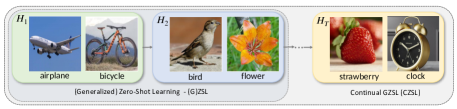
Figure 9: Intuition of Continual Zero-Shot Learning (CZSL).

C.5 Domain-Aware Continual ZSL (DACZSL)

In Fig. 10, we show intuition of DACZSLs, which recognizes images from unseen domains and unseen categories sequential. Sequential figures are also presented in the main content Fig. 1.

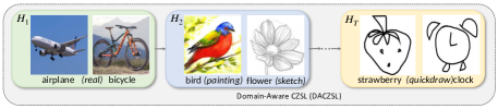
Figure 10: Intuition of Domain-Aware Continual Zero-Shot Learning.

Here we consider several variants of DACZSL, which are Domain-Agonistic Continual Zero-Shot Learning (DAgCZSL), Uniform Domain-Aware Continual Zero-Shot Learning (U-DACZSL), and Non-Uniform Domain-Aware Continual Zero-Shot Learning (N-DACZSL). The formal definition of U-DACZSL and N-DACZSL have been provided in the main content. Here we show the conceptual differences with examples among those settings.

Suppose we have 3 domains ( $d_{1}$, $d_{2}$, and $d_{3}$), 6 classes ($c_{i},i\in\mathbb{Z},i\in[1,6]$) uniformly divided into 3 sequential tasks. We first propose the Domain Agnostic Continual Zero-Shot Learning; visualized at Fig. 11.

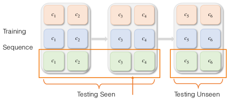
Figure 11: Domain-Agnostic Continual Zero-Shot Learning (DAgCZSL).

Later we present domain-aware (uniform) CZSL, which is more interesting; visualized at Fig. 12.

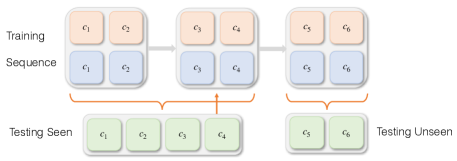
Figure 12: Uniform Domain-Aware Continual Zero-Shot Learning.

Next, we consider a more difficult task domain-sensitive (non-uniform) CZSL, in which one seen domain is randomly removed in training; visualized at Fig. 13.

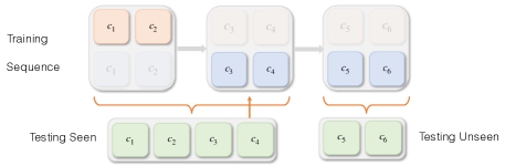
Figure 13: Non-Uniform Domain-Aware Continual Zero-Shot Learning.

Appendix D DAZSL Results and Analysis

D.1 Generalized Analysis

We have illustrated the concept of Domain-Aware Zero-Shot Learning (DAZSL) and Generalized Domain-Aware Zero-Shot Learning (GDAZSL) setting in the main text and Section. C.3 in this supplementary. Here we provide more details. We first present the statistics of benchmark DomainNet [40]. Then we provide more statistical results.

D.2 Statistics of DomainNet for (G)DAZSL

The pioneering work combining zero-shot learning and domain generalization is CuMix [32]. We even further consider a more difficult case with the combination of generalized zero-shot learning with domain generalization. We call the first setting DAZSL while the latter as Generalized DAZSL (GDAZSL). We first show the statistics at Fig. 5. For DAZSL, in the testing step, we only consider the test split consisting of 45 classes. However, in GDAZSL, we take all testing images over 345 classes into considerations.

setting	# classes	quick	sketch	info	clip	paint	real	total.
train	245	85, 750	33, 803	27, 050	23, 238	36, 816	86, 480	293, 137
val	55	19, 250	7, 690	4, 651	5, 891	6, 324	17, 528	61, 334
test	45	22, 500	9, 626	6, 195	6, 317	10, 418	24, 155	79, 211
total	345	127, 500	51, 119	37, 896	35, 446	53, 558	128, 163	433, 682

Table 5: DomainNet [40] statistics for DAZSL and GDAZSL. After getting the best hyper-parameters on the validation set, train and val will be merged as the training set in practice.

D.3 Evaluation Metrics for (G)DAZSL

Mean Seen Accuracy (mSA) is the seen accuracy over tasks:

$$\operatorname{mSA}=\frac{1}{C^{s}}\sum_{c=1}^{C^{s}}\frac{\#\operatorname{correct\ pred.\ in\ c}}{\#\operatorname{samples\ in\ c}}$$ (6)

Mean Unseen Accuracy (mUA) is the unseen accuracy over tasks:

$$\operatorname{mUA}=\frac{1}{C^{u}}\sum_{c=1}^{C^{u}}\frac{\#\operatorname{correct\ pred.\ in\ c}}{\#\operatorname{samples\ in\ c}}$$ (7)

Mean Harmonic (mH) over mSA and mUA:

$$\operatorname{mH}=\frac{2\operatorname{mSA}\times\operatorname{mUA}}{\operatorname{mSA}+\operatorname{mUA}}$$ (8)

Seen-Unseen Area Under Curve (SUAUC) is to detect model’s bias towards seen or unseen data. We first build a classification rule as follows:

$$\hat{y}=\text{argmax}_{c\in(C^{s}\cup C^{u})}\ \ f_{c}(\textbf{x}-\gamma\mathbb{I}[c\in C^{s}])$$ (9)

where $\mathbb{I}[\cdot]\in\{0,1\}$ is the seen mask and $\gamma$ is called as the calibration factor. With $\gamma$ from $-\infty$ to $+\infty$, we calculate a set of seen accuracy and unseen accuracy to form $\mathbf{s}$ and $\mathbf{u}$. We compute the area to be SUAUC.

D.4 DAZSL Results and Analysis

The pioneer work in combining ZSL and DG is CuMix [32]. In the testing step, the searching space is only unseen classes. Therefore, their setting can be regarded as the combination of DG and ZSL, which we denote as DAZSL. We show the results at Tab. 6. Our proposed method also achieved significantly better results than baselines.

Method	quick	sketch	info	clip	paint	Avg.
Source-only LB	9.81	25.04	17.43	26.49	28.5	21.45
Oracle UB	14.62	30.25	20.58	28.00	29.81	24.65
CuMix∗ [32]	9.9	22.6	17.8	27.6	25.5	20.68
CuMix [32]	8.7	21.8	17.0	26.2	24.9	19.72
CNZSL [51]	9.11	26.12	16.64	28.08	29.98	21.99
CLIP-ZSL [43]	1.55	22.71	35.51	22.91	57.46	28.03
DIN (Ours)	10.93	40.67	47.85	51.88	56.60	41.59

Table 6: DAZSL experimental results. All results are the average after three trials with the same setting. ^∗ means the reported results. LB is the lower bound while UB is the upper bound. We use ResNet50 [20] as the default backbone.

D.5 GDAZSL Results and Analysis

We utilized state-of-the-art (SOTA) and popular methods from related areas, such as ZSL [51] and DG [32], and transplanted them to the domain adaptation ZSL (DAZSL) setting. CuMix [32] is the only method that focuses on DAZSL setting and provides public implementation. We fine-tuned the key hyperparameters of these baselines on the validation set and evaluated their performance on the extended and more challenging setting, named Generalized DAZSL (GDAZSL). In GDAZSL, the prediction space includes the union of seen and unseen classes in unseen domains, which is more general and challenging than DAZSL in [32]. We report the results of the baselines on GDAZSL in Table 7, where we show the metrics harmonic mean (mH) and area under seen-unseen curve score (mAUC). The LB denotes the lower bound where we naively train on the source domains and test on the target domain, while the UB is the performance of the model trained and tested on the target domain.

We used the same network architecture as CNZSL [51] for LB and UB. Since GDAZSL is not a sequential learning task, we provided a variant of our method by removing the private network and the task discriminator. Our proposed method significantly outperformed the baselines by a large margin, as shown in Table 7. Interestingly, we even outperformed the expected upper bound on almost all metrics, which we attribute to better training protocols and architecture design. We report the complete results at Tab. 8.

Method	Sketch		Clipart		Painting		Avg
	mH	mAUC	mH	mAUC	mH	mAUC	mH	mAUC
Source-only (LB)	18.80	9.05	23.03	12.52	23.97	11.75	21.93	11.11
Oracle (UB)	19.73	14.82	19.13	17.44	25.89	18.06	21.58	16.77
CNZSL [51]	20.30	9.84	22.98	12.97	23.64	12.10	22.31	11.64
CuMix [32]	4.63	10.33	4.47	11.98	7.20	12.07	5.43	11.46
CLIP-ZSL [43]	9.99	2.18	11.22	2.72	34.48	20.60	18.56	8.50
DIN (Ours)	33.53	18.32	40.61	24.36	33.85	17.04	36.00	19.91

Table 7: GDAZSL experimental results. We show significantly better results than baselines. Moreover, we also find that our proposed DIN can achieve better results than Oracle (UB), in which unseen images from unseen domains are used for training and uses the same network architecture as the one in CNZSL.

Method	quick				sketch				info				clip				paint				Avg.
	mS	mU	mH	mAUC	mS	mU	mH	mAUC	mS	mU	mH	mAUC	mS	mU	mH	mAUC	mS	mU	mH	mAUC	mS	mU	mH	mAUC
Source-only (LB)	7.93	3.33	4.69	0.61	38.4	12.4	18.80	9.05	16.88	9.51	12.14	2.69	47.56	15.2	23.03	12.52	42.14	16.76	23.97	11.75	30.58	11.44	16.53	7.32
Oracle (UB)	54.68	5.08	9.28	6.37	54.61	12.05	19.73	14.82	29.57	9.38	14.23	5.91	66.98	11.17	19.13	17.44	61.32	16.42	25.89	18.06	53.43	10.82	17.65	12.52
CNZSL [51]	7.85	3.87	5.19	0.63	39.2	13.7	20.30	9.84	17.5	9.53	12.34	2.80	48.15	15.1	22.98	12.97	43.82	16.19	23.64	12.10	31.30	11.68	16.89	7.67
CuMix [32]	10.9	0.23	0.58	0.68	47.99	2.43	4.63	10.33	21.52	0.59	1.15	3.01	53.11	2.33	4.47	11.98	49.67	3.88	7.20	12.07	36.64	1.91	3.61	7.61
CLIP-ZSL [43]	0.33	0	0	0.37	10.55	9.47	9.99	2.18	21.00	16.77	18.65	7.00	12.73	10.04	11.22	2.72	37.28	32.07	34.48	20.60	16.38	13.67	14.87	6.57
DIN (Ours)	4.63	1.95	2.75	4.43	34.43	32.67	33.53	18.32	29.56	28.91	29.23	14.24	41.73	39.54	40.61	24.36	31.40	36.71	33.85	17.04	28.35	27.96	27.99	15.68

Table 8: GDAZSL complete experimental results.

D.6 DAZSL vs. GDAZSL

Combining Tab. 6 and Tab. 8, we show that GDAZSL is a much difficult setting compared with DAZSL reflected by the performance over all metrics by all experimented methods. We found that our method can achieve significantly better results by a large margin.

Appendix E DACZSL Complemantary Results

E.1 Evaluation Metrics

We present here the evaluation matrices for DACZSL, and refer to the supplementary for DAZSL and GDAZSL matrices. Inspired by standard continual learning literature, we compute the seen accuracy after training at the last task:

$$\operatorname{LS}=\frac{1}{T}\sum_{t=1}^{T}\operatorname{Acc}(X_{t}^{d}|\mathcal{M}_{T}),\quad d\in\mathcal{D}_{i}.$$ (10)

where $\mathcal{D}_{i}$ is the target domain and $\mathcal{M}_{t}$ is the model trained till step $t$. $\operatorname{Acc}(X_{t}^{d}|\mathcal{M}_{T})$ is the classification accuracy on image set $X^{d}_{t}$ with the model trained till task $T$. We also compute the mean seen and unseen accuracy over tasks:

$$\operatorname{mS} =\frac{1}{T}\sum_{t=1}^{T}\sum_{k=1}^{t}\operatorname{Acc}(X_{k}^{d}|\mathcal{M}_{t})$$ (11)

$$\operatorname{mU} =\frac{1}{T-1}\sum_{t=1}^{T-1}\sum_{k=t+1}^{T}\operatorname{Acc}(X_{k}^{d}|\mathcal{M}_{t}).$$

We consider the harmonic mean mH of mS and mU to exam how balance the method is over seen and unseen accuracy. mH is defined as $2\operatorname{mS}\cdot\operatorname{mU}/(\operatorname{mS}+\operatorname{mU})$.

Besides, we also consider the measure of forgetting rate:

$$\operatorname{BWT}=\sum_{t=1}^{T}\operatorname{Acc}(X_{t}^{d}|\mathcal{M}_{T})-\operatorname{Acc}(X_{t}^{d}|\mathcal{M}_{t}).$$ (12)

E.2 Compare with CL Methods

Our proposed DACZSL setting involves zero-shot learning (ZSL), continual learning (CL), and domain generalization (DG), so we consider existing works with different combinations of them. Therefore, we adopt the following baselines: CuMix (DG+ZSL) and CNZSL (CL+ZSL). Unfortunately, we can not find open-sourced existing works on CL+DG. We believe that exploring CL papers in our setting improves our experiments section. So we attached the results of EWC [24] and MAS [1] in Tab. 9. The results show that our proposed method performs significantly better than EWC and MAS.

Method	LS$\uparrow$	mS$\uparrow$	mU$\uparrow$	mH$\uparrow$	BWT$\uparrow$
EWC [24]	8.49	9.25	3.43	4.92	0.81
EWC [24] + Tf	50.31	51.86	26.19	34.57	0.55
MAS [1]	7.82	9.07	2.88	4.21	1.01
MAS [1] + Tf	51.23	52.89	27.61	36.08	0.94
DIN (Ours)	74.20	77.26	51.28	61.64	1.07

Table 9: Comparison with adaptive continual learning methods of noise-reduced DomainNet. + Tf means we use CLIP [43] pre-trained text Transformer. We report the average over all possible target domains.

E.3 Full Ablation Table

Let us recap the total loss to optimize our model (main text Sec. 4.3 Eqn. 5)

$$\mathcal{L}_{\text{DIN}}=\lambda_{1}\mathcal{L}_{\text{disen}}+\lambda_{2}\mathcal{L}_{\text{adv}}+\lambda_{3}\mathcal{L}_{\text{cont}},$$ (13)

where the hyperparameters $\lambda_{1}$, $\lambda_{2}$, and $\lambda_{3}$ control the influence of different loss components in our model. The disentangled loss ($\mathcal{L}{\text{disen}}$) encourages the features in the global network to be independent of every task-variant local network, while the adversarial loss ($\mathcal{L}{\text{adv}}$) promotes task and domain-invariant knowledge in the global network. The contrastive loss ($\mathcal{L}_{\text{cont}}$) is used for class-level prompt learning.

We conducted extensive experiments to determine the optimal values of $\lambda_{1}$, $\lambda_{2}$, and $\lambda_{3}$, and report the results with the best hyper-parameters we were able to achieve. As a complementary analysis to Table 5 in the main paper, we present the results of our component analysis in Tab. 10. What distinguishes our study from Table 5 in the main paper is that we performed an ablation study by removing the contractive loss ($\mathcal{L}_{\text{cont}}$), which demonstrates a significant drop in performance when visual-language pairs are learned without contractive learning. These findings suggest that strong language-guided DACZSL is necessary to better understand the relationships between visual and language domains.

$\mathcal{L}_{\text{disen}}$	$\mathcal{L}_{\text{adv}}$	$\mathcal{L}_{\text{cont}}$	# in Tab. 5	LS$\uparrow$	mH$\uparrow$	BWT$\uparrow$
✓			-	20.16	18.61	0.09
	✓		-	31.97	30.05	0.31
		✓	a2	71.75	65.44	0.65
✓	✓		-	34.22	31.69	1.02
	✓	✓	a4	76.34	68.17	0.61
✓		✓	a5	75.58	66.92	0.79
✓	✓	✓	a6	77.84	69.13	1.39

Table 10: Ablation study on our proposed DIN with $1$-memory rehearsal. # in Tab. 5 represents which experimental setting in the main paper Table 5 is the same as the one listed. We report the average performance by leveraging all target domains.

References

- Aljundi et al. [2018] Rahaf Aljundi, Francesca Babiloni, Mohamed Elhoseiny, Marcus Rohrbach, and Tinne Tuytelaars. Memory aware synapses: Learning what (not) to forget. In Proceedings of the European Conference on Computer Vision (ECCV), pages 139–154, 2018.
- Aljundi et al. [2019] Rahaf Aljundi, Klaas Kelchtermans, and Tinne Tuytelaars. Task-free continual learning. In Proceedings of the IEEE/CVF Conference on Computer Vision and Pattern Recognition, pages 11254–11263, 2019.
- Beery et al. [2018] Sara Beery, Grant Van Horn, and Pietro Perona. Recognition in terra incognita. In Proceedings of the European conference on computer vision (ECCV), pages 456–473, 2018.
- Beery et al. [2021] Sara Beery, Arushi Agarwal, Elijah Cole, and Vighnesh Birodkar. The iwildcam 2021 competition dataset. arXiv preprint arXiv:2105.03494, 2021.
- Bousmalis et al. [2016] Konstantinos Bousmalis, George Trigeorgis, Nathan Silberman, Dilip Krishnan, and Dumitru Erhan. Domain separation networks. Advances in neural information processing systems, 29:343–351, 2016.
- Castro et al. [2018] Francisco M Castro, Manuel J Marín-Jiménez, Nicolás Guil, Cordelia Schmid, and Karteek Alahari. End-to-end incremental learning. In Proceedings of the European conference on computer vision (ECCV), pages 233–248, 2018.
- Chaudhry et al. [2018] Arslan Chaudhry, Marc’Aurelio Ranzato, Marcus Rohrbach, and Mohamed Elhoseiny. Efficient lifelong learning with a-gem. arXiv preprint arXiv:1812.00420, 2018.
- Ding and Fu [2017] Zhengming Ding and Yun Fu. Deep domain generalization with structured low-rank constraint. IEEE Transactions on Image Processing, 27(1):304–313, 2017.
- Ebrahimi et al. [2020a] Sayna Ebrahimi, Mohamed Elhoseiny, Trevor Darrell, and Marcus Rohrbach. Uncertainty-guided continual learning with bayesian neural networks. ArXiv, abs/1906.02425, 2020a.
- Ebrahimi et al. [2020b] Sayna Ebrahimi, Franziska Meier, Roberto Calandra, Trevor Darrell, and Marcus Rohrbach. Adversarial continual learning. In Computer Vision–ECCV 2020: 16th European Conference, Glasgow, UK, August 23–28, 2020, Proceedings, Part XI 16, pages 386–402. Springer, 2020b.
- Elhoseiny and Elfeki [2019] Mohamed Elhoseiny and Mohamed Elfeki. Creativity inspired zero-shot learning. In Proceedings of the IEEE/CVF International Conference on Computer Vision, pages 5784–5793, 2019.
- Elhoseiny et al. [2021] Mohamed Elhoseiny, Kai Yi, and Mohamed Elfeki. Cizsl++: Creativity inspired generative zero-shot learning. arXiv preprint arXiv:2101.00173, 2021.
- Farhadi et al. [2009] Ali Farhadi, Ian Endres, Derek Hoiem, and David Forsyth. Describing objects by their attributes. In 2009 IEEE Conference on Computer Vision and Pattern Recognition, pages 1778–1785. IEEE, 2009.
- Ganin and Lempitsky [2015] Yaroslav Ganin and Victor Lempitsky. Unsupervised domain adaptation by backpropagation. In International conference on machine learning, pages 1180–1189. PMLR, 2015.
- Gautam et al. [2020] Chandan Gautam, Sethupathy Parameswaran, Ashish Mishra, and Suresh Sundaram. Generalized continual zero-shot learning. arXiv preprint arXiv:2011.08508, 2020.
- Ghosh [2021] Subhankar Ghosh. Dynamic vaes with generative replay for continual zero-shot learning. arXiv preprint arXiv:2104.12468, 2021.
- Gong et al. [2019] Rui Gong, Wen Li, Yuhua Chen, and Luc Van Gool. Dlow: Domain flow for adaptation and generalization. In Proceedings of the IEEE/CVF Conference on Computer Vision and Pattern Recognition, pages 2477–2486, 2019.
- Gulrajani and Lopez-Paz [2020] Ishaan Gulrajani and David Lopez-Paz. In search of lost domain generalization. In International Conference on Learning Representations, 2020.
- Han et al. [2021] Zongyan Han, Zhenyong Fu, Shuo Chen, and Jian Yang. Contrastive embedding for generalized zero-shot learning. arXiv preprint arXiv:2103.16173, 2021.
- He et al. [2016] Kaiming He, Xiangyu Zhang, Shaoqing Ren, and Jian Sun. Deep residual learning for image recognition. In Proceedings of the IEEE conference on computer vision and pattern recognition, pages 770–778, 2016.
- He et al. [2022] Xuehai He, Diji Yang, Weixi Feng, Tsu-Jui Fu, Arjun Akula, Varun Jampani, Pradyumna Narayana, Sugato Basu, William Yang Wang, and Xin Eric Wang. Cpl: Counterfactual prompt learning for vision and language models. arXiv preprint arXiv:2210.10362, 2022.
- Jia et al. [2021] Chao Jia, Yinfei Yang, Ye Xia, Yi-Ting Chen, Zarana Parekh, Hieu Pham, Quoc V. Le, Yun-Hsuan Sung, Zhen Li, and Tom Duerig. Scaling up visual and vision-language representation learning with noisy text supervision. In ICML, 2021.
- Jiang et al. [2020] Zhengbao Jiang, Frank F Xu, Jun Araki, and Graham Neubig. How can we know what language models know? Transactions of the Association for Computational Linguistics, 8:423–438, 2020.
- Kirkpatrick et al. [2017] James Kirkpatrick, Razvan Pascanu, Neil Rabinowitz, Joel Veness, Guillaume Desjardins, Andrei A Rusu, Kieran Milan, John Quan, Tiago Ramalho, Agnieszka Grabska-Barwinska, et al. Overcoming catastrophic forgetting in neural networks. Proceedings of the national academy of sciences, 114(13):3521–3526, 2017.
- Koh et al. [2021] Pang Wei Koh, Shiori Sagawa, Henrik Marklund, Sang Michael Xie, Marvin Zhang, Akshay Balsubramani, Weihua Hu, Michihiro Yasunaga, Richard Lanas Phillips, Irena Gao, Tony Lee, Etienne David, Ian Stavness, Wei Guo, Berton Earnshaw, Imran Haque, Sara M Beery, Jure Leskovec, Anshul Kundaje, Emma Pierson, Sergey Levine, Chelsea Finn, and Percy Liang. Wilds: A benchmark of in-the-wild distribution shifts. In Proceedings of the 38th International Conference on Machine Learning, pages 5637–5664. PMLR, 2021.
- Kuchibhotla et al. [2022] H. Kuchibhotla, S. S. Malagi, S. Chandhok, and V. N. Balasubramanian. Unseen classes at a later time? no problem. In 2022 IEEE/CVF Conference on Computer Vision and Pattern Recognition (CVPR), pages 9235–9244, Los Alamitos, CA, USA, 2022. IEEE Computer Society.
- Le Scao and Rush [2021] Teven Le Scao and Alexander M Rush. How many data points is a prompt worth? In Proceedings of the 2021 Conference of the North American Chapter of the Association for Computational Linguistics: Human Language Technologies, pages 2627–2636, 2021.
- Lee et al. [2019] Kibok Lee, Kimin Lee, Jinwoo Shin, and Honglak Lee. Overcoming catastrophic forgetting with unlabeled data in the wild. In Proceedings of the IEEE/CVF International Conference on Computer Vision, pages 312–321, 2019.
- Liu et al. [2020] Shaoteng Liu, Jingjing Chen, Liangming Pan, Chong-Wah Ngo, Tat-Seng Chua, and Yu-Gang Jiang. Hyperbolic visual embedding learning for zero-shot recognition. In Proceedings of the IEEE/CVF Conference on Computer Vision and Pattern Recognition, pages 9273–9281, 2020.
- Lopez-Paz and Ranzato [2017] David Lopez-Paz and Marc’Aurelio Ranzato. Gradient episodic memory for continual learning. Advances in neural information processing systems, 30:6467–6476, 2017.
- Loshchilov and Hutter [2017] Ilya Loshchilov and Frank Hutter. Decoupled weight decay regularization. arXiv preprint arXiv:1711.05101, 2017.
- Mancini et al. [2020] Massimiliano Mancini, Zeynep Akata, Elisa Ricci, and Barbara Caputo. Towards recognizing unseen categories in unseen domains. In proceedings of the European Conference on Computer Vision. Springer, 2020.
- McClelland et al. [1995] James L McClelland, Bruce L McNaughton, and Randall C O’Reilly. Why there are complementary learning systems in the hippocampus and neocortex: insights from the successes and failures of connectionist models of learning and memory. Psychological review, 102(3):419, 1995.
- McCloskey and Cohen [1989] Michael McCloskey and Neal J Cohen. Catastrophic interference in connectionist networks: The sequential learning problem. In Psychology of learning and motivation, pages 109–165. Elsevier, 1989.
- Mikolov et al. [2013a] Tomas Mikolov, Kai Chen, Greg Corrado, and Jeffrey Dean. Efficient estimation of word representations in vector space. arXiv preprint arXiv:1301.3781, 2013a.
- Mikolov et al. [2013b] Tomas Mikolov, Ilya Sutskever, Kai Chen, Greg S Corrado, and Jeff Dean. Distributed representations of words and phrases and their compositionality. In Advances in neural information processing systems, pages 3111–3119, 2013b.
- Mitrovic et al. [2020] Jovana Mitrovic, Brian McWilliams, Jacob C Walker, Lars Holger Buesing, and Charles Blundell. Representation learning via invariant causal mechanisms. In International Conference on Learning Representations, 2020.
- Narayan et al. [2020] Sanath Narayan, Akshita Gupta, Fahad Shahbaz Khan, Cees GM Snoek, and Ling Shao. Latent embedding feedback and discriminative features for zero-shot classification. arXiv preprint arXiv:2003.07833, 2020.
- Parisi et al. [2019] German I Parisi, Ronald Kemker, Jose L Part, Christopher Kanan, and Stefan Wermter. Continual lifelong learning with neural networks: A review. Neural networks, 113:54–71, 2019.
- Peng et al. [2019] Xingchao Peng, Qinxun Bai, Xide Xia, Zijun Huang, Kate Saenko, and Bo Wang. Moment matching for multi-source domain adaptation. In Proceedings of the IEEE/CVF International Conference on Computer Vision, pages 1406–1415, 2019.
- Pennington et al. [2014] Jeffrey Pennington, Richard Socher, and Christopher D Manning. Glove: Global vectors for word representation. In Proceedings of the 2014 conference on empirical methods in natural language processing (EMNLP), pages 1532–1543, 2014.
- Piratla et al. [2020] Vihari Piratla, Praneeth Netrapalli, and Sunita Sarawagi. Efficient domain generalization via common-specific low-rank decomposition. In International Conference on Machine Learning, pages 7728–7738. PMLR, 2020.
- Radford et al. [2021] Alec Radford, Jong Wook Kim, Chris Hallacy, A. Ramesh, Gabriel Goh, Sandhini Agarwal, Girish Sastry, Amanda Askell, Pamela Mishkin, Jack Clark, Gretchen Krueger, and Ilya Sutskever. Learning transferable visual models from natural language supervision. In ICML, 2021.
- Russakovsky et al. [2015] Olga Russakovsky, Jia Deng, Hao Su, Jonathan Krause, Sanjeev Satheesh, Sean Ma, Zhiheng Huang, Andrej Karpathy, Aditya Khosla, Michael Bernstein, et al. Imagenet large scale visual recognition challenge. International journal of computer vision, 115(3):211–252, 2015.
- Rusu et al. [2016] Andrei A. Rusu, Neil C. Rabinowitz, Guillaume Desjardins, Hubert Soyer, J. Kirkpatrick, K. Kavukcuoglu, Razvan Pascanu, and R. Hadsell. Progressive neural networks. ArXiv, abs/1606.04671, 2016.
- Saito et al. [2019] Kuniaki Saito, Donghyun Kim, Stan Sclaroff, Trevor Darrell, and Kate Saenko. Semi-supervised domain adaptation via minimax entropy. In Proceedings of the IEEE/CVF International Conference on Computer Vision, pages 8050–8058, 2019.
- Schwarz et al. [2018] Jonathan Schwarz, Wojciech M. Czarnecki, Jelena Luketina, Agnieszka Grabska-Barwinska, Y. Teh, Razvan Pascanu, and R. Hadsell. Progress & compress: A scalable framework for continual learning. ArXiv, abs/1805.06370, 2018.
- Seo et al. [2020] Seonguk Seo, Yumin Suh, Dongwan Kim, Geeho Kim, Jongwoo Han, and Bohyung Han. Learning to optimize domain specific normalization for domain generalization. In Computer Vision–ECCV 2020: 16th European Conference, Glasgow, UK, August 23–28, 2020, Proceedings, Part XXII 16, pages 68–83. Springer, 2020.
- Shin et al. [2020] Taylor Shin, Yasaman Razeghi, Robert L. Logan IV, Eric Wallace, and Sameer Singh. AutoPrompt: Eliciting knowledge from language models with automatically generated prompts. In Empirical Methods in Natural Language Processing (EMNLP), 2020.
- Simonyan and Zisserman [2015] Karen Simonyan and Andrew Zisserman. Very deep convolutional networks for large-scale image recognition. In ICLR, 2015.
- Skorokhodov and Elhoseiny [2021] Ivan Skorokhodov and Mohamed Elhoseiny. Class normalization for zero-shot learning. In International Conference on Learning Representations, 2021.
- Somavarapu et al. [2020] Nathan Somavarapu, Chih-Yao Ma, and Zsolt Kira. Frustratingly simple domain generalization via image stylization. arXiv preprint arXiv:2006.11207, 2020.
- Sweetlove [2011] Lee Sweetlove. Number of species on earth tagged at 8.7 million. Nature, 23, 2011.
- Thong et al. [2020] William Thong, Pascal Mettes, and Cees GM Snoek. Open cross-domain visual search. Computer Vision and Image Understanding, 200:103045, 2020.
- Van Horn et al. [2018] Grant Van Horn, Oisin Mac Aodha, Yang Song, Yin Cui, Chen Sun, Alex Shepard, Hartwig Adam, Pietro Perona, and Serge Belongie. The inaturalist species classification and detection dataset. In Proceedings of the IEEE conference on computer vision and pattern recognition, pages 8769–8778, 2018.
- Vaswani et al. [2017] Ashish Vaswani, Noam Shazeer, Niki Parmar, Jakob Uszkoreit, Llion Jones, Aidan N Gomez, Łukasz Kaiser, and Illia Polosukhin. Attention is all you need. In Advances in neural information processing systems, pages 5998–6008, 2017.
- Voina et al. [2021] Doris Voina, Eric Shea-Brown, and Stefan Mihalas. A biologically inspired architecture with switching units can learn to generalize across backgrounds. bioRxiv, 2021.
- Vyas et al. [2020] Maunil R Vyas, Hemanth Venkateswara, and Sethuraman Panchanathan. Leveraging seen and unseen semantic relationships for generative zero-shot learning. In European Conference on Computer Vision, pages 70–86. Springer, 2020.
- Wei et al. [2020] Kun Wei, Cheng Deng, and Xu Yang. Lifelong zero-shot learning. In Proceedings of the Twenty-Ninth International Joint Conference on Artificial Intelligence, IJCAI-20, pages 551–557, 2020.
- Wortsman et al. [2021] Mitchell Wortsman, Gabriel Ilharco, Mike Li, Jong Wook Kim, Hannaneh Hajishirzi, Ali Farhadi, Hongseok Namkoong, and Ludwig Schmidt. Robust fine-tuning of zero-shot models. arXiv preprint arXiv:2109.01903, 2021.
- Wu et al. [2019] Yue Wu, Yinpeng Chen, Lijuan Wang, Yuancheng Ye, Zicheng Liu, Yandong Guo, and Yun Fu. Large scale incremental learning. In Proceedings of the IEEE/CVF Conference on Computer Vision and Pattern Recognition, pages 374–382, 2019.
- Xian et al. [2017] Yongqin Xian, Bernt Schiele, and Zeynep Akata. Zero-shot learning-the good, the bad and the ugly. In Proceedings of the IEEE Conference on Computer Vision and Pattern Recognition, pages 4582–4591, 2017.
- Xu et al. [2020] Wenjia Xu, Yongqin Xian, Jiuniu Wang, Bernt Schiele, and Zeynep Akata. Attribute prototype network for zero-shot learning. In 34th Conference on Neural Information Processing Systems. Curran Associates, Inc., 2020.
- Yi et al. [2022] Kai Yi, Xiaoqian Shen, Yunhao Gou, and Mohamed Elhoseiny. Exploring hierarchical graph representation for large-scale zero-shot image classification. In European Conference on Computer Vision, pages 116–132. Springer, 2022.
- Yoon et al. [2018] Jaehong Yoon, Eunho Yang, Jeongtae Lee, and Sung Ju Hwang. Lifelong learning with dynamically expandable networks. ArXiv, abs/1708.01547, 2018.
- Yue et al. [2021] Zhongqi Yue, Tan Wang, Qianru Sun, Xian-Sheng Hua, and Hanwang Zhang. Counterfactual zero-shot and open-set visual recognition. In Proceedings of the IEEE/CVF Conference on Computer Vision and Pattern Recognition, pages 15404–15414, 2021.
- Zhang et al. [2023] Wenxuan Zhang, Paul Janson, Kai Yi, Ivan Skorokhodov, and Mohamed Elhoseiny. Continual zero-shot learning through semantically guided generative random walks. In IEEE/CVF International Conference on Computer Vision, 2023.
- Zhao et al. [2020] Shanshan Zhao, Mingming Gong, Tongliang Liu, Huan Fu, and Dacheng Tao. Domain generalization via entropy regularization. Advances in Neural Information Processing Systems, 33, 2020.
- Zhong et al. [2021] Zexuan Zhong, Dan Friedman, and Danqi Chen. Factual probing is [mask]: Learning vs. learning to recall. In Proceedings of the 2021 Conference of the North American Chapter of the Association for Computational Linguistics: Human Language Technologies, pages 5017–5033, 2021.
- Zhou et al. [2021] Kaiyang Zhou, Jingkang Yang, Chen Change Loy, and Ziwei Liu. Learning to prompt for vision-language models. arXiv preprint arXiv:2109.01134, 2021.
- Zhou et al. [2022] Kaiyang Zhou, Jingkang Yang, Chen Change Loy, and Ziwei Liu. Conditional prompt learning for vision-language models. In Proceedings of the IEEE/CVF Conference on Computer Vision and Pattern Recognition, pages 16816–16825, 2022.
- Zhu et al. [2018] Yizhe Zhu, Mohamed Elhoseiny, Bingchen Liu, Xi Peng, and Ahmed Elgammal. A generative adversarial approach for zero-shot learning from noisy texts. In CVPR, 2018.