DeepGANTT: A Scalable Deep Learning Scheduler for Backscatter Networks

Abstract.

Novel backscatter communication techniques enable battery-free sensor tags to interoperate with unmodified standard IoT devices, extending a sensor network’s capabilities in a scalable manner. Without requiring additional dedicated infrastructure, the battery-free tags harvest energy from the environment, while the IoT devices provide them with the unmodulated carrier they need to communicate. A schedule coordinates the provision of carriers for the communications of battery-free devices with IoT nodes. Optimal carrier scheduling is an NP-hard problem that limits the scalability of network deployments. Thus, existing solutions waste energy and other valuable resources by scheduling the carriers suboptimally. We present DeepGANTT, a deep learning scheduler that leverages graph neural networks to efficiently provide near-optimal carrier scheduling. We train our scheduler with relatively small optimal schedules obtained from a constraint optimization solver, achieving a performance within 3% of the optimal scheduler. DeepGANTT generalizes to networks $6\times$ larger in the number of nodes and $10\times$ larger in the number of tags than those used for training, breaking the scalability limitations of the optimal scheduler and reducing carrier utilization by up to $50\%$ compared to the state-of-the-art heuristic. Our scheduler efficiently reduces energy and spectrum utilization in backscatter networks.

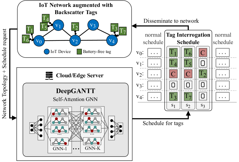
Figure 1. DeepGANTT employs GNNs to schedule wireless communications in a backscatter network. It takes a graph representing the wireless network as input and produces a schedule, which directs IoT nodes ($v$) to interrogate every battery-free tag ($\mathtt{T}$) with minimal resources by reducing the number of carriers ($\mathtt{C}$) and timeslots ($s$) needed.

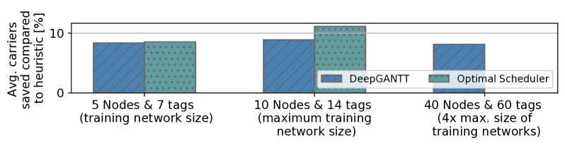
Figure 2. DeepGANTT provides near-optimal schedules and generalizes well beyond the scalability limitation of the optimal scheduler. DeepGANTT’s performance is within 3% of the optimum on trained problem sizes, but can be applied to much larger networks.

1. Introduction

Backscatter communications enable a new class of wireless devices that harvest energy from their environment to operate without batteries (Liu et al., 2013; Wang et al., 2017; Hessar et al., 2018). Recent advances have demonstrated how these battery-free backscatter devices—tags for short— can seamlessly perform bidirectional communications with unmodified Commercial Off-The-Shelf (COTS) wireless devices over standard physical layer protocols when assisted by an external unmodulated carrier  (Kellogg et al., 2016; Ensworth and Reynolds, 2015; Kellogg et al., 2014; Talla et al., 2017; Iyer et al., 2016; Pérez-Penichet et al., 2016, 2020). This synergy facilitates new applications where tags are placed in hard-to-reach locations to perform sensing without the encumbrance of bulky batteries and the maintenance cost of frequent battery replacements (Pérez-Penichet et al., 2016, 2020). However, for backscatter tags to communicate, the Internet of Things (IoT) devices in the network must cooperate to provide an unmodulated Radio Frequency (RF) carrier. Unfortunately, providing carrier support means a significant resource investment for the IoT devices, that may be battery-powered. As a consequence, the efficient provision of unmodulated carriers is of paramount importance for system-level performance and network lifetime.

Scenario. We consider the scenario where a network of COTS wireless IoT devices has been augmented with battery-free tags that do sensing on their behalf (Pérez-Penichet et al., 2016). In this context, one can see the tags as devices that wirelessly provide additional functionality to the IoT nodes with simplicity akin to adding Bluetooth peripherals to our computers, but without incurring extensive maintenance and deployment costs associated with battery-powered nodes (Pérez-Penichet et al., 2016, 2020). An advantage of this tag-augmented scenario is that the battery-free tags can be located in hard-to-reach locations such as moving machinery, medical implants, or embedded in walls and floors. Meanwhile, the more capable IoT devices are placed in accessible locations nearby, where either battery replacement or mains power is available (Pérez-Penichet et al., 2016, 2020). The IoT nodes perform their own sensing, communication, and computation according to their normal schedule. Additionally, a tag interrogation schedule is required for the commodity devices to collect sensor readings from the tags by coordinating among themselves to provide the unmodulated carrier that tags need to both receive and transmit data (see Figure 1).

Consider, for instance, a healthcare monitoring application that includes implanted and wearable sensors (Jameel et al., 2019). If the battery-powered wearables cooperate to collect measurements from the implants, they could spare the patients from undergoing surgery just to replace the implants’ batteries because they can now be battery-free. Making these devices battery-free is also important for sustainability reasons. Similar examples can be envisioned for applications such as industrial machinery, smart agriculture, and infrastructure monitoring (Varshney et al., 2017; Hester and Sorber, 2017).

Challenges.

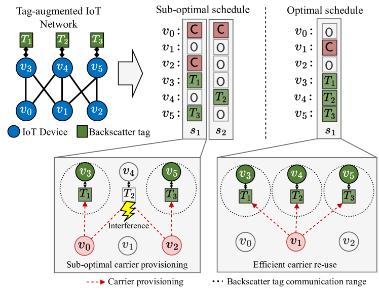
Figure 3. Optimal schedules favor maximum carrier re-use. Example of a tag-augmented IoT network and two possible schedules: the optimal schedule that maximizes carrier re-use while minimizing schedule length, and a sub-optimal schedule.

In tag-augmented scenarios, IoT devices invest considerable resources to support the tags, despite the fact that they may be battery-powered or otherwise resource-constrained. To minimize the resources allocated to supporting the tags, one must devise an efficient communication schedule for tag interrogations (Pérez-Penichet et al., 2020, 2020). A single tag interrogation corresponds to a request-response cycle between an IoT device and one of its hosted battery-free sensor tags, while exactly one of its neighboring IoT nodes provides an unmodulated carrier. More than one unmodulated carrier impinging on any tag causes interference and prevents proper interrogation. Provided that collisions are avoided, scheduling multiple tag interrogations concurrently reduces the schedule’s length, improving latency and throughput in the network (see Figure 3). Furthermore, scheduling one unmodulated carrier to serve multiple tags simultaneously greatly reduces the required energy and spectrum occupancy.

Computing the optimal schedule—minimizing the number of times nodes must generate carriers and minimizing the duration of the schedule—is an NP-hard combinatorial optimization problem (Pérez-Penichet et al., 2020). At first glance, tag scheduling is similar to classic wireless link scheduling in that collisions among data transmissions must be avoided by considering the network topology. Carrier scheduling differs, however, in that we must additionally select appropriate carrier generators while avoiding collisions caused by them upon their neighbors. Simultaneously, we must also minimize resource utilization. The only known scalable solution is a carefully crafted heuristic, which nevertheless suffers from suboptimal performance (Pérez-Penichet et al., 2020). This results in wasted energy and spectral resources, particularly as network sizes grow. We refer to this heuristic as the TagAlong scheduler (Pérez-Penichet et al., 2020) hereafter. Alternatively, one can compute optimal solutions using a constraint optimization solver. We will refer to this scheduler as the optimal scheduler. This scheduler, however, takes a prohibitively long time as network sizes grow, which limits the capacity to adapt to network topology changes. E.g., computing schedules for 10 nodes and 14 tags can take up to a few hours.

In this paper, we leverage Deep Learning (DL) methods to overcome both the scalability limitations of the optimal scheduler and the performance shortcomings of the TagAlong scheduler. However, the DL approach presents its own set of challenges. First, traditional DL methods that have succeeded on problems with fixed structure and input/output sizes (e.g., images and tabular data) are not applicable to the carrier scheduling problem since the latter operates on an irregular network structure, the size of which depends on the number of IoT devices and sensor tags. Second, any given IoT network configuration may have many equivalent optimal solutions, which can confuse Machine Learning (ML) models during training. This is due to symmetries inherent to the carrier scheduling problem, e.g., the schedules are invariant to timeslot permutations when not imposing a fix priority on tag interrogation.

Approach. In this work, we present Deep Graph Attention-based Network Time Tables (DeepGANTT), a new scheduler that builds upon the most recent advances in DL to efficiently schedule the communications of battery-free tags and the supporting carrier generation in a heterogeneous network of IoT devices interoperating with battery-free tags. Upon request from the wireless network, DeepGANTT receives as input the network topology represented as a graph, and generates a corresponding interrogation schedule (Figure 1). The graph representation of the network assumes there is a link between two IoT nodes iff there is a sufficient signal strength between them for providing unmodulated carrier.

DeepGANTT iteratively performs one-shot node classification of the network’s IoT devices to determine the role each of them will play within every schedule timeslot: either remain off ($\mathtt{O}$), interrogate one of its tags ($\mathtt{T}$), or generate a carrier ($\mathtt{C}$), while also avoiding collisions in the network. The objective of the carrier scheduling problem is to reduce the resources needed to interrogate every tag in the network. By minimizing the number of carrier generation slots ($\mathtt{C}$) in the schedule, we reduce energy and spectrum occupancy. As a secondary objective, minimizing the number of required timeslots improves latency and throughput.

We adopt a supervised learning approach based on Graph Neural Networks instead of other paradigms such as reinforcement learning. This choice is mainly motivated by three facts. First, we can leverage the optimal scheduler to generate the training data necessary for a supervised approach. Second, GNNs are particularly successful in handling irregularly structured, variable-size input data such as network topology graphs (Scarselli et al., 2009; Gilmer et al., 2017; Kipf and Welling, 2017). GNNs provide a natural way of capturing the interdependence among neighboring nodes across multiple hops, crucial to avoid collisions. Third, it is straightforward to cast the scheduling problem as a classification task, which is generally tackled with a supervised approach (Bishop and Nasrabadi, 2006; Murphy, 2012).

To train DeepGANTT, we generate random network topologies that are small enough for the optimal scheduler to handle. To avoid the pitfalls of training with multiple optimal solutions per instance, we add symmetry-breaking constraints to the optimal scheduler. Such constraints alter neither the true constraints, nor the objective of the problem. Instead, they narrow the choices of the solver from potentially many equivalent optimal solutions down to a single consistent one. For example, in tag scheduling, the order in which tags are interrogated is irrelevant. Nevertheless, by adopting a specific order (e.g., decreasing order of tag ID) we reduce the number of solutions from the factorial of the number of tags to one.

Contributions. We make the following specific contributions:

• We present DeepGANTT, the first fast and scalable DL scheduler that leverages GNNs to obtain near-optimal solutions to the carrier scheduling problem.

• We employ symmetry-breaking constraints to limit the solution space of the carrier scheduling problem when generating the training data.

• DeepGANTT performs within $3\%$ of the optimum in trained network sizes and scales to $6\times$ larger networks while reducing carrier generation slots by up to $50\%$ compared to the state-of-the-art heuristic. This directly translates to energy and spectrum savings.

• We use DeepGANTT to compute schedules for a real network topology of IoT devices. Compared to the heuristic, our scheduler reduces the energy per tag interrogation by $13\%$ in average and up to $50\%$ for large tag deployments.

• DeepGANTT’s inference time is polynomial on the input size, achieving on average $429\text{\,}\mathrm{ms}\text{/}$ and always below $1.5\text{\,}\mathrm{s}\text{/}$; a radical improvement over the optimal scheduler.

Hence, we show that our scheduler can compute more resource-efficient schedules than the TagAlong scheduler, and that these are almost as good as those of the optimal scheduler (see Figure 2). Moreover, DeepGANTT can generate schedules for considerably larger backscatter networks while still reducing the energy consumption and spectrum occupancy compared to the heuristic. Our scheduler also breaks the scalability limitations of the optimal scheduler, facilitating timely reactions to changes in topology and radio propagation conditions.

The rest of the paper is organized as follows. Sec. 2 gives background information that is useful to understand the paper. Sec. 3 formally describes the carrier scheduling problem. Sec. 4 details the design of DeepGANTT, while Sec. 5 discusses the implementation and training of the model. In Sec. 6, we evaluate DeepGANTT’s performance against previous alternatives and prove that it can also compute schedules for a real IoT network. Lastly, we discuss related work in Sec. 7 and conclude our work in Sec. 8.

2. background

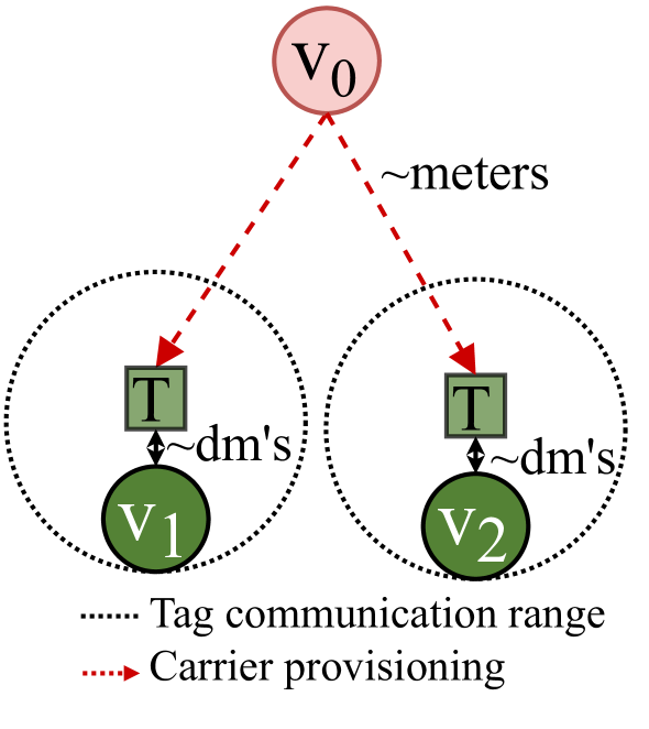
(a) Carrier re-use enabled by tags’ short communication range.

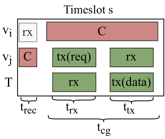
(b) Tag uplink and downlink communication within a timeslot $s$.

Figure 4. The duration of a timeslot is sufficient for an IoT device to interrogate one tag by transmitting a request directed to the desired tag and receiving the response. Furthermore, we leverage the short tag communication range to use a carrier providing node to perform multiple tag interrogations across nodes in the network.

This section gives a quick overview of backscatter communications and the concept of tag-augmented IoT networks, with an intuitive introduction to GNNs.

2.1. Backscatter Communications

Backscatter communication devices are highly attractive because their characteristic low power consumption enables them to operate without batteries. Instead, they can sustain themselves by collecting energy from their environment using energy harvesting modalities. These kinds of devices achieve their low power consumption by offloading some of the most energy-intensive functions, such as the local oscillator, to an external device that provides an unmodulated carrier. Recent works have extended this principle to enable battery-free tags capable of direct two-way communications with unmodified COTS wireless devices using standard protocols such as IEEE 802.15.4/ZigBee or Bluetooth, when supported by an external carrier (Kellogg et al., 2016; Ensworth and Reynolds, 2015; Kellogg et al., 2014; Talla et al., 2017; Iyer et al., 2016; Pérez-Penichet et al., 2016, 2020).

Previous works have demonstrated systems that apply these battery-free communication techniques to augment an existing network of COTS wireless devices with battery-free tags (Pérez-Penichet et al., 2016, 2020, 2020). We refer to this architecture as a tag-augmented IoT network. It enables placing sensors in hard-to-reach locations without having to worry about wired energy availability or battery maintenance. Existing studies have shown how the IoT nodes invest energy to provide carrier support in proportion to the number of carrier slots ($\mathtt{C}$) scheduled and that tags add latency proportionally to the duration of the tag interrogation schedule (Pérez-Penichet et al., 2020). As a consequence, it is critical that we optimize the way unmodulated carrier support is provided (see Figure 3). For this reason, in this work, we focus on the efficiency of the scheduler, given that it bears total influence on resource expenditure.

We adopt a model where each tag is associated with (or hosted by) one IoT device responsible for interrogating it to collect sensor readings. Every IoT node in the network may host zero or more tags. The IoT devices in the network are equipped with radio transceivers that support standard physical layer protocols such as IEEE 802.15.4/ZigBee or Bluetooth. They are able to provide an unmodulated carrier (by using their radio test mode (Pérez-Penichet et al., 2016)) and employ a time-slotted medium access mechanism. The use of a time-slotted access mechanism is motivated by its widespread use in commodity devices and its ease of integration for the battery-free tags. The duration of a timeslot is sufficient for an IoT device to interrogate one tag by transmitting a request directed to the desired tag and receiving the response. Figure 4(b) shows a tag interrogation procedure. First, the carrier providing node $\text{v}_{i}$ listens for a period $t_{req}$ for a request from the interrogating node $\text{v}_{j}$ at its assigned timeslot in the schedule. Upon the request arrival, $\textbf{v}_{i}$ provides a carrier for the duration $t_{cg}$. The interrogating node $\text{v}_{j}$ transmits its request to one of its hosted tags $T$, after which the tag transmits its response back to $\text{v}_{j}$.

When a node interrogates a tag, one of its neighboring IoT nodes must provide an unmodulated carrier (Pérez-Penichet et al., 2020, 2020). Note that both IEEE 802.15.4 and Bluetooth specify a time-slotted access mechanism with the necessary characteristics in their respective standards (IEEE, 2016; Bluetooth SIG, 2021). As shown in Figure 4(a), the short communication range of the tags enables re-using an unmodulated carrier to perform multiple concurrent tag interrogations. However, an IoT node can only interrogate one of its hosted tags per timeslot. When not querying the backscatter tags, the network of IoT nodes performs its own tasks according to its regular schedule. Finally, at least one of the IoT devices is connected to a cloud or edge server where the interrogation schedule can be computed.

The network of IoT nodes keeps track of link state information to determine the connectivity graph among themselves. This information can be relayed periodically or on demand to the cloud or edge server, where it is, together with the tag-to-host mapping, used to assemble the graph representation of the network. Our scheduler uses this graph representation to produce a schedule, as depicted in Figure 1. An interrogation schedule consists of one or more scheduling timeslots, each assigning one of three roles to every IoT device in the network: provide an unmodulated carrier ($\mathtt{C}$), interrogate one of its hosted sensor tags ($\mathtt{T}$), or remain idle ($\mathtt{O}$).

2.2. Graph Neural Networks

GNNs have emerged as a flexible means to tackle various inference tasks on graphs, such as node classification (Scarselli et al., 2009; Hamilton, 2020; Wu et al., 2021). Intuitively, stacking $K$ GNN layers corresponds to generating node embedding vectors taking into account its $K$-hop neighborhood by leveraging the structure of the graph and inter-node dependencies (Gilmer et al., 2017; Kipf and Welling, 2017). These embeddings are typically further processed with linear layers to produce the final output according to the task of interest. E.g., one might perform node classification by passing each node embedding vector through a classification layer. Formally, given a graph $G=\langle V,E\rangle$ defined by the sets of nodes $v\in V$ and edges $(v,u)\in E$, at GNN layer $i$ each node feature vector $h_{v}$ is updated as:

(1) $$h^{(i)}_{v}=f_{1}\left(\,\,h^{(i-1)}_{v},\,\,\underset{u\in\mathcal{N}(v)}{\operatornamewithlimits{AGG\ }}\left[f_{2}\left(h_{u}^{(i-1)}\right)\right]\,\,\right)\,\text{,}$$

where $\mathcal{N}(v)$ is the set of neighboring node feature vectors of node $v$, AGG is a commutative aggregation function, and $f_{1},f_{2}$ are non-linear transformations (Gilmer et al., 2017). Among the main advantages of using GNNs over traditional DL methods are their capability to exploit the structural dependencies of the graph. Furthermore, they are an inductive reasoning method, i.e., GNNs can be deployed to perform inference on graphs other than those seen during training without the need to re-train the model (Hamilton et al., 2017; Veličković et al., 2018; Vesselinova et al., 2020).

3. Problem Formulation

This section formally describes the carrier scheduling problem, i.e., efficiently scheduling the communications of sensor tags and the supporting carrier generation in a network of IoT wireless devices interoperating with battery-free tags. We hereon refer to the IoT devices and to the sensor tags in the network simply as nodes and tags, respectively. We model the wireless IoT network as an undirected connected graph $G$, defined by the tuple $G=\langle V_{a},E\rangle$, where $V_{a}$ is the set of $N$ nodes in the network $V_{a}=\{v_{i}\}_{i=0}^{N-1}$, and $E$ is the set of edges between the nodes $E=\{\langle u,v\rangle|u,v\in V_{a}\}$.

The connectivity among nodes in the graph (edges set $E$) is determined by the link state information collected as described in Section 2.1, i.e., there is an edge between two nodes if and only if there is a sufficiently strong wireless signal for providing the unmodulated carrier (Pérez-Penichet et al., 2020, 2020). We denote the set of $T$ tags in the network as $N_{t}=\{t_{i}\}_{i=0}^{T-1}$, and their respective tag-to-host assignment as $H_{t}:t\in N_{t}\mapsto v\in V_{a}$. A node can host zero or more tags. The role of a node $v$ within a timeslot $s$ is indicated by the map $R_{v,s}:v\!\in\!V_{a},s\!\in\![1,L]\mapsto\{\mathtt{C},\mathtt{T},\mathtt{O}\}$, where $L$ is the schedule length in timeslots. Hence, a timeslot $s_{j}$ consists of an $N$-dimensional vector containing the roles assigned to every node during timeslot $j$: $s_{j}=\left[R_{v_{i},j}|v_{i}\in V_{a}\right]^{\top}$. A timeslot duration is long enough to complete one interrogation request-response cycle between a node and a tag (see Figure 4(b)).

For a given problem instance (wireless network configuration) defined by the tuple $g=\langle G,N_{t},H_{t}\rangle$, the Combinatorial Optimization Problem (COP) of interrogating all sensor values in the network once using the lowest number of carrier generators and timeslots is formulated as follows:

(2) $$\min\,\, \,\,\left(T\times C+L\right)$$

(3) s.t. $$\,\,\forall t\!\in\!N_{t}\,\,\exists!\,\,s\!\in\![1,L]:\,R_{H_{t},s}=\mathtt{T}$$

(4) $$\,\,\forall s\!\in\![1,L]\,\,\forall t\!\in\!N_{t}\,|\,R_{H_{t},s}=\mathtt{T}$$

$$\,\,\;\;\;\;\;\;\;\;\;\;\;\exists!\,v_{j}\!\in\!V_{a}:\,R_{v_{j},s}=\mathtt{C}\wedge(H_{t},v_{j})\in E\,\,\text{,}$$

where $C$ is the total number of carriers required in the schedule, i.e., $C=\left|\{R_{v_{j},s}=\mathtt{C}:v_{j}\!\in\!V_{a},s\!\in\![1,L]\}\right|$. Constraints (3) and (4) enforce that tags are interrogated only once in the schedule and that there is only one carrier-providing neighbor per tag in each timeslot (to prevent collisions), respectively. The objective function (2) is designed to prioritize reducing the number of carrier slots ($C$) over the duration of the schedule ($L$). This is because we are most concerned with energy and spectrum efficiency and because a reduction of $C$ often implies a reduction of $L$, but the converse is not necessarily true. For example, in Figure 1, $v_{2}$ provides a carrier to interrogate $T_{1}$ and $T_{3}$, reducing $C$ and $L$ simultaneously. However, another alternative would be to provide carriers to $T_{1}$ and $T_{3}$ from $v_{1}$ and $v_{2}$ respectively; which would reduce $L$ but not $C$.

4. DeepGANTT: System Design

In this section, we first introduce the design considerations for DeepGANTT to cope with the wireless network requirements and the challenges in carrier scheduling. We then introduce DeepGANTT’s system architecture.

4.1. Design Considerations

DeepGANTT is deployed at an edge or cloud server, where schedules are computed on demand for the IoT network. At least one of the IoT nodes in the network is assumed to be connected to the Edge/Cloud server, and it is responsible for building the IoT network topology graph, emitting the request to the scheduler in the Edge/Cloud, and disseminate the computed schedule to the other devices. The DeepGANTT scheduler receives as input the IoTs network configuration as the tuple $g=\langle G,N_{t},H_{t}\rangle$, i.e., the wireless network topology $G$ and the set of tags $N_{t}$ in the network with their respective tag-to-host assignment $H_{t}$. The scheduler then generates the interrogation schedule $S$ and delivers it to the IoT network. The scheduler may receive subsequent schedule requests by the IoT network either upon addition/removal of nodes or tags, or upon connectivity changes among the IoT devices. Thus, DeepGANTT must be able to react fast to structural and connectivity changes in the wireless network.

From ML ML perspective, every possible configuration of $g$ yields a different graph representation with different connectivity and potentially different input size. Likewise, the output (schedule $S$) may vary in size in terms of both the number of timeslots $L$ and the number of nodes $N$ in the topology (since $s_{j}\!\in\!\mathbb{R}^{N}\forall j\in\{0,\dots L\}$). Moreover, at every timeslot $s_{j}$, every node is assigned to one of three possible actions $\{\mathtt{C},\mathtt{T},\mathtt{O}\}$ (see Section 2.1) based on its neighborhood. We use a GNN-based learning approach to allow DeepGANTT to process variable-sized inputs (network topology) and output (interrogation schedule) sequences while learning the local dependencies of a node in the network (see Sec. 2.2).

For carrier scheduling, exploiting the structural dependencies of the nodes’ $K$-hop neighborhood allows to efficiently schedule carriers while avoiding interference. Moreover, since GNNs are an inductive reasoning ML method, we can deploy the model without the need to re-train it for different network configurations in terms of the number of IoT nodes $N$, their connectivity, and the number of sensor tags $T$.

4.2. System Architecture

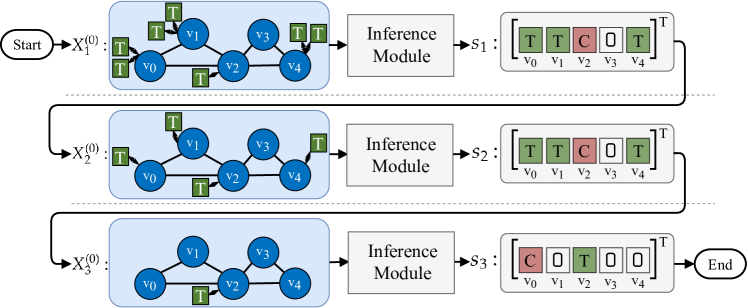
(a) DeepGANTT iteratively performs one-shot node classification, one timeslot at a time, removing scheduled tags from the topology and repeating the process until no more tags remain.

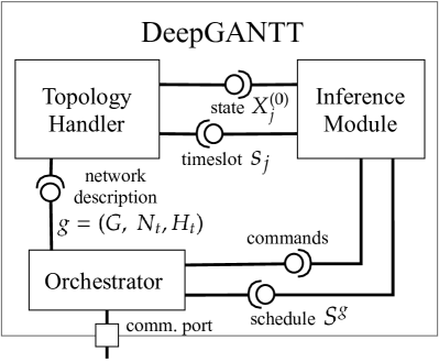
(b) The three core components of DeepGANTT interact among themselves and with the exterior to generate schedules.

Figure 5. DeepGANTT’s system architecture and the Inference Module’s procedure to generate schedules.

We model the carrier scheduling problem as an iterative one-shot node classification problem. The inner workings of DeepGANTT are illustrated in Figure 5(a): on each iteration $j$, DeepGANTT’s inference module assigns each node in the topology to one of three classes corresponding to the possible node actions: $\{\mathtt{C},\mathtt{T},\mathtt{O}\}$. Hence, each iteration $j$ generates a timeslot $s_{j}$. Each predicted timeslot is checked for compliance with the constraints in Eq. 3 and  4. After each iteration, the topology’s node feature vector is updated by removing one tag from the nodes that were assigned class $\mathtt{T}$ (interrogate). This process is repeated until all tags have been removed from the cached network configuration.

The DeepGANTT scheduler consists of three submodules, as depicted in Figure 5(b). The Orchestrator is DeepGANTT’s coordinating unit and interacts with the outside world through its communication port. It is responsible for providing the problem description to the Topology Handler and interfacing with the Inference Module. The Topology Handler maintains the problem description, provides it to the Inference Module in a format suitable for the ML model, and updates its state according to the predicted timeslots.

Since the Inference Module is trained on the basis of a stochastic process, the Topology Handler includes a fail-safe functionality to make sure that the predictions comply with the constraints in Eqs. (3) and (4). In case of failure, the Topology Handler restores compliance by randomly shuffling tag and node IDs and retrying. This does not alter the final schedules.

4.3. Input Node Features

At timeslot $j$, the Inference Module receives as input a node feature matrix $X^{(0)}_{j}\in\!\mathbb{R}^{N\times D}$ containing the row-ordered node feature vectors $x_{i,j}^{(0)}\in\mathbb{R}^{D},\forall i\in V_{a}$, where $D$ represents the number of features representing a node’s input state. Since the tags lie in the immediate proximity of a node, and each of them interacts only with their host, we model them as a feature in their host’s input feature vector. One can also include additional features to assist the GNN during inference. Hence, we consider three different node features:

• Hosted-Tags: the number of tags hosted by a node.

• Node-ID: integer identifying a node in the graph.

• Min. Tag-ID: the minimum tag ID among tags hosted by a node. Since a node can host several tags, the min. Tag-ID represents only the lowest ID value among its hosted tags.

Intuitively, the number of tags hosted by a node is decisive for assigning carrier-generating nodes. E.g., if one node hosts all tags, this node should never be expected to provide the unmodulated carrier in the schedule. Similarly, the node hosting the greatest number of tags is unlikely to be a carrier provider in the schedule. For this reason, Hosted-Tags is always included as an input node feature. Moreover, including the node-ID and the minimum tag-ID can provide the scheduler with context on how to prioritize carrier-provider nodes, and with an order to interrogate the tags.

4.4. Inference Module

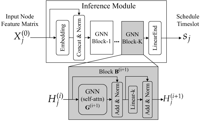
Figure 6. At the core of the inference module there are $K$ GNN layers with self-attention. The Inference Module implements DeepGANTT’s ML model.

The Inference Module is the central learning component of DeepGANTT and contains the ML model for performing inference. In the following, we describe in detail the Inference Module’s ML architectural components. The Inference Module consists of three parts, as depicted in Figure 6.

Embedding. The input node feature matrix $X^{(0)}_{j}$ is first transformed by an Embedding component with the aim to assist the subsequent message-passing operations in performing better injective neighborhood aggregation. That is, enabling each node to better distinguish its neighbors. The embedding transformation of $X^{(0)}_{j}$ is described by:

(5) $$H^{(0)}_{j}=\text{LN}\left(\bigparallel\left[X^{(0)}_{j},\text{FNN}_{e}\left(X^{(0)}_{j}\right)\right]\right)\,\text{,}$$

where LN corresponds to the layer normalization operation from Ba et al. (Ba et al., 2016), and $\bigparallel$ represents the concatenation operation. $\text{FNN}_{e}$ corresponds to a fully-connected neural network layer (FCNN) with a non-linear transformation as:

(6) $$\text{FNN}_{e}(X^{(0)}_{j}) \,=\, \text{LeLU}\left(\text{FCNN}_{e}(X^{(0)}_{j})\right)$$

(7) $$\text{FCNN}_{e}(X^{(0)}_{j}) \,=\, X^{(0)}_{j}W_{e}+b_{e}\,\,\text{,}$$

with the leaky ReLU operator LeLU and NN parameters $W_{e}\in\mathbb{R}^{D\times D_{e}},b_{e}\in\mathbb{R}^{D_{e}}$. The embedding outputs the node feature matrix $H^{(0)}_{j}\in\mathbb{R}^{N\times(D+D_{e})}$.

Stacked GNN Blocks. The output from the embedding component $H^{(0)}_{j}$ represents the input to a stack of $K$ GNN blocks $\{B^{(i+1)}\}_{i=0}^{K-1}$. The inner structure of each GNN block is depicted in the lower part of Figure 6. We stack $K$ different GNN blocks to allow nodes to receive input from their $K$-hop transformed neighborhood. Moreover, we select summation as the aggregation operation (see Eq. 11) motivated by the results of Hamilton et al. (Hamilton et al., 2017). Each GNN block $B^{(i+1)}$ receives as input the previous layer output $H^{(i)}_{j}$ and performs the following operations:

(8) $$H^{(i+1)}_{j} \,=\, \textbf{B}^{(i+1)}(H^{(i)}_{j})$$

(9) $$\textbf{B}^{(i+1)}(H^{(i)}_{j}) \,=\, \text{LN}\left(\tilde{H}^{(i+1)}_{j}+\text{FNN}_{B}^{(i+1)}\left(\tilde{H}^{(i+1)}_{j}\right)\right)$$

(10) $$\tilde{H}^{(i+1)}_{j} \,=\, \text{LN}\left(H^{(i)}_{j}+\textbf{G}^{(i+1)}(H^{(i)}_{j})\right)\,\text{.}$$

Eq. 10 corresponds to a multi-head self-attention GNN activation $\textbf{G}^{(i+1)}$ followed by an Addition&Normalization component in Figure 6. Subsequently, Eq. 10 implements a per-node FCNN with a non-linear transformation, followed by another Add&Norm component. Analogous to Eq. 7, each block’s per-node $\text{FNN}_{B}^{(i+1)}$ has parameters $W_{b}^{(i+1)}$ and $b_{b}^{(i+1)}$ followed by a leaky-ReLU.

The operation $\textbf{G}^{(i+1)}$ in Eq. 10 implements a scaled dot-product multi-head self-attention GNN (Vaswani et al., 2017; Shi et al., 2021). Each of the $N$ row-ordered node feature vectors $H^{(i)}_{j}=\{h_{j,t}^{(i)}\}_{t=0}^{N-1}$ is updated at GNN layer $\textbf{G}^{(i+1)}$ by the following message-passing operation (for simplicity, we omit the timeslot subscript $j$):

(11) $$h_{t}^{(i+1)} = \text{FCNN}_{upt}^{(i+1)}\!\!\left(h_{t}^{(i)}\right)+\bigparallel_{m=1}^{M}\left[\sum_{p\in\mathcal{N}(t)}\alpha^{(i+1)}_{m,tp}\tilde{v}_{m,p}^{(i+1)}\right]$$

(12) $$\tilde{v}_{m,t}^{(i+1)} = \text{FCNN}_{m,val}^{(i+1)}\left(h_{t}^{(i)}\right)$$

(13) $$\alpha^{(i+1)}_{m,tp} = \frac{\Gamma\left(q_{m,t}^{(i+1)},k_{m,p}^{(i+1)}\right)}{\sum\limits_{u\in\mathcal{N}(t)}\Gamma\left(q_{m,t}^{(i+1)},k_{m,u}^{(i+1)}\right)}$$

(14) $$q_{m,t}^{(i+1)} = \text{FCNN}_{m,qry}^{(i+1)}\!\left(h_{t}^{(i)}\right)$$

(15) $$k_{m,t}^{(i+1)} = \text{FCNN}_{m,key}^{(i+1)}\!\left(h_{t}^{(i)}\right)$$

(16) $$\Gamma\left(A,B\right) = \,\,\frac{\exp\left(A^{\top}B\right)}{\sqrt{d}}\,\text{,}\,\,A,B\in\mathbb{R}^{d}\,\,\,\text{.}$$

Eq. 11 is the main node update operation for each node, consisting of adding two parts. First, a transformation of the target node’s feature vector through $\text{FCNN}_{upt}^{(i+1)}$. Second, the concatenated $M$-heads of the attention operations with the target node’s neighbors. Each self-attention operation $m$ consists of a weighted sum over transformed neighboring node feature vectors $\tilde{v}_{m,t}^{(i+1)}$, inspired by the attention operations by Vaswani et al. (Vaswani et al., 2017). Each of the neighbors’ node feature vectors are transformed by the layer $\text{FCNN}_{m,val}^{(i+1)}$ in Eq. 12. The weights $\alpha^{(i+1)}_{m,tp}$ at attention head $m$ from neighbor source $p$ to target update node $t$ are obtained through Eq. 13 over the scaled dot product operation $\Gamma$ (Eq. 16) between query $q_{m,t}^{(i+1)}$ and key $k_{m,t}^{(i+1)}$ transformations of the target node (see Eq. 14) and the source neighbor node (see Eq. 15), respectively.

There are multiple reasons motivating the use of attention. First, it allows to leverage neighboring nodes’ contributions differently. Second, attention has provided better results for node classification tasks (Veličković et al., 2018) compared to isotropic GNNs (Kipf and Welling, 2017; Hamilton et al., 2017). Moreover, conventional GNN node classification benchmarks assume that nodes in a spatial locality of the graph assume similar labels and leverage the fixed-point theorem property in stacking GNNs (Kipf and Welling, 2017). This greatly contrasts with the carrier scheduling problem, in which neighboring nodes are mostly expected to have different classes (a node provides a carrier, neighbors interrogate tags). Finally, attention serves as a counteracting factor for this property when combined with skip-connections: it builds deeper networks that can learn contrasting representations at each layer.

Classification Layer. The output from the $K$ GNN blocks is then fed to a FCNN followed by a Softmax for obtaining a per-node probability distribution over the classes that correspond to the possible node actions $\{\mathtt{C},\mathtt{T},\mathtt{O}\}$. Finally, each node is assigned to the class with the highest probability.

Note that all parameters from the Inference Module listed (Eqs. 5–15) are shared across timeslots $s_{j}$.

5. Learning to Schedule

Table 1. The interrelation between data generation and input node features strongly impact the model’s performance. Including symmetry-breaking constraints dramatically improves the model performance. Interdependence of data generation and input feature configuration for an Inference Module of six GNN-Blocks. $S_{corr}$ indicates percentage of problem instances for which the NN delivers a complete schedule. F1-score is provided for $\mathtt{C}$ (carrier class).

Symmetry breaking:	Disabled			Enabled
Performance Metric [%]:	Accuracy	F1-score	$S_{corr}$	Accuracy	F1-score	$S_{corr}$
Features-1 (Hosted-Tags):	85.69	57.78	27.04	86.61	60.54	10.11
Features-2 (Hosted-Tags + Node-ID + Min. Tag-ID.):	86.40	59.82	47.96	99.22	97.36	99.64

This section explores how the Inference Module’s ability to compute interrogation schedules is influenced by two factors. On one hand, the interdependence between the choice of input node features and on the other the configuration of the training data generation. Additionally, we explore the influence of ML model complexity in terms of the number of GNN blocks on the Inference Module’s performance. This exploratory analysis resulted in selecting an Inference Module composed of 12 GNN blocks.

5.1. Training Data Generation

The carrier scheduling problem, as described in Eqs. 2-4, presents symmetries that result in multiple optimal solutions which confuse the DL model while training. In the following, we describe how we leverage symmetry-breaking constraints in the constraint optimizer to generate a training dataset with unique optimal solutions.

As an example of these symmetries consider that: because the order of the timeslots in the schedule is irrelevant, a schedule of duration $L$ is equivalent to $L!$ other schedules. A similar set of symmetries appears among all tags hosted by the same node as the order of interrogating them is also irrelevant. To make matters worse, a given set of tags can often be served by more than one carrier generator, therefore introducing more symmetries.

Symmetry-Breaking Constraints. To overcome the confusion that these symmetries might cause to a learning-based model during training, we further constrain the carrier scheduling problem in a way that eliminates symmetries but does not otherwise alter the problem. To that end, we enforce lexicographical minimization of a vector of length $T$ that indicates the timeslot where each tag is scheduled. This automatically eliminates symmetries related to the order of tag interrogations. Similarly, we also lexicographically minimize another length-$T$ vector containing the node that provides the carrier for each tag; which eliminates symmetries related to multiple potential carrier nodes.

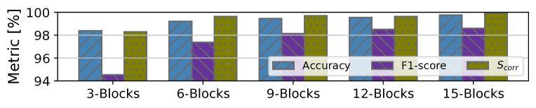
Figure 7. Increasing the number of GNN-Blocks improves the performance of the NN model. The NN reaches a saturation point for the F1-score at approx. 12 layers.

5.2. ML Model Validation Setup

We implement all components in the Inference Module using PyTorch (Paszke et al., 2019). For the GNNs layers $\textbf{G}^{(i+1)}$, we use the PyG self-attention based GNN TransformerConv implementation (Fey and Lenssen, 2019).

Input Features. We consider two different feature configurations for the input node feature matrix $X_{1}^{(0)}\in\mathbb{R}^{N\times D}$: Features-1 includes only the Hosted-Tags ($D=1$), and Features-2 considers Features-1 plus the Node-ID and minimum Tag-ID among the tags hosted by a node ($D=3$).

Validation Dataset. We generate small-sized problem instances of varying sizes and number of tags from two to ten nodes ($N\in[2,10]$), and hosting one to 14 tags ($T\in[1,14]$). We generate these graphs using the random geometric graph generator from NetworkX (Hagberg et al., 2008) to guarantee that these graphs can exist in 3D space. As the network size varies, we make sure to maintain a constant network spatial density. We uniformly assign tags to hosts at random. We employ a constraint optimizer to compute solutions for a total of 520000 problem instances both including and without including the symmetry-breaking constraints. As constraint optimizers, we employ MiniZinc (Nethercote et al., 2007) and OR-Tools (Perron and Furnon, 2019). The problem instances are divided into a train-set and a validation-set using a 80%-20% split. Since we perform a per-node classification for every scheduling timeslot (see Figure 5(a)), we further consider each timeslot input-target pair $(X_{j}^{(0)},s_{j})$ as a training sample, which yields an approximate total of 1.5 million samples.

Validation Metrics. We consider both ML metrics and an application related metric to evaluate a model’s performance. From the ML perspective, we employ overall accuracy, and the carrier class ($\mathtt{C}$) F1-score due to its crucial role in avoiding signal interference for tag interrogation. For the application-related metric we consider the percentage of correctly computed schedules $S_{corr}$. This metric indicates the percentage of problem instances for which the already-trained ML model produces a complete (all timeslots) and correct (fulfilling carrier scheduling constraints) schedule. At inference time, the Topology Handler handles these unlikely cases as described in Section 4.2.

5.3. ML Model Training

We train the Inference Module with the Adam optimizer (Kingma and Lei Ba, 2015) on the basis of mini-batch gradient descent with standard optimizer parameters and an initial learning rate of $10^{-3}$. The ML model should give greater importance to the carrier-generating node class ($\mathtt{C}$) since it can subsequently determine the tags that can be interrogated or not due to signal interference. Hence, we build upon the cross-entropy loss for classification and propose an additional factor to account for greater importance to the carrier class ($\mathtt{C}$):

(17) $$L_{batch} = \frac{1}{N_{b}}\sum_{\hat{y}=0}^{N_{b}-1}L_{x}(\hat{y},y)\,\,L_{1}(\hat{y},y)+\rho||\hat{W}||_{2}^{2}$$

(18) $$L_{x}(\hat{y},y) = -\!\!\!\!\!\sum_{k\in\{\mathtt{C},\mathtt{T/O}\}}\!\!\!y_{k}\log(\hat{y}_{k})$$

(19) $$L_{1}(\hat{y},y) = \exp\left(||(\hat{y}==\mathtt{C})-(y==\mathtt{C})||\right)\,\text{,}$$

where $N_{b}$ is the number of nodes in the mini-batch, $\rho$ is the regularization hyperparameter, and $\hat{W}$ represents the tensor containing all the learning parameters undergoing gradient descent. We implement learning rate decay by $2\%$ every epoch, and early stopping after 25 subsequent epochs without minimization of the test loss, and save the best-performing model on the basis of the F1-score.

5.4. Validation Results

The Inference Module considered for evaluating data generation strategies and node feature representation consists of six GNN-blocks. We empirically chose the number of GNN-blocks for the first experiments based on a trade-off between model training time and performance. After establishing the best combination of input node feature representation and data generation strategy, we analyze the influence in performance of ML model complexity.

5.4.1. Data Generation and Input Features Interdependence

The influence of both input node feature representation and data generation configuration in model performance is depicted in Table 1. Regardless of the data-generating configuration, an enriched node feature representation (including more node features) leads to an increase in accuracy and F1-score. There are two possible reasons for this. First, by increasing the node feature dimension $D$, we ensure that the GNNs can perform more efficient injective neighborhood aggregation (to better distinguish neighboring node contributions). This is realized by making it less likely for two nodes to have the same input feature vector to the GNN. Second, both the Nodes-ID and Tags-ID feature serve as a node’s positional encoding information in a graph, a property that assists the model in breaking graph symmetries (You et al., 2019; Dwivedi et al., 2020).

Additionally, an enriched node feature representation leads to an increase of $S_{corr}$, regardless of the chosen data generation configuration: $20.92\%$ and $89.53\%$ improvement from Features-1 to Features-2 for the standard and the symmetry-breaking configurations, respectively. The constraint optimizer explicitly uses the Node-ID and Tag-ID to compute the optimal solution in the symmetry-breaking configuration, which is why providing the ML model with these features is crucial for it to be able to learn the structural dependencies in the topologies. Implementing symmetry-breaking measurements in the data generation procedure is a critical measure for allowing the NN model to generate complete schedules (highest increase in $S_{corr}$). Since we explore a supervised learning approach, it is crucial to constrain the mapping between inputs and targets for the NN model to learn consistent graph-related structural dependencies.

5.4.2. Influence of the Number of GNN-Blocks

To analyze the influence of the required $K$-hop neighborhood aggregation of the GNN model, we analyze the model’s performance as we vary the number of GNN-Blocks while keeping other architectural components constant to the values found by extensive empirical analysis. Specifically, we set the embedding dimension to $D_{e}=48$, the number of attention heads to $M=2$, and the GNN-Blocks’ hidden feature dimensions to $D_{H}^{(i)}=200$. Figure 7 illustrates how increasing the number of GNN-Blocks increases the performance of the NN model: the F1-score increases to a saturation point around 12 layers. Although the 15-layer model exhibits the highest $S_{corr}$, subsequent experiments showed that this model overfits and hence is unable to scale to larger problem instances.

Inference Module. Based the findings of this section, DeepGANTT’s Inference Module consists of 12 GNN blocks and is trained on $\sim\!\!\!424000$ small-sized problem instances (IoT networks of up to 10 nodes and 14 tags) obtained from the optimal scheduler as described in Section 5.3. We used an NVIDIA Titan RTX for $131$ epochs before reaching the early-stop condition. The model achieved $99.56\%$ accuracy, a carrier-class F1-score of $98.51\%$, and a percentage of correctly computed schedules of $S_{corr}=99.88\%$.

6. Evaluation

After designing DeepGANTT’s Inference Module in Section 5, in this section, we compare DeepGANTT’s results to those of the TagAlong scheduler (Pérez-Penichet et al., 2020) and the optimal scheduler. We highlight the following key findings:

• DeepGANTT performs within 3% of the optimal scheduler on the average number of carriers used, while consistently outperforming TagAlong by up to 50%. This directly translates into energy and spectrum savings for the IoT network.

• Our scheduler scales far beyond the problem sizes where it was trained, while still outperforming TagAlong; therefore enabling large resource savings well beyond the limits of the optimal scheduler.

• We deploy DeepGANTT to compute schedules for a real IoT network of 24 nodes. Compared to the TagAlong scheduler, DeepGANTT reduces the energy per tag interrogation by $13.1\%$ in average and up to $51.6\%$.

• With polynomial time complexity and a maximum observed computation time of $1.49\text{\,}\mathrm{s}\text{/}$, DeepGANTT’s speed is comparable to TagAlong’s, and well within the needs of a practical deployment.

Baselines. To conduct our evaluation, we consider two baselines: i) the optimal scheduler, which corresponds to using a constraint optimizer for computing the optimal solution including the symmetry-breaking constraints for topologies of up to $10$ nodes and $14$ tags, and ii) the TagAlong scheduler, the state-of-the-art heuristic algorithm for computing interrogation schedules for the scope of backscatter IoT networks considered in this work (Pérez-Penichet et al., 2020).

Evaluation Section Structure. This section is structured as follows. Sec. 6.1 benchmarks DeepGANTT’s performance against the optimal scheduler and the TagAlong scheduler for topologies of up to $10$ nodes and $14$ tags previously unseen to DeepGANTT (test set). Sec. 6.2 analyzes DeepGANTT’s gains over TagAlong for topologies well beyond the practical applicability of the optimal scheduler of up to $60$ nodes and $160$ tags (generalization set). Sec. 6.3 then briefly describes DeepGANTT’s time complexity and its computation times. Finally, Sec. 6.4 demonstrates DeepGANTT’s ability to produce schedules for a real IoT network of $N=24$ nodes under different number of tags configurations.

6.1. Test Set Performance

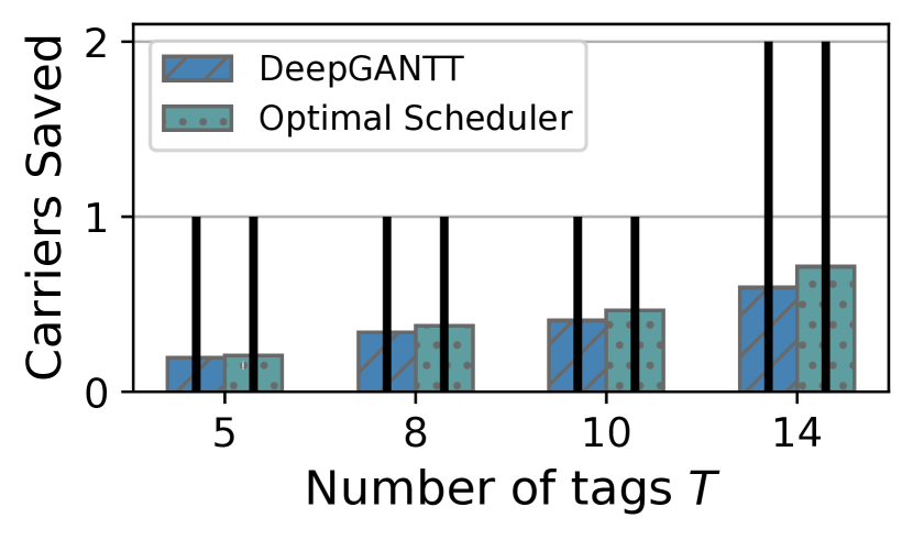
(a) Average number of carriers saved relative to TagAlong.

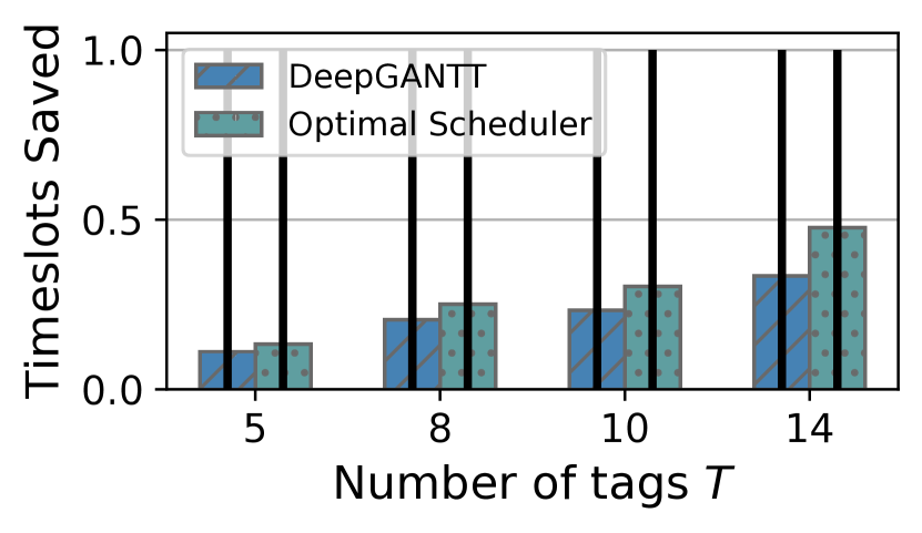
(b) Average timeslot savings relative to TagAlong.

Figure 8. DeepGANTT largely mimics the optimal scheduler both in terms of carriers saved and timeslots saved. Average gain for networks of 10 IoT nodes and various numbers of tags in the test dataset. The black bars depict the 10 and 90 percentiles.

We hereby demonstrate DeepGANTT’s ability to mimic the behaviour of the optimal scheduler to produce interrogation schedules and exhibit similar gains as the optimal scheduler’s performance over the TagAlong heuristic.

Test Dataset. We consider topologies consisting of $\sim\!\!106000$ problem instances of up to $10$ nodes and $14$ tags for which it is still possible to deploy the optimal scheduler.

Test Metrics. We compare the number of carrier slots in the generated schedules since it directly affects the IoT network’s overall energy consumption. Specifically, for every evaluation problem instance we compute DeepGANTT’s saved carriers as $C_{d}-C_{t}$ and, those of the optimal scheduler as $C_{o}-C_{t}$; where $C_{d}$, $C_{t}$, and $C_{o}$ are the number of carriers scheduled by the DeepGANTT, TagAlong and the optimal schedulers respectively. Furthermore, we analyze the total schedule length, since it directly relates to the latency of communications in the wireless network. We compute the timeslots savings in a manner analogous to the carrier savings.

Test Results. Figure 8(a) shows the average number of carriers saved compared to TagAlong (higher is better) for various network sizes in the test dataset. DeepGANTT’s performance is very close to that of the optimal scheduler in all cases. The number of timeslots in the schedule is the secondary objective in the tag scheduling problem; this is because, while the duration of the schedule can impact latency and other performance metrics in the network, the number of carriers directly impacts energy and spectral efficiency. Note that reducing the number of carrier slots, can potentially also shorten the schedule owing to carrier reuse (Pérez-Penichet et al., 2020). As depicted in Figure 8(b), DeepGANTT largely mimics the performance of the optimal scheduler regarding timeslot savings. Our scheduler outperforms the TagAlong scheduler in $98.2\%$ of the test-set instances. On those instances where TagAlong schedules are shorter, it is by one timeslot at most.

6.2. Generalization Performance

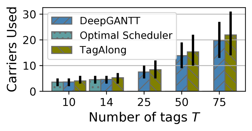
(a) Average number of carriers used for networks of 10 IoT nodes.

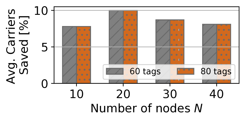
(b) Average percentage of carriers saved compared to TagAlong.

Figure 9. DeepGANTT scales far beyond the range of data where the optimal schedules used in training are available, while outperforming TagAlong by a growing margin (9(a)) The black bars depict the 10 and 90 percentiles. DeepGANTT also maintains an average saving of almost 10% in scheduled carriers while scaling up to four times the maximum training network size (9(b)).

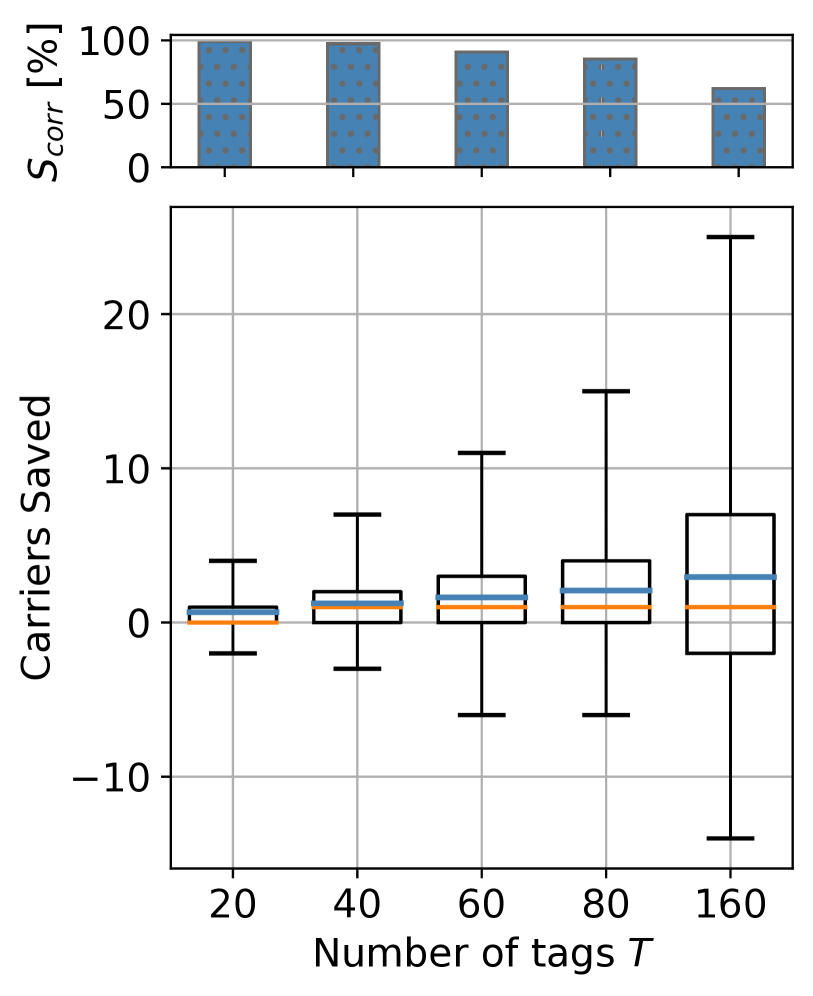
(a) 10 node topologies.

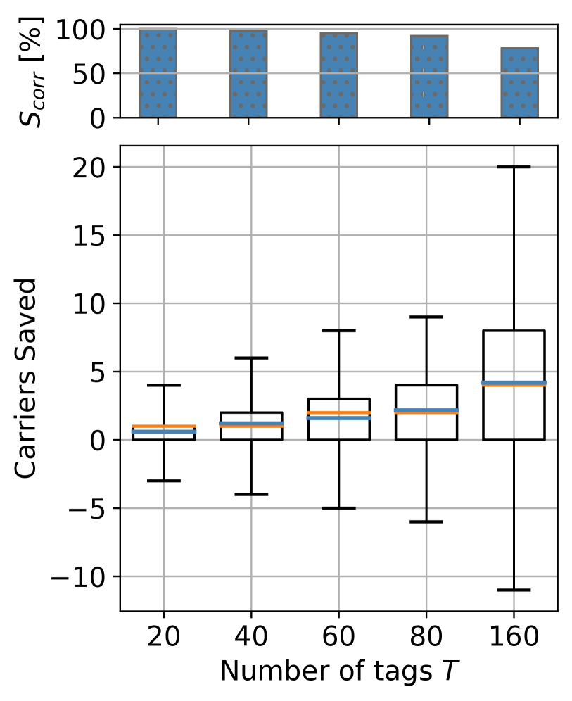
(b) 20-node topologies.

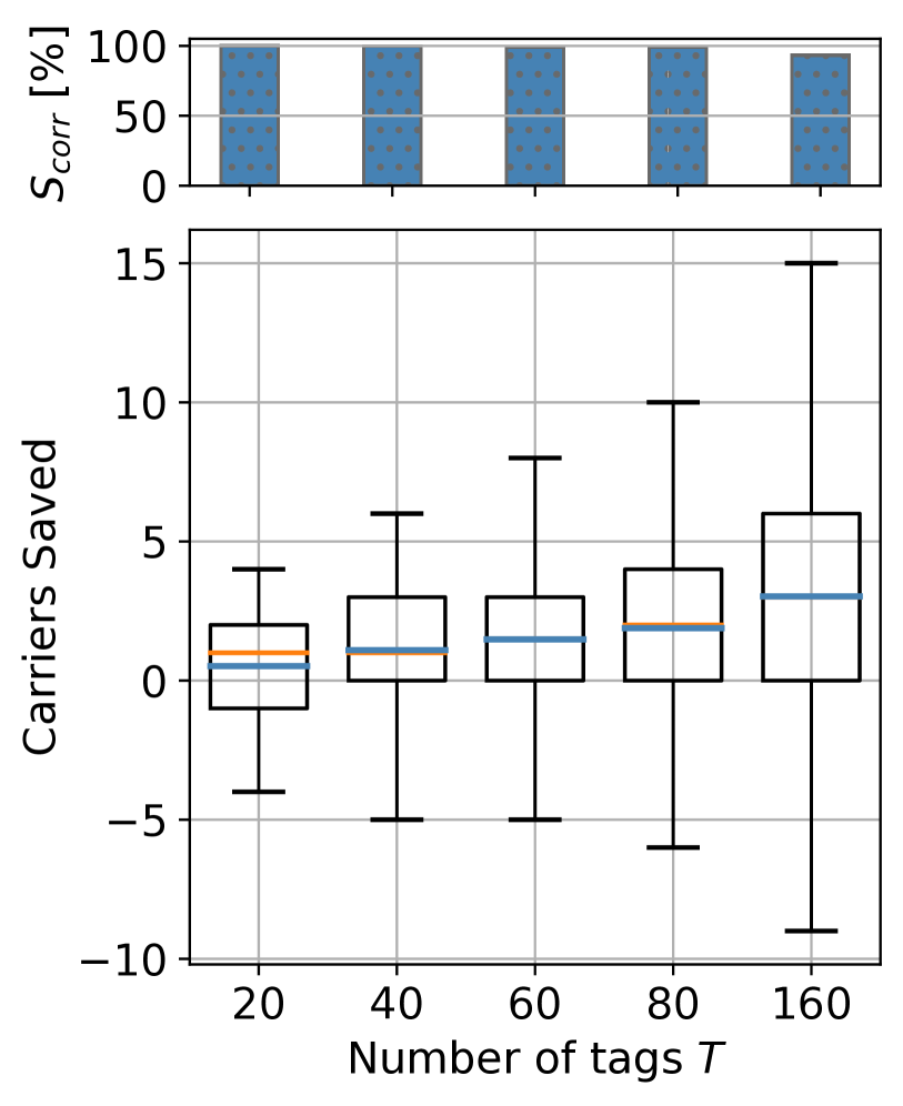
(c) 40-node topologies.

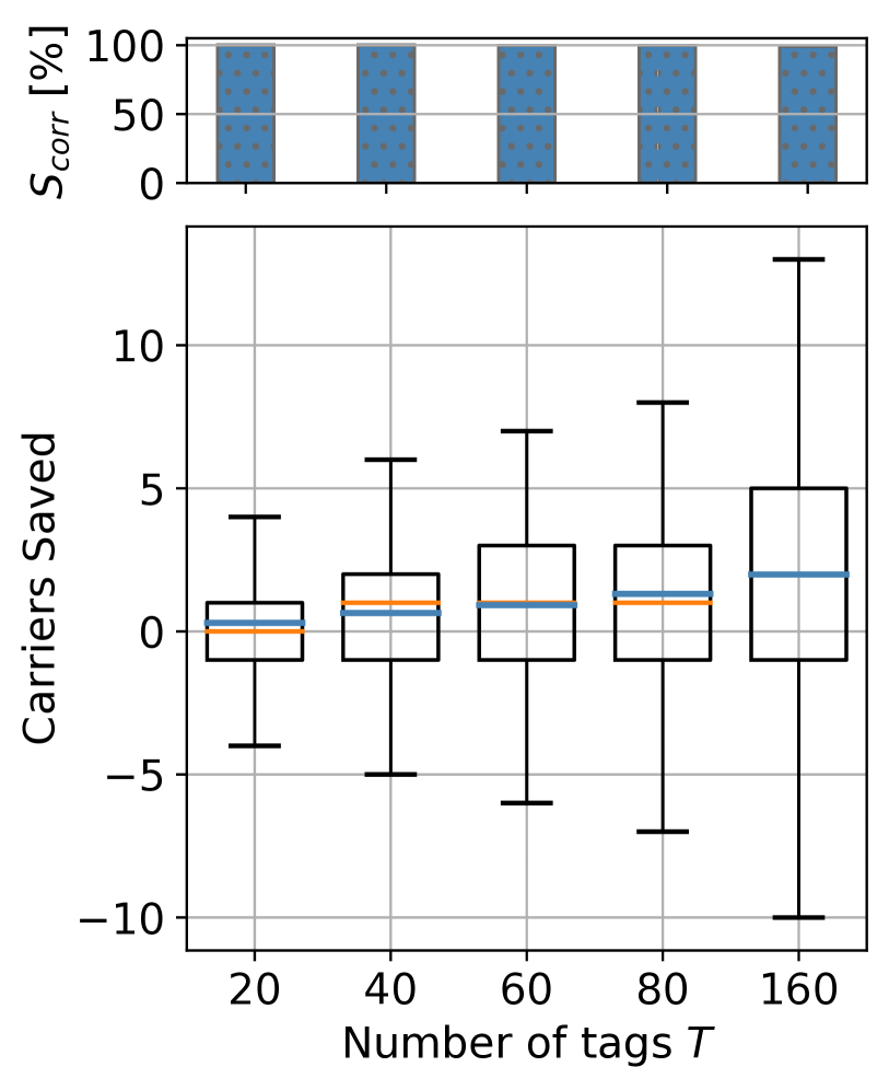
(d) 60-node topologies.

Figure 10. DeepGANTT outperforms TagAlong even when increasing the topology sizes far beyond those seen on training. Scaling capabilities of DeepGANTT when compared to the TagAlong heuristic in terms of carrier savings. The model achieves a maximum carrier reduction of up to $43.42\%$, $43.86\%$, $33.93\%$, $32.14\%$ for 160 tags and $10$, $20$, $40$, and $60$ nodes, respectively. The blue and the orange line represent the mean and the median, respectively. Box extents delimit 25 and 75 percentiles. Whiskers delimit 1 and 99 percentiles. The model also has a high success rate ($S_{corr}$), especially for larger topologies.

We now analyze the capabilities of DeepGANTT in computing schedules for problem sizes well beyond those observed during training and compare its performance against the TagAlong scheduler. The ability to generalize this way directly translates into better scalability than that of the optimal scheduler.

Generalization Dataset. We consider $1000$ problem instances for every $(N,T)$ pairs from the sets $N\in\{10,20,30,40,60\}$ and $T\in\{20,40,60,80,160\}$, i.e., $25000$ different IoT wireless networks.

Metrics. We consider the same metrics as those used in Sec. 6.1.

Generalization Results. Figure 9(a) shows a comparison of the average number of carriers utilized (lower is better) on problem sizes beyond those used in training. DeepGANTT outperforms TagAlong by a growing margin well beyond the maximum size of optimal solutions seen in training (beyond $10$ nodes and $14$ tags). Compared to TagAlong, DeepGANTT is able to reduce the percentage of necessary carriers $\sim\!$7\text{\,}\mathrm{\char 37\relax}\text{/}10\text{\,}\mathrm{\char 37\relax}\text{/}$$ on average for large numbers of tags, as depicted in Figure 9(b).

Figure 10 depicts the number of carriers saved and the percentage of correctly computed schedules $S_{corr}$ for different network size configurations. DeepGANTT consistently increases the mean number of carriers saved as the number of tags increases for all considered configurations. While there are cases where TagAlong outperforms DeepGANTT, these are actually rare occurrences; this is evident by the positive mean and the location of the 25-percentiles. Additionally, DeepGANTT’s percentage of correctly-computed schedules ($S_{corr}$) decreases for the 10-node 80-tags case, but remains above $99\%$ for the 30, 40 and 60 nodes problem instances, for all the number of tags considered. DeepGANTT is able to reduce the number of carriers by up to $50\%$ for all number of nodes configurations in Figure 10.

6.3. Computation Time

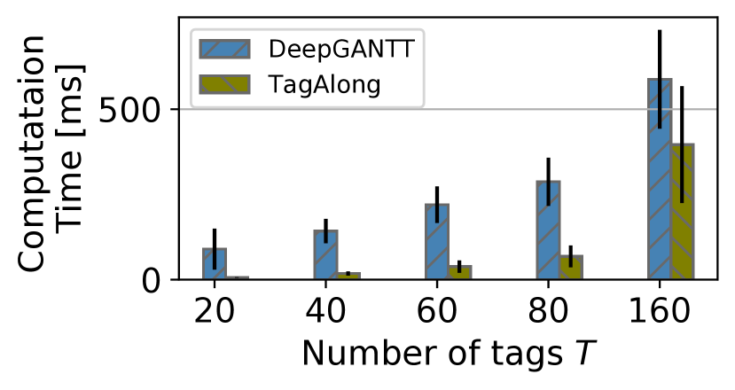
(a) Average runtimes for 10 Nodes.

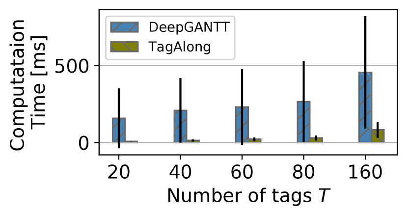
(b) Average runtimes for 60 Nodes.

Figure 11. While TagAlong runs faster than DeepGANTT, both run times are so small that the difference is negligible. Run time comparison of DeepGANTT and TagAlong for 10 and 60 IoT nodes with various numbers of tags. The black bars represent the standard deviation.

A determining factor for the real-world applicability of a scheduler is the computation time. Figure 11 depicts a run time comparison of DeepGANTT and TagAlong on the same hardware. While TagAlong runs faster, the absolute values are so small that the difference is negligible in practice. Note that for the largest problem instances considered ($40$ nodes and $80$ tags), the maximum runtime recorded was $1.49\text{\,}\mathrm{s}\text{/}$, with an average runtime of $0.25\text{\,}\mathrm{s}\text{/}$. This is in stark contrast with the optimal scheduler that takes several hours to compute schedules for just 10 nodes and 14 tags.

Time Complexity. In general, an attention-based message passing operation has time complexity $\mathcal{O}(N\!+\!|E|)$, where $N$ is the number of nodes in the graph and $|E|$ is the number of edges (Veličković et al., 2018). In the worst case, DeepGANTT performs $T$ complete ML model passes, one for every tag in the wireless network. Hence, the complexity of our algorithm is polynomial in the input size: $\mathcal{O}(T(N\!+\!|E|))$.

6.4. Performance on a Real IoT Network

In this section we deploy DeepGANTT to compute tag interrogation schedules for a real IoT network and compare its performance with that of the TagAlong scheduler. We show that DeepGANTT can achieve up to $51.6\%$ energy savings in tag interrogation.

Setup. We use an indoor IoT testbed consisting of 24 Zolertia Firefly devices (see Figure 12(a)). The devices run the Contiki-NG operating system (Oikonomou et al., 2022), communicate using IPv6 over IEEE 802.15.4 Time-Slotted Channel Hopping (TSCH) (Duquennoy et al., 2017), and use RPL as routing protocol (Winter, 2012). We collect the link connectivity among the IoT nodes every 30 min over a period of four days. We assume there is a link between any given pair of nodes if there is a signal strength of at least $-75\text{\,}\mathrm{d}$Bm for carrier provisioning. The IoT network exhibits a dynamic change of node connectivity over the observed period of time (see Figure 12(b)). We augment each of the collected network topologies with randomly assigned tags in the range $T\in\{10,25,50,75,85\}$, $100$ assignments per $T$ value.

Metrics. Apart from the carriers saved metric employed in Sec. 6.1 and 6.2, we also include the average energy per tag interrogation $\tilde{E}$, which is the total energy for tag interrogations $E_{tot}$ divided by the number of tags in the network. Based on Figure 4(b), $\tilde{E}$ is given by:

(20) $$\tilde{E}=\frac{E_{tot}}{T}=P_{tx}t_{tx}\!+\!P_{rx}\left(\frac{C}{T}t_{req}\!+\!t_{rx}\right)\!+\!P_{tx}\left(t_{req}\!+\!\frac{C}{T}t_{cg}\right)\text{,}$$

where $C$ is the number of carriers used in the schedule, $T$ is the number of tags in the network, and both $P_{rx}$ and $P_{rx}$ correspond to the radio power at transmit and receive mode, respectively. We adopt $P_{rx}=72mW$, $P_{tx}=102mW$ based on the Firefly’s reference values. Moreover, we assume $t_{req}=t_{tx}=128\mu s$, $t_{rx}=256\mu s$, and $t_{cg}=15.75ms$ (Pérez-Penichet et al., 2020).

Results. Figure 13 summarizes the results of deploying DeepGANTT to compute schedules on the real IoT network topologies compared to the TagAlong scheduler for different tag densities $\frac{T}{N}$. DeepGANTT shows a similar behaviour of carriers saved in Figure 13(a) to those seen in Figure 10. Moreover, our scheduler achieves average savings in $\tilde{E}$ compared to TagAlong above $10.96\%$ for $\frac{T}{N}\geq 2.17$, with up to $51.64\%$ maximum energy savings. Finally, Figure 13(b) exhibits runtimes similar to those observed in Figure 11.

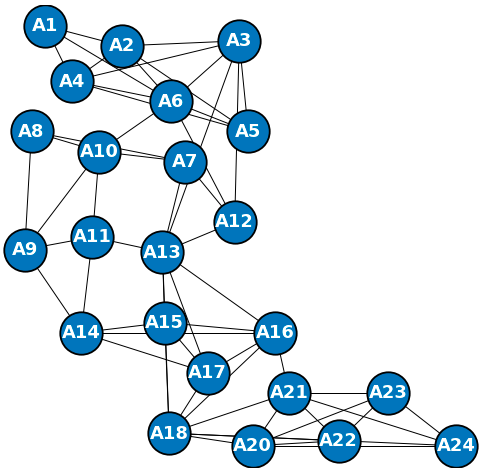
(a) IoT network topology.

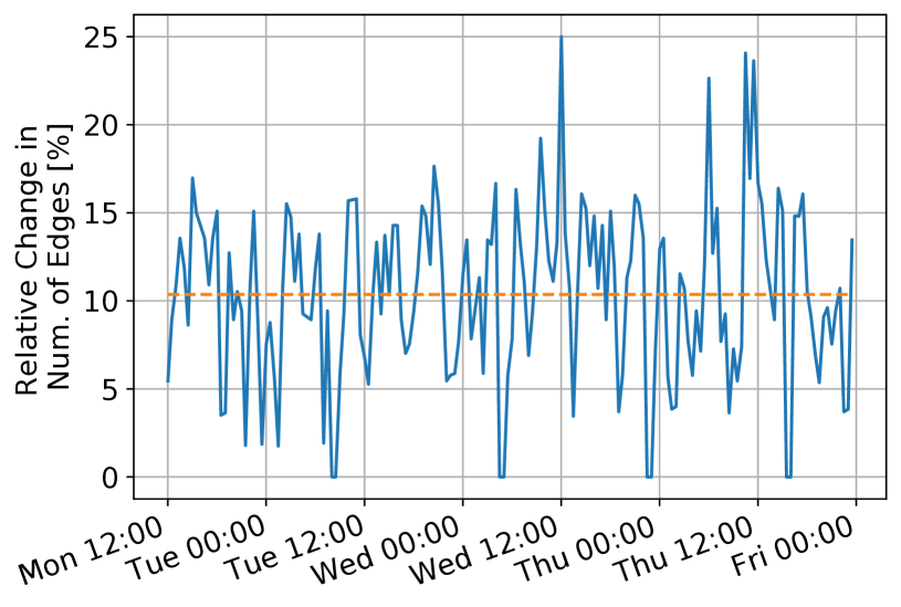
(b) Link connectivity change over time.

Figure 12. We implement DeepGANTT to compute schedules for a real IoT network. The network exhibits a high rate of change in its connectivity between two subsequent link collection time periods. The orange dashed line in 12(b) shows an average of $10.4\%$.

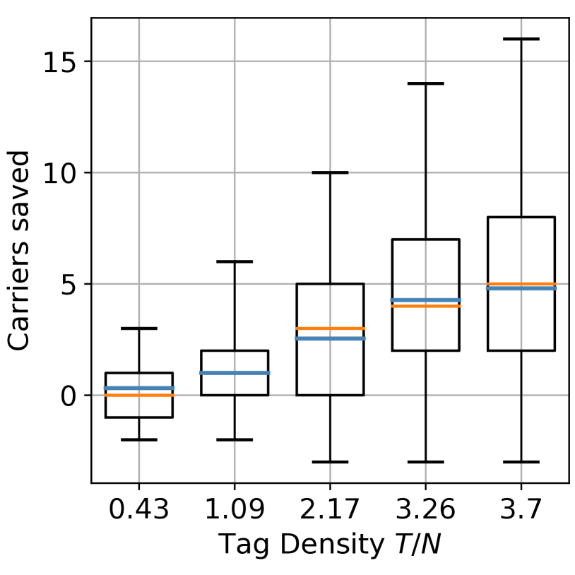
(a) Carriers saved compared to TagAlong heuristic.

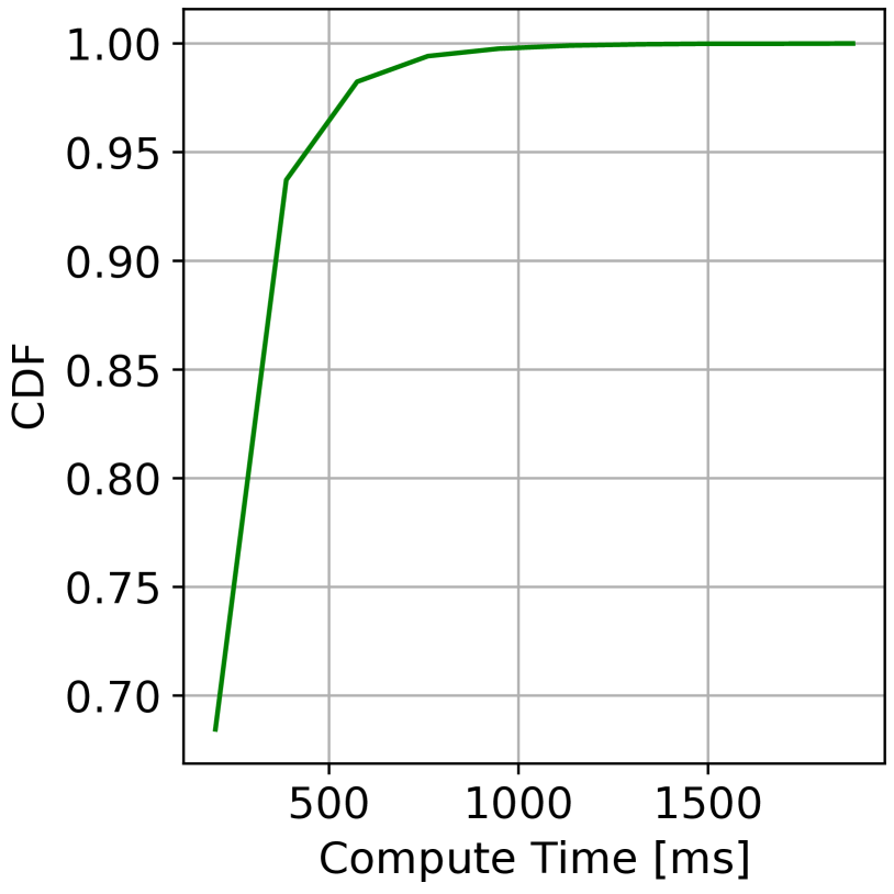
(b) DeepGANTT’s runtime across all tag densities.

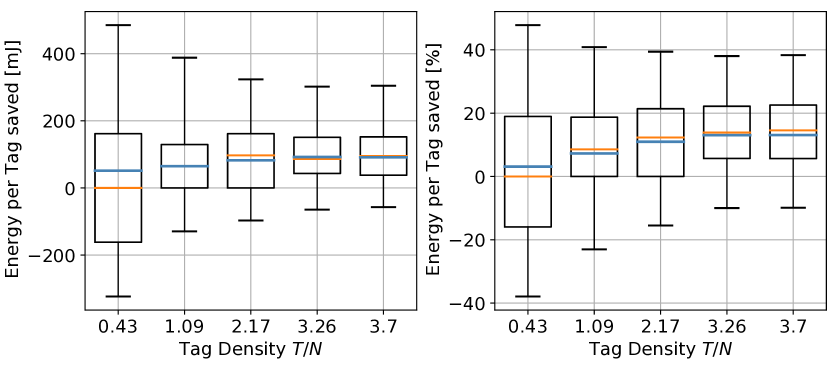
(c) DeepGANTT achieves $13\%$ in average and up to $51\%$ reduction of per-tag energy consumption compared to TagAlong for high tag densities.

Figure 13. DeepGANTT achieves high energy savings compared to TagAlong, even for high tag densities. We successfully deployed DeepGANTT to compute interrogation schedules for a real IoT network of $N\!=\!24$ nodes and varying number of tags $T$. The blue and the orange line represent the mean and the median, respectively. Box extents delimit 25 and 75 percentiles. Whiskers delimit 5 and 99 percentiles.

7. Related Work & Discussion

Our work is relevant both for scheduling in backscatter networks and for supervised ML applied to communications; in particular, to problems of a combinatorial nature.

Many recent related efforts advance backscatter communications and battery-free networks (Kellogg et al., 2016; Talla et al., 2017; Iyer et al., 2016; Ensworth and Reynolds, 2015; Kellogg et al., 2014; Zhang et al., 2017; Majid et al., 2019; Nikitin et al., 2012; Karimi et al., 2017; Geissdoerfer and Zimmerling, 2021), but few of these address the efficient provision of unmodulated carriers. Pérez-Penichet et al. demonstrate TagAlong, a complete system with a polynomial-time heuristic to compute interrogation schedules for backscatter devices (Pérez-Penichet et al., 2020, 2020). Like our work, TagAlong exploits knowledge of the structural properties of the wireless network for fast scheduling. However, TagAlong’s carefully designed algorithm produces wasteful suboptimal schedules. Van Huynh et al. (Huynh et al., 2018) employ numerical analysis to optimize RF energy harvesting tags. By contrast, our work focuses on communication aspects and remains independent of the energy harvesting modality. Carrier scheduling resembles the Reader Collision Problem in RFID systems (Yang et al., 2011; Hamouda et al., 2011; Yue et al., 2012) in that both need to avoid carrier collisions. These works focus on the monostatic backscatter configuration (co-located carrier generator and receiver), whereas our work focuses on the bi-static configuration (separated carrier generators and receivers). The bi-static setting leads to a different optimization problem and our focus is on resource optimization rather than mere collision avoidance.

Previous efforts in communications employ reinforcement learning with GNNs to solve combinatorial scheduling problems, mostly on fixed-size networks or static environments (Wang et al., 2019; Zhang et al., 2019; Bhattacharyya et al., 2019). By contrast, our work focuses on a single solution tackling variable-size inputs and outputs, adequate for a multitude of varying conditions. Also novel in our work is that we employ supervised ML to solve the COP; to the best of our knowledge, this is a new approach within backscatter communications. Yet another novelty in our work is our strategy of restricting the solution space of the COP to boost the trained model’s performance and scalability properties.

ML methods have been applied to COPs over graphs in the past years (Vesselinova et al., 2020), for both reinforcement (Dai et al., 2017; Manchanda et al., 2020) and supervised learning (Vinyals et al., 2015; Li et al., 2018). Similar to our work, Vinyals et al. (Vinyals et al., 2015) implement an attention-based sequence-to-sequence model that learns from optimal solutions to solve the traveling salesperson problem. Likewise, Li et al. (Li et al., 2018) employ GNNs (Kipf and Welling, 2017; Defferrard et al., 2016) to solve three traditional COPs with a supervised approach.

Our symmetry-breaking approach introduces bias in the scheduler: nodes with lower IDs would deplete their batteries faster, given that they will be selected first as carrier generators. Far from a drawback, we believe this can be exploited as a feature at the application level. For instance, one could load-balance carrier scheduling over time, or schedule mains-powered carrier generators whenever possible instead of battery-powered ones simply by ordering the IDs in descending order of priority.

Finally, we believe that our approach to deal with multiple solutions in the scheduling problem could have far-reaching implications in solving the broad class of graph-related NP-hard COPs (such as traveling salesperson) using supervised ML techniques.

8. Conclusion

DeepGANTT is a scheduler that employs GNNs to schedule a network of IoT devices interoperating with battery-free backscatter tags. DeepGANTT leverages self-attention GNNs to overcome the challenges posed by the graph representing the problem and by variable-size inputs and outputs. Our symmetry-breaking strategy succeeds in training DeepGANTT to mimic the behavior of an optimal scheduler. DeepGANTT exhibits strong generalization capabilities to problem instances up to six times larger than those used in training and can compute schedules, requiring on average $7\text{\,}\mathrm{\char 37\relax}\text{/}10\text{\,}\mathrm{\char 37\relax}\text{/}$ and up to $50\%$ fewer carriers than an existing, carefully crafted heuristic, even for the largest problem instances considered. More importantly, our scheduler performs within 3% of the optimal on the average number of carrier slots but with polynomial time complexity; lowering computation times from hours to fractions of a second. Our work advances the development of practical and more efficient backscatter networks. This, in turn, paves the way for wider employment in a large range of environments that today pose problems of great difficulty and importance.

References

- (1)
- Ba et al. (2016) Jimmy Lei Ba, Jamie Ryan Kiros, and Geoffrey E. Hinton. 2016. Layer Normalization. In Proc. Advances NIPS 2016 Deep Learn. Symp. NIPS. arXiv:1607.06450
- Bhattacharyya et al. (2019) Rajarshi Bhattacharyya, Archana Bura, Desik Rengarajan, Mason Rumuly, Srinivas Shakkottai, Dileep Kalathil, Ricky K. P. Mok, and Amogh Dhamdhere. 2019. QFlow: A Reinforcement Learning Approach to High QoE Video Streaming over Wireless Networks. Proc Int. Symp. Mobile Ad Hoc Netw. Comput. (MobiHoc), 251–260. arXiv:1901.00959
- Bishop and Nasrabadi (2006) Christopher M Bishop and Nasser M Nasrabadi. 2006. Pattern recognition and machine learning. Springer.
- Bluetooth SIG (2021) Bluetooth SIG. 2021. Bluetooth Core Specification 5.3.
- Dai et al. (2017) Hanjun Dai, Elias B. Khalil, Yuyu Zhang, Bistra Dilkina, and Le Song. 2017. Learning Combinatorial Optimization Algorithms over Graphs. In Proc. Advances Neural Inf. Process. Syst. (NIPS), Vol. 2017-Decem. Neural information processing systems foundation, 6349–6359. arXiv:1704.01665
- Defferrard et al. (2016) Michaël Defferrard, Xavier Bresson, and Pierre Vandergheynst. 2016. Convolutional Neural Networks on Graphs with Fast Localized Spectral Filtering. In Proc. Advances in Neural Inf. Process. Syst. (NeurIPS). NeurIPS, 3844–3852. arXiv:1606.09375
- Duquennoy et al. (2017) Simon Duquennoy, Atis Elsts, Beshr Al Nahas, and George Oikonomou. 2017. TSCH and 6TiSCH for Contiki: Challenges, Design and Evaluation. In 2017 13th International Conference on Distributed Computing in Sensor Systems (DCOSS). 11–18. https://doi.org/10.1109/DCOSS.2017.29
- Dwivedi et al. (2020) Vijay Prakash Dwivedi, Chaitanya K. Joshi, Thomas Laurent, Yoshua Bengio, and Xavier Bresson. 2020. Benchmarking Graph Neural Networks. Technical Report. arXiv:2003.00982
- Ensworth and Reynolds (2015) Joshua Ensworth and Matthew S. Reynolds. 2015. Every smart phone is a backscatter reader: Modulated backscatter compatibility with Bluetooth 4.0 Low Energy (BLE) devices. In Proc. Ann. Conf. RFID. IEEE.
- Fey and Lenssen (2019) Matthias Fey and Jan E. Lenssen. 2019. Fast Graph Representation Learning with PyTorch Geometric. In Proc. ICLR Workshop Representation Learn. Graphs Manifolds.
- Geissdoerfer and Zimmerling (2021) Kai Geissdoerfer and Marco Zimmerling. 2021. Bootstrapping Battery-free Wireless Networks: Efficient Neighbor Discovery and Synchronization in the Face of Intermittency. In (NSDI’21). 439–455.
- Gilmer et al. (2017) Justin Gilmer, Samuel S. Schoenholz, Patrick F. Riley, Oriol Vinyals, and George E. Dahl. 2017. Neural Message Passing for Quantum Chemistry. Proc. 34th Int. Conf. Mach. Learn. (ICML) 3 (apr 2017), 2053–2070. arXiv:1704.01212
- Hagberg et al. (2008) Aric A. Hagberg, Daniel A. Schult, and Pieter J. Swart. 2008. Exploring Network Structure, Dynamics, and Function using NetworkX. In Proceedings of the 7th Python in Science Conference, Gaël Varoquaux, Travis Vaught, and Jarrod Millman (Eds.). Pasadena, CA USA, 11 – 15.
- Hamilton (2020) William L Hamilton. 2020. Graph representation learning. Vol. 14. Morgan & Claypool Publishers.
- Hamilton et al. (2017) William L. Hamilton, Rex Ying, and Jure Leskovec. 2017. Inductive Representation Learning on Large Graphs. In Proc. Advances Neural Inf. Process. Syst. (NIPS), Vol. 2017-Decem. Neural information processing systems foundation, 1025–1035.
- Hamouda et al. (2011) Essia Hamouda, Nathalie Mitton, and David Simplot-Ryl. 2011. Reader Anti-collision in dense RFID networks with mobile tags. In 2011 IEEE International Conference on RFID-Technologies and Applications. 327–334. https://doi.org/10.1109/RFID-TA.2011.6068657
- Hessar et al. (2018) Mehrdad Hessar, Ali Najafi, and Shyamnath Gollakota. 2018. NetScatter: Enabling Large-Scale Backscatter Networks. In NSDI’18. USENIX.
- Hester and Sorber (2017) Josiah Hester and Jacob Sorber. 2017. The Future of Sensing is Batteryless, Intermittent, and Awesome. In Proc. 15th ACM Conf. on Embedded Netw. Sensor Syst. (Delft, Netherlands) (SenSys ’17). Association for Computing Machinery, New York, NY, USA, Article 21, 6 pages. https://doi.org/10.1145/3131672.3131699
- Huynh et al. (2018) Nguye Van Huynh, Dinh Thai Hoang, Dusit Niyato, Ping Wang, and Dong In Kim. 2018. Optimal Time Scheduling for Wireless-Powered Backscatter Communication Networks. IEEE Wireless Commun. Lett. 7 (2018), 820–823.
- IEEE (2016) IEEE. 2016. IEEE Standard for Low-Rate Wireless Networks –Amendment 2: Ultra-Low Power Physical Layer.
- Iyer et al. (2016) Vikram Iyer et al. 2016. Inter-Technology Backscatter: Towards Internet Connectivity for Implanted Devices. ACM, 356–369. https://doi.org/10.1145/2934872.2934894
- Jameel et al. (2019) Furqan Jameel, Ruifeng Duan, Zheng Chang, Aleksi Liljemark, Tapani Ristaniemi, and Riku Jantti. 2019. Applications of backscatter communications for healthcare networks. IEEE Network 33, 6 (2019), 50–57.
- Karimi et al. (2017) Y. Karimi, A. Athalye, S. R. Das, P. M. Djurić, and M. Stanaćević. 2017. Design of a backscatter-based Tag-to-Tag system. In 2017 IEEE International Conference on RFID (IEEE RFID). 6–12. https://doi.org/10.1109/RFID.2017.7945579
- Kellogg et al. (2014) Bryce Kellogg et al. 2014. Wi-Fi Backscatter: Internet Connectivity for RF-powered Devices. In Proc. Special Interest Group Data Commun. (SIGCOMM). ACM, New York, NY, USA, 607–618. https://doi.org/10.1145/2619239.2626319
- Kellogg et al. (2016) Bryce Kellogg et al. 2016. Passive Wi-Fi: Bringing Low Power to Wi-Fi Transmissions. In Proc. Symp. Networked Syst. Des. Implementation (NSDI). NSDI, 151–164.
- Kingma and Lei Ba (2015) Diederik P Kingma and Jimmy Lei Ba. 2015. Adam: A Method For Stochastic Optimization. In Proc. Int. Conf. Learn. Representations (ICLR). arXiv:1412.6980v9
- Kipf and Welling (2017) Thomas N. Kipf and Max Welling. 2017. Semi-Supervised Classification with Graph Convolutional Networks. In Proc. 5th Int. Conf. Learn. Representations (ICLR). ICLR. arXiv:1609.02907
- Li et al. (2018) Zhuwen Li, Qifeng Chen, and Vladlen Koltun. 2018. Combinatorial optimization with graph convolutional networks and guided tree search. In Proc. Advances in Neural Inf. Process. Syst. (NeurIPS). 539–548.
- Liu et al. (2013) Vincent Liu et al. 2013. Ambient Backscatter: Wireless Communication out of Thin Air. In Proc. Special Interest Group Data Commun. (SIGCOMM). ACM, 39–50. https://doi.org/10.1145/2486001.2486015
- Majid et al. (2019) A. Y. Majid, M. Jansen, G. O. Delgado, K. S. Yildirim, and P. Pawełłzak. 2019. Multi-hop Backscatter Tag-to-Tag Networks. In Proc. Int. Conf. Comput. Commun. (INFOCOM). IEEE, 721–729. https://doi.org/10.1109/INFOCOM.2019.8737551
- Manchanda et al. (2020) Sahil Manchanda, Akash Mittal, Anuj Dhawan, Sourav Medya, Sayan Ranu, and Ambuj Singh. 2020. Learning Heuristics over Large Graphs via Deep Reinforcement Learning. In Proc. 34th Conf. Neural Inf. Process. Syst. (NIPS). arXiv:1903.03332
- Murphy (2012) Kevin P Murphy. 2012. Machine learning: a probabilistic perspective. MIT press.
- Nethercote et al. (2007) Nicholas Nethercote, Peter J. Stuckey, Ralph Becket, Sebastian Brand, Gregory J. Duck, and Guido Tack. 2007. MiniZinc: Towards a standard CP modelling language. In Lecture Notes in Computer Science, Vol. 4741 LNCS. Springer Verlag, 529–543. https://doi.org/10.1007/978-3-540-74970-7_38
- Nikitin et al. (2012) P. V. Nikitin, S. Ramamurthy, R. Martinez, and K. V. S. Rao. 2012. Passive tag-to-tag communication. In Proc. Int. Conf. RFID (RFID). IEEE, 177–184. https://doi.org/10.1109/RFID.2012.6193048
- Oikonomou et al. (2022) George Oikonomou, Simon Duquennoy, Atis Elsts, Joakim Eriksson, Yasuyuki Tanaka, and Nicolas Tsiftes. 2022. The Contiki-NG open source operating system for next generation IoT devices. SoftwareX 18 (2022), 101089. https://doi.org/10.1016/j.softx.2022.101089
- Paszke et al. (2019) Adam Paszke, Sam Gross, Francisco Massa, Adam Lerer, James Bradbury, Gregory Chanan, and et al. 2019. PyTorch: An Imperative Style, High-Performance Deep Learning Library. In Proc. Advances Neural Inf. Process. Syst., H. Wallach, H. Larochelle, A. Beygelzimer, F. d'Alché-Buc, E. Fox, and R. Garnett (Eds.). Curran Associates, Inc., 8024–8035.
- Pérez-Penichet et al. (2016) Carlos Pérez-Penichet, Frederik Hermans, Ambuj Varshney, and Thiemo Voigt. 2016. Augmenting IoT networks with backscatter-enabled passive sensor tags. In Proc. Annu. Int. Conf. Mobile Comput. Netw. (MOBICOM). ACM, 23–27. https://doi.org/10.1145/2980115.2980132
- Pérez-Penichet et al. (2020) Carlos Pérez-Penichet, Dilushi Piumwardane, Christian Rohner, and Thiemo Voigt. 2020. A Fast Carrier Scheduling Algorithm for Battery-free Sensor Tags in Commodity Wireless Networks. In Proc. Int. Conf. Comput. Commun. (INFOCOM). IEEE, 994–1003. https://doi.org/10.1109/infocom41043.2020.9155241
- Perron and Furnon (2019) Laurent Perron and Vincent Furnon. 2019. OR-Tools. https://developers.google.com/optimization/
- Pérez-Penichet et al. (2020) Carlos Pérez-Penichet, Dilushi Piumwardane, Christian Rohner, and Thiemo Voigt. 2020. TagAlong: Efficient Integration of Battery-Free Sensor Tags in Standard Wireless Networks. In Proc. 19th ACM/IEEE Int. Conf. Inf. Process. Sensor Netw. (IPSN). Sydney, Australia. https://doi.org/10.1109/IPSN48710.2020.00020
- Scarselli et al. (2009) Franco Scarselli, Marco Gori, Ah Chung Tsoi, Markus Hagenbuchner, and Gabriele Monfardini. 2009. The graph neural network model. IEEE Trans. Neural Netw. 20, 1 (jan 2009), 61–80. https://doi.org/10.1109/TNN.2008.2005605
- Shi et al. (2021) Yunsheng Shi, Zhengjie Huang, Shikun Feng, Hui Zhong, Wenjing Wang, and Yu Sun. 2021. Masked Label Prediction: Unified Message Passing Model for Semi-Supervised Classification. Technical Report. arXiv:2009.03509v5
- Talla et al. (2017) Vamsi Talla, Mehrdad Hessar, Bryce Kellogg, Ali Najafi, Joshua R. Smith, and Shyamnath Gollakota. 2017. LoRa Backscatter: Enabling The Vision of Ubiquitous Connectivity. Proc. ACM Interact. Mob. Wearable Ubiquitous Technol. 1, 3, 105:1–105:24. https://doi.org/10.1145/3130970
- Varshney et al. (2017) Ambuj Varshney, Carlos Pérez-Penichet, Christian Rohner, and Thiemo Voigt. 2017. LoRea: A Backscatter Architecture That Achieves a Long Communication Range. In Proc. 15th ACM Conf. Embedded Netw. Sensor Syst. (Netherlands) (SenSys ’17). Association for Computing Machinery, New York, NY, USA, Article 50, 2 pages. https://doi.org/10.1145/3131672.3136996
- Vaswani et al. (2017) Ashish Vaswani, Noam Shazeer, Niki Parmar, Jakob Uszkoreit, Llion Jones, Aidan N. Gomez, Łukasz Kaiser, and Illia Polosukhin. 2017. Attention is all you need. In Proc. Advances Neural Inf. Process. Syst. (NIPS), Vol. 2017-Decem. NIPS, 5999–6009.
- Veličković et al. (2018) Petar Veličković, Arantxa Casanova, Pietro Liò, Guillem Cucurull, Adriana Romero, and Yoshua Bengio. 2018. Graph attention networks. In Proc. 6th Int. Conf. Learn. Representations (ICLR). ICLR. arXiv:1710.10903
- Vesselinova et al. (2020) Natalia Vesselinova, Rebecca Steinert, Daniel F Perez-Ramirez, and Magnus Boman. 2020. Learning combinatorial optimization on graphs: A survey with applications to networking. IEEE Access 8 (2020), 120388–120416.
- Vinyals et al. (2015) Oriol Vinyals, Google Brain, Meire Fortunato, and Navdeep Jaitly. 2015. Pointer Networks. In Proc. Advances Neural Inf. Process. Syst. (NIPS). 2692–2700.
- Wang et al. (2019) Fangxin Wang, Cong Zhang, Feng Wang, Jiangchuan Liu, Yifei Zhu, Haitian Pang, and Lifeng Sun. 2019. Intelligent Edge-Assisted Crowdcast with Deep Reinforcement Learning for Personalized QoE. In Proc. IEEE Int. Conf. Comput. Commun. (INFOCOM), Vol. 2019-April. IEEE, 910–918. https://doi.org/10.1109/INFOCOM.2019.8737456
- Wang et al. (2017) Anran Wang et al. 2017. FM Backscatter: Enabling Connected Cities and Smart Fabrics.. In NSDI’17. USENIX, 243–258.
- Winter (2012) T. Winter. 2012. RPL: IPv6 Routing Protocol for Low-Power and Lossy Networks. Retrieved Oct. 2022 from https://www.rfc-editor.org/rfc/rfc6550
- Wu et al. (2021) Zonghan Wu, Shirui Pan, Fengwen Chen, Guodong Long, Chengqi Zhang, and Philip S. Yu. 2021. A Comprehensive Survey on Graph Neural Networks. IEEE Trans. Neural Netw. 32, 1 (2021), 4–24. https://doi.org/10.1109/TNNLS.2020.2978386
- Yang et al. (2011) L. Yang, J. Han, Y. Qi, C. Wang, T. Gu, and Y. Liu. 2011. Season: Shelving interference and joint identification in large-scale RFID systems. In Proc. Int. Conf. Comput. Commun. (INFOCOM). IEEE, 3092–3100. https://doi.org/10.1109/INFCOM.2011.5935154
- You et al. (2019) Jiaxuan You, Rex Ying, and Jure Leskovec. 2019. Position-aware Graph Neural Networks. In Proc. 36th Int. Conf. Mach. Learn. (ICML). arXiv:1906.04817v2
- Yue et al. (2012) H. Yue, C. Zhang, M. Pan, Y. Fang, and S. Chen. 2012. A time-efficient information collection protocol for large-scale RFID systems. In Proc. Int. Conf. Comput. Commun. (INFOCOM). IEEE, 2158–2166. https://doi.org/10.1109/INFCOM.2012.6195599
- Zhang et al. (2019) Han Zhang, Wenzhong Li, Shaohua Gao, Xiaoliang Wang, and Baoliu Ye. 2019. ReLeS: A Neural Adaptive Multipath Scheduler based on Deep Reinforcement Learning. In Proc. Int. Conf. Comput. Commun. (INFOCOM), Vol. 2019-April. IEEE, 1648–1656. https://doi.org/10.1109/INFOCOM.2019.8737649
- Zhang et al. (2017) Pengyu Zhang, Colleen Josephson, Dinesh Bharadia, and Sachin Katti. 2017. FreeRider: Backscatter Communication Using Commodity Radios (CoNEXT ’17). ACM, Incheon, Republic of Korea, 389–401. https://doi.org/10.1145/3143361.3143374