Parameter identifiability of a deep feedforward ReLU neural network

Abstract

The possibility for one to recover the parameters –weights and biases– of a neural network thanks to the knowledge of its function on a subset of the input space can be, depending on the situation, a curse or a blessing. On one hand, recovering the parameters allows for better adversarial attacks and could also disclose sensitive information from the dataset used to construct the network. On the other hand, if the parameters of a network can be recovered, it guarantees the user that the features in the latent spaces can be interpreted. It also provides foundations to obtain formal guarantees on the performances of the network.

It is therefore important to characterize the networks whose parameters can be identified and those whose parameters cannot.

In this article, we provide a set of conditions on a deep fully-connected feedforward ReLU neural network under which the parameters of the network are uniquely identified –modulo permutation and positive rescaling– from the function it implements on a subset of the input space.

Keywords: ReLU networks, Equivalent parameters, Symmetries, Parameter recovery, Deep Learning

1 Introduction

The development of Machine Learning and in particular of Deep Learning in the last decade has led to many breakthroughs in fields such as image classification [30], object recognition [50, 51], speech recognition [26, 53, 24], natural language processing [39, 40, 29], anomaly detection [48] or climate sciences [2]. Deep neural networks are now widely used in real-life tasks stemming from those fields and beyond. This development and the diversity of contexts in which neural networks are used require to investigate theoretical properties that permit to guarantee that they can be used safely, are robust to attack, and can be used widely without giving access to sensitive information.

One key problem in these regards is the relation between the parameters and the function implemented by the network. If a parameterization of a network uniquely defines a function, the reverse is not true. Which other parameterizations define the same function, and what do they have in common? Which information on the parameters of a network are we able to infer from the knowledge of its function on a given domain? Addressing these questions is important for different reasons: industrial property, privacy, robustness and efficiency guarantee (see Section 2 for further discussions and references).

In this article, we consider fully-connected feedforward neural networks with $K$ layers, $K\geq 2$, with the ReLU activation function (see Section 3 for details). The weights and bias parameterizing a neural network are gathered in a list $\mathbf{M}$ of matrices and a list $\mathbf{b}$ of vectors. The corresponding function is denoted $f_{\mathbf{M},\mathbf{b}}:\mathbb{R}^{n_{K}}\longrightarrow\mathbb{R}^{n_{0}}$. We say that two parameterizations $(\mathbf{M},\mathbf{b})$ and $(\tilde{\mathbf{M}},\tilde{\mathbf{b}})$ are equivalent if they can be deduced from each other by the permutation of neurons in each hidden layer and by positive rescaling between the inward and outward weights of every neuron of every hidden layer. These two operations, that are precisely defined in Definition 3, are well-known in the literature [49, 46, 47, 52, 58] and will be referred to as ‘permutation and positive rescaling’. As is well known and restated for completeness in Proposition 4, if two parameterizations $(\mathbf{M},\mathbf{b})$ and $(\tilde{\mathbf{M}},\tilde{\mathbf{b}})$ are equivalent, then the corresponding networks implement the same function: for all $x\in\mathbb{R}^{n_{K}}$, $f_{\mathbf{M},\mathbf{b}}(x)=f_{\tilde{\mathbf{M}},\tilde{\mathbf{b}}}(x)$. In other words, parameter equivalence implies functional equivalence of the networks.

The main contribution of this article is an identifiablity statement (see Theorem 7) which establishes a ‘weak’ converse of this statement. We consider a set $\Omega\subset\mathbb{R}^{n_{K}}$ and two parameterizations $(\mathbf{M},\mathbf{b})$ and $(\tilde{\mathbf{M}},\tilde{\mathbf{b}})$ sharing the same architecture (number of layers and of neurons per layer). We establish a sufficient condition $\mathbf{P}$ such that, if for all $x\in\Omega$, $f_{\mathbf{M},\mathbf{b}}(x)=f_{\tilde{\mathbf{M}},\tilde{\mathbf{b}}}(x)$ and the condition $\mathbf{P}$ is met, then the two parameterizations $(\mathbf{M},\mathbf{b})$ and $(\tilde{\mathbf{M}},\tilde{\mathbf{b}})$ are equivalent. The motivation for the introduction of the set $\Omega$ is that, in practice, we may only test the values of $f_{\mathbf{M},\mathbf{b}}$ and $f_{\tilde{\mathbf{M}},\tilde{\mathbf{b}}}$ on a subset of $\mathbb{R}^{n_{K}}$. Typically, $\Omega$ is a subset of the support of the input distribution law. Such a setting also allows to show that two networks which coincide on a given domain actually coincide on the whole input space $\mathbb{R}^{n_{K}}$. Indeed, if the functions implemented by the networks coincide on $\Omega$ and if the sufficient condition $\mathbf{P}$ is satisfied, then the parameters are equivalent and thus by Proposition 4 the functions also coincide on the rest of the input space $\mathbb{R}^{n_{K}}$. This can be useful to bound the generalization error.

We also reformulate this identifiability statement (see Corollary 8) in a way that illustrates its interest with regard to risk minimization. The corollary considers a random variable $X$ generating the input and an output of the form $Y=f_{\mathbf{M},\mathbf{b}}(X)$, for some parameters $(\mathbf{M},\mathbf{b})$. It states that, when the condition $\mathbf{P}$ is met, any estimated neural network $(\tilde{\mathbf{M}},\tilde{\mathbf{b}})$ for which the population risk equals $0$ belongs to the equivalence class of $(\mathbf{M},\mathbf{b})$. In words, the only way to have a perfect prediction is to perfectly recover $(\mathbf{M},\mathbf{b})$, up to permutation and positive rescaling.

We describe the related works in Section 2. In addition to the works providing identifiability, stability or stable recovery statements, we give a few pointers on privacy, robustness and guarantees of efficiency that motivate our study from an applied perspective. We define in Section 3 the considered neural networks and provide the (known) properties that are useful in our context. The sufficient condition $\mathbf{P}$ and the main theorems are in Section 4. The sketch of the proofs is in Section 5 and the details are in the Appendix.

2 Related work

2.1 Identifiability, stability and stable recovery

2.1.1 Identifiability

Identifiability of the parameters of neural networks has been the topic of a fair amount of work. For smooth activation functions, some results were already established in the 1990s. For shallow networks, results exist for activation functions amongst which $\mathrm{tanh}$ [61, 3], the logistic sigmoid [32], or the Gaussian and rational functions [28]. For deep networks, [18] shows that with $\mathrm{tanh}$ as activation function, with only a few generic conditions on the parameters, two networks that implement the same function have the same architecture and the same parameters up to some permutations and sign-flip operations.

In the case of ReLU networks, we have seen that two operations are well known to preserve the function implemented by the network: permutation and positive rescaling. These operations define equivalence classes on the set of parameters, and we can at best identify the parameters of a network up to these equivalences. It is shown in [47] that these operations are the only generic operations of this kind for ReLU networks with nonincreasing number of neurons per layer. Indeed, they show that for any fully-connected ReLU network architecture with nonincreasing number of neurons per layer, for any nonempty open set $\Omega$, there exists a parameterization $(\mathbf{M},\mathbf{b})$ such that for any other parameterization $(\tilde{\mathbf{M}},\tilde{\mathbf{b}})$ satisfying some generic assumption, if $f_{\tilde{\mathbf{M}},\tilde{\mathbf{b}}}$ coincides with $f_{\mathbf{M},\mathbf{b}}$ on $\Omega$, then $(\tilde{\mathbf{M}},\tilde{\mathbf{b}})$ in the equivalence class of $(\mathbf{M},\mathbf{b})$.

In this work, in order to establish identifiability, we take advantage of the piecewise linear geometry of the functions implemented by ReLU networks to identify the parameters. Indeed, it is well known that the function defined by a deep ReLU network is continuous piecewise-linear, i.e. we can partition the input space into polyhedral regions, sometimes called ‘linear regions’, over which the function is affine. These regions are separated by boundaries that are made of pieces of hyperplanes and that correspond to the non differentiabilities of the function. One crosses such a boundary when the pre-activation value of a neuron (before applying the ReLU function) changes sign. By observing the boundary, one can infer information about the weights and bias of the said neuron.

Other articles adopt similar strategies for shallow [46] or deep networks [52, 47, 58, 59]. The specificity of our proof is to proceed by induction, identifying the weights and bias layer after layer. We discuss the differences between our condition $\mathbf{P}$ and the sufficient conditions given in [47, 52, 59] in detail in Section 4.3.3.

In the case of shallow ReLU networks, [46] establishes a sufficient condition on the parameters for identifiability. If the condition is satisfied by two two-layer fully-connected feedforward ReLU networks whose functions coincide on all the input space, then the parameters of one network can be obtained from the parameters of the other network by permutation and positive rescaling.

In the case of deep ReLU networks, [52] gives a sufficient condition to be able to reconstruct the architecture, weights and biases of a deep ReLU network by knowing its input-output map on all the input space. The condition concerns the boundaries mentioned above: for each neuron in a hidden layer, the authors define the boundary associated to the neuron as the points at which the pre-activation value of the neuron is zero. Then, the condition requires each boundary associated to a neuron in a layer $k$ to intersect the boundaries associated to all the neurons in layer $k+1$ and $k-1$ (see Section 4.3.3 for more details).

Another kind of property is local identifiability, which is identifiability of a parameter $(\mathbf{M},\mathbf{b})$ amongst a set of parameters that are close to $(\mathbf{M},\mathbf{b})$. [59] studies this property for shallow and deep networks. For a deep ReLU network, it first shows that under a trivial assumption, general identifiability up to permutation and positive rescaling implies local identifiability up to positive rescaling, and that the non-existence of ‘twin’ neurons is necessary to identifiability and local identifiability. Then, [59] makes a breakthrough by giving an abstract necessary and sufficient condition on $\mathbf{(M,b)}$ such that there exists a well-chosen finite set $\Omega$ from which local identifiability holds up to positive rescalings, and it gives a bound on the size of the set. Furthermore, more recently, [6] provided a numerically testable condition for local identifiability also from a finite set $\Omega$.

Finally, another line of work that can be linked to identifiability is the field of lossless compression of neural networks [56, 57].

2.1.2 Inverse stability and stable recovery

Establishing identifiability properties is a first step towards establishing inverse stability properties and studying stable recovery algorithms. Given a norm between functions, we say that inverse stability holds when the proximity of the functions implemented by two networks with the same architecture implies the proximity of the corresponding parameters -up to equivalences of parameters, for instance permutations and positive rescalings in the case of ReLU networks. Inverse stability is a stronger property than identifiability, and is necessary for stable recovery algorithms, which goal is to practically recover the parameters of a network from its function.

Inverse stability does not hold in general with the uniform norm for fully-connected feedforward neural networks. Indeed, [45] shows that for any depth, for any architecture with at least 3 neurons in the first hidden layer and any practically used activation function, there exists a sequence of networks whose function tends uniformly to $0$ while any parameterization of these networks tends to infinity.

Many inverse stability and stable recovery results already exist for shallow networks. [17] studies inverse stability directly up to functional equivalence classes, without specifying the nature of these classes in terms of parameters -which interests us in this paper. The authors show that inverse stability has interesting implications in terms of optimization, allowing to link the minima in the parameter space to minima in the realization space (the space of all the functions that can be implemented by a network) and to estimate the quality of local minima in the parameter space based on their radii. Referring to the counter-example given by [45], the authors of [17] argue that the Sobolev norm is more suited than the uniform norm to the problem of inverse stability. With this norm, they concretely establish an inverse stability result on shallow ReLU networks without bias, under a few conditions on the parameters.

When it comes to stable recovery algorithms, [20] provides a sample complexity under which one can recover the parameters of a shallow network with sigmoid activation function using cross-entropy as a loss. For shallow fully-connected ReLU networks, without bias and with Gaussian input, [21, 65, 66, 67] study the stable recovery of the parameters of a teacher network. They give a sample complexity under which minimizing the empirical risk allows to recover the parameters of the network. [34] studies the same configuration but with an identity mapping that skips one layer. ReLU networks can also be used to recover a network with absolute value as activation function [33]. In fact, a neuron with absolute value can be seen as a sum of two ReLU neurons.

Some results also exist in the case of shallow convolutional networks. [8, 64, 63, 16] establish stable recovery results for convolutional ReLU networks with no overlapping. [27] gives a result in the case of a sigmoidal activation function. The case of convolutional ReLU networks with overlapping is studied in [22].

Stability and stable recovery for deep networks is a more complicated question. A few results exist on the subject, but it stays mostly unexplored.

Among them, for deep structured linear networks, [36, 37, 38] use a tensorial lifting technique to establish inverse stability properties. [36, 37] establish necessary and sufficient conditions of inverse stability for a general constraint on the parameters defining the network. [38] specializes the analysis to the sparsity constraint on the parameters, and obtains necessary and sufficient conditions of inverse stability.

The authors of [4] consider deep feed-forward networks with Heavyside activation function which are very sparse and randomly generated. They show that these can be learned with high probability one layer after another.

The authors of [55] consider a deep feed-forward neural network, with an activation function that can be, inter alia, ReLU, sigmoid or softmax. They show that, if the input is Gaussian or its distribution is known, and if the weight matrix of the first layer is sparse, then a method based on moments and sparse dictionary learning can retrieve it exactly. Nothing is said about the stability or the estimation of the other layers.

For deep ReLU networks, in the case where one has full access to the function implemented by the network [52] provides a practical algorithm able to approximately recover the parameters modulo permutation and rescaling, and [9] reconstructs a functionally equivalent network, formulating it as a cryptanalytic problem.

Further inverse stability and stable recovery results for deep ReLU networks are still to be established. Studying identifiability for these networks, as we do in this article, is a first step towards this goal.

2.2 Motivations: privacy, robustness and interpretability

The generalization of deep networks in various applications such as life style choices or medical diagnosis has raised new concerns about privacy and security. Indeed, to perform well, neural networks need to be trained with many examples. The training of some models can take up to several weeks, and need huge datasets such as ImageNet, which contains millions of images. For instance, the training of the giant GPT-3 neural network costed an estimated 12 millions of dollars [7]. For this reason, trained models are valuable and their owners may want to protect them from replication.

In many applications, the training dataset also contains sensitive information that could be uncovered [43, 35, 10, 19, 14]. It is crucial, to the deployment of the solutions relying on deep networks, to guarantee that this cannot occur. For example, when the system returns a confidence indicator in the prediction or a notion of margin, the Model Inversion Attack described in [19] uncovers learning examples $x$ by maximizing the confidence/margin, under a constraint that $\|f_{\mathbf{M},\mathbf{b}}(x)-y\|\leq\varepsilon$, where $y$ is a target output. In moderate dimension, this can be achieved by simply applying $f_{\mathbf{M},\mathbf{b}}$ several times. In large dimension, the complexity of the computation is too large unless the adversary can compute $\nabla f_{\mathbf{M},\mathbf{b}}(x)$, for any $x$. To perform this computation, the adversary needs to know $(\mathbf{M},\mathbf{b})$. Guaranteeing that the parameters cannot be recovered prevents this. With a slightly different objective, (differential) privacy deep learning also assumes that the adversary has the knowledge of the network parameters [1].

Furthermore, knowing the architecture and parameters of a network could make easier for a malicious user to attack it, for instance with adversarial attacks. Indeed, if some black-box adversarial attacks do exist [60, 54, 15], many of them use the knowledge of the parameters of the network, at least to compute the gradients [62, 23, 31, 44, 11, 42, 41, 5].

For all these reasons, the authors of [12] developed a method of preventing parameters extraction by artificially complexifying the network without changing its global behavior. This method builds on previous works on stable recovery of the parameters of the ReLU networks, and in particular on the fact that the piecewise-linear structure of the functions implemented by such networks can be used to recover the parameters. Further understanding of stable recovery for deep networks could help improve protection methods.

Another interest of our work is interpretability of deep neural networks. In some uses of deep networks we want to understand what happens at a layer level and how we can interpret the feature spaces defined by the different layers. But such an interpretation is more meaningful if we know that, for a given function implemented by the network, the parameterization is unique -up to elementary operations such as permutations and positive rescalings for ReLU networks.

3 Neural networks

In this section, we provide known definitions and properties of neural networks with ReLU activation functions. For a self-contained reading, all the corresponding proofs are provided in the appendix.

3.1 Parameterization of neural networks

We consider deep feedforward ReLU networks with $K\geq 2$ layers. To clarify any ambiguity, note that the input layer is not actually counted, as it does not gather any weights. As evoked in the introduction, we index the layers of a deep neural network in reverse order, from $K$ to $0$, for some $K\geq 2$. The input layer is the layer $K$, the output layer is the layer $0$, and between them are $K-1$ hidden layers. We denote by $n_{k}\in\mathbb{N}^{*}$ the number of neurons of the layer $k$. The information contained at the layer $k$ is a $n_{k}$-dimensional vector.

Let $k\in\llbracket 0,K-1\rrbracket$. We denote the weights between the layer $k+1$ and the layer $k$ with a matrix $M^{k}\in\mathbb{R}^{n_{k}\times n_{k+1}}$. We also consider a bias vector $b^{k}\in\mathbb{R}^{n_{k}}$ at the layer $k$, and the ReLU activation function, that is $\sigma(x)=\max(x,0)$. By extension, for a vector $x=(x_{1},\dots,x_{p})^{T}\in\mathbb{R}^{p}$ we also write $\sigma(x)=(\sigma(x_{1}),\dots,\sigma(x_{p}))^{T}$. We denote by $h_{k}$ the mapping implemented by the network between the layer $k+1$ and the layer $k$. If $x\in\mathbb{R}^{n_{k+1}}$ is the information contained at the layer $k+1$, the information contained at the layer $k$ is:

$$h_{k}(x)=\begin{cases}\sigma(M^{k}x+b^{k})&\text{if }k\neq 0\\ M^{k}x+b^{k}&\text{if }k=0.\end{cases}$$ (1)

The parameters of the network can be summarized in the couple $(\mathbf{M},\mathbf{b})$, where $\mathbf{M}=(M^{0},M^{1},\dots,M^{K-1})\in\mathbb{R}^{n_{0}\times n_{1}}\times\dots\times\mathbb{R}^{n_{K-1}\times n_{K}}$ and $\mathbf{b}=(b^{0},b^{1},\dots,b^{K-1})\in\mathbb{R}^{n_{0}}\times\dots\times\mathbb{R}^{n_{K-1}}$. The function implemented by the network is then $f_{\mathbf{M},\mathbf{b}}=h_{0}\circ h_{1}\circ\dots\circ h_{K-1}$, from $\mathbb{R}^{n_{K}}$ to $\mathbb{R}^{n_{0}}$. We refer to Figure 1 for a representation of a neural network and its parameters.

Figure 1: The parameters $\mathbf{M}$ and $\mathbf{b}$ of a neural network.

3.2 Continuous piecewise linear functions and neural networks

We will actively use the fact that the function implemented by a deep ReLU network as well as the intermediate functions between layers are continuous piecewise linear, which means that we can partition their domain of definition in closed polyhedral subsets such that they are linear on each subset. In this paper we use indifferently ‘linear’ or ‘affine’ to describe functions of the form $x\mapsto Ax+b$, with $A\in\mathbb{R}^{n\times m}$ some matrix and $b\in\mathbb{R}^{n}$ some vector.

More precisely, for $m\in\mathbb{N}$, a subset $D\subset\mathbb{R}^{m}$ is a closed polyhedron iif there exist $q\in\mathbb{N}$, $a_{1},\dots,a_{q}\in\mathbb{R}^{m}$ and $b_{1},\dots b_{q}\in\mathbb{R}$ such that for all $x\in\mathbb{R}^{m}$,

$$x\in D\quad\Longleftrightarrow\quad\begin{cases}a_{1}^{T}x+b_{1}\leq 0\\ \vdots\\ a_{q}^{T}x+b_{q}\leq 0.\end{cases}$$ (2)

By convention, if $q=0$, we obtain an empty system of equations which is satisfied for any $x\in\mathbb{R}^{m}$, meaning the set $\mathbb{R}^{m}$ is a closed polyhedron.

We say that a function $g:\mathbb{R}^{m}\rightarrow\mathbb{R}^{n}$ is continuous piecewise linear if there exists a finite set of closed polyhedra whose union is $\mathbb{R}^{m}$ and such that $g$ is linear over each polyhedron.

It is easy to show (see Proposition 19 in the appendix) that this definition implies the continuity of the function, hence the ‘continuous’ in the name. We do not require here the polyhedra to be disjoint and in fact, there are always some overlaps between the borders of adjacent polyhedra. For a given continuous piecewise linear function $g$, there are infinitely many possible sets of closed polyhedra that match the definition. Among them, we can always find one such that all the polyhedra $D$ have nonempty interior $\ring{D}$ (see Proposition 22 in the appendix). We call such a set admissible, as in the following definition.

Definition 1.

Let $g:\mathbb{R}^{m}\rightarrow\mathbb{R}^{n}$ be a continuous piecewise linear function. Let $\Pi$ be a set of closed polyhedra of $\mathbb{R}^{m}$. We say that $\Pi$ is admissible with respect to $g$ if and only if:

$$\begin{cases}\bigcup_{D\in\Pi}D=\mathbb{R}^{m},\\ \text{for all }D\in\Pi,\ g\text{ is linear on }D,\\ \text{for all }D\in\Pi,\ \ring{D}\neq\emptyset.\end{cases}$$ (3)

We now define additional functions associated to a network. Recall the layer functions $h_{k}$ defined in (1), that represent the actions of the network between successive layers. Let $k\in\llbracket 0,K\rrbracket$. We define the following functions:

$$f_{k} =h_{k}\circ h_{k+1}\circ\dots\circ h_{K-1};$$ (4)

$$g_{k} =h_{0}\circ h_{1}\circ\dots\circ h_{k-1}.$$

Above, by convention, we let $f_{K}=id_{\mathbb{R}^{n_{K}}}$ and $g_{0}=id_{\mathbb{R}^{n_{0}}}$, where $id_{\mathbb{R}^{m}}$ denotes the identity function on $\mathbb{R}^{m}$. The function $f_{k}:\mathbb{R}^{n_{K}}\mapsto\mathbb{R}^{n_{k}}$ represents the mapping implemented by the network between the input layer and the layer $k$. The function $g_{k}:\mathbb{R}^{n_{k}}\mapsto\mathbb{R}^{n_{0}}$ represents the mapping implemented by the network between the layer $k$ and the output layer. Hence, for all $k\in\llbracket 0,K\rrbracket$ we have $g_{k}\circ f_{k}=f_{\mathbf{M},\mathbf{b}}$, and in particular $f_{0}=g_{K}=f_{\mathbf{M},\mathbf{b}}$.

For any $\Omega\subset\mathbb{R}^{n_{K}}$, we also denote for all $k\in\llbracket 0,K\rrbracket$,

$$\Omega_{k}=f_{k}(\Omega).$$ (5)

In particular, $\Omega_{K}=f_{K}(\Omega)=\Omega$.

The following proposition is easy to show by induction and using the fact that the composition of two continuous piecewise linear functions is also continuous piecewise linear (see Proposition 32 in the appendix).

Proposition 2.

For all $k\in\llbracket 0,K\rrbracket$, $f_{k}$ and $g_{k}$ are continuous piecewise linear.

In particular, $f_{\mathbf{M,b}}$ is continuous piecewise linear.

We say that a list of sets of closed polyhedra $\boldsymbol{\Pi}=(\Pi_{1},\dots,\Pi_{K-1})$ is admissible with respect to $(\mathbf{M},\mathbf{b})$ iif for all $k\in\llbracket 1,K-1\rrbracket$, the set of closed polyhedra $\Pi_{k}$ is admissible with respect to $g_{k}$. Since there always exist such $\Pi_{k}$ (from Proposition 2 and Proposition 22 in Appendix A), there always exists an admissible list $\mathbf{\Pi}$.

3.3 Equivalence between two parameterizations

We are interested in sufficient conditions to identify the parameters of a network from its function. As mentioned in the introduction, some elementary operations on the parameters are well known to preserve the function of a network, so what we shall actually identify is the equivalence class of the parameters modulo these operations. There are two such operations:

• the permutation of neurons of a hidden layer;

• the positive rescalings, that is, multiplying all the outward weights of a hidden neuron by a strictly positive number and dividing the inward weights by the same number.

The invariance to permutation is classical and common to many feedforward architectures. It is described in the foundational articles [25, 13]. The invariance to positive rescalings is more specific to ReLU (and homogeneous activation functions), and is also well-studied, as for instance in [49, 46, 47, 52, 58].

We give in Definition 3 below the formalization we use for the equivalence relation modulo these operations, after introducing some notations. For all $m\in\mathbb{N}^{*}$, we denote by $\mathfrak{S}_{m}$ the set of all permutations of $\llbracket 1,m\rrbracket$. For any permutation $\varphi\in\mathfrak{S}_{m}$, we denote by $P_{\varphi}$ the $m\times m$ permutation matrix associated to $\varphi$, whose coefficients are defined as

$$(P_{\varphi})_{i,j}=\begin{cases}1&\text{if }\varphi(j)=i\\ 0&\text{otherwise.}\end{cases}$$

We also denote by $\mathbf{1}_{m}$ the vector $(1,1,\dots,1)^{T}\in\mathbb{R}^{m}$, by $\mathbb{R}^{*}_{+}$ the set of strictly positive real numbers and by $\operatorname{Id}_{m}$ the $m\times m$ identity matrix.

Definition 3 (Equivalence between parameters).

If $(\mathbf{M},\mathbf{b})$ and $(\tilde{\mathbf{M}},\tilde{\mathbf{b}})$ are two parameterizations of a network, we say that $(\mathbf{M},\mathbf{b})$ is equivalent to $(\tilde{\mathbf{M}},\tilde{\mathbf{b}})$, and we write $(\mathbf{M},\mathbf{b})\sim(\tilde{\mathbf{M}},\tilde{\mathbf{b}})$, if and only if there exist:

• a family of permutations $\boldsymbol{\varphi}=(\varphi_{0},\dots,\varphi_{K})\in\mathfrak{S}_{n_{0}}\times\dots\times\mathfrak{S}_{n_{K}}$, with $P_{\varphi_{0}}=\operatorname{Id}_{n_{0}}$ and $P_{\varphi_{K}}=\operatorname{Id}_{n_{K}}$,

• a family of vectors $\boldsymbol{\lambda}=(\lambda^{0},\lambda^{1},\dots,\lambda^{K})\in(\mathbb{R_{+}^{*}})^{n_{0}}\times\dots\times(\mathbb{R_{+}^{*}})^{n_{K}}$, with $\lambda^{0}=\mathbf{1}_{n_{0}}$ and $\lambda^{K}=\mathbf{1}_{n_{K}}$,

such that for all $k\in\llbracket 0,K-1\rrbracket$,

$$\begin{cases}\tilde{M}^{k}=P_{\varphi_{k}}\operatorname{Diag}(\lambda^{k})M^{k}\operatorname{Diag}(\lambda^{(k+1)})^{-1}P_{\varphi_{k+1}}^{-1}\\ \tilde{b}^{k}=P_{\varphi_{k}}\operatorname{Diag}(\lambda^{k})b^{k}.\end{cases}$$ (6)

The relation $\mathbf{(M,b)}\sim\mathbf{(\tilde{M},\tilde{b})}$ is an equivalence relation [49, 46, 47]. We include a proof of this fact for completeness in Appendix A (see Proposition 38). We denote by $[\mathbf{M},\mathbf{b}]$ the equivalence class of $(\mathbf{M},\mathbf{b})$.

We can now formalize in Proposition 4 the fact discussed at the beginning of the section: two equivalent parameterizations modulo permutation and positive rescaling implement the same function. As mentioned, this result is well-known [49, 46, 47, 52, 58], but we prove it for completeness in Appendix A (see Proposition 39 and Corollary 40).

Proposition 4.

If $(\mathbf{M},\mathbf{b})\sim(\mathbf{\tilde{M}},\mathbf{\tilde{b}})$, then $f_{\mathbf{M},\mathbf{b}}=f_{\mathbf{\tilde{M}},\mathbf{\tilde{b}}}$.

In this article we give a set of conditions under which we have a reciprocal, i.e. if two parameterizations $(\mathbf{M},\mathbf{b})$ and $(\mathbf{\tilde{M}},\mathbf{\tilde{b}})$ satisfying the conditions lead to the same function on a set $\Omega$, i.e. $f_{\mathbf{M,b}}(x)=f_{\mathbf{\tilde{M},\tilde{b}}}(x)$ for all $x\in\Omega$, then they are equivalent: $\mathbf{(M,b)}\sim\mathbf{(\tilde{M},\tilde{b})}$.

4 Main result

The core of our work is exposed in this section. It is structured as follows. In Section 4.1, we expose the conditions $\mathbf{P}$ and in Section 4.2 we state our main theorems of identifiability. Then, Section 4.3 is dedicated to an extensive discussion of the conditions $\mathbf{P}$, with motivating examples and comparison to the state of the art.

4.1 Conditions

We expose in this section the conditions under which the main theorem holds. They are formalized in Definition 5 and referred to as conditions $\mathbf{P}$.

First, we introduce a few notations. We consider a network with $K\geq 2$ layers and with parameters $\mathbf{(M,b)}$, a list of sets of closed polyhedra $\boldsymbol{\Pi}=(\Pi_{1},\dots,\Pi_{K-1})$ admissible with respect to $\mathbf{(M,b)}$ and a domain $\Omega\subset\mathbb{R}^{n_{K}}$. Recall the definitions (1) and (4) of the functions $h_{k}$, $f_{k}$ and $g_{k}$ associated to the network. For all $k\in\llbracket 1,K-1\rrbracket$, $g_{k}$ is continuous piecewise linear, and since $\boldsymbol{\Pi}$ is admissible with respect to $\mathbf{(M,b)}$, by definition, the set of closed polyhedra $\Pi_{k}$ is admissible with respect to $g_{k}$ in the sense of Definition 1. For all $D\in\Pi_{k}$, the function $g_{k}$ thus coincides with a linear function on $D$. Since by definition the interior of $D$ is nonempty, we define $V^{k}(D)\in\mathbb{R}^{n_{0}\times n_{k}}$ and $c^{k}(D)\in\mathbb{R}^{n_{0}}$ as the unique couple satisfying, for all $x\in D$:

$$g_{k}(x)=V^{k}(D)x+c^{k}(D).$$ (7)

For $\Omega\subset\mathbb{R}^{n_{K}}$, recall the definition (29) of $\Omega_{k}$, for all $k\in[0,K]$. For any $m,n\in\mathbb{N}^{*}$, for any $m\times n$ matrix $\Sigma$, for any $i\in\llbracket 1,m\rrbracket,j\in\llbracket 1,n\rrbracket$, we denote by $\Sigma_{i,.}$ the $i^{\text{th}}$ row vector of $\Sigma$ and by $\Sigma_{.,j}$ the $j^{\text{th}}$ column vector of $\Sigma$. We denote $E^{k}_{i}=\{x\in\mathbb{R}^{n_{k}},\ x_{i}=0\}$, and $h_{k}^{lin}(x)=M^{k}x+b^{k}$. For any $m\in\mathbb{N}^{*}$ and any subset $A\subset\mathbb{R}^{m}$, we denote by $\partial A$ the topological boundary with respect to the standard topology of $\mathbb{R}^{m}$.

Definition 5.

We say that $(\mathbf{M},\mathbf{b},\Omega,\boldsymbol{\Pi})$ satisfies the conditions $\mathbf{P}$ iif for all $k\in\llbracket 1,K-1\rrbracket$:

• $M^{k}$ is full row rank;

• for all $i\in\llbracket 1,n_{k}\rrbracket$, there exists $x\in\ring{\Omega}_{k+1}$ such that

  $$M^{k}_{i,.}x+b^{k}_{i}=0,$$

  or equivalently

  $$E_{i}^{k}\cap h_{k}^{lin}(\ring{\Omega}_{k+1})\neq\emptyset;$$

• for all $D\in\Pi_{k}$, for all $i\in\llbracket 1,n_{k}\rrbracket$, if $E^{k}_{i}\cap D\cap\Omega_{k}\neq\emptyset$ then $V^{k}_{.,i}(D)\neq 0$;

• for any affine hyperplane $H\subset\mathbb{R}^{n_{k+1}}$,

  $$H\cap\ring{\Omega}_{k+1}\ \not\subset\bigcup_{D\in\Pi_{k}}\partial h_{k}^{-1}(D).$$

The conditions $\mathbf{P}$ are invariant modulo equivalences of parameters. Indeed, as shown by the following proposition, if some parameters $\mathbf{(M,b)}$ satisfy the conditions $\mathbf{P}$, then all the parameters in their equivalence class satisfy them too.

Proposition 6.

Suppose $(\mathbf{M},\mathbf{b})$ and $(\mathbf{\tilde{M}},\mathbf{\tilde{b}})$ are two equivalent network parameterizations, and suppose that there exists a list $\boldsymbol{\Pi}$ admissible with respect to $(\mathbf{M},\mathbf{b})$ such that $(\mathbf{M},\mathbf{b},\Omega,\boldsymbol{\Pi})$ satisfies the conditions $\mathbf{P}$.

Then, there exists a list $\boldsymbol{\tilde{\Pi}}$ that is admissible with respect to $\mathbf{(\tilde{M},\tilde{b})}$, and such that $(\mathbf{\tilde{M}},\mathbf{\tilde{b}},\Omega,\boldsymbol{\tilde{\Pi}})$ satisfies the conditions $\mathbf{P}$.

Proposition 6 is proven as Proposition 50 in Appendix B.

4.2 Main theorems

We have now introduced all the necessary material to expose our main result, Theorem 7, as well as an application in terms of risk minimization in Section 4.2.2.

4.2.1 Identifiability statement

Our main theorem is the following one. We provide a sketch of the proof in Section 5. For the complete proof, see Theorem 51 in Appendix B and its proof in Section B.4.

Theorem 7.

Let $K\in\mathbb{N}$, $K\geq 2$. Suppose we are given two networks with $K$ layers, identical number of neurons per layer, and with respective parameters $(\mathbf{M},\mathbf{b})$ and $(\mathbf{\tilde{M}},\mathbf{\tilde{b}})$. Assume $\boldsymbol{\Pi}$ and $\boldsymbol{\tilde{\Pi}}$ are two lists of sets of closed polyhedra that are admissible with respect to $(\mathbf{M},\mathbf{b})$ and $(\mathbf{\tilde{M}},\mathbf{\tilde{b}})$ respectively. Denote by $n_{K}$ the number of neurons of the input layer, and suppose we are given a set $\Omega\subset\mathbb{R}^{n_{K}}$ such that $(\mathbf{M},\mathbf{b},\Omega,\boldsymbol{\Pi})$ and $(\mathbf{\tilde{M}},\mathbf{\tilde{b}},\Omega,\boldsymbol{\tilde{\Pi}})$ satisfy the conditions $\mathbf{\mathbf{P}}$, and such that, for all $x\in\Omega$:

$$f_{\mathbf{M},\mathbf{b}}(x)=f_{\tilde{\mathbf{M}},\tilde{\mathbf{b}}}(x).$$

Then:

$$(\mathbf{M},\mathbf{b})\sim(\mathbf{\tilde{M}},\mathbf{\tilde{b}}).$$

As mentioned before, this theorem can be seen as a partial reciprocal to Proposition 4. Indeed, the latter shows that two networks with equivalent parameters modulo permutation and positive rescaling implement the same function. In other words, parameter equivalence implies functional equivalence of the networks. In Theorem 7, we state that under the conditions $\mathbf{P}$, functional equivalence (on a given domain $\Omega$) implies parameter equivalence modulo permutation and positive rescaling.

4.2.2 An application to risk minimization

Assume we are given a couple of input-output variables $(X,Y)$ generated by a ground truth network with parameters $(\mathbf{M},\mathbf{b})$:

$$Y=f_{\mathbf{M,b}}(X).$$

We can use Theorem 7 to show that the only way to bring the population risk to $0$ is to find the ground truth parameters -modulo permutation and positive rescaling.

Indeed, let $\Omega\subset\mathbb{R}^{n_{K}}$ be a domain that is contained in the support of $X$, and suppose $L:\mathbb{R}^{n_{0}}\times\mathbb{R}^{n_{0}}\rightarrow\mathbb{R}_{+}$ is a loss function such that $L(y,y^{\prime})=0\Rightarrow y=y^{\prime}$. Consider the population risk:

$$R(\mathbf{\tilde{M}},\mathbf{\tilde{b}})=\mathbb{E}[L(f_{\mathbf{\tilde{M}},\mathbf{\tilde{b}}}(X),Y)].$$

We have the following result.

Corollary 8.

Suppose there exists a list of sets of closed polyhedra $\boldsymbol{\Pi}$ admissible with respect to $(\mathbf{M},\mathbf{b})$ such that $(\mathbf{M},\mathbf{b},\Omega,\boldsymbol{\Pi})$ satisfies the conditions $\mathbf{P}$.

If $(\mathbf{\tilde{M}},\mathbf{\tilde{b}})$ is such that there exists a list $\boldsymbol{\tilde{\Pi}}$ admissible with respect to $(\mathbf{\tilde{M}},\mathbf{\tilde{b}})$ such that $(\mathbf{\tilde{M}},\mathbf{\tilde{b}},\Omega,\boldsymbol{\tilde{\Pi}})$ satisfies the conditions $\mathbf{P}$, and if $(\mathbf{M},\mathbf{b})\not\sim(\mathbf{\tilde{M}},\mathbf{\tilde{b}})$, then:

$$R(\mathbf{\tilde{M}},\mathbf{\tilde{b}})>0.$$

For the proof, see Corollary 52 in Appendix B and its proof in Section B.5.

4.3 Discussion on the conditions

This section is dedicated to discussing the conditions $\mathbf{P}$. We start by explaining the different conditions $\mathbf{P}.a)-\mathbf{P}.d)$ and their purpose in Section 4.3.1. Then, in Section 4.3.2, we provide counter-examples illustrating how non-identifiability arises when they are not satisfied. Finally, we compare the conditions $\mathbf{P}$ to the state of the art in Sections 4.3.3 and 4.3.4.

4.3.1 The conditions explained

Let us explain the conditions $\mathbf{P}$. The first condition, $\mathbf{P}.a)$, requires the matrix $M^{k}\in\mathbb{R}^{n_{k}\times n_{k+1}}$ to have full row rank. This implies that for all $k\in\llbracket 1,K-1\rrbracket$, the layer $k$ has no more neurons than its predecessor, the layer $k+1$:

$$n_{k}\leq n_{k+1}.$$

Once this is satisfied, the condition is mild in the sense that it is satisfied for all matrices except a set of matrices of empty Lebesgue measure.

As a first remark about $\mathbf{P}.b)$, notice that by taking $k=K-1$, it implies that $\ring{\Omega}=\ring{\Omega}_{K}\neq\emptyset$. Thus, in the main result, the set $\Omega$ over which the function implemented by the network is assumed to be known needs to have nonempty interior. In particular, $\Omega$ cannot be a finite sample set. This limitation is already present in [52], which assumes an access to the function on the whole input space and [47] which considers the function of the network on a bounded open nonempty domain. However, as we discuss in the conclusion, it seems possible to establish a result for a finite $\Omega$, and the conditions formulated here should be a basis for future work.

The conditions $\mathbf{P}.b),\mathbf{P}.c)$ and $\mathbf{P}.d)$ must be satisfied for all $k\in\llbracket 1,K-1\rrbracket$, but to give a sense of them, let us see what they mean for $k=K-1$.

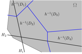
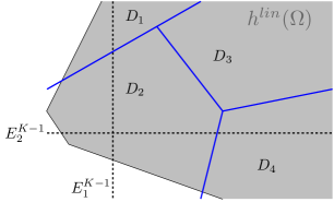
$\mathbb{R}^{n_{K}}$	$\mathbb{R}^{n_{K-1}}$

Figure 2: Left. In $\mathbb{R}^{n_{K}}$, the inverse image by $h_{K-1}$ of the polyhedra $D\in\Pi_{K-1}$. To make the figure lighter we write $h$ instead of $h_{K-1}$. The grey zone represents $\Omega$. For $i\in\{1,2\}$, $H_{i}$ is the hyperplane defined by the equation $M^{K-1}_{i,.}x+b^{K-1}_{i}=0$. As a direct consequence, we have $h(H_{i})\subset E_{i}^{K-1}$. Right. In $\mathbb{R}^{n_{K-1}}$, the admissible polyhedra $D\in\Pi_{K-1}$ with respect to $g_{K-1}$. The grey zone corresponds to the image $h^{lin}(\Omega)=M^{K-1}\Omega+b^{K-1}$.

As explained in Section 3.2, the function implemented by a ReLU network is continuous piecewise linear: we can divide the input space $\mathbb{R}^{n_{K}}$ into polyhedral regions, over each of which the function is linear. We take advantage of this structure to acquire information about the parameters of the network. The boundaries of the polyhedral regions are of particular interest. They are made of pieces of hyperplanes, and they roughly correspond to the points where the function implemented by the network is not differentiable. We use this non differentiability property to identify the boundaries. We go from one linear region to another when there is a change of sign in the pre-activation value (input of $\sigma$) of one hidden neuron. The boundary between two linear regions is thus associated to a particular neuron of a particular hidden layer.

We separate the function implemented by the first layer of the network and the function implemented by the rest of the layers thanks to the functions defined in (1) and (4), writing

$$f_{\mathbf{M},\mathbf{b}}=g_{K}=g_{K-1}\circ h_{K-1},$$

$$\mathbb{R}^{n_{K}}\ \overset{h_{K-1}}{\longrightarrow}\ \mathbb{R}^{n_{K-1}}\ \overset{g_{K-1}}{\longrightarrow}\ \mathbb{R}^{n_{0}}.$$

The goal is first to identify the weights and bias of the first layer, $M^{K-1}$ and $b^{K-1}$. To do so, we focus on the boundaries associated to the neurons in the first hidden layer. These ‘first-order’ boundaries are hyperplanes defined by the equations $M^{K-1}_{i,.}x+b^{K-1}_{i}=0$, for all $i\in\llbracket 1,n_{K-1}\rrbracket$. The conditions $\mathbf{P}.b)$, $\mathbf{P}.c)$ and $\mathbf{P}.d)$ are made to ensure that we are able to identify the hyperplanes, and consequently, the parameters $M^{K-1}$ and $b^{K-1}$. The two relevant spaces to visualize the conditions are the input space, $\mathbb{R}^{n_{K}}$, and the first hidden space, $\mathbb{R}^{n_{K-1}}$, which are represented in Figure 2. Let us explain the conditions $\mathbf{P}.b),\mathbf{P}.c)$ and $\mathbf{P}.d)$.

• The condition $\mathbf{P}.b)$ in the case $k=K-1$ requires the hyperplane defined by the equation $M^{K-1}_{i,.}x+b^{K-1}=0$ to intersect $\ring{\Omega}_{K}=\ring{\Omega}$. Indeed, we only consider the function implemented by the network over $\Omega$, so the hyperplane must intersect $\ring{\Omega}_{K}$ in order to be detectable as a non differentiability. In the example of Figure 2, we see that the two such hyperplanes, which are $H_{1}$ and $H_{2}$, intersect $\Omega$, so the condition is satisfied.

• Consider a polyhedron $D\in\Pi_{K-1}$. The function $g_{K-1}$ is linear over $D$, and using the notations defined in (7), we have for all $u\in D$,

  $$g_{K-1}(u)=V^{K-1}(D)u+c^{K-1}(D).$$ (8)

  For all $x\in\mathbb{R}^{n_{K}}$ such that $h_{K}(x)\in D$, using (8) we obtain:

  $$f_{\mathbf{M},\mathbf{b}}(x)=g_{K-1}\circ h_{K-1}(x)=\sum_{i=1}^{n_{K-1}}V^{K-1}_{.,i}(D)\sigma\left(M^{K-1}_{i,.}x+b^{K-1}_{i}\right)+c^{K-1}(D).$$

  In particular, at the points $x$ such that $M^{K-1}_{i,.}x+b^{K-1}_{i}=0$, the function $\sigma(M^{K-1}_{i,.}x+b^{K-1}_{i})$ is not differentiable, and this non differentiability can only be reflected in the function $f_{\mathbf{M},\mathbf{b}}$ if $V^{K-1}_{.,i}(D)\neq 0$. The condition $\mathbf{P}.c)$ ensures that. In the example of Figure 2 (right part), we see that $D_{1}$ intersects $E^{K-1}_{1}$ so to satisfy $\mathbf{P}.c)$, we must have $V^{K-1}_{.,1}(D_{1})\neq 0$. Similarly, $D_{2}$ intersects $E^{K-1}_{1}$ and $E^{K-1}_{2}$ so we must have $V^{K-1}_{.,1}(D_{2})\neq 0$ and $V^{K-1}_{.,2}(D_{2})\neq 0$, and the polyhedron $D_{4}$ intersects $E_{2}^{K-1}$ so we must have $V^{K-1}_{.,2}(D_{4})\neq 0$.

• For the last condition, $\mathbf{P}.d)$, we consider the inverse images $h_{K-1}^{-1}(D)$, for all the polyhedra $D\in\Pi_{K-1}$. Since $h_{K-1}$ is piecewise linear and $D$ is a closed polyhedron, $h_{K-1}^{-1}(D)$ is a finite union of closed polyhedra (see the first point of Proposition 23 in the appendix). In particular, its boundary $\partial h_{K-1}^{-1}(D)$ is made of pieces of hyperplanes. We require the union of these boundaries not to contain any full hyperplane (within the domain $\Omega$). In the example of Figure 2, the condition is satisfied.

4.3.2 Illustrative counter-examples

To illustrate the necessity for the conditions in $\mathbf{P}$, we give for each of the conditions $\mathbf{P}.a)-\mathbf{P}.d)$ a simple example of a parameterization $(\mathbf{M},\mathbf{b})$ and a set $\Omega$ which do not satisfy it, and we show that $(\mathbf{M},\mathbf{b})$ is not identifiable by constructing a parameterization $(\tilde{\mathbf{M}},\tilde{\mathbf{b}})$ that is not equivalent to $(\mathbf{M},\mathbf{b})$, but such that $f_{\tilde{\mathbf{M}},\tilde{\mathbf{b}}}$ coincides with $f_{\mathbf{M},\mathbf{b}}$ over $\Omega$. These four examples illustrate the behaviors we want to prevent with the conditions $\mathbf{P}$.

Example 9.

We consider an architecture with one hidden layer, i.e. $K=2$, with $n_{2}=2$, $n_{1}=3$, $n_{0}=1$. We consider the parameterization $(\mathbf{M},\mathbf{b})$ defined as follows.

$$M^{1}=\begin{pmatrix}0&2\\ 1&-1\\ -1&-1\end{pmatrix}\qquad b^{1}=\begin{pmatrix}0\\ 0\\ 0\end{pmatrix},$$

$$M^{0}=\begin{pmatrix}1&1&1\end{pmatrix}\qquad b^{0}=0.$$

For this example, we consider $\Omega=\mathbb{R}$.

The condition $\mathbf{P}.a)$ is not satisfied: the matrix $M^{1}$ cannot have full row rank since its dimension is $3\times 2$, and more specifically we have the relation

$$M^{1}_{1,.}+M^{1}_{2,.}+M^{1}_{3,.}=0.$$ (9)

Let us define $\tilde{M}^{1}=-M^{1}$ and $\tilde{\mathbf{M}}=(\tilde{M}^{1},M^{0})$. Let us show that $f_{\tilde{\mathbf{M}},\mathbf{b}}=f_{\mathbf{M},\mathbf{b}}$.

Let $x\in\mathbb{R}^{2}$. We have

$$f_{\mathbf{M},\mathbf{b}}(x)=\sigma\left(M^{1}_{1,.}x\right)+\sigma\left(M^{1}_{2,.}x\right)+\sigma\left(M^{1}_{3,.}x\right).$$

There exist activations $\epsilon_{1},\epsilon_{2},\epsilon_{3}\in\{0,1\}$, depending on $x$, such that

$$f_{\mathbf{M},\mathbf{b}}(x)=\epsilon_{1}M^{1}_{1,.}x+\epsilon_{2}M^{1}_{2,.}x+\epsilon_{3}M^{1}_{3,.}x.$$ (10)

Since $\tilde{M}^{1}=-M^{1}$ and $b^{1}=0$, the signs of the activations are switched in $f_{\tilde{\mathbf{M}},\mathbf{b}}$ and thus

$$f_{\tilde{\mathbf{M}},\mathbf{b}}(x) =(1-\epsilon_{1})\tilde{M}^{1}_{1,.}x+(1-\epsilon_{2})\tilde{M}^{1}_{2,.}x+(1-\epsilon_{3})\tilde{M}^{1}_{3,.}x$$

$$=\sum_{i=1}^{3}(1-\epsilon_{i})(-M^{1}_{i,.}x)$$

$$=\sum_{i=1}^{3}\epsilon_{i}M^{1}_{i,.}x-(\sum_{i=1}^{3}M^{1}_{i,.})x$$

$$=f_{\mathbf{M},\mathbf{b}}(x),$$

where we obtain the last equality thanks to (9) and (10).

Now since only the positive rescalings are authorized, $(\tilde{\mathbf{M}},\mathbf{b})$ is not equivalent to $(\mathbf{M},\mathbf{b})$, which shows that $(\mathbf{M},\mathbf{b})$ is not identifiable modulo permutation and rescaling.

Example 10.

Let us consider a very simple architecture with one hidden layer and only one neuron per layer, i.e. $n_{2}=n_{1}=n_{0}=1$. We consider the parameterization $(\mathbf{M},\mathbf{b}_{a})$, for $a>0$, defined by

$$M^{1}=1,\quad b_{a}^{1}=a,\quad M^{0}=1,\quad b_{a}^{0}=-a.$$

The function implemented by the network satisfies, for all $x\in\mathbb{R},$

$$f_{\mathbf{M},\mathbf{b}_{a}}(x)=\sigma(x+a)-a=\begin{cases}-a&\text{if }x<-a\\ x&\text{if }x\geq-a.\end{cases}$$ (11)

Let us consider $\Omega=[1,+\infty[$. With such a choice of $\Omega$, none of the parameterizations $(\mathbf{M},\mathbf{b}_{a})$ satisfy $\mathbf{P}.b)$, because for all $x\in\Omega$, $M^{1}x+b_{a}^{1}=x+a>0$.

For any $a>0$, for any $x\in\Omega$, we have $x\geq 1>-a$, so (11) shows that $f_{\mathbf{M},\mathbf{b}_{a}}(x)=x$, i.e. the functions implemented by the parameterizations $(\mathbf{M},\mathbf{b}_{a})$ all coincide over $\Omega$. However, since (11) shows they do not implement the same function over $\mathbb{R}$, Proposition 4 shows they are not equivalent.

Example 11.

We consider an architecture with $2$ hidden layers, that is $K=3$, and again one neuron per layer: $n_{3}=n_{2}=n_{1}=n_{0}=1$. Let us consider the parameterizations $(\mathbf{M},\mathbf{b}_{a})$, defined for $a>0$ by

$$M^{2}=1,\qquad b^{2}_{a}=a,$$

$$M^{1}=1,\qquad b^{1}_{a}=-1-a,$$

$$M^{0}=1,\qquad b^{0}_{a}=0.$$

We consider $\Omega=\mathbb{R}$. Let us show that for any $a>0$ and any admissible $\boldsymbol{\Pi}$, the condition $\mathbf{P}.c)$ is not satisfied by $(\mathbf{M},\mathbf{b},\Omega,\boldsymbol{\Pi})$ in the case $k=2$.

Indeed, we have $h_{2,a}(x)=\sigma(M^{2}x+b^{2}_{a})=\sigma(x+a)$, and thus $\Omega_{2}=h_{2,a}(\Omega)=\mathbb{R}_{+}$. Further, the expression of $g_{2,a}$ is

$$g_{2,a}(x)=M^{0}\sigma(M^{1}x+b^{1}_{a})+b^{0}_{a}=\sigma(x-1-a)=\begin{cases}0&\text{if }x\leq 1+a\\ x-1-a&\text{if }x>1+a.\end{cases}$$

For any set of closed polyhedra $\Pi_{2}$ admissible with respect to $g_{2,a}$, a polyhedron $D\in\Pi_{2}$ intersecting $E_{1}^{2}=\{0\}$ must satisfy $V^{2}(D)=0$ since $g_{2,a}(x)=0$ for $x\in]-\infty,1+a]$. This contradicts $\mathbf{P}.c)$ for $k=2$.

To exhibit functionally equivalent parameterizations, we now show that for all $a>0$ and $x\in\mathbb{R}$,

$$f_{\mathbf{M},\mathbf{b}_{a}}(x)=\sigma(x-1).$$ (12)

Indeed, let $x\in\mathbb{R}$.

• if $x\in]-\infty,-a[$, we have $\sigma(M^{2}x+b^{2}_{a})=\sigma(x+a)=0$, so

  $$f_{\mathbf{M},\mathbf{b}_{a}}(x) =M^{0}\sigma(M^{1}\cdot 0+b^{1}_{a})+b^{0}_{a}$$

  $$=\sigma(b^{1}_{a})$$

  $$=0=\sigma(x-1).$$

• if $x\in[-a,+\infty[$, we have $\sigma(M^{2}x+b^{2}_{a})=\sigma(x+a)=x+a$, so

  $$f_{\mathbf{M},\mathbf{b}_{a}}(x) =M^{0}\sigma(M^{1}(x+a)+b^{1}_{a})+b^{0}_{a}$$

  $$=\sigma(x+a-1-a)$$

  $$=\sigma(x-1).$$

This shows (12). The function $f_{\mathbf{M},\mathbf{b}_{a}}$ is therefore independent of $a>0$, but if $a\neq a^{\prime}$, $(\mathbf{M},\mathbf{b}_{a})\not\sim(\mathbf{M},\mathbf{b}_{a^{\prime}})$.

The lack of identifiability comes here from the fact that we do not ‘observe’ the non differentiability induced by the first hidden neuron, because $V^{2}(D)=0$ for $D$ containing $0$. Indeed, if $\mathbf{P}.c)$ was satisfied, we would observe a non differentiability at the point at which the sign of $M^{2}x+b_{a}^{2}$ changes, which is $x=-a$, and we thus would have $f_{\mathbf{M},\mathbf{b}_{a}}\neq f_{\mathbf{M},\mathbf{b}_{a^{\prime}}}$ for $a\neq a^{\prime}$.

We remark that here, even if $\mathbf{P}.c)$ was satisfied, the condition $\mathbf{P}.d)$ would not be satisfied, as we see next in Example 12.

Example 12.

We consider again the architecture of Example 11, wih two hidden layers and one neuron per layer. This time, we consider the parameterizations $(\mathbf{M},\mathbf{b})$ and $(\tilde{\mathbf{M}},\tilde{\mathbf{b}})$, defined by

$$M^{2}=1, b^{2}=0,$$

$$M^{1}=-1, b^{1}=1,$$

$$M^{0}=-1, b^{0}=0,$$

and

$$\tilde{M}^{2}=-1, \tilde{b}^{2}=1,$$

$$\tilde{M}^{1}=-1, \tilde{b}^{1}=1,$$

$$\tilde{M}^{0}=1, \tilde{b}^{0}=-1.$$

We can remark without waiting further that $(\mathbf{M},\mathbf{b})\not\sim(\tilde{\mathbf{M}},\tilde{\mathbf{b}})$, for instance because $b^{0}=0$, and $\tilde{b}^{0}=-1$, and the rescalings do not permit such a transformation.

Let $\Omega=\mathbb{R}$. Let us consider the sets $\Pi_{2}=\{]-\infty,1],[1,+\infty[\}$, $\Pi_{1}=\{\mathbb{R}\}$ and the list $\boldsymbol{\Pi}=(\Pi_{1},\Pi_{2})$. After showing that $\boldsymbol{\Pi}$ is admissible with respect to $(\mathbf{M},\mathbf{b})$, we will first show that $(\mathbf{M},\mathbf{b})$ does not satisfy the condition $\mathbf{P}.d)$ and we will then show that $f_{\mathbf{M},\mathbf{b}}=f_{\tilde{\mathbf{M}},\tilde{\mathbf{b}}}$.

Let us show that $\boldsymbol{\Pi}$ is admissible with respect to $(\mathbf{M},\mathbf{b})$. Indeed, for all $x\in\mathbb{R}$, we have

$$g_{2}(x)=M^{0}\sigma(M^{1}x+b^{1})+b^{0}=-\sigma(-x+1).$$

The function $g_{2}$ is linear over both the intervals $]-\infty,1]$ and $[1,+\infty[$, so $\Pi_{2}$ is admissible with respect to $g_{2}$. The function $g_{1}$ is linear, so $\Pi_{1}$ is admissible with respect to $g_{1}$.

Let us now show that $(\mathbf{M},\mathbf{b},\Omega,\boldsymbol{\Pi})$ does not satisfy the condition $\mathbf{P}.d)$. Let us first determine $\bigcup_{D\in\Pi_{2}}\partial h_{2}^{-1}(D)$. Since $h_{2}(x)=\sigma(x)$, we have $h_{2}^{-1}(]-\infty,1[)=]-\infty,1]$ and $h_{2}^{-1}([1,+\infty[)=[1,+\infty[$. Hence,

$$\bigcup_{D\in\Pi_{2}}\partial h_{2}^{-1}(D)=\{1\}.$$

Now, since $\ring{\Omega}_{3}=\ring{\Omega}=\mathbb{R}$, we have

$$\ring{\Omega}_{3}\cap\{1\}\subset\bigcup_{D\in\Pi_{2}}\partial h_{2}^{-1}(D),$$

and since $\{1\}$ is an affine hyperplane of $\mathbb{R}$, this shows that $\mathbf{P}.d)$ is not satisfied for $k=2$.

Let us now show that for all $x\in\Omega=\mathbb{R}$, we have

$$f_{\mathbf{M},\mathbf{b}}(x)=f_{\tilde{\mathbf{M}},\tilde{\mathbf{b}}}(x)=\begin{cases}\sigma(x)-1&\mbox{if }x\leq 1\\ 0&\text{if }x>1.\end{cases}$$ (13)

Let us first determine $f_{\mathbf{M},\mathbf{b}}(x)$, for $x\in\mathbb{R}$. We have

$$f_{\mathbf{M},\mathbf{b}}(x)=M^{0}\sigma(M^{1}\sigma(M^{2}x+b^{2})+b^{1})+b^{0}=-\sigma(-\sigma(x)+1).$$

• If $x\leq 1$, then $\sigma(x)\leq 1$ and thus $-\sigma(x)+1\geq 0$. Thus, $-\sigma(-\sigma(x)+1)=\sigma(x)-1$, and $f_{\mathbf{M},\mathbf{b}}(x)=\sigma(x)-1.$

• If $x>1$, then $-\sigma(x)+1<0$ and thus $-\sigma(-\sigma(x)+1)=0$. We thus have $f_{\mathbf{M},\mathbf{b}}(x)=0.$

Let us now determine $f_{\tilde{\mathbf{M}},\tilde{\mathbf{b}}}(x)$, for $x\in\mathbb{R}$. We have

$$f_{\tilde{\mathbf{M}},\tilde{\mathbf{b}}}(x)=\tilde{M}^{0}\sigma(\tilde{M}^{1}\sigma(\tilde{M}^{2}x+\tilde{b}^{2})+\tilde{b}^{1})+\tilde{b}^{0}=\sigma(-\sigma(-x+1)+1)-1.$$

• If $x\leq 1$, then $-x+1\geq 0$ and thus $f_{\tilde{\mathbf{M}},\tilde{\mathbf{b}}}(x)=\sigma((x-1)+1)-1=\sigma(x)-1$.

• If $x>1$, then $-x+1\leq 0$ and thus $f_{\tilde{\mathbf{M}},\tilde{\mathbf{b}}}(x)=\sigma(1)-1=0$.

This shows (13), and as a consequence, $(\mathbf{M},\mathbf{b})$ is not identifiable.

In this example, the lack of identifiability comes from the fact that the sets of non differentiabilities induced by the first and the second layer are indistinguishable: they are both reduced to a point. This will always be the case for networks with only one neuron per layer and more than one hidden layer. When the input dimension is 2 or higher and the condition $\mathbf{P}.d)$ is satisfied, the non differentiabilities induced by neurons in the first hidden layer are the only ones that correspond to full hyperplanes, and this is how they can be identified, as illustrated for instance in the example of Section 4.3.4.

4.3.3 Comparison with the existing work

To our knowledge, there are only two existing results on global identifiability of deep ReLU networks (with bias), as we consider here, exposed in the recent contributions [47] and [52]. Let us compare our hypotheses with theirs.

The authors of [47] introduce two notions: the notion of general network and the notion of transparent network. They note the fact that some boundaries of non differentiablity bend over some others to build a graph of dependency. The main result in [47] applies to networks whose number of neurons per layer $n_{k}$ is non-increasing, as is the case in the present paper, that are transparent and general, and for which the graphs of dependency of the functions $g_{k}$ satisfy additional technical conditions.

It can be verified that these hypotheses imply our conditions $\mathbf{P}.a)$, $\mathbf{P}.b)$ and $\mathbf{P}.c)$, which makes $\mathbf{P}.a)$, $\mathbf{P}.b)$ and $\mathbf{P}.c)$ more applicable.

When it comes to our last condition $\mathbf{P}.d)$, it can be compared to the technical conditions on the graph of dependency. These conditions address the way the boundaries associated to some neurons bend over the boundaries associated to neurons in previous layers. $\mathbf{P}.d)$ and this set of conditions are different, and neither implies the other.

The result exposed in [52] has a main strength compared to [47] and to us: it does not require the number of neurons per layer to be non-increasing. However, when it comes to the intersection of boundaries of linear regions, it requires each boundary, associated to some neuron, to intersect the boundaries associated to all the neurons in the previous layer, which appears to be a strong hypothesis to us. In comparison, we ask each boundary to intersect at least one of the boundaries associated to a neuron in a previous layer. Also, in [52], the function is supposed to be known on the whole input space, while [47] as well as us propose conditions on a domain $\Omega$ such that the knowledge of the function on $\Omega$ is enough. In both cases $\Omega$ has nonempty interior. [59, 6] open the way for considering a finite $\Omega$ by giving conditions of local identifiability in that case. To our knowledge global identifiability from a finite set has not been tackled yet for deep ReLU networks.

4.3.4 A simple comparative example

To shed a better light on the interest of the conditions $\mathbf{P}$, we describe in this section a simple network parameterization for which the conditions $\mathbf{P}$ apply, in contrast to the conditions described in [47, 52].

Let us consider a network architecture with $2$ hidden layers (i.e. $K=3$) and $2$ neurons per layer, except the output layer containing $1$ neuron: $n_{3}=n_{2}=n_{1}=2$ and $n_{0}=1$. Let us consider the parameterization $\mathbf{(M,b)}$ defined by

$$M^{2}=\begin{pmatrix}1&0\\ 0&1\end{pmatrix},\quad M^{1}=\begin{pmatrix}1&-1\\ -1&2\end{pmatrix},\quad M^{0}=\begin{pmatrix}1&1\end{pmatrix},$$

$$b^{2}=\begin{pmatrix}0\\ 0\end{pmatrix},\quad b^{1}=\begin{pmatrix}-1\\ 2\end{pmatrix},\quad b^{0}=0.$$

The network implements a function $f_{\mathbf{M,b}}:\mathbb{R}^{2}\rightarrow\mathbb{R}$. Here we simply consider $\Omega=\mathbb{R}^{2}$.

First, we are going to show that there exists a list $\boldsymbol{\Pi}$ that is admissible with respect to $(\mathbf{M},\mathbf{b})$, and such that $(\mathbf{M},\mathbf{b},\Omega,\boldsymbol{\Pi})$ satisfies the conditions $\mathbf{P}$. Then, we shall discuss why this network parameterization does not satisfy the conditions in [47, 52].

Let us define the list $\boldsymbol{\Pi}$ as follows. For $\epsilon_{1},\epsilon_{2}\in\{-1,1\}$, we denote by $D_{\epsilon_{1},\epsilon_{2}}$ the closed polyhedron satisfying, for all $x\in\mathbb{R}^{2}$:

$$x\in D_{\epsilon_{1},\epsilon_{2}}\quad\Leftrightarrow\quad\begin{cases}\epsilon_{1}\left(M^{1}_{1,.}x+b^{1}_{1}\right)\geq 0\\ \epsilon_{2}\left(M^{1}_{2,.}x+b^{1}_{2}\right)\geq 0.\end{cases}$$ (14)

These $4$ polyhedra are displayed in Figure 3. In other words, the polyhedron to which $x$ belongs depends on the sign of both components of the vector $M^{1}x+b^{1}$. We define the set $\Pi_{2}=\{D_{1,1},D_{1,-1},D_{-1,1},D_{-1,-1}\}$. We also define the set $\Pi_{1}=\{\mathbb{R}^{2}\}$, containing the single polyhedron $\mathbb{R}^{2}$, and we denote $\boldsymbol{\Pi}=(\Pi_{1},\Pi_{2})$. Let us show that $\boldsymbol{\Pi}$ is admissible with respect to $(\mathbf{M},\mathbf{b})$. Indeed, the closed polyhedra of $\Pi_{2}$ cover $\mathbb{R}^{2}$. Furthermore, their interior is nonempty. Finally, for all $x\in\mathbb{R}^{2}$, we have

$$g_{2}(x) =M^{0}\sigma\left(M^{1}x+b^{1}\right)+b^{0}$$

$$=\sigma\left(M^{1}_{1,.}x+b^{1}_{1}\right)+\sigma\left(M^{1}_{2,.}x+b^{1}_{2}\right).$$ (15)

We derive from (4.3.4), (14) and the definition of the ReLU activation that for all $D_{\epsilon_{1},\epsilon_{2}}\in\Pi_{2}$, the function $g_{2}$ is affine over $D_{\epsilon_{1},\epsilon_{2}}$ of the form $g_{2}(x)=V^{2}(D_{\epsilon_{1},\epsilon_{2}})x+c^{2}(D_{\epsilon_{1},\epsilon_{2}})$, with the following values

$$V^{2}(D_{1,1})=M^{1}_{1,.}+M^{1}_{2,.}=\begin{pmatrix}0&1\end{pmatrix} c^{2}(D_{1,1})=b^{1}_{1}+b^{1}_{2}=1$$ (16)

$$V^{2}(D_{1,-1})=M^{1}_{1,.}=\begin{pmatrix}1&-1\end{pmatrix} c^{2}(D_{1,-1})=b^{1}_{1}=-1$$

$$V^{2}(D_{-1,1})=M^{1}_{2,.}=\begin{pmatrix}-1&2\end{pmatrix} c^{2}(D_{-1,1})=b^{1}_{2}=2$$

$$V^{2}(D_{-1,-1})=\begin{pmatrix}0&0\end{pmatrix} c^{2}(D_{-1,-1})=0.$$

This shows that the set of closed polyhedra $\Pi_{2}$ is admissible with respect to $g_{2}$, and the values in (16) correspond to those of the definition (7). Moreover, since $g_{1}$ is affine, the set $\Pi_{1}$ is trivially admissible with respect to $g_{1}$. We conclude that the list $\boldsymbol{\Pi}$ is admissible with respect to $(\mathbf{M},\mathbf{b})$.

Let us show that $(\mathbf{M},\mathbf{b},\Omega,\boldsymbol{\Pi})$ satisfies the conditions $\mathbf{P}$.

The conditions $\mathbf{P}$ must hold for $k\in\llbracket 1,K-1\rrbracket$, so in our case, for $k=2$ and $k=1$. To check them, we will need to compute $\Omega_{3}$ and $\Omega_{2}$. Recalling the definition in (5), we have $\Omega_{3}=\Omega=\mathbb{R}^{2}$. Then, since $h_{2}(x)=\sigma\left(M^{2}x+b^{2}\right)=\sigma(x)$, we have $\Omega_{2}=\sigma(\mathbb{R}^{2})=(\mathbb{R}_{+})^{2}$.

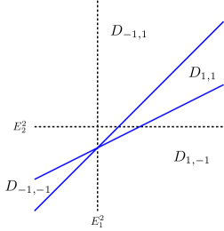
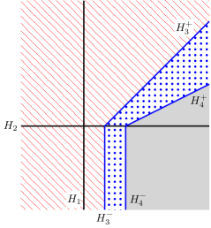
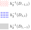
Figure 3: Left. The closed polyhedra of $\Pi_{2}$. Right. The reciprocal images by $h_{2}$ of the closed polyhedra of $\Pi_{2}$.

Let us now check the conditions one by one.

• The matrices $M^{2}$ and $M^{1}$ are both full row rank, so $\mathbf{P}.a)$ is satisfied for $k=2$ and $k=1$.

• Let us first show the condition for $k=2$. We have $\ring{\Omega}_{3}=\ring{\Omega}=\mathbb{R}^{2}$, so taking $x_{1}=(0,1)^{T}\in\ring{\Omega}_{3}$ and $x_{2}=(1,0)^{T}\in\ring{\Omega}_{3}$, we find

  $$\begin{cases}M^{2}_{1,.}x_{1}+b^{2}_{1}=\begin{pmatrix}1&0\end{pmatrix}\begin{pmatrix}0\\ 1\end{pmatrix}=0\\ M^{2}_{2,.}x_{2}+b^{2}_{2}=\begin{pmatrix}0&1\end{pmatrix}\begin{pmatrix}1\\ 0\end{pmatrix}=0.\end{cases}$$

  Let us now show the condition for $k=1$. We have $\ring{\Omega}_{k+1}=\ring{\Omega}_{2}=(\mathbb{R}_{+}^{*})^{2}$. Let us choose $x_{3}=(2,1)^{T}\in\ring{\Omega}_{2}$ and $x_{4}=(4,1)^{T}\in\ring{\Omega}_{2}$. We have

  $$\begin{cases}M^{1}_{1,.}x_{3}+b^{1}_{1}=\begin{pmatrix}1&-1\end{pmatrix}\begin{pmatrix}2\\ 1\end{pmatrix}-1=0\\ M^{1}_{2,.}x_{4}+b^{1}_{2}=\begin{pmatrix}-1&2\end{pmatrix}\begin{pmatrix}4\\ 1\end{pmatrix}+2=0.\end{cases}$$

  This shows that $\mathbf{P}.b)$ is satisfied for $k=2$ and $k=1$.

• For $k=2$, let us recall from (16) the values of $V^{2}(D)$ for all $D\in\Pi_{2}$. In the case of $V^{2}(D_{1,-1})$ and $V^{2}(D_{-1,1})$, $\mathbf{P}.c)$ is clearly satisfied. When it comes to $D_{1,1}$, we have $V^{2}_{.,1}(D_{1,1})=0$, but $D_{1,1}$ does not intersect $E^{2}_{1}$ in $\Omega_{2}$. Finally, we have $V^{2}_{.,1}(D_{-1,-1})=V^{2}_{.,2}(D_{-1,-1})=0$, but $D_{-1,-1}\cap\Omega_{2}=\emptyset$.

  We thus conclude that $\mathbf{P}.c)$ is satisfied for $k=2$.

  The case $k=1$ is easier, $\Pi_{1}=\{\mathbb{R}^{2}\}$ and for all $x\in\mathbb{R}^{2}$, we have $g_{1}(x)=M^{0}x+b^{0}$, so we have $V^{1}(\mathbb{R}^{2})=M^{0}=\begin{pmatrix}1&1\end{pmatrix}$, and $\mathbf{P}.c)$ is clearly satisfied.

• Here, the case $k=1$ is trivial since $\Pi_{1}=\{\mathbb{R}^{2}\}$, and $h_{1}^{-1}(\mathbb{R}^{2})=\mathbb{R}^{2}$, and thus $\partial h_{1}^{-1}(\mathbb{R}^{2})=\emptyset$.

  We thus only need to study the case $k=2$. Let us first determine the sets $h_{2}^{-1}(D)$, for $D\in\Pi_{2}$. We remind that for all $x\in\mathbb{R}^{2}$, $h_{2}(x)=\sigma(x)$.

  For this, let us divide $\mathbb{R}^{2}$ in $3$ regions. Let $x=(x_{1},x_{2})\in\mathbb{R}^{2}$.

  • If $x_{1}<0$, then $h_{2}(x)=(0,\sigma(x_{2}))^{T}$. We thus have

    $$M^{1}h_{2}(x)+b^{1}=\begin{pmatrix}-1(\sigma(x_{2})+1)\\ 2(\sigma(x_{2})+1)\end{pmatrix}.$$

    Since $\sigma(x_{2})\geq 0$, we see that $h_{2}(x)\in D_{-1,1}$.

  • If $x_{1}\geq 0$ and $x_{2}<0$, then $h_{2}(x)=(x_{1},0)^{T}$. We thus have

    $$M^{1}h_{2}(x)+b^{1}=\begin{pmatrix}x_{1}-1\\ -x_{1}+2\end{pmatrix}.$$

    There are $3$ possibilities: if $x_{1}\leq 1$, then $h_{2}(x)\in D_{-1,1}$, if $1\leq x_{1}\leq 2$, $h_{2}(x)\in D_{1,1}$, and if $2\leq x_{1}$, $h_{2}(x)\in D_{1,-1}$.

  • If $x_{1},x_{2}\geq 0$, then $h_{2}(x)=x$ and for all $D_{\epsilon_{1},\epsilon_{2}}\in\Pi_{2}$, $h_{2}(x)\in D_{\epsilon_{1},\epsilon_{2}}\Longleftrightarrow x\in D_{\epsilon_{1},\epsilon_{2}}$. There are $3$ possibilities, $x\in D_{-1,1},x\in D_{1,-1}$ and $x\in D_{1,1}$ since $D_{-1,-1}\cap(\mathbb{R}_{+})^{2}=\emptyset$.

  Summarizing, we find (see also Figure 3):

  $$h_{2}^{-1}(D_{-1,1})=\mathbb{R}_{-}\times\mathbb{R}\quad\cup\quad[0,1]\times\mathbb{R}_{-}\quad\cup\quad(\mathbb{R}_{+})^{2}\cap D_{-1,1}$$

  $$h_{2}^{-1}(D_{1,1})=[1,2]\times\mathbb{R}_{-}\quad\cup\quad(\mathbb{R}_{+})^{2}\cap D_{1,1}$$

  $$h_{2}^{-1}(D_{1,-1})=[2,+\infty[\times\mathbb{R}_{-}\quad\cup\quad(\mathbb{R}_{+})^{2}\cap D_{1,-1}$$

  $$h_{2}^{-1}(D_{-1,-1})=\emptyset.$$

  To express the boundaries of these regions, we define the following pieces of hyperplanes:

  $$H_{3}^{+}=\{x=(x_{1},x_{2})\in\mathbb{R}^{2},\quad x_{1}\geq 0,x_{2}\geq 0,M^{1}_{1,.}x+b^{1}_{1}=0\}$$

  $$H_{4}^{+}=\{x=(x_{1},x_{2})\in\mathbb{R}^{2},\quad x_{1}\geq 0,x_{2}\geq 0,M^{1}_{2,.}x+b^{1}_{2}=0\}$$

  $$H_{3}^{-}=\{x=(x_{1},x_{2})\in\mathbb{R}^{2},\quad x_{1}=1,x_{2}\leq 0\}$$

  $$H_{4}^{-}=\{x=(x_{1},x_{2})\in\mathbb{R}^{2},\quad x_{1}=2,x_{2}\leq 0\}.$$

  We have

  $$\partial h_{2}^{-1}(D_{-1,1})=H_{3}^{-}\cup H_{3}^{+}$$

  $$\partial h_{2}^{-1}(D_{1,1})=H_{3}^{-}\cup H_{3}^{+}\cup H_{4}^{-}\cup H_{4}^{+}$$

  $$\partial h_{2}^{-1}(D_{1,-1})=H_{4}^{-}\cup H_{4}^{+}$$

  $$\partial h_{2}^{-1}(D_{-1,-1})=\emptyset,$$

  and thus,

  $$\bigcup_{D\in\Pi_{2}}\partial h_{2}^{-1}(D)=H_{3}^{-}\cup H_{3}^{+}\cup H_{4}^{-}\cup H_{4}^{+}.$$ (17)

  Let us check the condition $\mathbf{P}.d)$ for $k=2$. Since $\Omega_{3}=\mathbb{R}^{2}$, here $\ring{\Omega}_{3}\cap H=H$. The condition is thus satisfied if and only if $\bigcup_{D\in\Pi_{2}}\partial h_{2}^{-1}(D)$ does not contain any full hyperplane $H$, and (17) shows that it is the case. The condition $\mathbf{P}.d)$ is satisfied.

Let us now discuss the conditions given in [47, 52] for this example. Let us first define the following hyperplanes:

$$H_{1}=\{x\in\mathbb{R}^{2},M^{2}_{1,.}x+b^{2}_{1}=0\}$$

$$H_{2}=\{x\in\mathbb{R}^{2},M^{2}_{2,.}x+b^{2}_{2}=0\}.$$

To discuss the conditions in [47], we will refer to their concepts of fold-set, of piece-wise linear surface, of canonical representation and dependency graph of a piece-wise linear surface, as well as to their Lemma 4. We also use their notations $\square_{1}S$ and $\square_{2}S$. Let us now consider the set $S$ as the fold-set of the function $f_{\mathbf{M},\mathbf{b}}$ implemented by the network. Here, it corresponds to the points $x$ satisfying one of the following equations

$$\begin{cases}M^{2}_{1,.}x+b^{2}_{1}=0\\ M^{2}_{2,.}x+b^{2}_{2}=0\\ M^{1}_{1,.}h_{2}(x)+b^{1}_{1}=0\\ M^{1}_{2,.}h_{2}(x)+b^{1}_{2}=0.\end{cases}$$

In other words, $S=H_{1}\cup H_{2}\cup H_{3}^{-}\cup H_{3}^{+}\cup H_{4}^{-}\cup H_{4}^{+}$. The canonical representation of $S$ is the following

$$S=\left(H_{1}\cup H_{2}\right)\cup\left(H_{3}^{-}\cup H_{3}^{+}\cup H_{4}^{-}\cup H_{4}^{+}\right),$$

where $\square_{1}S=\left(H_{1}\cup H_{2}\right)$ and $\square_{2}S=S$. Further, it can be checked that the dependency graph of $S$ only contains the edges: $H_{2}\rightarrow H_{3}^{-}$, $H_{2}\rightarrow H_{3}^{+}$, $H_{2}\rightarrow H_{4}^{-}$ and $H_{2}\rightarrow H_{4}^{+}$.

The identifiable networks considered in [47] must satisfy the conditions of Lemma 4 in [47]. In particular, the dependency graph of $S$ must contain at least $2$ directed paths of length $1$ with distinct starting vertices, which is not the case here since all the paths of length $1$ start from $H_{2}$. Hence, this network does not fall under the conditions of [47].

Now if we use the concepts and notations of [52], let us denote by $z_{1}$ the first neuron of the first hidden layer, whose associated parameters are $M^{2}_{1,.}$ and $b^{2}_{1}$. Following the definition in [52], the boundary associated to $z_{1}$ is $B_{z_{1}}=H_{1}$. Let us denote by $z_{3}$ the first neuron of the second hidden layer, whose associated parameters are $M^{1}_{1,.}$ and $b^{1}_{1}$. Its boundary is $B_{z_{3}}=H_{3}^{-}\cup H_{3}^{+}$. Since $z_{1}$ and $z_{3}$ belong to two consecutive layers and are thus linked by an edge of the network, the conditions in [52] (see Theorem 2) require that $B_{z_{1}}$ and $B_{z_{3}}$ intersect. It is however clear that they do not (see Figure 3).

5 Sketch of proof of Theorem 7

Our main result, Theorem 7, is proven in details in Appendix B.4, and we give a sketch of the proof in this section. It is proven by induction. We are given two parameterizations $\mathbf{(M,b)}$ and $\mathbf{(\tilde{M},\tilde{b})}$, two lists $\boldsymbol{\Pi}$ and $\boldsymbol{\tilde{\Pi}}$ that are admissible with respect to $\mathbf{(M,b)}$ and $\mathbf{(\tilde{M},\tilde{b})}$ respectively, and a domain $\Omega$ that satisfy the hypotheses of Theorem 7 and we want to show that the two parameterizations are equivalent. For this, we identify the layers one after the other. To facilitate identification at a layer level, we begin with a normalisation step.

5.1 Normalisation step

Two equivalent parameterizations do not necessarily have equal weights on their layers. Indeed, the neuron permutations but more importantly the rescalings can change the structure of the intermediate layers. We are going to assume the following normalisation property: for all $k\in\llbracket 1,K-1\rrbracket$, for all $i\in\llbracket 1,n_{k}\rrbracket$, we have

$$\|M^{k}_{i,.}\|=1;$$ (18)

$$\|\tilde{M}^{k}_{i,.}\|=1.$$

Indeed, we show in the appendix that for a parameterization satisfying the conditions $\mathbf{P}$, there always exists an equivalent parameterization that is normalised and that satisfies the conditions $\mathbf{P}$ (see Propositions 42 and 50). We can thus replace each parameterization $\mathbf{(M,b)}$ and $\mathbf{(\tilde{M},\tilde{b})}$ by an equivalent normalised parameterization. If we are able to show the normalised parameterizations are equivalent, then the original parameterizations are equivalent too.

5.2 Induction

The induction proof relies on Lemma 14 below. Let $K$ be the number of layers of the network, and suppose the theorem is true for the networks with $K-1$ layers. As explained in section 4.1, to identify the parameters $M^{K-1}$ and $b^{K-1}$, we separate the function implemented by the first layer of the network and the function implemented by the rest of the layers. For each network:

$$g_{K}=g_{K-1}\circ h_{K-1},$$

$$\tilde{g}_{K}=\tilde{g}_{K-1}\circ\tilde{h}_{K-1}.$$

We know that $g_{K-1}$ and $\tilde{g}_{K-1}$ are continuous piecewise linear, and this will allow us to apply Lemma 14. Before stating it, we introduce a set of conditions, called $\mathbf{C}$, that need to be satisfied in order to apply it. These conditions come immediately from $\mathbf{P}$, and one can easily check that $(g_{K-1},M^{K-1},b^{K-1},\Omega_{K},\Pi_{K-1})$ and $(\tilde{g}_{K-1},\tilde{M}^{K-1},\tilde{b}^{K-1},\Omega_{K},\tilde{\Pi}_{K-1})$ satisfy $\mathbf{C}$, as a direct consequence of the conditions $\mathbf{P}$ being satisfied by $\mathbf{(M,b,\Omega,\boldsymbol{\Pi})}$ and $\mathbf{(\tilde{M},\tilde{b},\Omega,\boldsymbol{\tilde{\Pi}})}$.

Definition 13.

Let $l,m,n$ be integers, $M\in\mathbb{R}^{m\times l}$, $b\in\mathbb{R}^{m}$, $\Omega\subset\mathbb{R}^{l}$ be an open domain, let $g:\mathbb{R}^{m}\rightarrow\mathbb{R}^{n}$ a continuous piecewise linear function, and let $\Pi$ be an admissible set of polyhedra with respect to $g$.

Let $D\in\Pi$. The function $g$ coincides with a linear function on $D$. Since the interior of $D$ is nonempty, we define $V(D)\in\mathbb{R}^{n\times m}$ and $c(D)\in\mathbb{R}^{n}$ as the unique couple satisfying, for all $x\in D$:

$$g(x)=V(D)x+c(D).$$

We denote $E_{i}=\{x\in\mathbb{R}^{m},x_{i}=0\}$.

We say that $(g,M,b,\Omega,\Pi)$ satisfies the conditions $\mathbf{C}$ iif

• $M$ is full row rank;

• for all $i\in\llbracket 1,m\rrbracket$, there exists $x\in\ring{\Omega}$ such that

  $$M_{i,.}x+b_{i}=0,$$

  or equivalently, if we denote by $h^{lin}$ the function $x\mapsto Mx+b$, then

  $$E_{i}\cap h^{lin}(\ring{\Omega})\neq\emptyset;$$

• for all $D\in\Pi$, for all $i\in\llbracket 1,m\rrbracket$, if $E_{i}\cap D\cap h(\Omega)\neq\emptyset$ then $V_{.,i}(D)\neq 0$;

• for any affine hyperplane $H\subset\mathbb{R}^{l}$,

  $$H\cap\ring{\Omega}\ \not\subset\bigcup_{D\in\Pi}\partial h^{-1}(D).$$

We can now state the lemma.

Lemma 14.

Let $l,m,n\in\mathbb{N}^{*}$. Suppose $g,\tilde{g}:\mathbb{R}^{m}\rightarrow\mathbb{R}^{n}$ are continuous piecewise linear functions, $\Omega\subset\mathbb{R}^{l}$ is a subset and let $M,\tilde{M}\in\mathbb{R}^{m\times l}$, $b,\tilde{b}\in\mathbb{R}^{m}$. Denote $h:x\mapsto\sigma(Mx+b)$ and $\tilde{h}:x\mapsto\sigma(\tilde{M}x+\tilde{b})$. Assume $\Pi$ and $\tilde{\Pi}$ are two sets of polyhedra admissible with respect to $g$ and $\tilde{g}$.

Suppose $(g,M,b,\Omega,\Pi)$ and $(\tilde{g},\tilde{M},\tilde{b},\Omega,\tilde{\Pi})$ satisfy the conditions $\mathbf{C}$, and for all $i\in\llbracket 1,m\rrbracket$, $\|M_{i,.}\|=\|\tilde{M}_{i,.}\|=1$.

Suppose for all $x\in\Omega$:

$$g\circ h(x)=\tilde{g}\circ\tilde{h}(x).$$

Then, there exists a permutation $\varphi\in\mathfrak{S}_{m}$, such that:

• $\tilde{M}=P_{\varphi}M$;

• $\tilde{b}=P_{\varphi}b$;

• $g$ and $y\mapsto\tilde{g}(P_{\varphi}y)$ coincide on ${h}(\Omega)$.

Lemma 14 is restated in Appendix B as Lemma 53 and proven in Appendix C.

Applying this lemma to $(g_{K-1},M^{K-1},b^{K-1},\Omega_{K},\Pi_{K-1})$ and $(\tilde{g}_{K-1},\tilde{M}^{K-1},\tilde{b}^{K-1},\Omega_{K},\tilde{\Pi}_{K-1})$, we conclude that there exists a permutation $\varphi_{K-1}$ such that

$$\begin{cases}\tilde{M}^{K-1}=P_{\varphi_{K-1}}M^{K-1}\\ \tilde{b}^{K-1}=P_{\varphi_{K-1}}b^{K-1},\end{cases}$$ (19)

and that $g_{K-1}$ and $y\mapsto\tilde{g}(P_{\varphi_{K-1}}y)$ coincide on $h_{K-1}(\Omega)$.

The functions $g_{K-1}$ and $y\mapsto\tilde{g}(P_{\varphi_{K-1}}y)$ are the functions implemented by the networks $\mathbf{(M,b)}$ and $\mathbf{(\tilde{M},\tilde{b})}$ once we have removed the first layer, with a permutation of the input for the second one. Since they coincide on $\Omega_{K-1}=h_{K-1}(\Omega)$ and they satisfy the conditions $\mathbf{P}$, we can apply the induction hypothesis to conclude the proof of Theorem 7. The complete proof is detailed in the appendices, as discussed above.

6 Conclusion

We established a set of conditions $\mathbf{P}$ under which the function implemented by a deep feedforward ReLU neural network on a subset $\Omega$ of the input space uniquely characterizes its parameters, up to permutation and positive rescaling. This contributes to the understanding of identifiability and stable recovery for deep ReLU networks, which is still largely unexplored. The conditions under which our result holds differ from the conditions of the results established in [47] and [52], which allows us to cover new situations. To be satisfied the conditions $\mathbf{P}$ need $\Omega$ to have nonempty interior, which prevents it from being a sample set. The authors of [59, 6] are able to give a result with a finite set $\Omega$, but for local identifiability only. Obtaining the best of both worlds, that is establishing a global identifiability result for deep ReLU networks with a finite set $\Omega$, would be a major step forward.

Appendix A Definitions, notations and preliminary results

Appendix A is structured as follows: after giving some notations in Section A.1, we recall the definition of a continuous piecewise linear function and some corresponding basic properties in Section A.2 and we give our formalization of deep ReLU networks as well as some well-known properties in Section A.3.

A.1 Basic notations and definitions

We denote by

$$\begin{array}[]{rrcl}\sigma:&\mathbb{R}&\longrightarrow&\mathbb{R}\\ &t&\longmapsto&\max(t,0)\end{array}$$

the ReLU activation function. If $x=(x_{1},\dots,x_{m})^{T}\in\mathbb{R}^{m}$ is a vector, we denote $\sigma(x)=(\sigma(x_{1}),\dots,\sigma(x_{m}))^{T}$.

If $A\subset\mathbb{R}^{m}$, we denote by $\ring{A}$ the interior of $A$ and $\overline{A}$ the closure of $A$ with respect to the standard topology of $\mathbb{R}^{m}$. We denote by $\partial A=\overline{A}\backslash\ring{A}$ the topological boundary of $A$.

For $m,n\in\mathbb{N}^{*}$, we denote by $\mathbb{R}^{n}$ the vector space of $n$-dimensional real vectors and $\mathbb{R}^{m\times n}$ the vector space of real matrices with $m$ lines and $n$ columns. On the space of vectors, we use the norm $\|x\|=\sqrt{\sum_{i=1}^{n}x_{i}^{2}}$. For $x\in\mathbb{R}^{n}$ and $r>0$, we denote $B(x,r)=\{y\in\mathbb{R}^{n},\|y-x\|<r\}$.

For any vector $x\in\mathbb{R}^{n}$ whose coefficients $x_{i}$ are all different from zero, we denote by $x^{-1}$ or $\frac{1}{x}$ the vector $\left(\frac{1}{x_{1}},\frac{1}{x_{2}},\dots,\frac{1}{x_{n}}\right)^{T}$.

For any matrix $M\in\mathbb{R}^{m\times n}$, for all $i\in\llbracket 1,m\rrbracket$, we denote by $M_{i,.}$ the $i^{\text{th}}$ line of $M$. The vector $M_{i,.}$ is a line vector whose $j^{\text{th}}$ component is $M_{i,j}$. Similarly, for $j\in\llbracket 1,n\rrbracket$, we denote by $M_{.,j}$ the $j^{\text{th}}$ column of $M$, which is the column vector whose $i^{\text{th}}$ component is $M_{i,j}$. For any matrix $M\in\mathbb{R}^{m\times n}$, we denote by $M^{T}\in\mathbb{R}^{n\times m}$ the transpose matrix of $M$.

To avoid any confusion, we will denote by $(M^{T})_{i,.}$ the $i^{\text{th}}$ line of the matrix $M^{T}$ and by $M_{i,.}^{\hskip 5.0ptT}$ the transpose of the line vector $M_{i,.}$, which is a column vector. Similarly, we will denote by $(M^{T})_{.,j}$ the $j^{\text{th}}$ column of $M^{T}$ and $M_{.,j}^{\hskip 5.0ptT}$ the transpose of the column vector $M_{.,j}$.

For $n\in\mathbb{N}^{*}$, we denote by $\operatorname{Id}_{n}$ the $n\times n$ identity matrix and by $\mathbf{1}_{n}$ the vector $(1,1,\dots,1)^{T}\in\mathbb{R}^{n}$.

If $\lambda\in\mathbb{R}^{n}$ is a vector of size $n$, for some $n\in\mathbb{N}^{*}$, we denote by $\operatorname{Diag}(\lambda)$ the $n\times n$ matrix defined by:

$$\operatorname{Diag}(\lambda)_{i,j}=\begin{cases}\lambda_{i}&\text{if }i=j\\ 0&\text{otherwise.}\end{cases}$$

For any integer $m\in\mathbb{N}^{*}$, we denote by $\mathfrak{S}_{m}$ the set of all permutations of $\llbracket 1,m\rrbracket$. We denote by $id_{\llbracket 1,m\rrbracket}$ and $id_{\mathbb{R}^{m}}$ the identity functions on $\llbracket 1,m\rrbracket$ and $\mathbb{R}^{m}$ respectively.

For any permutation $\varphi\in\mathfrak{S}_{m}$, we denote by $P_{\varphi}$ the $m\times m$ permutation matrix associated to $\varphi$:

$$\forall i,j\in\llbracket 1,m\rrbracket,\quad(P_{\varphi})_{i,j}=\begin{cases}1&\text{if }\varphi(j)=i\\ 0&\text{otherwise.}\end{cases}$$ (20)

For all $x\in\mathbb{R}^{m}$, we have:

$$(P_{\varphi}x)_{i}=x_{\varphi^{-1}(i)}.$$ (21)

Using (21) we see that $P_{\varphi^{-1}}P_{\varphi}x=x$, which shows, since $P_{\varphi}$ is orthogonal, that we have

$$P_{\varphi}^{-1}=P_{\varphi^{-1}}=P_{\varphi}^{T}.$$ (22)

Let $l,m,n\in\mathbb{N}^{*}$. For any matrix $M\in\mathbb{R}^{m\times l}$ and any function $f:\mathbb{R}^{m}\rightarrow\mathbb{R}^{n}$, we denote with a slight abuse of notation $f\circ M$ the function $x\mapsto f(Mx)$.

If $X$ and $Y$ are two sets and $h:X\rightarrow Y$ is a function, for a subset $A\subset Y$, we denote by $h^{-1}(A)$ the following set:

$$\{x\in X,h(x)\in A\}.$$

Note that this does not require the function $h$ to be injective.

A.2 Continuous piecewise linear functions

We now introduce a few definitions and properties around the notion of continuous piecewise linear function.

Definition 15.

Let $m\in\mathbb{N^{*}}$. A subset $D\subset\mathbb{R}^{m}$ is a closed polyhedron iif there exist $q\in\mathbb{N}^{*}$, $a_{1},\dots,a_{q}\in\mathbb{R}^{m}$ and $b_{1},\dots b_{q}\in\mathbb{R}$ such that for all $x\in\mathbb{R}^{m}$,

$$x\in D\quad\Longleftrightarrow\quad\begin{cases}a_{1}^{T}x+b_{1}\leq 0\\ \vdots\\ a_{q}^{T}x+b_{q}\leq 0.\end{cases}$$

Remarks.

• A closed polyhedron is convex as an intersection of convex sets.

• Since we can fuse the inequation systems of several closed polyhedrons into one system, we see that an intersection of closed polyhedrons is a closed polyhedron.

• For $q=1$ and $a_{1}=0$, taking $b_{1}>0$ and $b_{1}\leq 0$ respectively we can show that $\emptyset$ and $\mathbb{R}^{m}$ are both closed polyhedra.

Proposition 16.

Let $m,l\in\mathbb{N}^{*}$. If $h:\mathbb{R}^{l}\rightarrow\mathbb{R}^{m}$ is linear and $C$ is a closed polyhedron of $\mathbb{R}^{m}$, then $h^{-1}(C)$ is a closed polyhedron of $\mathbb{R}^{l}$.

Proof.

The function $h$ is linear so there exist $M\in\mathbb{R}^{m\times l}$ and $b\in\mathbb{R}^{m}$ such that for all $x\in\mathbb{R}^{l}$,

$$h(x)=Mx+b.$$

The set $C$ is a closed polyhedron so there exist $a_{1},\dots,a_{q}\in\mathbb{R}^{m}$ and $b_{1},\dots b_{q}\in\mathbb{R}$ such that $y\in C$ if and only if

$$\begin{cases}a_{1}^{T}y+b_{1}\leq 0\\ \vdots\\ a_{q}^{T}y+b_{q}\leq 0.\end{cases}$$

For all $x\in\mathbb{R}^{l}$,

$$x\in h^{-1}(C) \Longleftrightarrow\quad h(x)\in C$$

$$\Longleftrightarrow\quad\begin{cases}a_{1}^{T}(Mx+b)+b_{1}\leq 0\\ \vdots\\ a_{q}^{T}(Mx+b)+b_{q}\leq 0\end{cases}$$

$$\Longleftrightarrow\quad\begin{cases}(a_{1}^{T}M)x+(a_{1}^{T}b+b_{1})\leq 0\\ \vdots\\ (a_{q}^{T}M)x+(a_{q}^{T}b+b_{q})\leq 0.\end{cases}$$

This shows that $h^{-1}(C)$ is a closed polyhedron. ∎

Definition 17.

We say that a function $g:\mathbb{R}^{m}\rightarrow\mathbb{R}^{n}$ is continuous piecewise linear if there exists a finite set of closed polyhedra whose union is $\mathbb{R}^{m}$ and such that $g$ is linear over each polyhedron.

Example.

Since $\mathbb{R}^{m}$ is a closed polyhedron, we see in particular that an affine function $x\mapsto Ax+b$, with $A\in\mathbb{R}^{n\times m}$ and $b\in\mathbb{R}^{n}$, is continuous piecewise linear from $\mathbb{R}^{m}$ to $\mathbb{R}^{n}$.

Example 18.

The vectorial ReLU function $\sigma:\mathbb{R}^{m}\rightarrow\mathbb{R}^{m}$ is continuous piecewise linear. Indeed, each of the $2^{m}$ closed orthants is a closed polyhedron, defined by a system of the form

$$\begin{cases}\epsilon_{1}x_{1}\geq 0\\ \vdots\\ \epsilon_{m}x_{m}\geq 0,\end{cases}$$

with $\epsilon_{i}\in\{-1,1\}$, and over such an orthant, the ReLU coincides with the affine function

$$(x_{1},\dots,x_{m})\mapsto\left(\frac{1+\epsilon_{1}}{2}x_{1},\dots,\frac{1+\epsilon_{m}}{2}x_{m}\right).$$

In this definition the continuity is not obvious. We show it in the following proposition.

Proposition 19.

A continuous piecewise linear function is continuous.

Proof.

Let $g:\mathbb{R}^{m}\rightarrow\mathbb{R}^{n}$ be a continuous piecewise linear function. There exists a finite family of closed polyhedra $C_{1},\dots,C_{r}$ such that $\bigcup_{i=1}^{r}C_{i}=\mathbb{R}^{m}$ and $g$ is linear on each closed polyhedron $C_{i}$.

Let $x\in\mathbb{R}^{m}$. Let $\epsilon>0$.

Let us denote $I=\{i\in\llbracket 1,n\rrbracket,\ x\in C_{i}\}$. Since the polyhedrons are closed, there exists $r_{0}>0$ such that for all $i\notin I,B(x,r_{0})\cap C_{i}=\emptyset$. We thus have

$$B(x,r_{0})=\bigcup_{i=1}^{m}(B(x,r_{0})\cap C_{i})=\bigcup_{i\in I}\left(B(x,r_{0})\cap C_{i}\right).$$

For all $i\in I$, $g$ is linear -therefore continuous- on $C_{i}$ so there exists $r_{i}>0$, such that

$$y\in C_{i}\cap B(x,r_{i})\ \Rightarrow\ \|g(y)-g(x)\|\leq\epsilon.$$

Let $r=\min(r_{0},\min_{i\in I}(r_{i}))$. For all $y\in B(x,r)$ there exists $i\in I$ such that $y\in C_{i}$, and since $r\leq r_{i}$, we have

$$\|g(y)-g(x)\|\leq\epsilon.$$

Summarizing, for any $x\in\mathbb{R}^{n}$ and for any $\epsilon>0$, there exists $r>0$ such that

$$y\in B(x,r)\ \Rightarrow\ \|g(y)-g(x)\|\leq\epsilon.$$

This shows $g$ is continuous. ∎

Proposition 20.

If $h:\mathbb{R}^{l}\rightarrow\mathbb{R}^{m}$ and $g:\mathbb{R}^{m}\rightarrow\mathbb{R}^{n}$ are two continuous piecewise linear functions, then $g\circ h$ is continuous piecewise linear.

Proof.

By definition there exist a family $C_{1},\dots,C_{r}$ of closed polyhedra of $\mathbb{R}^{l}$ such that $\bigcup_{i=1}^{r}C_{i}=\mathbb{R}^{l}$ and $h$ is linear on each $C_{i}$ and a family $D_{1},\dots,D_{s}$ of closed polyhedra of $\mathbb{R}^{m}$ such that $\bigcup_{i=1}^{s}D_{i}=\mathbb{R}^{m}$ and $g$ is linear on each $D_{i}$. Let $i\in\llbracket 1,r\rrbracket$ and $j\in\llbracket 1,s\rrbracket$. The function $h$ coincides with a linear map $\tilde{h}:\mathbb{R}^{l}\rightarrow\mathbb{R}^{m}$ on $C_{i}$ and the inverse image of a closed polyhedron by a linear map is a closed polyhedron (Proposition 16) so $\tilde{h}^{-1}(D_{j})$ is a closed polyhedron. Thus $h^{-1}(D_{j})\cap C_{i}=\tilde{h}^{-1}(D_{j})\cap C_{i}$ is a closed polyhedron as an intersection of closed polyhedra. The function $h$ is linear on $C_{i}$ and $g$ is linear on $D_{j}$ so $g\circ h$ is linear on $h^{-1}(D_{j})\cap C_{i}$. We have a family of closed polyhedra,

$$\left(h^{-1}(D_{j})\cap C_{i}\right)_{\begin{subarray}{c}i\in\llbracket 1,r\rrbracket\\ j\in\llbracket 1,s\rrbracket\end{subarray}},$$

each of which $g\circ h$ is linear over. Given that

$$\bigcup_{i=1}^{r}\bigcup_{j=1}^{s}h^{-1}(D_{j})\cap C_{i}=\bigcup_{i=1}^{r}C_{i}=\mathbb{R}^{l},$$

we can conclude that $g\circ h$ is continuous piecewise linear. ∎

Definition 21.

Let $g:\mathbb{R}^{m}\rightarrow\mathbb{R}^{n}$ be a continuous piecewise linear function. Let $\Pi$ be a set of closed polyhedra of $\mathbb{R}^{m}$. We say that $\Pi$ is admissible with respect to the function $g$ if and only if:

• $\bigcup_{D\in\Pi}D=\mathbb{R}^{m}$,

• for all $D\in\Pi$, $g$ is linear on $D$,

• for all $D\in\Pi$, $\ring{D}\neq\emptyset$.

Proposition 22.

For all $g:\mathbb{R}^{m}\rightarrow\mathbb{R}^{n}$ continuous piecewise linear, there exists a set of closed polyhedra $\Pi$ admissible with respect to $g$.

Proof.

Let $g:\mathbb{R}^{m}\rightarrow\mathbb{R}^{n}$ be a continuous piecewise linear function. By definition there exists a finite set of closed polyhedra $D_{1},\dots,D_{s}$ such that $\bigcup_{i=1}^{s}D_{i}=\mathbb{R}^{m}$ and $g$ is linear on each $D_{i}$.

Let $I=\{i\in\llbracket 1,s\rrbracket,\ring{D_{i}}\neq\emptyset\}$. Let us show that $\bigcup_{i\in I}D_{i}=\mathbb{R}^{m}$.

We first show that if a polyhedron $D_{i}$ has empty interior, then it is contained in an affine hyperplane. Indeed, if it is not contained in an affine hyperplane, then there exist $m+1$ affinely independent points $x_{1},\dots,x_{m+1}\in D_{i}$. Since a closed polyhedron is convex, the convex hull of the points $\operatorname{Conv}(x_{1},\dots,x_{m+1})$, which is a $m$-simplex, is contained in $D_{i}$, and thus $D_{i}$ has nonempty interior.

Let $x\in\mathbb{R}^{m}$. For all $i\notin I$, $D_{i}$ is contained in an affine hyperplane, and a finite union of affine hyperplanes does not contain any nontrivial ball. As a consequence, for all $n\in\mathbb{N}$, the ball $B(x,\frac{1}{n})$ is not contained in $\bigcup_{i\notin I}D_{i}$ and thus there exists $i_{n}\in I$ such that $D_{i_{n}}\cap B(x,\frac{1}{n})\neq\emptyset$. Since $I$ is finite, there exists $i\in I$ such that $i_{n}=i$ for infinitely many $n$, and thus $x\in\overline{D_{i}}$.

We have shown that for all $x\in\mathbb{R}^{m}$ there exists $i\in I$ such that $x\in\overline{D_{i}}=D_{i}$, which means that

$$\bigcup_{i\in I}D_{i}=\mathbb{R}^{m}.$$

Hence, the set $\Pi:=\{D_{i},i\in I\}$ is admissible with respect to $g$. ∎

Proposition 23.

Let $h:\mathbb{R}^{l}\rightarrow\mathbb{R}^{m}$ be a continuous piecewise linear function and let $\mathcal{P}$ be a finite set of closed polyhedra of $\mathbb{R}^{m}$. Then

• for all $D\in\mathcal{P}$, $h^{-1}(D)$ is a finite union of closed polyhedra;

• $\bigcup_{D\in\mathcal{P}}\partial h^{-1}(D)$ is contained in a finite union of hyperplanes $\bigcup_{k=1}^{s}A_{k}$.

Proof.

Consider $\Pi$ an admissible set of closed polyhedra with respect to $h$. Let $D\in\mathcal{P}$. Since $\bigcup_{C\in\Pi}C=\mathbb{R}^{l}$, we can write

$$h^{-1}(D)=h^{-1}(D)\cap\left(\bigcup_{C\in\Pi}C\right)=\bigcup_{C\in\Pi}\left(h^{-1}(D)\cap C\right).$$

For all $C\in\Pi$, $h$ is linear over $C$, so $h^{-1}(D)\cap C$ is a polyhedron (see Proposition 16). This shows the first point of the proposition.

Since $h^{-1}(D)\cap C$ is a polyhedron, $\partial\left(h^{-1}(D)\cap C\right)$ is contained in a finite union of hyperplanes. In topology, we have

$$\partial\left[\bigcup_{C\in\Pi}\left(h^{-1}(D)\cap C\right)\right]\ \subset\ \bigcup_{C\in\Pi}\partial\left(h^{-1}(D)\cap C\right),$$

which shows that $\partial\left[\bigcup_{C\in\Pi}\left(h^{-1}(D)\cap C\right)\right]$ i.e. $\partial h^{-1}(D)$ is contained in a finite union of hyperplanes too. This is true for any $D\in\mathcal{P}$, and since $\mathcal{P}$ is finite, this is also true of the union $\bigcup_{D\in\mathcal{P}}\partial h^{-1}(D)$. ∎

A.3 Neural networks

We consider fully connected feedforward neural networks, with ReLU activation function. We index the layers in reverse order, from $K$ to $0$, for some $K\geq 2$. The input layer is the layer $K$, the output layer is the layer $0$, and between them are $K-1$ hidden layers. For $k\in\llbracket 0,K\rrbracket$, we denote by $n_{k}\in\mathbb{N}$ the number of neurons of the layer $k$. This means the information contained at the layer $k$ is a $n_{k}$-dimensional vector.

Let $k\in\llbracket 0,K-1\rrbracket$. We denote the weights between the layer $k+1$ and the layer $k$ with a matrix $M^{k}\in\mathbb{R}^{n_{k}\times n_{k+1}}$, and we consider a bias $b^{k}\in\mathbb{R}^{n_{k}}$ in the layer $k$. If $k\neq 0$, we add a ReLU activation function. If $x\in\mathbb{R}^{n_{k+1}}$ is the information contained at the layer $k+1$, the layer $k$ contains:

$$\begin{cases}\sigma(M^{k}x+b^{k})&\text{if }k\neq 0\\ M^{0}x+b^{0}&\text{if }k=0.\end{cases}$$

The parameters of the network can be summarized in the couple $(\mathbf{M},\mathbf{b})$, where $\mathbf{M}=(M^{0},M^{1},\dots,M^{K-1})\in\mathbb{R}^{n_{0}\times n_{1}}\times\dots\times\mathbb{R}^{n_{K-1}\times n_{K}}$ and $\mathbf{b}=(b^{0},b^{1},\dots,b^{K-1})\in\mathbb{R}^{n_{0}}\times\dots\times\mathbb{R}^{n_{K-1}}$. We formalize the transformation implemented by one layer of the network with the following definition.

Definition 24.

For a network with parameters $(\mathbf{M},\mathbf{b})$, we define the family of functions $(h_{0},\dots,h_{K-1})$ such that for all $k\in\llbracket 0,K-1\rrbracket$, $h_{k}:\mathbb{R}^{n_{k+1}}\rightarrow\mathbb{R}^{n_{k}}$ and for all $x\in\mathbb{R}^{n_{k}}$,

$$h_{k}(x)=\begin{cases}\sigma(M^{k}x+b^{k})&\text{if }k\neq 0\\ M^{0}x+b^{0}&\text{if }k=0.\end{cases}$$

The function implemented by the network is then

$$f_{\mathbf{M},\mathbf{b}}=h_{0}\circ h_{1}\circ\dots\circ h_{K-1}:\mathbb{R}^{n_{K}}\longrightarrow\mathbb{R}^{n_{0}}.$$ (23)

The network with its parameters are represented in Figure 1 in the main part.

For all $l\in\llbracket 0,K-1\rrbracket$, we denote $\mathbf{M}^{\leq l}=(M^{0},M^{1},\dots,M^{l})$ and $\mathbf{b}^{\leq l}=(b^{0},b^{1},\dots,b^{l})$.

Remark 25.

Since the vectorial ReLU function is continuous piecewise linear, Proposition 20 guarantees that the functions $h_{k}$ are continuous piecewise linear.

We now define a few more functions associated to a network.

Definition 26.

For a network with parameters $(\mathbf{M},\mathbf{b})$, we define the family of functions $(h^{lin}_{0},\dots,h^{lin}_{K-1})$ such that for all $k\in\llbracket 0,K-1\rrbracket$, $h_{k}^{lin}:\mathbb{R}^{n_{k+1}}\rightarrow\mathbb{R}^{n_{k}}$ and for all $x\in\mathbb{R}^{n_{k+1}}$,

$$h_{k}^{lin}(x)=M^{k}x+b^{k}.$$

The functions $h_{k}^{lin}$ correspond to the linear part of the transformation implemented by the network between two layers, before applying the activation $\sigma$.

Definition 27.

For a network with parameters $(\mathbf{M},\mathbf{b})$, we define the family of functions $(f_{K},f_{K-1},\dots,f_{0})$ as follows:

• $f_{K}=id_{\mathbb{R}^{n_{K}}}$,

• for all $k\in\llbracket 0,K-1\rrbracket$,  $f_{k}=h_{k}\circ h_{k+1}\circ\dots\circ h_{K-1}$.

Remark.

In particular we have $f_{0}=f_{\mathbf{M},\mathbf{b}}$.

The function $f_{k}:\mathbb{R}^{n_{K}}\mapsto\mathbb{R}^{n_{k}}$ represents the transformation implemented by the network between the input layer and the layer $k$.

Definition 28.

For a network with parameters $(\mathbf{M},\mathbf{b})$, we define the sequence $(g_{0},\dots,g_{K})$ as follows:

• $g_{0}=id_{\mathbb{R}^{n_{0}}}$,

• for all $k\in\llbracket 1,K\rrbracket$,  $g_{k}=h_{0}\circ h_{1}\circ\dots\circ h_{k-1}$.

Remark.

We have in particular

• $g_{K}=f_{\mathbf{M,b}}$;

• for all $k\in\llbracket 0,K\rrbracket$, $f_{\mathbf{M},\mathbf{b}}=g_{k}\circ f_{k}$.

The function $g_{k}:\mathbb{R}^{n_{k}}\mapsto\mathbb{R}^{n_{0}}$ represents the transformation implemented by the network between the layer $k$ and the output layer.

In this paper the functions implemented by the networks are considered on a subset $\Omega\subset\mathbb{R}^{n_{K}}$. The successive layers of a network project this subset onto the spaces $\mathbb{R}^{n_{k}}$, inducing a subset $\Omega_{k}$ of $\mathbb{R}^{n_{k}}$ for all $k$, as in the following definition.

Definition 29.

For a network with parameters $(\mathbf{M},\mathbf{b})$, for any $\Omega\subset\mathbb{R}^{n_{K}}$, we denote for all $k\in\llbracket 0,K\rrbracket$,

$$\Omega_{k}=f_{k}(\Omega).$$

Definition 30.

For a network with parameters $(\mathbf{M},\mathbf{b})$, for all $k\in\llbracket 2,K\rrbracket$, for all $i\in\llbracket 1,n_{k-1}\rrbracket$, we define

$$H_{i}^{k}=\{x\in\mathbb{R}^{n_{k}},\ M^{k-1}_{i,.}x+b_{i}^{k-1}=0\}.$$

Remark.

When $M^{k-1}_{i,.}\neq 0$, the set $H^{k}_{i}$ is a hyperplane.

Remark 31.

The objects defined in Definitions 24, 26, 27, 28, 29 and 30 all depend on $(\mathbf{M},\mathbf{b})$, but to simplify the notation we do not write it explicitly. To disambiguate when manipulating a second network, whose parameters we will denote by $(\mathbf{\tilde{M}},\mathbf{\tilde{b}})$, we will denote by $\tilde{h}_{k}$, $\tilde{h}_{k}^{lin}$, $\tilde{f}_{k}$, $\tilde{g}_{k}$, $\tilde{\Omega}_{k}$ and $\tilde{H}^{k}_{i}$ the corresponding objects.

Proposition 32.

For all $k\in\llbracket 0,K\rrbracket$, $f_{k}$ and $g_{k}$ are continuous piecewise linear.

Proof.

We show this by induction: for the initialisation we have $f_{K}=id_{\mathbb{R}^{n_{K}}}$ which is continuous piecewise linear. Now let $k\in\llbracket 0,K-1\rrbracket$ and assume $f_{k+1}$ is continuous piecewise linear. By definition, we have $f_{k}=h_{k}\circ f_{k+1}$. The function $h_{k}$ is continuous piecewise linear as noted in Remark 25. By Proposition 20, the composition of two continuous piecewise linear functions is continuous piecewise linear, so $f_{k}$ is continuous piecewise linear. The conclusion follows by induction.

We do the same for $(g_{0},\dots,g_{K})$ starting with $g_{0}$: first we have $g_{0}=id_{\mathbb{R}^{n_{0}}}$ which is continuous piecewise linear, then for all $k\in\llbracket 1,K\rrbracket$, we have $g_{k}=g_{k-1}\circ h_{k-1}$, and we conclude by composition of two continuous piecewise linear functions. ∎

Corollary 33.

The function $f_{\mathbf{M},\mathbf{b}}$ is continuous piecewise linear.

Proof.

It comes immediately from $f_{\mathbf{M},\mathbf{b}}=f_{0}$ and Proposition 32. ∎

Recall the definition of an admissible set with respect to a continuous piecewise linear function (Definition 21). Proposition 32 allows the following definition.

Definition 34.

Consider a network parameterization $\mathbf{(M,b)}$, and the functions $g_{k}$ associated to it. We say that a list of sets of closed polyhedra $\boldsymbol{\Pi}=(\Pi_{1},\dots,\Pi_{K-1})$ is admissible with respect to $(\mathbf{M},\mathbf{b})$ iif for all $k\in\llbracket 1,K-1\rrbracket$, the set $\Pi_{k}$ is admissible with respect to $g_{k}$.

Remark.

For a list $\boldsymbol{\Pi}=(\Pi_{1},\dots,\Pi_{K-1})$, for all $l\in\llbracket 1,K-1\rrbracket$, we denote $\boldsymbol{\Pi}^{\leq l}=(\Pi_{1},\dots,\Pi_{l})$. If $\boldsymbol{\Pi}$ is admissible with respect to $\mathbf{(M,b)}$, then $\boldsymbol{\Pi}^{\leq l}$ is admissible with respect to $(\mathbf{M}^{\leq l},\mathbf{b}^{\leq l})$.

Proposition 35.

For any network parameterization $\mathbf{(M,b)}$, there always exists a list of sets of closed polyhedra $\boldsymbol{\Pi}$ that is admissible with respect to $\mathbf{(M,b)}$.

Proof.

For all $k\in\llbracket 1,K-1\rrbracket$, since $g_{k}$ is continuous piecewise linear, Proposition 22 guarantees that there exists an admissible set of polyhedra $\Pi_{k}$ with respect to $g_{k}$. We simply define $\boldsymbol{\Pi}=(\Pi_{1},\dots,\Pi_{K-1})$. ∎

Definition 36.

For a parameterization $\mathbf{(M,b)}$ and a list $\boldsymbol{\Pi}$ admissible with respect to $\mathbf{(M,b)}$, for all $k\in\llbracket 1,K-1\rrbracket$, for all $D\in\Pi_{k}$, since $g_{k}$ is linear over $D$ and $D$ has nonempty interior, we can define $V^{k}(D)\in\mathbb{R}^{n_{0}\times n_{k}}$ and $c^{k}(D)\in\mathbb{R}^{n_{0}}$ as the unique couple that satisfies:

$$\forall x\in D,\quad g_{k}(x)=V^{k}(D)x+c^{k}(D).$$

We now introduce the equivalence relation between parameterizations, often referred to as equivalence modulo permutation and positive rescaling.

Definition 37 (Equivalent parameterizations).

If $(\mathbf{M},\mathbf{b})$ and $(\mathbf{\tilde{M}},\mathbf{\tilde{b}})$ are two network parameterizations, we say that $(\mathbf{M},\mathbf{b})$ is equivalent modulo permutation and positive rescaling, or simply equivalent, to $(\mathbf{\tilde{M}},\mathbf{\tilde{b}})$, and we write $(\mathbf{M},\mathbf{b})\sim(\mathbf{\tilde{M}},\mathbf{\tilde{b}})$, if and only if there exist:

• a family of permutations $\boldsymbol{\varphi}=(\varphi_{0},\dots,\varphi_{K})\in\mathfrak{S}_{n_{0}}\times\dots\times\mathfrak{S}_{n_{K}}$, with $\varphi_{0}=id_{\llbracket 1,n_{0}\rrbracket}$ and $\varphi_{K}=id_{\llbracket 1,n_{K}\rrbracket}$,

• a family of vectors $\boldsymbol{\lambda}=(\lambda^{0},\lambda^{1},\dots,\lambda^{K})\in(\mathbb{R_{+}^{*}})^{n_{0}}\times\dots\times(\mathbb{R_{+}^{*}})^{n_{K}}$, with $\lambda^{0}=\mathbf{1}_{n_{0}}$ and $\lambda^{K}=\mathbf{1}_{n_{K}}$,

such that for all $k\in\llbracket 0,K-1\rrbracket$,

$$\begin{cases}\tilde{M}^{k}=P_{\varphi_{k}}\operatorname{Diag}(\lambda^{k})M^{k}\operatorname{Diag}(\lambda^{k+1})^{-1}P_{\varphi_{k+1}}^{-1}\\ \tilde{b}^{k}=P_{\varphi_{k}}\operatorname{Diag}(\lambda^{k})b^{k}.\end{cases}$$ (24)

Remarks.

1. 
   

2. Recall that we denote by $\frac{1}{\lambda^{k+1}}$ the vector whose components are $\frac{1}{\lambda^{k+1}_{i}}$. Note that $\operatorname{Diag}(\lambda^{k+1})^{-1}=\operatorname{Diag}(\frac{1}{\lambda^{k+1}})$. Using (21), for all $k\in\llbracket 0,K-1\rrbracket$, (24) means that for all $(i,j)\in\llbracket 1,n_{k}\rrbracket\times\llbracket 1,n_{k+1}\rrbracket$,

   $$\tilde{M}^{k}_{i,j}=\frac{\lambda^{k}_{\varphi_{k}^{-1}(i)}}{\lambda^{k+1}_{\varphi_{k+1}^{-1}(j)}}M^{k}_{\varphi_{k}^{-1}(i),\varphi_{k+1}^{-1}(j)}$$

   and

   $$\tilde{b}^{k}_{i}=\lambda^{k}_{\varphi_{k}^{-1}(i)}b^{k}_{\varphi_{k}^{-1}(i)}.$$

3. We go from a parameterization to an equivalent one by:

   • permuting the neurons of each hidden layer $k$ with a permutation $\varphi_{k}$;

   • for each hidden layer $k$, multiplying all the weights of the edges arriving (from the layer $k+1$) to the neuron $j$, as well as the bias $b^{k}_{j}$, by some positive number $\lambda^{k}_{j}$, and multiplying all the weights of the edges leaving (towards the layer $k-1$) the neuron $j$ by $\frac{1}{\lambda^{k}_{j}}$.

Proposition 38.

The relation $\sim$ is an equivalence relation.

Proof.

Let us first show the following equality, that we are going to use in the proof. For any $n\in\mathbb{N}^{*}$, $\lambda\in\mathbb{R}^{n}$ and $\varphi\in\mathfrak{S}_{n}$,

$$\operatorname{Diag}(\lambda)P_{\varphi}=P_{\varphi}\operatorname{Diag}(P_{\varphi}^{-1}\lambda).$$ (25)

Indeed, $\operatorname{Diag}(\lambda)P_{\varphi}$ is the matrix obtained by multiplying each line $i$ of $P_{\varphi}$ by $\lambda_{i}$, so recalling (20), for all $i,j\in\llbracket 1,m\rrbracket$, we have

$$(\operatorname{Diag}(\lambda)P_{\varphi})_{i,j}=\begin{cases}\lambda_{i}&\text{if }\varphi(j)=i\\ 0&\text{otherwise.}\end{cases}$$

At the same time, $P_{\varphi}\operatorname{Diag}(P_{\varphi}^{-1}\lambda)$ is the matrix obtained by multiplying each column $j$ of $P_{\varphi}$ by $(P_{\varphi}^{-1}\lambda)_{j}=\lambda_{\varphi(j)}$ (see (21) and (22)), so for all $i,j\in\llbracket 1,m\rrbracket$, we have

$$(P_{\varphi}\operatorname{Diag}(P_{\varphi}^{-1}\lambda))_{i,j}=\begin{cases}\lambda_{\varphi(j)}&\text{if }\varphi(j)=i\\ 0&\text{otherwise.}\end{cases}$$

The two matrices are clearly equal.

We can now show the proposition.

• To show reflexivity we can take $\lambda^{k}=\mathbf{1}_{n_{k}}$ and $\varphi_{k}=id_{\llbracket 1,n_{k}\rrbracket}$ for all $k\in\llbracket 0,K\rrbracket$.

• Let us show symmetry. Assume a parameterization $\mathbf{(M,b)}$ is equivalent to another parameterization $\mathbf{(\tilde{M},\tilde{b})}$. Let us denote by $\boldsymbol{\varphi}$ and $\boldsymbol{\lambda}$ the corresponding families of permutations and vectors, as in Definition 37. Inverting the expression of $\tilde{M}^{k}$ in Definition 37 and using (25) twice, we have for all $k\in\llbracket 0,K-1\rrbracket$:

  $$\tilde{M}^{k}=P_{\varphi_{k}}\operatorname{Diag}(\lambda^{k})M^{k}\operatorname{Diag}(\lambda^{k+1})^{-1}P_{\varphi_{k+1}}^{-1}$$

  $$\Longleftrightarrow \operatorname{Diag}(\lambda^{k})^{-1}P_{\varphi_{k}}^{-1}\tilde{M}^{k}P_{\varphi_{k+1}}\operatorname{Diag}(\lambda^{k+1})=M^{k}$$

  $$\Longleftrightarrow P_{\varphi_{k}}^{-1}\operatorname{Diag}(P_{\varphi_{k}}\lambda^{k})^{-1}\tilde{M}^{k}\operatorname{Diag}(P_{\varphi_{k+1}}\lambda^{k+1})P_{\varphi_{k+1}}=M^{k},$$

  so denoting $\tilde{\varphi}_{k}=\varphi_{k}^{-1}$ and $\tilde{\lambda}^{k}=(P_{\varphi_{k}}\lambda^{k})^{-1}$, and recalling that $P_{\varphi_{k}^{-1}}=P_{\varphi_{k}}^{-1}$, we have, for all $k\in\llbracket 0,K-1\rrbracket$,

  $$M^{k}=P_{\tilde{\varphi}_{k}}\operatorname{Diag}(\tilde{\lambda}^{k})\tilde{M}^{k}\operatorname{Diag}(\tilde{\lambda}^{k+1})^{-1}P_{\tilde{\varphi}_{k+1}}^{-1}.$$

  We show similarly that for all $k\in\llbracket 0,K-1\rrbracket$,

  $$b^{k}=P_{\tilde{\varphi}_{k}}\operatorname{Diag}(\tilde{\lambda}_{k})\tilde{b}^{k}.$$

  We naturally have $\tilde{\varphi}_{0}=id_{\llbracket 1,n_{0}\rrbracket}$ and $\tilde{\varphi}_{K}=id_{\llbracket 1,n_{K}\rrbracket}$, as well as $\tilde{\lambda}^{0}=\mathbf{1}_{n_{0}}$ and $\tilde{\lambda}^{K}=\mathbf{1}_{n_{K}}$.

  This proves the symmetry of the relation.

• Let us show transitivity. Assume $\mathbf{(M,b)}$, $\mathbf{(\tilde{M},\tilde{b})}$ and $\mathbf{(\check{M},\check{b})}$ are three parameterizations such that $\mathbf{(M,b)}\sim\mathbf{(\tilde{M},\tilde{b})}$ and $\mathbf{(\tilde{M},\tilde{b})}\sim\mathbf{(\check{M},\check{b})}$.

  As in Definition 37, we denote by $\boldsymbol{\varphi}$, $\tilde{\boldsymbol{\varphi}}$, $\boldsymbol{\lambda}$ and $\tilde{\boldsymbol{\lambda}}$ the families of permutations and vectors such that, for all $k\in\llbracket 0,K-1\rrbracket$,

  $$\begin{cases}\tilde{M}^{k}=P_{\varphi_{k}}\operatorname{Diag}(\lambda^{k})M^{k}\operatorname{Diag}(\lambda^{k+1})^{-1}P_{\varphi_{k+1}}^{-1}\\ \tilde{b}^{k}=P_{{\varphi}_{k}}\operatorname{Diag}({\lambda}^{k})b^{k},\end{cases}$$

  and

  $$\begin{cases}\check{M}^{k}=P_{\tilde{\varphi}_{k}}\operatorname{Diag}(\tilde{\lambda}^{k})\tilde{M}^{k}\operatorname{Diag}(\tilde{\lambda}^{k+1})^{-1}P_{\tilde{\varphi}_{k+1}}^{-1}\\ \check{b}^{k}=P_{\tilde{\varphi}_{k}}\operatorname{Diag}(\tilde{\lambda}^{k})\tilde{b}^{k}.\end{cases}$$

  Combining these and using (25), we have

  $$\check{M}^{k} =P_{\tilde{\varphi}_{k}}\operatorname{Diag}(\tilde{\lambda}^{k})P_{\varphi_{k}}\operatorname{Diag}(\lambda^{k})M^{k}\operatorname{Diag}(\lambda^{k+1})^{-1}P_{\varphi_{k+1}}^{-1}\operatorname{Diag}(\tilde{\lambda}^{k+1})^{-1}P_{\tilde{\varphi}_{k+1}}^{-1}$$

  $$=P_{\tilde{\varphi}_{k}}\left(\operatorname{Diag}(\tilde{\lambda}^{k})P_{\varphi_{k}}\right)\operatorname{Diag}(\lambda^{k})M^{k}$$

  $$\hskip 90.0pt\cdot\operatorname{Diag}(\lambda^{k+1})^{-1}\left(\operatorname{Diag}(\tilde{\lambda}^{k+1})P_{\varphi_{k+1}}\right)^{-1}P_{\tilde{\varphi}_{k+1}}^{-1}$$

  $$=P_{\tilde{\varphi}_{k}}\left(P_{\varphi_{k}}\operatorname{Diag}(P_{\varphi_{k}}^{-1}\tilde{\lambda}^{k})\right)\operatorname{Diag}(\lambda^{k})M^{k}$$

  $$\hskip 90.0pt\cdot\operatorname{Diag}(\lambda^{k+1})^{-1}\left(P_{\varphi_{k+1}}\operatorname{Diag}(P_{\varphi_{k+1}}^{-1}\tilde{\lambda}^{k+1})\right)^{-1}P_{\tilde{\varphi}_{k+1}}^{-1}$$

  $$=P_{\tilde{\varphi}_{k}}P_{\varphi_{k}}\operatorname{Diag}(P_{\varphi_{k}}^{-1}\tilde{\lambda}^{k})\operatorname{Diag}(\lambda^{k})M^{k}$$

  $$\hskip 90.0pt\cdot\operatorname{Diag}(\lambda^{k+1})^{-1}\operatorname{Diag}(P_{\varphi_{k+1}}^{-1}\tilde{\lambda}^{k+1})^{-1}P_{\varphi_{k+1}}^{-1}P_{\tilde{\varphi}_{k+1}}^{-1},$$

  and

  $$\check{b}^{k} =P_{\tilde{\varphi}_{k}}\operatorname{Diag}(\tilde{\lambda}^{k})P_{\varphi_{k}}\operatorname{Diag}(\lambda^{k})b^{k}$$

  $$=P_{\tilde{\varphi}_{k}}P_{\varphi_{k}}\operatorname{Diag}(P_{\varphi_{k}}^{-1}\tilde{\lambda}^{k})\operatorname{Diag}(\lambda^{k})b^{k}.$$

  Hence denoting $\check{\varphi}_{k}=\tilde{\varphi}_{k}\circ\varphi_{k}$ and $\check{\lambda}^{k}=\operatorname{Diag}(P_{\varphi_{k}}^{-1}\tilde{\lambda}^{k})\lambda^{k}$, for all $k\in\llbracket 0,K\rrbracket$, we see that, for $k\in\llbracket 0,K-1\rrbracket$,

  $$\check{M}^{k}=P_{\check{\varphi}_{k}}\operatorname{Diag}(\check{\lambda}^{k})M^{k}\operatorname{Diag}(\check{\lambda}^{k+1})^{-1}P_{\check{\varphi}_{k+1}}^{-1}$$

  and

  $$\check{b}^{k}=P_{\check{\varphi}_{k}}\operatorname{Diag}(\check{\lambda}^{k})b^{k}.$$

  Naturally, we also have $\check{\varphi}_{0}=id_{\llbracket 1,n_{0}\rrbracket}$ and $\check{\varphi}_{K}=id_{\llbracket 1,n_{K}\rrbracket}$, as well as $\check{\lambda}^{0}=\mathbf{1}_{n_{0}}$ and $\check{\lambda}^{K}=\mathbf{1}_{n_{K}}$, which shows that $\mathbf{(M,b)}\sim\mathbf{(\check{M},\check{b})}$.

∎

Recall the objects $h_{k},f_{k},g_{k},\Omega_{k},H_{i}^{k}$ associated to a parameterization $(\mathbf{M},\mathbf{b})$, defined in Definitions 24, 27, 28, 29 and 30, and recall that we denote by $\tilde{h}_{k},\tilde{f}_{k},\tilde{g}_{k},\tilde{\Omega}_{k}$ and $\tilde{H}_{i}^{k}$ the corresponding objects with respect to another parameterization $\mathbf{(\tilde{M},\tilde{b})}$. We give in the following proposition the relations that link these objects when the two parameterizations $\mathbf{(M,b)}$ and $\mathbf{(\tilde{M},\tilde{b})}$ are equivalent.

Proposition 39.

Assume $(\mathbf{M},\mathbf{b})\sim(\mathbf{\tilde{M}},\mathbf{\tilde{b}})$ and consider $\boldsymbol{\varphi}$ and $\boldsymbol{\lambda}$ as in Definition 37. Let $\boldsymbol{\Pi}$ be a list of sets of closed polyhedra that is admissible with respect to $\mathbf{(M,b)}$. Then:

1. for all $k\in\llbracket 0,K-1\rrbracket$,

   $$\tilde{h}_{k}=P_{\varphi_{k}}\operatorname{Diag}(\lambda^{k})\circ h_{k}\circ\operatorname{Diag}(\lambda^{k+1})^{-1}P_{\varphi_{k+1}}^{-1},$$

2. for all $k\in\llbracket 0,K\rrbracket$,

   $$\tilde{f}_{k}=P_{\varphi_{k}}\operatorname{Diag}(\lambda^{k})\circ f_{k},$$ (26)

   $$\tilde{g}_{k}=g_{k}\circ\operatorname{Diag}(\lambda^{k})^{-1}P_{\varphi_{k}}^{-1},$$

   $$\tilde{\Omega}_{k}=P_{\varphi_{k}}\operatorname{Diag}(\lambda^{k})\Omega_{k},$$

3. for all $k\in\llbracket 2,K\rrbracket$, for all $i\in\llbracket 1,n_{k-1}\rrbracket$,

   $$\tilde{H}_{i}^{k}=P_{\varphi_{k}}\operatorname{Diag}(\lambda^{k})H_{\varphi_{k-1}^{-1}(i)}^{k},$$

4. for all $k\in\llbracket 1,K-1\rrbracket$, the set of closed polyhedra $\tilde{\Pi}_{k}=\{P_{\varphi_{k}}\operatorname{Diag}(\lambda^{k})D,D\in\Pi_{k}\}$ is admissible for $\tilde{g}_{k}$, i.e. the list $\boldsymbol{\tilde{\Pi}}=(\tilde{\Pi}_{1},\dots,\tilde{\Pi}_{K-1})$ is admissible with respect to $\mathbf{(\tilde{M},\tilde{b})}$.

Proof.

1. Let $k\in\llbracket 0,K-1\rrbracket$. If $k\neq 0$, we have from Definition 24:

   $$\tilde{h}_{k}(x) =\sigma(\tilde{M}^{k}x+\tilde{b}^{k})$$

   $$=\sigma\left(P_{\varphi_{k}}\operatorname{Diag}(\lambda^{k})M^{k}\operatorname{Diag}(\lambda^{k+1})^{-1}P_{\varphi_{k+1}}^{-1}x\right.$$

   $$\left.\hskip 35.0pt+P_{\varphi_{k}}\operatorname{Diag}(\lambda^{k})b^{k}\right)$$

   $$=\sigma\left(P_{\varphi_{k}}\operatorname{Diag}(\lambda^{k})\left[M^{k}\operatorname{Diag}(\lambda^{k+1})^{-1}P_{\varphi_{k+1}}^{-1}x+b^{k}\right]\right).$$

   Denote $y:=\left[M^{k}\operatorname{Diag}(\lambda^{k+1})^{-1}P_{\varphi_{k+1}}^{-1}x+b^{k}\right]$. Let $i\in\llbracket 1,n_{k}\rrbracket$. Using (21) and the fact that $\lambda^{k}_{\varphi_{k}^{-1}(i)}$ is nonnegative, the $i^{\text{th}}$ coordinate of $\tilde{h}_{k}(x)$ is

   $$\tilde{h}_{k}(x)_{i}=\left[\sigma\left(P_{\varphi_{k}}\operatorname{Diag}(\lambda^{k})y\right)\right]_{i} =\sigma\left(\left[P_{\varphi_{k}}\operatorname{Diag}(\lambda^{k})y\right]_{i}\right)$$

   $$=\sigma\left(\lambda^{k}_{\varphi_{k}^{-1}(i)}y_{\varphi_{k}^{-1}(i)}\right)$$

   $$=\lambda^{k}_{\varphi_{k}^{-1}(i)}\sigma\left(y_{\varphi_{k}^{-1}(i)}\right)$$

   $$=\left[P_{\varphi_{k}}\operatorname{Diag}(\lambda^{k})\sigma\left(y\right)\right]_{i}.$$

   Finally, we find the expression of $\tilde{h}_{k}(x)$:

   $$\tilde{h}_{k}(x) =P_{\varphi_{k}}\operatorname{Diag}(\lambda^{k})\sigma\left(y\right)$$

   $$=P_{\varphi_{k}}\operatorname{Diag}(\lambda^{k})\sigma\left(M^{k}\operatorname{Diag}(\lambda^{k+1})^{-1}P_{\varphi_{k+1}}^{-1}x+b^{k}\right)$$

   $$=P_{\varphi_{k}}\operatorname{Diag}(\lambda^{k})h_{k}\left(\operatorname{Diag}(\lambda^{k+1})^{-1}P_{\varphi_{k+1}}^{-1}(x)\right).$$

   This concludes the proof when $k\neq 0$.

   The case $k=0$ is proven similarly but replacing the ReLU function $\sigma$ by the identity.

2. • We prove by induction the expression of $\tilde{f}_{k}$.

     For $k=K$, we have $\tilde{f}_{K}=f_{K}=id_{\mathbb{R}^{n_{K}}}$, and since $P_{\varphi_{K}}=\operatorname{Id}_{n_{K}}$ and $\lambda^{K}=\mathbf{1}_{n_{K}}$ the equality $\tilde{f}_{K}=P_{\varphi_{K}}\operatorname{Diag}(\lambda^{K})f_{K}$ holds.

     Now let $k\in\llbracket 0,K-1\rrbracket$. Suppose the induction hypothesis is true for $\tilde{f}_{k+1}$. Using the expression of $\tilde{h}_{k}$ we just proved in 1 and the induction hypothesis, we have

     $$\tilde{f}_{k} =\tilde{h}_{k}\circ\tilde{f}_{k+1}$$

     $$=\left(P_{\varphi_{k}}\operatorname{Diag}(\lambda^{k})\circ h_{k}\circ\operatorname{Diag}(\lambda^{k+1})^{-1}P_{\varphi_{k+1}}^{-1}\right)\circ\left(P_{\varphi_{k+1}}\operatorname{Diag}(\lambda^{k+1})\circ f_{k+1}\right)$$

     $$=P_{\varphi_{k}}\operatorname{Diag}(\lambda^{k})\circ h_{k}\circ f_{k+1}$$

     $$=P_{\varphi_{k}}\operatorname{Diag}(\lambda^{k})\circ f_{k}.$$

     This concludes the induction.

   • We prove similarly the expression of $\tilde{g}_{k}$, but starting from $k=0$: first we have $\tilde{g}_{0}=g_{0}=id_{\mathbb{R}^{n_{0}}}$, and then, for $k\in\llbracket 0,K-1\rrbracket$, we write $\tilde{g}_{k+1}=\tilde{g}_{k}\circ\tilde{h}_{k}$ and we use the induction hypothesis and the expression of $\tilde{h}_{k}$.

   • Using the relation (26), that we just proved, we obtain

     $$\tilde{\Omega}_{k}=\tilde{f}_{k}(\Omega)=P_{\varphi_{k}}\operatorname{Diag}(\lambda^{k})f_{k}(\Omega)=P_{\varphi_{k}}\operatorname{Diag}(\lambda^{k})\Omega_{k}.$$

3. Let $k\in\llbracket 2,K\rrbracket$ and $i\in\llbracket 1,n_{k-1}\rrbracket$. For all $x\in\mathbb{R}^{n_{k}}$, using (24) and (21),

   $$x\in\tilde{H}^{k}_{i} \quad\Longleftrightarrow\quad\tilde{M}^{k-1}_{i,.}x+\tilde{b}_{i}^{k-1}=0$$

   $$\quad\Longleftrightarrow\quad\left[P_{\varphi_{k-1}}\operatorname{Diag}(\lambda^{k-1})M^{k-1}\operatorname{Diag}(\lambda^{k})^{-1}P_{\varphi_{k}}^{-1}\right]_{i,.}x$$

   $$\hskip 50.0pt+\left[P_{\varphi_{k-1}}\operatorname{Diag}(\lambda^{k-1})b^{k-1}\right]_{i}=0$$

   $$\quad\Longleftrightarrow\quad\lambda^{k-1}_{\varphi_{k-1}^{-1}(i)}M^{k-1}_{\varphi_{k-1}^{-1}(i),.}\operatorname{Diag}(\lambda^{k})^{-1}P_{\varphi_{k}}^{-1}x+\lambda^{k-1}_{\varphi_{k-1}^{-1}(i)}b^{k-1}_{\varphi_{k-1}^{-1}(i)}=0$$

   $$\quad\Longleftrightarrow\quad\lambda^{k-1}_{\varphi_{k-1}^{-1}(i)}\left(M^{k-1}_{\varphi_{k-1}^{-1}(i),.}\operatorname{Diag}(\lambda^{k})^{-1}P_{\varphi_{k}}^{-1}x+b^{k-1}_{\varphi_{k-1}^{-1}(i)}\right)=0$$

   $$\quad\Longleftrightarrow\quad M^{k-1}_{\varphi_{k-1}^{-1}(i),.}\operatorname{Diag}(\lambda^{k})^{-1}P_{\varphi_{k}}^{-1}x+b^{k-1}_{\varphi_{k-1}^{-1}(i)}=0$$

   $$\quad\Longleftrightarrow\quad\operatorname{Diag}(\lambda^{k})^{-1}P_{\varphi_{k}}^{-1}x\in H^{k}_{\varphi_{k-1}^{-1}(i)}.$$

   Thus, $\tilde{H}^{k}_{i}=P_{\varphi_{k}}\operatorname{Diag}(\lambda^{k})H_{\varphi_{k-1}^{-1}(i)}^{k}$.

4. For all $D\in\Pi_{k}$, denote $\tilde{D}=P_{\varphi_{k}}\operatorname{Diag}(\lambda^{k})D$. We have $\tilde{\Pi}_{k}=\{\tilde{D},D\in\Pi_{k}\}$.

   Let $D\in\Pi_{k}$. The matrix $P_{\varphi_{k}}\operatorname{Diag}(\lambda^{k})$ is invertible so, according to Proposition 16, $\tilde{D}=P_{\varphi_{k}}\operatorname{Diag}(\lambda^{k})D$ is a closed polyhedron, and since $\ring{D}\neq\emptyset$ we also have $\ring{\tilde{D}}\neq\emptyset$.

   Now recall from Item 2 that:

   $$\tilde{g}_{k}=g_{k}\circ\operatorname{Diag}(\lambda^{k})^{-1}P_{\varphi_{k}}^{-1}.$$

   For all $x\in\tilde{D}$, we have $\operatorname{Diag}(\lambda^{k})^{-1}P_{\varphi_{k}}^{-1}x\in D$. Since $\Pi_{k}$ is admissible with respect to $g_{k}$ (by definition of $\boldsymbol{\Pi}$), $g_{k}$ is linear on $D$, and thus the function $\tilde{g}_{k}$ is linear on $\tilde{D}$.

   Again, since $\Pi_{k}$ is admissible with respect to $g_{k}$, we have $\bigcup_{D\in\Pi_{k}}D=\mathbb{R}^{m}$, and thus

   $$\bigcup_{\tilde{D}\in\tilde{\Pi}_{k}}\tilde{D} =\bigcup_{D\in\Pi_{k}}P_{\varphi_{k}}\operatorname{Diag}(\lambda^{k})D$$

   $$=P_{\varphi_{k}}\operatorname{Diag}(\lambda^{k})\left(\bigcup_{D\in\Pi_{k}}D\right)$$

   $$=P_{\varphi_{k}}\operatorname{Diag}(\lambda^{k})\left(\mathbb{R}^{m}\right)$$

   $$=\mathbb{R}^{m},$$

   which shows that $\tilde{\Pi}_{k}$ is admissible with respect to $\tilde{g}_{k}$.

   This being true for any $k\in\llbracket 1,K-1\rrbracket$, we conclude that $\boldsymbol{\tilde{\Pi}}$ is admissible with respect to $\mathbf{(\tilde{M},\tilde{b})}$.

∎

Corollary 40.

If $(\mathbf{M},\mathbf{b})\sim(\mathbf{\tilde{M}},\mathbf{\tilde{b}})$, then $f_{\mathbf{M},\mathbf{b}}=f_{\mathbf{\tilde{M}},\mathbf{\tilde{b}}}$.

Proof.

Consider $\boldsymbol{\varphi}$ and $\boldsymbol{\lambda}$ as in Definition 37. Looking at (26) for $k=0$, and using the fact that $f_{0}=f_{\mathbf{M},\mathbf{b}}$ and $\tilde{f}_{0}=f_{\mathbf{\tilde{M}},\mathbf{\tilde{b}}}$, we obtain from Proposition 39

$$f_{\mathbf{\tilde{M}},\mathbf{\tilde{b}}}=P_{\varphi_{0}}\operatorname{Diag}(\lambda^{0})f_{\mathbf{M},\mathbf{b}}.$$

By definition of $\boldsymbol{\varphi}$ and $\boldsymbol{\lambda}$, we have $P_{\varphi_{0}}=\operatorname{Id}_{n_{0}}$ and $\lambda^{0}=\mathbf{1}_{n_{0}}$, so we can finally conclude:

$$f_{\mathbf{\tilde{M}},\mathbf{\tilde{b}}}=f_{\mathbf{M},\mathbf{b}}.$$

∎

Definition 41.

We say that $(\mathbf{M},\mathbf{b})$ is normalized if for all $k\in\llbracket 1,K-1\rrbracket$, for all $i\in\llbracket 1,n_{k}\rrbracket$, we have:

$$\|{M}^{k}_{i,.}\|=1.$$

Proposition 42.

If $(\mathbf{M},\mathbf{b})$ satisfies, for all $k\in\llbracket 1,K-1\rrbracket$, for all $i\in\llbracket 1,n_{k}\rrbracket$, $M^{k}_{i,.}\neq 0$, then there exists an equivalent parameterization $(\mathbf{\tilde{M}},\mathbf{\tilde{b}})$ that is normalized.

Proof.

We define recursively the family $(\lambda^{0},\lambda^{1},\dots,\lambda^{K})\in(\mathbb{R_{+}^{*}})^{n_{0}}\times\dots\times(\mathbb{R_{+}^{*}})^{n_{K}}$ by:

• $\lambda^{K}=\mathbf{1}_{n_{K}}$;

• for all $k\in\llbracket 1,K-1\rrbracket$, for all $i\in\llbracket 1,n_{k}\rrbracket$,

  $$\lambda^{k}_{i}=\frac{1}{\|M^{k}_{i,.}\operatorname{Diag}(\lambda^{k+1})^{-1}\|};$$

• $\lambda^{0}=\mathbf{1}_{n_{0}}$.

Consider the parameterization $(\mathbf{\tilde{M}},\mathbf{\tilde{b}})$ defined by, for all $k\in\llbracket 0,K-1\rrbracket$:

$$\begin{cases}\tilde{M}^{k}=\operatorname{Diag}(\lambda^{k})M^{k}\operatorname{Diag}(\lambda^{k+1})^{-1}\\ \tilde{b}^{k}=\operatorname{Diag}(\lambda^{k})b^{k}.\end{cases}$$

The parameterization is, by definition, equivalent to $\mathbf{(M,b)}$, and, for all $k\in\llbracket 1,K-1\rrbracket$, for all $i\in\llbracket 1,n_{k}\rrbracket$:

$$\|\tilde{M}^{k}_{i,.}\| =\left\|\left[\operatorname{Diag}(\lambda^{k})M^{k}\operatorname{Diag}(\lambda^{k+1})^{-1}\right]_{i,.}\right\|$$

$$=\left\|\lambda^{k}_{i}M^{k}_{i,.}\operatorname{Diag}(\lambda^{k+1})^{-1}\right\|$$

$$=\left\|\frac{1}{\|M^{k}_{i,.}\operatorname{Diag}(\lambda^{k+1})^{-1}\|}M^{k}_{i,.}\operatorname{Diag}(\lambda^{k+1})^{-1}\right\|$$

$$=1.$$

∎

Proposition 43.

If $(\mathbf{M},\mathbf{b})$ and $(\mathbf{\tilde{M}},\mathbf{\tilde{b}})$ are both normalized, then they are equivalent if and only if there exists a family of permutations $(\varphi_{0},\dots,\varphi_{K})\in\mathfrak{S}_{n_{0}}\times\dots\times\mathfrak{S}_{n_{K}}$, with $\varphi_{0}=id_{\llbracket 1,n_{0}\rrbracket}$ and $\varphi_{K}=id_{\llbracket 1,n_{K}\rrbracket}$, such that for all $k\in\llbracket 0,K-1\rrbracket$:

$$\begin{cases}\tilde{M}^{k}=P_{\varphi_{k}}M^{k}P_{\varphi_{k+1}}^{-1}\\ \tilde{b}^{k}=P_{\varphi_{k}}b^{k}.\end{cases}$$ (27)

Proof.

Assume $(\mathbf{M},\mathbf{b})$ and $(\mathbf{\tilde{M}},\mathbf{\tilde{b}})$ are equivalent. Then there exist a family of permutations $(\varphi_{0},\dots,\varphi_{K})\in\mathfrak{S}_{n_{0}}\times\dots\times\mathfrak{S}_{n_{K}}$ and a family $(\lambda^{0},\dots,\lambda^{K})\in(\mathbb{R_{+}^{*}})^{n_{0}}\times\dots\times(\mathbb{R_{+}^{*}})^{n_{K}}$ as in Definition 37.

Let us prove by induction that $\lambda^{k}=\mathbf{1}_{n_{k}}$ for all $k\in\llbracket 0,K\rrbracket$.

For $k=K$ it is true by Definition 37.

Let $k\in\llbracket 1,K-1\rrbracket$, and suppose $\lambda^{k+1}=\mathbf{1}_{n_{k+1}}$. This means $\operatorname{Diag}(\lambda^{k+1})=\operatorname{Id}_{n_{k+1}}$. Let $i\in\llbracket 1,n_{k}\rrbracket$. Since $\mathbf{(M,b)}$ is normalized, $\|M^{k}_{i,.}\|=1$. Since $P_{\varphi_{k+1}}^{-1}$ is a permutation matrix, it is orthogonal so $\|M^{k}_{i,.}P_{\varphi_{k+1}}^{-1}\|=\|M^{k}_{i,.}\|=1$. Recalling (24) and using the fact that $\mathbf{(\tilde{M},\tilde{b})}$ is normalized, that $\operatorname{Diag}(\lambda^{k+1})=\operatorname{Id}_{n_{k+1}}$ and that $\lambda^{k}_{i}$ is positive, we have:

$$1=\|\tilde{M}^{k}_{\varphi_{k}(i),.}\| =\|\lambda^{k}_{i}M^{k}_{i,.}\operatorname{Diag}(\lambda^{k+1})^{-1}P_{\varphi_{k+1}}^{-1}\|$$

$$=\lambda^{k}_{i}\|M^{k}_{i,.}P_{\varphi_{k+1}}^{-1}\|$$

$$=\lambda^{k}_{i}.$$

This shows $\lambda^{k}=\mathbf{1}_{n_{k}}$.

The case $k=0$ is also true by Definition 37.

Equation (24) with $\lambda^{k}=\mathbf{1}_{n_{k}}$ for all $k\in\llbracket 0,K\rrbracket$ is precisely equation (27).

The reciprocal is clear: (27) is a particular case of (24) with $\lambda^{k}=\mathbf{1}_{n_{k}}$. ∎

Appendix B Main theorem

In Appendix B, we prove the main theorem using the notations and results of Appendix A, and admitting Lemma 53, which is proven in Appendix C.

More precisely, we begin by stating the conditions $\mathbf{C}$ and $\mathbf{P}$ in Section B.1, we then state our main result, which is Theorem 51, in Section B.2, and we give a consequence of this result in terms of risk minimization, which is Corollary 52, in Section B.3. Finally we prove Theorem 51 and Corollary 52 in Sections B.4 and B.5 respectively.

B.1 Conditions

Assume $g:\mathbb{R}^{m}\rightarrow\mathbb{R}^{n}$ is a continuous piecewise linear function, $\Pi$ is a set of closed polyhedra admissible with respect to $g$, and let $\Omega\subset\mathbb{R}^{l}$, $M\in\mathbb{R}^{m\times l}$ and $b\in\mathbb{R}^{m}$.

We define

$$\begin{array}[]{rrcl}h:&\mathbb{R}^{l}&\longrightarrow&\mathbb{R}^{m}\\ &x&\longmapsto&\sigma(Mx+b)\end{array}$$

and

$$\begin{array}[]{rrcl}h^{lin}:&\mathbb{R}^{l}&\longrightarrow&\mathbb{R}^{m}\\ &x&\longmapsto&Mx+b.\end{array}$$

Definition 44.

For all $i\in\llbracket 1,m\rrbracket$, we denote $E_{i}=\{x\in\mathbb{R}^{m},\ x_{i}=0\}$.

Definition 45.

Let $D\in\Pi$. The function $g$ coincides with a linear function on $D$. Since the interior of $D$ is nonempty, we define $V(D)\in\mathbb{R}^{n\times m}$ and $c(D)\in\mathbb{R}^{n}$ as the unique couple satisfying, for all $x\in D$:

$$g(x)=V(D)x+c(D).$$

Definition 46.

We say that $(g,M,b,\Omega,\Pi)$ satisfies the conditions $\mathbf{C}$ iif:

• $M$ is full row rank;

• for all $i\in\llbracket 1,m\rrbracket$, there exists $x\in\ring{\Omega}$ such that

  $$M_{i,.}x+b_{i}=0,$$

  or equivalently,

  $$E_{i}\cap h^{lin}(\ring{\Omega})\neq\emptyset;$$

• for all $D\in\Pi$, for all $i\in\llbracket 1,m\rrbracket$, if $E_{i}\cap D\cap h(\Omega)\neq\emptyset$ then $V_{.,i}(D)\neq 0$;

• for any affine hyperplane $H\subset\mathbb{R}^{l}$,

  $$H\cap\ring{\Omega}\ \not\subset\bigcup_{D\in\Pi}\partial h^{-1}(D).$$

Definition 47.

For all $k\in\llbracket 1,K-1\rrbracket$, for all $i\in\llbracket 1,n_{k}\rrbracket$, we denote $E_{i}^{k}=\{x\in\mathbb{R}^{n_{k}},x_{i}=0\}$.

We now state the conditions $\mathbf{P}$ (already stated in the main text in Definition 5).

Definition 48.

We say that $(\mathbf{M},\mathbf{b},\Omega,\boldsymbol{\Pi})$ satisfies the conditions $\mathbf{P}$ iif for all $k\in\llbracket 1,K-1\rrbracket$, $(g_{k},M^{k},b^{k},\Omega_{k+1},\Pi_{k})$ satisfies the conditions $\mathbf{C}$.

Explicitly, for all $k\in\llbracket 1,K-1\rrbracket$, the conditions are the following:

• $M^{k}$ is full row rank;

• for all $i\in\llbracket 1,n_{k}\rrbracket$, there exists $x\in\ring{\Omega}_{k+1}$ such that

  $$M^{k}_{i,.}x+b^{k}_{i}=0,$$

  or equivalently

  $$E_{i}^{k}\cap h_{k}^{lin}(\ring{\Omega}_{k+1})\neq\emptyset;$$

• for all $D\in\Pi_{k}$, for all $i\in\llbracket 1,n_{k}\rrbracket$, if $E^{k}_{i}\cap D\cap\Omega_{k}\neq\emptyset$ then $V^{k}_{.,i}(D)\neq 0$;

• for any affine hyperplane $H\subset\mathbb{R}^{n_{k+1}}$,

  $$H\cap\ring{\Omega}_{k+1}\ \not\subset\bigcup_{D\in\Pi_{k}}\partial h_{k}^{-1}(D).$$

Remark 49.

The condition $\mathbf{P}.b)$ implies that for all $k\in\llbracket 1,K-1\rrbracket$, $\ring{\Omega}_{k+1}\neq\emptyset$, and in particular for $k=K-1$, the set $\Omega=\Omega_{K}$ has nonempty interior.

The following proposition shows that the conditions $\mathbf{P}$ are stable modulo permutation and positive rescaling, as defined in Definition 37.

Proposition 50.

Suppose $(\mathbf{M},\mathbf{b})$ and $(\mathbf{\tilde{M}},\mathbf{\tilde{b}})$ are two equivalent network parameterizations, and suppose $(\mathbf{M},\mathbf{b},\Omega,\boldsymbol{\Pi})$ satisfies the conditions $\mathbf{P}$. Then, if we define $\boldsymbol{\tilde{\Pi}}$ as in Item 4 of Proposition 39, $(\mathbf{\tilde{M}},\mathbf{\tilde{b}},\Omega,\boldsymbol{\tilde{\Pi}})$ satisfies the conditions $\mathbf{P}$.

Proof.

Since $(\mathbf{M},\mathbf{b})$ and $(\mathbf{\tilde{M}},\mathbf{\tilde{b}})$ are equivalent, by Definition 37 there exist

• a family of permutations $(\varphi_{0},\dots,\varphi_{K})\in\mathfrak{S}_{n_{0}}\times\dots\times\mathfrak{S}_{n_{K}}$, with $\varphi_{0}=id_{\llbracket 1,n_{0}\rrbracket}$ and $\varphi_{K}=id_{\llbracket 1,n_{K}\rrbracket}$,

• a family $(\lambda^{0},\lambda^{1},\dots,\lambda^{K})\in(\mathbb{R_{+}^{*}})^{n_{0}}\times\dots\times(\mathbb{R_{+}^{*}})^{n_{K}}$, with $\lambda^{0}=\mathbf{1}_{n_{0}}$ and $\lambda^{K}=\mathbf{1}_{n_{K}}$,

such that

$$\begin{cases}\tilde{M}^{k}=P_{\varphi_{k}}\operatorname{Diag}(\lambda^{k})M^{k}\operatorname{Diag}(\lambda^{k+1})^{-1}P_{\varphi_{k+1}}^{-1}\\ \tilde{b}^{k}=P_{\varphi_{k}}\operatorname{Diag}(\lambda^{k})b^{k}.\end{cases}$$ (28)

Let $k\in\llbracket 1,K-1\rrbracket$. We know the conditions $\mathbf{P}.a)-\mathbf{P}.d)$ are satisfied by $(g_{k},M^{k},b^{k},\Omega_{k+1},\Pi_{k})$, let us show they are satisfied by $(\tilde{g}_{k},\tilde{M}^{k},\tilde{b}^{k},\tilde{\Omega}_{k+1},\tilde{\Pi}_{k})$.

• Since $M^{k}$ satisfies $\mathbf{P}.a)$, it is full row rank, and using (28) and the fact that the matrices $P_{\varphi_{k}},\operatorname{Diag}(\lambda^{k}),\operatorname{Diag}(\lambda^{k+1})^{-1}$ and $P_{\varphi_{k+1}}^{-1}$ are invertible, we see that $\tilde{M}^{k}$ is full row rank.

• Let $i\in\llbracket 1,n_{k}\rrbracket$. Since $(g_{k},M^{k},b^{k},\Omega_{k+1},\Pi_{k})$ satisfies the condition $\mathbf{P}.b)$, we can choose $x\in\ring{\Omega}_{k+1}$ such that

  $$M^{k}_{\varphi_{k}^{-1}(i),.}x+b^{k}_{\varphi_{k}^{-1}(i)}=0.$$ (29)

  Recall from Proposition 39 that

  $$\tilde{\Omega}_{k+1}=P_{\varphi_{k+1}}\operatorname{Diag}(\lambda^{k+1})\Omega_{k+1}.$$

  Since $P_{\varphi_{k+1}}\operatorname{Diag}(\lambda^{k+1})$ is an invertible matrix, it induces an homeomorphism on $\mathbb{R}^{n_{k+1}}$, and thus this identity also holds for the interiors:

  $$\ring{\tilde{\Omega}}_{k+1}=P_{\varphi_{k+1}}\operatorname{Diag}(\lambda^{k+1})\ring{\Omega}_{k+1}.$$

  Given that $x\in\ring{\Omega}_{k+1}$, defining $y=P_{\varphi_{k+1}}\operatorname{Diag}(\lambda^{k+1})x$, we have $y\in\ring{\tilde{\Omega}}_{k+1}$.

  Using (28), (21) and (29), we have

  $$\tilde{M}^{k}_{i,.}y+\tilde{b}^{k}_{i} =[P_{\varphi_{k}}\operatorname{Diag}(\lambda^{k})M^{k}\operatorname{Diag}(\lambda^{k+1})^{-1}P_{\varphi_{k+1}}^{-1}]_{i,.}y+[P_{\varphi_{k}}\operatorname{Diag}(\lambda^{k})b^{k}]_{i}$$

  $$=[\operatorname{Diag}(\lambda^{k})M^{k}\operatorname{Diag}(\lambda^{k+1})^{-1}P_{\varphi_{k+1}}^{-1}]_{\varphi_{k}^{-1}(i),.}y+[\operatorname{Diag}(\lambda^{k})b^{k}]_{\varphi_{k}^{-1}(i)}$$

  $$=\lambda^{k}_{\varphi_{k}^{-1}(i)}M^{k}_{\varphi_{k}^{-1}(i),.}\operatorname{Diag}(\lambda^{k+1})^{-1}P_{\varphi_{k+1}}^{-1}y+\lambda^{k}_{\varphi_{k}^{-1}(i)}b^{k}_{\varphi_{k}^{-1}(i)}$$

  $$=\lambda^{k}_{\varphi_{k}^{-1}(i)}M^{k}_{\varphi_{k}^{-1}(i),.}x+\lambda^{k}_{\varphi_{k}^{-1}(i)}b^{k}_{\varphi_{k}^{-1}(i)}$$

  $$=0.$$

  We showed that there exists $y\in\ring{\tilde{\Omega}}_{k+1}$ such that

  $$\tilde{M}^{k}_{i,.}y+\tilde{b}^{k}_{i}=0,$$

  which concludes the proof of $\mathbf{P}.b)$.

• Let $\tilde{D}\in\tilde{\Pi}_{k}$ and $i\in\llbracket 1,n_{k}\rrbracket$. Suppose $E_{i}^{k}\cap\tilde{D}\cap\tilde{h}_{k}(\tilde{\Omega}_{k+1})\neq\emptyset$, and let us show $\tilde{V}^{k}_{i,.}(\tilde{D})\neq 0$.

  Let $x\in\tilde{\Omega}_{k+1}$ such that $\tilde{h}_{k}(x)\in E_{i}^{k}\cap\tilde{D}$. Inverting the equalities of Proposition 39 we get

  • $h_{k}=\operatorname{Diag}(\lambda^{k})^{-1}P_{\varphi_{k}}^{-1}\tilde{h}_{k}\circ P_{\varphi_{k+1}}\operatorname{Diag}(\lambda^{k+1})$,

  • $H^{k+1}_{\varphi_{k}^{-1}(i)}=\operatorname{Diag}(\lambda^{k+1})^{-1}P_{\varphi_{k+1}}^{-1}\tilde{H}_{i}^{k+1}$,

  • $\Omega_{k+1}=\operatorname{Diag}(\lambda^{k+1})^{-1}P_{\varphi_{k+1}}^{-1}\tilde{\Omega}_{k+1}$.

  Denote $D=\operatorname{Diag}(\lambda^{k})^{-1}P_{\varphi_{k}}^{-1}\tilde{D}$. Since $\tilde{\Pi}_{k}$ has been defined as in Item 4 of Proposition 39, we know that $D\in\Pi_{k}$. Let $y=\operatorname{Diag}(\lambda^{k+1})^{-1}P_{\varphi_{k+1}}^{-1}x$. Let us prove that $h_{k}(y)\in E_{\varphi_{k}(i)^{-1}}^{k}\cap D\cap h_{k}(\Omega_{k+1})$.

  Since $x\in\tilde{\Omega}_{k+1}$, we see that $y\in\Omega_{k+1}$, so $h_{k}(y)\in h_{k}(\Omega_{k+1})$.

  We also have

  $$h_{k}(y) =\operatorname{Diag}(\lambda^{k})^{-1}P_{\varphi_{k}}^{-1}\tilde{h}_{k}\circ P_{\varphi_{k+1}}\operatorname{Diag}(\lambda^{k+1})\left(\operatorname{Diag}(\lambda^{k+1})^{-1}P_{\varphi_{k+1}}^{-1}x\right)$$

  $$=\operatorname{Diag}(\lambda^{k})^{-1}P_{\varphi_{k}}^{-1}\tilde{h}_{k}\left(x\right),$$

  which shows, since $\tilde{h}_{k}(x)\in\tilde{D}$, that $h_{k}(y)\in D$.

  Since, by hypothesis, $\tilde{h}_{k}(x)\in E_{i}^{k}$, using (21) and (22), we have

  $$\left[h_{k}(y)\right]_{\varphi_{k}^{-1}(i)} =\left[\operatorname{Diag}(\lambda^{k})^{-1}P_{\varphi_{k}}^{-1}\tilde{h}_{k}\left(x\right)\right]_{\varphi_{k}^{-1}(i)}$$

  $$=\frac{1}{\lambda^{k}_{\varphi_{k}^{-1}(i)}}\left[P_{\varphi_{k}}^{-1}\tilde{h}_{k}(x)\right]_{\varphi_{k}^{-1}(i)}$$

  $$=\frac{1}{\lambda^{k}_{\varphi_{k}^{-1}(i)}}(\tilde{h}_{k}(x))_{i}$$

  $$=0.$$

  This proves that $h_{k}(y)\in E_{\varphi_{k}^{-1}(i)}^{k}$.

  We proved that

  $$h_{k}(y)\in E_{\varphi_{k}^{-1}(i)}^{k}\cap D\cap h_{k}(\Omega_{k+1}),$$

  which shows this intersection is not empty. Since $(g_{k},M^{k},b^{k},\Omega_{k+1},\Pi_{k})$ satisfies $\mathbf{P}.c)$, we have $V_{.,\varphi_{k}^{-1}(i)}^{k}(D)\neq 0$.

  Since, according to proposition 39,

  $$\tilde{g}_{k}=g_{k}\circ\operatorname{Diag}(\lambda^{k})^{-1}P_{\varphi_{k}}^{-1},$$

  we deduce:

  $$\tilde{V}^{k}(\tilde{D})=V^{k}(D)\operatorname{Diag}(\lambda^{k})^{-1}P_{\varphi_{k}}^{-1}.$$ (30)

  For a matrix $A$ and a permutation $\varphi$, we have $[P_{\varphi}A]_{i,.}=A_{\varphi^{-1}(i),.}$, so by taking the transpose, we see that $[A^{T}P_{\varphi}^{-1}]_{.,i}=(A^{T})_{.,\varphi^{-1}(i)}$.

  Taking the $i^{\text{th}}$ column of (30), we thus obtain

  $$\tilde{V}_{.,i}^{k}(\tilde{D})=\left[V^{k}(D)\operatorname{Diag}(\lambda^{k})^{-1}P_{\varphi_{k}}^{-1}\right]_{.,i}=\frac{1}{\lambda^{k}_{\varphi_{k}^{-1}(i)}}V_{.,\varphi_{k}^{-1}(i)}^{k}(D),$$

  which shows that $\tilde{V}_{.,i}^{k}(\tilde{D})\neq 0$.

• Let $\tilde{H}\subset\mathbb{R}^{n_{k+1}}$ be an affine hyperplane. Denote $H=\operatorname{Diag}(\lambda^{k+1})^{-1}P_{\varphi_{k+1}}^{-1}\tilde{H}$. Since $\mathbf{P}.d)$ holds for $(g_{k},M^{k},b^{k},\Omega_{k+1},\Pi_{k})$, using Item 2 of Proposition 39, we have

  $$\tilde{H}\cap\ring{\tilde{\Omega}}_{k+1} = P_{\varphi_{k+1}}\operatorname{Diag}(\lambda^{k+1})\left(H\cap\ring{\Omega}_{k+1}\right)$$ (31)

  $$\not\subset P_{\varphi_{k+1}}\operatorname{Diag}(\lambda^{k+1})\bigcup_{D\in\Pi_{k}}\partial h_{k}^{-1}(D)$$

  $$= \bigcup_{D\in\Pi_{k}}P_{\varphi_{k+1}}\operatorname{Diag}(\lambda^{k+1})\partial h_{k}^{-1}(D).$$

  For all $k$, $P_{\varphi_{k+1}}\operatorname{Diag}(\lambda^{k+1})$ is an invertible matrix, so it induces an homeomorphism of $\mathbb{R}^{n_{k+1}}$. We thus have

  $$P_{\varphi_{k+1}}\operatorname{Diag}(\lambda^{k+1})\partial h_{k}^{-1}(D)=\partial\left(P_{\varphi_{k+1}}\operatorname{Diag}(\lambda^{k+1})h_{k}^{-1}(D)\right).$$ (32)

  Furthermore, by Item 1 of Proposition 39, we have $\tilde{h}_{k}=P_{\varphi_{k}}\operatorname{Diag}(\lambda^{k})h_{k}\circ\operatorname{Diag}(\lambda^{k+1})^{-1}P_{\varphi_{k+1}}^{-1}$, so

  $$\tilde{h}_{k}^{-1}=P_{\varphi_{k+1}}\operatorname{Diag}(\lambda^{k+1})h_{k}^{-1}\circ\operatorname{Diag}(\lambda^{k})^{-1}P_{\varphi_{k}}^{-1},$$

  and since $\tilde{D}=P_{\varphi_{k}}\operatorname{Diag}(\lambda^{k})D$,

  $$\tilde{h}_{k}^{-1}(\tilde{D})=P_{\varphi_{k+1}}\operatorname{Diag}(\lambda^{k+1})h_{k}^{-1}(D).$$ (33)

  Combining (32) and (33), we obtain

  $$P_{\varphi_{k+1}}\operatorname{Diag}(\lambda^{k+1})\partial h_{k}^{-1}(D)=\partial\tilde{h}_{k}^{-1}(\tilde{D}),$$

  and we can thus reformulate (31) as

  $$\tilde{H}\cap\ring{\tilde{\Omega}}_{k+1} \not\subset \bigcup_{\tilde{D}\in\tilde{\Pi}_{k}}\partial\tilde{h}_{k}^{-1}(\tilde{D}).$$

∎

B.2 Identifiability statement

We restate here the main theorem, already stated as Theorem 7 in the main part of the article.

Theorem 51.

Let $K\in\mathbb{N}$, $K\geq 2$. Suppose we are given two networks with $K$ layers, identical number of neurons per layer, and with respective parameters $(\mathbf{M},\mathbf{b})$ and $(\mathbf{\tilde{M}},\mathbf{\tilde{b}})$. Assume $\boldsymbol{\Pi}$ and $\boldsymbol{\tilde{\Pi}}$ are two lists of sets of closed polyhedra that are admissible with respect to $(\mathbf{M},\mathbf{b})$ and $(\mathbf{\tilde{M}},\mathbf{\tilde{b}})$ respectively. Denote by $n_{K}$ the number of neurons of the input layer, and suppose we are given a set $\Omega\subset\mathbb{R}^{n_{K}}$ such that $(\mathbf{M},\mathbf{b},\Omega,\boldsymbol{\Pi})$ and $(\mathbf{\tilde{M}},\mathbf{\tilde{b}},\Omega,\boldsymbol{\tilde{\Pi}})$ satisfy the conditions $\mathbf{\mathbf{P}}$, and such that, for all $x\in\Omega$:

$$f_{\mathbf{M},\mathbf{b}}(x)=f_{\tilde{\mathbf{M}},\tilde{\mathbf{b}}}(x).$$

Then:

$$(\mathbf{M},\mathbf{b})\sim(\mathbf{\tilde{M}},\mathbf{\tilde{b}}).$$

B.3 An application to risk minimization

We restate here the consequence of the main result in terms of minimization of the population risk, already stated as Corollary 8 in the main part.

Assume we are given a couple of input-output variables $(X,Y)$ generated by a ground truth network with parameters $(\mathbf{M},\mathbf{b})$:

$$Y=f_{\mathbf{M,b}}(X).$$

We can use Theorem 51 to show that the only way to bring the population risk to $0$ is to find the ground truth parameters -modulo permutation and positive rescaling.

Indeed, let $\Omega\subset\mathbb{R}^{n_{K}}$ be a domain that is contained in the support of $X$, and suppose $L:\mathbb{R}^{n_{0}}\times\mathbb{R}^{n_{0}}\rightarrow\mathbb{R}_{+}$ is a loss function such that $L(y,y^{\prime})=0\Rightarrow y=y^{\prime}$. Consider the population risk:

$$R(\mathbf{\tilde{M}},\mathbf{\tilde{b}})=\mathbb{E}[L(f_{\mathbf{\tilde{M}},\mathbf{\tilde{b}}}(X),Y)].$$

We have the following result.

Corollary 52.

Suppose there exists a list of sets of closed polyhedra $\boldsymbol{\Pi}$ admissible with respect to $(\mathbf{M},\mathbf{b})$ such that $(\mathbf{M},\mathbf{b},\Omega,\boldsymbol{\Pi})$ satisfies the conditions $\mathbf{P}$.

If $(\mathbf{\tilde{M}},\mathbf{\tilde{b}})$ is also such that there exists a list of sets of closed polyhedra $\boldsymbol{\tilde{\Pi}}$ admissible with respect to $(\mathbf{\tilde{M}},\mathbf{\tilde{b}})$ such that $(\mathbf{\tilde{M}},\mathbf{\tilde{b}},\Omega,\boldsymbol{\tilde{\Pi}})$ satisfies the conditions $\mathbf{P}$, and if $(\mathbf{M},\mathbf{b})\not\sim(\mathbf{\tilde{M}},\mathbf{\tilde{b}})$, then:

$$R(\mathbf{\tilde{M}},\mathbf{\tilde{b}})>0.$$

B.4 Proof of Theorem 51

To prove Theorem 51, we can assume the parameterizations $(\mathbf{M},\mathbf{b})$ and $(\mathbf{\tilde{M}},\mathbf{\tilde{b}})$ are normalized. Indeed, if they are not, by Proposition 42 there exist a normalized parameterization $(\mathbf{M^{\prime}},\mathbf{b^{\prime}})$ equivalent to $(\mathbf{M},\mathbf{b})$ and a normalized parameterization $(\mathbf{\tilde{M}^{\prime}},\mathbf{\tilde{b}^{\prime}})$ equivalent to $(\mathbf{\tilde{M}},\mathbf{\tilde{b}})$. Note that we can apply Proposition 42 because $M^{k}$ and $\tilde{M}^{k}$ are full row rank (condition $\mathbf{P}.a)$) for all $k\in\llbracket 1,K-1\rrbracket$ so their lines are always nonzero. We derive $\boldsymbol{\Pi}^{\prime}$ from $\boldsymbol{\Pi}$ and $\boldsymbol{\tilde{\Pi}}^{\prime}$ from $\boldsymbol{\tilde{\Pi}}$ as in Item 4 of Proposition 39. By Proposition 50, $(\mathbf{M^{\prime}},\mathbf{b^{\prime}},\Omega,\boldsymbol{\Pi}^{\prime})$ and $(\mathbf{\tilde{M}^{\prime}},\mathbf{\tilde{b}^{\prime}},\Omega,\boldsymbol{\tilde{\Pi}}^{\prime})$ also satisfy the conditions $\mathbf{P}$. By Corollary 40, $f_{\mathbf{M^{\prime}},\mathbf{b^{\prime}}}=f_{\mathbf{M},\mathbf{b}}$ and $f_{\mathbf{\tilde{M}^{\prime}},\mathbf{\tilde{b}^{\prime}}}=f_{\mathbf{\tilde{M}},\mathbf{\tilde{b}}}$, so we have, for all $x\in\Omega$:

$$f_{\mathbf{M^{\prime}},\mathbf{b^{\prime}}}(x)=f_{\mathbf{\tilde{M}^{\prime}},\mathbf{\tilde{b}^{\prime}}}(x).$$

$(\mathbf{M^{\prime}},\mathbf{b^{\prime}},\Omega,\boldsymbol{\Pi^{\prime}})$ and $(\mathbf{\tilde{M}^{\prime}},\mathbf{\tilde{b}^{\prime}},\Omega,\boldsymbol{\tilde{\Pi}^{\prime}})$ satisfy the hypotheses of Theorem 51. If we are able to show that $(\mathbf{M^{\prime}},\mathbf{b^{\prime}})\sim(\mathbf{\tilde{M}^{\prime}},\mathbf{\tilde{b}^{\prime}})$, then $(\mathbf{M},\mathbf{b})\sim(\mathbf{\tilde{M}},\mathbf{\tilde{b}})$ follows immediately from the transitivity of the equivalence relation, proven in Proposition 38.

Thus in the proof $(\mathbf{M},\mathbf{b})$ and $(\mathbf{\tilde{M}},\mathbf{\tilde{b}})$ will be assumed to be normalized.

To prove the theorem, we need the following fundamental lemma (already stated as Lemma 14 in the main text), that is proven in Appendix C.

Lemma 53.

Let $l,m,n\in\mathbb{N}^{*}$. Suppose $g,\tilde{g}:\mathbb{R}^{m}\rightarrow\mathbb{R}^{n}$ are continuous piecewise linear functions, $\Omega\subset\mathbb{R}^{l}$ is a subset and let $M,\tilde{M}\in\mathbb{R}^{m\times l}$, $b,\tilde{b}\in\mathbb{R}^{m}$. Denote $h:x\mapsto\sigma(Mx+b)$ and $\tilde{h}:x\mapsto\sigma(\tilde{M}x+\tilde{b})$. Assume $\Pi$ and $\tilde{\Pi}$ are two sets of polyhedra admissible with respect to $g$ and $\tilde{g}$ respectively as in Definition 21.

Suppose $(g,M,b,\Omega,\Pi)$ and $(\tilde{g},\tilde{M},\tilde{b},\Omega,\tilde{\Pi})$ satisfy the conditions $\mathbf{C}$, and for all $i\in\llbracket 1,m\rrbracket$, $\|M_{i,.}\|=\|\tilde{M}_{i,.}\|=1$.

Suppose for all $x\in\Omega$:

$$g\circ h(x)=\tilde{g}\circ\tilde{h}(x).$$

Then, there exists a permutation $\varphi\in\mathfrak{S}_{m}$, such that:

• $\tilde{M}=P_{\varphi}M$;

• $\tilde{b}=P_{\varphi}b$;

• $g$ and $\tilde{g}\circ P_{\varphi}$ coincide on ${h}(\Omega)$.

Proof of Theorem 51.

We prove the theorem by induction on $K$.

Initialization. Assume here $K=2$. We are going to apply Lemma 53. Since $(\mathbf{M},\mathbf{b},\Omega,\boldsymbol{\Pi})$ and $(\mathbf{\tilde{M}},\mathbf{\tilde{b}},\Omega,\boldsymbol{\tilde{\Pi}})$ satisfy the conditions $\mathbf{\mathbf{P}}$, by definition, $(g_{1},M^{1},b^{1},\Omega_{2},\Pi_{1})$ and $(\tilde{g}_{1},\tilde{M}^{1},\tilde{b}^{1},\Omega_{2},\tilde{\Pi}_{1})$ satisfy the conditions $\mathbf{C}$ (note that $\tilde{\Omega}_{2}=\Omega_{2}=\Omega$). The network is normalized, so we have, for all $i\in\llbracket 1,n_{1}\rrbracket$,

$$\|M_{i,.}^{1}\|=\|\tilde{M}_{i,.}^{1}\|=1.$$

By the assumptions of Theorem 51, for all $x\in\Omega$,

$$g_{1}\circ h_{1}(x)=f_{\mathbf{M,b}}(x)=f_{\mathbf{\tilde{M},\tilde{b}}}(x)=\tilde{g}_{1}\circ\tilde{h}_{1}(x).$$

We can thus apply Lemma 53, which shows that there exists a permutation $\varphi\in\mathfrak{S}_{n_{1}}$ such that

• $\tilde{M}^{1}=P_{\varphi}M^{1}$;

• $\tilde{b}^{1}=P_{\varphi}b^{1}$;

• $g_{1}$ and $\tilde{g}_{1}\circ P_{\varphi}$ coincide on ${h_{1}}(\Omega)$.

Recall from Definition 30 that for all $i\in\llbracket 1,n_{1}\rrbracket$, we denote $H^{2}_{i}=\{x\in\mathbb{R}^{n_{2}},\ M^{1}_{i,.}x+b^{1}_{i}=0\}.$ Let $(v_{1},\dots,v_{n_{1}})$ be the canonical basis of $\mathbb{R}^{n_{1}}$. Let us show that for all $i\in\llbracket 1,n_{1}\rrbracket$,

$$M^{0}v_{i}=\tilde{M}^{0}P_{\varphi}v_{i}.$$

Let $i\in\llbracket 1,n_{1}\rrbracket$. By $\mathbf{P}.b)$, $H^{2}_{i}\cap\ring{\Omega}\neq\emptyset$. Since $M^{1}$ is full row rank by $\mathbf{P}.a)$, none of the hyperplanes $H^{2}_{j}$, with $j\neq i$, is parallel to $H^{2}_{i}$. As a consequence, the intersections $H^{2}_{i}\cap H^{2}_{j}$ have Hausdorff dimension smaller than $n_{2}-2$, so there exists $x\in\ring{\Omega}\cap H^{2}_{i}\backslash\left(\bigcup_{j\neq i}H^{2}_{j}\right)$, and $\epsilon>0$ such that $B(x,\epsilon)\cap H^{2}_{j}=\emptyset$ for all $j\neq i$. Let $u$ be a unit vector such that $M^{1}_{j,.}u=0$ for all $j\neq i$ and $M^{1}_{i,.}u=\alpha>0$ (this is possible again since $M^{1}$ is full row rank).

For all $j\in\llbracket 1,n_{1}\rrbracket\backslash\{i\}$, we have

$$\sigma(M^{1}_{j,.}(x+\epsilon u)+b^{1}_{j})-\sigma(M^{1}_{j,.}x+b^{1}_{j})=\sigma(M^{1}_{j,.}x+b^{1}_{j})-\sigma(M^{1}_{j,.}x+b^{1}_{j})=0.$$

At the same time, we have

$$\sigma(M^{1}_{i,.}(x+\epsilon u)+b^{1}_{i})-\sigma(M^{1}_{i,.}x+b^{1}_{i}) =M^{1}_{i,.}(x+\epsilon u)+b^{1}_{i}-M^{1}_{i,.}x+b^{1}_{i}$$

$$=\epsilon M^{1}_{i,.}u$$

$$=\epsilon\alpha.$$

Summarizing,

$$h_{1}(x+\epsilon u)-h_{1}(x) =\sigma(M^{1}(x+\epsilon u)+b^{1})-\sigma(M^{1}x+b^{1})$$

$$=\epsilon\alpha v_{i}.$$

Let us denote $y_{2}=h_{1}(x+\epsilon u)\in h_{1}(\Omega)$ and $y_{1}=h_{1}(x)\in h_{1}(\Omega)$. We have shown $y_{2}-y_{1}=\epsilon\alpha v_{i}$, and since $g_{1}$ and $\tilde{g}_{1}\circ P_{\varphi}$ coincide on $h_{1}(\Omega)$, we have

$$g_{1}(y_{2})-g_{1}(y_{1}) =\tilde{g}_{1}\circ P_{\varphi}(y_{2})-\tilde{g}_{1}\circ P_{\varphi}(y_{1})$$

$$\Longleftrightarrow\ M^{0}(y_{2}-y_{1}) =\tilde{M}^{0}P_{\varphi}(y_{2}-y_{1})$$

$$\Longleftrightarrow\ \epsilon\alpha M^{0}v_{i} =\epsilon\alpha\tilde{M}^{0}P_{\varphi}v_{i}$$

$$\Longleftrightarrow\ M^{0}v_{i} =\tilde{M}^{0}P_{\varphi}v_{i}.$$

Since this last equality holds for any $i\in\llbracket 1,n_{1}\rrbracket$, we conclude that

$$M^{0}=\tilde{M}^{0}P_{\varphi},$$

and using one last time that $g_{1}$ and $\tilde{g}_{1}\circ P_{\varphi}$ coincide on $h_{1}(\Omega)$, we obtain

$$b^{0}=\tilde{b}^{0},$$

i.e. we have shown

$$\begin{cases}\tilde{M}^{0}=M^{0}P_{\varphi}^{-1}\\ \tilde{b}^{0}=b^{0}.\end{cases}$$

Defining $P_{\varphi_{1}}=P_{\varphi}$, $P_{\varphi_{0}}=\operatorname{Id}_{n_{0}}$ and $P_{\varphi_{2}}=\operatorname{Id}_{n_{2}}$, we can use Proposition 43 to conclude that

$$\mathbf{(M,b)}\sim\mathbf{(\tilde{M},\tilde{b})}.$$

Induction step. Let $K\geq 3$ be an integer. Suppose Theorem 51 is true for all networks with $K-1$ layers.

Consider two networks with parameters $(\mathbf{M},\mathbf{b})$ and $(\mathbf{\tilde{M}},\mathbf{\tilde{b}})$, with $K$ layers and, for all $k\in\llbracket 0,K\rrbracket$, same number $n_{k}$ of neurons per layer. Let $\boldsymbol{\Pi}$ and $\boldsymbol{\tilde{\Pi}}$ be two list of sets of closed polyhedra that are admissible with respect to $\mathbf{(M,b)}$ and $\mathbf{(\tilde{M},\tilde{b})}$ respectively (Definition 34), and let $\Omega\subset\mathbb{R}^{n_{K}}$ such that $(\mathbf{M},\mathbf{b},\Omega,\boldsymbol{\Pi})$ and $(\mathbf{\tilde{M}},\mathbf{\tilde{b}},\Omega,\boldsymbol{\tilde{\Pi}})$ satisfy the conditions $\mathbf{P}$ and $f_{\mathbf{M},\mathbf{b}}$ and $f_{\mathbf{\tilde{M}},\mathbf{\tilde{b}}}$ coincide on $\Omega$.

Recall the functions $h_{k}$ and $g_{k}$ associated to $(\mathbf{M},\mathbf{b})$, defined in Definition 24 and Definition 28 respectively, and the corresponding functions $\tilde{h}_{k}$ and $\tilde{g}_{k}$ associated to $(\mathbf{\tilde{M}},\mathbf{\tilde{b}})$.

We have two matrices $M^{K-1}$ and $\tilde{M}^{K-1}\in\mathbb{R}^{n_{K-1}\times n_{K}}$, two vectors $b^{K-1}$ and $\tilde{b}^{K-1}\in\mathbb{R}^{n_{K-1}}$, two functions $g_{K-1}$ and $\tilde{g}_{K-1}:\mathbb{R}^{n_{K-1}}\rightarrow\mathbb{R}^{n_{0}}$, two sets $\Pi_{K-1}$ and $\tilde{\Pi}_{K-1}$ such that:

• $\forall x\in\Omega$,  $g_{K-1}\circ h_{K-1}(x)=g_{K}(x)=f_{\mathbf{M},\mathbf{b}}(x)=f_{\tilde{\mathbf{M}},\tilde{\mathbf{b}}}(x)=\tilde{g}_{K}(x)=\tilde{g}_{K-1}\circ\tilde{h}_{K-1}(x)$,

• $g_{K-1}$ and $\tilde{g}_{K-1}$ are continuous piecewise linear, and $\Pi_{K-1}$ and $\tilde{\Pi}_{K-1}$ are admissible with respect to $g_{K-1}$ and $\tilde{g}_{K-1}$ respectively,

• $(g_{K-1},M^{K-1},b^{K-1},\Omega,\Pi_{K-1})$ and $(\tilde{g}_{K-1},\tilde{M}^{K-1},\tilde{b}^{K-1},\Omega,\tilde{\Pi}_{K-1})$ satisfy the conditions $\mathbf{C}$,

• $\forall i\in\llbracket 1,n_{K-1}\rrbracket$,  $\|M^{K-1}_{i,.}\|=\|\tilde{M}^{K-1}_{i,.}\|=1$.

The third point comes from the fact that the conditions $\mathbf{P}$ hold for $(\mathbf{M},\mathbf{b},\Omega,\boldsymbol{\Pi})$ and $(\mathbf{\tilde{M}},\mathbf{\tilde{b}},\Omega,{\boldsymbol{\tilde{\Pi}}})$, and the fourth point comes from the fact that $(\mathbf{M},\mathbf{b})$ and $(\tilde{\mathbf{M}},\tilde{\mathbf{b}})$ are normalized.

Thus, the objects $g_{K-1},\tilde{g}_{K-1},M^{K-1},b^{K-1},\tilde{M}^{K-1},\tilde{b}^{K-1},\Pi_{K-1}$ and $\tilde{\Pi}_{K-1}$ satisfy the hypotheses of Lemma 53 and hence there exists $\varphi\in\mathfrak{S}_{n_{K-1}}$ such that

$$\begin{cases}\tilde{M}^{K-1}=P_{\varphi}M^{K-1},\\ \tilde{b}^{K-1}=P_{\varphi}b^{K-1},\end{cases}$$ (34)

and $g_{K-1}$ and $\tilde{g}_{K-1}\circ P_{\varphi}$ coincide on $\Omega_{K-1}$.

Let us denote $\mathbf{M^{*}}=(M^{0},\dots,M^{K-3},M^{K-2}P_{\varphi}^{-1})$. The functions $g_{K-1}\circ P_{\varphi}^{-1}$ and $\tilde{g}_{K-1}$ are implemented by two networks with $K-1$ layers, indexed from $K-1$ up to $0$, with parameters $(\mathbf{M^{*}},\mathbf{b}^{\leq K-2})$ and $(\mathbf{\tilde{M}}^{\leq K-2},\mathbf{\tilde{b}}^{\leq K-2})$ respectively. The previous paragraph shows these functions coincide on $P_{\varphi}\Omega_{K-1}$. Recalling the definition of $\tilde{\Omega}_{K-1}$ and since, by (34), $\tilde{f}_{K-1}=\tilde{h}_{K-1}=P_{\varphi}h_{K-1}$, we have

$$\tilde{\Omega}_{K-1}=\tilde{f}_{K-1}(\Omega)=P_{\varphi}h_{K-1}(\Omega)=P_{\varphi}\Omega_{K-1},$$

i.e. the functions $g_{K-1}\circ P_{\varphi}^{-1}=f_{\mathbf{M^{*},b^{\leq K-2}}}$ and $\tilde{g}_{K-1}=f_{\mathbf{\tilde{M}^{\leq K-2},\tilde{b}^{\leq K-2}}}$ coincide on $\tilde{\Omega}_{K-1}$.

Since $(\mathbf{M},\mathbf{b},\Omega,\boldsymbol{\Pi})$ and $(\mathbf{\tilde{M}},\mathbf{\tilde{b}},\Omega,\boldsymbol{\tilde{\Pi}})$ satisfy the conditions $\mathbf{P}$, $(g_{k},M^{k},b^{k},\Omega_{k+1},\Pi_{k})$ and $(\tilde{g}_{k},\tilde{M}^{k},\tilde{b}^{k},\tilde{\Omega}_{k+1},\tilde{\Pi}_{k})$ satisfy the conditions $\mathbf{C}$ for all $k\in\llbracket 1,K-1\rrbracket$ so in particular these conditions are satisfied for $k\in\llbracket 1,K-2\rrbracket$, so $(\mathbf{M}^{\leq K-2},\mathbf{b}^{\leq K-2},\Omega_{K-1},\boldsymbol{\Pi}^{\leq K-2})$ and $(\mathbf{\tilde{M}}^{\leq K-2},\mathbf{\tilde{b}}^{\leq K-2},\tilde{\Omega}_{K-1},\boldsymbol{\tilde{\Pi}}^{\leq K-2)})$ satisfy the conditions $\mathbf{P}$.

Let us verify that $(\mathbf{M^{*}},\mathbf{b}^{\leq K-2},\tilde{\Omega}_{K-1},\boldsymbol{\Pi}^{\leq K-2})$ also satisfies the conditions $\mathbf{P}$. Indeed, the only thing that differs from $(\mathbf{M}^{\leq K-2},\mathbf{b}^{\leq K-2},\Omega_{K-1},\boldsymbol{\Pi}^{\leq K-2})$ is $\tilde{\Omega}_{K-1}$ and the weights $M^{*K-2}$ between the layer $K-1$ and the layer $K-2$. Writing that $M^{*K-2}=M^{K-2}P_{\varphi}^{-1}$, $h^{*}_{K-2}=h_{K-2}\circ P_{\varphi}^{-1}$, $\tilde{\Omega}_{K-1}=P_{\varphi}\Omega_{K-1}$ and $H^{*K-1}_{i}=P_{\varphi}H_{i}^{K-1}$, let us check that the conditions $\mathbf{C}$ also hold for $(g_{K-2},M^{*K-2},b^{K-2},\tilde{\Omega}_{K-1},\Pi_{K-2})$.

Indeed $P_{\varphi}^{-1}$ is invertible, so $M^{*K-2}$ is full row rank and $\mathbf{C}.a)$ holds.

If $x\in\ring{\Omega}$ satisfies $M^{K-2}_{i,.}x+b^{K-2}_{i}=0$, we define $h_{K-2}^{*lin}(x)=M^{*K-2}x+b^{K-2}$, we have $h_{K-2}^{*lin}=h_{K-2}^{lin}\circ P_{\varphi}^{-1}$, so

$$E_{i}\cap h_{K-2}^{*lin}(\ring{\tilde{\Omega}}_{K-1})=E_{i}\cap h_{K-2}^{lin}(\ring{\Omega}_{K-1})\neq\emptyset,$$

and $\mathbf{C}.b)$ is satisfied.

Similarly, the observation $h_{K-2}^{*}(\tilde{\Omega}_{K-1})=h_{K-2}(\Omega_{K-1})$ yields $\mathbf{C}.c)$.

Finally, assume $H^{*}\subset\mathbb{R}^{n_{K-1}}$ is an affine hyperplane. Let $H=P_{\varphi}^{-1}H^{*}$. We have by hypothesis

$$H\cap\ring{\Omega}_{K-1}\not\subset\bigcup_{D\in\Pi_{K-2}}\partial h_{K-2}^{-1}(D),$$

thus

$$H^{*}\cap\ring{\tilde{\Omega}}_{K-1} =P_{\varphi}\left(H\cap\ring{\Omega}_{K-1}\right)$$

$$\not\subset P_{\varphi}\bigcup_{D\in\Pi_{K-2}}\partial h_{K-2}^{-1}(D)$$

$$=\bigcup_{D\in\Pi_{K-2}}\partial(P_{\varphi}h_{K-2}^{-1}(D)).$$

For all $D\in\Pi_{K-2}$ we have

$$P_{\varphi}h_{K-2}^{-1}(D) =P_{\varphi}\{y,\ h_{K-2}(y)\in D\}$$

$$=P_{\varphi}\{P_{\varphi}^{-1}x,\ h_{K-2}\circ P_{\varphi}^{-1}(x)\in D\}$$

$$=\{x,\ h_{K-2}^{*}(x)\in D\}$$

$$=h_{K-2}^{*-1}(D).$$

Therefore,

$$H^{*}\cap\ring{\tilde{\Omega}}_{K-1} =\bigcup_{D\in\Pi_{K-2}}\partial h_{K-2}^{*-1}(D),$$

which proves $\mathbf{C}.d)$.

Since the rest stays unchanged, we can conclude.

The induction hypothesis can thus be applied to $(\mathbf{M^{*}},\mathbf{b}^{\leq K-2},\tilde{\Omega}_{K-1},\boldsymbol{\Pi}^{\leq K-2})$ and $(\mathbf{\tilde{M}}^{\leq K-2},\mathbf{\tilde{b}}^{\leq K-2},\tilde{\Omega}_{K-1},\boldsymbol{\tilde{\Pi}}^{\leq K-2})$, to obtain:

$$(\mathbf{M^{*}},\mathbf{b}^{\leq K-2})\sim(\mathbf{\tilde{M}}^{\leq K-2},\mathbf{\tilde{b}}^{\leq K-2}).$$

Since we also have

$$\forall k\in\llbracket 1,K-3\rrbracket,\ \forall i\in\llbracket 1,n_{k}\rrbracket,\qquad\|M^{*k}_{i,.}\|=\|M_{i,.}^{k}\|=1\quad\text{and}\quad\|\tilde{M}_{i,.}^{k}\|=1,$$

$$\forall i\in\llbracket 1,n_{K-2}\rrbracket,\quad\|M^{*K-2}_{i,.}\|=\|M_{i,.}^{K-2}P_{\varphi}^{-1}\|=\|M_{i,.}^{K-2}\|=1\quad\text{and}\quad\|\tilde{M}_{i,.}^{K-2}\|=1,$$

Proposition 43 shows that there exists a family of permutations $(\varphi_{0},\dots,\varphi_{K-1})\in\mathfrak{S}_{n_{0}}\times\dots\times\mathfrak{S}_{n_{K-1}}$, with $\varphi_{0}=id_{\llbracket 1,n_{0}\rrbracket}$ and $\varphi_{K-1}=id_{\llbracket 1,n_{K-1}\rrbracket}$, such that:

$$\forall k\in\llbracket 0,K-3\rrbracket,\quad\begin{cases}\tilde{M}^{k}=P_{\varphi_{k}}M^{*k}P_{\varphi_{k+1}}^{-1}=P_{\varphi_{k}}M^{k}P_{\varphi_{k+1}}^{-1}\\ \tilde{b}^{k}=P_{\varphi_{k}}b^{k},\end{cases}$$ (35)

and:

$$\begin{cases}\tilde{M}^{K-2}=P_{\varphi_{K-2}}M^{*K-2}P_{\varphi_{K-1}}^{-1}=P_{\varphi_{K-2}}(M^{K-2}P_{\varphi}^{-1})P_{\varphi_{K-1}}^{-1}=P_{\varphi_{K-2}}M^{K-2}P_{\varphi}^{-1}\\ \tilde{b}^{K-2}=P_{\varphi_{K-2}}b^{K-2}.\end{cases}$$ (36)

We can define $(\psi_{0},\dots,\psi_{K})\in\mathfrak{S}_{n_{0}}\times\dots\times\mathfrak{S}_{n_{K}}$ by:

• $\psi_{0}=id_{\llbracket 1,n_{0}\rrbracket}$, $\psi_{K}=id_{\llbracket 1,n_{K}\rrbracket}$;

• $\forall k\in\llbracket 1,K-2\rrbracket$, $\psi_{k}=\varphi_{k}$;

• $\psi_{K-1}=\varphi$;

and using (35), (36) and (34) altogether, we then have, for all $k\in\llbracket 0,K-1\rrbracket$:

$$\begin{cases}\tilde{M}^{k}=P_{\psi_{k}}M^{k}P_{\psi_{k+1}}^{-1}\\ \tilde{b}^{k}=P_{\psi_{k}}b^{k}.\end{cases}$$

It follows from Proposition 43 that $(\mathbf{M},\mathbf{b})\sim(\mathbf{\tilde{M}},\mathbf{\tilde{b}})$.

∎

B.5 Proof of Corollary 52

Theorem 52 is an immediate consequence of Theorem 51.

Since $(\mathbf{M},\mathbf{b},\Omega,\Pi)$ and $(\mathbf{\tilde{M}},\mathbf{\tilde{b}},\Omega,\tilde{\Pi})$ satisfy the conditions $\mathbf{P}$ and $(\mathbf{M},\mathbf{b})\not\sim(\mathbf{\tilde{M}},\mathbf{\tilde{b}})$, the contrapositive of Theorem 51 shows that there exists $x\in\Omega$ such that $f_{\mathbf{M},\mathbf{b}}(x)\neq f_{\tilde{\mathbf{M}},\tilde{\mathbf{b}}}(x)$. The function $f_{\mathbf{M},\mathbf{b}}-f_{\tilde{\mathbf{M}},\tilde{\mathbf{b}}}$ is continuous so there exists $r>0$ such that for all $u\in B(x,r)$, $f_{\mathbf{M},\mathbf{b}}(u)\neq f_{\tilde{\mathbf{M}},\tilde{\mathbf{b}}}(u)$ so $L(f_{\mathbf{M},\mathbf{b}}(u),f_{\tilde{\mathbf{M}},\tilde{\mathbf{b}}}(u))>0$. Since $\Omega$ is included in the support of $X$ and $x\in\Omega$, denoting $\mathbb{P}_{X}$ the law of $X$ we have $\mathbb{P}_{X}(B(x,r))>0$ and thus

$$R(\mathbf{\tilde{M}},\mathbf{\tilde{b}}) =\mathbb{E}[L(f_{\mathbf{\tilde{M}},\mathbf{\tilde{b}}}(X),f_{\mathbf{M},\mathbf{b}}(X))]$$

$$\geq\int_{B(x,r)}L(f_{\mathbf{M},\mathbf{b}}(u),f_{\tilde{\mathbf{M}},\tilde{\mathbf{b}}}(u))\mathrm{d}\mathbb{P}_{X}(u)$$

$$>0.$$

Appendix C Proof of Lemma 53

In this section we prove Lemma 53.

Let $(g,M,b,\Omega,\Pi)$ and $(\tilde{g},\tilde{M},\tilde{b},\Omega,\tilde{\Pi})$ be as in the lemma. In particular, we assume they satisfy the conditions $\mathbf{C}$ all along Appendix C.

We denote, for all $x\in\mathbb{R}^{l}$:

$$f(x)=g\left(\sigma(Mx+b)\right).$$

Recall that, for all $x\in\mathbb{R}^{l}$, $h(x)=\sigma(Mx+b)$ and $\tilde{h}(x)=\sigma(\tilde{M}x+\tilde{b})$.

Recall that, as in Definition 30, we define for all $i\in\llbracket 1,m\rrbracket$ the sets $H_{i}=\{x\in\mathbb{R}^{l}\ ,\ M_{i,.}x+b_{i}=0\}$ and $\tilde{H}_{i}=\{x\in\mathbb{R}^{l}\ ,\ \tilde{M}_{i,.}x+\tilde{b}_{i}=0\}$. By condition $C.a)$, for all $i\in\llbracket 1,m\rrbracket$, $M_{i,.}\neq 0$ and $\tilde{M}_{i,.}\neq 0$ so $H_{i}$ and $\tilde{H}_{i}$ are hyperplanes.

Recall that for all $D\in\Pi$, we define $V(D)\in\mathbb{R}^{n\times m}$ and $c(D)\in\mathbb{R}^{n}$ as in Definition 45, and similarly for all $\tilde{D}\in\tilde{\Pi}$, we define $\tilde{V}(\tilde{D})\in\mathbb{R}^{n\times m}$ and $\tilde{c}(\tilde{D})\in\mathbb{R}^{n}$ associated to $\tilde{g}$.

We now define $s:\mathbb{R}^{l}\rightarrow\{0,1\}^{m}$ as follows:

$$\forall i\in\llbracket 1,m\rrbracket,\quad s_{i}(x):=\begin{cases}1&\text{if }M_{i,.}x+b_{i}\geq 0\\ 0&\text{otherwise.}\end{cases}$$ (37)

We define similarly $\tilde{s}$ for $(\tilde{M},\tilde{b})$. We thus have, for all $i\in\llbracket 1,m\rrbracket$,

$$\sigma(M_{i,.}x+b_{i})=s_{i}(x)(M_{i,.}x+b_{i})$$

and

$$\sigma(\tilde{M}_{i,.}x+\tilde{b}_{i})=\tilde{s}_{i}(x)(\tilde{M}_{i,.}x+\tilde{b}_{i}).$$

Let $D\in\Pi$. For all $y\in D$, we have, by definition,

$$g(y)=V(D)y+c(D),$$

thus, for all $x\in h^{-1}(D)$,

$$f(x) = V(D)h(x)+c(D)$$ (38)

$$= V(D)\sigma(Mx+b)+c(D)$$

$$= \sum_{k=1}^{m}V_{.,k}(D)s_{k}(x)(M_{k,.}x+b_{k})+c(D).$$

Similarly, for all $\tilde{D}\in\tilde{\Pi}$, for all $x\in\tilde{h}^{-1}(\tilde{D})$,

$$f(x)=\sum_{k=1}^{m}\tilde{V}_{.,k}(\tilde{D})\tilde{s}_{k}(x)(\tilde{M}_{k,.}x+\tilde{b}_{k})+\tilde{c}(\tilde{D}).$$ (39)

Proposition 54.

Let $D\in\Pi$. For all $i\in\llbracket 1,m\rrbracket$, for all $x\in H_{i}\cap\overset{\circ}{\overbrace{h^{-1}(D)}}\cap\ring{\Omega}\backslash\left(\bigcup_{k\neq i}H_{k}\right)$, $f$ is not differentiable at the point $x$.

Proof.

Let $i\in\llbracket 1,m\rrbracket$ and suppose $x\in H_{i}\cap\overset{\circ}{\overbrace{h^{-1}(D)}}\cap\ring{\Omega}\backslash\left(\bigcup_{k\neq i}H_{k}\right)$. Let us consider the function $t\mapsto f(x+tM_{i,.}^{\hskip 5.0ptT})$. Since $x\in H_{i}$ and $\|M_{i,.}\|=1$ by hypothesis,

$$M_{i,.}(x+tM_{i,.}^{\hskip 5.0ptT})+b_{i}=tM_{i,.}M_{i,.}^{\hskip 5.0ptT}+M_{i,.}x+b_{i}=t\|M_{i,.}\|^{2}=t.$$ (40)

Given the definition of $s$ in (37), we thus have

$$s_{i}(x+tM^{\hskip 5.0ptT}_{i,.})=\begin{cases}1&\text{if }t\geq 0\\ 0&\text{if }t<0.\end{cases}$$

Since $x\in\overset{\circ}{\overbrace{h^{-1}(D)}}$ which is an open set, for $t$ small enough we have $x+tM_{i,.}^{\hskip 5.0ptT}\in\overset{\circ}{\overbrace{h^{-1}(D)}}$ and thus, using (38) and (40),

$$f(x+tM_{i,.}^{\hskip 5.0ptT}) =\sum_{k=1}^{m}V_{.,k}(D)s_{k}(x+tM_{i,.}^{\hskip 5.0ptT})\left(M_{k,.}(x+tM_{i,.}^{\hskip 5.0ptT})+b_{k}\right)+c(D)$$

$$=\begin{cases}\sum_{k\neq i}V_{.,k}(D)s_{k}(x+tM_{i,.}^{\hskip 5.0ptT})\left(M_{k,.}(x+tM_{i,.}^{\hskip 5.0ptT})+b_{k}\right)\\ +c(D)+tV_{.,i}(D)&\text{ if }t\geq 0\\ \sum_{k\neq i}V_{.,k}(D)s_{k}(x+tM_{i,.}^{\hskip 5.0ptT})\left(M_{k,.}(x+tM_{i,.}^{\hskip 5.0ptT})+b_{k}\right)\\ +c(D)&\text{ if }t<0.\end{cases}$$

Since $x$ does not belong to any of the hyperplanes $H_{k}$ for $k\neq i$, which are closed, there exists $\epsilon>0$ such that for all $t\in\ ]-\epsilon,\epsilon[$ and for all $k\neq i$, $x+tM^{\hskip 5.0ptT}_{i,.}\notin H_{k}$. Therefore, for all $t\in\ ]-\epsilon,\epsilon[$, for all $k\in\llbracket 1,m\rrbracket\backslash\{i\}$, $s_{k}(x+tM_{i,.}^{\hskip 5.0ptT})=s_{k}(x)$ and

$$f(x+tM_{i,.}^{\hskip 5.0ptT})=\begin{cases}\sum_{k\neq i}V_{.,k}(D)s_{k}(x)(M_{k,.}(x+tM_{i,.}^{\hskip 5.0ptT})+b_{k})+c(D)\\ +tV_{.,i}(D)&\text{ if }t\geq 0\\ \sum_{k\neq i}V_{.,k}(D)s_{k}(x)(M_{k,.}(x+tM_{i,.}^{\hskip 5.0ptT})+b_{k})+c(D)&\text{ if }t<0.\end{cases}$$

The right derivative of $t\mapsto f(x+tM_{i,.}^{\hskip 5.0ptT})$ at $0$ is:

$$\sum_{k\neq i}V_{.,k}(D)s_{k}(x)M_{k,.}M_{i,.}^{\hskip 5.0ptT}+V_{.,i}(D).$$

The left derivative of $t\mapsto f(x+tM_{i,.}^{\hskip 5.0ptT})$ at $0$ is:

$$\sum_{k\neq i}V_{.,k}(D)s_{k}(x)M_{k,.}M_{i,.}^{\hskip 5.0ptT}.\phantom{+V_{.,i}(D)}$$

Since $x\in H_{i}\cap h^{-1}(D)\cap\Omega$, we have $h(x)\in E_{i}\cap D\cap h(\Omega)$ so the condition $\mathbf{C}.c)$ implies that $V_{.,i}(D)\neq 0$. We conclude that the left and right derivatives at $x$ do not coincide and thus $f$ is not differentiable at $x$. ∎

Lemma 55.

Let $D\in\Pi$. For all $x\in\overset{\circ}{\overbrace{h^{-1}(D)}}\ \backslash\left(\bigcup_{i=1}^{m}H_{i}\right)$, there exists $r>0$ such that $f$ is differentiable on $B(x,r)$.

Proof.

Consider $x\in\overset{\circ}{\overbrace{h^{-1}(D)}}\ \backslash\left(\bigcup_{i=1}^{m}H_{i}\right)$. Since the hyperplanes $H_{i}$ are closed, there exists a ball $B(x,r)\subset\overset{\circ}{\overbrace{h^{-1}(D)}}$ such that for all $i\in\llbracket 1,m\rrbracket$, $B(x,r)\cap H_{i}=\emptyset$. As a consequence, for all $y\in B(x,r)$, $s(y)=s(x)$. Using (38) we get, for all $y\in B(x,r)$,

$$f(y)=\sum_{i=1}^{m}V_{.,i}(D)s_{i}(x)\left(M_{i,.}y+b_{i}\right)+c(D).$$

The right side of this equality is affine in the variable $y$, so $f$ is differentiable on $B(x,r)$. ∎

Lemma 56.

Let $\gamma:\mathbb{R}^{l}\rightarrow\mathbb{R}^{m}$ be a continuous piecewise linear function. Let $\mathcal{P}$ be a finite set of polyhedra of $\mathbb{R}^{m}$ such that $\bigcup_{D\in\mathcal{P}}D=\mathbb{R}^{m}$. Let $A_{1},\dots A_{s}$ be a set of hyperplanes such that $\bigcup_{D\in\mathcal{P}}\partial\gamma^{-1}(D)\subset\bigcup_{k=1}^{s}A_{k}$ (Proposition 23 shows the existence of such hyperplanes). Let $H$ be an affine hyperplane and $a\in\mathbb{R}^{l},b\in\mathbb{R}$ such that $H=\{x\in\mathbb{R}^{l},a^{T}x+b=0\}$. Denote $I=\{k\in\llbracket 1,s\rrbracket,A_{k}=H\}$. Let $x\in H$ such that for all $k\in\llbracket 1,s\rrbracket\backslash I$, $x\notin A_{k}$. Then there exists $r>0$, $D_{-}$ and $D_{+}\in\mathcal{P}$ (not necessarily distinct) such that

$$B(x,r)\cap\{y\in\mathbb{R}^{l},a^{T}y+b<0\}\quad\subset\quad\gamma^{-1}(D_{-})\phantom{.}$$

$$B(x,r)\cap\{y\in\mathbb{R}^{l},a^{T}y+b>0\}\quad\subset\quad\gamma^{-1}(D_{+}).$$

Proof.

Let $r>0$ such that

$$B(x,r)\cap\left(\bigcup_{k\notin I}A_{k}\right)=\emptyset.$$

$B(x,r)\backslash H$ has two connected components: $B_{-}=B(x,r)\cap\{y\in\mathbb{R}^{l},a^{T}y+b<0\}$ and $B_{+}=B(x,r)\cap\{y\in\mathbb{R}^{l},a^{T}y+b>0\}$. The set $B_{-}$ (resp. $B_{+}$) is convex as an intersection of two convex sets.

Since $\bigcup_{D\in\mathcal{P}}D=\mathbb{R}^{m}$, there exists $D_{-}\in\mathcal{P}$ such that $\gamma^{-1}(D_{-})\cap B_{-}\neq\emptyset$. Let us show that

$$B_{-}\ \subset\ \gamma^{-1}(D_{-}).$$

Indeed, $B_{-}\cap\left(\bigcup_{k\notin I}A_{k}\right)=\emptyset$ and $B_{-}\cap H=\emptyset$ so $B_{-}\cap\left(\bigcup_{k\in I}A_{k}\right)=\emptyset$, therefore we have

$$B_{-}\cap\left(\bigcup_{D\in\mathcal{P}}\partial\gamma^{-1}(D)\right)\ \subset\ B_{-}\cap\left(\bigcup_{k=1}^{s}A_{k}\right)=\emptyset.$$

In particular, $B_{-}\cap\partial\gamma^{-1}(D_{-})=\emptyset$. Let $Y=\gamma^{-1}(D_{-})\cap B_{-}$. Let us denote by $\partial_{B_{-}}Y$ the topological boundary of $Y$ with respect to the topology of $B_{-}$. Let us show the following inclusion:

$$\partial_{B_{-}}Y\ \subset\ \partial\gamma^{-1}(D_{-})\cap B_{-}.$$

Indeed, let $y\in\partial_{B_{-}}Y$. By definition, there exist two sequences $(u_{n})$ and $(v_{n})$ such that $u_{n}\in Y$, $v_{n}\in B_{-}\backslash Y$, and both $u_{n}$ and $v_{n}$ tend to $y$. In particular, $u_{n}\in\gamma^{-1}(D_{-})$ and $v_{n}\in\mathbb{R}^{l}\backslash\gamma^{-1}(D_{-})$, so $y\in\partial\gamma^{-1}(D_{-})$. Since $y\in B_{-}$, we have $y\in\partial\gamma^{-1}(D_{-})\cap B_{-}$.

This shows $\partial_{B_{-}}Y=\emptyset$, and as a consequence $Y$ is open and closed in $B_{-}$. Since $B_{-}$ is connex and $Y$ is not empty, we conclude that $Y=B_{-}$, i.e. $B_{-}\ \subset\ \gamma^{-1}(D_{-})$.

We show similarly that there exists $D_{+}\in\Pi$ such that $B_{+}\subset\gamma^{-1}(D_{+})$. ∎

Proposition 57.

There exists a bijection $\varphi\in\mathfrak{S}_{m}$ such that for all $i\in\llbracket 1,m\rrbracket$, $\tilde{H}_{i}=H_{\varphi^{-1}(i)}$.

Proof.

We denote by $X$ the set of all points of $\ring{\Omega}$ at which $f$ is not differentiable. We denote by $\mathcal{G}$ the set of all hyperplanes of $\mathbb{R}^{l}$. We denote $\mathcal{H}=\{H\in\mathcal{G}\ ,\ H\cap\ring{\Omega}\neq\emptyset\text{ and }H\cap\ring{\Omega}\subset\overline{X}\}$. We want to show $\mathcal{H}=\{H_{i},i\in\llbracket 1,m\rrbracket\}$.

Indeed, once this established, since $\mathcal{H}$ only depends on $\Omega$ and $f$, we also have $\mathcal{H}=\{\tilde{H}_{i},i\in\llbracket 1,m\rrbracket\}$, and thus $\{H_{i},i\in\llbracket 1,m\rrbracket\}=\{\tilde{H}_{i},i\in\llbracket 1,m\rrbracket\}$. Since, using $C.a)$, for all $i,j$, $i\neq j$, we have $H_{i}\neq H_{j}$ and $\tilde{H}_{i}\neq\tilde{H}_{j}$, we can conclude that there exists a permutation $\varphi\in\mathfrak{S}_{m}$ such that, for all $i\in\llbracket 1,m\rrbracket$, $\tilde{H}_{i}=H_{\varphi^{-1}(i)}$.

$-$ Let us show $\mathcal{H}\subset\{H_{i},i\in\llbracket 1,m\rrbracket\}$.

To begin, let us show that $\overline{X}\cap\ring{\Omega}\ \subset\ \bigcup_{D\in\Pi}\partial h^{-1}(D)\cup\bigcup_{i=1}^{m}H_{i}$. Let $x\in\overline{X}\cap\ring{\Omega}$. Let $D\in\Pi$ such that $h(x)\in D$. Since $x\in\overline{X}$, there does not exist any $r>0$ such that $f$ is differentiable on $B(x,r)$. The contrapositive of Lemma 55 shows that $x\notin\overset{\circ}{\overbrace{h^{-1}(D)}}\backslash\left(\bigcup_{i=1}^{m}H_{i}\right)$, so either $x\in\bigcup_{i=1}^{m}H_{i}$ or $x\notin\overset{\circ}{\overbrace{h^{-1}(D)}}$. In the latter case, since $x\in h^{-1}(D)$ by definition of $D$, we have $x\in h^{-1}(D)\backslash\overset{\circ}{\overbrace{h^{-1}(D)}}\subset\partial h^{-1}(D)$.

This shows:

$$\overline{X}\cap\ring{\Omega}\quad\subset\quad\bigcup_{D\in\Pi}\partial h^{-1}(D)\cup\bigcup_{i=1}^{m}H_{i}.$$ (41)

Let $H\in\mathcal{H}$. We are going to show that there exists $i\in\llbracket 1,m\rrbracket$ such that $H=H_{i}$.

We know by condition $C.d$ that $H\cap\ring{\Omega}\not\subset\bigcup_{D\in\Pi}\partial h^{-1}(D)$. Let $x\in(H\cap\ring{\Omega})\backslash\left(\bigcup_{D\in\Pi}\partial h^{-1}(D)\right)$. The set $\bigcup_{D\in\Pi}\partial h^{-1}(D)$ is closed, so there exists a ball

$$B(x,r)\subset\ring{\Omega}\backslash\left(\bigcup_{D\in\Pi}\partial h^{-1}(D)\right).$$ (42)

By definition of $\mathcal{H}$,

$$H\cap\ring{\Omega}\ \subset\ \overline{X}\cap\ring{\Omega},$$

so using the fact that $B(x,r)\subset\ring{\Omega}$ we have:

$$B(x,r)\cap H\ =\ B(x,r)\cap H\cap\ring{\Omega}\ \subset\ B(x,r)\cap\overline{X}\cap\ring{\Omega}.$$

Thus, using (41),

$$B(x,r)\cap H \subset\ B(x,r)\cap\overline{X}\cap\ring{\Omega}$$

$$\subset\ B(x,r)\cap\left(\bigcup_{D\in\Pi}\partial h^{-1}(D)\cup\bigcup_{i=1}^{m}H_{i}\right)$$

$$=\ \left(B(x,r)\cap\bigcup_{D\in\Pi}\partial h^{-1}(D)\right)\cup\left(B(x,r)\cap\bigcup_{i=1}^{m}H_{i}\right),$$

and since by (42) the first set of the last equality is empty, we have

$$B(x,r)\cap H\ \subset\ B(x,r)\cap\bigcup_{i=1}^{m}H_{i}.$$

Therefore,

$$B(x,r)\cap H =\left(B(x,r)\cap H\right)\cap\left(B(x,r)\cap\bigcup_{i=1}^{m}H_{i}\right)$$

$$=B(x,r)\cap H\cap\bigcup_{i=1}^{m}H_{i}$$

$$=B(x,r)\cap\bigcup_{i=1}^{m}\left(H\cap H_{i}\right).$$

Assume, by contradiction, that for all $i\in\llbracket 1,m\rrbracket$ we have $H\neq H_{i}$. Then $H\cap H_{i}$ is an affine space of dimension less or equal to $l-2$ so it has Hausdorff dimension smaller or equal to $l-2$. A finite union of sets of Hausdorff dimension smaller or equal to $l-2$ has Hausdorff dimension smaller or equal to $l-2$. Thus, $B(x,r)\cap H=B(x,r)\cap\bigcup_{i=1}^{m}\left(H\cap H_{i}\right)$ has Hausdorff dimension smaller or equal to $l-2$, which is absurd since $x\in H$ so $B(x,r)\cap H$ has Hausdorff dimension $l-1$. Hence there exists $i\in\llbracket 1,m\rrbracket$ such that $H=H_{i}$.

We have shown

$$\mathcal{H}\subset\{H_{i},i\in\llbracket 1,m\rrbracket\}.$$ (43)

$-$ Let us show $\{H_{i},i\in\llbracket 1,m\rrbracket\}\subset\mathcal{H}$.

Let $i\in\llbracket 1,m\rrbracket$. Let us prove $H_{i}\in\mathcal{H}$.

First, by condition $C.b)$ we know that $E_{i}\cap h^{lin}(\ring{\Omega})\neq\emptyset$, so there exists $x\in\ring{\Omega}$ such that $h^{lin}(x)\in E_{i}$. Since $h^{lin}(x)=Mx+b$ and $E_{i}$ is the space of vectors whose $i^{\text{th}}$ coordinate is $0$, this is equivalent to

$$M_{i,.}x+b_{i}=0,$$

or said otherwise $x\in H_{i}$. This proves that $H_{i}\cap\ring{\Omega}\neq\emptyset$. We still need to prove $H_{i}\cap\ring{\Omega}\subset\overline{X}$.

Let $x\in H_{i}\cap\ring{\Omega}$. Let us prove $x\in\overline{X}$.

Since $M$ is full row rank, the line vectors $M_{1,.},\dots,M_{m,.}$ are linearly independent, and thus for all $k\in\llbracket 1,m\rrbracket\backslash\{i\}$, $H_{k}\cap H_{i}$ has Hausdorff dimension smaller or equal to $l-2$.

Proposition 23 shows that $\bigcup_{D\in\Pi}\partial h^{-1}(D)$ is contained in a finite union of hyperplanes $\bigcup_{k=1}^{s}A_{k}$. Let $I=\{k\in\llbracket 1,s\rrbracket\ ,\ A_{k}=H_{i}\}.$ For all $k\in\llbracket 1,s\rrbracket\backslash I$, $A_{k}\cap H_{i}$ is either empty, or an intersection of two non parallel hyperplanes, in both cases it is an affine space of dimension smaller than $l-2$.

Thus,

$$H_{i}\cap\left((\bigcup_{k\neq i}H_{k})\cup(\bigcup_{k\notin I}A_{k})\right)$$

has Hausdorff dimension strictly smaller than $l-1$, so for any $r>0$ there exists

$$y\in B(x,r)\cap H_{i}\cap\ring{\Omega}\backslash\left((\bigcup_{k\neq i}H_{k})\cup(\bigcup_{k\notin I}A_{k})\right).$$ (44)

In the rest of the proof, we show that such a $y$ is an element of $X$. Once this is established, since it is true for all $r>0$, we conclude that $x\in\overline{X}$ and therefore $H_{i}\in\mathcal{H}$.

If there exists $D\in\Pi$ such that $y\in\overset{\circ}{\overbrace{h^{-1}(D)}}$, then

$$y\in H_{i}\cap\overset{\circ}{\overbrace{h^{-1}(D)}}\cap\ring{\Omega}\backslash\left(\bigcup_{k\neq i}H_{k}\right)$$

therefore we can use Proposition 54 to conclude that $f$ is not differentiable at $y$.

Otherwise we can use Lemma 56 to find $R_{1}>0$, $D_{-}$ and $D_{+}\in\Pi$ such that

$$B(y,R_{1})\cap\{z\in\mathbb{R}^{l},M_{i,.}z+b_{i}<0\}\quad\subset\quad h^{-1}(D_{-})\phantom{.}$$

$$B(y,R_{1})\cap\{z\in\mathbb{R}^{l},M_{i,.}z+b_{i}>0\}\quad\subset\quad h^{-1}(D_{+}).$$

Since for all $j\neq i$, $y\notin H_{j}$ and since these hyperplanes are closed, there exists $R_{2}>0$ such that for all $j\neq i$, $B(y,R_{2})\cap H_{j}=\emptyset$. Let $R=\min(R_{1},R_{2})$ and denote $B_{-}=B(y,R)\cap\{z\in\mathbb{R}^{l},M_{i,.}z+b_{i}<0\}$ and $B_{+}=B(y,R)\cap\{z\in\mathbb{R}^{l},M_{i,.}z+b_{i}>0\}$.

For all $z\in B_{-}$, using (38) with the fact that $s_{i}(z)=0$ and $s_{k}(z)=s_{k}(y)$ for all $k\neq i$, we have

$${}f(z)=\sum_{k\neq i}V_{.,k}(D_{-})s_{k}(y)(M_{k,.}z+b_{k})+c(D_{-}).$$ (45)

For all $z\in B_{+}$, using this time that $s_{i}(z)=1$, we have

$$f(z)=\sum_{k\neq i}V_{.,k}(D_{+})s_{k}(y)(M_{k,.}z+b_{k})+c(D_{+})+V_{.,i}(D_{+})(M_{i,.}z+b_{i}).$$ (46)

If $f$ was differentiable at $y$, we would derive from (45) the expression of the Jacobian matrix

$$J_{f}(y)=\sum_{k\neq i}V_{.,k}(D_{-})s_{k}(y)M_{k,.},$$ (47)

but we would also derive from (46) the expression

$$J_{f}(y)=\sum_{k\neq i}V_{.,k}(D_{+})s_{k}(y)M_{k,.}+V_{.,i}(D_{+})M_{i,.},$$ (48)

hence subtracting (47) to (48) we would find

$$\sum_{k\neq i}(V_{.,k}(D_{+})-V_{.,k}(D_{-}))s_{k}(y)M_{k,.}+V_{.,i}(D_{+})M_{i,.}=0.$$

Since $M$ is full row rank, this would imply that $V_{.,i}(D_{+})=0$.

However since $h^{-1}(D_{+})$ is closed and contains $B_{+}$, we have $y\in\overline{B_{+}}\subset h^{-1}(D_{+})$. Recalling (44) we thus have

$$y\in H_{i}\cap h^{-1}(D_{+})\cap\ring{\Omega},$$

thus

$$h(y)\in E_{i}\cap D_{+}\cap h(\ring{\Omega}),$$

which shows the latter intersection is not empty. By assumption $C.c)$ this implies that $V_{.,i}(D_{+})\neq 0$, which is a contradiction. Therefore $f$ is not differentiable at $y$.

As a conclusion, we have showed that for all $r>0$, there exists $y\in B(x,r)$ such that $f$ is not differentiable at $y$ and $y\in\ring{\Omega}$. In other words, $x\in\overline{X}$.

Since $x$ is arbitrary in $H_{i}\cap\ring{\Omega}$, we have shown that for all $i\in\llbracket 1,m\rrbracket$,

$$H_{i}\cap\ring{\Omega}\ \subset\ \overline{X},$$

i.e., since we have already shown that $H_{i}\cap\ring{\Omega}\neq\emptyset$,

$$H_{i}\in\mathcal{H}.$$

Finally $\{H_{i},i\in\llbracket 1,m\rrbracket\}\subset\mathcal{H}$, and, using (43),

$$\mathcal{H}=\{H_{i},i\in\llbracket 1,m\rrbracket\}.$$

∎

Proposition 58.

For all $i\in\llbracket 1,m\rrbracket$, there exists $\epsilon_{\varphi^{-1}(i)}\in\{-1,1\}$ such that

$$\tilde{M}_{i,.}=\epsilon_{\varphi^{-1}(i)}M_{{\varphi^{-1}(i)},.}\qquad\text{and}\qquad\tilde{b}_{i}=\epsilon_{\varphi^{-1}(i)}b_{\varphi^{-1}(i)}.$$

Proof.

Let $i\in\llbracket 1,m\rrbracket$. We know that $\tilde{H}_{i}=H_{\varphi^{-1}(i)}$, so the equations $\tilde{M}_{i,.}x+\tilde{b}_{i}=0$ and $M_{{\varphi^{-1}(i)},.}x+b_{\varphi^{-1}(i)}=0$ define the same hyperplanes. This is only possible if the parameters of the equation are proportional (but nonzero): there exists $\epsilon_{\varphi^{-1}(i)}\in\mathbb{R}^{*}$ such that $\tilde{M}_{i,.}=\epsilon_{\varphi^{-1}(i)}M_{\varphi^{-1}(i),.}$ and $\tilde{b}_{i}=\epsilon_{\varphi^{-1}(i)}b_{\varphi^{-1}(i)}$. But since $\|\tilde{M}_{i,.}\|=\|M_{{\varphi^{-1}(i)},.}\|=1$ by hypothesis, we necessarily have $\epsilon_{\varphi^{-1}(i)}\in\{-1,1\}$. ∎

Proposition 59.

For all $i\in\llbracket 1,m\rrbracket$,

• $\tilde{M}_{i,.}=M_{{\varphi^{-1}(i)},.}$;

• $\tilde{b}_{i}=b_{\varphi^{-1}(i)}$.

Proof.

By Proposition 58, we know that there exists $(\epsilon_{i})_{1\leq i\leq m}\in\{-1,1\}^{m}$ such that for all $i\in\llbracket 1,m\rrbracket$,

$$\tilde{M}_{i,.}=\epsilon_{\varphi^{-1}(i)}M_{{\varphi^{-1}(i)},.}\qquad\text{ and }\qquad\tilde{b}_{i}=\epsilon_{\varphi^{-1}(i)}b_{\varphi^{-1}(i)}.$$ (49)

We need to prove that for all $i\in\llbracket 1,m\rrbracket$, $\epsilon_{\varphi^{-1}(i)}=1$.

Let $i\in\llbracket 1,m\rrbracket$.

Applying Proposition 23 to $h$ and $\Pi$, we see that $\bigcup_{D\in\Pi}\partial h^{-1}(D)$ is contained in a finite union of hyperplanes $\bigcup_{k=1}^{s}A_{k}$. Applying it to $\tilde{h}$ and $\tilde{\Pi}$, we see similarly that $\bigcup_{\tilde{D}\in\tilde{\Pi}}\partial\tilde{h}^{-1}(\tilde{D})$ is contained in a finite union of hyperplanes $\bigcup_{k=1}^{r}B_{k}$.

Let $I=\{k\in\llbracket 1,s\rrbracket\ ,\ A_{k}=H_{i}\}$ and $J=\{k\in\llbracket 1,r\rrbracket\ ,\ B_{k}=H_{i}\}.$ For all $k\in\llbracket 1,s\rrbracket\backslash I$, since $A_{k}\neq H_{i}$, $A_{k}\cap H_{i}$ is either empty, or an intersection of two non parallel hyperplanes, in both cases it is an affine space of dimension smaller than $l-2$. The same applies for all $k\in\llbracket 1,r\rrbracket\backslash J$ to $B_{k}\cap H_{i}$. For all $j\neq i$, $H_{j}\neq H_{i}$ so $H_{j}\cap H_{i}$ is also an affine space of dimension smaller than $l-2$. Since $H_{i}\cap\ring{\Omega}$ is nonempty by $\mathbf{C}.b)$, we can thus find a vector

$$x\quad\in\quad\ring{\Omega}\ \cap\ H_{i}\ \backslash\ \left((\bigcup_{k\notin I}A_{k})\cup(\bigcup_{k\notin J}B_{k})\cup(\bigcup_{j\neq i}H_{j})\right).$$

Applying Lemma 56 with $\Pi$, $h$, $H_{i}$ and $(M_{i,.},b_{i})$, we find $r_{1}>0$, $D_{-}$ and $D_{+}\in\Pi$ such that

$$B(x,r_{1})\cap\{y\in\mathbb{R}^{l},M_{i,.}y+b_{i}<0\}\quad\subset\quad h^{-1}(D_{-})\phantom{.}$$

$$B(x,r_{1})\cap\{y\in\mathbb{R}^{l},M_{i,.}y+b_{i}>0\}\quad\subset\quad h^{-1}(D_{+}).$$ (50)

Applying the same lemma with $\tilde{\Pi}$, $\tilde{h}$, $H_{i}$ and $(M_{i,.},b_{i})$ we find $r_{2}>0$, $\tilde{D}_{-}$ and $\tilde{D}_{+}\in\tilde{\Pi}$ such that

$$B(x,r_{2})\cap\{y\in\mathbb{R}^{l},M_{i,.}y+b_{i}<0\}\quad\subset\quad\tilde{h}^{-1}(\tilde{D}_{-})\phantom{.}$$

$$B(x,r_{2})\cap\{y\in\mathbb{R}^{l},M_{i,.}y+b_{i}>0\}\quad\subset\quad\tilde{h}^{-1}(\tilde{D}_{+}).$$ (51)

Since the hyperplanes $H_{j}$ are closed, we can also find $r_{3}>0$ such that for all $j\neq i$, $B(x,r_{3})\cap H_{j}=\emptyset$. Taking $r=\min(r_{1},r_{2},r_{3})$ and denoting $B_{+}=B(x,r)\cap\{y\in\mathbb{R}^{l},M_{i,.}y+b_{i}>0\}$, we derive from (C) and (C) that

$$B_{+}\quad\subset\quad h^{-1}(D_{+})\cap\tilde{h}^{-1}(\tilde{D}_{+}).$$

Since $r\leq r_{3}$, we have $B_{+}\cap\left(\bigcup_{j\neq i}H_{j}\right)=\emptyset$, and by definition $B_{+}\cap\{y\in\mathbb{R}^{l},M_{i,.}y+b_{i}=0\}=\emptyset$, so $B_{+}\cap H_{i}=\emptyset$. We have $B_{+}\cap\left(\bigcup_{j=1}^{m}H_{j}\right)=\emptyset$, so for all $j\in\llbracket 1,m\rrbracket$, there exist $\delta_{j}\in\{0,1\}$ such that for all $y\in B_{+}$, $s_{j}(y)=\delta_{j}$. We have $\bigcup_{j=1}^{m}\tilde{H}_{j}=\bigcup_{j=1}^{m}H_{j}$ so similarly, $B_{+}\cap\bigcup_{j=1}^{m}\tilde{H}_{j}=\emptyset$ and there exists $\tilde{\delta}_{j}\in\{0,1\}$ such that for all $j\in\llbracket 1,m\rrbracket$, for all $y\in B_{+}$, $\tilde{s}_{j}(y)=\tilde{\delta}_{j}$.

For all $y\in B_{+}$, we thus have, using (38),

$$\sum_{j=1}^{m}V_{.,j}(D_{+})\delta_{j}\left(M_{j,.}y+b_{j}\right)+c(D_{+})=\sum_{j=1}^{m}\tilde{V}_{.,j}(\tilde{D}_{+})\tilde{\delta}_{j}\left(\tilde{M}_{j,.}y+\tilde{b}_{j}\right)+\tilde{c}(\tilde{D}_{+}).$$

$B_{+}$ is a nonempty open set so we have the equality

$$\sum_{j=1}^{m}V_{.,j}(D_{+})\delta_{j}M_{j,.} = \sum_{j=1}^{m}\tilde{V}_{.,j}(\tilde{D}_{+})\tilde{\delta}_{j}\tilde{M}_{j,.}$$ (52)

$$= \sum_{j=1}^{m}\tilde{V}_{.,j}(\tilde{D}_{+})\tilde{\delta}_{j}\epsilon_{\varphi^{-1}(j)}M_{{\varphi^{-1}(j)},.}$$

$$= \sum_{j=1}^{m}\tilde{V}_{.,\varphi(j)}(\tilde{D}_{+})\tilde{\delta}_{\varphi(j)}\epsilon_{j}M_{j,.}.$$

The condition $\mathbf{C}.a)$ states that $M$ is full row rank, so the vectors $M_{j,.}$ are linearly independent. Applied to (52), this information yields, for all $j\in\llbracket 1,m\rrbracket$,

$$V_{.,j}(D_{+})\delta_{j}=\tilde{V}_{.,\varphi(j)}(\tilde{D}_{+})\tilde{\delta}_{\varphi(j)}\epsilon_{j},$$

and in particular,

$$V_{.,i}(D_{+})\delta_{i}=\tilde{V}_{.,\varphi(i)}(\tilde{D}_{+})\tilde{\delta}_{\varphi(i)}\epsilon_{i}.$$ (53)

Since $h^{-1}(D_{+})$ and $\tilde{h}^{-1}(\tilde{D}_{+})$ are closed, we have

$$\overline{B_{+}}\ \subset\ h^{-1}(D_{+})\cap\tilde{h}^{-1}(\tilde{D}_{+}),$$

and since $x\in\overline{B_{+}}$, we have $h^{-1}(D_{+})\cap H_{i}\neq\emptyset$ and $\tilde{h}^{-1}(\tilde{D}_{+})\cap H_{i}\neq\emptyset$. The condition $C.c)$ implies that $V_{.,i}(D_{+})\neq 0$ and $\tilde{V}_{.,{\varphi(i)}}(\tilde{D}_{+})\neq 0$ (recall that $H_{i}=\tilde{H}_{\varphi(i)}$). We also have $\epsilon_{i}\neq 0$, so from (53) we obtain

$$\delta_{i}=0\Leftrightarrow\tilde{\delta}_{\varphi(i)}=0.$$

By definition, the coefficient $\delta_{i}$ depends on the sign of $M_{i,.}y+b_{i}$: if $M_{i,.}y+b_{i}$ is positive, $\delta_{i}=1$ and if $M_{i,.}y+b_{i}$ is negative then $\delta_{i}=0$ ($M_{i,.}y+b_{i}$ cannot be equal to zero since $y\notin H_{i}$). The coefficient $\tilde{\delta}_{\varphi(i)}$ depends similarly on the sign of $\tilde{M}_{{\varphi(i)},.}y+\tilde{b}_{\varphi(i)}$. Thus, $M_{i,.}y+b_{i}$ and $\tilde{M}_{{\varphi(i)},.}y+\tilde{b}_{\varphi(i)}$ have same sign.

Since $\epsilon_{i}\in\{-1,1\}$ and

$$\tilde{M}_{{\varphi(i)},.}y+\tilde{b}_{\varphi(i)}=\epsilon_{i}{M}_{i,.}y+\epsilon_{i}{b}_{i}=\epsilon_{i}\left({M}_{i,.}y+{b}_{i}\right),$$

we conclude that $\epsilon_{i}=1$.

∎

We can now finish the proof of Lemma 53. It results from the above that:

$$\tilde{M}=P_{\varphi}M$$

$$\tilde{b}=P_{\varphi}b.$$

We have by hypothesis, for all $x\in\Omega$,

$$\tilde{g}(\sigma(\tilde{M}x+\tilde{b}))=g(\sigma(Mx+b)),$$

but since $\tilde{M}=P_{\varphi}M$ and $\tilde{b}=P_{\varphi}b$ we also have:

$$\tilde{g}(\sigma(\tilde{M}x+\tilde{b}))=\tilde{g}(\sigma(P_{\varphi}Mx+P_{\varphi}b))=\tilde{g}(P_{\varphi}\sigma(Mx+b)).$$

Combining these, we have for all $x\in\Omega$,

$$\tilde{g}\circ P_{\varphi}(h(x))=g(h(x)),$$

i.e. $\tilde{g}\circ P_{\varphi}$ and $g$ coincide on $h(\Omega)$.

References

- [1] Martin Abadi, Andy Chu, Ian Goodfellow, H Brendan McMahan, Ilya Mironov, Kunal Talwar, and Li Zhang. Deep learning with differential privacy. In Proceedings of the 2016 ACM SIGSAC conference on computer and communications security, pages 308–318, 2016.
- [2] Rilwan A Adewoyin, Peter Dueben, Peter Watson, Yulan He, and Ritabrata Dutta. Tru-net: a deep learning approach to high resolution prediction of rainfall. Machine Learning, 110(8):2035–2062, 2021.
- [3] Francesca Albertini, Eduardo D Sontag, and Vincent Maillot. Uniqueness of weights for neural networks. Artificial Neural Networks for Speech and Vision, pages 115–125, 1993.
- [4] Sanjeev Arora, Aditya Bhaskara, Rong Ge, and Tengyu Ma. Provable bounds for learning some deep representations. In Eric P. Xing and Tony Jebara, editors, Proceedings of the 31st International Conference on Machine Learning, volume 32 of Proceedings of Machine Learning Research, pages 584–592, Bejing, China, 22–24 Jun 2014. PMLR.
- [5] Shumeet Baluja and Ian Fischer. Adversarial transformation networks: Learning to generate adversarial examples. arXiv preprint arXiv:1703.09387, 2017.
- [6] Joachim Bona-Pellissier, Francois Malgouyres, and Francois Bachoc. Local identifiability of deep reLU neural networks: the theory. In Alice H. Oh, Alekh Agarwal, Danielle Belgrave, and Kyunghyun Cho, editors, Advances in Neural Information Processing Systems, 2022.
- [7] Tom Brown, Benjamin Mann, Nick Ryder, Melanie Subbiah, Jared D Kaplan, Prafulla Dhariwal, Arvind Neelakantan, Pranav Shyam, Girish Sastry, Amanda Askell, Sandhini Agarwal, Ariel Herbert-Voss, Gretchen Krueger, Tom Henighan, Rewon Child, Aditya Ramesh, Daniel Ziegler, Jeffrey Wu, Clemens Winter, Chris Hesse, Mark Chen, Eric Sigler, Mateusz Litwin, Scott Gray, Benjamin Chess, Jack Clark, Christopher Berner, Sam McCandlish, Alec Radford, Ilya Sutskever, and Dario Amodei. Language models are few-shot learners. In H. Larochelle, M. Ranzato, R. Hadsell, M. F. Balcan, and H. Lin, editors, Advances in Neural Information Processing Systems, volume 33, pages 1877–1901, 2020.
- [8] Alon Brutzkus and Amir Globerson. Globally optimal gradient descent for a ConvNet with Gaussian inputs. In Proceedings of the 34th International Conference on Machine Learning-Volume 70, pages 605–614, 2017.
- [9] Nicholas Carlini, Matthew Jagielski, and Ilya Mironov. Cryptanalytic extraction of neural network models. In Annual International Cryptology Conference, pages 189–218. Springer, 2020.
- [10] Nicholas Carlini, Chang Liu, Úlfar Erlingsson, Jernej Kos, and Dawn Song. The secret sharer: Evaluating and testing unintended memorization in neural networks. In 28th USENIX Security Symposium (USENIX Security 19), pages 267–284, 2019.
- [11] Nicholas Carlini and David Wagner. Towards evaluating the robustness of neural networks. In 2017 ieee symposium on security and privacy (sp), pages 39–57. IEEE, 2017.
- [12] Hervé Chabanne, Vincent Despiegel, and Linda Guiga. A protection against the extraction of neural network models. arXiv preprint arXiv:2005.12782, 2020.
- [13] An Mei Chen, Haw-minn Lu, and Robert Hecht-Nielsen. On the geometry of feedforward neural network error surfaces. Neural computation, 5(6):910–927, 1993.
- [14] Jiyu Chen, Yiwen Guo, Qianjun Zheng, and Hao Chen. Protect privacy of deep classification networks by exploiting their generative power. Machine Learning, 110(4):651–674, 2021.
- [15] Moustapha Cisse, Yossi Adi, Natalia Neverova, and Joseph Keshet. Houdini: Fooling deep structured prediction models. arXiv preprint arXiv:1707.05373, 2017.
- [16] Simon S Du, Jason D Lee, and Yuandong Tian. When is a convolutional filter easy to learn? In International Conference on Learning Representations, 2018.
- [17] Dennis Maximilian Elbrächter, Julius Berner, and Philipp Grohs. How degenerate is the parametrization of neural networks with the ReLU activation function? In Advances in Neural Information Processing Systems, volume 32, 2019.
- [18] Charles Fefferman. Reconstructing a neural net from its output. Revista Matemática Iberoamericana, 10(3):507–555, 1994.
- [19] Matt Fredrikson, Somesh Jha, and Thomas Ristenpart. Model inversion attacks that exploit confidence information and basic countermeasures. In Proceedings of the 22nd ACM SIGSAC Conference on Computer and Communications Security, pages 1322–1333, 2015.
- [20] Haoyu Fu, Yuejie Chi, and Yingbin Liang. Guaranteed recovery of one-hidden-layer neural networks via cross entropy. IEEE Transactions on Signal Processing, 68:3225–3235, 2020.
- [21] Rong Ge, Jason D Lee, and Tengyu Ma. Learning one-hidden-layer neural networks with landscape design. In 6th International Conference on Learning Representations, ICLR 2018, 2018.
- [22] Surbhi Goel, Adam Klivans, and Raghu Meka. Learning one convolutional layer with overlapping patches. In International Conference on Machine Learning, pages 1783–1791, 2018.
- [23] Ian Goodfellow, Jonathon Shlens, and Christian Szegedy. Explaining and harnessing adversarial examples. In International Conference on Learning Representations, 2015.
- [24] Awni Hannun, Carl Case, Jared Casper, Bryan Catanzaro, Greg Diamos, Erich Elsen, Ryan Prenger, Sanjeev Satheesh, Shubho Sengupta, Adam Coates, et al. Deep speech: Scaling up end-to-end speech recognition. arXiv preprint arXiv:1412.5567, 2014.
- [25] Robert Hecht-Nielsen. On the algebraic structure of feedforward network weight spaces. In Rolf Eckmiller, editor, Advanced Neural Computers, pages 129–135. North-Holland, Amsterdam, 1990.
- [26] Geoffrey Hinton, Li Deng, Dong Yu, George E. Dahl, Abdel-rahman Mohamed, Navdeep Jaitly, Andrew Senior, Vincent Vanhoucke, Patrick Nguyen, Tara N. Sainath, and Brian Kingsbury. Deep neural networks for acoustic modeling in speech recognition: The shared views of four research groups. IEEE Signal Processing Magazine, 29(6):82–97, 2012.
- [27] Majid Janzamin, Hanie Sedghi, and Anima Anandkumar. Beating the perils of non-convexity: Guaranteed training of neural networks using tensor methods. arXiv preprint arXiv:1506.08473, 2015.
- [28] Paul C Kainen, Věra Kurková, Vladik Kreinovich, and Ongard Sirisaengtaksin. Uniqueness of network parametrization and faster learning. Neural, Parallel & Scientific Computations, 2(4):459–466, 1994.
- [29] Nal Kalchbrenner and Phil Blunsom. Recurrent continuous translation models. In Proceedings of the 2013 conference on empirical methods in natural language processing, pages 1700–1709, 2013.
- [30] Alex Krizhevsky, Ilya Sutskever, and Geoffrey E Hinton. Imagenet classification with deep convolutional neural networks. Advances in neural information processing systems, 25:1097–1105, 2012.
- [31] Alexey Kurakin, Ian Goodfellow, and Samy Bengio. Adversarial examples in the physical world. International Conference on Learning Representations, 2017.
- [32] Věra Kurková and Paul C Kainen. Functionally equivalent feedforward neural networks. Neural Computation, 6(3):543–558, 1994.
- [33] Yuanzhi Li, Tengyu Ma, and Hongyang R Zhang. Learning over-parametrized two-layer neural networks beyond NTK. In Conference on Learning Theory, pages 2613–2682. PMLR, 2020.
- [34] Yuanzhi Li and Yang Yuan. Convergence analysis of two-layer neural networks with ReLU activation. In Advances in neural information processing systems, pages 597–607, 2017.
- [35] Grigorios Loukides, Joshua C Denny, and Bradley Malin. The disclosure of diagnosis codes can breach research participants’ privacy. Journal of the American Medical Informatics Association, 17(3):322–327, 2010.
- [36] François Malgouyres and Joseph Landsberg. On the identifiability and stable recovery of deep/multi-layer structured matrix factorization. In IEEE, Info. Theory Workshop, Sept. 2016.
- [37] François Malgouyres and Joseph Landsberg. Multilinear compressive sensing and an application to convolutional linear networks. SIAM Journal on Mathematics of Data Science, 1(3):446–475, 2019.
- [38] Francois Malgouyres. On the stable recovery of deep structured linear networks under sparsity constraints. In Mathematical and Scientific Machine Learning, pages 107–127. PMLR, 2020.
- [39] Tomás Mikolov, Kai Chen, Greg Corrado, and Jeffrey Dean. Efficient estimation of word representations in vector space. In Yoshua Bengio and Yann LeCun, editors, 1st International Conference on Learning Representations, ICLR 2013, Scottsdale, Arizona, USA, May 2-4, 2013, Workshop Track Proceedings, 2013.
- [40] Tomas Mikolov, Martin Karafiát, Lukas Burget, Jan Cernockỳ, and Sanjeev Khudanpur. Recurrent neural network based language model. In Interspeech, volume 2, pages 1045–1048, 2010.
- [41] Seyed-Mohsen Moosavi-Dezfooli, Alhussein Fawzi, Omar Fawzi, and Pascal Frossard. Universal adversarial perturbations. In Proceedings of the IEEE conference on computer vision and pattern recognition, pages 1765–1773, 2017.
- [42] Seyed-Mohsen Moosavi-Dezfooli, Alhussein Fawzi, and Pascal Frossard. Deepfool: a simple and accurate method to fool deep neural networks. In Proceedings of the IEEE conference on computer vision and pattern recognition, pages 2574–2582, 2016.
- [43] Arvind Narayanan and Vitaly Shmatikov. Robust de-anonymization of large sparse datasets. In 2008 IEEE Symposium on Security and Privacy (sp 2008), pages 111–125. IEEE, 2008.
- [44] Nicolas Papernot, Patrick McDaniel, Somesh Jha, Matt Fredrikson, Z Berkay Celik, and Ananthram Swami. The limitations of deep learning in adversarial settings. In 2016 IEEE European symposium on security and privacy (EuroS&P), pages 372–387. IEEE, 2016.
- [45] Philipp Petersen, Mones Raslan, and Felix Voigtlaender. Topological properties of the set of functions generated by neural networks of fixed size. Foundations of Computational Mathematics, 21:375–444, 2021.
- [46] Henning Petzka, Martin Trimmel, and Cristian Sminchisescu. Notes on the symmetries of 2-layer ReLU-networks. In Proceedings of the Northern Lights Deep Learning Workshop, volume 1, pages 6–6, 2020.
- [47] Mary Phuong and Christoph H. Lampert. Functional vs. parametric equivalence of ReLU networks. In International Conference on Learning Representations, 2020.
- [48] José Pedro Pinto, André Pimenta, and Paulo Novais. Deep learning and multivariate time series for cheat detection in video games. Machine Learning, 110(11):3037–3057, 2021.
- [49] Arya A Pourzanjani, Richard M Jiang, and Linda R Petzold. Improving the identifiability of neural networks for bayesian inference. In NIPS Workshop on Bayesian Deep Learning, volume 4, page 31, 2017.
- [50] Joseph Redmon, Santosh Divvala, Ross Girshick, and Ali Farhadi. You only look once: Unified, real-time object detection. In Proceedings of the IEEE conference on computer vision and pattern recognition, pages 779–788, 2016.
- [51] Shaoqing Ren, Kaiming He, Ross Girshick, and Jian Sun. Faster R-CNN: Towards real-time object detection with region proposal networks. Advances in neural information processing systems, 28:91–99, 2015.
- [52] David Rolnick and Konrad Kording. Reverse-engineering deep ReLU networks. In Hal Daumé III and Aarti Singh, editors, Proceedings of the 37th International Conference on Machine Learning, volume 119 of Proceedings of Machine Learning Research, pages 8178–8187, 13–18 Jul 2020.
- [53] Haşim Sak, Andrew Senior, and Françoise Beaufays. Long short-term memory recurrent neural network architectures for large scale acoustic modeling. In Fifteenth Annual Conference of the International Speech Communication Association, 2014.
- [54] Sayantan Sarkar, Ankan Bansal, Upal Mahbub, and Rama Chellappa. UPSET and ANGRI: Breaking high performance image classifiers. arXiv preprint arXiv:1707.01159, 2017.
- [55] Hanie Sedghi and Anima Anandkumar. Provable methods for training neural networks with sparse connectivity. In Deep Learning and representation learning workshop: NIPS, 2014.
- [56] Thiago Serra, Abhinav Kumar, and Srikumar Ramalingam. Lossless compression of deep neural networks. In Integration of Constraint Programming, Artificial Intelligence, and Operations Research: 17th International Conference, CPAIOR 2020, Vienna, Austria, September 21–24, 2020, Proceedings, pages 417–430. Springer, 2020.
- [57] Thiago Serra, Xin Yu, Abhinav Kumar, and Srikumar Ramalingam. Scaling up exact neural network compression by ReLU stability. Advances in neural information processing systems, 34:27081–27093, 2021.
- [58] Pierre Stock. Efficiency and Redundancy in Deep Learning Models : Theoretical Considerations and Practical Applications. PhD thesis, Université de Lyon, April 2021.
- [59] Pierre Stock and Rémi Gribonval. An embedding of ReLU networks and an analysis of their identifiability. Constructive Approximation, pages 1–47, 2022.
- [60] Jiawei Su, Danilo Vasconcellos Vargas, and Kouichi Sakurai. One pixel attack for fooling deep neural networks. IEEE Transactions on Evolutionary Computation, 23(5):828–841, 2019.
- [61] Héctor J Sussmann. Uniqueness of the weights for minimal feedforward nets with a given input-output map. Neural networks, 5(4):589–593, 1992.
- [62] Christian Szegedy, Wojciech Zaremba, Ilya Sutskever, Joan Bruna, Dumitru Erhan, Ian Goodfellow, and Rob Fergus. Intriguing properties of neural networks. In International Conference on Learning Representations, 2014.
- [63] Shuai Zhang, Meng Wang, Sijia Liu, Pin-Yu Chen, and Jinjun Xiong. Guaranteed convergence of training convolutional neural networks via accelerated gradient descent. In 2020 54th Annual Conference on Information Sciences and Systems (CISS), pages 1–6. IEEE, 2020.
- [64] Shuai Zhang, Meng Wang, Jinjun Xiong, Sijia Liu, and Pin-Yu Chen. Improved linear convergence of training CNNs with generalizability guarantees: A one-hidden-layer case. IEEE Transactions on Neural Networks and Learning Systems, 32(6):2622–2635, 2020.
- [65] Xiao Zhang, Yaodong Yu, Lingxiao Wang, and Quanquan Gu. Learning one-hidden-layer ReLU networks via gradient descent. In The 22nd International Conference on Artificial Intelligence and Statistics, pages 1524–1534. PMLR, 2019.
- [66] Kai Zhong, Zhao Song, Prateek Jain, Peter L Bartlett, and Inderjit S Dhillon. Recovery guarantees for one-hidden-layer neural networks. In Proceedings of the 34th International Conference on Machine Learning-Volume 70, pages 4140–4149, 2017.
- [67] Mo Zhou, Rong Ge, and Chi Jin. A local convergence theory for mildly over-parameterized two-layer neural network. arXiv preprint arXiv:2102.02410, 2021.