Chirality dependence in charge and heat transport in thermal QCD

Abstract

As the strength of the magnetic field ($B$) becomes weak, novel phenomena, similar to the Hall effect in condensed matter physics, emerges both in charge and heat transport in a thermal QCD medium with a finite quark chemical potential ($\mu$). So we have calculated the transport coefficients in a kinetic theory within a quasiparticle framework, wherein we compute the effective mass of quarks for the aforesaid medium in a weak magnetic field (B) limit ($|eB|<<T^{2}$; T is temperature) by the perturbative thermal QCD up to one loop, which depends on $T$ and $B$ differently to left- (L) and right-handed (R) chiral modes of quarks, lifting the prevalent degeneracy in L and R modes in strong magnetic field limit ($|eB|>>T^{2}$). Another implication of weak $B$ is that the transport coefficients assume a tensorial structure: The diagonal elements represent the usual (electrical and thermal) conductivities: $\sigma_{\rm Ohmic}$ and $\kappa_{0}$ as the coefficients of charge and heat transport, respectively and the off-diagonal elements denote their Hall counterparts: $\sigma_{\rm Hall}$ and $\kappa_{1}$, respectively. It is found in charge transport that the magnetic field acts on L- and R-modes of the Ohmic-part of electrical conductivity in opposite manner, viz. $\sigma_{\rm Ohmic}$ for L- mode decreases and for R- mode, increases with $B$ whereas the Hall-part $\sigma_{\rm Hall}$ for both L- and R-modes always increases with $B$. In heat transport too, the effect of the magnetic field on the usual thermal conductivity ($\kappa_{0}$) and Hall-type coefficient ($\kappa_{1}$) in both modes is identical to the abovementioned effect of $B$ on charge transport coefficients.

We have then derived some coefficients from the above transport coefficients, namely Knudsen number ($\Omega$ is the ratio of the mean free path to the length scale of the system) and Lorenz number in Wiedemann-Franz law. The effect of $B$ on $\Omega$ either with $\kappa_{0}$ or with $\kappa_{1}$ for both modes are identical to the behaviour of $\kappa_{0}$ and $\kappa_{1}$ with $B$. The value of $\Omega$ is always less than unity for the entire temperature range, validating our calculations. Lorenz number ($\kappa_{0}/\sigma_{{\text{Ohmic}}}T$) and Hall-Lorenz number ($\kappa_{1}/\sigma_{{\text{Hall}}}T$) for L-mode increases and for R-mode decreases with magnetic field. It also does not remain constant with temperature hence violating the Wiedemann-Franz law.

I INTRODUCTION

Quark-gluon plasma (QGP) is the deconfined phase of quarks and gluons which is believed to have existed in the early universe, about $10^{-5}$sec after the cosmic Big Bang and at the core of superdense stars such as neutron stars and quark stars. Experiments at European Council for Nuclear Research (CERN), Relativistic Heavy Ion Collider (RHIC), Brookhaven National Laboratory (BNL) and Large Hadron Collider (LHC) have been successful in creating QGP in colliders [1]. It is also established that a magnetic field, whose magnitude varies from $|eB|$ = 0.1 $m_{\pi}^{2}$ for SPS energy to $|eB|$ = 15 $m_{\pi}^{2}$ for LHC, is also produced during non-central heavy ion collisions [2, 3, 4]. The strength of this magnetic field is strong during the initial stages of QGP but it decays very fast with time. The life-time of magnetic field in a charged medium, however, gets enhanced due to the charge properties of the medium [8, 5, 6, 7]. As the non vanishing magnetic field can affect the evolution of strongly interacting matter significantly [9, 10, 11, 12, 13, 14, 15, 16], therefore the detailed study of its effects on transport phenomena [17, 18], thermodynamical behaviour [19, 20] of quark-gluon plasma, dilepton production from QGP [21, 22, 23] has been done. Further, the bulk evolution of QGP matter via relativistic hydrodynamics has been described successfully, which gave satisfactorily the collective flow of the created matter detected in experiments [24, 25, 26]. The small ratio of shear viscosity to the entropy density ($\eta/s$) of strongly interacting plasma agrees well with the lower bound of $\eta/s=\frac{1}{4\pi}$, where $\hbar=1,k_{B}=1$, obtained using AdS/CFT correspondence [27] hence, validates the use of hydrodynamical model of QGP [28, 29, 30, 31, 32]. Hydrodynamical description of QGP evolution after heavy-ion collision requires, stating various transport coefficients, which can be interpreted as medium’s response to various perturbations.

We study the charge and heat transport coefficients which also plays an important role in the hydrodynamical description of strongly interacting matter [33, 34, 35]. The topological effects induced by magnetic field can be quantified using electrical conductivity and plays a crucial role in the study of chiral magnetic effect [36], which is a signature of $CP$ violation in the strong interaction. Dilepton and photon production rates are used to probe the thermalized strongly interacting matter because they hardly interact with the hadrons in region of hot and dense matter and hence carry an information about the early stage of heavy ion collisions. Electrical conductivity ($\sigma_{\text{el}}$) can be used for phenomenological studies of heavy ion collisions [37]. Another key transport coefficient is thermal conductivity of QGP medium, which measures the transport of heat due to temperature gradient in the medium. The hydrodynamical equilibrium of the system can be determined using Knudsen number, which is the ratio of mean free path to the characteristic length of the medium. The mean free path ($\lambda$) is related to the thermal conductivity ($\kappa$) as $\lambda=3\kappa/(\mathrm{v}C_{v})$, where $\mathrm{v}$ is the relative velocity of quark and $C_{v}$ is the specific heat at constant volume. Further, the relative behaviour of $\kappa$ and $\sigma_{\text{el}}$ can be understood in terms of Wiedemann-Franz law, which states that ratio, $\kappa/\sigma_{\text{el}}$, of the thermal to electrical conductivity is directly proportional to the temperature, with proportionality constant being roughly same for all metals. The ratio $\kappa/(\sigma_{\text{el}}T)$ is known as Lorenz number ($L$), which is independent of temperature and depends on fundamental constants for all metals [38]. However, the violation of Wiedemann-Franz law has been observed in many systems, such as hydrodynamic electron liquid [39], high temperature superconductors [40], Luttinger liquid [41], strongly interacting QGP medium [42] and hot hadronic matter [43]. Hence, it would be interesting to study the Wiedemann-Franz law in our system of interest.

In the present work, we have explored the effect of (a) weak magnetic field and (b) baryon asymmetry, in charge and heat transport phenomena. The weak and strong magnetic field limit can be understood from the relativistic dispersion relation of a fermion of mass $m$ in a uniform magnetic field ($\textbf{B}=B\hat{z}$):

$$E_{n}^{2}=p_{z}^{2}+m^{2}+2nqB.$$ (1)

Here, $n=0,1,2,\cdots$ denotes the Landau levels. The probability of fermions getting thermally excited to higher Landau levels is exponentially suppressed as $\exp\left(\frac{-\sqrt{qB}}{T}\right)$ [44]. i) In strong magnetic field (SMF) limit, $\sqrt{qB}>>T$, so the fermions occupy only the lowest Landau level (n=0). This is known as LLL approximation. ii) If $\sqrt{qB}<<T$, then fermions can occupy higher Landau levels. This implies that the thermal energy is much larger than the energy level spacing ($\sim\sqrt{qB}$) so that $T$ can excite fermions into the excited states, which justifies calling the condition $qB<<T^{2}$, the weak magnetic field (WMF) limit. The transport coefficients can be calculated in strong and weak magnetic field using different approaches/models, viz, NJL model [45, 46, 47], Chapmann-Enskog approximation [48, 49, 50], the correlator technique using Green-Kubo formula [51, 52, 53, 54], effective fugacity model [55, 56, 57, 58], lattice simulation [59, 60, 61]. However, we have used the kinetic theory approach by solving the relativistic Boltzmann transport equation. The calculation of transport coefficients using kinetic theory has been done [62, 18, 63] in presence of strong magnetic field ($q_{f}B>>T^{2},m_{f}^{2}$) , where $q_{f}$ and $m_{f}$ are the electric charge and mass of quark for $f$th flavor. In a strongly magnetized medium, the motion of charged particle is restricted to the $1+1-$dimensional Landau level dynamics, where quark momentum is along the direction of magnetic field. In presence of weak magnetic field, however, temperature is the dominant energy scale ($T^{2}>q_{f}B>m_{f}^{2}$) and effect of magnetic field comes through the cyclotron frequency ($\omega_{c}$). In contrast to the case of a strong background magnetic field, motion of charges is no longer restricted to be along the direction of magnetic field, which gives rise to ‘transverse’ responses. This can also be understood via the tensor structure of the transport coefficients at the two magnetic field strength regimes. In the case of strong magnetic field, the coefficient matrix is diagonal, whereas in the presence of a weak magnetic field, off-diagonal elements also manifest. The off diagonal elements are represented by $\sigma_{{\text{Hall}}}$ and $\kappa_{1}$ in the case of electrical and thermal conductivities respectively. This is corroborated by the fact that there is no $\sigma_{{\text{Hall}}}$ and $\kappa_{1}$ in the case of strong magnetic field. Furthermore, $\sigma_{{\text{Hall}}}$ and $\kappa_{1}$ vanish even in the presence of a weak magnetic field if the chemical potential, $\mu$ is zero [64]. The role of interaction among partons is incorporated using quasiparticle description of partons, where vacuum masses of partons are replaced by medium generated masses. The medium generated mass is calculated from the pole of propagator, obtained through perturbative thermal QCD in the presence of background weak magnetic field. In some previous studies, authors have incorporated the pure thermal medium mass of quarks in the computation of transport coefficients [65, 64], whereas we have used the thermally generated mass with magnetic field correction. The dispersion relation of quasiparticles in weak magnetic field give rise to four collective modes two from left-handed and two from right-handed modes. Various properties of dispersion relation have been discussed in [66, 67]. The degeneracy in left- and right-handed chiral modes of quarks is lifted due to their different mass in the presence of weak magnetic field, which is in contrast to the case of strong magnetic field. The system can be either in left-handed mode or right-handed mode, hence the medium generated masses for left- and right-handed chiral modes of quarks have been taken into account separately for the estimation of transport coefficients under both modes. We further studied the physical behaviour of system using the aforementioned transport coefficients via Knudsen number and Wiedemann-Franz law for both modes separately.

The paper is organised as follows: in Sec. II, we discuss the quasiparticle model of partons and hence evaluate the medium generated mass. We use this mass as an input to incorporate the interactions among partons, in our calculation of transport coefficients. In Sec. III and Sec. IV, we discuss the computation of charge and heat transport coefficients using kinetic theory within the relaxation time approximation. In Sec.V, we present and discuss the results for Ohmic and Hall conductivity, thermal and Hall-type thermal conductivity, Knudsen number and Wiedemann-Franz law. Finally, we conclude our work in section VI.

II QUASIPARTICLE MODEL FOR HOT AND DENSE QCD MATTER

At asymptotically high temperature, a system of quarks and gluons can be treated as an ideal gas due to asymptotic freedom. The interaction among quasi quarks and quasi gluons can be incorporated through medium dependent mass of quasiparticles which can be evaluated using one-loop perturbative thermal QCD. In pure thermal medium at finite quark chemical potential ($\mu$), the thermally generated mass for quarks and gluons obtained to be as [68]

$$m_{th}^{2}=\frac{1}{8}g^{2}C_{F}\Big{(}T^{2}+\frac{\mu^{2}}{\pi^{2}}\Big{)},$$

$$m_{g}^{2}=\frac{1}{6}g^{2}T^{2}\left(C_{A}+\frac{1}{2}N_{f}\right),$$ (2)

respectively, where $C_{F}=\left(N_{c}^{2}-1\right)/2N_{C}=\frac{4}{3}$ for $N_{C}=3$, $C_{A}(C_{A}=3)$ is the group factor, $N_{f}$ is the number of flavor, $g$ is the QCD coupling constant with $g^{2}=4\pi\alpha_{s}$, where $\alpha_{s}$ is the one-loop running coupling constant, which runs with temperature as [69]

$$\alpha_{s}(\Lambda^{2})=\frac{1}{b_{1}\ln\Big{(}\frac{\Lambda^{2}}{\Lambda_{\overline{MS}}^{2}}\Big{)}},$$ (3)

where $b_{1}=\left(11N_{c}-2N_{f}\right)/12\pi$ and $\Lambda_{\overline{MS}}=$ 0.176 GeV. The renormalization scale for quarks and gluons is chosen to be $\Lambda_{q}$ = $2\pi\sqrt{T^{2}+\mu^{2}/\pi^{2}}$ and $\Lambda_{g}$ = $2\pi T$ respectively. Further, the dispersion relation of fermions in pure thermal medium (B=0) in the low ($p<<m_{th}$) momentum and high momentum ($p>>m_{th}$) limit are given as [68, 70]

$$\omega_{+}(p)=m_{th}+\frac{p}{3};\qquad p<<m_{th}$$ (4)

$$\omega_{+}(p)=p+\frac{m^{2}_{th}}{p};\qquad p>>m_{th}.$$ (5)

As, we can see the thermal mass in both the low and high momentum limits is of the same order, $m_{th}\sim gT$.

The effective quark mass for $f$th flavor can be written as [71]

$$m^{2}_{f}=m_{f0}^{2}+\sqrt{2}m_{f0}m_{f,th}+m_{f,th}^{2},$$ (6)

where $m_{f0}$ and $m_{f,th}$ is the current quark mass and thermal mass for $f$th flavor respectively. In presence of magnetic field, the one-loop running coupling constant, which runs with temperature and magnetic field, is given by [69]

$$\alpha_{s}(\Lambda^{2},|eB|)=\frac{\alpha_{s}(\Lambda^{2})}{1+b_{1}\alpha_{s}(\Lambda^{2})\ln\left(\frac{\Lambda^{2}}{\Lambda^{2}+|eB|}\right)}.$$ (7)

The effective quark mass in presence of magnetic field can be generalized to

$$m^{2}_{f}=m_{f0}^{2}+\sqrt{2}m_{f0}m_{fth,B}+m_{fth,B}^{2}$$ (8)

where $m_{fth,B}$ can be obtained by taking the static limit of denominator of the dressed quark propagator in magnetic field. The inverse of the dressed quark propagator using Schwinger-Dyson equation can be written as

$$S^{*-1}(P) =S^{-1}(P)-\Sigma(P)$$

$$=\not{P}-\Sigma(P)$$ (9)

where $S^{-1}(P)$ is bare inverse propagator and $\Sigma(P)$ is the quark self energy. So, to calculate the effective quark propagator in presence of magnetic field at finite temperature we need to evaluate the quark self energy as shown in Fig.(1).

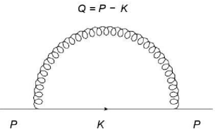
Figure 1: One-loop quark self energy in hot and magnetized medium

The quark propagator in presence of background magnetic field following the Schwinger formalism can be written in terms of Laguerre polynomial ($L_{l}(2\alpha)$) [72]

$$iS(K)=\sum_{l=0}^{\infty}\frac{-id_{l}(\alpha)D+d^{\prime}_{l}(\alpha)\bar{D}}{k_{L}^{2}+2l|q_{f}B|}+\frac{i\gamma.k_{\perp}}{k_{\perp}^{2}},$$ (10)

where $q_{f}$ is the absolute charge of $f$th flavor, $l$ = 0, 1, 2, $\dots$ are the Landau levels, $||$ and $\perp$ are the parallel and perpendicular components of momentum respectively with respect to direction of magnetic field, $\alpha=k_{\perp}^{2}/|q_{f}B|$, $k_{L}^{2}=m_{f0}^{2}-k_{||}^{2}$ and $d_{l}(\alpha),d^{\prime}_{l}(\alpha),D,\bar{D}$ are given as [73],

$$d_{l}(\alpha)=(-1)^{l}e^{-\alpha}C_{l}(2\alpha),$$

$$d^{\prime}_{l}(\alpha)=\frac{\partial d_{l}}{\partial\alpha},$$

$$D=(m_{f0}+\gamma.k_{||})+\gamma.k_{\perp}\left(\frac{m_{f0}^{2}-k_{||}^{2}}{k_{\perp}^{2}}\right),$$

$$\bar{D}=\gamma_{1}\gamma_{2}\left(m_{f0}+\gamma.k_{||}\right),$$ (11)

with $C_{l}(2\alpha)=L_{l}(2\alpha)-L_{l-1}(2\alpha)$. In weak field limit, the quark propagator can be reorganized in power series of magnetic field $\left({\bf{q_{f}B}}\right)$ as,

$$iS(K)=\frac{i\left(\not{K}+m_{f0}\right)}{K^{2}-m_{f0}^{2}}-\frac{\gamma_{1}\gamma_{2}\left(\gamma.K_{||}+m_{f0}\right)}{\left(K^{2}-m_{f0}^{2}\right)^{2}}(q_{f}B),$$ (12)

where first term in Eq.(12) is the free fermion propagator and second term is the $\mathcal{O}(q_{f}B)$ correction to it. Neglecting the current quark mass under the limit $\left(m_{f0}^{2}<q_{f}B<T^{2}\right)$ in the numerator and using the following metric tensor in Eq.(12),

$$g^{\mu\nu}= g^{\mu\nu}_{||}+g^{\mu\nu}_{\bot};$$

$$g^{\mu\nu}_{\parallel}=\text{diag}(1,0,0,-1); \quad g^{\mu\nu}_{\bot}=\text{diag}(0,-1,-1,0);$$

$$p^{\mu}=p^{\mu}_{\parallel}+p^{\mu}_{\bot}; \quad p^{\mu}_{\parallel}=(p^{0},0,0,p^{3});$$

$$p^{\mu}_{\bot}=(0,p^{1},p^{2},0); \quad\not{p}=\gamma^{\mu}p_{\mu}=\not{p}_{\parallel}+\not{p}_{\bot};$$

$$\not{p}_{\parallel}=\gamma^{0}p_{0}-\gamma^{3}p^{3}; \quad\not{p}_{\bot}=\gamma^{1}p^{1}+\gamma^{2}p^{2},$$ (13)

with

$$i\gamma_{1}\gamma_{2}\not{K}_{||}=-\gamma_{5}[(K.b)\not{u}-(K.u)\not{b}],$$ (14)

we obtain the quark propagator in presence of magnetic field at finite temperature as

$$iS(K)=\frac{i\not{K}}{K^{2}-m_{f0}^{2}}-\frac{i\gamma_{5}[(K.b)\not{u}-(K.u)\not{b}]}{(K^{2}-m_{f0}^{2})^{2}}\big{(}q_{f}B\big{)},$$ (15)

where $u^{\mu}=(1,0,0,0)$ denotes local rest frame of the heat bath. Introduction of a particular frame of reference breaks the Lorentz symmetry of the system. Similarly, $b^{\mu}=(0,0,0,1)$ denotes the preferred direction of magnetic field in our system which then breaks the rotational symmetry of the system. Using the quark propagator (15), the one-loop quark self energy upto $\mathcal{O}(q_{f}B)$ in hot and weakly magnetized medium can be written as

$$\Sigma(P)=g^{2}C_{F}T\sum_{n}\int\frac{d^{3}k}{(2\pi)^{3}}\gamma_{\mu}\Bigg{(}\frac{\not{K}}{(K^{2}-m_{f0}^{2})}- \frac{\gamma_{5}[(K.b)\not{u}-(K.u)\not{b}]}{(K^{2}-m_{f0}^{2})^{2}}(q_{f}B)\Bigg{)}\times$$

$$\gamma^{\mu}\frac{1}{(P-K)^{2}},$$ (16)

where $T$ is the temperature of the system and $g^{2}=4\pi\alpha_{s}(\Lambda^{2},|eB|)$. First term is the thermal medium contribution ($\Sigma_{0}$) whereas second one is with magnetic field correction term ($\Sigma_{1}$).

The general covariant structure of quark self energy at finite temperature and magnetic field can be written as [66]

$$\Sigma(P)=-\mathcal{A}\not{P}-\mathcal{B}\not{u}-\mathcal{C}\gamma_{5}\not{u}-\mathcal{D}\gamma_{5}\not{b},$$ (17)

where $\mathcal{A},\mathcal{B},\mathcal{C},\mathcal{D}$ are the structure functions. Using Eq.(II) and (17), the general form of these structure functions are obtained as

$$\mathcal{A}\left(p_{0},p_{\perp},p_{z}\right)=\frac{1}{4}\frac{\text{Tr}(\Sigma(P)\not{P})-(P.u)\text{Tr}(\Sigma(P)\not{u})}{(P.u)^{2}-P^{2}},$$ (18)

$$\mathcal{B}\left(p_{0},p_{\perp},p_{z}\right)=\frac{1}{4}\frac{\left(-P.u\right)\text{Tr}(\Sigma(P)\not{P})+P^{2}\text{Tr}(\Sigma(P)\not{u})}{(P.u)^{2}-P^{2}},$$ (19)

$$\mathcal{C}\left(p_{0},p_{\perp},p_{z}\right)=-\frac{1}{4}\text{Tr}(\gamma_{5}\Sigma(P)\not{u}),$$ (20)

$$\mathcal{D}\left(p_{0},p_{\perp},p_{z}\right)=\frac{1}{4}\text{Tr}(\gamma_{5}\Sigma(P)\not{b}).$$ (21)

These structure functions are found to depend upon various Lorentz scalars defined by

$$p^{0}\equiv P^{\mu}u_{\mu}=\omega,$$ (22)

$$p^{3}\equiv P^{\mu}b_{\mu}=-p_{z},$$ (23)

$$p_{\bot}\equiv\big{[}(P^{\mu}u_{\mu})^{2}-(P^{\mu}b_{\mu})^{2}-(P^{\mu}P_{\mu})^{2}\big{]}^{1/2},$$ (24)

where $\omega,p_{\bot},p_{z}$ are termed as Lorentz invariant energy, transverse momentum and longitudinal momentum respectively. The detailed calculation of all these structure functions is shown in Appendix A and results are quoted here,

$$\mathcal{A}(p_{0},|{\bf{p}}|)=\frac{m_{th}^{2}}{|{\bf{p}}|^{2}}Q_{1}\Bigg{(}\frac{p_{0}}{|{\bf{p}}|}\Bigg{)},$$ (25)

$$\mathcal{B}(p_{0},|{\bf{p}}|)=-\frac{m_{th}^{2}}{|{\bf{p}}|}\Bigg{[}\frac{p_{0}}{|{\bf{p}}|}Q_{1}\Big{(}\frac{p_{0}}{|{\bf{p}}|}\Big{)}-Q_{0}\Bigg{(}\frac{p_{0}}{|{\bf{p}}|}\Bigg{)}\Bigg{]},$$ (26)

$$\mathcal{C}(p_{0},|{\bf{p}}|)=-4g^{2}C_{F}M^{2}\frac{p_{z}}{|{\bf{p}}|^{2}}Q_{1}\Bigg{(}\frac{p_{0}}{|{\bf{p}}|}\Bigg{)},$$ (27)

$$\mathcal{D}(p_{0},|{\bf{p}}|)=-4g^{2}C_{F}M^{2}\frac{1}{|{\bf{p}}|}Q_{0}\Bigg{(}\frac{p_{0}}{|{\bf{p}}|}\Bigg{)},$$ (28)

where $Q_{0}$ and $Q_{1}$ are Legendre functions of first and second kind respectively read as

$$Q_{0}(x)=\frac{1}{2}\ln\left(\frac{x+1}{x-1}\right),$$ (29)

$$Q_{1}(x)=\frac{x}{2}\ln\left(\frac{x+1}{x-1}\right)-1=xQ_{0}(x)-1,$$ (30)

with magnetic mass obtained as [74]

$$M^{2}(T,\mu,m_{f0},q_{f}B)=\frac{|q_{f}B|}{16\pi^{2}}\left(\frac{\pi T}{2m_{f0}}-\text{ln}2+\frac{7\mu^{2}\zeta(3)}{8\pi^{2}T^{2}}\right).$$ (31)

where $\zeta$ is the Riemann zeta function. The general covariant structure of quark self energy Eq.(17) can be recast in terms of left handed ($P_{L}=(\mathbb{I}-\gamma_{5})/2$) and right handed ($P_{R}=(\mathbb{I}+\gamma_{5})/2$) chiral projection operators as

$$\Sigma(P)=-P_{R}\not{A^{\prime}}P_{L}-P_{L}\not{B^{\prime}}P_{R},$$ (32)

with $\not{A^{\prime}}$ and $\not{B^{\prime}}$ defined as

$$\not{A^{\prime}}=\mathcal{A}\not{P}+(\mathcal{B}+\mathcal{C})\not{u}+\mathcal{D}\not{b},$$ (33)

$$\not{B^{\prime}}=\mathcal{A}\not{P}+(\mathcal{B}-\mathcal{C})\not{u}-\mathcal{D}\not{b}.$$ (34)

Using Eq.(II) and (32), inverse fermion propagator can be written as

$$S^{*-1}(P)=\not{P}+P_{R}\left[\mathcal{A}\not{P}+\left(\mathcal{B}+\mathcal{C}\right)\not{u}+\mathcal{D}\not{b}\right]P_{L}+P_{L}\left[\mathcal{A}\not{P}+\left(\mathcal{B}-\mathcal{C}\right)\not{u}-\mathcal{D}\not{b}\right]P_{R},$$ (35)

and using $P_{L,R}\gamma^{\mu}=\gamma^{\mu}P_{R,L}$ and $P_{L}\not{P}P_{L}=P_{R}\not{P}P_{R}=P_{L}P_{R}\not{P}=0$, we obtain

$$S^{*-1}(P)=P_{R}\not{L}P_{L}+P_{L}\not{R}P_{R},$$ (36)

where $\not{L}$ and $\not{R}$ are

$$\not{L}=(1+\mathcal{A})\not{P}+(\mathcal{B}+\mathcal{C})\not{u}+\mathcal{D}\not{b},$$ (37)

$$\not{R}=(1+\mathcal{A})\not{P}+(\mathcal{B}-\mathcal{C})\not{u}-\mathcal{D}\not{b}.$$ (38)

Thus, we get the effective quark propagator as

$$S^{*}(P)=\frac{1}{2}\left[P_{L}\frac{\not{L}}{L^{2}/2}P_{R}+P_{R}\frac{\not{R}}{R^{2}/2}P_{L}\right],$$ (39)

where

$$L^{2}=(1+\mathcal{A})^{2}P^{2}+2(1+\mathcal{A})(\mathcal{B}+\mathcal{C})p_{0}-2\mathcal{D}(1+\mathcal{A})p_{z}+(\mathcal{B}+\mathcal{C})^{2}-\mathcal{D}^{2},$$ (40)

$$R^{2}=(1+\mathcal{A})^{2}P^{2}+2(1+\mathcal{A})(\mathcal{B}-\mathcal{C})p_{0}+2\mathcal{D}(1+\mathcal{A})p_{z}+(\mathcal{B}-\mathcal{C})^{2}-\mathcal{D}^{2}.$$ (41)

Next, we take the static limit ($p_{0}=0,|{\bf{p}}|\rightarrow 0$) of $L^{2}/2$ and $R^{2}/2$, after expanding the Legendre functions involved in structure functions in power series of $\frac{|\bf{p}|}{p_{0}}$. Considering upto $\mathcal{O}(g^{2})$, we obtain

$$\frac{L^{2}}{2}\arrowvert_{p_{0}=0,{|\bf{p}|}\rightarrow 0}=m_{th}^{2}+4g^{2}C_{F}M^{2},$$ (42)

$$\frac{R^{2}}{2}|_{p_{0}=0,{|\bf{p}|}\rightarrow 0}=m_{th}^{2}-4g^{2}C_{F}M^{2}.$$ (43)

The degenerate left- and right- handed modes get separated out in presence of weak magnetic field and hence the thermal mass (squared) at finite chemical potential in presence of weak magnetic field obtained as

$$m_{L}^{2}=m_{th}^{2}+4g^{2}C_{F}M^{2},$$ (44)

$$m_{R}^{2}=m_{th}^{2}-4g^{2}C_{F}M^{2},$$ (45)

which is opposite to the case of strong magnetic field where left- and right-handed chiral modes have the same mass [62]. The quasiparticle mass obtained above consists of pure thermal and magnetic contributions. The thermal mass is independent of chiral modes whereas magnetic contribution depends on the chiral modes. The dispersion relation for both chiral modes of quarks at low and high momentum limit in lowest Landau level is given by [66]

$$\omega_{L/R}(p_{z})=m_{L/R}+\frac{p_{z}}{3};\qquad(p_{z}<<m_{L/R})$$ (46)

$$\omega_{L/R}(p_{z})=|p_{z}|+\frac{m_{L/R}^{2}}{p_{z}};\qquad(p_{z}>>m_{L/R}).$$ (47)

The form of dispersion relations in both low and high momentum limits even in the presence of magnetic field is similar to that in the absence of magnetic field and the masses in both the limits are of the same order. However, the quasiparticle mass used in our computation is obtained from the static limit of the pole of the full quark propagator (up to one-loop quark self energy), which is independent of low momentum and high momentum limits. Now, we will evaluate the charge and thermal transport coefficients in the presence of weak magnetic field at finite chemical potential for left- and right-handed modes separately as the system will not be in both modes simultaneously.

III CHARGE TRANSPORT COEFFICIENTS

Boltzmann transport equation governs the evolution of phase space density $f(x,p)$ associated with the partons in our system. The QGP is a relativistic plasma, since $T>>$ any mass scale in the system. This validates the use of the relativistic Boltzmann transport equation (RBTE) to carry out our investigation. The RBTE for relativistic particle with charge $q$ in presence of external electromagnetic field can be written as [75]

$$p^{\mu}\partial_{\mu}f(x,p)+qF^{\mu\nu}p_{\nu}\frac{\partial f(x,p)}{\partial p^{\mu}}=C[f],$$ (48)

where, $f$ is the distribution function deviated slightly from equilibrium distribution function ($f_{0}$) with $f=f_{0}+\delta f$ ($\delta f<<f_{0}$). $F^{\mu\nu}$ is the anti-symmetric electromagnetic field tensor, $C[f]$ is the collision integral that describes the rate of change of distribution function by virtue of collisions. The general form of collision integral consists of absorption and emission terms in phase space volume element. This leads to nonlinear integro-differential equation which is very complicated to solve. Hence, we simplify the equation using relaxation-time approximation (RTA). Under relaxation time approximation, the external perturbation takes the system slightly away from equilibrium from which it relaxes towards the equilibrium exponentially with time scale $\tau$. Collision integral under RTA takes the form as

$$C[f]\simeq-\frac{p^{\mu}u_{\mu}}{\tau}(f-f_{0})\equiv-\frac{p^{\mu}u_{\mu}}{\tau}\delta f,$$ (49)

where $u_{\mu}$ is the fluid 4-velocity, $\tau$ is the thermal averaged relaxation time. The Eq.(48) in 3-notation can be written as

$$\frac{\partial f}{\partial t}+{\bf{v}}.\frac{\partial f}{\partial\bf{r}}+{q(\bf{E+v\times B})}.\frac{\partial f}{\partial\bf{p}}=-\frac{1}{\tau}(f-f_{0}).$$ (50)

We consider the spatially uniform $\frac{\partial f}{\partial{\bf{r}}}\approx 0$ and static medium $\frac{\partial f}{\partial t}=0$ such that there are no space-time gradient. Then Eq.(50) simplifies to

$$q({\bf{E+v\times B}}).\frac{\partial f}{\partial{\bf{p}}}=-\frac{1}{\tau}(f-f_{0}).$$ (51)

For the sake of simplicity of calculation, we choose the transverse electric and magnetic field as ${\bf{E}}=E\hat{x}$ and ${\bf{B}}=B\hat{z}$. This yields:

$$f-qB\tau\Big{(}v_{x}\frac{\partial f}{\partial p_{y}}-v_{y}\frac{\partial f}{\partial p_{x}}\Big{)}=f_{0}-qE\tau\frac{\partial f_{0}}{\partial p_{x}}.$$ (52)

In order to solve Eq.(52), we take the following ansatz of distribution function $f(p)$ as [76]

$$f(p)=f_{0}-\tau q{\bf{E}}.\frac{\partial f_{0}}{\partial{\bf{p}}}-{\bm{\xi}}.\frac{\partial f_{0}}{\partial{\bf{p}}},$$ (53)

and $f_{0}$ is given by,

$$f_{0}({\bf{p}})=\frac{1}{e^{(\sqrt{{\bf{p^{2}}}+m^{2}}-\mu)/T}+1},$$ (54)

which is space and time independent solution to the Boltzmann equation and $f_{0}$ satisfies,

$$\frac{\partial f_{0}}{\partial\bf{p}}={\bf{v}}\frac{\partial f_{0}}{\partial\varepsilon},\quad\frac{\partial f_{0}}{\partial\varepsilon}=-\beta f_{0}(1-f_{0}),$$ (55)

where $\varepsilon=\sqrt{{\bf{p^{2}}}+m^{2}}$ is the single particle energy. Using the ansatz Eq.(53) in Eq.(52), we get

$$\left(f_{0}-\tau q{\bf{E}}.\frac{\partial f_{0}}{\partial{\bf{p}}}-\bm{\xi}.\frac{\partial f_{0}}{\partial\bf{p}}\right)-qB\tau\left(v_{x}\frac{\partial}{\partial p_{y}}-v_{y}\frac{\partial}{\partial p_{x}}\right) \left(f_{0}-\tau q{\bf{E}}.\frac{\partial f_{0}}{\partial{\bf{p}}}-\bm{\xi}.\frac{\partial f_{0}}{\partial\bf{p}}\right)$$

$$=f_{0}-qE\tau\frac{\partial f_{0}}{\partial p_{x}}.$$ (56)

The first term in the parenthesis in left hand side of Eq.(III) can be rewritten as,

$$\left(f_{0}-\tau q{\bf{E}}.\frac{\partial f_{0}}{\partial{\bf{p}}}-\bm{\xi}.\frac{\partial f_{0}}{\partial\bf{p}}\right)=f_{0}+\beta\tau qEv_{x}f_{0}+(\bm{\xi}.{\bf{v}})\beta f_{0}.$$ (57)

Neglecting the $f_{0}^{2}$ terms at high temperature and using the following second order partial derivatives,

$$\frac{\partial^{2}f_{0}}{\partial p_{y}p_{x}}=\frac{\beta p_{x}p_{y}f_{0}}{\varepsilon^{2}}\left(\beta+\frac{1}{\varepsilon}\right),$$ (58)

$$\frac{\partial^{2}f_{0}}{\partial p_{y}p_{z}}=\frac{\beta p_{y}p_{z}f_{0}}{\varepsilon^{2}}\left(\beta+\frac{1}{\varepsilon}\right),$$ (59)

$$\frac{\partial^{2}f_{0}}{\partial p_{y}^{2}}=-\beta\left[\frac{f_{0}}{\varepsilon}-\frac{f_{0}p_{y}^{2}}{\varepsilon^{2}}\left(\beta+\frac{1}{\epsilon}\right)\right],$$ (60)

the second term in left hand side of Eq.(III) get reduced to

$$qB\tau\left(v_{x}\frac{\partial}{\partial p_{y}}-v_{y}\frac{\partial}{\partial p_{x}}\right)\left(f_{0}-\tau q{\bf{E}}.\frac{\partial f_{0}}{\partial{\bf{p}}}-\bm{\xi}.\frac{\partial f_{0}}{\partial\bf{p}}\right)=qB\tau\beta\left(\frac{\xi_{y}v_{x}}{\varepsilon}-\frac{\xi_{x}v_{y}}{\varepsilon}-\frac{v_{y}\tau qE}{\varepsilon}\right)f_{0}.$$ (61)

Combining the Eq.(57) and (61), Eq.(III) obtained as

$$\frac{\tau qBqEv_{y}}{\varepsilon}-\frac{qB}{\varepsilon}(v_{x}\xi_{y}-v_{y}\xi_{x})+\frac{1}{\tau}\Big{(}\xi_{x}\frac{p_{x}}{\varepsilon}+\xi_{y}\frac{p_{y}}{\varepsilon}+\xi_{z}\frac{p_{z}}{\varepsilon}\Big{)}=0.$$ (62)

The above equation should be satisfied for any value of velocity therefore, comparing the coefficients of $v_{x},v_{y}$ and $v_{z}$ of Eq.(62), we get

$$\xi_{z}=0,$$ (63)

$$\omega_{c}\tau qE+\omega_{c}\xi_{x}+\frac{\xi_{y}}{\tau}=0,$$ (64)

$$\frac{\xi_{x}}{\tau}-\omega_{c}\xi_{y}=0,$$ (65)

where $\omega_{c}=\frac{qB}{\varepsilon}$ is termed as cyclotron frequency. Solving for $\xi_{x}$ and $\xi_{y}$, we have

$$\xi_{x}=\frac{-\omega_{c}^{2}\tau^{3}qE}{(\omega_{c}^{2}\tau^{2}+1)};\quad\xi_{y}=\frac{-\omega_{c}\tau^{2}qE}{(\omega_{c}^{2}\tau^{2}+1)}.$$ (66)

Using Eq.(80) in Eq.(53), the distribution function $f(p)$ for quarks simplifies to

$$f(p)=f_{0}-\frac{qEv_{x}\tau}{(1+\omega_{c}^{2}\tau^{2})}\left(\frac{\partial f_{0}}{\partial\varepsilon}\right)+\frac{qEv_{y}\omega_{c}\tau^{2}}{(1+\omega_{c}^{2}\tau^{2})}\left(\frac{\partial f_{0}}{\partial\varepsilon}\right),$$ (67)

and for anti-quarks ($f\rightarrow\bar{f},q\rightarrow-q,\omega_{c}\rightarrow-\omega_{c}$),

$$\bar{f}(p)=\bar{f_{0}}+\frac{qEv_{x}\tau}{(1+\omega_{c}^{2}\tau^{2})}\left(\frac{\partial\bar{f_{0}}}{\partial\varepsilon}\right)+\frac{qEv_{y}\omega_{c}\tau^{2}}{(1+\omega_{c}^{2}\tau^{2})}\left(\frac{\partial\bar{f_{0}}}{\partial\varepsilon}\right).$$ (68)

The induced current in the system as a result of external electromagnetic fields can be written as

$$j^{i}=\sigma_{\text{Ohmic}}\delta^{ij}E_{j}+\sigma_{\text{Hall}}\epsilon^{ij}E_{j},$$ (69)

where $\sigma_{\text{Ohmic}}$ and $\sigma_{\text{Hall}}$ are Ohmic and Hall conductivities respectively, $\epsilon_{ij}$ is the $2\times 2$ antisymmetric unity tensor, with $\epsilon_{12}=-\epsilon_{21}=1$. It is clear from the above equation that $\sigma_{{\text{Ohmic}}}$ describes the longitudinal response (current along the direction of electric field) and $\sigma_{{\text{Hall}}}$ describes the transverse response (current transverse to the electric field). Further, the induced current can be written in terms of deviation $\delta f$ ($\delta\bar{f}$) from $f_{0}$ ($\bar{f_{0}}$) as

$${\bf{j}}=g_{f}\int\frac{d^{3}{p}}{(2\pi)^{3}}{\bf{v}}\left(q\delta f(p)+\bar{q}\delta\bar{f}(p)\right),$$ (70)

where $\bar{q}$ is the charge of antiparticle and $g_{f}=3\times 2$ is the color and spin degeneracy factor of fermions. Using Eq.(69) and (70), the Ohmic and Hall conductivity for a system of multiple charge species can be written as

$$\sigma_{{\text{Ohmic}}}=\frac{1}{6\pi^{2}T}\sum_{f}g_{f}q^{2}_{f}\tau_{f}\int dp\frac{p^{4}}{\varepsilon_{f}^{2}}\frac{1}{(1+\omega_{c}^{2}\tau_{f}^{2})}[f^{0}_{f}(1-f^{0}_{f})+\bar{f^{0}_{f}}(1-\bar{f^{0}_{f}})],$$ (71)

$$\sigma_{{\text{Hall}}}=\frac{1}{6\pi^{2}T}\sum_{f}g_{f}q^{2}_{f}\tau_{f}^{2}\int dp\frac{p^{4}}{\varepsilon_{f}^{2}}\frac{\omega_{c}}{(1+\omega_{c}^{2}\tau_{f}^{2})}[f^{0}_{f}(1-f^{0}_{f})-\bar{f^{0}_{f}}(1-\bar{f^{0}_{f}})],$$ (72)

where $f$ stands for flavor and here we have used $f=$ up ($u$), down ($d$). The relaxation time for quarks (antiquarks) used above for calculation of conductivities is given by [77], where massless $u$- and $d$-quarks were considered with $\mu<<T$,

$$\tau_{q(\bar{q})}=\frac{1}{5.1T\alpha_{s}^{2}\log(\frac{1}{\alpha_{s}})(1+0.12(2N_{f}+1))}.$$

It was argued in [78] that finite parton mass has little effect on scattering cross-section and hence on relaxation time. This leads to qualitatively same result for massless and massive partons. The current light quark ($m_{u,d}$) masses are chosen to be $0.1$ times the strange quark mass ($m_{s0}$) which is in compliant with chiral perturbation theory [79, 80]. The parameters were adjusted to get the best fitted lattice data with $m_{s0}=80$MeV [81]. The Ohmic and Hall conductivity obtained above is defined by current which appears due to the effect of an electric and magnetic field when there is no temperature gradient or we can say isothermal Ohmic and Hall conductivity. As discussed in quasiparticle model, we will incorporate the quasiparticle mass which were obtained to be different for left- and right-handed chiral modes. $u(\bar{u})$ and $d(\bar{d})$ quarks are spin-$\frac{1}{2}$ particles and they can assume right-handedness or left-handedness depending on their up or down spin with respect to their direction of motion. We have taken into account the both modes for up and down quarks and computed the conductivities for L- and R-mode separately. In case of baryonic symmetry i.e. at zero quark chemical potential, the distribution function for quarks and anti-quarks become equal and hence Hall conductivity vanishes.

IV HEAT TRANSPORT COEFFICIENTS

In nonrelativistic case, the heat equation is obtained by the validity of the first and second laws of thermodynamics, where the flow of heat is proportional to the temperature gradient and the proportionality factor is called the thermal conductivity. We are intended to study the thermal conductivity in the system of partons. The heat flow 4-vector which is defined to be difference between energy diffusion and enthalpy diffusion is given as [82],

$$Q_{\mu}=\Delta_{\mu\alpha}T^{\alpha\beta}u_{\beta}-h\Delta_{\mu\alpha}N^{\alpha},$$ (73)

where $\Delta_{\mu\alpha}=g_{\mu\alpha}-u_{\mu}u_{\alpha}$ is the projection operator. $N^{\alpha}$ is characterized as first moment of distribution function which corresponds to the particle four-flow vector as

$$N^{\alpha}=\sum_{f}g_{f}\int\frac{d^{3}p}{(2\pi)^{3}}\frac{p^{\alpha}}{\varepsilon_{f}}\left[f_{f}-\bar{f}_{f}\right],$$ (74)

whereas, $T^{\alpha\beta}$ is characterized as second moment of distribution function which corresponds to energy-momentum tensor as

$$T^{\alpha\beta}=\sum_{f}g_{f}\int\frac{d^{3}p}{(2\pi)^{3}}\frac{p^{\alpha}p^{\beta}}{\varepsilon_{f}}\left(f_{f}+\bar{f}_{f}\right)+g_{g}\int\frac{d^{3}p}{(2\pi)^{3}}\frac{p^{\alpha}p^{\beta}}{\varepsilon_{g}}f_{g},$$ (75)

where, $f_{f},\bar{f}_{f}$ and $f_{g}$ are quark, antiquark and gluon distribution function, $\varepsilon_{g}$ is the single particle energy for gluons and $g_{g}=8\times 2$ is the degeneracy factor of the gluons. We can obtain the particle number density, energy density and pressure from the above equation as $n=N^{\alpha}u_{\alpha}$, $e=u_{\alpha}T^{\alpha\beta}u_{\beta}$ and $P=-\Delta_{\alpha\beta}T^{\alpha\beta}/3$ respectively. Therefore, enthalpy per particle can be obtained as, $h=(e+P)/n$. The heat flow 4-vector in rest frame of heat bath is orthogonal to fluid 4-velocity, i.e. $Q_{\mu}u^{\mu}=0$. Thus, heat flow is spatial which can be written in terms of infinitesimal changes in the distribution function as

$${\bf{Q}}=\sum_{f}g_{f}\int\frac{d^{3}p}{(2\pi)^{3}}\frac{{\bf{p}}}{\varepsilon_{f}}\left[\left(\varepsilon_{f}-h_{f}\right)\delta f_{f}+\left(\varepsilon_{f}+\bar{h}_{f}\right)\delta\bar{f}_{f}\right]+g_{g}\int\frac{d^{3}p}{(2\pi)^{3}}{\bf{p}}\delta f_{g}.$$ (76)

The particle four-flow and energy-momentum tensor can be decomposed with respect to an arbitrary normalized time-like four vector, $u^{\mu}=\gamma(1,\vec{v})$, where $u^{\mu}u_{\mu}=1$. The most general decomposition is given as [83, 84]

$$N^{\mu}=nu^{\mu}+v^{\mu},$$ (77)

$$T^{\mu\nu}=-Pg^{\mu\nu}+wu^{\mu}u^{\nu}+\pi^{\mu\nu},$$ (78)

where, $v^{\mu}$ is the particle diffusion current, $w=e+P$ is the heat function per unit volume, $\pi^{\mu\nu}$ is the shear-stress tensor. Using the continuity equation and law of increase of entropy, the required form of symmetrical 4-tensor $\pi^{\mu\nu}$ and 4-vector $v^{\mu}$ obtained to be as [83],

$$\pi^{\mu\nu}=-c\eta\left(\frac{\partial u^{\mu}}{\partial x_{\nu}}+\frac{\partial u^{\nu}}{\partial x_{\mu}}-u^{\mu}u_{\alpha}\frac{\partial u^{\nu}}{\partial x_{\alpha}}-u^{\mu}u^{\alpha}\frac{\partial u^{\mu}}{\partial x^{\alpha}}\right)-\left(\zeta-\frac{2}{3}\eta\right)\frac{\partial u^{\alpha}}{\partial x^{\alpha}}\left(g^{\mu\nu}-u^{\mu}u^{\nu}\right),$$ (79)

$$v^{\mu}=\frac{\kappa}{c}\left(\frac{nT}{w}\right)^{2}\left[\frac{\partial}{\partial x_{\mu}}\left(\frac{\mu}{T}\right)-u^{\mu}u^{\alpha}\frac{\partial}{\partial x^{\alpha}}\left(\frac{\mu}{T}\right)\right].$$ (80)

Here, $\eta$ and $\zeta$ are shear and bulk viscosity coefficients and $\kappa$ is the thermal conductivity, taken in accordance with their non-relativistic definitions. The zero particle flux ($nu^{i}+v^{i}=0$) corresponds to the pure thermal conduction. The spatial components $u^{i}=-v^{i}/n$ of the 4-velocity are of the first order in the gradients; since $\pi^{\mu\nu},v^{\mu}$ are written only as far as this order, the 4-velocity component $u^{0}$ must be taken as unity. To the same accuracy, omitting the second term in the square bracket of Eq.(80), the energy flux density from $T^{\mu\nu}$ is given as,

$$cT^{0i}=cwu^{0}u^{i}=-cwv^{i}/n$$ (81)

$$=-\kappa\frac{nT^{2}}{e+P}\left[\frac{\partial}{\partial x_{i}}\left(\frac{\mu}{T}\right)\right],$$

which relates the energy flux density/heat flow with the gradient of thermodynamical potential ($U=\mu/T$) as in Navier-Stokes theory. In terms of 4-gradient, the above equation can be written as

$$Q_{\mu}= -\kappa\frac{nT^{2}}{e+P}\nabla_{\mu}U,$$ (82)

where $\kappa$ is the thermal conductivity and $\nabla_{\mu}$ is the 4-gradient, $\nabla_{\mu}=\partial_{\mu}-u_{\mu}u_{\nu}\partial^{\nu}$. The entropy density ($s=s(e,n)$) in equilibrium state in terms of energy density, pressure and chemical potential can be written as [85],

$$s=\left(\frac{e+P}{T}\right)-\left(\frac{\mu}{T}\right)n.$$ (83)

Further, the inverse of temperature ($T^{-1}$) and thermodynamic potential ($U$) can be defined as partial derivative of $s(e,n)$

$$\text{d}s=\frac{1}{T}\text{d}e-U\text{d}n.$$ (84)

Using Eq.(83) and (84), we obtain

$$\text{d}\left(\frac{P}{T}\right)=-e\text{d}\left(\frac{1}{T}\right)+n\text{d}U,$$

$$\frac{\text{d}P}{nT}=\text{d}U+\frac{1}{T^{2}}\left(\frac{P+e}{n}\right)\text{d}T.$$ (85)

Generalizing it to the 4-gradient, the heat flow can be rewritten as

$$Q_{\mu}=\kappa\left[\nabla_{\mu}T-\frac{T}{e+P}\nabla_{\mu}P\right],$$ (86)

and in local rest frame, the spatial component of heat flow can be written as

$${\bf{Q}}=-\kappa\left[\frac{\partial T}{\partial{\bf{x}}}-\frac{T}{nh}\frac{\partial P}{\partial{\bf{x}}}\right].$$ (87)

One can thus obtain the thermal conductivity ($\kappa$) by comparing Eq.(76) and Eq.(87). We will firstly calculate the contribution of quarks and anti-quarks to the thermal conductivity. So now, expressing the relativistic Boltzmann transport equation in terms of gradients of flow velocity and temperature in relaxation time approximation as

$$p^{\mu}\partial_{\mu}T\left(\frac{\partial f}{\partial T}\right)+ p^{\mu}\partial_{\mu}(p^{\nu}u_{\nu})\left(\frac{\partial f}{\partial p^{0}}\right)+q\Bigg{(}F^{0j}p_{j}\frac{\partial f}{\partial p^{0}}+F^{j0}p_{0}\frac{\partial f}{\partial p^{j}}+$$

$$F^{ij}p_{j}\frac{\partial f}{\partial p^{i}}+F^{ji}p_{i}\frac{\partial f}{\partial p^{j}}\Bigg{)}=-\frac{p^{\mu}u_{\mu}}{\tau}\delta f,$$ (88)

where $p_{0}=\varepsilon-\mu$ and for very small $\mu$, it can be approximated as $p_{0}\approx\varepsilon$. Using the following partial derivatives

$$\frac{\partial f_{0}}{\partial T}=\frac{\varepsilon}{T^{2}}f_{0}(1-f_{0}),$$ (89)

$$\frac{\partial f_{0}}{\partial p^{0}}=-\frac{1}{T}f_{0}(1-f_{0}),$$ (90)

$$\frac{\partial f_{0}}{\partial p_{j}}=-\frac{p_{j}}{Tp_{0}}f_{0}(1-f_{0}),$$ (91)

the Eq.(IV) is given as

$$-\frac{\delta f}{\tau}= \frac{f_{0}(1-f_{0})}{p^{0}}\left[p^{\mu}\partial_{\mu}T\left(\frac{p^{0}}{T^{2}}\right)-\frac{p^{\mu}\partial_{\mu}(p^{\nu}u_{\nu})}{T}-\frac{q}{T}\left(F^{0j}p_{j}+F^{j0}p_{j}\right)\right]+\frac{q}{p^{0}}\left(F^{ij}p_{j}\frac{\partial f}{\partial p^{i}}+F^{ji}p_{i}\frac{\partial f}{\partial p^{j}}\right)$$

$$=\frac{1}{T}f_{0}(1-f_{0})\Bigg{[}\frac{1}{T}\left(p^{0}\partial_{0}T+p^{j}\partial_{j}T\right)+T\partial_{0}\left(\frac{\mu}{T}\right)+\frac{p^{j}T}{p^{0}}\partial_{j}\left(\frac{\mu}{T}\right)-\frac{1}{p^{0}}\left(p^{0}p^{\nu}\partial_{0}u_{\nu}+p^{j}p^{\nu}\partial_{j}u_{\nu}\right)-$$

$$2q\frac{\textbf{E.p}}{p^{0}}\Bigg{]}+q\left(\textbf{v}\mathbb{\times}\textbf{B}\right).\frac{\partial f}{\partial\textbf{p}},$$ (92)

where $2F_{ij}=\epsilon_{ijk}B^{k}$. Now, exerting the energy-momentum conservation $\left(\partial_{0}u_{\mu}=\frac{\nabla_{\mu}P}{nh}\right)$ along with relativistic Gibbs-Duhem relation,

$$\partial_{j}\left(\frac{\mu}{T}\right)=\frac{-h}{T^{2}}\left(\partial_{j}T-\frac{T}{nh}\partial_{j}P\right),$$

we obtain Eq.(IV) as

$$-\frac{\delta f}{\tau}=\frac{1}{T}f_{0}(1-f_{0})\Bigg{[}\frac{1}{T} \left(p^{0}\partial_{0}T\right)+\left(\frac{p^{0}-h}{p^{0}}\right)\frac{p^{j}}{T}\left(\partial_{j}T-\frac{T}{nh}\partial_{j}P\right)+T\partial_{0}\left(\frac{\mu}{T}\right)-p^{j}p^{\nu}\left(\partial_{j}u_{\nu}\right)-2q\frac{\textbf{E.p}}{p^{0}}\Bigg{]}$$

$$+q\left(\textbf{v}\mathbb{\times}\textbf{B}\right).\frac{\partial f}{\partial\textbf{p}},$$ (93)

where $\frac{\partial f}{\partial\textbf{p}}=\frac{\partial}{\partial\textbf{p}}\left(f_{0}+\delta f\right)$ and $\frac{\partial f_{0}}{\partial p^{j}}\propto v^{j}$, therefore the Lorentz term vanishes for the equilibrium distribution function and we get,

$$-\frac{\delta f}{\tau}= \frac{1}{T}f_{0}(1-f_{0})\Bigg{[}\frac{p_{0}}{T}\partial_{0}T+\left(\frac{p^{0}-h}{p^{0}}\right)\frac{p^{j}}{T}\left(\partial_{j}T-\frac{T}{nh}\partial_{j}P\right)+T\partial_{0}\Big{(}\frac{\mu}{T}\Big{)}$$

$$-\frac{p^{j}p^{\nu}}{p_{0}}(\partial_{j}u_{\nu})-\frac{2q}{p_{0}}({\bf{E.p}})\Bigg{]}+q({\bf{v\times B}})\frac{\partial(\delta f)}{\partial{\bf{p}}}.$$ (94)

Now, Choosing the ansatz for infinitesimal deviation $(\delta f)$ from $f_{0}$ as [57],

$$\delta f=({\bf{p}}.\bm{\chi})\frac{\partial f_{0}}{\partial\varepsilon},$$ (95)

where $\bm{\chi}$ in turn is related to thermal driving force and magnetic field in medium and takes the form as

$$\bm{\chi}=a_{1}{\bf{c}}+a_{2}{\bf{Y}}+a_{3}({\bf{Y}}\times{\bf{c}}).$$ (96)

Here, ${\bf{c=\frac{B}{|B|}}}$ and ${\bf{Y}}=\frac{\bm{\nabla}T}{T}-\frac{\bm{\nabla}P}{nh}$. Using Eq.(95) and (IV), we have

$$\frac{{\bf{p}}.\bm{\chi}}{\tau}=\Bigg{[}\frac{p_{0}}{T}\partial_{0}T+\left(\frac{p^{0}-h}{p^{0}}\right)\frac{\textbf{p}}{T}.\left(\bm{\nabla}T-\frac{T}{nh}\bm{\nabla}P\right)+T\partial_{0}\Big{(}\frac{\mu}{T}\Big{)}-\frac{p^{j}p^{\nu}}{p_{0}}(\partial_{j}u_{\nu})-\frac{2q}{p_{0}}({\bf{E.p}})-q({\bf{v\times B}}).\bm{\chi}\Bigg{]}.$$ (97)

The derivative is split up covariantly into time and space parts: $\partial_{\mu}=u_{\mu}D+\nabla_{\mu}$, where $D=u^{\mu}\partial_{\mu}=(\partial_{t},0)$ and $\nabla_{\mu}=\partial_{\mu}-u_{\mu}D=(0,\partial_{i})$. The time derivative term ($\partial_{0}T$, $\partial_{0}\left(\frac{\mu}{T}\right))$ can be written in terms of $\nabla_{\mu}u^{\mu}$ by using the following relations [77, 82]

$$\frac{DT}{T}=-\left(\frac{\partial P}{\partial e}\right)_{n}\nabla_{\mu}u^{\mu},$$ (98)

$$TD\left(\frac{\mu}{T}\right)=-\left(\frac{\partial P}{\partial n}\right)_{e}\nabla_{\mu}u^{\mu}.$$ (99)

Therefore, Eq.(97) becomes

$$\frac{{\bf{p}}.\bm{\chi}}{\tau}= \Bigg{[}-p_{0}\left(\frac{\partial P}{\partial e}\right)_{n}\nabla_{\mu}u^{\mu}+\left(\frac{p^{0}-h}{p^{0}}\right)\frac{\textbf{p}}{T}.\left(\bm{\nabla}T-\frac{T}{nh}\bm{\nabla}P\right)-\left(\frac{\partial P}{\partial n}\right)_{e}\nabla_{\mu}u^{\mu}$$ (100)

$$-\frac{p^{j}p^{\nu}}{p_{0}}(\partial_{j}u_{\nu})-\frac{2q}{p_{0}}({\bf{E.p}})-q({\bf{v\times B}}).\bm{\chi}\Bigg{]}.$$

Since, we are concentrating on thermal transport only in presence of magnetic field with no electric current. Therefore, taking the effects of terms associated with thermal driving forces that corresponds to thermal transport in weakly magnetized medium. We have,

$$\frac{p^{0}}{\tau}{\textbf{v}.\left(a_{1}{\bf{c}}+a_{2}{\bf{Y}}+a_{3}({\bf{Y}}\times{\bf{c}})\right)}=\left(p^{0}-h\right)\textbf{v}.\textbf{Y}-q\left({\bf{v\times B}}\right).a_{2}\textbf{Y}-q\left({\bf{v\times B}}\right).a_{3}\left(\textbf{Y}\times\textbf{c}\right),$$ (101)

where $\left(\textbf{v}\times\textbf{B}\right).\textbf{c}=0$. Using the properties of scalar triple product, the parameters $a_{1},a_{2}$ and $a_{3}$ can be obtained by comparing the terms with different tensor structures in both sides of Eq.(101) independently, and we have,

$$\frac{\varepsilon}{\tau}a_{1}=a_{3}q|{\bf{B}}|({\bf{c.Y}}),$$ (102)

$$\frac{\varepsilon}{\tau}a_{2}=(\varepsilon-h)-a_{3}q|{\bf{B}}|,$$ (103)

$$\frac{\varepsilon}{\tau}a_{3}=a_{2}q|{\bf{B}}|.$$ (104)

where $p^{0}\approx\varepsilon,|\textbf{B}|=B$. Employing the above equations and defining $\omega_{c}=\frac{qB}{\varepsilon}$, the parameters reduced to the following forms,

$$a_{1}=\frac{\tau^{3}}{\varepsilon}\frac{(\varepsilon-h)}{(1+\omega_{c}^{2}\tau^{2})}\omega_{c}^{2}({\bf{c.Y}}),$$

$$a_{2}=\frac{\tau}{\varepsilon}\frac{(\varepsilon-h)}{(1+\omega_{c}^{2}\tau^{2})},$$

$$a_{3}=\frac{\tau^{2}}{\varepsilon}\frac{(\varepsilon-h)}{(1+\omega_{c}^{2}\tau^{2})}\omega_{c}.$$ (105)

Substituting $a_{1},a_{2},a_{3}$ in Eq.(96), we obtain $\delta f$ correction to the distribution function in the presence of weak magnetic field from Eq.(95) as,

$$\delta f=\frac{\tau(\varepsilon-h)}{(1+\omega_{c}^{2}\tau^{2})}\left[{\bf{v.Y}}+\tau\omega_{c}{\bf{v}}.({\bf{Y\times c}})+\tau^{2}\omega_{c}^{2}({\bf{c.Y}})({\bf{v.c}})\right]\frac{\partial f_{0}}{\partial\varepsilon}.$$ (106)

Similarly, $\delta\bar{f}$ can be calculated as

$$\delta\bar{f}=\frac{\tau(\varepsilon+\bar{h})}{(1+\omega_{c}^{2}\tau^{2})}\left[{\bf{v.Y}}-\tau\omega_{c}{\bf{v}}.({\bf{Y\times c}})+\tau^{2}\omega_{c}^{2}({\bf{c.Y}})({\bf{v.c}})\right]\frac{\partial\bar{f_{0}}}{\partial\varepsilon},$$ (107)

where $\bar{h}$ is the enthalpy per particle for antiquarks. Using Eq.(106) and (107) in (76), the heat flow in weakly magnetized medium, generalizing to system of different charged particles takes the form as

$${\bf{Q}}= \sum_{f}g_{f}\tau_{f}\int\frac{d^{3}p}{(2\pi)^{3}}\frac{{\bf{p}}}{\varepsilon_{f}}\Bigg{[}\frac{(\varepsilon_{f}-h_{f})^{2}}{(1+\omega_{c}^{2}\tau_{f}^{2})}\Big{(}{\bf{v.Y}}+\tau_{f}\omega_{c}{\bf{v}}.({\bf{Y\times c}})+$$

$$\tau_{f}^{2}\omega_{c}^{2}({\bf{c.Y}})({\bf{v.c}})\Big{)}\frac{\partial f^{0}_{f}}{\partial\varepsilon_{f}}+\frac{(\varepsilon_{f}+\bar{h}_{f})^{2}}{(1+\omega_{c}^{2}\tau_{f}^{2})}\Big{(}{\bf{v.Y}}-\tau_{f}\omega_{c}{\bf{v}}.({\bf{Y\times c}})+$$

$$\tau_{f}^{2}\omega_{c}^{2}({\bf{c.Y}})({\bf{v.c}})\Big{)}\frac{\partial\bar{f}^{0}_{f}}{\partial\epsilon_{f}}\Bigg{]},$$ (108)

where $h_{f}$ and $\bar{h}_{f}$ is the enthalpy per particle of quarks and antiquarks for $f$-th flavor respectively. Simplifying the analysis by fixing the direction of ${\bf{B}}$ along z-axis and temperature gradient in x-y plane. Under this condition, heat flow assumes the form

$${\bf{Q}}=-\kappa_{0}T{\bf{Y}}-\kappa_{1}T({\bf{Y\times c}}),$$ (109)

where thermal transport coefficients in weakly magnetized medium, $\kappa_{0}(=\kappa_{q}+\kappa_{g})$ and $\kappa_{1}$, can be defined as,

$$\kappa_{0}=\sum_{f}\frac{g_{f}\tau_{f}}{6\pi^{2}T^{2}}\int dp\frac{p^{4}}{\varepsilon_{f}^{2}}\Bigg{[}\frac{(\varepsilon_{f}-h_{f})^{2}}{(1+\omega_{c}^{2}\tau_{f}^{2})}f_{f}^{0}(1-f_{f}^{0})+\frac{(\varepsilon_{f}+\bar{h}_{f})^{2}}{(1+\omega_{c}^{2}\tau_{f}^{2})}\bar{f}_{f}^{0}(1-\bar{f}_{f}^{0})\Bigg{]}+\kappa_{g},$$ (110)

and

$$\kappa_{1}=\sum_{f}\frac{g_{f}\tau_{f}^{2}}{6\pi^{2}T^{2}}\int dp\frac{p^{4}}{\varepsilon_{f}^{2}}\Bigg{[}\frac{(\varepsilon_{f}-h_{f})^{2}\omega_{c}}{(1+\omega_{c}^{2}\tau_{f}^{2})}f_{f}^{0}(1-f_{f}^{0})-\frac{(\varepsilon_{f}+\bar{h}_{f})^{2}\omega_{c}}{(1+\omega_{c}^{2}\tau_{f}^{2})}\bar{f}_{f}^{0}(1-\bar{f}_{f}^{0})\Bigg{]},$$ (111)

where $f$ stands for $f$th flavor. Similar to the discussion of charge transport coefficients, here we have thermal ($\kappa_{0}$) and Hall-type thermal conductivity ($\kappa_{1}$). Hall-type thermal conductivity emerges due to the transverse temperature gradient which is induced by the action of magnetic field perpendicular to initial direction of heat current and would be contributed by quarks and anti-quarks. So far, we have obtained the contribution due to quarks and anti-quarks to the thermal conductivity. Now, we will calculate the gluonic contribution to thermal conductivity. Since gluons do not interact with electromagnetic field therefore Eq.(IV) for gluons assumes the form as

$$p^{\mu}\partial_{\mu}T\left(\frac{\partial f_{g}}{\partial T}\right)+p^{\mu}\partial_{\mu}(p^{\nu}u_{\nu})\left(\frac{\partial f_{g}}{\partial p^{0}_{g}}\right)=-\frac{p^{\mu}u_{\mu}}{\tau}\delta f_{g},$$ (112)

where $f_{g}=1/\left(e^{\varepsilon_{g}/T}-1\right),p^{0}_{g}=\varepsilon_{g}$ is the single particle energy of gluon. Using the following partial derivative

$$\frac{\partial f_{g}}{\partial T}=\frac{\varepsilon}{T^{2}}f_{g}(1+f_{g}),$$ (113)

$$\frac{\partial f_{g}}{\partial p^{0}_{g}}=-\frac{1}{T}f_{g}(1+f_{g}),$$ (114)

the Eq.(112) can be rewritten as

$$\frac{1}{T}f_{g}\left(1+f_{g}\right)\left[\frac{1}{T}\left(p^{0}_{g}DT+p^{j}\nabla_{j}T\right)+TD\left(\frac{\mu}{T}\right)+\frac{p^{j}T}{p^{0}_{g}}\nabla_{j}\left(\frac{\mu}{T}\right)-\frac{1}{p^{0}_{g}}\left(p^{0}_{g}p^{\nu}\partial_{0}u_{\nu}+p^{j}p^{\nu}\partial_{j}u_{\nu}\right)\right]=-\frac{\delta f_{g}}{\tau_{g}}.$$ (115)

Considering only thermal driving forces and taking the gluon chemical potential to be zero, we obtain the equation as

$$\frac{1}{T}f_{g}\left(1+f_{g}\right)\left[p^{j}\left(\frac{\nabla_{j}T}{T}-\frac{\nabla_{j}P}{nh}\right)\right]=-\frac{\delta f_{g}}{\tau_{g}},$$ (116)

where $\tau_{g}$ is thermal relaxation time for gluons is given as [77]

$$\tau_{g}=\frac{1}{22.5T\alpha_{s}^{2}\log\left(\frac{1}{\alpha_{s}}\right)(1+0.06N_{f})}.$$ (117)

Putting $\delta f_{g}$ in Eq.(76) and comparing with Eq.(82), we obtain the gluonic contribution to the thermal conductivity as

$$\kappa_{g}=\frac{g_{g}\tau_{g}}{6\pi^{2}T^{2}}\int dp\quad p^{4}f_{g}\left(1+f_{g}\right).$$ (118)

Therefore, thermal conductivity due to quarks, antiquarks and gluons along the initial direction of heat current is given by

$$\kappa_{0}=\sum_{f}\frac{g_{f}\tau_{f}}{6\pi^{2}T^{2}}\int dp\frac{p^{4}}{\varepsilon_{f}^{2}}\Bigg{(}\frac{(\varepsilon_{f}-h_{f})^{2}}{(1+\omega_{c}^{2}\tau_{f}^{2})}f_{f}^{0}(1-f_{f}^{0})+\frac{(\varepsilon_{f}+\bar{h}_{f})^{2}}{(1+\omega_{c}^{2}\tau_{f}^{2})}\bar{f}_{f}^{0}(1-\bar{f}_{f}^{0})\Bigg{)}+\frac{g_{g}\tau_{g}}{6\pi^{2}T^{2}}\int dp\quad p^{4}f_{g}\left(1+f_{g}\right).$$ (119)

Gluons will not contribute to $\kappa_{1}$ because the Lorentz force will not change their direction of motion. The thermal conductivity is obtained from heat current in temperature gradient on the condition that there is no electric current [86]. Hall-type thermal conductivity is the thermal analog of classical Hall effect where temperature plays the role of voltage and heat flow replaces the electric current [87] and it is the Lorentz force acting on charged particles affecting the curvature of carrier’s trajectories through the magnetic field. At zero chemical potential, $\kappa_{1}$ will not vanish due to the unequal contribution from quarks and anti-quarks in the same direction, unlike in the case of Hall conductivity in charge transport.

V RESULTS AND DISCUSSIONS

In this section, we will discuss the results regarding the Ohmic and Hall conductivity, thermal and Hall-type thermal conductivity and further Knudsen number and Wiedemann-Franz law as their application.

V.A Ohmic and Hall conductivity

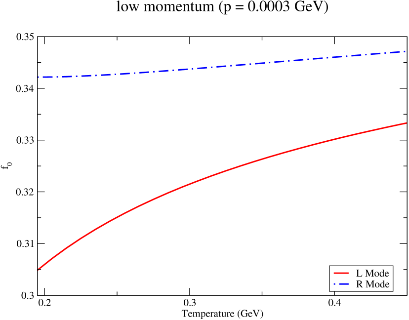
(a)

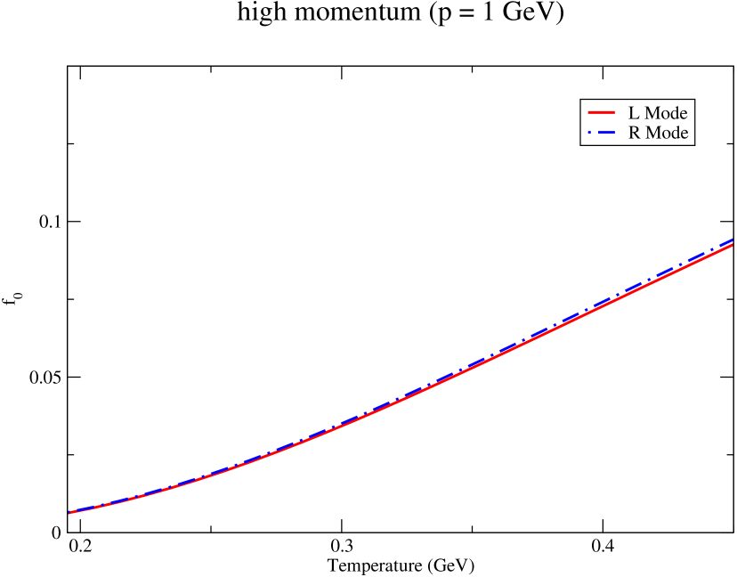
(b)

Figure 2: Variation of distribution function of quark ($f_{0}$) in left- and right-handed mode with temperature, where effective quark mass has been used.

(a)

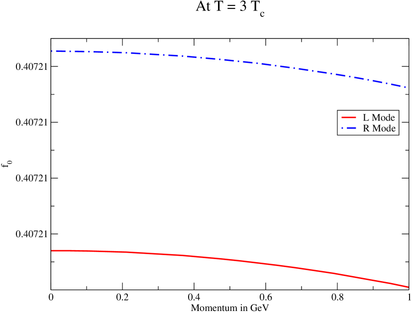
(b)

Figure 3: Variation of distribution function of quark ($f_{0}$) in left- and right-handed mode with momentum, where effective quark mass has been used.

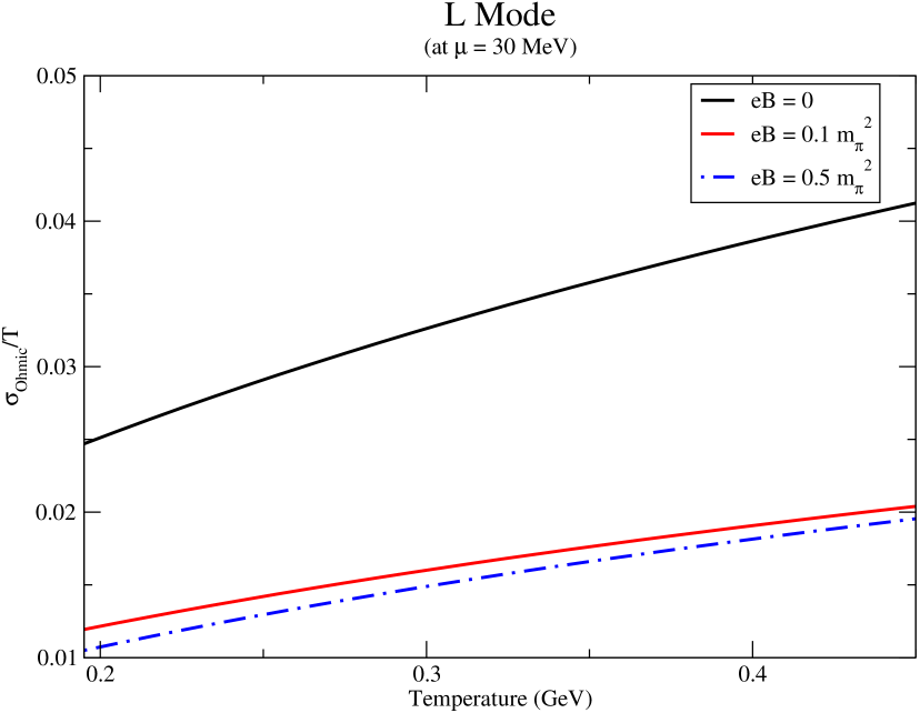
(a)

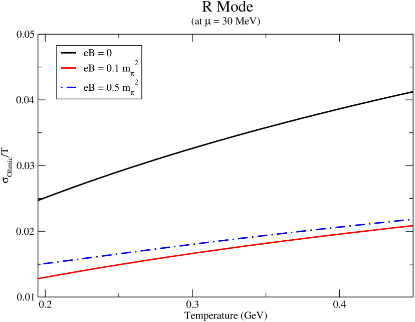
(b)

Figure 4: Variation of $\sigma_{\text{Ohmic}}/T$ for L mode and R mode with temperature at different fixed values of magnetic field.

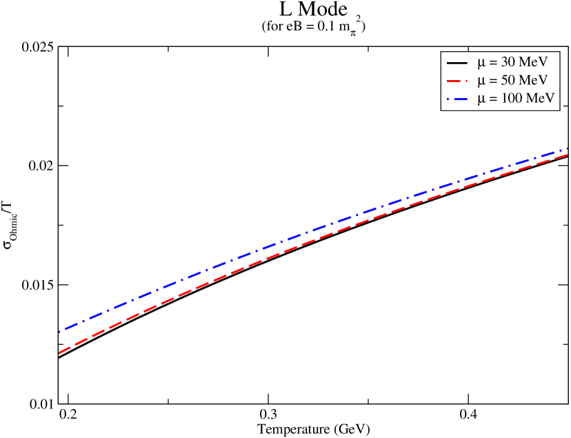
(a)

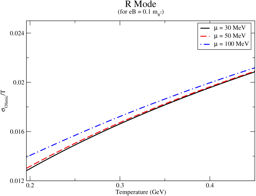
(b)

Figure 5: Variation of $\sigma_{\text{Ohmic}}/T$ for L mode and R mode with temperature at different fixed values of quark chemical potential.

(a)

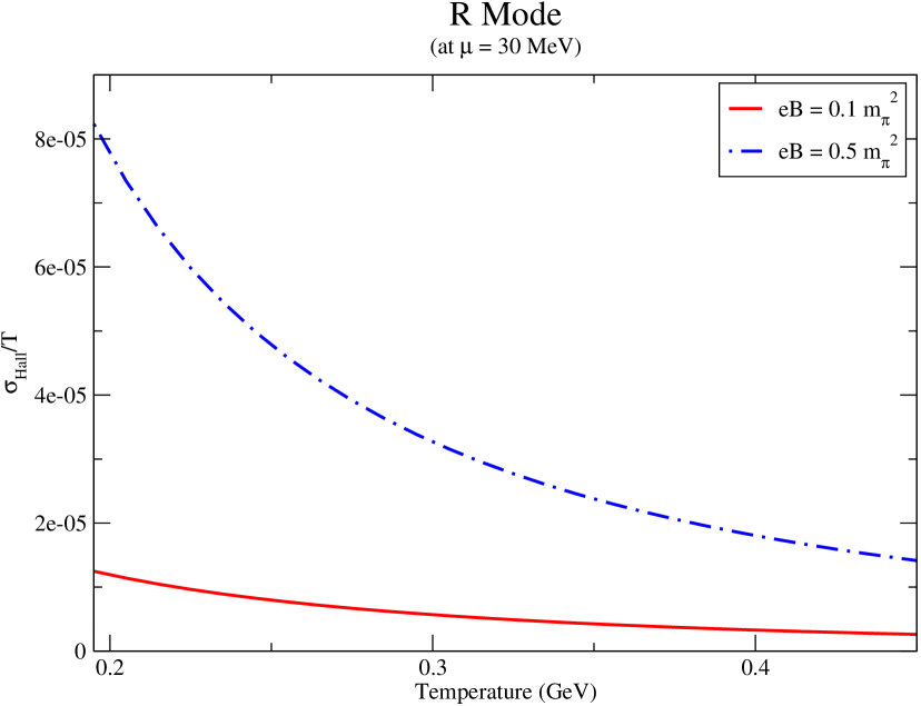
(b)

Figure 6: Variation of $\sigma_{\text{Hall}}/T$ for L mode and R mode with temperature at different fixed values of magnetic field.

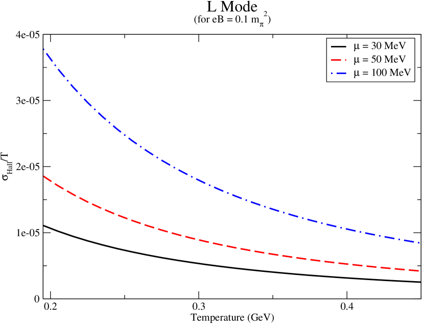
(a)

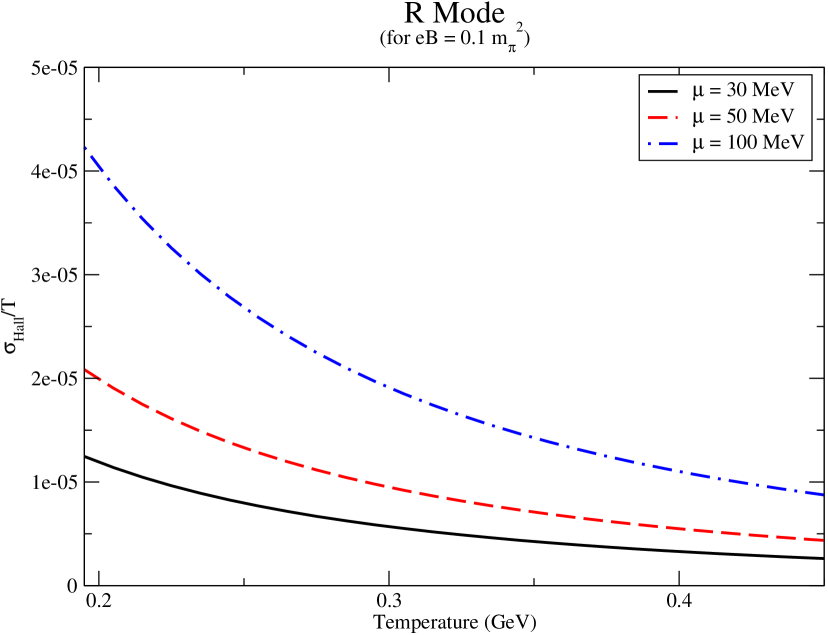
(b)

Figure 7: Variation of $\sigma_{\text{Hall}}/T$ for L mode and R mode with temperature at different fixed values of quark chemical potential.

In Fig.(4), we have shown the variation of ratio of Ohmic conductivity to temperature ($\sigma_{{\text{Ohmic}}}/T$) with respect to temperature for zero and finite magnetic field at non-zero chemical potential ($\mu$=30 MeV). It is evident that the magnitude of $\sigma_{{\text{Ohmic}}}/T$ gets decrease in presence of magnetic field as shown in Fig.(4(a)) and (4(b)). The difference between the magnitude of conductivities for L- and R-mode increases with increase in magnetic field due different effective quark mass for L- and R-mode Eq.(44). This can also be deduced from the plots of distribution function of quark for left-handed and right-handed mode at fixed momentum and temperature shown in Fig.(2) and (3) respectively where $T_{c}\simeq 160MeV$ is the deconfinement temperature from hadron phase to QGP phase. Further, $\sigma_{{\text{Ohmic}}}/T$ for L mode decreases with magnetic field whereas it shows increasing trend for R mode. This behaviour of $\sigma_{{\text{Ohmic}}}/T$ with magnetic field for L and R mode is attributed to the factor $\frac{\tau}{\varepsilon^{2}(1+\omega_{c}^{2}\tau^{2})}$. The thermal mass squared with magnetic field correction for left (right) handed mode is $m_{L(R)}^{2}=m_{th}^{2}\pm 4g^{2}C_{F}M^{2}$, which is found to increase (decreasing) with magnetic field. As this mass appears in the denominator of $\frac{\tau}{\varepsilon^{2}(1+\omega_{c}^{2}\tau^{2})}$ which leads to the decreasing (increasing) behaviour of $\sigma_{{\text{Ohmic}}}/T$ for left (right) handed mode. The increasing behaviour of $\sigma_{\text{Ohmic}}/T$ with temperature for both modes could be due to the Boltzmann factor $\exp(-\varepsilon(p)/T)$ in the distribution function. Fig.(5) shows the variation of normalized Ohmic conductivity at different constant values of quark chemical potential for eB = $0.1m_{\pi}^{2}$, where it increases with increase in quark chemical potential for both modes. With increasing quark chemical potential the Boltzmann factor $\exp(-\mu/T)$ increases due to the higher contribution from quarks than antiquarks. The transverse motion of charged particle under the action of Lorentz force leads to the generation of Hall current. The variation of $\sigma_{{\text{Hall}}}/T$ with temperature for different values of magnetic field at $\mu=30$ MeV is shown in Fig.(6) for both modes. It increases with magnetic field as $\sigma_{{\text{Hall}}}/T$ is proportional to $\omega_{c}$ for the considered range of temperature, chemical potential and magnetic field. The decreasing behaviour of normalized Hall conductivity with temperature is predominantly due to the factor $\omega_{c}\tau$ in the numerator of Eq.(72). $\sigma_{{\text{Hall}}}/T$ for left-handed mode is relatively smaller than right-handed mode as the mass for left mode is comparatively larger than right mode. Hence, we can say that the variation of Ohmic conductivity with magnetic field is affected through the effective mass as shown in Fig.(4), where at $eB=0$, $\sigma_{{\text{Ohmic}}}/T$ has relatively higher magnitude. At $eB=0$, Hall conductivity vanishes and its behaviour with magnetic field is affected through the direct dependence on $q_{f}B$ in the numerator of Eq.(72). Similar to Ohmic conductivity, Hall conductivity also increases with quark chemical potential for L- and R-mode as shown in Fig.(7). At zero chemical potential, number of quarks and antiquarks are same and their contribution to the Hall current is same but opposite in direction. So, the net Hall current vanishes at zero chemical potential and can be explicitly seen in Eq. (72).

V.B Thermal and Hall-type thermal conductivity

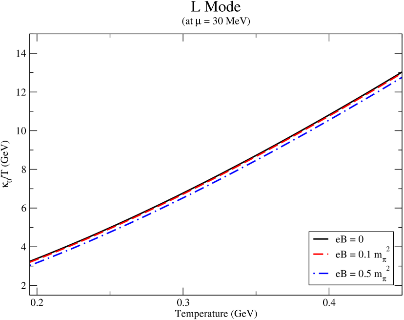
(a)

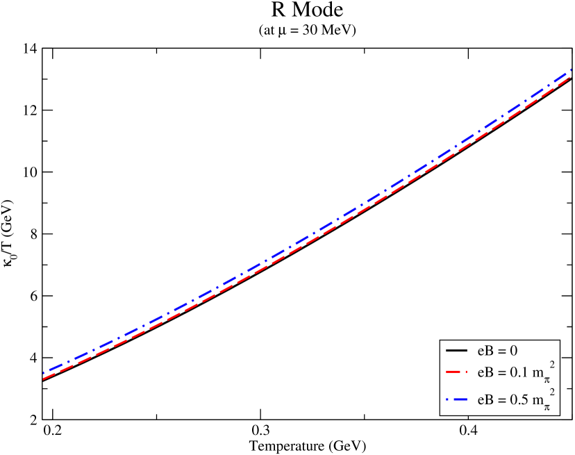
(b)

Figure 8: Variation of $\kappa_{0}/T$ for L and R mode with temperature at different fixed values of magnetic field.

(a)

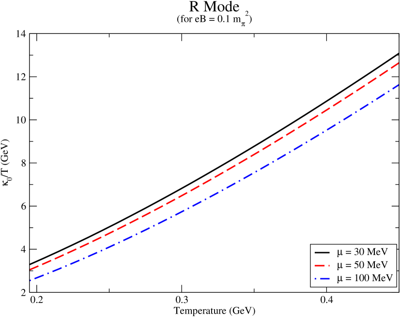
(b)

Figure 9: Variation of $\kappa_{0}/T$ for L and R mode with temperature at different fixed values of quark chemical potential.

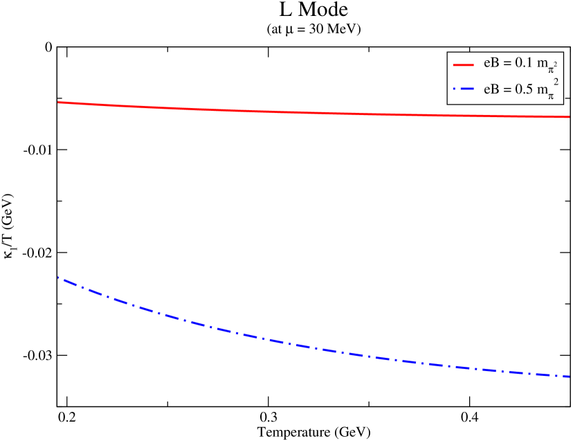
(a)

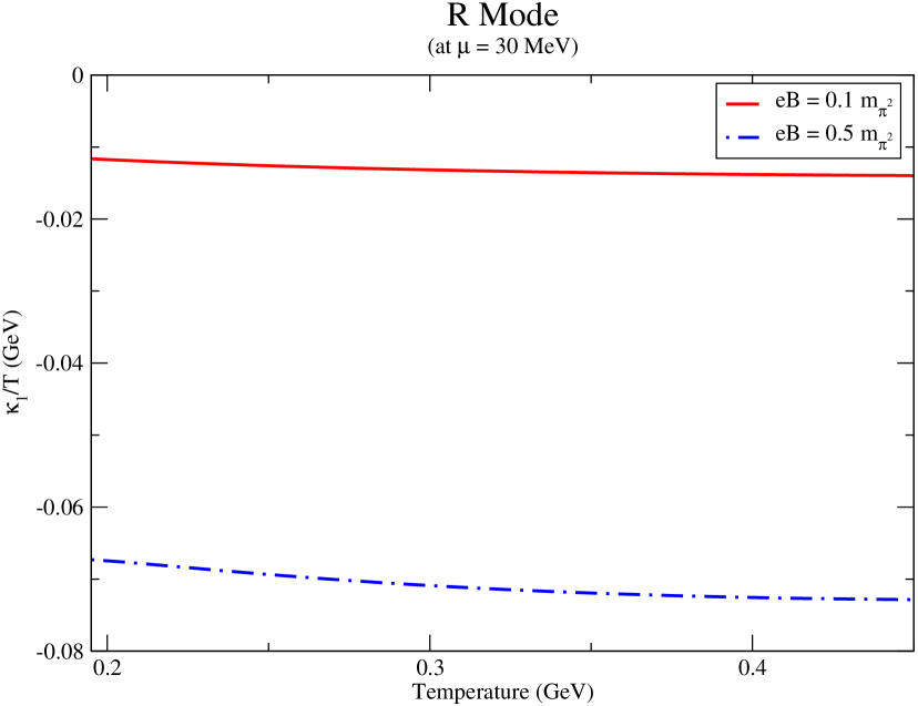
(b)

Figure 10: Variation of $\kappa_{1}/T$ for L and R mode with temperature at different fixed values of magnetic field.

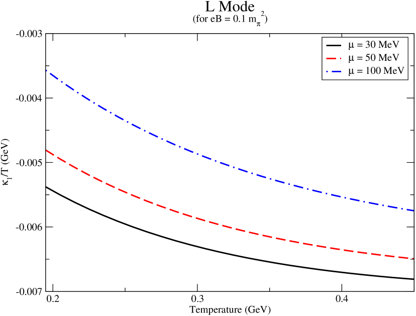
(a)

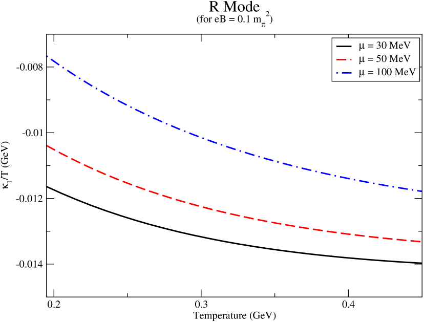
(b)

Figure 11: Variation of $\kappa_{1}/T$ for L and R mode with temperature at different fixed values of quark chemical potential.

Fig.(8) and (9) shows the variation of ratio of thermal conductivity to temperature ($\kappa_{0}/T$) for left and right-handed mode with temperature at different fixed values of magnetic field and quark chemical potential respectively. At zero magnetic field, there would be no lifting of degeneracy and hence we compared $\kappa_{0}/T$ in the absence and presence of magnetic field (with both modes). $\kappa_{0}/T$ increases with temperature for both modes and has approximately the same value at eB = 0.1 $m_{\pi}^{2}$. The increasing behaviour of $\kappa_{0}/T$ with temperature is due to the factor $(\varepsilon-h)^{2}$, $(\varepsilon+h)^{2}$ and distribution function as can be seen from Eq.(119). Further, $\kappa_{0}/T$ for L mode decreases with magnetic field whereas for R mode it increases with magnetic field. The difference between magnitude of thermal conductivity for left- and right-handed mode is again attributed to the different effective quark mass for both modes, similar to the $\sigma_{{\text{Ohmic}}}/T$. Since, $(\varepsilon+h)^{2}$ is higher in magnitude than $(\varepsilon-h)^{2}$ therefore $(\varepsilon+h)^{2}\exp(\mu/T)$ leads to the decreasing behaviour of $\kappa_{0}/T$ with quark chemical potential for both modes. Furthermore, due to the deflected motion of particles under the action of Lorentz force, there is generation of Hall component of thermal conductivity ($\kappa_{1}$) in a direction perpendicular to both the magnetic field and initial thermal driving force. The variation of $\kappa_{1}/T$ with temperature at different fixed values of magnetic field and quark chemical potential is shown in Fig.(10) and (11) respectively for both modes. Considering the absolute value of the ratio $(\kappa_{1}/T)$, we infer that $(\kappa_{1}/T)$ increases with temperature and magnetic field. The increasing behaviour with temperature is due to the $(\varepsilon+h)^{2}$ factor in the numerator of Eq.(111). Moreover, the direct dependence on magnetic field leads to the amplification of Hall-type thermal conductivity with magnetic field. Further, $\kappa_{1}/T$ decreases with quark chemical potential and will not vanish for $\mu=0$ due to the unequal contribution from quarks and anti-quarks in the same direction. We can also infer that the behaviour of longitudinal thermal conductivity with magnetic field is affected through the effective quark mass for both modes whereas Hall type thermal conductivity is affected through direct dependence on magnetic field as could be seen in Eq.(111). $\kappa_{1}/T$ is comparatively smaller in magnitude than $\kappa_{0}/T$, similar to the charge transport.

V.C Knudsen Number

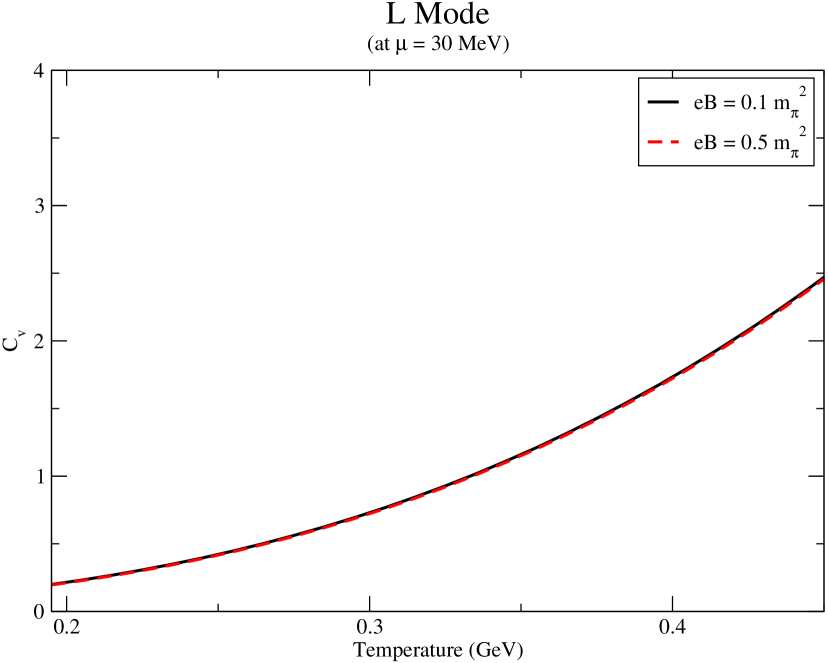
(a)

(b)

Figure 12: Variation $C_{v}$ for L and R mode with temperature where effective quark mass has been used for both modes.

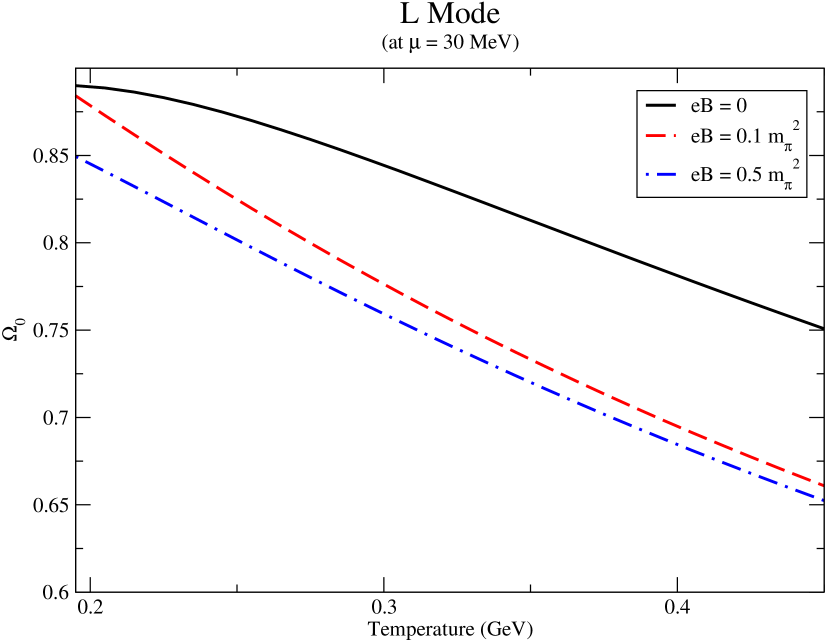
(a)

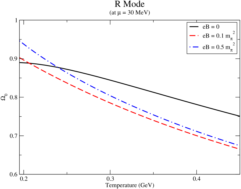
(b)

Figure 13: Variation of Knudsen number ($\Omega_{0}$) for L- and R-mode with temperature at different fixed values of magnetic field.

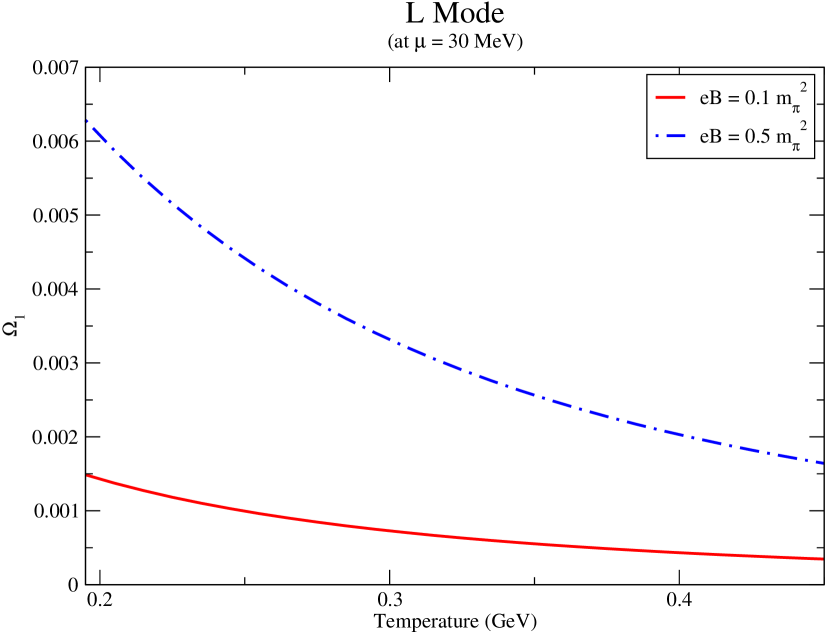
(a)

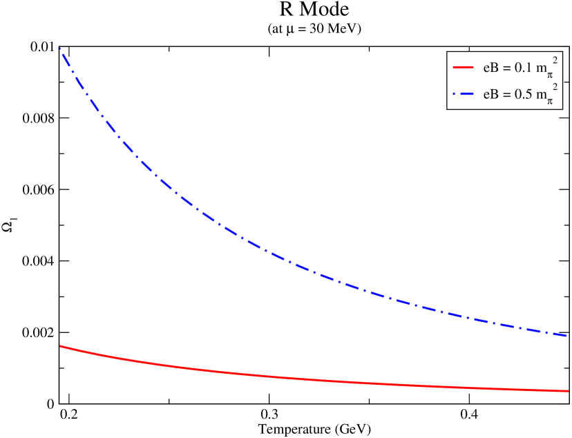
(b)

Figure 14: Variation of Knudsen number ($\Omega_{1}$) for L- and R-mode with temperature at different fixed values of magnetic field.

The applicability of ideal hydrodynamic requires local thermal equilibration. The degree of thermalization in fluid produced in heavy ion collision can be characterized by dimensionless parameter which is termed as Knudsen number ($\Omega$), which is the ratio of microscopic length scale (mean free path) to the macroscopic length scale (characteristic length scale) of the system [88]. The mean free path ($\lambda$) is identified as $3\kappa/(\mathrm{v}C_{v})$ with $\mathrm{v}$ and $C_{v}$ as relative velocity and specific heat at constant volume respectively. Knudsen number can be recast as

$$\Omega=\frac{3\kappa}{\text{v}C_{v}L},$$ (120)

where we have taken $\text{v}\simeq 1$, $L$=4 fm. $C_{v}$ is evaluated from the temperature gradient of energy density, i.e., $C_{v}=\partial(u_{\alpha}T^{\alpha\beta}u_{\beta})/\partial T$. The small value of Knudsen number implies the large number of collisions which bring the system back to local equilibrium. The behaviour of $\Omega_{0}$ (associated to $\kappa_{0}$ and $\kappa_{g}$) and $\Omega_{1}$ (associated to $\kappa_{1}$) with magnetic field is found to be closely related to behaviour of $\kappa_{0}$ and $\kappa_{1}$ for both modes. As we can see that effect of magnetic field on $C_{v}$ is not so much pronounced as shown in Fig.(12(a)) and (12(b)). $\Omega_{0}$ decreases with magnetic field for L-mode whereas increases with magnetic field for R-mode as shown in Fig.(13), similar to the $\kappa_{0}/T$. Moreover, $\Omega_{1}$ shows the increasing trend with magnetic field as shown in Fig.(14), similar to the trends followed by $\kappa_{1}/T$ (taking the absolute value of $\kappa_{1}$). Knudsen number ($\Omega_{0}$ and $\Omega_{1}$) is found to be less than unity for both modes in presence of weak magnetic field at $\mu=30MeV$, thus ensures the system to be in thermal equilibrium.

V.D Wiedemann-Franz law

The interplay between charge and heat transport coefficients can be understood via Wiedemann-Franz law. The temperature behaviour of Lorenz number ($\kappa_{0}/\sigma_{\text{Ohmic}}T$) (for L- and R-mode) and Hall-Lorenz number ($\kappa_{1}/\sigma_{\text{Hall}}T$) (for L- and R-mode) for eB = 0.1$m_{\pi}^{2}$, 0.5 $m_{\pi}^{2}$ at $\mu$= 30 MeV is plotted in Fig.(15) and (17). Lorenz number in absence of magnetic field at finite chemical potential is shown in Fig.(16). Since, Lorenz and Hall-Lorenz number is larger than unity implying that the effect of thermal transport coefficient is more pronounced than charge transport coefficient, hence suggesting that hot QCD matter is good conductor of heat than charge. It is evident that Lorenz and Hall Lorenz number is not constant with temperature. Lorenz number for L-mode increases with magnetic field whereas for R-mode decreases with magnetic field. For L-mode, Lorenz number shows the increasing trend with temperature for $eB=0.1m_{\pi}^{2}$ whereas with further increase the magnetic field it start decreasing with temperature. This opposite behaviour with temperature is due to the difference in the increment of the ratio $(\kappa_{0}/\sigma_{{\text{Ohmic}}})$ at $eB=0.1m_{\pi}^{2},0.5m_{\pi}^{2}$. Hall Lorenz number for L-mode increases with magnetic field whereas that for R-mode, it decreases with magnetic field similar to the previous case as shown in Fig.(15). It increases with temperature for both modes. Here, the behaviour of Lorenz number is found to be in contrast with the case of metals where it is roughly same in Drude model at temperature 273 K and 373 K [38]. Therefore, violation of Wiedemann-Franz law is observed.

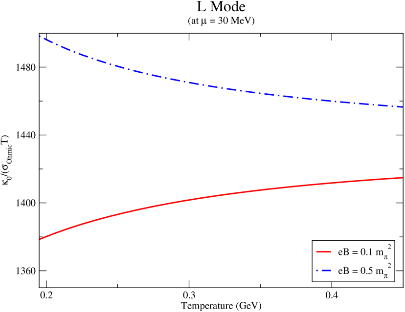
(a)

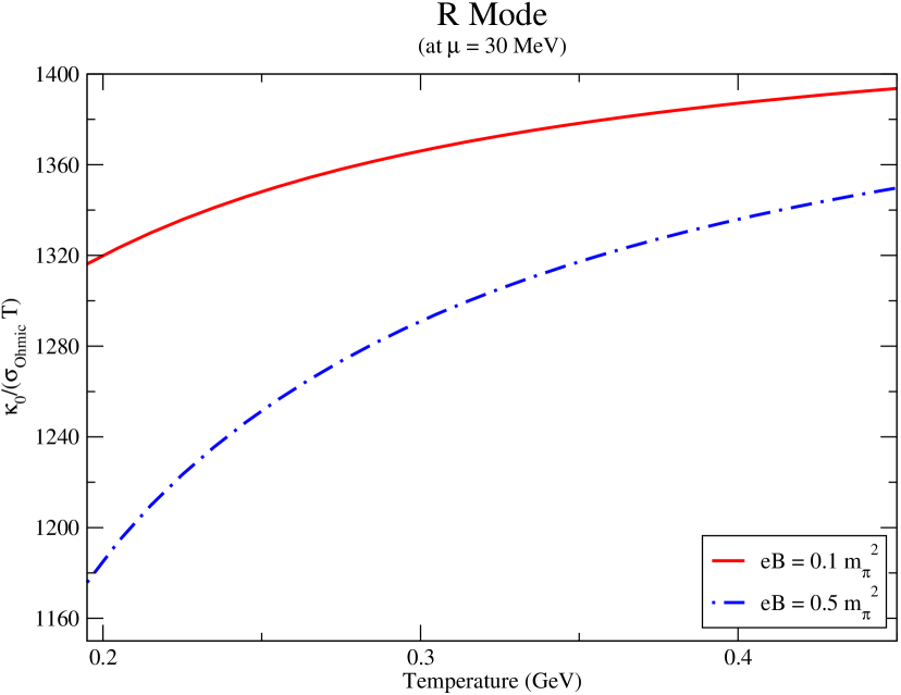
(b)

Figure 15: Variation of Lorenz number for L- and R-mode with temperature at different fixed values of magnetic field.

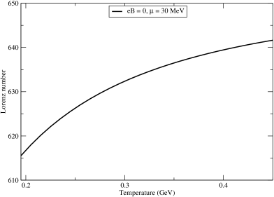
Figure 16: Variation of Lorenz number with temperature for zero magnetic field at finite chemical potential.

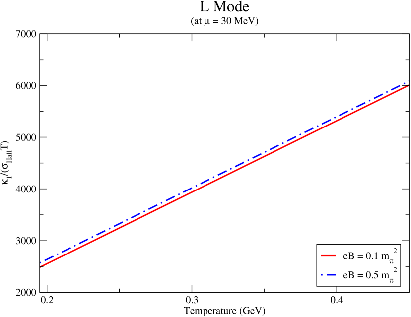
(a)

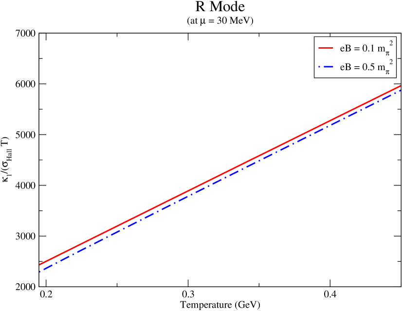
(b)

Figure 17: Variation of Hall Lorenz number for L- and R-mode with temperature at different fixed values of magnetic field.

VI CONCLUSION

In this work, we have studied the charge and heat transport coefficients in hot QCD matter in presence of weak magnetic field at finite chemical potential, where interactions have been incorporated through effective masses using quasiparticle description. In weak magnetic field, we have found that the left- and right-handed chiral modes of quarks get separated due to difference in their mass and become non-degenerate contrary to the strong magnetic field case. Another consequence of weak magnetic field also came into light in transport phenomena as generation of Hall effect. Transport coefficients adopts the tensorial structure where we get the non-vanishing transverse responses. The diagonal elements of tensor structure of transport coefficients gives longitudinal conductivity whereas off-diagonal elements represents their Hall counterparts. We have calculated the transport coefficients using the effective mass of quarks for left- (L) and right-handed (R) chiral modes separately and studied the effect of magnetic field and quark chemical potential on transport coefficients for both modes. We studied the variation of $\sigma_{{\text{Ohmic}}}/T$ and $\sigma_{{\text{Hall}}}/T$ for L- and R- modes at different values of magnetic field and quark chemical potential with temperature. $\sigma_{{\text{Ohmic}}}/T$ for L-mode decreases with magnetic field whereas it increases with magnetic field for R-mode. The opposite behaviour with magnetic field for L- and R-mode in Ohmic conductivity is due to different values of effective quark mass for both modes. On the other hand, $\sigma_{{\text{Hall}}}/T$ for both modes increases with magnetic field. This is due the to direct dependence of magnetic field on Hall conductivity. Additionally, both the conductivities for L- and R-mode positively amplifies with quark chemical potential. Hall conductivity vanishes at zero quark chemical potential due to equal and opposite contribution of quarks and anti-quarks. Analogous to Ohmic and Hall conductivity, we have studied the thermal and Hall-type thermal conductivity for both modes. Since, gluons are not affected by magnetic field therefore thermal conductivity due to gluons is incorporated in longitudinal thermal conductivity. The Hall-type thermal conductivity is the manifestation of transverse temperature gradient under the action of Lorentz force. $\kappa_{0}/T$ for L- and R-mode shows mutually opposite behaviour with magnetic field which is again due to the different effective quark masses for left- and right-handed mode. $\kappa_{1}/T$ increases with magnetic field for both the modes similar to the Hall conductivity in charge transport. Both the conductivities record a drop in their values with increasing quark chemical potential. Moreover, $\kappa_{1}$ does not vanish at zero quark chemical potential due to the unequal contribution from quarks and anti-quarks in the same direction. In application of aforementioned conductivities, we have investigated the equilibrium property through Knudsen number ($\Omega_{0}$ and $\Omega_{1}$) where it is found to be less than unity ensuring the system to be in thermal equilibrium. The variation of Knudsen number with magnetic field is found to be closely related to the thermal and Hall-type thermal conductivity, as the specific heat at constant volume doesn’t show significant change with magnetic field. Further, the relative behaviour of charge and heat transport coefficients has been studied via Wiedemann-Franz law where Lorenz and Hall Lorenz number are found to be greater than unity, hence depicting that hot QCD matter is good conductor of heat. Moreover, Lorenz and Hall Lorenz number increases with magnetic field for L-mode and decreases with magnetic field for R-mode. Lorenz number for L-mode (at eB = 0.1 m${}_{\pi}^{2}$) and for R-mode (at eB = 0.1 m${}_{\pi}^{2}$, 0.5 m${}_{\pi}^{2}$) increases with temperature. As we further increase the magnetic field, Lorenz number for L-mode shows a decreasing trend with temperature. Since, Lorenz and Hall Lorenz number are not constant with temperature, thereby violating the Wiedemann-Franz law.

Appendix A CALCULATION OF STRUCTURE FUNCTIONS

Here, we will show the computation of structure functions from Eq.(18) to (21) in one-loop order for hot and weakly magnetized medium under HTL approximation. Since, trace of odd number of gamma matrices is zero, the Eq.(18) can be written as

$$\mathcal{A}=\frac{1}{4}\frac{\text{Tr}(\Sigma_{0}\not{P})-(P.u)\text{Tr}(\Sigma_{0}\not{u})}{(P.u)^{2}-P^{2}},$$ (A.121)

where,

$$\Sigma_{0}=g^{2}C_{F}T\sum_{n}\int\frac{d^{3}k}{(2\pi)^{3}}\gamma_{\mu}\frac{\not{K}}{K^{2}-m_{f}^{2}}\gamma^{\mu}\frac{1}{(P-K)^{2}}.$$ (A.122)

Using the following two traces:

$$\text{Tr}\left[\gamma_{\mu}\not{K}\gamma^{\mu}\not{P}\right]=-8K.P,$$ (A.123)

$$\text{Tr}\left[\gamma_{\mu}\not{K}\gamma^{\mu}\not{u}\right]=-8K.u,$$ (A.124)

we obtain,

$$\mathcal{A}(P)=\frac{1}{4\bf{|p|}^{2}}g^{2}C_{F}\left[I_{1}(P)+I_{2}(P)\right],$$ (A.126)

where $(P.u)^{2}-P^{2}=\bf{|p|}^{2}$. We will use the frequency sum to evaluate $I_{1}(P)$ and $I_{2}(P)$ with $k_{0}=i\omega_{n}$, $p_{0}=i\omega$, $E_{1}=\sqrt{k^{2}+m_{f0}^{2}}$ and $E_{2}=\sqrt{(p-k)^{2}}$. The frequency sum for fermion-boson case is [68]

$$T\sum_{n}\tilde{\Delta}_{s1}(i\omega_{n},E_{1})\Delta_{s2}(i(\omega-\omega_{n}),E_{2})=\sum_{s1,s2=\pm 1}-\frac{s_{1}s_{2}}{4E_{1}E_{2}}\frac{\left(1-\tilde{f}(s_{1}E_{1})+f(s_{2}E_{2})\right)}{i\omega-s_{1}E_{1}-s_{2}E_{2}}.$$ (A.127)

The leading $T^{2}$ behaviour will come from $s_{1}=-s_{2}=1$ with $E_{1}\approx k$ and $E_{2}=|\bf{p-k}|$. Defining light-like four-vector $\hat{K}=(-i,\bf{\hat{k}})$ and $\hat{K}^{\prime}=(-i,\bf{-\hat{k}})$, we have,

$$i\omega+E_{1}-E_{2}\simeq i\omega+{\bf{p.\hat{k}}}=P.\hat{K},$$ (A.128)

$$i\omega-E_{1}+E_{2}\simeq i\omega-{\bf{p.\hat{k}}}=P.\hat{K^{\prime}},$$ (A.129)

and using the angular integration under HTL approximation,

$$\int\frac{d\Omega}{4\pi}\frac{\hat{K}.u}{P.\hat{K}}=\frac{1}{|\bf{p}|}Q_{0}\left(\frac{p_{0}}{|\bf{p}|}\right),$$ (A.130)

we get,

$$\mathcal{A}(p_{0},{|\bf{p}}|)=\frac{m_{th}^{2}}{{|\bf{p}}|^{2}}Q_{1}\left(\frac{p_{0}}{|\bf{p}|}\right).$$ (A.131)

Similarly, structure function $\mathcal{B}$ can be evaluated as

$$\mathcal{B}(p_{0},{|\bf{p}}|)=-\frac{m_{th}^{2}}{{|\bf{p}|}^{2}}\left[\frac{p_{0}}{|\bf{p}|}Q_{1}\left(\frac{p_{0}}{|\bf{p}|}\right)-Q_{0}\left(\frac{p_{0}}{|\bf{p}|}\right)\right].$$ (A.132)

Using Eq.(II) in (20) and (21), where the contribution from $\Sigma_{0}$ vanishes due to the trace of odd no. of gamma matrices and we get the non-vanishing contribution form $\Sigma_{1}$ only and hence we get,

$$\mathcal{C}\left(p_{0},{\bf{|p|}}\right)=-\frac{1}{4}\text{Tr}(\gamma_{5}\Sigma_{1}\not{u}),$$ (A.133)

$$\mathcal{D}\left(p_{0},{\bf{|p|}}\right)=\frac{1}{4}\text{Tr}(\gamma_{5}\Sigma_{1}\not{b}).$$ (A.134)

Using the following two traces

$$\text{Tr}\left[\gamma_{5}\gamma_{\mu}\gamma_{5}\left[(K.b)\not{u}-(K.u)\not{b}\right]\gamma^{\mu}\not{u}\right]=8(K.b),$$ (A.135)

$$\text{Tr}\left[\gamma_{5}\gamma_{\mu}\gamma_{5}\left[(K.b)\not{u}-(K.u)\not{b}\right]\gamma^{\mu}\not{b}\right]=8(K.u),$$ (A.136)

we obtain,

$$\mathcal{C}=\frac{g^{2}C_{F}|q_{f}B|}{4}T\sum_{n}\int\frac{d^{3}k}{(2\pi)^{3}}\frac{8(K.b)}{(K^{2}-m_{f0}^{2})^{2}(P-K)^{2}},$$ (A.137)

$$\mathcal{D}=-\frac{g^{2}C_{F}|q_{f}B|}{4}T\sum_{n}\int\frac{d^{3}k}{(2\pi)^{3}}\frac{8(K.u)}{(K^{2}-m_{f0}^{2})^{2}(P-K)^{2}},$$ (A.138)

which in turn requires the calculation of frequency sum [89]

$$Y=T\sum_{n}\Delta_{F}^{2}(K)\Delta_{B}(P-K),$$ (A.139)

$$=\left(\frac{-\partial}{\partial m_{f0}^{2}}\right)T\sum_{n}\Delta_{F}(K)\Delta_{B}(P-K),$$

where,

$$T\sum_{n}\Delta_{F}(K)\Delta_{B}(P-K)=\sum_{s1,s2=\pm 1}-\frac{s_{1}s_{2}}{4E_{1}E_{2}}\frac{\left(1-\tilde{f}(s_{1}E_{1})+f(s_{2}E_{2})\right)}{i\omega-s_{1}E_{1}-s_{2}E_{2}}.$$ (A.140)

For $s_{1}=-s_{2}=1$, we get,

$$\mathcal{C}=\frac{4g^{2}C_{F}|q_{f}B|}{16\pi^{2}}\left(\frac{\pi T}{2m_{f0}}-\text{ln}2+\frac{7\mu^{2}\zeta(3)}{8\pi^{2}T^{2}}\right)\left[\frac{-p_{z}}{{\bf|p|}^{2}}Q_{1}\left(\frac{p_{0}}{|\bf{p}|}\right)\right],$$ (A.141)

$$\mathcal{D}=-\frac{4g^{2}C_{F}|q_{f}B|}{16\pi^{2}}\left(\frac{\pi T}{2m_{f0}}-\text{ln}2+\frac{7\mu^{2}\zeta(3)}{8\pi^{2}T^{2}}\right)\left[\frac{1}{{\bf|p|}}Q_{0}\left(\frac{p_{0}}{|\bf{p}|}\right)\right].$$ (A.142)

References

- [1] M. Gyulassy and L. McLerran, Nuclear Physics A 750 (2005) 30–63.
- [2] V. V. Skokov, A. Yu. Illarionov, and V. D. Toneev, Int. J. Mod. Phys. A 24, 5925 (2009).
- [3] D. E. Kharzeev, L. D. McLerran, and H. J. Warringa, Nuclear Physics A 803 (2008) 227–253.
- [4] K. Fukushima, D. E. Kharzeev, and H. J. Warringa, Phys. Rev. Lett. 104, 212001 (2010).
- [5] K. Tuchin, Phys. Rev. C 88, 024911 (2013).
- [6] K. Tuchin, Phys. Rev. C 93, 014905 (2016).
- [7] L. McLerran and V. Skokov, Nucl. Phys. A 929, (2014) 184-190.
- [8] E. Stewart and K. Tuchin, Phys. Rev. C 97, 044906 (2018).
- [9] A. Das, S. S. Dave, P. S. Saumia, and A. M. Srivastava, Phys. Rev. C 96, 034902 (2017).
- [10] K. Tuchin, Phys. Rev. C 83, 017901 (2011).
- [11] M. Greif, C. Greiner, and G. S. Denicol, Phys. Rev. D 93, 096012 (2016).
- [12] M. Greif, I. Bouras, C. Greiner, and Z. Xu, Phys. Rev. D 90, 094014 (2014).
- [13] A. Puglisi, S. Plumari, and V. Greco, Phys. Lett. B 751, 326-330 (2015).
- [14] A. Puglisi, S. Plumari, and V. Greco, Phys. Rev. D 90, 114009 (2014).
- [15] W. Cassing, O. Linnyk, T. Steinert, and V. Ozvenchuk, Phys. Rev. Lett. 110, 182301 (2013).
- [16] T. Steinert and W. Cassing, Phys. Rev. C 89, 035203 (2014).
- [17] S. Rath and B. K. Patra, Phys. Rev. D 100, 016009 (2019).
- [18] D. Dey and B. K. Patra, Phys. Rev. D 102, 096011 (2020).
- [19] S. Rath and B. K. Patra, J. High Energy Phys. 12 (2017) 098.
- [20] B. Karmakar, R. Ghosh, A. Bandyopadhyay, N. Haque, and M.G. Mustafa, Phys. Rev. D 99, 094002 (2019).
- [21] K. Tuchin, Phys. Rev. C 88, 024910 (2013).
- [22] A. Peshier and M. H. Thoma, Phys. Rev. Lett. 84, 841 (2000).
- [23] K.A. Mamo, J. High Energy Phys. 1308 (2013) 083.
- [24] U. Heinz1 and R. Snellings, Annu. Rev. Nucl. Part. Sci. 63, 123 (2013).
- [25] B. Schenke, S. Jeon, and C. Gale, Phys. Rev. C 82, 014903 (2010).
- [26] H. Niemi, G. S. Denicol, P. Huovinen, E. Molnar, and D. H. Rischke, Phys. Rev. Lett. 106, 212302 (2011).
- [27] P. K. Kovtun, D. T. Son, and A. O. Starinets, Phys. Rev. Lett. 94, 111601 (2005).
- [28] P. Romatschke and U. Romatschke, Phys. Rev. Lett. 99, 172301 (2007).
- [29] D. Teaney, J. Lauret, and E. V. Shuryak, Phys. Rev. Lett. 86, 4783 (2001).
- [30] P. Huovinen, P. F. Kolb, U. Heinz, P. V. Ruuskanen, and S. A. Voloshin, Phys. Lett. B 503, (2001) 58-64.
- [31] R. Baier, P. Romatschke, and U. A. Wiedemann, Phys. Rev. C 73, 064903 (2006).
- [32] U. Heinz, H. Song, and A. K. Chaudhuri, Phys. Rev. C 73, 034904 (2006).
- [33] G. S. Denicol et al., Phys. Rev. D 89, 074005 (2014).
- [34] S. Ghosh, Int. J. Mod. Phys. E 24, 1550058 (2015).
- [35] G. Kadam, H. Mishra, and L. Thakur, Phys. Rev. D 98, 114001 (2018).
- [36] K. Fukushima, D. E. Kharzeev, and H. J. Warringa, Phys. Rev. D 78, 074033 (2008).
- [37] K. Haglin, C. Gale, and V. Emel’yanov, Phys. Rev. D 47, 973 (1993).
- [38] Neil W. Ashcroft, N. David Mermin, Solid State Physics (Saunders College Publishing, 1976.)
- [39] A. Principi, and G. Vignale, Phys. Rev. Lett. 115, 056603 (2015).
- [40] R. W. Hill, C. Proust, L. Taillefer, P. Fournier, and R. L. Greene, Nature (London) 414, 711-715 (2001).
- [41] A. Garg, D. Rasch, E. Shimshoni, and A. Rosch, Phys. Rev. Lett. 103, 096402 (2009).
- [42] S. Mitra, and V. Chandra, Phys. Rev. D 96, 094003 (2017).
- [43] R. Rath, et al., Eur. Phys. J. A 55, 125 (2019).
- [44] K. Fukushima, K. Hattori, H.-Ung Yee, and Y. Yin, Phys. Rev. D 93, 074028 (2016).
- [45] R. Marty, E. Bratkovskaya, W. Cassing, J. Aichelin, and H. Berrehrah, Phys. Rev. C 88, 045204 (2013).
- [46] R. Lang, N. Kaiser, and W. Weise, Eur. Phys. J. A 51, 127 (2015).
- [47] S. Ghosh, F. E. Serna, A. Abhishek, G. Krein, and H. Mishra, Phys. Rev. D 99, 014004 (2019).
- [48] A. Wiranata, and M. Prakash, Phys. Rev. C 85, 054908 (2012).
- [49] S. Plumari, A. Puglisi, F. Scardina, and V. Greco, Phys. Rev. C 86, 054902 (2012).
- [50] S. Mitra, and V. Chandra, Phys. Rev. D 94, 034025 (2016).
- [51] S. Ghosh, Int. J. Mod. Phys. A 29, 1450054 (2014).
- [52] A. Harutyunyan, D. H. Rischke, and A. Sedrakian, Phys. Rev. D 95, 114021 (2017).
- [53] N. Demir, and A. Wiranata, J. Phys. Conf. Ser. 535, 012018 (2014).
- [54] S. Satapathy, S. Ghosh, and S. Ghosh, Phys. Rev. D 104, 056030 (2021).
- [55] M. Kurian, and V. Chandra, Phys. Rev. D 97, 116008 (2018).
- [56] M. Kurian, and V. Chandra, Phys. Rev. D 96, 114026 (2017).
- [57] M. Kurian, Phys. Rev. D 102, 014041 (2020).
- [58] K. K. Gowthama, M. Kurian, and V. Chandra, Phys. Rev. D 103, 074017 (2021).
- [59] S. Gupta, Phys. Lett. B 597, 57-62 (2004).
- [60] G. Aarts, et al., JHEP 02, 186 (2015).
- [61] H.-T. Ding, O. Kaczmarek, and F. Meyer, Phys. Rev. D 94, 034504 (2016).
- [62] S. Rath, and B. K. Patra, Eur. Phys. J. C 80, 747 (2020).
- [63] S. A. Khan, and B. K. Patra, Phys. Rev. D 104, 054024 (2021).
- [64] A. Das, H. Mishra, and R. K. Mohapatra, Phys. Rev. D 101, 034027 (2020).
- [65] L. Thakur and P. K. Srivastava, Phys. Rev. D 100, 076016 (2019).
- [66] A. Das, A. Bandyopadhyay, P. K. Roy and, M. G. Mustafa, Phys. Rev. D 97, 034024 (2018).
- [67] H. A. Weldon, Phys. Rev. D 26, 2789 (1982).
- [68] M. Le Bellac, Thermal Field Theory (Cambridge University Press, Cambridge, 1996).
- [69] A. Ayala, C. A. Dominguez, S. Hernandez-Ortiz, L. A. Hernandez, M. Loewe, D. Manreza Paret, and R. Zamora, Phys. Rev. D 98, 031501(R) (2018).
- [70] J-P. Blaizot, and E. Iancu, Phys.Rept. 359 (2002) 355-528.
- [71] V. M. Bannur, , J. High Energy Phys. 09 (2007) 046.
- [72] J. Schwinger, Phys. Rev. 82, 664 (1951).
- [73] T. Chyi, et al., Phys. Rev. D 62, 105014 (2000).
- [74] A. Bandyopadhyay, B. Karmakar, N. Haque, and M. G. Mustafa, Phys. Rev. D 100, 034031 (2019).
- [75] L. D. Landau, E. M. Lifshitz, Course of Theoretical Physics, Volume 10, Physical Kinetics (Pergamon International Library, 1981).
- [76] B. Feng, Phys. Rev. D 96, 036009 (2017).
- [77] A. Hosoya and K. Kajantie, Nucl. Phys. B250, 666 (1985).
- [78] H. Berrehrah, E. Bratkovskaya, W. Cassing, P. B. Gossiaux, J. Aichelin, and M. Bleicher, Phys. Rev. C 89, 054901 (2014) .
- [79] M. Cheng et al, Phys. Rev. D 77, 014511 (2008).
- [80] C. Schmidt et al, Nucl. Phys. A820, 41C (2009).
- [81] L. L. Zhu and C. B. Yang, Nucl. Phys. A831, 49 (2009).
- [82] S. Groot, W. van Leeuwen, and van Weert Ch. G, Relativistic Kinetic Theory (Elsevier North-Holland, New York, 1980).
- [83] L. D. Landau, E. M. Lifshitz, Course of Theoretical Physics, Volume 6, Fluid Mechanics (Pergamon Books Ltd., 1987).
- [84] M. Greif, F. Reining, I. Bouras, G. S. Denicol, Z. Xu, and C. Greiner, Phys. Rev. E 87, 033019 (2013).
- [85] W. Israel and J. M. Stewart, Ann. Phys. 118 (1979) 341.
- [86] A. Haug, Theoretical Solid State Physics, Volume 2 (Pergamon Press Ltd., 1972).
- [87] Charles R. Whitsett, J. Appl. Phys. 32, 2257 (1961).
- [88] A. K. Chaudhuri, Phys. Rev. C 82, 047901 (2010) .
- [89] A. Ayala, J. J. Cobos-Martínez, M. Loewe, M. E. Tejeda-Yeomans, and R. Zamora, Phys. Rev. D 91, 016007 (2015).