A new ranking scheme for modern data and its application to two-sample hypothesis testing

Abstract

Rank-based approaches are among the most popular nonparametric methods for univariate data in tackling statistical problems such as hypothesis testing due to their robustness and effectiveness. However, they are unsatisfactory for more complex data. In the era of big data, high-dimensional and non-Euclidean data, such as networks and images, are ubiquitous and pose challenges for statistical analysis. Existing multivariate ranks such as component-wise, spatial, and depth-based ranks do not apply to non-Euclidean data and have limited performance for high-dimensional data. Instead of dealing with the ranks of observations, we propose two types of ranks applicable to complex data based on a similarity graph constructed on observations: a graph-induced rank defined by the inductive nature of the graph and an overall rank defined by the weight of edges in the graph. To illustrate their utilization, both the new ranks are used to construct test statistics for the two-sample hypothesis testing, which converge to the $\chi_{2}^{2}$ distribution under the permutation null distribution and some mild conditions of the ranks, enabling an easy type-I error control. Simulation studies show that the new method exhibits good power under a wide range of alternatives compared to existing methods. The new test is illustrated on the New York City taxi data for comparing travel patterns in consecutive months and a brain network dataset comparing male and female subjects.

1 Introduction

1.1 Multivariate ranks

High-dimensional and non-Euclidean data have become ubiquitous in the era of big data, such as networks and images, which poses challenges for statistical analysis (Bullmore and Sporns, 2012; Tian et al., 2016; Menafoglio and Secchi, 2017). Parametric approaches are limited when many nuisance parameters need to be estimated. Among the nonparametric methods, rank-based methods are attractive due to their robustness and effectiveness and have been extensively studied for univariate data. However, univariate ranks can not be easily extended to multivariate data due to the lack of natural ordering of the values. The existing extensions of ranks to multivariate data include the component-wise rank (Bickel, 1965; Hallin and Puri, 1995; Puri and Sen, 2013), the spatial rank (Chaudhuri, 1996; Oja, 2010), the depth-based rank (Liu and Singh, 1993; Serfling and Zuo, 2000), the Mahalanobis rank (Hallin and Paindaveine, 2002, 2004, 2006), the metric rank (Pan et al., 2018) and the measure transportation-based rank (Deb and Sen, 2021). Specifically, given $N$ observations $Z_{1},\ldots,Z_{N}\in\mathbb{R}^{d}$:

• The component-wise rank $R_{i}\in\mathbb{R}^{d}$ is the rank vector for each dimension of $Z_{i}$, e.g., $R_{ij}$ is the rank of $Z_{ij}$ among $Z_{1j},\ldots,Z_{Nj}$ for $j=1,\ldots,d$. Since it is defined for each dimension, this rank suffers from correlated covariates and is not invariant to affine transformations.

• The spatial rank function is defined as $R(Z)=\sum_{i=1}^{N}U(Z-Z_{i})/N$ where $U(Z)=Z/\|Z\|$ for $Z\neq\mathbf{0}_{d}$ and $U(\mathbf{0}_{d})=\mathbf{0}_{d}$. The rank is powerful for detecting location differences, but not for distinguishing scale parameters due to the normalizing procedure involved in $U(\cdot)$.

• The depth-based rank measures the centrality of the observations. It depends on the choice of depth function. For example, the Mahalanobis’s depth is defined as ${\rm M}_{h}{\rm D}(Z)=\big{\{}1+(Z-\bar{Z})^{\scriptscriptstyle\sf T}\mathbf{S}^{-1}(Z-\bar{Z})\big{\}}^{-1}\,,$ where $\bar{Z}=\sum_{i=1}^{N}Z_{i}/N$ is the sample mean and $\mathbf{S}$ is the sample covariance matrix, and the Tukey’s depth is defined as ${\rm TD}(Z)=\inf_{\mathcal{X}}\{F_{N}(\mathcal{X}):\mathcal{X}\text{isaclosedhalf-spacecontaining}Z\}$, where $F_{N}$ is the empirical cumulative distribution function. Given a depth function, the depth-based ranks are the ranks of the depth values. The depth ${\rm M}_{h}{\rm D}$ does not work when the dimension is larger than the number of observations. Other depth functions are computationally extensive for high-dimensional data, for example, ${\rm TD}$ has the computational complexity $O(N^{d-1}\log N)$ (Liu, 2017) and the simplicial depth (Liu, 1988) has the computational complexity $O(N^{d}\log N)$ (Afshani et al., 2016).

• The Mahalanobis rank is designed for multivariate one-sample testing, which is defined as the rank of the pseudo-Mahalanobis distance $d(Z,\theta_{0})=(Z-\theta_{0})^{\scriptscriptstyle\sf T}\hat{\boldsymbol}{\Sigma}^{-1}(Z-\theta_{0})$, where $\theta_{0}$ is the location parameter of interest and specified under $H_{0}$, and $\hat{\boldsymbol}{\Sigma}$ is an M-estimator of the covariance matrix due to Tyler (1987). It is powerful for elliptical symmetric distribution but is not robust to heavy-tailed distributions.

• The metric rank measures the difference between two probability distributions. Assume $Z_{1},\dots,Z_{m}\overset{iid}{\sim}F_{X},Z_{m+1},\dots Z_{N}\overset{iid}{\sim}F_{Y}$, and define $nA_{ij}^{X},i,j\in\{1,\ldots,m\}$ be the rank of $d(Z_{i},Z_{j})$ among $\{d(Z_{i},Z_{u}),u=1,\ldots,m\}$ where $d(Z_{i},Z_{j})$ is the distance between $Z_{i}$ and $Z_{j}$, $mA_{ij}^{Y},i,j\in\{1,\ldots,m\}$ be the rank of $d(Z_{i},Z_{j})$ among $\{d(Z_{i},Z_{u}),u=j,m+1,\ldots,N\}$, $nC_{ij}^{X},i,j\in\{m+1,\ldots,N\}$ be the rank of $d(Z_{i},Z_{j})$ among $\{d(Z_{i},Z_{u}),u=1,\ldots,m,j\}$, and $mC_{ij}^{Y},i,j\in\{m+1,\ldots,N\}$ be the rank of $d(Z_{i},Z_{j})$ among $\{d(Z_{i},Z_{u}),u=m+1,\ldots,N\}$. Then the differences $A_{ij}^{X}-A_{ij}^{Y}$ and $C_{ij}^{X}-C_{ij}^{Y}$ are used to compare the two distributions. However, the limiting distribution of the test statistic is not easy to approximate, so a resampling procedure is usually used to obtain the $p$-value.

• The measure transportation-based ranks are defined by the optimization problem

  $$\hat{\sigma}=\arg\min_{\sigma\in\mathcal{S}_{N}}\sum_{i=1}^{N}\|Z_{i}-c_{\sigma(i)}\|^{2}\,,$$

  where $\sigma=(\sigma(1),\ldots,\sigma(N))$ and $\mathcal{S}_{N}$ is the set of all permutations of $\{1,\ldots,N\}$, the multivariate rank vectors $\{c_{1},\ldots,c_{N}\}$ are a sequence of ‘uniform-like’ points in $[0,1]^{d}$ generated from Halton sequences (Hofer, 2009; Hofer and Larcher, 2010). As a result, the rank vector of $Z_{i}$ will be $c_{\hat{\sigma}(i)}$. These ranks are also useful in detecting location differences. However, when the dimension is high, it is difficult to generate ‘uniformly’ distributed rank vectors, which suffers from the curse of dimensionality.

Noticing the limitations of the existing multivariate ranks, we propose ranks that rely on a similarity graph (Section 2). We then build test statistics based on the new ranks for two-sample hypothesis testing (Section 3). The asymptotic properties of the new test statistics are studied (Section 4) and the performance of the new tests is explored through extensive simulation studies (Section 5) and two real data applications (Section 6). The paper concludes with discussions in Section 7.

2 Graph-based ranks

One way of dealing with high-dimensional data is using inter-point distances, which has been shown to capture much information from data (Hall et al., 2005; Biswas and Ghosh, 2014; Angiulli, 2018). However, the distance-based methods suffer from outlier and heavy-tailed distributions. Specifically, many distance-based methods require the existence of some moments for their key theoretical properties to hold (e.g., Li (2018); Guo and Modarres (2020); Chakraborty and Zhang (2021); Zhu and Shao (2021)). On the other hand, the graph-based methods are robust to outlier and heavy-tailed distributions. These methods construct unweighted similarity graphs using the pairwise similarities/distances of the observations, then conduct statistical analysis based on the graphs (e.g., Friedman and Rafsky (1979); Schilling (1986); Henze (1988); Rosenbaum (2005); Chen and Friedman (2017)). We thus want to combine the advantage of both approaches by using more information compared to the graph-based methods while still keeping their robustness and propose the following graph-based ranks.

For two graphs $G_{1}$ and $G_{2}$ with identical vertices, define $G_{1}\cap G_{2}=\emptyset$ if they have no overlapping edges and $G_{1}\cup G_{2}$ as the graph with the same vertex set as them and the edge set their union. Given $N$ independent observations $\{Z_{i}\}_{i=1}^{N}$, and a pre-specified integer $k$, we can construct a sequence of simple similarity graphs $\{G_{l}\}_{l=0}^{k}$ in an inductive way such that $G_{0}$ has no edges and

$$G_{l+1}=G_{l}\cup G_{l+1}^{*}\,\text{with}G_{l+1}^{*}=\arg\max_{G^{\prime}\in\mathcal{G}_{l+1}}\sum_{(i,j)\in G^{\prime}}S(Z_{i},Z_{j})\,,$$

where $\mathcal{G}_{l+1}=\{G^{\prime}\in\mathcal{G}:G^{\prime}\cap G_{l}=\emptyset\}$ and $\mathcal{G}$ is a graph set whose elements satisfy specific user-defined constraints. Here $S(\cdot,\cdot)$ is a similarity measure, for example, $S(Z_{i},Z_{j})=-\|Z_{i}-Z_{j}\|$ for Euclidean data. For other choices of the similarity measures, see Chen and Zhang (2013); Sarkar and Ghosh (2018); Sarkar et al. (2020). Many widely used similarity graphs can be constructed in this way with different constraints, for example,

• $k$-nearest neighbor graph ($k$-NNG): $\mathcal{G}=\{G^{\prime}:$ each vertex $i$ connects to another vertex $j$ $\}$;

• $k$-minimum spanning tree ($k$-MST)(Friedman and Rafsky, 1979): $\mathcal{G}=\{G^{\prime}:$ $G^{\prime}$ is a tree that connects all vertices$\}$;

• $k$-minimum distance non-bipartite pairing ($k$-MDP)(Rosenbaum, 2005): $\mathcal{G}=\{G^{\prime}:$ $G^{\prime}$ is a non-bipartite pairing$\}$;

• $k$-shortest Hamiltonian path ($k$-SHP) (Biswas et al., 2014): $\mathcal{G}=\{G^{\prime}:$ $G^{\prime}$ is a Hamiltonian path$\}$.

Take the $k$-NNG as an example. By definition, $G_{1}$ is the $1$-NNG as the summation of the edges’ similarities is maximized if and only if each vertex connects to its nearest neighbor. With similar arguments, $G_{l+1}^{*}$ is the $(l+1)$th NNG for any $l\geq 1$. Thus, $G_{l+1}$ is the $(l+1)$-NNG. Similarly, for MSTs, $G_{1}$ is the $1$-MST, $G_{l+1}^{*}$ is the $(l+1)$th MST for any $l\geq 1$, and $G_{l+1}$ is the $(l+1)$-MST. An illustration of these graphs is presented in Figure 1.

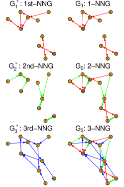
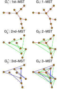
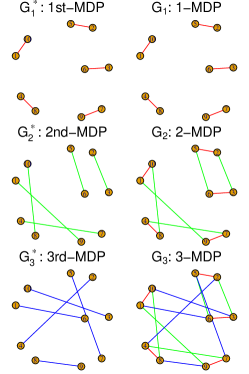
(i) $k$-NNG.	(ii) $k$-MST.	(iii) $k$-MDP.

Figure 1: Examples of different similarity graphs.

With $\{G_{l}\}_{l=1}^{k}$, we define two types of graph-based rank matrices $\mathbf{R}=(R_{ij})_{i,j=1}^{N}\in\mathbb{R}^{N\times N}$ as follows. For an event $A$, $\mathbbm{1}(A)$ is an indicator function that equals to one if event $A$ occurs, and equals to zero otherwise.

• Graph-induced rank

  $$R_{ij}=\sum_{l=1}^{k}\mathbbm{1}\big{(}(i,j)\in G_{l}\big{)}\,.$$ (1)

• Overall rank

  $$R_{ij}={\rm rank}(S(Z_{i},Z_{j}),G_{k})\,,$$ (2)

  where ${\rm rank}(S(Z_{i},Z_{j}),G_{k})$ is the rank of $S(Z_{i},Z_{j})$ among $\{S(Z_{u},Z_{v})\}_{(u,v)\in G_{k}}$ if $(i,j)\in G_{k}$ and is zero if $(i,j)\notin G_{k}$.

Both ranks depend implicitly on $k$, whose choice is discussed in Sections 5 and 7.4. The graph-induced rank $R_{ij}$ is the number of graphs that the edge $(i,j)$ appears in the sequence of graphs $\{G_{1},\ldots,G_{k}\}$. For instance, the graph-induced rank of edges in the $l$th NNG or the $l$th MST will be $k-l+1$ for $k$-NNG and $k$-MST, respectively. The overall rank is the rank of the similarity of edges in the graph $G_{k}$. These graph-based ranks impose more weights on edges with higher similarity, thus incorporating more similarity information than the unweighted graph. In the meantime, the robustness property of the ranks makes the weights less sensitive to outliers compared to the direct utilization of similarity. With these ranks, we are ready to build different test statistics for different problems.

3 A new two-sample test statistic for high-dimensional data and non-Euclidean data

3.1 Two-sample test problem and background

For two independent random samples $X_{1}$, …, $X_{m}\stackrel{{\scriptstyle i.i.d}}{{\sim}}F_{X}$ and $Y_{1}$, …, $Y_{n}\stackrel{{\scriptstyle i.i.d}}{{\sim}}F_{Y}$, we consider the test

$$H_{0}:F_{X}=F_{Y}\quad\text{against}\quad H_{1}:F_{X}\neq F_{Y}\,.$$

For many high-dimensional or non-Euclidean data problems, one has little information on $F_{X}$ and $F_{Y}$, which makes parametric approaches not applicable. A number of nonparametric tests have been proposed for high-dimensional data such as the graph-based tests (Friedman and Rafsky, 1979; Schilling, 1986; Henze, 1988; Rosenbaum, 2005; Chen and Zhang, 2013; Chen and Friedman, 2017; Chen et al., 2018; Zhang and Chen, 2022), the classification-based tests (Hediger et al., 2019; Lopez-Paz and Oquab, 2016; Kim et al., 2021), the interpoint distances-based tests (Székely and Rizzo, 2013; Biswas and Ghosh, 2014; Li, 2018), and the kernel-based tests (Gretton et al., 2008; Eric et al., 2007; Gretton et al., 2009, 2012b; Song and Chen, 2020).

Recently, Pan et al. (2018) introduced Ball Divergence (BD) to measure the difference between the two distributions and proposed a metric rank test procedure. Deb and Sen (2021) proposed to define the multivariate ranks through the theory of measure transportation (Hallin et al., 2021), based on which they built the multivariate rank-based distribution-free nonparametric testing. Both tests can be applied to high-dimensional data and achieve good performance for some useful settings. However, they also lose power under some common alternatives, which will be detailed in Section 5. Besides, even though their asymptotic properties were studied, they were not useful to obtain analytic $p$-value approximations. The random permutation procedure was recommended by the authors to obtain their $p$-values.

3.2 Test statistics on graph-based ranks

Let $Z_{i}=X_{i},i=1,\dots m;Z_{m+j}=Y_{j},j=1,\dots n$ be the pooled samples and $N=m+n$. Let $\mathbf{R}\in\mathbb{R}^{N\times N}$ be the graph-based rank matrix constructed on $\{Z_{i}\}_{i=1}^{N}$ (details see Section 2). We first define two basic quantities based on $\mathbf{R}$:

$$U_{x}=\sum_{i=1}^{m}\sum_{j=1}^{m}R_{ij}\quad{\rm and}\quad U_{y}=\sum_{i=m+1}^{N}\sum_{j=m+1}^{N}R_{ij}\,,$$

which are the within-sample rank sums of sample $X$ and sample $Y$, respectively. We can symmetrize $\mathbf{R}$ by using $\frac{1}{2}(\mathbf{R}+\mathbf{R}^{\scriptscriptstyle\sf T})$. This does not change the values of $U_{x}$ and $U_{y}$ by their definitions; while the derivation for their expectations and variances would be much simpler. With a slight notation abuse, in the following, $\mathbf{R}$ is used for the symmetric version. Before we propose the test statistic, we illustrate the behaviors of $U_{x}$ and $U_{y}$ under different scenarios through toy examples. Here we set $n=m=50$ and consider multivariate Gaussian distribution with dimension $d=100$: (a) null: $F_{X}=F_{Y}=N(\mathbf{0}_{d},\mathbf{I}_{d})$; (b) location alternative: $F_{Y}=N(\mathbf{1}_{d},\mathbf{I}_{d})$; (c) scale alternative: $F_{Y}=N(\mathbf{0}_{d},4\mathbf{I}_{d})$; (d) mixed alternative: $F_{Y}=N(0.5\mathbf{1}_{d},2\mathbf{I}_{d})$.

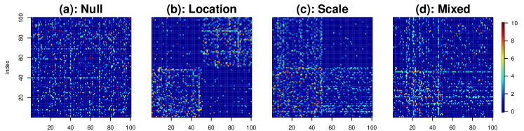
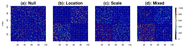
Figure 2: Heatmap of the graph-based rank matrix. Top: graph-induced ranks in $10$-NNG. Bottom: overall ranks in $10$-MDP.

Figure 2 shows the heatmaps of the graph-induced rank matrix in the $10$-NNG and the overall rank matrix in the $10$-MDP. When the two distributions are different in the location parameter, both $U_{x}$ and $U_{y}$ tend to be larger than their corresponding values under the null; while for scale alternative, one of $U_{x}$ and $U_{y}$ tends to be larger while the other one tends to be smaller than their corresponding values under the null. For both location and scale differences, $U_{x}$ and $U_{y}$ will also be different from their values under the null. Thus, $U_{x}$ and $U_{y}$ can capture different scenarios. The proposed Rank In Similarity graph Edge-count two-sample test (RISE) statistic is defined as

$$T_{R}=(U_{x}-\mu_{x},U_{y}-\mu_{y})\boldsymbol{\Sigma}^{-1}(U_{x}-\mu_{x},U_{y}-\mu_{y})^{\scriptscriptstyle\sf T}\,,$$ (3)

where $\mu_{x}={\mathbbm{E}}(U_{x})$, $\mu_{y}={\mathbbm{E}}(U_{y})$ and $\boldsymbol{\Sigma}={\rm Cov}\big{(}(U_{x},U_{y})^{\scriptscriptstyle\sf T}\big{)}$. Under the null hypothesis, the group labels of $X$ and $Y$ are exchangeable. Thus, we can work under the permutation null distribution, which places $1/\tbinom{N}{m}$ probability on each of the $\tbinom{N}{m}$ permutations of the group labels where the first group has $m$ observations and the second group has $n$ observations. We use ${\mathbbm{P}}$, ${\mathbbm{E}}$, ${\rm Var}$, and ${\rm Cov}$ to denote the probability, expectation, variance, and covariance under the permutation null distribution, respectively.

Theorem 3.1.

Under the permutation null distribution, we have that & μ_x = E(U_x) = m(m-1) r_0   ,  μ_y = E(U_y) = n(n-1)r_0
Var( U_x) = 2 m n (m-1)(N-2)(N-3) ( (n-1)V_d + 2 (m-2)(N-1)V_r)   ,
Var( U_y) = 2 m n (n-1)(N-2)(N-3) ( (m-1)V_d + 2(n-2)(N-1)V_r)   ,
C o v(U_x, U_y) = 2 m(m-1)n(n-1)(N-2)(N-3) ( V_d - 2 (N-1) V_r )   , where $V_{r}=r_{1}^{2}-r_{0}^{2}$ and $V_{d}=r_{d}^{2}-r_{0}^{2}$ with $\bar{R}_{i\cdot}=\frac{1}{N-1}\sum_{j\neq i}^{N}R_{ij}$, $r_{0}=\frac{1}{N}\sum_{i=1}^{N}\bar{R}_{i\cdot}$, $r_{1}^{2}=\frac{1}{N}\sum_{i=1}^{N}\bar{R}_{i\cdot}^{2}$ and $r_{d}^{2}=\frac{1}{N(N-1)}\sum_{i=1}^{N}\sum_{j\neq i}^{N}R_{ij}^{2}$.

The proof of Theorem 3.1 is provided in Appendix A. To assure that $T_{R}$ is well-defined, the covariance matrix $\boldsymbol{\Sigma}$ should be invertible. Here we present the sufficient and necessary conditions.

Theorem 3.2.

Given $m,n\geq 2$, the covariance matrix $\boldsymbol{\Sigma}$ is positive-definite unless (C1) $V_{r}=0$ or (C2) $(N-2)V_{d}=2(N-1)V_{r}$.

The proof of Theorem 3.2 is provided in Appendix LABEL:proof:well. Except for some special graphs, it is rare to have graphs that satisfy (C1) or (C2). For example, the graph-induced rank in the $k$-NNG and the overall rank in the $k$-MDP would hardly ever run into either (C1) or (C2) (detailed in Appendix LABEL:proof:well).

Theorem 3.3.

When $T_{R}$ is well-defined, we have

$$T_{R}=Z_{w}^{2}+Z_{\mathrm{diff}}^{2}\;\text{and}\;{\rm Cov}(Z_{w},Z_{\mathrm{diff}})=0\,,$$ (4)

where $Z_{w}=\frac{U_{w}-{\mathbbm{E}}(U_{w})}{\sqrt{{\rm Var}(U_{w})}},Z_{\mathrm{diff}}=\frac{U_{\mathrm{diff}}-{\mathbbm{E}}(U_{\mathrm{diff}})}{\sqrt{{\rm Var}(U_{\mathrm{diff}})}}$ with $U_{w}=\frac{n-1}{N-2}U_{x}+\frac{m-1}{N-2}U_{y}$ and $U_{\mathrm{diff}}=U_{x}-U_{y}$.

The proof of Theorem 3.3 is provided in Appendix LABEL:proof:thm:_decompostion. Under the alternative hypothesis, it is possible that (i) both $U_{x}$ and $U_{y}$ are larger than their null expectations (a typical scenario under location alternatives) and (ii) one of them is larger than while the other one is smaller than its corresponding null expectation (a typical scenario under scale alternatives). See Chen and Friedman (2017) for more discussions on these scenarios. For (i), $Z_{w}$ will be large and for (ii), $|Z_{\mathrm{diff}}|$ will be large. Some test statistics other than $T_{R}$ can also be considered. For instance, the weighted rank sum statistic $Z_{w}$ corresponding to the weighted edge-count test (Chen et al., 2018) that should work well for the location alternative and unbalanced sample sizes, and the max-rank test statistics $R_{\max}\equiv\max\{Z_{w},|Z_{\mathrm{diff}}|\}$ that corresponds to the max-type edge-count test statistic (Chu and Chen, 2019), which is preferred under the change-point setting.

4 Asymptotic properties

Obtaining the exact $p$-value of $T_{R}$ by examining all permutations could be feasible for small sample sizes, but is time-prohibitive when the sample size is large. We thus work on the asymptotic distribution of $T_{R}$. Let $a_{n}\prec b_{n}$ be that $a_{n}$ is dominated by $b_{n}$ asymptotically, $a_{n}\asymp b_{n}$ be that $a_{n}$ is bounded both above and below by $b_{n}$ asymptotically, $a_{n}\precsim b_{n}$ be that $a_{n}$ is bounded above by $b_{n}$ asymptotically, and ‘the usual limit regime’ be that $m,n\rightarrow\infty$ and $m/(m+n)\rightarrow p\in(0,1)$.

Theorem 4.1 (Limiting distribution under the null hypothesis).

Let $\mathbf{R}=(R_{ij})_{i\in[N]}^{j\in[N]}\in\mathbb{R}^{N\times N}$ be the graph-induced rank or the overall rank matrix defined in Section 3 in the sequence of graphs $\{G_{l}\}_{l=0}^{k}$. In the usual limit regime, under Conditions (1) $r_{1}\prec r_{d}$; (2) $\sum_{i=1}^{N}\big{(}\sum_{j=1}^{N}R_{ij}^{2}\big{)}^{2}\precsim N^{3}r_{d}^{4}$; (3) $\sum_{i=1}^{N}\big{|}\widetilde{R}_{i\cdot}\big{|}^{3}\prec(NV_{r})^{1.5}$; (4) $\sum_{i=1}^{N}\widetilde{R}_{i\cdot}^{3}\prec Nr_{d}V_{r}$; (5) $\big{|}\sum_{i=1}^{N}\sum_{j=1}^{N}\sum_{s=1,s\neq j}^{N}R_{ij}R_{is}\widetilde{R}_{j\cdot}\widetilde{R}_{s\cdot}\big{|}\prec N^{3}r_{d}^{2}V_{r}$; (6) $\sum_{i=1}^{N}\sum_{j=1}^{N}\sum_{s\neq i,j}^{N}\sum_{l\neq i,j}^{N}R_{ij}R_{js}R_{sl}R_{li}\prec N^{4}r_{d}^{4}$, where $\widetilde{R}_{i\cdot}=\bar{R}_{i\cdot}-r_{0}$, we have that $\big{(}Z_{w},Z_{\mathrm{diff}}\big{)}^{\scriptscriptstyle\sf T}\stackrel{{\scriptstyle\mathcal{D}}}{{\rightarrow}}N_{2}(\mathbf{0}_{2},\mathbf{I}_{2})\text{and}T_{R}\stackrel{{\scriptstyle\mathcal{D}}}{{\rightarrow}}\chi_{2}^{2}$ under the permutation null distribution, where $\stackrel{{\scriptstyle\mathcal{D}}}{{\rightarrow}}$ is convergence in distribution.

The proof of Theorem 4.1 is provided in Appendix LABEL:proof:bi. Theorem 4.1 holds for a general matrix $\mathbf{R}$ with some additional conditions (discussed in Section 7). As a result, we can use different ways to weigh the similarity graph such as kernel values. These conditions also assure the invertibility of $\boldsymbol{\Sigma}$. Specifically, Condition (3) requires that $V_{r}>0$. By Cauchy–Schwarz inequality $r_{0}\leq r_{1}\leq r_{d}$. Then Condition (1) implies that $V_{r}\leq r_{1}^{2}\prec r_{d}^{2}\asymp V_{d}$. Thus (C1) and (C2) in Theorem 3.2 are prohibited. We discuss these conditions more in Appendix LABEL:app:dis. For $k$-MDP, all vertices have the same degree $k$, we thus have the following lemma.

Lemma 4.2.

The overall rank in $k$-MDP satisfies Conditions (1), (2), (4), and (6) when $k=o(N)$.

The proof of Lemma 4.2 is provided in Appendix LABEL:proof:MDP. When $k=1$, the other Conditions (3) and (5) will also be satisfied. Specifically, $T_{R}$ constructed on the overall rank in $1$-MDP is exactly distribution-free, while its distribution can be approximated by $\chi_{2}^{2}$ when $N$ is large enough.

Remark 4.3.

The above theoretical results allow the similarity graph to be very dense such as $k\asymp N^{\beta}$ for some $\beta\in(0,1)$. Besides, the conditions in Theorem 4.1 are only sufficient conditions. As we observed in numeric experiments, even if some conditions are violated, the tail probability of $T_{R}$ can usually be well controlled by the tail probability of $\chi_{2}^{2}$.

Theorem 4.4 (Consistency).

For two continuous multivariate distributions $F_{X}$ and $F_{Y}$, if the graph-induced rank is used with the $k$-MST or $k$-NNG based on the Euclidean distance, where $k=O(1)$, then the power of RISE of level $\alpha\in(0,1)$ goes to one in the usual limiting regime.

The proof of Theorem 4.4 is provided in Appendix LABEL:proof:_thm:_consistency. It follows straightforwardly from Schilling (1986) and Henze and Penrose (1999), which involves the (stochastic) limit of the statistic $T_{R}$.

Theorem 4.5.

Assume that $F_{X}$ and $F_{Y}$ satisfy Assumptions 1-2 in Biswas et al. (2014), and there exist $\sigma_{1}^{2},\sigma_{2}^{2}>0$ and $\upsilon^{2}$ such that for $X\sim F_{X}$ and $Y\sim F_{Y}$ independently, $\lim_{d\rightarrow\infty}E\|X-EX\|_{2}^{2}/d=\sigma_{1}^{2}$, $\lim_{d\rightarrow\infty}E\|Y-EY\|_{2}^{2}/d=\sigma_{2}^{2}$, and $\lim_{d\rightarrow\infty}\|EX-EY\|_{2}^{2}/d=\upsilon^{2}$, where $d$ is the dimension of the data. Without loss of generality, assume that $\sigma_{1}^{2}\geq\sigma_{2}^{2}$. When $m,n\geq 2$, for a fixed $\alpha\in(0,1)$, we have $\lim_{d\rightarrow\infty}P(T_{R}>\chi_{2}^{2}(1-\alpha))=1$ for

1. $\rm R_{g}$-NN with $k<\min\{n,m\}$ when either of the following conditions hold:

   1. $|\sigma_{1}^{2}-\sigma_{2}^{2}|<\upsilon^{2}$, $N\geq C_{\alpha}$ for a constant $C_{\alpha}>0$ depending only on $\alpha$,

   2. $\sigma_{1}^{2}-\sigma_{2}^{2}>\upsilon^{2}$, the degrees of the $k$-NNG are bounded by $cm/nN^{1/2-\beta}$ for constants $c,\beta>0$, and $N\geq C_{\alpha,c,\beta}$ for a constant $C_{\alpha,c,\beta}>0$ depending only on $\alpha$ and $c$ and $\beta$,

2. $\rm R_{o}$-MDP with $k\leq\min\{n,m\}/2$, $\sigma_{1}^{2}>\sigma_{2}^{2}$, $\upsilon^{2}>0$, $m/N=p$, $N\geq{C}_{\alpha,p}$ for a constant ${C}_{\alpha,p}>0$ depending only on $\alpha$ and $p$.

Theorem 4.5 studies the consistency of the test in the HDLSS (high-dimension low-sample size) regime. The proof the theorem is provided in Appendix LABEL:HDLSS.

5 Simulation studies

In this section, we conduct simulations to examine the performance of t RISE. We mainly focus on the graph-induced rank in the $k$-NNG and the overall rank in the $k$-MDP as the representation of the two types of ranks. Supplement S8.3 provides results on other combinations as well. Specifically, we consider a wide range of null and alternative distributions in moderate/high dimensions, including multivariate Gaussian distribution, Gaussian mixture distribution, multivariate log-normal distribution, and multivariate $t_{5}$ distribution. These different distributions range from light-tails to heavy-tails, and the alternatives range from location difference, and scale difference to mixed alternatives, with the hope that these simulation settings can cover real-world scenarios. The details of these settings are in Appendix LABEL:setting. Chen and Friedman (2017) suggested using $k=5$ for GET based on $k$-MST to achieve moderate power. For the $k$-NNG and $k$-MDP, the largest value of $k$ can be $N-1$, while for the $k$-MST, the largest value of $k$ can only be $N/2$. So it is reasonable to choose $k$ for the $k$-NNG and $k$-MDP as twice $k$ for the $k$-MST. Hence, we use $k=10$ for simplicity in both simulation and real data analysis. We denote our methods as $\rm R_{g}$-NN and $\rm R_{o}$-MDP for RISE on the $10$-NNG with the graph-induced rank and on the $10$-MDP with the overall rank, respectively. Besides, a detailed comparison between RISE and GET including the results of RISE on the $k$-MST with the graph-induced rank and the overall rank is provided in Appendix LABEL:sec:rise_and_get.

We compare the type-I error and statistical power with seven state-of-art methods, including two graph-based methods: GET on $5$-MST using the R package gTests (Chen and Friedman, 2017), Rosenbaum’s cross-matching test (CM) using the R package crossmatch (Rosenbaum, 2005); two rank-based methods: a multivariate rank-based test using measure transportation (MT) (Deb and Sen, 2021) and a non-parametric two-sample test based on ball divergence (BD) using the R package Ball (Pan et al., 2018); and three other tests: an LP-nonparametric test statistic (GLP) using the R package LPKsample (Mukhopadhyay and Wang, 2020), a high-dimensional low sample size $k$-sample tests (HD) using the R package HDLSSkST (Paul et al., 2021) and a kernel-based two-sample test (MMD) using the R package kerTests (Gretton et al., 2012a). The tuning parameters of these comparable methods are set as their default values.

Here we present the results for $m=n=50$ and $d\in\{200,500,1000\}$. The results for $m=50,n=100$ show similar patterns and are deferred to Tables LABEL:tabm1-LABEL:tabm4 in Appendix LABEL:app:_add. The empirical sizes are presented in Table LABEL:tab1 of Appendix LABEL:app:_add. RISE can control the type-I error well for different significant levels and settings, which validates the effectiveness of the asymptotic approximation even for relatively small sample sizes ($m=n=50$). For other tests, MMD seems a little conservative and GLP has a somewhat inflated type-I error for some settings, while all of the other tests can control the type-I error well.

Table 1: Estimated power (in percent) ($\alpha=0.05$) under multivariate Gaussian I: (a) simple location, (b) directed location, (c) simple scale, (d) correlated scale, and (e) location and scale mixed and the Gaussian mixture II: (a) location, (b) scale, and (c) location and scale mixed.

$d$	200	500	1000	200	500	1000	200	500	1000	200	500	1000
$m=n=50$	Setting I (a)			Setting I (b)			Setting I (c)			Setting I (d)
$\rm R_{g}$-NN	68	64	60	89	78	67	64	78	84	94	92	91
$\rm R_{o}$-MDP	66	58	53	84	71	57	75	87	91	92	93	91
GET	62	56	50	81	68	56	59	71	80	81	78	75
CM	30	27	22	38	29	24	4	4	4	63	63	63
MT	98	96	93	7	6	7	5	5	4	13	14	14
BD	79	61	41	52	37	23	82	94	97	15	16	14
GLP	55	49	22	15	15	8	6	5	5	7	6	6
HD	4	4	3	3	3	4	55	71	84	8	9	7
MMD	90	54	6	98	54	3	0	0	0	0	0	0
	Setting I (e)			Setting II (a)			Setting II (b)			Setting II (c)
$\rm R_{g}$-NN	98	96	96	53	69	85	62	63	64	68	57	54
$\rm R_{o}$-MDP	97	95	96	41	50	58	23	25	26	48	47	50
GET	91	87	86	44	59	75	63	65	66	51	40	38
CM	71	69	71	14	20	23	4	4	4	53	55	57
MT	16	14	11	49	54	56	4	5	5	7	11	12
BD	20	19	18	37	47	63	39	29	30	6	9	11
GLP	9	9	5	8	8	8	8	8	8	8	8	8
HD	8	8	7	2	4	2	3	4	3	2	4	2
MMD	1	0	0	1	2	1	0	1	0	1	1	0

The estimated power of these tests (in percent) is presented in Tables 1-3. The highest power for each setting and those with power higher than $95\%$ of the highest one are highlighted in bold type. Table 1 shows the results for the multivariate Gaussian distribution and the Gaussian mixture distribution settings. From Table 1, we see that for the multivariate Gaussian distribution, under the simple location alternative (a), MT performs the best, followed immediately by BD, $\rm R_{g}$-NN and $\rm R_{o}$-MDP. MMD is also good for $d=200$ and $500$. Under the directed location alternative (b), $\rm R_{g}$-NN outperforms all of the other tests, followed immediately by $\rm R_{o}$-MDP, then by GET. MMD is also good for $d=200$, while all of other tests have low power. Under the simple sale alternative (c), BD performs the best and $\rm R_{o}$-MDP performs the second best. $\rm R_{g}$-NN, GET and HD also have satisfactory performance, while all of other tests have much lower power. Under the correlated scale alternative (d), $\rm R_{g}$-NN and $\rm R_{o}$-MDP exhibit the highest power and GET is also good enough. Under the location and scale mixed alternative (e), $\rm R_{g}$-NN and $\rm R_{o}$-MDP perform the best again, CM and GET have moderate power, and all other tests have low power. In these settings, $\rm R_{g}$-NN, $\rm R_{o}$-MDP, and GET perform well in the multivariate Gaussian distribution setting, across a wide range of alternatives, while other tests can perform well in some alternatives, but have low power in other alternatives. For the Gaussian mixture distribution setting II, we see that under the location alternative (a), $\rm R_{g}$-NN performs the best. $\rm R_{o}$-MDP, GET, MT, and BD have moderate power while all of the other tests have low power. Under the scale alternative (b), GET and $\rm R_{g}$-NN outperform all other tests. Under the location and scale mixed alternative (c), $\rm R_{g}$-NN and CM perform the best. So the overall performance of $\rm R_{g}$-NN is the best in the Gaussian mixture setting.

Table 2: Estimated power (in percent) ($\alpha=0.05$) under the multivariate log-normal distribution III: (a) simple location, (b) sparse location, (c) scale, and (d) location and scale mixed.

$d$	200	500	1000	200	500	1000	200	500	1000	200	500	1000
$m=n=50$	Setting III (a)			Setting III (b)			Setting III (c)			Setting III (d)
$\rm R_{g}$-NN	75	71	68	94	86	71	26	30	32	53	59	58
$\rm R_{o}$-MDP	94	95	95	85	80	68	46	58	63	80	88	93
GET	68	61	56	85	69	49	24	26	27	49	51	50
CM	18	17	15	32	30	25	6	6	6	9	10	12
MT	97	94	88	11	25	43	17	19	13	68	65	60
BD	91	93	94	17	14	10	56	68	72	82	91	94
GLP	70	65	30	23	36	15	12	9	10	22	18	11
HD	29	36	43	4	4	4	16	19	23	24	34	44
MMD	83	57	20	98	79	8	19	7	0	54	32	10

Table 3: Estimated power (in percent) ($\alpha=0.05$) under the multivariate $t_{5}$ distribution IV: (a) simple location, (b) sparse location, (c) scale and (d) location and scale mixed.

$d$	200	500	1000	200	500	1000	200	500	1000	200	500	1000
$m=n=50$	Setting IV (a)			Setting IV (b)			Setting IV (c)			Setting IV (d)
$\rm R_{g}$-NN	82	66	57	81	62	49	81	65	58	88	73	63
$\rm R_{o}$-MDP	70	63	53	68	55	44	95	93	93	82	78	74
GET	66	44	33	58	36	24	70	46	39	76	56	43
CM	24	21	18	24	20	17	72	68	67	45	41	42
MT	95	92	88	10	9	6	17	19	19	75	72	67
BD	6	6	5	5	5	5	66	66	69	7	6	5
GLP	52	40	18	8	10	6	39	39	39	51	39	30
HD	2	2	2	3	2	2	13	11	11	2	3	1
MMD	62	17	4	42	8	3	30	29	35	60	20	5

Table 2 shows the result of the multivariate log-normal distribution. Under the simple location alternative (a), MT performs the best when $d$ is $200$, and $\rm R_{o}$-MDP performs the best when $d$ is $500$ and $1000$. $\rm R_{g}$-NN, GET, GLP, and BD also perform well. Under the sparse location alternative (b), $\rm R_{g}$-NN outperforms all of the other tests, followed by $\rm R_{o}$-MDP. MMD also performs well for $d=200$. Under the scale alternative (c), BD performs the best and $\rm R_{o}$-MDP performs the second best. Under the mixed alternative (d), $\rm R_{o}$-MDP and BD perform the best, followed immediately by MT, $\rm R_{g}$-NN, and GET. So the overall performance of $\rm R_{o}$-MDP is the best under Setting III.

Finally, Table 3 shows the result of the multivariate $t_{5}$ distribution. MT performs the best under the simple location alternative (a), while $\rm R_{g}$-NN and $\rm R_{o}$-MDP are also good and outperform other tests. Under the sparse location alternative (b), $\rm R_{g}$-NN performs the best. $\rm R_{o}$-MDP performs the best in the scale alternative (c) and both $\rm R_{g}$-NN and $\rm R_{o}$-MDP perform the best in the mixed alternative (d). In these settings, $\rm R_{g}$-NN and $\rm R_{o}$-MDP are doing well consistently.

To summarize, we observe that RISE performs well in a wide range of alternatives under different distributions. Besides, MT performs well in the simple location alternative, e.g., Setting I (a), III (a), IV (a), but lacks power in directed or sparse location alternative and scale alternatives, while BD performs well in the simple scale alternative but lacks power in the location alternatives. GET is doing a good job overall, but it is outperformed by RISE in most of the settings.

6 Real data analysis

6.1 New York City taxi data

To illustrate the proposed tests, we here conduct an analysis of whether the travel patterns are different in consecutive months in New York City. We use New York City taxi data from the NYC Taxi Limousine Commission (TLC) website. The data contains rich information such as the taxi pickup and drop-off date/times, longitude, and latitude coordinates of pickup and drop-off locations. Specifically, we are interested in the travel pattern from the John F. Kennedy International Airport of the year $2015$. Similarly to Chu and Chen (2019), we set the boundary of JFK airport from $40.63$ to $40.66$ latitude and from $-73.80$ to $-73.77$ longitude. Additionally, we set the boundary of New York City from $40.577$ to $41.5$ latitude and from $-74.2$ to $-73.6$ longitude. We only consider those trips that began with a pickup at JFK and ended with a drop-off in New York City. The New York City is then split into a $30\times 30$ grid with equal size and the number of taxi drop-offs that fall within each cell is counted for each day. Thus each day is represented by a $30\times 30$ matrix and we use the negative Frobenius norm as the similarity measure.

Table 4: The $p$-values of the tests for the NYC taxi data.

Method	$\rm R_{g}$-NN	$\rm R_{o}$-MDP	GET	MT	BD
Jan/Feb	0.007	0.002	0.090	0.528	0.340
Feb/Mar	0.005	0.000	0.013	0.053	0.050
Mar/Apr	0.000	0.008	0.000	0.030	0.020

We conduct three comparisons over consecutive months: January vs February, February vs March, and March vs April. With the aim of illustration, we treat them as three separate tests rather than multiple testing problems. For simplicity, we only compare our method with GET and two rank-based methods MT and BD that show merits in simulation studies. The $p$-values of the five tests are presented in Table 4, where those smaller than $0.05$ are highlighted by bold type. For February vs March, all methods other than MT can reject the null hypothesis at the significance level of $0.05$, while RISE is the only method that can reject the null hypothesis at the significance level of $0.01$. A similar pattern can be observed in the comparison of March and April (MT rejects this comparison at the $0.05$ level as well). It indicates that RISE may be more powerful than other methods in both comparisons. For the comparison of January and February, RISE is the only test that can reject at the $0.05$ level. We then take a closer look at GET to understand this better in Appendix LABEL:detail_of_New_York.

6.2 Brain network data

We here evaluate the performance of RISE in distinguishing differences in brain connectivity between male and female subjects using brain networks constructed from diffusion magnetic resonance imaging (dMRI). The data from the HNU1 study (Zuo et al., 2014) consists of dMRI records of fifteen male and fifteen female healthy subjects that were scanned ten times each over a period of one month. Processing the data in the same way as Arroyo et al. (2021), we constructed $300$ weighted networks (one per subject and scan) with $200$ nodes registered to the CC200 atlas using the NeuroData’s MRI to Graphs pipeline (Kiar et al., 2018). The non-Ecludiean network data are then represented by $200\times 200$ weighted adjacency matrices. For each subject, we use the average of their ten networks from different scans as their brain network representation, then we obtain fifteen networks for the male and female groups, respectively. Here, we also use the negative Frobenius norm as the similarity measure.

The results are presented in Table 5. Since the sample size is small ($N=30$), to check the validity of the asymptotic $p$-value approximation, we also show the $p$-values of GET and RISE from $1000$ permutations, which are shown in the brackets. We notice that for RISE, the approximate $p$-values are very close to the $p$-values from permutations even in such a small sample size. All of these tests have small $p$-values. BD shows some evidence of difference with a $p$-value slightly larger than $0.05$ while MT shows less evidence of difference, but RISE can provide a more confident conclusion with smaller $p$-values.

Besides, a heat map of the distance matrix of the $30$ subjects is presented in Figure LABEL:fig:brain_heat in Appendix LABEL:detail_of_New_York where the first $15$ subjects are male and the following $15$ subjects are female. We see an obvious difference between male and female subjects from the heat map, where the male subjects have larger within-sample distances, but the female subjects have smaller within-sample distances. This is evidence of scale difference.

Table 5: The $p$-values of the tests for the brain network data.

Method	$\rm R_{g}$-NN	$\rm R_{o}$-MDP	GET	MT	BD
$p$-values	0.003 (0.007)	0.019 (0.019)	0.005 (0.011)	0.095	0.057

7 Discussion and conclusion

7.1 Potential applications of graph-based ranks

Besides the two-sample hypothesis testing detailed in this paper, the new ranking scheme can also be applied to other statistical problems, such as the multi-sample tests (Song and Chen, 2022) and independence tests (Friedman et al., 1983; Heller and Heller, 2016; Shi et al., 2022). For example, we can propose test statistics based on the within-sample and between-sample ranks to test the equality of the multi-samples similarly to Song and Chen (2022). We can also define a rank-based association measure for multivariate data by constructing rank matrices for two sets of multivariate variables following the procedure of Friedman et al. (1983).

7.2 Kernel and Distance IN Graph

The approach proposed in this paper can be extended to weights other than ranks in weighting the edges in the similarity graph. By incorporating different weights, the performance of the test can be different. For example, kernel-based methods are popular since they can be applied to any data and distance-based methods are intuitive. Here we discuss extending our framework to these methods for the two-sample testing problem. Specifically, we can define $R_{ij}=K(y_{i},y_{j})\mathbbm{1}\big{(}(i,j)\in G_{k}\big{)}$, where $K$ is a kernel function or a negative distance function, for example, the Gaussian kernel $K(y_{i},y_{j})=\exp\big{(}-\|y_{i}-y_{j}\|^{2}/(2\sigma^{2})\big{)}$ with the kernel bandwidth $\sigma$. We then define statistics based on Kernel IN Graph (KING) or Distance IN Graph (DING). By Theorem 7.1, the asymptotic property of the two-sample test statistic $T_{R}$ holds.

Theorem 7.1.

Let $\mathbf{R}=(R_{ij})_{i\in[N]}^{j\in[N]}\in\mathbb{R}^{N\times N}$ be a symmetric matrix with non-negative entries and zero diagonal elements. Suppose further $R_{ij}\geq 1$ if $R_{ij}>0$ and $\max_{i,j}R_{ij}=o\big{(}N^{2}r_{d}^{2}\big{)}$. In the usual limit regime, under the permutation null distribution and Conditions (1)-(6), we have that $\big{(}Z_{w},Z_{\mathrm{diff}}\big{)}^{\scriptscriptstyle\sf T}\stackrel{{\scriptstyle\mathcal{D}}}{{\rightarrow}}N_{2}(\mathbf{0}_{2},\mathbf{I}_{2})\text{and}T_{R}\stackrel{{\scriptstyle\mathcal{D}}}{{\rightarrow}}\chi_{2}^{2}.$

7.3 Other graph-based ranks

Besides the two graph-based ranks proposed in the paper, we can also define other types of graph-based ranks. For example, we can define the graph-depth rank which lies between the graph-induced rank and the overall rank. For all $(i,j)\in G_{k}$, by definition, there exists $1\leq l\leq k$ such that $(i,j)\in G_{l}/G_{l-1}$. Let $r_{ij}$ be the normalized rank (e.g., the largest one ranks $1$ and the smallest one ranks $1/M$, where $M$ is the number of edges to be ranked) of $S(Z_{i},Z_{j})$ among $S(Z_{l},Z_{s}),(l,s)\in G_{l}/G_{l-1}$. We then define the graph-depth rank as $R_{ij}=\sum_{l=1}^{k}\mathbbm{1}\big{(}(i,j)\in G_{l}\big{)}-1+r_{ij}$. This graph-depth rank utilizes more information from the graphs than the overall rank by keeping the order of the graph sequence. Specifically, an edge from $G_{l}/G_{l-1}$ will rank higher than an edge from $G_{l+1}/G_{l}$ since the former one is added to the graph earlier, while the overall rank will lose the information. On the other hand, the graph-depth rank exploits more similarity information by imposing more weights on the edges with higher similarity within a graph. We explored the performance of the graph-depth rank and it shows similar results to the other two ranks.

7.4 Conclusion

We propose a new framework of an asymptotically distribution-free rank-based test, which shows superior performance under a wide range of alternatives. The computational times for $k$-NN, $k$-MST, and $k$-MDP are $O(N^{2}d)$, $O\big{(}N^{2}(d+\log N)\big{)}$ (Friedman and Rafsky, 1979) and $O\big{(}N^{2}(d+kN)\big{)}$ (Rosenbaum, 2005) respectively, while computing shortest Hamiltonian path (SHP) (Biswas et al., 2014) is NP-hard. If we use the $kd$-tree algorithm to search for the approximate nearest neighbors, it takes $O(dN(\log N+k\log d)$ time (Beygelzimer et al., 2013). Specifically, we suggest using $\rm R_{g}$-NN because of its robust performance and lower computational complexity. In most settings of the paper, we fix $k=10$ for $\rm R_{g}$-NN, which is already good enough in terms of power. For tests based on similarity graphs, the choice of the graph is still an open question. Some previous works (Friedman and Rafsky, 1979; Zhang and Chen, 2022; Chen and Friedman, 2017; Chen et al., 2018) suggested to use the $k$-MST and set $k$ as a small constant number, e.g., $k=3$ or $k=5$. Recently, Zhu and Chen (2021) observed that a denser graph can improve the power of the tests such that $k=O(N^{\lambda})$ for some $0<\lambda<1$ where $N$ is the total number of observations. Following this, Zhang and Chen (2021) compared the power for different $\lambda$’s under various simulation settings and suggested using $\lambda=0.5$ for GET, where it showed adequate power across different simulation settings. Here we adopt a similar procedure to explore $k$ for RISE with details in Appendix LABEL:discussion_k. Based on these numerical results, we found that if the sample size is large enough, it can be sufficient to use $k=10$, otherwise, using $k=[N^{0.65}]$ for $k$-NNG or $k$-MDP could be a good choice when computation is not an issue. Another plausible way could be to select a few representative values of $k$’s to run the test and then combine the results.

The authors were partly supported by NSF DMS-1848579.

Appendix A Proof of Theorem 3.1

Let $g_{i}=1$ if the $i$th sample is from $F_{X}$ and $g_{i}=0$ if from $F_{Y}$. Then $U_{x}$ and $U_{y}$ can be rewritten as

$$U_{x}=\sum_{i=1}^{N}\sum_{j=1}^{N}g_{i}g_{j}R_{ij}\quad{\rm and}\quad U_{y}=\sum_{i=1}^{N}\sum_{j=1}^{N}(1-g_{i})(1-g_{j})R_{ij}\,.$$

Under the permutation null distribution, for $i,j,s,k$ all different, we have

$$\aligned{\mathbbm{E}}(g_{i})&=\frac{m}{N}\,,{\mathbbm{E}}(g_{i}g_{j})=\frac{m(m-1)}{N(N-1)}\,,\\ {\mathbbm{E}}(g_{i}g_{j}g_{k})=\frac{m(m-1)(m-2)}{N(N-1)(N-2)}\,,\quad{\mathbbm{E}}(g_{i}g_{j}g_{k}g_{s})=\frac{m(m-1)(m-2)(m-3)}{N(N-1)(N-2)(N-3)}\,.$$

Recall that $\mathbf{R}$ is symmetric with zero diagonal elements, then

$${\mathbbm{E}}(U_{x})=\sum_{i=1}^{N}\sum_{j\neq i}^{N}R_{ij}{\mathbbm{E}}(g_{i}g_{j})=\frac{m(m-1)}{N(N-1)}\sum_{i=1}^{N}\sum_{j\neq i}^{N}R_{ij}=m(m-1)r_{0}\,,$$

and similarly ${\mathbbm{E}}(U_{y})=n(n-1)r_{0}$. Then we have

$$\aligned{\mathbbm{E}}(U_{x}^{2})=&\sum_{i=1}^{N}\sum_{j=1}^{N}\sum_{s=1}^{N}\sum_{l=1}^{N}R_{ij}R_{sl}{\mathbbm{E}}(g_{i}g_{j}g_{s}g_{l})\\ =2\sum_{i=1}^{N}\sum_{j=1}^{N}R_{ij}^{2}{\mathbbm{E}}(g_{i}g_{j})+4\sum_{i=1}^{N}\sum_{j=1}^{N}\sum_{s\neq i,j}^{N}R_{ij}R_{is}{\mathbbm{E}}(g_{i}g_{j}g_{s})\\ +\sum_{i=1}^{N}\sum_{j=1}^{N}\sum_{s\neq i,j}^{N}\sum_{l\neq i,j,s}^{N}R_{ij}R_{sl}{\mathbbm{E}}(g_{i}g_{j}g_{s}g_{l})\\ =\frac{m(m-1)n\Big{(}2(n-1)r_{d}^{2}+4(m-2)(N-1)r_{1}^{2}+\frac{N(N-1)(m-2)(m-3)}{n}r_{0}^{2}\Big{)}}{(N-2)(N-3)}\,.$$

Combing with ${\rm Var}(U_{x})={\mathbbm{E}}(U_{x}^{2})-{\mathbbm{E}}(U_{x})^{2}$, we can obtain the variance of $U_{x}$ under the permutation null distribution. A similar result can be obtained for ${\rm Var}(U_{y})$. Finally, we have ${\rm Cov}(U_{x},U_{y})={\mathbbm{E}}(U_{x}U_{y})-{\mathbbm{E}}(U_{x}){\mathbbm{E}}(U_{y})$, where E( U_x U_y ) = & ∑_i=1^N ∑_j=1^N ∑_s=1^N ∑_l=1^N R_i j R_s l E(g_i g_j (1-g_s) (1-g_l) )
= ∑_i=1^N ∑_j=1^N ∑_s=1^N ∑_l=1^N R_i j R_s l ( E(g_i g_j) - E(g_i g_j g_s) - E(g_i g_j g_l) + E(g_i g_j g_s g_l) )
= m(m-1) N(N-1) r_0^2 - 2 m(m-1)N ∑_i=1^N ∑_j=1^N R_i j ( ¯R_i ⋅ + ¯R_j ⋅ )
- 2 m(m-1)N ∑_i=1^N ∑_j=1^N R_i j ( ¯R_i ⋅ + ¯R_j ⋅ ) + Var(U_x)
= m(m-1) N(N-1) r_0^2 - 4 m(m-1)(N-1) r_1^2
- 2 m(m-1)(m-2)N(N-1)(N-2) ( N^2(N-1)^2 r_0^2 - 2 N(N-1)^2 r

References

- Afshani et al. (2016) Peyman Afshani, Donald R Sheehy, and Yannik Stein. Approximating the simplicial depth in high dimensions. In The European Workshop on Computational Geometry, 2016.
- Angiulli (2018) Fabrizio Angiulli. On the behavior of intrinsically high-dimensional spaces: Distances, direct and reverse nearest neighbors, and hubness. Journal of Machine Learning Research, 18(170):1–60, 2018. URL http://jmlr.org/papers/v18/17-151.html.
- Arroyo et al. (2021) Jesús Arroyo, Avanti Athreya, Joshua Cape, Guodong Chen, Carey E Priebe, and Joshua T Vogelstein. Inference for multiple heterogeneous networks with a common invariant subspace. Journal of Machine Learning Research, 22(142):1–49, 2021.
- Beygelzimer et al. (2013) Alina Beygelzimer, Sham Kakadet, John Langford, Sunil Arya, David Mount, and Shengqiao Li. Fnn: fast nearest neighbor search algorithms and applications. R package version, 1(1):1–17, 2013.
- Bickel (1965) Peter J Bickel. On some asymptotically nonparametric competitors of Hotelling’s . The Annals of Mathematical Statistics, pages 160–173, 1965.
- Biswas and Ghosh (2014) Munmun Biswas and Anil K Ghosh. A nonparametric two-sample test applicable to high dimensional data. Journal of Multivariate Analysis, 123:160–171, 2014.
- Biswas et al. (2014) Munmun Biswas, Minerva Mukhopadhyay, and Anil K Ghosh. A distribution-free two-sample run test applicable to high-dimensional data. Biometrika, 101(4):913–926, 2014.
- Bullmore and Sporns (2012) Ed Bullmore and Olaf Sporns. The economy of brain network organization. Nature Reviews Neuroscience, 13(5):336–349, 2012.
- Chakraborty and Zhang (2021) Shubhadeep Chakraborty and Xianyang Zhang. A new framework for distance and kernel-based metrics in high dimensions. Electronic Journal of Statistics, 15(2):5455–5522, 2021.
- Chaudhuri (1996) Probal Chaudhuri. On a geometric notion of quantiles for multivariate data. Journal of the American Statistical Association, 91(434):862–872, 1996.
- Chen and Friedman (2017) Hao Chen and Jerome H Friedman. A new graph-based two-sample test for multivariate and object data. Journal of the American Statistical Association, 112(517):397–409, 2017.
- Chen and Zhang (2013) Hao Chen and Nancy R. Zhang. Graph-based tests for two-sample comparisons of categorical data. Statistica Sinica, 23(4):1479–1503, 2013.
- Chen et al. (2018) Hao Chen, Xu Chen, and Yi Su. A weighted edge-count two-sample test for multivariate and object data. Journal of the American Statistical Association, 113(523):1146–1155, 2018.
- Chen et al. (2010) Louis HY Chen, Larry Goldstein, and Qi-Man Shao. Normal approximation by Stein’s method. Springer Science & Business Media, 2010.
- Chu and Chen (2019) Lynna Chu and Hao Chen. Asymptotic distribution-free change-point detection for multivariate and non-Euclidean data. The Annals of Statistics, 47(1):382–414, 2019.
- Deb and Sen (2021) Nabarun Deb and Bodhisattva Sen. Multivariate rank-based distribution-free nonparametric testing using measure transportation. Journal of the American Statistical Association, 0(0):1–16, 2021.
- Eric et al. (2007) Moulines Eric, Francis Bach, and Zaïd Harchaoui. Testing for homogeneity with kernel fisher discriminant analysis. In Advances in Neural Information Processing Systems, volume 20, 2007.
- Friedman and Rafsky (1979) Jerome H. Friedman and Lawrence C. Rafsky. Multivariate generalizations of the Wald-Wolfowitz and Smirnov two-sample tests. The Annals of Statistics, 7(4):697 – 717, 1979.
- Friedman et al. (1983) Jerome H Friedman, Lawrence C Rafsky, et al. Graph-theoretic measures of multivariate association and prediction. The Annals of Statistics, 11(2):377–391, 1983.
- Gretton et al. (2008) Arthur Gretton, Karsten Borgwardt, Malte J Rasch, Bernhard Scholkopf, and Alexander J Smola. A kernel method for the two-sample problem. arXiv preprint arXiv:0805.2368, 2008.
- Gretton et al. (2009) Arthur Gretton, Kenji Fukumizu, Zaid Harchaoui, and Bharath K Sriperumbudur. A fast, consistent kernel two-sample test. In Advances in Neural Information Processing Systems, volume 23, 2009.
- Gretton et al. (2012a) Arthur Gretton, Karsten M Borgwardt, Malte J Rasch, Bernhard Schölkopf, and Alexander Smola. A kernel two-sample test. The Journal of Machine Learning Research, 13(1):723–773, 2012a.
- Gretton et al. (2012b) Arthur Gretton, Dino Sejdinovic, Heiko Strathmann, Sivaraman Balakrishnan, Massimiliano Pontil, Kenji Fukumizu, and Bharath K Sriperumbudur. Optimal kernel choice for large-scale two-sample tests. In Advances in Neural Information Processing Systems, volume 25, 2012b.
- Guo and Modarres (2020) Lingzhe Guo and Reza Modarres. Nonparametric tests of independence based on interpoint distances. Journal of Nonparametric Statistics, 32(1):225–245, 2020.
- Hall et al. (2005) Peter Hall, James Stephen Marron, and Amnon Neeman. Geometric representation of high dimension, low sample size data. Journal of the Royal Statistical Society: Series B (Statistical Methodology), 67(3):427–444, 2005.
- Hallin and Paindaveine (2002) Marc Hallin and Davy Paindaveine. Optimal tests for multivariate location based on interdirections and pseudo-Mahalanobis ranks. The Annals of Statistics, 30(4):1103–1133, 2002.
- Hallin and Paindaveine (2004) Marc Hallin and Davy Paindaveine. Rank-based optimal tests of the adequacy of an elliptic varma model. The Annals of Statistics, 32(6):2642–2678, 2004.
- Hallin and Paindaveine (2006) Marc Hallin and Davy Paindaveine. Parametric and semiparametric inference for shape: the role of the scale functional. Statistics & Decisions, 24(3):327–350, 2006.
- Hallin and Puri (1995) Marc Hallin and Madan L Puri. A multivariate Wald-Wolfowitz rank test against serial dependence. Canadian journal of statistics, 23(1):55–65, 1995.
- Hallin et al. (2021) Marc Hallin, Eustasio Del Barrio, Juan Cuesta-Albertos, and Carlos Matrán. Distribution and quantile functions, ranks and signs in dimension d: A measure transportation approach. The Annals of Statistics, 49(2):1139–1165, 2021.
- Hediger et al. (2019) Simon Hediger, Loris Michel, and Jeffrey Näf. On the use of random forest for two-sample testing. arXiv preprint arXiv:1903.06287, 2019.
- Heller and Heller (2016) Ruth Heller and Yair Heller. Multivariate tests of association based on univariate tests. Advances in Neural Information Processing Systems, 29, 2016.
- Henze (1988) Norbert Henze. A multivariate two-sample test based on the number of nearest neighbor type coincidences. The Annals of Statistics, 16(2):772–783, 1988.
- Henze and Penrose (1999) Norbert Henze and Mathew D. Penrose. On the multivariate runs test. The Annals of Statistics, 27(1):290–298, 1999.
- Hoeffding (1951) Wassily Hoeffding. A Combinatorial Central Limit Theorem. The Annals of Mathematical Statistics, 22(4):558 – 566, 1951.
- Hofer (2009) Roswitha Hofer. On the distribution properties of Niederreiter–Halton sequences. Journal of Number Theory, 129(2):451–463, 2009.
- Hofer and Larcher (2010) Roswitha Hofer and Gerhard Larcher. On existence and discrepancy of certain digital Niederreiter-Halton sequences. Acta Arithmetica, 141(4):369–394, 2010.
- Kiar et al. (2018) Gregory Kiar, Eric W Bridgeford, William R Gray Roncal, Vikram Chandrashekhar, Disa Mhembere, Sephira Ryman, Xi-Nian Zuo, Daniel S Margulies, R Cameron Craddock, Carey E Priebe, et al. A high-throughput pipeline identifies robust connectomes but troublesome variability. bioRxiv, page 188706, 2018.
- Kim et al. (2021) Ilmun Kim, Aaditya Ramdas, Aarti Singh, and Larry Wasserman. Classification accuracy as a proxy for two-sample testing. The Annals of Statistics, 49(1):411–434, 2021.
- Li (2018) Jun Li. Asymptotic normality of interpoint distances for high-dimensional data with applications to the two-sample problem. Biometrika, 105(3):529–546, 2018.
- Liu (1988) Regina Y Liu. On a notion of simplicial depth. Proceedings of the National Academy of Sciences, 85(6):1732–1734, 1988.
- Liu and Singh (1993) Regina Y. Liu and Kesar Singh. A quality index based on data depth and multivariate rank tests. Journal of the American Statistical Association, 88(421):252–260, 1993.
- Liu (2017) Xiaohui Liu. Fast implementation of the Tukey depth. Computational Statistics, 32(4):1395–1410, 2017.
- Lopez-Paz and Oquab (2016) David Lopez-Paz and Maxime Oquab. Revisiting classifier two-sample tests. arXiv preprint arXiv:1610.06545, 2016.
- Menafoglio and Secchi (2017) Alessandra Menafoglio and Piercesare Secchi. Statistical analysis of complex and spatially dependent data: a review of object oriented spatial statistics. European journal of operational research, 258(2):401–410, 2017.
- Mukhopadhyay and Wang (2020) Subhadeep Mukhopadhyay and Kaijun Wang. A nonparametric approach to high-dimensional k-sample comparison problems. Biometrika, 107(3):555–572, 2020.
- Oja (2010) Hannu Oja. MULTIVARIATE NONPARAMETRIC METHODS WITH R: AN APPROACH BASED ON SPATIAL SIGNS AND RANKS. Springer Science & Business Media, 2010.
- Pan et al. (2018) Wenliang Pan, Yuan Tian, Xueqin Wang, and Heping Zhang. Ball divergence: nonparametric two sample test. The Annals of Statistics, 46(3):1109, 2018.
- Paul et al. (2021) Biplab Paul, Shyamal K. De, and Anil K. Ghosh. HDLSSkST: Distribution-Free Exact High Dimensional Low Sample Size k-Sample Tests, 2021. URL https://CRAN.R-project.org/package=HDLSSkST. R package version 2.0.0.
- Puri and Sen (2013) Madan Lal Puri and Pranab Kumar Sen. On a class of multivariate multisample rank-order tests. In Nonparametric Methods in Statistics and Related Topics, pages 659–682. De Gruyter, 2013.
- Rosenbaum (2005) Paul R Rosenbaum. An exact distribution-free test comparing two multivariate distributions based on adjacency. Journal of the Royal Statistical Society: Series B (Statistical Methodology), 67(4):515–530, 2005.
- Sarkar and Ghosh (2018) Soham Sarkar and Anil K Ghosh. On some high-dimensional two-sample tests based on averages of inter-point distances. Stat, 7(1):e187, 2018.
- Sarkar et al. (2020) Soham Sarkar, Rahul Biswas, and Anil K Ghosh. On some graph-based two-sample tests for high dimension, low sample size data. Machine Learning, 109(2):279–306, 2020.
- Schilling (1986) Mark F Schilling. Multivariate two-sample tests based on nearest neighbors. Journal of the American Statistical Association, 81(395):799–806, 1986.
- Serfling and Zuo (2000) Robert Serfling and Yijun Zuo. General notions of statistical depth function. The Annals of Statistics, 28(2):461 – 482, 2000.
- Shi et al. (2022) Hongjian Shi, Mathias Drton, and Fang Han. Distribution-free consistent independence tests via center-outward ranks and signs. Journal of the American Statistical Association, 117(537):395–410, 2022.
- Song and Chen (2020) Hoseung Song and Hao Chen. Generalized kernel two-sample tests. arXiv preprint arXiv:2011.06127, 2020.
- Song and Chen (2022) Hoseung Song and Hao Chen. New graph-based multi-sample tests for high-dimensional and non-euclidean data. arXiv preprint arXiv:2205.13787, 2022.
- Székely and Rizzo (2013) Gábor J Székely and Maria L Rizzo. Energy statistics: A class of statistics based on distances. Journal of statistical planning and inference, 143(8):1249–1272, 2013.
- Tian et al. (2016) Zhao Tian, Limin Jia, Honghui Dong, Fei Su, and Zundong Zhang. Analysis of urban road traffic network based on complex network. Procedia engineering, 137:537–546, 2016.
- Tyler (1987) David E. Tyler. A distribution-free -estimator of multivariate scatter. The Annals of Statistics, 15(1):234 – 251, 1987.
- Zhang and Chen (2022) Jingru Zhang and Hao Chen. Graph-based two-sample tests for data with repeated observations. Statistica Sinica, 32:391–415, 2022.
- Zhang and Chen (2021) Yuxuan Zhang and Hao Chen. Graph-based multiple change-point detection. arXiv preprint arXiv:2110.01170, 2021.
- Zhu and Shao (2021) Changbo Zhu and Xiaofeng Shao. Interpoint distance based two sample tests in high dimension. Bernoulli, 27(2):1189–1211, 2021.
- Zhu and Chen (2021) Yejiong Zhu and Hao Chen. Limiting distributions of graph-based test statistics. arXiv preprint arXiv:2011.06127, 2021.
- Zuo et al. (2014) Xi-Nian Zuo, Jeffrey S Anderson, Pierre Bellec, Rasmus M Birn, Bharat B Biswal, Janusch Blautzik, John CS Breitner, Randy L Buckner, Vince D Calhoun, F Xavier Castellanos, et al. An open science resource for establishing reliability and reproducibility in functional connectomics. Scientific data, 1(1):1–13, 2014.