Not All Voxels Are Equal: Semantic Scene Completion
from the Point-Voxel Perspective

Abstract

We revisit Semantic Scene Completion (SSC), a useful task to predict the semantic and occupancy representation of 3D scenes, in this paper. A number of methods for this task are always based on voxelized scene representations for keeping local scene structure. However, due to the existence of visible empty voxels, these methods always suffer from heavy computation redundancy when the network goes deeper, and thus limit the completion quality. To address this dilemma, we propose our novel point-voxel aggregation network for this task. Firstly, we transfer the voxelized scenes to point clouds by removing these visible empty voxels and adopt a deep point stream to capture semantic information from the scene efficiently. Meanwhile, a light-weight voxel stream containing only two 3D convolution layers preserves local structures of the voxelized scenes. Furthermore, we design an anisotropic voxel aggregation operator to fuse the structure details from the voxel stream into the point stream, and a semantic-aware propagation module to enhance the up-sampling process in the point stream by semantic labels. We demonstrate that our model surpasses state-of-the-arts on two benchmarks by a large margin, with only depth images as the input.

1 Introduction

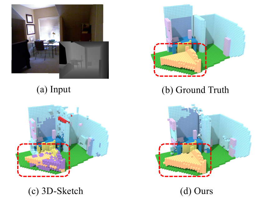
Figure 1: Visualization of Semantic Scene Completion task. Our method generates more reasonable results compared to 3D-Sketch (Chen et al. 2020a) while significantly lowering the computational costs.

With a partial 2D observation, humans are capable of understanding the 3D space and inferring the objects behind the occlusion. Similarly, the capability to capture the structure and semantic information of 3D scenes is beneficial for many real-world applications, including robotics, virtual reality, and interior design. To achieve this goal, we need to perform scene completion and scene labeling tasks, which are proved to be closely correlated by (Song et al. 2017). Semantic Scene Completion (SSC) is therefore put forward to predict 3D geometry and semantics simultaneously from a partial observation, which is an emerging topic in recent years.

Previously, most methods (Song et al. 2017; Guo and Tong 2018; Garbade et al. 2019; Liu et al. 2018) solve this challenging problem with voxelized partial observations. To handle these voxelized scenes, 3D convolution networks are always adopted by these methods to learn the occupancy and semantic information of each voxel. Although voxel representations preserve abundant structure details of the partial 2D observation, not all voxels are of equal importance in this volume. In particular, there exist lots of visible empty voxels (e.g., atmosphere in the visible region) in the voxelized SSC data by nature. These voxel-based methods have to perform unnecessary calculations on them in forward propagation, but ignore them in backward propagation since the labels are already known. Therefore, they always suffer from heavy computation redundancy, especially for trying to keep the high scene resolution in a deep 3D convolution network. To solve this problem, an efficient sparse data structure should be used, such as the point cloud or voxel octree (Liu et al. 2020; Takikawa et al. 2021). An early attempt (Zhong and Zeng 2020) removes these visible empty voxels and adopts a point cloud based network to extract features from this non-grid data for SSC task, but it is intrinsically weak in local structure modeling since the point cloud representation is sparse.

Therefore, it is crucial to consider the complementarity between voxel-based and point-based scene representation into the SSC framework. Unlike most other 3D computer vision tasks, such as 3D detection or segmentation, the data for SSC tasks is usually voxelized since the goal is to predict the semantic and occupancy of voxels in this 3D scene. The point clouds are extracted from these voxels. In fact, the voxel representation is denser than the point representation in our setting, for that only a part of point clouds are sampled as input during training. Thus, we design our Point-Voxel Aggregation Network (PVA-Net), where two 3D convolution layers keep the details from the voxelized scenes and a deep point cloud based network captures semantic information efficiently.

We adopt the point stream as the main stream of our network for its low memory requirement. Meanwhile, a light-weight voxel stream is used to extract structure details, which acts as a complement to the point stream. To efficiently fuse the point stream and the voxel stream, we propose a novel Anisotropic Voxel Aggregation (AVA) module to aggregate information in voxels for each center point. Given the position of a center point, we apply three ellipsoidal receptive fields to extract feature patterns from the voxels in different directions and concatenate them with the center point’s features. Moreover, we design a semantic-guided decoder that consists of several Semantic-aware Propagation (SP) modules, which encourages feature propagation between points belonging to the same semantic class.

We summarize our contributions as follows:

• To avoid the redundant computation in visible empty voxels in the SSC task, we convert the valid volume data to points and introduce the Point-Voxel Aggregation Network, which combines the low memory requirement of point-based methods and the local structure modelling ability of voxel-based methods.

• We propose the Anisotropic Voxel Aggregation module to efficiently fuse the structure information from a light-weight voxel stream into the point stream, and the Semantic-aware Propagation module to encourage feature propagation between points of the same semantic class.

• Our method outperforms state-of-the-arts by a large margin on two public benchmarks, with only depth images as the input.

2 Related Work

2.1 Deep Learning for 3D Scene Analysis

Learning semantic information of given scene with 3D information has drawn increasing attention in recent years. Rather than directly using 3D data, previous methods always focus on RGBD images (Xing et al. 2019a, b; Xing, Wang, and Zeng 2020; Chen et al. 2020b) to understand the semantic information of the given scene. Different from 2D images, 3D data have various data representations such as voxels and point clouds and can facilitate various different applications (Wang et al. 2021; Rong, Shiratori, and Joo 2021; Rong et al. 2021; Tang et al. 2022, 2023a, 2023b). Lots of methods have been proposed to handle different representations. 3D CNNs are the straightforward extension of 2D CNNs to 3D voxels. Early researches (Chang et al. 2015; Wu et al. 2015; Maturana and Scherer 2015; Zhou and Tuzel 2018) rely on 3D convolutions to process 3D voxel data in regular grids.

Point-based methods learn 3D point cloud representations directly by defining permutation-invariant point convolutions in irregular space. PointNet (Qi et al. 2017a) first uses a shared MLP on every point individually followed by global max-pooling to extract global features. Pointnet++ (Qi et al. 2017b) introduces hierarchical architectures to learn local features and increases modal capacity. Later works (Rethage et al. 2018; Landrieu and Simonovsky 2018; Wu et al. 2018; Zhao et al. 2019; Milioto et al. 2019; Komarichev, Zhong, and Hua 2019; Lang et al. 2019; Hu et al. 2020; Xu et al. 2021) focus on more effective and general point operations, such as explicit point convolution kernels where the weights can be directly learned without intermediate MLP representations (Hua, Tran, and Yeung 2018; Li et al. 2018; Thomas et al. 2019; Lin et al. 2020) and graph convolutions (Wu, Qi, and Li 2019; Li et al. 2019a; Wang et al. 2019a).

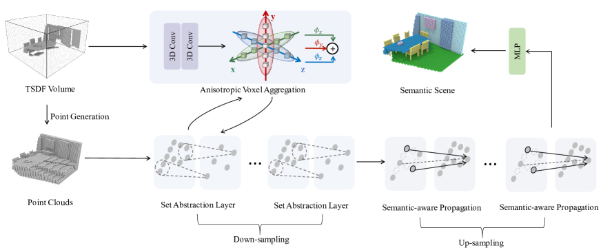
Figure 2: The overall architecture of the proposed method. We generate point clouds from input TSDF volumes and use an encoder-decoder architecture to predict the semantic labels, with an Anisotropic Voxel Aggregation module to aggregate the local structure information from the voxels.

Multi-modality fusion is also a long-term problem in 3D deep learning. Recently, a few works begin to leverage the advantages of point cloud and voxel representation together in deep neural networks. PV-CNN (Liu et al. 2019) is proposed to represent 3D data in sparse points to save memory cost and perform convolutions in voxels to obtain the contiguous memory access pattern. PV-RCNN (Shi et al. 2020) defines a Voxel Set Abstraction (VSA) module to summarize voxel features into key points to further explore this problem. However, this work focuses on object detection and relies on a heavy voxel stream to regress object proposals. To improve the learning efficiency and capability of the framework, we differ from the design choices in PV-RCNN as follows: 1) We only use a light-weight voxel stream to assist the main point stream; 2) Our AVA module is more general than the VSA module, which can be seen as a special case of our AVA module using spherical receptive fields; 3) We focus on scene completion and propose the SP module to aggregate features at different stages with semantic guidance during up-sampling, which is not considered by PV-RCNN.

2.2 Semantic Scene Completion

Semantic Scene Completion (SSC) aims to predict a complete voxel representation of a 3D scene and each voxel’s semantic label, usually from a single-view depth map observation. SSCNet (Song et al. 2017) first combines semantic segmentation and scene completion in an end-to-end way, showing that the two tasks are highly coupled and can be learned together to improve the performance. ESSCNet (Zhang et al. 2018) introduces Spatial Group Convolution (SGC) which divides the voxels into different groups to save computational cost. Later works (Guo and Tong 2018; Wang et al. 2019b; Zhang et al. 2019; Chen, Xing, and Zeng 2020) improve the performance with better architecture, such as 2D-3D combination, cascaded context pyramid and so on. Guedes et. al. (Guedes, Campos, and Hilton 2018) first investigates the potential of the RGB images to improve SSCNet. After that, many methods (Garbade et al. 2019; Liu et al. 2018; Dourado et al. 2019; Li et al. 2019b, 2020b; Chen et al. 2020a) take RGB images as an additional input with the depth map and explore the complementarity between the two modalities. Most recent work (Li, Ding, and Huang 2021) further explores the interaction between 2D segmentation and 3D SSC, but they rely on heavy networks to perform the feature extraction.

These methods all utilize 3D CNNs as the backbone, causing unnecessary computational cost in the visible empty voxels. Whereas AIC-Net (Li et al. 2020a) also proposes an anisotropic convolution to model the voxel-wisely dimensional anisotropy, our AVA module differs in both formulation and functionality, focusing on synchronizing features from voxels to point representation with a more flexible ellipsoidal receptive field.

Different from those voxel-based methods above, SPCNet (Zhong and Zeng 2020) first introduces a point-based network to address the SSC problem, by training a point network on the observed points and then obtaining the features of the occluded points through bilinear interpolation. Due to the interpolation process that depends on distance metrics, the occluded points far from the visible points are hard to predict in their method. Furthermore, point-based method alone is not enough to retain detailed local structure information during the down-sampling progress. Therefore, we draw ideas from the Point-Voxel methods and propose a two-stream network, where an efficient point stream extracts semantic features and a light-weight voxel stream provides dense local structure information through the AVA module.

3 Methodology

3.1 Overview of the Proposed Method

The overall architecture of the proposed method is illustrated in Figure 2. Our model consists of a point stream and a voxel stream. To reduce the computation redundancy, we convert the TSDF volume to a point cloud by removing the visible empty voxels, which serves as the input of the point stream. The point stream adopts a PointNet++ (Qi et al. 2017b)-like encoder-decoder architecture. The encoder extracts the semantic features in a hierarchical way and the decoder encourages feature propagation in points of the same class. Meanwhile, a light-weight voxel stream that only contains two 3D dense convolutional layers is applied to the TSDF volume. An AVA module is proposed to aggregate the local voxel features to the point features. Finally, the predicted point labels are converted back to the voxel representation to calculate the evaluation metrics.

3.2 Point Clouds Generation

Voxel-based methods always encode the depth map into a 3D TSDF volume (Song et al. 2017), and carry out later procedures in this voxel space. However, we argue that not all voxels in this volume are of equal importance for the SSC task. In fact, there are three kinds of voxels inside this volume: 1) the observed surface voxels which are directly projected from the given depth image, 2) the occluded voxels behind the observed surface which we need to complete and recognize, and 3) the visible empty voxels (such as the atmosphere) between camera and the observed surface. The last kind of voxel is useless for our task since we already know it’s empty. Thus, these voxels are removed during our point clouds generation process. As shown in Figure 3, we only keep the observed surface and the occluded regions in our point clouds.

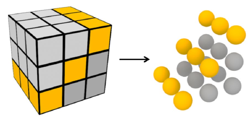
Figure 3: Points generation from the voxel volumes. Only the observed surface (yellow) and occluded regions (dark gray) are kept, while the visible empty voxels (light gray) are discarded. For example, the average number of the kept points is 16313 for the 60 $\times$ 36 $\times$ 60 input voxels from the NYUCAD dataset, which means about 87% of the input voxels are redundant.

Each input point $\mathbf{p}_{i}$ has a $5$-dim feature vector $\mathbf{f}_{i}=(x_{i},y_{i},z_{i},t_{i},h_{i})$. Suppose $\mathbf{p}_{i}$ is generated from voxel $\mathbf{v}_{i}$ in the $60\times 36\times 60$ 3D volume, then $x_{i},y_{i},z_{i}$ are normalized $x$-$y$-$z$ indexes of $\mathbf{v}_{i}$ in the volume. $t_{i}$ is the TSDF value of $\mathbf{v}_{i}$, and $h_{i}$ is the normalized height value of $\mathbf{v}_{i}$. Please note that $x_{i},y_{i},z_{i}$ are normalized according to the mass center of the points in the scene, while $h_{i}$ is normalized by $36$, the maximum height of the voxelized scene. We think the normalized height serves as a prior that describes the positions of objects in the room. This could help to distinguish some categories with significantly different height values, such as the floor and the ceiling.

3.3 Anisotropic Voxel Aggregation

Due to the sparsity of the point clouds, it is hard for the point stream to model the detailed structure information which is important for the scene completion and recognition. Since we have the denser volume data as well, we design a voxel stream to extract the structure features and propose the Anisotropic Voxel Aggregation (AVA) module to fuse the point-voxel features.

We first extract the local features of the TSDF volume through two simple convolution layers. This requires little computational cost and takes about only 15.0% of the overall memory cost, but enables each voxel in the volume to have a suitable receptive field to encode local geometry information. As shown in the top part of Figure 2, for each center point $\mathbf{p}_{i}=(x_{i},y_{i},z_{i})$ in the point cloud, we define three ellipsoidal receptive fields with $x,y,z$ axis as the major axis respectively. Taking the $x$-axis as an example, the receptive field $\mathcal{N}_{x}(i)$ of $\mathbf{p}_{i}$ in the volume could be defined as:

where $\mathbf{v}_{j}$ is the $j$-th voxel and $(x_{j},y_{j},z_{j})$ is its position, $r$ is the radius for minor axes, and $k>1$ is a scale factor for the major axis. Unless mentioned specifically, we use $3$ as the default value for $k$. The receptive field along the $y$-axis and $z$-axis could be defined in a similar way. From the perspective of pattern recognition, the anisotropic receptive field ensures us to activate feature patterns in three directions, which is more flexible and effective than the isotropic spherical receptive field.

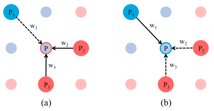
Figure 4: Different Feature Propagation strategies. (a) Feature Propagation (FP) in PointNet++ (Qi et al. 2017b). (b) The proposed Semantic-aware Propagation (SP). Different colors mean different semantic classes. Larger points are from a deeper layer, while smaller points are in the current layer. Dashed lines mean smaller weight. The boundary color of the center point means the interpolated features are dominated by which semantic class. In (a), the center point is dominated by the wrong class due to the unsuitable FP strategy, while the proposed method (b) avoids this problem.

Then we could aggregate the structure features of voxels around $\mathbf{p}_{i}$ with:

$$\mathbf{f}^{\text{fuse}}_{i}=\sum_{d\in\{x,y,z\}}\max_{j\in\mathcal{N}_{d}(i)}\{\phi_{d}(\mathbf{f}^{\text{point}}_{i},\mathbf{f}^{\text{voxel}}_{j})\}$$ (2)

where $\mathbf{f}^{\text{fuse}}_{i}$ is the fused point-voxel feature, $\mathbf{f}^{\text{point}}_{i}$ is the feature of $\mathbf{p}_{i}$, $\mathbf{f}^{\text{voxel}}_{j}$ is the feature of $j$-th voxel in the volume, $\phi_{d}$ is a MLP layer for non-linear feature extraction in the $d$-axis, $\max$ denotes max-pooling operation that keeps the maximum activation in the neighborhood, and $\mathcal{N}_{d}(i)$ represents the set of neighbor voxels of $\mathbf{p}_{i}$ inside the ellipsoidal receptive field with the $d$-axis as the major axis. This AVA module enables the sparse center points to aggregate local structure information from nearby dense voxels. Therefore, the information from voxels could positively affect the completion and recognition of point clouds through back propagation.

3.4 Semantic-aware Propagation

During the encoding process, Set Abstract (SA) (Qi et al. 2017b) layers will down-sample the input points. Suppose we have $N$ SA layers in the network, named $\text{SA}^{(1)}$, …, $\text{SA}^{(N)}$. We denote $\mathbf{X}^{(0)}=\{(\mathbf{p}^{(0)}_{i},\mathbf{f}^{(0)}_{i})\}$ as the raw input point set, where $\mathbf{f}^{(0)}_{i}$ is the feature of the point $\mathbf{p}^{(0)}_{i}$. Then the corresponding output point sets of $N$ SA layers are $\mathbf{X}^{(1)}$, …, $\mathbf{X}^{(N)}$, respectively. Please note that if a point belongs to $\mathbf{X}^{(i)}$ ($i\geq 1$), then it must belong to $\mathbf{X}^{(i-1)}$ as well, because each SA layer only down-samples points from the former layer.

To obtain the features of all the raw input points, we propose the Semantic-aware Propagation (SP) module, which is a hierarchical propagation strategy as shown in Figure 4. For a target point $\mathbf{p}^{(l)}_{i}$ in $\mathbf{X}^{(l)}$, we find its $k$-neighbors ($\mathbf{p}^{(l+1)}_{1}$, …, $\mathbf{p}^{(l+1)}_{k}$) in $\mathbf{X}^{(l+1)}$ according to the $xyz$ coordinates. To interpolate the feature of $\mathbf{p}^{(l)}$, the general feature propagation can be represented by:

$$\mathbf{f}^{(l)}_{i}=\frac{\sum_{j\in\mathcal{N}_{k}^{(l+1)}(i)}w_{i,j}^{(l)}\mathbf{f}_{j}^{(l+1)}}{\sum_{j\in\mathcal{N}_{k}^{(l+1)}(i)}w_{i,j}^{(l)}}$$ (3)

where $\mathcal{N}_{k}^{(l+1)}(i)$ is the set of $k$ nearest neighbors of $\mathbf{p}^{(l)}_{i}$ in $\mathbf{X}^{(l+1)}$, and $w_{i,j}^{(l)}$ is the weight factor for $\mathbf{f}^{(l+1)}_{j}$ with respect to the point $\mathbf{p}^{(l)}_{i}$.

An intuitive idea is to measure the similarity between the point $\mathbf{p}_{i}^{(l)}$ and $\mathbf{p}^{(l+1)}_{j}$ for $j\in\mathcal{N}_{k}^{(l+1)}(i)$ and use the similarity as the weight factor. However, since $\mathbf{p}_{i}^{(l)}$ and $\mathbf{p}^{(l+1)}_{j}$ belong to different levels and thus are embedded to different feature spaces, it is not suitable to directly compare their feature vectors. We notice that the point $\mathbf{p}^{(l+1)}_{j}$ also exists in $\mathbf{X}^{(l)}$ since the points in $\mathbf{X}^{(l+1)}$ is a subset of $\mathbf{X}^{(l)}$. Then we could measure the similarity between $\mathbf{p}_{i}^{(l)}$ and $\mathbf{p}^{(l)}_{j}$ in a learnable manner:

$$w_{i,j}^{(l)}=\sigma(\phi(\mathbf{f}_{i}^{(l)}||\mathbf{f}_{j}^{(l)}))$$ (4)

where $\sigma$ is the sigmoid function, $\phi$ is a MLP and $||$ means channel-wise concatenation.

In this way, we could interpolate point features with semantic information, which is helpful in SSC task. We explicitly supervise the learned weights during training, by setting the ground truth of $w_{i,j}^{(l)}$ to $1$ if the two points belong to the same semantic class, and $0$ if they belong to different classes. We think this could encourage the network to only propagate semantically similar features, which weakens the effect of neighbor points from different classes during interpolation.

3.5 Training Loss

The training loss involves two terms: SSC loss $\mathcal{L}_{\text{SSC}}$ and SP loss $\mathcal{L}_{\text{SP}}$. The SSC loss is a weighted voxel-wise cross-entropy loss:

$$\mathcal{L}_{\text{SSC}}=\frac{1}{N_{\text{valid}}}\sum_{i,j,k}m_{i,j,k}\mathcal{L}_{\text{CE}}(p_{i,j,k},\,y_{i,j,k})$$ (5)

where $m_{i,j,k}$ is set to $1$ if the voxel at index $(i,j,k)$ is not visible empty (i.e., can be converted to a point) or $0$ otherwise. $y_{i,j,k}$ is the ground truth label, $p_{i,j,k}$ is the prediction of the voxel mapped back from the corresponding point, $N_{\text{valid}}=\sum_{i,j,k}m_{i,j,k}$ is the number of valid voxels in this volume, and $\mathcal{L}_{\text{CE}}$ is the cross-entropy loss.

The SP loss is designed to supervise the pairwise similarity introduced in Equation 4. The SP loss could be formulated as:

$$\mathcal{L}_{\text{SP}}=\frac{1}{N_{\text{pairs}}}\sum_{l}\sum_{0\leq i\leq\lvert\mathbf{X}^{(l)}\rvert}\sum_{j\in\mathcal{N}_{k}^{(l+1)}(i)}\mathcal{L}_{\text{CE}}(w_{i,j}^{(l)},\,\mathbf{G}_{i,j}^{(l)})$$ (6)

where $N_{\text{pairs}}$ represents the number of point pairs involved, $\smash{\lvert}\mathbf{X}^{(l)}\rvert$ means the number of points in the $l$-th level, ${\mathcal{N}_{k}^{(l+1)}(i)}$ is defined in Section 3.4. ${\mathbf{G}_{i,j}^{(l)}}$ is the ground truth of the pair-wise similarity. If two points $\mathbf{p}_{i}^{(l)}$ and $\mathbf{p}_{j}^{(l)}$ belong to the same category, it is 1, otherwise it is 0.

We optimize the entire network by the balanced combination of the two terms:

$$\mathcal{L}=\mathcal{L}_{\text{SSC}}+\lambda\mathcal{L}_{\text{SP}}$$ (7)

4 Experiments

In this section, we evaluate the proposed method and compare it with state-of-the-art methods on two public datasets, NYU (Silberman et al. 2012) and NYUCAD (Firman et al. 2016).

4.1 Datasets and Evaluation Metrics

Datasets.

The NYU dataset (Silberman et al. 2012) consists of $1,449$ realistic indoor RGB-D scenes captured via a Kinect sensor (Song et al. 2017). Since the real-world completed scenes are hard to be captured, human annotations provided by (Guo, Zou, and Hoiem 2015) are widely used as the ground truth completion. However, as discussed in (Song et al. 2017), there exists many misalignments between the depth images and the corresponding 3D labels in the NYU dataset, which makes it hard to evaluate accurately. To solve this problem, the high-quality synthetic NYUCAD dataset is proposed by (Firman et al. 2016), where the depth maps are projected from the ground truth annotations and thus avoid the misalignments. Following previous works (Song et al. 2017; Chen et al. 2020a; Garbade et al. 2019), we choose NYU and NYUCAD to evaluate our method.

Evaluation Metrics.

We follow (Song et al. 2017) to use precision, recall and voxel-level intersection over union (IoU) as the evaluation metrics. Two tasks are considered, namely, semantic scene completion and scene completion. For the task of semantic scene completion, we evaluate on both the observed surface and occluded regions and report the mIoU of each semantic class. For the task of scene completion, we treat all non-empty voxels as class ‘1’ and all empty voxels as class ‘0’, and then evaluate the binary IoU on the occluded regions.

			scene completion			semantic scene completion
Methods	Input	Resolution	prec.	recall	IoU	ceil.	floor	wall	win.	chair	bed	sofa	table	tvs	furn.	objs.	mIoU
Zheng $et\,al.$ (Zheng et al. 2013)	D	(240, 60)	60.1	46.7	34.6	-	-	-	-	-	-	-	-	-	-	-	-
Firman $et\,al.$ (Firman et al. 2016)	D	(240, 60)	66.5	69.7	50.8	-	-	-	-	-	-	-	-	-	-	-	-
SSCNet (Song et al. 2017)	D	(240, 60)	75.4	96.3	73.2	32.5	92.6	40.2	8.9	33.9	57.0	59.5	28.3	8.1	44.8	25.1	40.0
CCPNet (Zhang et al. 2019)	D	(240, 240)	91.3	92.6	82.4	56.2	94.6	58.7	35.1	44.8	68.6	65.3	37.6	35.5	53.1	35.2	53.2
SPCNet (Zhong and Zeng 2020)	D	(60, 60)	81.4	70.9	61.0	58.1	91.6	53.7	13.0	52.1	68.9	57.7	31.9	6.4	50.5	28.1	46.6
TS3D (Garbade et al. 2019)	RGB+D	(240, 60)	-	-	76.1	25.9	93.8	48.9	33.4	31.2	66.1	56.4	31.6	38.5	51.4	30.8	46.2
DDRNet (Li et al. 2019b)	RGB+D	(240, 60)	88.7	88.5	79.4	54.1	91.5	56.4	14.9	37.0	55.7	51.0	28.8	9.2	44.1	27.8	42.8
AIC-Net (Li et al. 2020a)	RGB+D	(240, 60)	88.2	90.3	80.5	53.0	91.2	57.2	20.2	44.6	58.4	56.2	36.2	9.7	47.1	30.4	45.8
3D-Sketch (Chen et al. 2020a)	RGB+D	(60, 60)	90.6	92.2	84.2	59.7	94.3	64.3	32.6	51.7	72.0	68.7	45.9	19.0	60.5	38.5	55.2
IMENet (Li, Ding, and Huang 2021)	RGB+D	(60, 60)	84.8	92.3	79.1	-	-	-	-	-	-	-	-	-	-	-	47.5
Ours	D	(60, 60)	95.1	90.3	86.3	71.5	94.1	66.6	23.7	60.0	78.5	72.2	45.3	16.7	60.1	36.9	56.9

Table 1: Results on the NYUCAD dataset. Resolution(a, b) means the input resolution is $(a\times 0.6a\times a)$ and the output resolution is $(b\times 0.6b\times b)$.

			scene completion			semantic scene completion
Methods	Input	Resolution	prec.	recall	IoU	ceil.	floor	wall	win.	chair	bed	sofa	table	tvs	furn.	objs.	mIoU
SSCNet (Song et al. 2017)	D	(240,60)	57.0	94.5	55.1	15.1	94.7	24.4	0.0	12.6	32.1	35.0	13.0	7.8	27.1	10.1	24.7
ESSCNet (Zhang et al. 2018)	D	(240,60)	71.9	71.9	56.2	17.5	75.4	25.8	6.7	15.3	53.8	42.4	11.2	0	33.4	11.8	26.7
VVNet (Guo and Tong 2018)	D	(120,60)	69.8	83.1	61.1	19.3	94.8	28.0	12.2	19.6	57.0	50.5	17.6	11.9	35.6	15.3	32.9
ForkNet (Wang et al. 2019b)	D	(80,80)	-	-	63.4	36.2	93.8	29.2	18.9	17.7	61.6	52.9	23.3	19.5	45.4	20.0	37.1
CCPNet (Zhang et al. 2019)	D	(240,240)	74.2	90.8	63.5	23.5	96.3	35.7	20.2	25.8	61.4	56.1	18.1	28.1	37.8	20.1	38.5
SPCNet (Zhong and Zeng 2020)	D	(240,60)	72.1	42.2	36.3	33.8	64.4	38.3	7.5	30.7	53.4	42.6	19.7	5.5	34.2	13.9	31.3
TS3D (Garbade et al. 2019)	RGB+D	(240,60)	-	-	60.0	9.7	93.4	25.5	21.0	17.4	55.9	49.2	17.0	27.5	39.4	19.3	34.1
SATNet (Liu et al. 2018)	RGB+D	(60,60)	67.3	85.8	60.6	17.3	92.1	28.0	16.6	19.3	57.5	53.8	17.2	18.5	38.4	18.9	34.4
DDRNet (Li et al. 2019b)	RGB+D	(60,60)	71.5	80.8	61.0	21.1	92.2	33.5	6.8	14.8	48.3	42.3	13.2	13.9	35.3	13.2	30.4
AIC-Net (Li et al. 2020a)	RGB+D	(60,60)	62.4	91.8	59.2	23.2	90.8	32.3	14.8	18.2	51.1	44.8	15.2	22.4	38.3	15.7	33.3
3D-Sketch (Chen et al. 2020a)	RGB+D	(60,60)	85.0	81.6	71.3	43.1	93.6	40.5	24.3	30.0	57.1	49.3	29.2	14.3	42.5	28.6	41.1
IMENet (Li, Ding, and Huang 2021)	RGB+D	(60,60)	90.0	78.4	72.1	43.6	93.6	42.9	31.3	36.6	57.6	48.4	32.1	16.0	47.8	36.7	44.2
Ours	D	(60,60)	91.1	79.7	74.0	51.4	94.0	49.9	15.9	41.9	68.3	58.8	35.4	12.9	48.5	29.1	46.0

Table 2: Results on the NYU dataset. Resolution(a, b) means the input resolution is $(a\times 0.6a\times a)$ and the output resolution is $(b\times 0.6b\times b)$.

4.2 Implementation Details

We use the PyTorch framework with two Nvidia Titan Xp GPUs to conduct our experiments. Mini-batch SGD with momentum of $0.9$ is adopted to train our network. The initial learning rate is $0.05$, batch size is $8$ and the weight decay is $0.0005$. We employ a Poly learning rate decay policy where the initial learning rate is multiplied by $(1-\frac{\text{now\_iter}}{\text{max\_iter}})^{0.9}$. We train our network for $1000$ epochs on the NYUCAD dataset and the NYU dataset. The radius of the ellipsoidal receptive field is set to $0.09$ for the major axis and $0.03$ for the minor axes. We sample at most $8$ voxels inside each ellipsoidal receptive field. The balancing factor $\lambda$ in Equation 7 is set to $0.5$. Since the output of the SSC task is usually at the resolution of 60 $\times$ 36 $\times$ 60, we adopt the same input resolution of voxels following SATNet (Liu et al. 2018) and 3D-Sketch (Chen et al. 2020a). Different from (Zhong and Zeng 2020), we feed both the observed and occluded points into our network during training. Since the number of points for each scene is not fixed, we randomly sample a fixed number of observed points ($2048$) and occluded points ($8192$) for each scene to enable batched training. At inference time, we use all the generated points as input.

4.3 Comparisons with State-of-the-art Methods

We compare the proposed method with state-of-the-art methods. Table 1 lists the results on the NYUCAD dataset. Our method outperforms all the existing voxel-based or point-based methods, gaining an increase of $1.7\%$ SSC mIoU and $2.1\%$ SC IoU compared to the previous best method (Chen et al. 2020a). While some methods use a higher input resolution, we already achieve good enough results with the 60 $\times$ 36 $\times$ 60 input resolution. The advantage of our method is not from a higher input resolution than others, but the novel and efficient point-voxel framework that modelling the local details and global context in a computationally-friendly manner. We also conduct experiments on the NYU dataset to validate the performance of our method on realistic data. As listed in Table 2, our method consistently outperforms previous best method (Li, Ding, and Huang 2021) in both SC IoU and SSC mIoU metrics. Notably, our method only requires one-pass forward, while IMENet (Li, Ding, and Huang 2021) performs multiple iterations between a 2D and a 3D network and introduces a very large computational cost.

We provide some visualizations on the NYUCAD dataset in Figure 5. With only the depth images as input, our method achieves good inter-class distinction and intra-class consistency. We think the superiority of the proposed method comes from the two-stream framework, where the point stream extracts the high-level semantics and the voxel stream extracts the detailed local structure information.

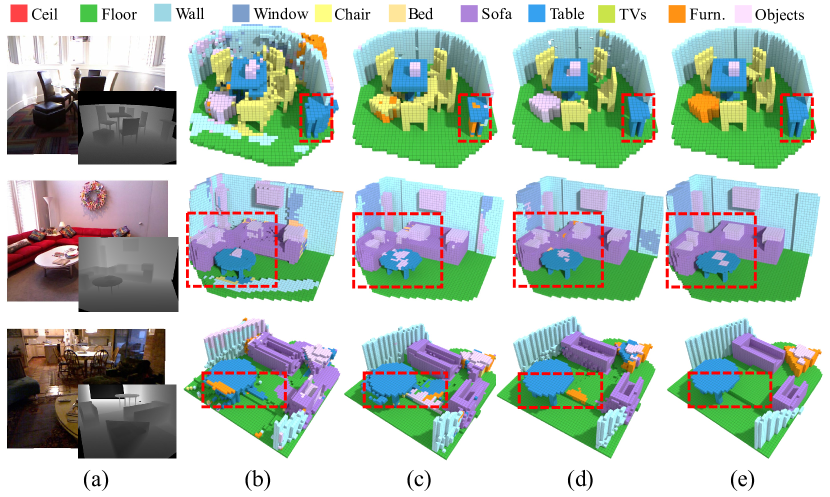
Figure 5: Visualizations on the NYUCAD dataset. From left to right: (a) RGB-D images, (b) results of (Song et al. 2017), (c) results of (Chen et al. 2020a), (d) our results, and (e) ground truth. Best viewed in color and zoom in.

Methods	FLOPs	Memory	SC IoU(%)	SSC mIoU(%)
SSCNet	163.8G	1057M	73.2	40.0
3D-Sketch	293.7G	1535M	84.2	55.2
Ours	8.9G	554M	86.3	56.9

Table 3: Efficiency analysis on the NYUCAD dataset.

4.4 Efficiency Analysis

Since the computational cost of our method depends on the number of visible empty points in each scene, we report the average number of these statistics on the NYUCAD test set in Table 3. The proposed method avoids the redundancy caused by the visible empty voxels and achieves higher performance with lower computational cost. Even though our FLOPs are only $5.4\%$ of SSCNet and $3.0\%$ of 3D-Sketch, we still achieve a better performance.

4.5 Ablation Study

In this section, we conduct ablation studies to verify the effectiveness of each aforementioned component. All the results are tested on the NYUCAD test set.

Proposed modules.

Firstly, we do ablation studies on different modules in our method in Table 4. The AVA module aggregates the local structure information from the voxel stream to the point stream, and the SP module encourages feature propagation of points belonging to the same category. Adopting either of these two modules improves the performance, and the combination of them achieves the maximum benefits. Note that our point-based baseline already outperforms some of the voxel-based methods. Thanks to the removal of redundant parts in the input, the point stream could have a deeper architecture and higher feature dimensions, leading to stronger representation power.

Baseline	AVA	SP	SC IoU(%)	SSC mIoU(%)
✓			85.1	51.4
✓		✓	85.9	53.2
✓	✓		85.3	54.9
✓	✓	✓	86.3	56.9

Table 4: Ablation study on different modules. The baseline is a pure point-based network (PointNet++(Qi et al. 2017b)), ‘AVA’ means Anisotropic Voxel Aggregation and ‘SP’ means Semantic-aware Propagation.

Methods	SC IoU(%)	SSC mIoU(%)
Point Only	85.9	53.2
Nearest Aggregation	86.0	55.1
Spherical Aggregation	86.1	56.0
Anisotropic Voxel Aggregation	86.3	56.9

Table 5: Ablation study on different Voxel Aggregation Strategies.

Voxel Aggregation Strategies.

As illustrated before, we propose the AVA module that aggregates the voxel structure features in an anisotropic manner. Here, we try to compare AVA with other voxel aggregation strategies to verify its effectiveness. We provide two other strategies: ‘Nearest Aggregation’ and ‘Spherical Aggregation’. ‘Nearest Aggregation’ means we only concatenate the point features with the features of the nearest voxel from the point. ‘Spherical Aggregation’ means we adopt a spherical receptive field with the radius $r$ to aggregate the voxel features inside the receptive field. $r$ is $0.09$ here so that it is the same with the radius of the major axis in AVA. Results are listed in Table 5. As shown in the table, both ‘Nearest Aggregation’ and ‘Spherical Aggregation’ could boost the performance, because they more or less introduce some detailed geometric information to the point stream. However, the proposed AVA module achieves the best performance with the anisotropic aggregation design, because it could capture more feature patterns in different directions.

Position of the AVA Module.

We try to embed AVA modules to different positions in the network, as listed in Table 6. We find that if we embed the AVA module to a higher level layer in the network, the additional gain brought by voxel features decreases. This makes sense for that the AVA module exploits local features in the voxel representation and if we embed it into the first SA layer, the structure information provided by the AVA module will be further encoded as the network goes deeper. Also, if we embed AVA modules to all the SA layers in the network, the performance is just similar to the proposed method. Hence, we only embed it to the first SA layer for lower computational cost.

Feature Propagation Strategies.

We then conduct experiments on the proposed SP module. The SP module encourages feature propagation in points belonging to the same category through the $w_{i,j}$ defined in Equation 3 and Equation 4. We compare SP with other feature propagation strategies in Table 7. Our SP achieves the best performance, since it considers pairwise semantic relations and avoids the errors caused by feature propagation from the wrong categories.

SA-1	SA-2	SA-3	SA-4	SC IoU(%)	SSC mIoU(%)
✓				86.3	56.9
	✓			86.2	55.7
		✓		86.0	53.4
			✓	85.8	53.8
✓	✓	✓	✓	86.2	56.6

Table 6: Ablation study on the position of AVA module. SA-$i$ indicates AVA module is embedded into the $i$-th SA layer.

Methods	SC IoU(%)	SSC mIoU(%)
Inverse Euclidean	85.3	54.9
Cosine Similarity	83.9	54.4
Semantic-aware Propagation	86.3	56.9

Table 7: Ablation study on different Feature Propagation Strategies. ‘Inverse Euclidean’ means the inverse Euclidean distance between two points used in Pointnet++ (Qi et al. 2017b). ‘Cosine Similarity’ means the cosine similarity between features of the two points. The proposed SP module achieves the best performance.

5 Conclusion

In this paper, we introduce the Point-Voxel Aggregation Network for Semantic Scene Completion, which combines the advantages of the computationally efficient point representation and the rich-detailed voxel representation. Besides, an AVA module is proposed to aggregate the structure information from voxels and a SP module is proposed to encourage semantic-aware feature propagation in points. Experimental results demonstrate the effectiveness and efficiency of our method with state-of-the-art performance on two public benchmarks, with only the depth images as input. In the future, we believe the representation of the scene is crucial for this topic, such as the modality of inputs (e.g., RGB and depth map), as well as the point cloud with different sampling rates.

References

- Chang et al. (2015) Chang, A. X.; Funkhouser, T.; Guibas, L.; Hanrahan, P.; Huang, Q.; Li, Z.; Savarese, S.; Savva, M.; Song, S.; Su, H.; Xiao, J.; Yi, L.; and Yu, F. 2015. ShapeNet: An Information-Rich 3D Model Repository. ArXiv, abs/1512.03012.
- Chen et al. (2020a) Chen, X.; Lin, K.-Y.; Qian, C.; Zeng, G.; and Li, H. 2020a. 3D Sketch-aware Semantic Scene Completion via Semi-supervised Structure Prior. In CVPR, 4193–4202.
- Chen et al. (2020b) Chen, X.; Lin, K.-Y.; Wang, J.; Wu, W.; Qian, C.; Li, H.; and Zeng, G. 2020b. Bi-directional cross-modality feature propagation with separation-and-aggregation gate for RGB-D semantic segmentation. In ECCV, 561–577. Springer.
- Chen, Xing, and Zeng (2020) Chen, X.; Xing, Y.; and Zeng, G. 2020. Real-Time Semantic Scene Completion Via Feature Aggregation And Conditioned Prediction. In ICIP, 2830–2834. IEEE.
- Dourado et al. (2019) Dourado, A.; Campos, T. D.; Kim, H.; and Hilton, A. 2019. EdgeNet: Semantic Scene Completion from RGB-D images. ArXiv, abs/1908.02893.
- Firman et al. (2016) Firman, M.; Mac Aodha, O.; Julier, S.; and Brostow, G. J. 2016. Structured prediction of unobserved voxels from a single depth image. In CVPR, 5431–5440.
- Garbade et al. (2019) Garbade, M.; Sawatzky, J.; Richard, A.; and Gall, J. 2019. Two Stream 3D Semantic Scene Completion. In CVPR Workshop.
- Guedes, Campos, and Hilton (2018) Guedes, A. B. S.; Campos, T. D.; and Hilton, A. 2018. Semantic Scene Completion Combining Colour and Depth: preliminary experiments. In ArXiv, volume abs/1802.04735.
- Guo, Zou, and Hoiem (2015) Guo, R.; Zou, C.; and Hoiem, D. 2015. Predicting Complete 3D Models of Indoor Scenes. ArXiv, abs/1504.02437.
- Guo and Tong (2018) Guo, Y.-X.; and Tong, X. 2018. View-Volume Network for Semantic Scene Completion from a Single Depth Image. ArXiv, abs/1806.05361.
- Hu et al. (2020) Hu, Q.; Yang, B.; Xie, L.; Rosa, S.; Guo, Y.; Wang, Z.; Trigoni, A.; and Markham, A. 2020. RandLA-Net: Efficient Semantic Segmentation of Large-Scale Point Clouds. In CVPR, 11105–11114.
- Hua, Tran, and Yeung (2018) Hua, B.-S.; Tran, M.-K.; and Yeung, S.-K. 2018. Pointwise convolutional neural networks. In CVPR, 984–993.
- Komarichev, Zhong, and Hua (2019) Komarichev, A.; Zhong, Z.; and Hua, J. 2019. A-CNN: Annularly Convolutional Neural Networks on Point Clouds. In CVPR, 7413–7422.
- Landrieu and Simonovsky (2018) Landrieu, L.; and Simonovsky, M. 2018. Large-Scale Point Cloud Semantic Segmentation with Superpoint Graphs. In CVPR, 4558–4567.
- Lang et al. (2019) Lang, A. H.; Vora, S.; Caesar, H.; Zhou, L.; Yang, J.; and Beijbom, O. 2019. PointPillars: Fast Encoders for Object Detection From Point Clouds. In CVPR, 12689–12697.
- Li et al. (2019a) Li, G.; Müller, M.; Thabet, A. K.; and Ghanem, B. 2019a. DeepGCNs: Can GCNs Go As Deep As CNNs? In ICCV, 9266–9275.
- Li, Ding, and Huang (2021) Li, J.; Ding, L.; and Huang, R. 2021. IMENet: Joint 3D Semantic Scene Completion and 2D Semantic Segmentation through Iterative Mutual Enhancement. arXiv preprint arXiv:2106.15413.
- Li et al. (2020a) Li, J.; Han, K.; Wang, P.; Liu, Y.; and Yuan, X. 2020a. Anisotropic Convolutional Networks for 3D Semantic Scene Completion. In CVPR, 3351–3359.
- Li et al. (2019b) Li, J.; Liu, Y.; Gong, D.; Shi, Q.; Yuan, X.; Zhao, C.; and Reid, I. 2019b. RGBD Based Dimensional Decomposition Residual Network for 3D Semantic Scene Completion. In CVPR, 7685–7694.
- Li et al. (2020b) Li, S.; Zou, C.; Li, Y.; Zhao, X.; and Gao, Y. 2020b. Attention-based Multi-modal Fusion Network for Semantic Scene Completion. ArXiv.
- Li et al. (2018) Li, Y.; Bu, R.; Sun, M.; Wu, W.; Di, X.; and Chen, B. 2018. PointCNN: Convolution On X-Transformed Points. In NeurIPS.
- Lin et al. (2020) Lin, Y.; Yan, Z.; Huang, H.; Du, D.; Liu, L.; Cui, S.; and Han, X. 2020. FPConv: Learning Local Flattening for Point Convolution. In CVPR, 4293–4302.
- Liu et al. (2020) Liu, L.; Gu, J.; Lin, K. Z.; Chua, T.-S.; and Theobalt, C. 2020. Neural sparse voxel fields. arXiv preprint arXiv:2007.11571.
- Liu et al. (2018) Liu, S.; Hu, Y.; Zeng, Y.; Tang, Q.; Jin, B.; Han, Y.; and Li, X. 2018. See and Think: Disentangling Semantic Scene Completion. In NeurIPS, 261–272.
- Liu et al. (2019) Liu, Z.; Tang, H.; Lin, Y.; and Han, S. 2019. Point-voxel cnn for efficient 3d deep learning. In NeurIPS, volume 32, 965–975.
- Maturana and Scherer (2015) Maturana, D.; and Scherer, S. 2015. Voxnet: A 3d convolutional neural network for real-time object recognition. In IROS, 922–928. IEEE.
- Milioto et al. (2019) Milioto, A.; Vizzo, I.; Behley, J.; and Stachniss, C. 2019. RangeNet ++: Fast and Accurate LiDAR Semantic Segmentation. In IROS, 4213–4220.
- Qi et al. (2017a) Qi, C. R.; Su, H.; Mo, K.; and Guibas, L. J. 2017a. Pointnet: Deep learning on point sets for 3d classification and segmentation. In CVPR, 652–660.
- Qi et al. (2017b) Qi, C. R.; Yi, L.; Su, H.; and Guibas, L. J. 2017b. Pointnet++: Deep hierarchical feature learning on point sets in a metric space. In NeurIPS, volume 30, 5099–5108.
- Rethage et al. (2018) Rethage, D.; Wald, J.; Sturm, J.; Navab, N.; and Tombari, F. 2018. Fully-Convolutional Point Networks for Large-Scale Point Clouds. In ArXiv, volume abs/1808.06840.
- Rong, Shiratori, and Joo (2021) Rong, Y.; Shiratori, T.; and Joo, H. 2021. Frankmocap: A monocular 3d whole-body pose estimation system via regression and integration. In ICCV, 1749–1759.
- Rong et al. (2021) Rong, Y.; Wang, J.; Liu, Z.; and Loy, C. C. 2021. Monocular 3D Reconstruction of Interacting Hands via Collision-Aware Factorized Refinements. arXiv preprint arXiv:2111.00763.
- Shi et al. (2020) Shi, S.; Guo, C.; Jiang, L.; Wang, Z.; Shi, J.; Wang, X.; and Li, H. 2020. PV-RCNN: Point-Voxel Feature Set Abstraction for 3D Object Detection. In CVPR, 10526–10535.
- Silberman et al. (2012) Silberman, N.; Hoiem, D.; Kohli, P.; and Fergus, R. 2012. Indoor Segmentation and Support Inference from RGBD Images. In ECCV.
- Song et al. (2017) Song, S.; Yu, F.; Zeng, A.; Chang, A. X.; Savva, M.; and Funkhouser, T. 2017. Semantic scene completion from a single depth image. In CVPR, 1746–1754.
- Takikawa et al. (2021) Takikawa, T.; Litalien, J.; Yin, K.; Kreis, K.; Loop, C.; Nowrouzezahrai, D.; Jacobson, A.; McGuire, M.; and Fidler, S. 2021. Neural geometric level of detail: Real-time rendering with implicit 3D shapes. In CVPR, 11358–11367.
- Tang et al. (2022) Tang, J.; Chen, X.; Wang, J.; and Zeng, G. 2022. Compressible-composable NeRF via Rank-residual Decomposition.
- Tang et al. (2023a) Tang, J.; Chen, X.; Wang, J.; and Zeng, G. 2023a. Point Scene Understanding via Disentangled Instance Mesh Reconstruction.
- Tang et al. (2023b) Tang, J.; Zhou, H.; Chen, X.; Hu, T.; Ding, E.; Wang, J.; and Zeng, G. 2023b. Delicate Textured Mesh Recovery from NeRF via Adaptive Surface Refinement.
- Thomas et al. (2019) Thomas, H.; Qi, C. R.; Deschaud, J.-E.; Marcotegui, B.; Goulette, F.; and Guibas, L. J. 2019. Kpconv: Flexible and deformable convolution for point clouds. In ICCV, 6411–6420.
- Wang et al. (2021) Wang, J.; Yan, S.; Dai, B.; and Lin, D. 2021. Scene-aware Generative Network for Human Motion Synthesis. In CVPR, 12206–12215.
- Wang et al. (2019a) Wang, L.; Huang, Y.; Hou, Y.; Zhang, S.; and Shan, J. 2019a. Graph Attention Convolution for Point Cloud Semantic Segmentation. In CVPR, 10288–10297.
- Wang et al. (2019b) Wang, Y.; Tan, D. J.; Navab, N.; and Tombari, F. 2019b. ForkNet: Multi-branch Volumetric Semantic Completion from a Single Depth Image. In ICCV, 8608–8617.
- Wu et al. (2018) Wu, B.; Wan, A.; Yue, X.; and Keutzer, K. 2018. SqueezeSeg: Convolutional Neural Nets with Recurrent CRF for Real-Time Road-Object Segmentation from 3D LiDAR Point Cloud. In ICRA, 1887–1893.
- Wu, Qi, and Li (2019) Wu, W.; Qi, Z.; and Li, F. 2019. PointConv: Deep Convolutional Networks on 3D Point Clouds. In CVPR, 9613–9622.
- Wu et al. (2015) Wu, Z.; Song, S.; Khosla, A.; Yu, F.; Zhang, L.; Tang, X.; and Xiao, J. 2015. 3D ShapeNets: A deep representation for volumetric shapes. In CVPR, 1912–1920.
- Xing et al. (2019a) Xing, Y.; Wang, J.; Chen, X.; and Zeng, G. 2019a. 2.5 D convolution for RGB-D semantic segmentation. In ICIP, 1410–1414. IEEE.
- Xing et al. (2019b) Xing, Y.; Wang, J.; Chen, X.; and Zeng, G. 2019b. Coupling two-stream RGB-D semantic segmentation network by idempotent mappings. In ICIP, 1850–1854. IEEE.
- Xing, Wang, and Zeng (2020) Xing, Y.; Wang, J.; and Zeng, G. 2020. Malleable 2.5 d convolution: Learning receptive fields along the depth-axis for rgb-d scene parsing. In ECCV, 555–571. Springer.
- Xu et al. (2021) Xu, M.; Ding, R.; Zhao, H.; and Qi, X. 2021. PAConv: Position Adaptive Convolution with Dynamic Kernel Assembling on Point Clouds. In CVPR.
- Zhang et al. (2018) Zhang, J.; Zhao, H.; Yao, A.; Chen, Y.; Zhang, L.; and Liao, H. 2018. Efficient Semantic Scene Completion Network with Spatial Group Convolution. In ECCV, 733–749.
- Zhang et al. (2019) Zhang, P.; Liu, W.; Lei, Y.; Lu, H.; and Yang, X. 2019. Cascaded Context Pyramid for Full-Resolution 3D Semantic Scene Completion. In ICCV, 7801–7810.
- Zhao et al. (2019) Zhao, H.; Jiang, L.; Fu, C.-W.; and Jia, J. 2019. PointWeb: Enhancing Local Neighborhood Features for Point Cloud Processing. In CVPR, 5560–5568.
- Zheng et al. (2013) Zheng, B.; Zhao, Y.; Yu, J. C.; Ikeuchi, K.; and Zhu, S.-C. 2013. Beyond point clouds: Scene understanding by reasoning geometry and physics. In CVPR, 3127–3134.
- Zhong and Zeng (2020) Zhong, M.; and Zeng, G. 2020. Semantic Point Completion Network for 3D Semantic Scene Completion. In ECAI.
- Zhou and Tuzel (2018) Zhou, Y.; and Tuzel, O. 2018. VoxelNet: End-to-End Learning for Point Cloud Based 3D Object Detection. In CVPR, 4490–4499.