Computing Viscous Flow Along a 3D Open Tube Using the Immerse Interface Method

Abstract

[Summary]In a companion study ¹, we present a numerical method for simulating 2D viscous flow through an open compliant closed channel, drive by pressure gradient. We consider the highly viscous regime, where fluid dynamics is described by the Stokes equations, and the less viscous regime described by the Navier-Stokes equations. In this study, we extend the method to 3D tubular flow. The problem is formulated in axisymmetric cylindrical coordinates, an approach that is natural for tubular flow simulations and that substantially reduces computational cost. When the elastic tubular walls are stretched or compressed, they exert forces on the fluid. These singular forces introduce unsmoothness into the fluid solution. As in the companion 2D study ¹, we extend the immersed interface method to an open tube, and we compute solution to the model equations using the resulting method. Numerical results indicate that this new method preserves sharp jumps in the solution and its derivatives, and converges with second-order accuracy in both space and time.

1 Introduction

A detailed description of 3D viscous fluid flow through a compliant or actively moving tube is of interest in many biological applications including pumping via peristalsis in a valveless heart ², food mixing in the intestine ³, and blood flow through a vessel ⁴. Computer simulations that assume rigid walls often fail to predict some essential characteristics of tubular flow, such as pressure wave propagation. Therefore, such simulations cannot be considered reliable in every situation, such as the case when the vessels undergo relatively large displacements.

A natural way to model flow in compliant vessels is to frame it as an immersed boundary problem ^{5, 6}. Immersed boundary problems are a subset of FSI problems in which a thin structure or physical boundary is present in the fluid ⁷. The immersed boundary formulation was developed by Charles Peskin to study blood flow in the heart but has been extended to a variety of biological applications including blood clotting, aquatic animal locomotion, fluid dynamics in the inner ear, arteriolar flow, and flow in collapsible tubes ^{5, 8}. The popularity of this method is due to its ability to model fluid interactions with complex, passive, or active elastic material with relative ease compared to traditional body fitted approaches. The fluid solution is computed on a fixed Cartesian grid which does not need to conform to the geometry of the structure. The structure can then be represented using Lagrangian variables that can move over the fluid grid unimpeded. The Eulerian and Lagrangian variables are related by interaction equations that contain the delta Dirac function ^{9, 6}.

The immersed boundary method generally only converges with first-order accuracy and does not capture the discontinuities in the velocity gradient and pressure near the interface. Since the vessel movement is determined from the local fluid velocity, these inaccuracies cause the movement of the interface to deteriorate over time and lose volume. Although progress has been made on improving the volume conservation of the immersed boundary method, this problem has not been eliminated ¹⁰. Additionally, the pressure and velocity near the interface are needed for some applications. A sharp interface method, like the immersed interface method, is required in order to determine these variables accurately.

The immersed interface method overcomes the drawbacks in immersed boundary methods by sharply capturing the discontinuities of fluid solutions and the movement of the immersed structures. It is based on a method used to compute solutions to Poisson’s equation in irregular domains developed by Anita Mayo ¹¹. The immersed interface method has been applied to Poisson’s equation ¹², the Stokes equations ¹³, and the Navier-Stokes equations ^{14, 15}. The immersed interface method achieves second-order accuracy in numerical approximation. For fluid-structure interactions problems, the immersed interface method has been used to compute the coupled motion of a viscous fluid and a simple closed elastic interface with second-order accuracy ^{16, 15, 17, 14, 18, 19}.

In the original derivation of the jump conditions, the interface was a closed surface. Therefore, blood vessels have been modeled as a closed interface in the shape of a tube with capped ends ^{5, 17, 20, 21, 22, 23}. The closed tube was immersed inside a rectangular fluid domain. The flow in the closed tube is driven by adding a fluid source and sink to opposing ends of the tube. These modifications create unrealistic flow in biological models of blood vessels, especially near the source and sink. Typically, a large computational domain is used to compute solutions, but only the results in the center of the tube away from the source and sink are considered. We have created a novel extension of the immersed interface method to interfaces that are not closed, but instead, are shaped like an open tube that spans from one end of the fluid domain to the other. This method will be referred to as the immersed interface method for open tubes (IIM-OT). By using the IIM-OT, we can create a more natural fluid profile using a smaller computational domain.

Section 2 details the problem formation. In particular, the immersed interface method requires the magnitudes of the discontinuities or jump conditions of the primitive variables, and their derivatives are determined a priori. We show that the jump conditions for the immersed interface method for both closed and open tube-shaped interface can be computed in the same manner from the force strength function. Section 3 describes the numerical method. Section 4 includes numerical simulations to show that the novel IIM-OT for the Navier-Stokes equations and the Stokes equations achieved second-order accuracy in space for both 2D simulations in rectangular coordinates and 3D simulations in axisymmetric cylindrical coordinates.

2 Problem formulation

2.1 Computational domain and immersed interface

We formulate a model that simulates fluid flow through an open tube with compliant walls, extending from one boundary of the computational domain to the opposite boundary. We formulate the 3D model in cylindrical coordinates in the fluid domain $\Psi=[0,H]\times[0,2\pi]\times[0,L]$ which contains an immersed interface $\Gamma$ in the shape of an infinitely-thin, compliant tube with a nonuniform diameter that extends from one end of the domain to the opposing end, shown in Fig. LABEL:fig:cyl3Ddomain. Additionally, we assume that the flow is axisymmetric, thereby allowing us to reduce the computational costs from 3D to 2D. The 2D computational domain is a slice of the 3D domain where $\theta=0$ or $\Psi|_{\theta=0}=[0,H]\times[0,L]$ , shown in Fig. LABEL:fig:cyl2Ddomain. The immersed interface surface $\Gamma$ can be represented as a 2D curve, which is also be called $\Gamma$ since the structure of interest is clear from the context. Assume $\Gamma$ intersects the computational domain boundary at $(r,z)=(a,0)$ and $(r,z)=(b,L)$. Let $\mathbf{n}$ be the unit normal vector oriented towards the outside of the tube.

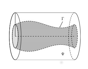
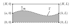
a	b

Figure 1: (a) The 3D fluid domain $\Psi=[0,H]\times[0,2\pi]\times[0,L]$ is radially symmetric and represented in cylindrical coordinates $(r,\theta,z)$. The open interface $\Gamma$ is a surface in the shape of an irregular tube that spans $\Psi$. (b) The 2D computational domain is a slice of the 3D domain where $\theta=0$ or $\Psi|_{\theta=0}=[0,H]\times[0,L]$. The computational slice contains an open immersed interface curve $\Gamma$. Note $\Gamma$ intersects the computational domain boundary at $(r,z)=(a,0)$ and $(r,z)=(b,L)$. $\mathbf{n}$ is the unit normal oriented towards the outside of the tube.

2.2 Boundary condition

Appropriate boundary conditions must be chosen to drive the fluid through the tube, which can be done by creating an axial pressure gradient inside the vessel. One way to accomplish this is to specify the value of pressure on the inlet and outlet of the tube using Dirichlet boundary conditions.

At the inlet, it is assumed that $w$ has a parabolic profile consistent with 3D Poiseuille flow. In 3D axisymmetric cylindrical coordinates, the pressure gradient and velocity are related by

$$w=-\frac{dp}{dz}\frac{1}{4\mu}(R^{2}-y^{2})$$ (1)

$$u=-\frac{dp}{dr}=0.$$ (2)

In the velocity decomposition method, boundary conditions must be imposed for both the Stokes and regular parts such that the boundary conditions for the full solution are still satisfied. The boundary conditions for the full solution are non-smooth for $w$ and discontinuous for $p$ at the inlet of the tube. The boundary conditions for the full solution are imposed on the Stokes part since $w_{s}$ is non-smooth and $p_{s}$ is discontinuous near the boundary. Homogeneous boundary conditions of the same type as the full solution are imposed for the regular solution. Below are the boundary conditions used for the two simulations in Section LABEL:sec:NSCylResults where the average inlet velocity is denoted $\bar{w}$.

• Inlet Boundary ($z=0$)

  $$p|_{z=0}=p_{s}|_{z=0}=\begin{cases}0&r>R\\ \frac{8\mu\bar{w}L}{R^{2}}&r\leq R\end{cases},$$ (3)

  $$w|_{z=0}=w_{s}|_{z=0}=\begin{cases}0&r>R\\ \frac{2\bar{w}(R^{2}-r^{2})}{R^{2}}&r\leq R\end{cases},$$ (4)

  $$u|_{z=0}=u_{s}|_{z=0}=0$$ (5)

  $$p_{r}|_{z=0}=u_{r}|_{z=0}=w_{r}|_{z=0}=0$$ (6)

• Outlet Boundary ($z=L$)

  $$p|_{z=L}=p_{s}|_{z=L}=p_{r}|_{z=L}=0$$ (7)

  $$\frac{\partial w}{\partial z}\Big{|}_{z=L}=\frac{\partial w_{s}}{\partial z}\Big{|}_{z=L}=\frac{\partial w_{r}}{\partial z}\Big{|}_{z=L}=0$$ (8)

  $$\frac{\partial u}{\partial z}\Big{|}_{z=L}=\frac{\partial u_{s}}{\partial z}\Big{|}_{z=L}=\frac{\partial u_{r}}{\partial z}\Big{|}_{z=L}=0$$ (9)

• Top Boundary ($r=H$)

  $$\frac{\partial p}{\partial r}\Big{|}_{r=H}=\frac{\partial p_{s}}{\partial r}\Big{|}_{r=H}=\frac{\partial p_{r}}{\partial r}\Big{|}_{r=H}=0$$ (10)

  $$\frac{\partial w}{\partial r}\Big{|}_{r=H}=\frac{\partial w_{s}}{\partial r}\Big{|}_{r=H}=\frac{\partial w_{r}}{\partial r}\Big{|}_{r=H}=0$$ (11)

  $$\frac{\partial u}{\partial r}\Big{|}_{r=H}=\frac{\partial u_{s}}{\partial r}\Big{|}_{r=H}=\frac{\partial u_{r}}{\partial r}\Big{|}_{r=H}=0$$ (12)

• Bottom Boundary ($r=0$)

  $$\frac{\partial p}{\partial r}\Big{|}_{r=0}=\frac{\partial p_{s}}{\partial r}\Big{|}_{r=0}=\frac{\partial p_{r}}{\partial r}\Big{|}_{r=0}=0$$ (13)

  $$\frac{\partial w}{\partial r}\Big{|}_{r=0}=\frac{\partial w_{s}}{\partial r}\Big{|}_{r=0}=\frac{\partial w_{r}}{\partial r}\Big{|}_{r=0}=0$$ (14)

  $$u|_{r=0}=u_{s}|_{r=0}=u_{r}|_{r=0}=0$$ (15)

2.3 Fluid structure interactions

The Navier-Stokes equations take the form

$$\rho\left(\frac{\partial\mathbf{u}}{\partial t}+\mathbf{u}\cdot\nabla\mathbf{u}\right) = \mu\Delta\mathbf{u}-\nabla p+\mathbf{F}$$ (16)

$$\nabla\cdot{\mathbf{u}} = 0$$ (17)

where ${\mathbf{u}}=(u,v,w)$, where $u$, $v$, and $w$ denote velocity components in the $r$-, $\theta$-, and $z$-directions, respectively, $p$ is the pressure, and $\mu$ is viscosity; and $\mathbf{F}$ is the interfacial force, which is singularly supported along $\Gamma$ (see below). We connsider also the zero Reynolds number regimes given by the Stokes equations:

$$\mu\Delta\mathbf{u}-\nabla p+\mathbf{F}=0$$ (18)

and the continuity equation (Eq. 17)

The force exerted by the interface $\Gamma$ can be written as

$${\bf F}({\bf x},t)=\int\displaylimits_{\Gamma}{\bf f}(\alpha)\delta({\bf x}-{\bf X}(\alpha))d\alpha,$$ (19)

where $\mathbf{X}$ denotes the position of the interface, $\alpha=\alpha(s,\theta,t)$ in 3D is the material coordinate(s) that parameterize the interface curve or surface at time $t$, ${\bf f}(\alpha)$ is the force strength at the point ${\bf X}(\alpha)$, and $\delta$ is the Dirac delta function. Since all 3D cases are axisymmetric, the interface is effectively a 2D curve, and it is sufficient to only consider $\alpha=\alpha(s,t)$.

The force strength from Eq. 19

$${\bf f}(\alpha)={\mathbf{f}}_{E}(\alpha)+{\mathbf{f}}_{T}(\alpha).$$ (20)

is comprised of a two major components: an elastic force ${\mathbf{f}}_{E}$ and a tether force ${\mathbf{f}}_{T}$. Since the interface has elastic properties, deviation from its resting configuration generates a restorative force. In 3D cylindrical coordinates, the elastic force derived in Ref.  ²⁴ is given by

$${\bf f}_{E}(s,t)=\frac{\partial T}{\partial\mathbf{\tau}}\mathbf{\tau}-2T\kappa\mathbf{n}$$ (21)

where $\kappa$ is the mean curvature and the tension $T(s,t)$ is given by

$$T(s,t)=a_{E}\left(\left|\frac{\partial{\bf X}}{\partial s}\right|-1\right)$$ (22)

In Eq. 22, $a_{E}$ controls the stiffness of the interface. In Eq. 21, the unit tangent vector to $\Gamma$ is given by

$$\tau(s,t)=\frac{\partial{\bf X}/\partial s}{\left|\partial{\bf X}/\partial s\right|}.$$ (23)

We assume that at steady state with the tethers at their equilibrium positions, tubular flow is that of Poiseuille flow, with fluid outside of the channel at rest. Thus, at steady state, one expects a jump discontinuity in p and in $u_{n}$ across $\Gamma$. To generate this steady-state flow profile, we assignn to the tether forces two components:

$${\mathbf{f}}_{T}={\mathbf{f}}_{T}^{0}+{\mathbf{f}}^{\prime}_{T}$$ (24)

where ${\mathbf{f}}_{T}^{0}$ is the force component needed to support Poiseuille flow along the channel (by generating the necessary jumps in the solution and its derivative).

The second component ${\mathbf{f}}_{T}^{\prime}$ arises from the displacement of the tethers from their equilibrium positions or anchor points. The interface control knots are tethered to anchor points in the fluid domain by a spring with resting length 0. Suppose the interface ${\mathbf{X}}$ is anchored to $\bar{{\mathbf{X}}}$. Let $a_{T}$ be the spring force constant. Then tether force is

$${\mathbf{f}}_{T}^{\prime}=a_{T}(\bar{{\mathbf{X}}}-{\mathbf{X}}).$$ (25)

If the interface knots move away from their anchor points, restorative forces are generated. Interface movement can either be restricted by using stationary anchor points or induced by moving the position of the anchor points in time.

The interface is deformable and is assumed to move at the same speed as the local fluid. The no-slip condition

$$\frac{d\mathbf{X}}{dt}=u(\mathbf{X}).$$ (26)

describes this motion.

2.4 Boundary conditions

Appropriate boundary conditions must be chosen to drive the fluid through the tube, which can be done by creating an axial pressure gradient in the vessel. One way to accomplish this is to specify the value of pressure on the inlet and outlet of the tube using Dirichlet boundary conditions. Another way is to impose inhomogeneous periodic boundary conditions. Specific boundary conditions used for the 2D and 3D cases simulations are discussed before the results.

Bi-periodic boundary conditions are imposed for velocity, which implies that the volume of the fluid in the tube remains constant in time. To drive flow, we prescribe a pressure gradient inside the tube, by requiring there to be a constant difference in pressure $P_{diff}$ at the inlet and outlet of the tube

$$p(0,y)=p(L,y)-\begin{cases}0&|y|\geq R\\ P_{diff}&|y|<R\end{cases}$$ (27)

where $R$ is the radius of the tube. The derivatives of pressure on the $x=0$ and $x=L$ boundaries are required to be equal

$$\frac{\partial p}{\partial x}|_{x=0}=\frac{\partial p}{\partial x}|_{x=L}.$$ (28)

This is referred to as an inhomogeneous periodic boundary condition. Not only does this create a pressure gradient in the tube, but it also forces the pressure gradient to be periodic, which is needed since periodic boundary conditions are imposed for velocity. Periodic boundary conditions are imposed for pressure at the $y=\pm H$ boundaries.

2.5 Derivation of jump conditions

The jump conditions for the Stokes equations and the Navier-Stokes equations are derived in Ref.  ²⁰ and Ref. ¹⁷ respectively for closed interfaces. Both the Stokes equations and the Navier-Stokes equations have the same jump conditions given the same interfacial forces ^{20, 17}. By creating a fictitious closed interface by adding segments to close the open tube interface, the same derivation for closed interfaces from Ref. ¹⁷ can be applied to open tube-shaped interfaces. This is shown in detail in Section 2.5 for the Stokes equations. The jump conditions for both the 3D Stokes and Navier-Stokes equations in cylindrical coordinates for both closed and open tube-shaped interfaces are

$$[p] =f_{n}$$ (29)

$$\left[\frac{\partial p}{\partial n}\right] =\frac{1}{r}\frac{\partial(rf_{s})}{\partial s}$$ (30)

$$\left[\mu\frac{\partial u}{\partial n}\right] =f_{s}\sin(\alpha)$$ (31)

$$\left[\mu\frac{\partial w}{\partial n}\right] =-f_{s}\cos(\alpha)$$ (32)

where $\alpha$ is the angle between the normal and $r$ direction ^{20, 17}.

Next, we derive the jump conditions across an open tube for the 3D Stokes equations in axisymmetric cylindrical coordinates. We show that the jump conditions in cylindrical coordinates for an interface that is in the shape of an open tube have the same dependence on force and interface position as in the closed tube case.

Again, the interface must be shaped like a closed surface for the derivation. Therefore, consider the fictitious closed surface

$$\Gamma_{c}=\Gamma\cup\{(r,\theta,0)|r\in[0,a],\theta\in[0,2\pi]\}\cup\{(r,\theta,L)|r\in[0,b],\theta\in[0,2\pi]\}$$ (33)

which is formed by the interface $\Gamma$ and the inlet and outlet of the tube which intersect the fluid domain $\Psi$ at $z=0$ and $z=L$ respectively.

Let $\Omega_{\epsilon}$ be an extended domain that contains the surface interface $\Gamma_{c}$ where the distance between $\Omega_{\epsilon}$ and $\Gamma_{c}$ shrinks to zero as $\epsilon$ approaches zero. Note that $\Omega_{\epsilon}$ extends outside of the original fluid domain $\Psi$.

Although symmetry is imposed later, first consider the fully 3D Stokes equations in cylindrical coordinates, given by

$$\frac{\partial p}{\partial r}=\mu\left(\Delta-\frac{1}{r^{2}}\right)u-\frac{2\mu}{r^{2}}\frac{\partial v}{\partial\theta}+\hat{F_{1}}$$ (34)

$$\frac{1}{r}\frac{\partial p}{\partial\theta}=\mu\left(\Delta-\frac{1}{r^{2}}\right)v+\frac{2\mu}{r^{2}}\frac{\partial u}{\partial\theta}+\hat{F_{2}}$$ (35)

$$\frac{\partial p}{\partial z}=\mu\Delta w+\hat{F_{3}}$$ (36)

$$\frac{1}{r}\frac{\partial(ru)}{\partial r}+\frac{1}{r}\frac{\partial v}{\partial\theta}+\frac{\partial w}{\partial z}=0$$ (37)

where $\mathbf{x}=(r,\theta,z)$, $u$, $v$, and $w$ are the velocities in the $r$, $\theta$, and $z$ directions respectively, and $\mathbf{\hat{F}}=(\hat{F_{1}},\hat{F_{2}},\hat{F_{3}})$ with

$$\hat{F_{i}}=\iint_{\Gamma_{c}}\hat{f}_{i}(s,\theta,t)\delta(\mathbf{x}-\mathbf{X}(s,\theta,t))dS$$ (38)

for $i=1,2,3$, where $\mathbf{\hat{f}}$ is the extension of $\mathbf{f}$ which is supported on $\Gamma$ and agrees with $\mathbf{f}$ on $\Gamma$. Even if the correction terms are computed for the fictitious closed domain $\Gamma_{c}$ there is no contribution from the extensions of the interface. Therefore, the hat symbol is dropped for the rest of the derivation. Now the derivation mirrors the procedure found in Ref. ²⁰.

Taking the divergence of Eqs. 34, 35, and 36 gives Poisson’s equation for pressure

$$\Delta p=\nabla\cdot\mathbf{F}.$$ (39)

Let $\phi(r,\theta,z)$ be an arbitrary twice continuously differentiable test function. Multiply the left hand side of Eq. 39 by $\phi$ and integrate over $\Omega_{\epsilon}$

$$\iiint_{\Omega_{\epsilon}}\Delta p\phi dV =\iint_{\partial\Omega_{\epsilon}}\phi(\nabla p\cdot\mathbf{n})dS-\iiint_{\Omega_{\epsilon}}\nabla\phi\cdot\nabla pdV$$ (40)

$$=\iint_{\partial\Omega_{\epsilon}}\phi(\nabla p\cdot\mathbf{n})dS-\left(\iint_{\partial\Omega_{\epsilon}}(\nabla\phi\cdot\mathbf{n})pdS-\iiint_{\Omega_{\epsilon}}(\Delta\phi)pdV\right)$$ (41)

$$\to\iint_{\Gamma_{c}}\phi\left[\frac{\partial p}{\partial\mathbf{n}}\right]dS-\iint_{\Gamma_{c}}\frac{\partial\phi}{\partial\mathbf{n}}[p]dS+0\textrm{ as }\epsilon\to 0.$$ (42)

The first and second lines are by Green’s first Identity and the divergence theorem, respectively. The last line is found by taking the limit as $\epsilon$ goes to zero. The last term goes to zero since pressure is bounded. The surface element is $dS=rdsd\theta$. By imposing the axisymmetric assumptions on $p$ and $\phi$ we get that

$$\iiint_{\Omega_{\epsilon}}\Delta p\phi dV\to 2\pi\left(\int_{\Gamma_{c}}\phi\left[\frac{\partial p}{\partial\mathbf{n}}\right]rds-\int_{\Gamma_{c}}\frac{\partial\phi}{\partial\mathbf{n}}[p]rds\right),$$ (43)

where $\Gamma_{c}$ denotes the curve formed by restricting the surface $\Gamma_{c}$ to a fixed $\theta$. Multiply the right hand side of Eq. 39 by $\phi$ and integrate over $\Omega_{\epsilon}$.

$$\iiint_{\Omega_{\epsilon}}(\nabla\cdot\mathbf{F})\phi(\mathbf{x})dV =\iiint_{\Omega_{\epsilon}}\left(\iint_{\Gamma_{c}}\nabla\cdot\left(\mathbf{f}(s,\theta,t)\delta(\mathbf{x}-\mathbf{X}(s,\theta,t))\right)dS\right)\phi(\mathbf{x})dV$$ (44)

$$=\iint_{\Gamma_{c}}\mathbf{f}(s,\theta,t)\left(\iiint_{\Omega_{\epsilon}}\nabla\cdot\delta(\mathbf{x}-\mathbf{X}(s,\theta,t))\phi(\mathbf{x})dV\right)dS$$ (45)

$$=-\iint_{\Gamma_{c}}\mathbf{f}(s,\theta,t)\cdot\nabla\phi(\mathbf{x})dS$$ (46)

The last line is found using the divergence theorem and noting that the $\delta(\mathbf{x}-\mathbf{X}(s,\theta,t))$ has support on $\Gamma_{c}$ and is zero on $\partial\Omega_{\epsilon}$. Applying the axisymmetric assumption that $\phi$ and $f$ are independent of $\theta$ to Eq. 46 yields

$$\iiint_{\Omega_{\epsilon}}(\nabla\cdot\mathbf{F})\phi(\mathbf{x})dV =-2\pi\int_{\Gamma_{c}}\left(f_{1}\frac{\partial\phi}{\partial r}+f_{3}\frac{\partial\phi}{\partial z}\right)rds$$ (47)

$$=-2\pi\int_{\Gamma_{c}}\left(f_{n}\frac{\partial\phi}{\partial n}+f_{s}\frac{\partial\phi}{\partial s}\right)rds$$ (48)

$$=-2\pi\int_{\Gamma_{c}}\left(f_{n}r\frac{\partial\phi}{\partial n}-\frac{\partial f_{s}}{\partial s}\phi\right)ds$$ (49)

where $\Gamma_{c}$ denotes the curve formed by restricting $\Gamma_{c}$ to a fixed $\theta$. The second line is found by breaking the force into components normal and tangential to the interface. The last line is found using integration by parts. Since $\phi$ is arbitrary, we have

$$[p] =f_{n}$$ (50)

$$\left[\frac{\partial p}{\partial n}\right] =\frac{1}{r}\frac{\partial(f_{s}r)}{\partial s}.$$ (51)

To find the jump conditions for $u$, multiply Eq. 34 by $\phi$ and integrate

$$\iiint_{\Omega_{\epsilon}}\phi\frac{\partial p}{\partial r}dV=\iiint_{\Omega_{\epsilon}}\phi\mu\Delta udV-\iiint_{\Omega_{\epsilon}}\phi\frac{\mu u}{r^{2}}dV+\iint_{\Gamma_{c}}f_{1}\phi dS.$$ (52)

The first term on the right hand side of the Eq. 52 approaches the following as $\epsilon\to 0:$

$$\iiint_{\Omega_{\epsilon}}\phi\mu\Delta udV =\iint_{\partial\Omega_{\epsilon}}\phi\mu(\nabla u\cdot\mathbf{n})dS-\iiint_{\Omega_{\epsilon}}\mu\nabla\phi\cdot\nabla udV$$ (53)

$$\to\iint_{\Gamma_{c}}\phi\left[\mu\frac{\partial u}{\partial\mathbf{n}}\right]dS-0$$ (54)

The second term on the right hand side of the Eq. 52

$$\iiint_{\Omega_{\epsilon}}\phi\frac{\mu u}{r^{2}}dV=\iiint_{\Omega_{\epsilon}}\phi\frac{\mu u}{r^{2}}rdrd\theta dz=\iiint_{\Omega_{\epsilon}}\phi\frac{\mu u}{r}drd\theta dz$$ (55)

approaches 0 as $\epsilon\to 0$. This is true because by the axisymmetric condition when $r\to 0$, $u$ approaches zero. Additionally $\lim_{r\to 0}\frac{u}{r}=\frac{\partial u}{\partial r}$, which is finite.

The first term on the left hand side of the Eq. 52 approaches the following as $\epsilon\to 0$.

$$\iiint_{\Omega_{\epsilon}}\phi\frac{\partial p}{\partial r}dV =\iiint_{\Omega_{\epsilon}}\phi\nabla\cdot[p,0]-\frac{p}{r}dV$$ (56)

$$\to\iint_{\Gamma_{c}}\phi[p]\cos(\alpha)dS+0$$ (57)

where $\alpha$ is the angle between the normal and $r$ direction. Therefore

$$\left[\mu\frac{\partial u}{\partial n}\right]=[p]\cos(\alpha)-\frac{f_{1}}{|f_{1}|}=f_{s}\sin(\alpha).$$ (58)

Similarly,

$$\left[\mu\frac{\partial w}{\partial n}\right]=[p]\sin(\alpha)-\frac{f_{3}}{|f_{3}|}=f_{s}\cos(\alpha).$$ (59)

3 Numerical method

To solve the immersed boundary problem, we compute the fluid velocity and pressure on a fixed Eulerian grid. A moving Lagrangian frame of reference is used to track the location of the interface $\Gamma$ over time. In 2D, the Stokes equations are solved on the fluid computational grid,

$$\Omega_{h}=\left\{\mathbf{x}_{i,j}=\left(jh,ih-\frac{H}{2}\right)|i\in{1,\dots,N_{y}}\textrm{ and }j\in{1,\dots,N_{x}}\right\}$$

where $h$ is the grid spacing and $N_{x}=\frac{L}{h}+1$ and $N_{y}=\frac{H}{h}+1$ are the number of grid points in the $x$ and $y$ directions respectively. In 3D, the Stokes equations are solved on the fluid computational grid,

$$\Omega_{h}=\left\{\mathbf{x}_{i,j}=\left(ih,jh-\frac{H}{2}\right)|i\in{1,\dots,N_{r}}\textrm{ and }j\in{1,\dots,N_{z}}\right\}$$

where $h$ is the grid spacing and $N_{r}=\frac{H}{h}+1$ and $N_{z}=\frac{L}{h}+1$ are the number of grid points in the $r$ and $z$ directions respectively. In both the 2D and 3D case, the interface position at time $t_{n}=n\Delta t$ is tracked by $N_{b}$ boundary markers $\mathbf{X}^{n}=\{\mathbf{X}_{i}^{n}\}_{i=1}^{N_{b}}$ that are connected by a cubic spline.

3.1 Velocity decomposition method

The velocity decomposition method, developed by Ref.  ²⁵, can be used to avoid computing most of the correction terms that are needed for the immersed interface method for the Navier-Stokes equations. This method leverage the fact that, given the same singular interfacial force, the jumps in the solutions are identical for both the Stokes equations and the Navier-Stokes equations as shown by Ref.  ¹³ and Ref.  ¹⁴ respectively. This result occurs because the no-slip condition implies that velocity and its material derivative are continuous at the interface ²⁶.

It is sufficient to break the solution of the Navier-Stokes equations into a part that satisfies the Stokes equations with the singular interfacial forces and a regular part that solves the remaining equations as shown below.

Suppose $\mathbf{u}$ and $p$ solve the Navier-Stokes equations with a singularly-supported interfacial force $\mathbf{F}$. Let

$$\mathbf{u}=\mathbf{u}_{s}+\mathbf{u}_{r}$$ (60)

$${p}={p_{s}}+{p_{r}}$$ (61)

where the subscripts $s$ and $r$ are used for the Stokes and regular part, respectively. The Stokes part, $\mathbf{u}_{s}$ and $p_{s}$, satisfies the Stokes equations with the interfacial force $\mathbf{F}$

$$-\mu\Delta\mathbf{u_{s}}=-\nabla p_{s}+\mathbf{F}$$ (62)

$$\nabla\cdot\mathbf{u}_{s}=0.$$ (63)

The regular part, $\mathbf{u}_{r}$ and $p_{r}$, satisfies the remaining terms in the full Navier-Stokes equations

$$\rho\left(\frac{\partial\mathbf{u}_{r}}{\partial t}+\mathbf{u}\cdot\nabla\mathbf{u}_{r}\right)=\mu\Delta\mathbf{u_{r}}-\nabla p_{r}+\mathbf{F_{b}}$$ (64)

$$\nabla\cdot\mathbf{u}_{r}=0$$ (65)

where

$$\mathbf{F}_{b}=-\rho\left(\frac{\partial\mathbf{u}_{s}}{\partial t}+\mathbf{u}\cdot\nabla\mathbf{u}_{s}\right).$$ (66)

The Stokes part is found first, so $\mathbf{F}_{b}$ is known and treated as a body force when solving for the regular part. The force $\mathbf{F}_{b}$ is a continuous function in the fluid domain since $\mathbf{u}_{s}$ and its material derivative are continuous. Notice that the full velocity $\mathbf{u}$ is used in the transport of $\mathbf{u}_{r}$ and in $\mathbf{F}_{b}$.

This method has several advantages over the immersed interface method for the Navier-Stokes equations. First, correction terms only need to be computed for the Stokes part of the solution, saving considerable time in implementation since numerous correction terms are needed for the additional terms in the Navier-Stokes equations. Secondly, the velocity decomposition method can also be implemented with fractional time steps that help overcome some of the challenges of simulating stiff interfaces. Small fractional time steps are used to move the interface, which is done by only computing the velocity on the interface. This computation is done using Stokeslets to compute the Stokes part of the velocity at the interface and interpolating the regular part of velocity on the interface in time ²⁵. Therefore, the interface position can be updated without computing the full solution at each fractional time step.

3.2 Stokes part: immersed interface method for open tube interfaces

The Stokes part of the equation is solved using the IIM-OT. This method requires the jump conditions for the solution to be known a priori. The velocity decomposition method is based on the fact that the jump conditions for the Navier-Stokes equations and the Stokes equations with the same interfacial forces are identical ²⁵, which is true because the no-slip condition implies that

$$[\mathbf{u}]=0$$ (67)

since the interface moves at the velocity of the local fluid ²⁶. Taking the material derivative of velocity gives

$$\left[\frac{\partial\mathbf{u}}{\partial t}+\nabla\mathbf{u}\cdot\mathbf{u}\right]=0.$$ (68)

Therefore, the advection term does not contribute to the jump conditions ²⁶.

Since the jump conditions are known, the immersed interface method for open tube interfaces needs to only correct the incompressible Stokes equations. First, the incompressible Stokes equations are converted into a series of uncoupled Poisson problems. The Poisson problem for pressure, $p_{s}$ is found by taking the divergence of Eq. 62 and use the incompressibility condition

$$\nabla\cdot(-\mu\Delta\mathbf{u_{s}})=-\nabla\cdot(\nabla p_{s})+\nabla\cdot\mathbf{F}$$ (69)

$$\Delta p_{s}=\nabla\cdot\mathbf{F}.$$ (70)

Once $p_{s}$ is known, Eq. 62 reduces to a Poisson problem for each component of velocity, $\mathbf{u}_{s}$. Therefore, to solve the Stokes part it is sufficient to use the immersed interface method for Poisson problems.

The immersed interface method for Poisson problems was developed by Ref.  ¹². The Poisson problems are discretized using the finite difference method. Therefore, to apply the IIM-OT to the Stokes equations, it is only necessary to compute the corrections terms for the first- and second-order spatial derivatives. Once the jump conditions for the open tube interface are known, the correction terms can be computed using the immersed interface method for Poisson problems.

3.3 Regular part: projection method and semi-Lagrangian method

The regular part of the solution satisfies Eqs. 64–66. The advection terms and the body force $\mathbf{F}_{b}$ are discretized using the backward difference formula, where the upstream values of velocity are found using the semi-Lagrangian method. A projection method is used to enforce the incompressibility condition.

3.3.1 Semi-Lagrangian method

The advection terms, $\frac{\partial\mathbf{u}_{r}}{\partial t}+\mathbf{u}\cdot\nabla\mathbf{u}_{r}$ and $\frac{\partial\mathbf{u}_{s}}{\partial t}+\mathbf{u}\cdot\nabla\mathbf{u}_{s}$, can be thought of as material derivatives or the derivatives along the path of a fluid particle. In the semi-Lagrangian method, the material derivative is computed at Eulerian grid points, which combines the Lagrangian and Eulerian variable frameworks and has several benefits over a purely Lagrangian or Eulerian framework.

The material derivative is computed at Eulerian grid points. Therefore, the resolution of the grid does not deteriorate or get distorted with the fluid flow, which can occur in Lagrangian methods.

Particles cannot physically cross the impermeable immersed interface so that the material derivatives will be smooth, which reduces the number of correction terms needed in the immersed interface method. For example, correction terms would be needed for the time derivatives computed on an Eulerian grid when the interface crosses over a grid point in a time step. Additionally, $\nabla\mathbf{u}$ is discontinuous at $\Gamma$, so the terms, $\mathbf{u}\cdot\nabla\mathbf{u}_{r}$ and $\mathbf{u}\cdot\nabla\mathbf{u}_{s}$, would need to be corrected near the interface if discretized on the Eulerian grid ^{27, 28}. Additionally, the nonlinear terms of the Navier-Stokes equations do not need to be discretized explicitly in the semi-Lagrangian method.

The semi-Lagrangian method is used to compute the velocity along the path of a fluid particle that passes through the grid point $\mathbf{x^{n+1}}$ at time $t_{n+1}$, which is used to compute the material derivative of the velocity of the particles. This is done by first computing the upstream positions of the particle, $\mathbf{x^{n}}$ and $\mathbf{x^{n-1}}$, at two previous times, $t_{n}$ and $t_{n-1}$, respectively. An example of a 1D particle path is shown in Fig. LABEL:fig:particlePath.

The upstream position of the particle located on the Eulerian fluid grid point, $\mathbf{x}_{0}$, at time $t_{n+1}$ can be found by integrating

$$\frac{d\mathbf{x}(t)}{dt}=\mathbf{u}(\mathbf{x}(t),t),\quad\mathbf{x}(t_{n+1})=\mathbf{x}_{0},$$ (71)

backwards in time. The predictor-corrector method

$$\mathbf{x}^{*} =x_{0}-\frac{\Delta t}{2}\mathbf{u}\left(\mathbf{x}_{0}-\frac{\Delta t}{2}\mathbf{u}^{n+\frac{1}{2}},t_{n+\frac{1}{2}}\right)$$ (72)

$$\mathbf{x}^{n} =\mathbf{x}_{0}-\Delta t\mathbf{u}(\mathbf{x}^{*},t_{n+\frac{1}{2}})$$ (73)

and

$$\mathbf{x}^{*} =x_{0}-\Delta t\mathbf{u}\left(\mathbf{x}_{0}-\Delta t\mathbf{u}^{n},t_{n}\right)$$ (74)

$$\mathbf{x}^{n-1} =\mathbf{x}_{0}-2\Delta t\mathbf{u}(\mathbf{x}^{*},t_{n})$$ (75)

can be used to find the upstream positions at two previous time steps with second-order temporal accuracy. Notice that $\mathbf{u}^{n+\frac{1}{2}}$ is approximated using the time extrapolation $\frac{3}{2}\mathbf{u}^{n}-\frac{1}{2}\mathbf{u}^{n-1}$.

It is unlikely that the upstream positions coincide with grid points. Therefore the velocity at upstream values

$$\mathbf{\tilde{u}}_{r}^{n} =\mathbf{u}_{r}(\mathbf{x}^{n},t_{n})$$ (76)

$$\mathbf{\tilde{u}}_{r}^{n-1} =\mathbf{u}_{r}(\mathbf{x}^{n-1},t_{n-1})$$ (77)

are interpolated in space from the velocity at grid points using cubic Lagrangian interpolation. This interpolation has 4th order accuracy in space. Once the upstream values of velocity are known, the material derivative is found using the second-order backwards difference formula. Therefore, Eq. 64 can be discretized using

$$\frac{3\mathbf{u}_{r}^{n+1}-4\mathbf{\tilde{u}}_{r}^{n}+\mathbf{\tilde{u}}_{r}^{n-1}}{2\Delta t}+\nabla p_{r}^{n}=\mu\Delta\mathbf{u}^{n+1}_{r}+\mathbf{F}^{n+1}_{b}.$$ (78)

3.3.2 Projection method

The coupling of the velocity components and pressure in the Navier-Stokes equations would create a large finite difference system if all components were solved simultaneously. Instead, the projection method is used to solve the regular part. In this procedure, an intermediate value of velocity ${\bf u}^{*}$ and pressure $p^{*}$ are found that satisfy

$$\frac{D{\bf u^{*}}}{Dt}=-\nabla p^{*}+\mu\nabla^{2}{\bf u^{*}}+{\bf F}.$$ (79)

The intermediate values are then projected, $P({\bf u}^{*})={\bf u}$, into the subspace of divergence-free vector fields so that $\nabla\cdot{\bf u}=0.$ This works because every vector field $\mathbf{w}$ can be written as a Hodge decomposition $\mathbf{w}=\mathbf{v}+\nabla\phi$ where $\mathbf{v}$ is divergence-free. This projected value $\mathbf{u}$ satisfies the Navier-Stokes equations.

The regular part of the Navier-Stokes equations can be numerically solved using the following projection method. An intermediate velocity value, ${\bf u}^{*}$ is found by solving

$$\frac{3\mathbf{u}_{r}^{*}-4\mathbf{\tilde{u}}_{r}^{n}+\mathbf{\tilde{u}}_{r}^{n-1}}{2\Delta t}+\nabla p_{r}^{n}=\mu\Delta\mathbf{u}^{*}_{r}+\mathbf{F}^{n+1}_{b}.$$ (80)

where $p_{r}^{n}$ is the value of pressure from the previous time step. The intermediate value $\mathbf{u}^{*}_{r}$ is approximately projected into divergence-free space by defining $\phi$ as

$$\mathbf{u}_{r}^{n+1}=\mathbf{u}^{*}_{r}-(\Delta t)\nabla\phi^{n+1},$$ (81)

which can be found by solving

$$\Delta\phi^{n+1} =\frac{1}{\Delta t}\nabla\cdot{\bf u}_{r}^{*}.$$ (82)

Then, velocity and the gradient of pressure can be found by

$${\bf u}_{r}^{n+1}={\bf u}_{r}^{*}-\Delta t\nabla\phi^{n+1}$$ (83)

$$\nabla p_{r}^{n+1}=\nabla p^{n}+\frac{3}{2}\nabla\phi^{n+1}-\mu\Delta t\nabla^{3}\phi^{n+1}.$$ (84)

3.4 Time-stepping

The interface movement is govern by Eq. LABEL:eq:noSlip. Suppose the interface position at time $t_{n}=n\Delta t$ is represented by $N_{b}$ boundary markers $\mathbf{X}^{n}=\{\mathbf{X}_{i}^{n}\}_{i=1}^{N_{b}}$. The velocity at each marker $\mathbf{U}^{n}=\{\mathbf{U}_{i}^{n}\}_{i=1}^{N_{b}}$ can be found by interpolating the velocity from the fluid grid to the markers using a second-order method such as bi-linear interpolation. Care must be taken during this interpolation since the velocity near the interface is not smooth. The velocity could be corrected near the interface or a one-sided approximation for velocity could be used where all interpolation points are on the same side of the interface.

For the time stepping to be second-order, the velocity on the interface at two previous time levels, $\mathbf{U}^{n}$ and $\mathbf{U}^{n-1}$, are needed. The interface position is then updated as follows:

$$\mathbf{X}^{n+1}=\mathbf{X}^{n}+\Delta t\left(\frac{3}{2}\mathbf{U}^{n}-\frac{1}{2}\mathbf{U}^{n-1}\right).$$ (85)

To move the interface initially, forward Euler’s method was used.

3.5 Velocity decomposition method algorithm outline

At time $t_{n}$, the following are known: $\mathbf{u}^{i}$, $p^{i}$, $\mathbf{u}_{s}^{i}$, $p_{s}^{i},$ $\mathbf{u}_{r}^{i}$, $p_{r}^{i},$ and ${\bf X}^{i}$ for $i=n$ and $i=n-1$. The following procedure can be used to compute the solution at $t_{n+1}$.

1. Update interface position $\mathbf{X}^{n+1}$.

   1. Interpolate velocity at the interface $\mathbf{U}^{i}$ from fluid grid $\mathbf{u}^{i}$ using

      $$\mathbf{U}^{n}\approx\mathbf{u}^{n}(\mathbf{X}^{n},t_{n})$$ (86)

   2. The interface positions ${\bf X}^{n+1}$ is updated using the no slip condition

      $$\mathbf{X}^{n+1}=\mathbf{X}^{n}+\Delta t\left(\frac{3}{2}\mathbf{U}^{n}-\frac{1}{2}\mathbf{U}^{n-1}\right).$$ (87)

   3. Compute the interfacial force $\mathbf{f}^{n+1}$ from the interface position $\mathbf{X}^{n+1}$.

2. Compute the Stokes solution, $\mathbf{u}^{n+1}_{s}$ and $p^{n+1}_{s}$.

   1. Use force $\mathbf{f}^{n+1}$ to find the correction terms, $\mathbf{C}^{n+1}_{p_{h}}$ and $\mathbf{C}^{n+1}_{\mathbf{u}_{h}}$, for pressure and velocity respectively using the immersed interface method.

   2. Solve the following Poisson problem for pressure, $p^{n+1}$:

      $$\Delta_{h}p^{n+1}=\mathbf{C}^{n+1}_{p_{h}}$$

   3. Compute the discrete pressure gradient, $\nabla_{h}p^{n+1}$ using correction terms.

   4. Solve the following Poisson problems for each component of velocity, $\mathbf{u}^{n+1}$.

      $$\Delta_{h}\mathbf{u}^{n+1}=-\nabla_{h}p^{n+1}+\mathbf{C}^{n+1}_{\mathbf{u}_{h}}$$

3. Compute regular solution, $\mathbf{u}^{n+1}_{r}$ and $p^{n+1}_{r}$.

   1. Use semi-Lagrangian method to compute $F_{b}=-\frac{d{\bf u}_{s}}{dt}$, $\mathbf{\tilde{u}}_{r}^{n}$, and $\mathbf{\tilde{u}}_{r}^{n-1}.$

   2. Solve momentum equation for intermediate regular velocity, $\mathbf{u}^{*}$.

   3. Compute $\phi^{n+1}$ needed to project into divergent-free space.

   4. Find $\mathbf{u}^{n+1}_{r}$ and $p_{r}^{n+1}$ using $\phi^{n+1}$.

4. Compute the full solution at time $t_{n+1}$ by adding the Stokes and regular part.

Forward Euler’s method is used for the first step of the time stepping methods. The local truncation error is $O(\Delta t^{2})$ and this is only used for one time step, second-order temporal accuracy is still maintained.

4 Numerical results

4.1 Stokes Results

A grid refinement study was conducted to test the spatial convergence rate for the immersed interface method in an open tube for the Stokes equations in 3D axisymmetric cylindrical coordinates shown in Eqs. 88 – 90. In this test, the tube was displaced and allowed to return to its resting position as a tube with a constant radius. In addition to confirming the order of the method, this test also aims to validate that approximate 3D Poiseuille flow is achieved when the tube has near constant radius.

$$\frac{\partial p}{\partial r}=\mu\left(\frac{1}{r}\frac{\partial}{\partial r}\left(r\frac{\partial w}{\partial r}\right)+\frac{\partial^{2}w}{\partial z^{2}}-\frac{w}{r^{2}}\right)$$ (88)

$$\frac{\partial p}{\partial z}=\mu\left(\frac{1}{r}\frac{\partial}{\partial r}\left(r\frac{\partial u}{\partial r}\right)+\frac{\partial^{2}u}{\partial z^{2}}\right)$$ (89)

$$\frac{1}{r}\frac{\partial(ru)}{\partial r}+\frac{\partial w}{\partial z}=0$$ (90)

For the cylindrical coordinate test cases, the domain is assumed to be radially symmetric. This allows three dimensional kinetics with two dimensional computational costs. Although, the fluid domain is $\Omega=[-1.625\text{cm},1.625\text{cm}]\times[0,2\pi]\times[0\text{cm},4.25\text{cm}]$, the solution is only computed on the computational domain $\Omega=[0\text{cm},1.625\text{cm}]\times[0\text{cm},4.25\text{cm}]$ which is the $\theta=0$ slice of the fluid domain. $R=.7$ cm is the resting radius of the tube.

For this case, the interface was initially displaced in the $r$ direction according to the function

$$r(z)=.2e^{-(z-\frac{L}{2})^{2}}-.2e^{-(\frac{L}{2})^{2}}+R$$ (91)

where $R$ is the resting radius of the tube. The interface was then allowed to return to its resting position as a straight tube.

Flow is driven through the tube by prescribing a pressure gradient over the computational domain using Dirichlet boundary conditions. At the inlet, it is assumed that $w$ has a parabolic profile consistent with 3D Poiseuille flow. In 3D axisymmetric cylindrical coordinates, the pressure gradient and velocity are related by

$$w=-\frac{dp}{dz}\frac{1}{4\mu}(R^{2}-y^{2})$$ (92)

$$u=-\frac{dp}{dr}=0.$$ (93)

• Inlet Boundary ($z=0$)

  $$p|_{z=0}=\begin{cases}0&|r|<R\\ \frac{8\mu\bar{w}L}{R^{2}}&|r|\leq R\end{cases},\quad\quad w|_{z=0}=\begin{cases}0&r<-R\\ \frac{2\bar{w}(R^{2}-r^{2})}{R^{2}}&|r|\leq R\\ 0&R<r\end{cases},\quad\quad u|_{z=0}=0$$

• Outlet Boundary ($z=L$)

  $$p|_{z=L}=0,\quad\quad\frac{\partial w}{\partial z}|_{z=L}=0,\quad\quad\frac{\partial u}{\partial z}|_{z=L}=0$$

• Top Boundary ($r=H$)

  $$\frac{\partial p}{\partial r}|_{r=H}=0,\quad\quad\frac{\partial w}{\partial r}|_{r=H}=0,\quad\quad\frac{\partial u}{\partial r}|_{r=H}=0$$

• Bottom Boundary ($r=0$)

  $$\frac{\partial p}{\partial r}|_{r=0}=0,\quad\quad\frac{\partial w}{\partial r}|_{r=0}=0,\quad\quad u|_{r=0}=0$$

The remainder of the parameters used for this experiment are shown in Table 1.

Table 1: Parameters used for the spatial convergence study of the IIM-OT for 3D Stokes flow in axisymmetric cylindrical coordinates.

Parameter	Symbol	Value
Viscosity	$\mu$	0.1 gm/(cm$\cdot$s)
Density	$\rho$	1 gm/cm3
Domain length	$L$	4.25 cm
Domain height	$H$	1.625 cm
Initial tube radius	$R$	0.7 cm
Interface control points	$N_{b}$	100
Simulation length	$T$	4 s
Time steps	$N_{t}$	2000
Time step size	$\Delta t$	2e-3 s
Tether force constant	$a_{Tether}$	10 gm/s2
Elastic force constant	$a_{Elastic}$	.1 gm/s2
Average Inlet Velocity	$\bar{w}$	1 cm/s

The solution was computed at various resolutions and then compared to a $1089\times 417$ high-resolution solution. The results of the convergence study shown in Table 2 indicate that the method is second-order accurate in space.

Table 2: Spatial convergence results of the IIM-OT for Stokes flow in cylindrical coordinates. Solutions are compared to a high resolution, $1089\times 417$ solution at time $t=0$.

Grid Size		p		w		u
$N_{z}$	$N_{r}$	$||\cdot||_{\infty}$	Order	$||\cdot||_{\infty}$	Order	$||\cdot||_{\infty}$	Order
35	14	0.03741		0.25162		0.10789
69	27	0.00796	2.23	0.10349	1.28	0.02643	2.03
137	53	0.00189	2.07	0.01862	2.47	0.00628	2.07
273	105	0.00044	2.12	0.00456	2.03	0.00145	2.12
545	209	0.00008	2.37	0.00027	4.07	0.00029	2.34

Fig. 3 shows the interface position overlaid on a quiver plot that show the velocity as an arrow with components $(w,u)$ various times. Since the most dramatic changes occur in the beginning of the simulation, the Fig. 2(a), 2(b), and 3(a) show the results at $t=0$, $t=.05s$, and $t=.1s$ respectively. Recall that because of the no-slip condition on the interface, the interface moves at the local fluid velocity. Therefore, the velocity slope field in Fig. 2(a) indicates that the interface is moving towards its resting position as a straight tube (shown in Fig. 3(b)). Initially in Fig. 2(a), some of the fluid is pushed to the left towards the proximal end of the tube as the interface relaxes. As the interface gets closer to its resting configuration, it exerts less force on the fluid. Therefore, in Figs. 2(b)–3(b), all fluid in the tube moves to the right towards the distal end of the tube. Fig. 3(b) shows the resting position of the interface, in which the velocity exhibits a parabolic profile inside the interface and dissipates to zero outside of the interface.

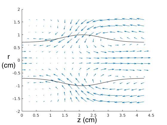
((a)) The interface position and velocity quiver plot at $t=0$ s shows the interface is moving towards $r=\pm 0.7$ cm.

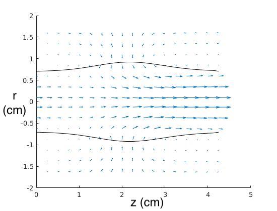
((b)) The interface position and velocity quiver plot at $t=0.05$ s shows the interface is moving towards $r=\pm 0.7$ cm.

Figure 2: The interface (black line) is shown at various times as it relaxes from its displaced in the axisymmetric cylindrical computational domain. The interface position is superimposed on a quiver plot that show the velocity as an arrow with components $(w,u)$.

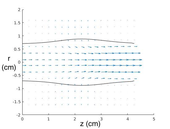
((a)) The interface position and velocity quiver plot at $t=0.1$ s shows the interface is moving towards $r=\pm 0.7$ cm.s

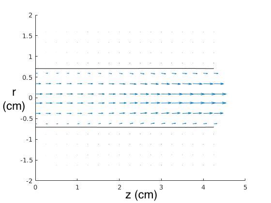
((b)) The interface position and velocity quiver plot at $t=2$ s shows the interface at its resting position where $r=\pm 0.7$ cm.

Figure 3: The interface (black line) is shown at various times as it relaxes from its displaced in the axisymmetric cylindrical computational domain. The interface position is superimposed on a quiver plot that show the velocity as an arrow with components $(w,u)$.

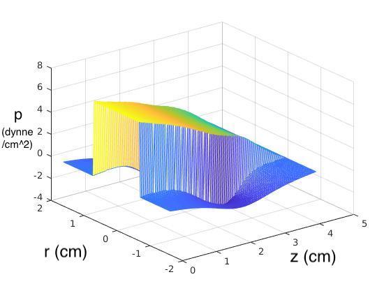
((a)) The initial pressure in the computational domain at $t=0$s.

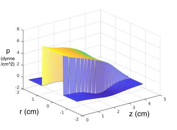
((b)) The pressure at $t=0.05$ s as the interface is returning to its resting position.

Figure 4: Pressure in the axisymmetric cylindrical computational domain at various times as the interface relaxes from its displaced position to rest.

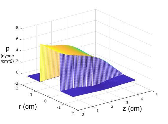
((a)) The pressure at $t=0.1$ s as the interface is returning to its resting position.

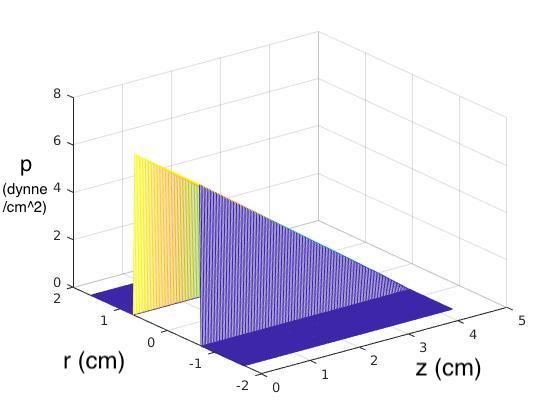
((b)) The pressure is linearly decreasing inside the tube and zero outside at $t=2$s when the interface is in its resting position.

Figure 5: Pressure in the axisymmetric cylindrical computational domain at various times as the interface relaxes from its displaced position to rest.

The pressure in the computational domain at $t=0$s, $t=.05$s, $t=.1$s and $t=2$s are shown in Fig. 5. The IIM-OT captures the discontinuity in pressure across the interface as can be seen in Fig. 5. Additionally, pressure decreases along the length of the domain inside of the interface, which creates a pressure gradient that drives fluid through the open tube. Another pressure gradient outside of the tube can be seen in Fig. 4(a) which drives the fluid to restore the interface to its resting position. Finally, Fig. 5(b) shows a linearly decreasing pressure that is typical of Poiseuille flow in a cylinder.

4.2 Navier-Stokes Equations

4.2.1 Initial solutions

For the velocity decomposition method, an initial solution is needed for both the full solution and the regular part. In the two simulations given in Section LABEL:sec:NSCylResults, the interface is initially a straight tube with a constant radius. Therefore, the initial solution of the full solution is taken to be approximately Poiseuille flow. Since the interfacial force is in the Stokes part, the Stokes part will approximate Poiseuille flow. Therefore, the Stokes part and the full solution will have identical initial solutions. The initial solution of the regular part will be identically zero. The initial solutions are

$$p(r,z,0)=p_{s}(r,z,0)=\begin{cases}0&|r|>R\\ \frac{8\mu\bar{w}(L-z)}{R^{2}}&|r|\leq R\end{cases}$$ (94)

$$u(r,z,0)=u_{s}(r,z,0)=0$$ (95)

$$w(r,z,0)=w_{s}(r,z,0)=\begin{cases}0&|r|>R\\ \frac{2\bar{w}(R^{2}-r^{2})}{R^{2}}&|r|\leq R\\ \end{cases}$$ (96)

$$p_{r}(r,z,0)=u_{r}(r,z,0)=w_{r}(r,z,0)=0,$$ (97)

where $\bar{w}$ is the average inlet velocity.

4.2.2 Spatial convergence study: tethers with sinusoidal movement

A grid refinement study was conducted to test the spatial convergence rate for the IIM-OT for the Navier-Stokes equations in 3D axisymmetric cylindrical coordinates. In this simulation, the initially straight interface is actively moved by displacing the tether anchor positions in time. The $r$-position of the tether anchor at position $z$ at time $t$ is given by

$$R_{tether}(z,t)=R\left(1-\alpha\sin\left(\frac{2\pi t}{\beta}\right)\sin\left(\frac{2\pi z}{L}\right)\right)$$ (98)

where $R$ is the initial interface radius, the period is $\beta=10s$ and the amplitude is $\alpha=0.1$ $\mu$m. The positions of the $N_{b}=100$ interface tethers at $t=1$ ms are shown in Fig. 6.

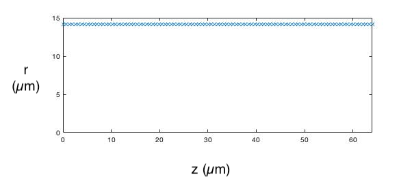
Figure 6: Interface tether position at $t=1$ ms.

Even though the fluid domain is $\Omega=[-32\mu m,32\mu m]\times[0,2\pi]\times[0\mu m,64\mu m]$, the solution is only computed on the computational domain $\Omega=[0\mu m,32\mu m]\times[0\mu m,64\mu m]$ which is the $\theta=0$ slice of the fluid domain. The initial radius of the tube is $R=14.14$ $\mu$m.

The boundary conditions and initial solutions for the full solution and the Stokes and regular parts are given in Section LABEL:subsec:NScylBC. The parameters for this simulation are shown in Table 3.

Table 3: Parameters used for the spatial convergence study of the IIM-OT for 3D Navier-Stokes flow in axisymmetric cylindrical coordinates.

Parameter	Symbol	Value
Viscosity	$\mu$	0.0175 gm/(cm$\cdot$s)
Density	$\rho$	1.055 gm/cm3
Domain length	$L$	64 $\mu$m
Domain height	$H$	32 $\mu$m
Initial tube radius	$R$	14.14 $\mu$m
Simulation length	$T$	1e-3 s
Number of time steps	$N_{t}$	16
Time step size	$\Delta t$	6.25e-5 s
Tether force constant	$a_{Tether}$	2.5e-2 gm/s2
Elastic force constant	$a_{Elastic}$	2.5e-3 gm/s2
Average inlet velocity	$\bar{w}$	1 cm/s

In order to test the spatial convergence of the method, the solution is computed at various spatial resolutions while the time step size $\Delta t$ is held fixed. The solutions are compared with a $513\times 1025$ high-resolution solutions during the at time $t=1$ ms. The results in Table 4 indicate that the method converges with second-order spatial accuracy for all the fluid variables. Additionally, the position $X$ of the interface $\Gamma$ also converges with second-order accuracy.

Table 4: Spatial convergence results for IIM-OT for Navier-Stokes flow in cylindrical coordinates compared to a high resolution $513\times 1025$ solution taken at time $t=1$ms.

Grid Size		$p$		$w$		$u$		$X$
$N_{r}$	$N_{z}$	$||\cdot||_{\infty}$	Order	$||\cdot||_{\infty}$	Order	$||\cdot||_{\infty}$	Order	$||\cdot||_{\infty}$	Order
		1.0e-05 $\times$						1.0e-03 $\times$
33	65	0.1929		0.3530		0.1358		0.3365
65	129	0.0259	2.90	0.0410	3.11	0.0349	1.96	0.0365	3.20
129	257	0.0064	2.02	0.0110	1.90	0.0131	1.41	0.0085	2.10
257	513	0.0008	3.00	0.0026	2.08	0.0028	2.23	0.0016	2.41

4.2.3 Temporal convergence study: moving tethers

In order to test temporal convergence, a series of simulations are run in which an initially a straight tube is actively moved by displacing the time-dependent tether anchors. This test also shows the ability of the method to sharply capture the discontinuities of the fluid solutions and the movement of an active tube. Although, the fluid domain is $\Omega=[0{\rm\mu m},32{\rm\mu m}]\times[0,2\pi]\times[0{\rm\mu m},64{\rm\mu m}]$, the solution is only computed on the computational domain $\Omega=[0{\rm\mu m},32{\rm\mu m}]\times[0{\rm\mu m},64{\rm\mu m}]$ which is the $\theta=0$ slice of the fluid domain. $R=14.1$ $\mu$m is the initial radius of the tube.

The $r$-position of the tethers at position $z$ at time $t$ for the interface is given by

$$R_{tether}(z,t)=R\left(1-\alpha\sin\left(\frac{\pi t}{\beta}\right)\sin\left(\frac{2\pi z}{L}\right)\right)$$ (99)

where $R$ is the initial interface radius, the period is $\beta=.2$ s and the amplitude is $\alpha=0.1$ $\mu$m. The positions of the $N_{b}=100$ interface tethers anchors at $t=0.1$ s are shown in Fig. 7. The boundary conditions and initial solution are given in Section LABEL:subsec:NScylBC. The parameter values for this simulation are given in Table 5.

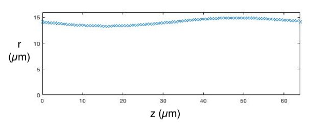
Figure 7: Interface tether anchor position at $t=0.1$ s.

Table 5: Parameters used for the temporal convergence study of the IIM-OT for 3D Navier-Stokes flow in axisymmetric cylindrical coordinates

Parameter	Symbol	Value
Viscosity	$\mu$	.0175 gm/(cm$\cdot$s)
Density	$\rho$	1.055 gm/cm3
Domain length	$L$	64 $\mu$m
Domain height	$H$	32 $\mu$m
Initial tube radius	$R$	14.1 $\mu$m
Simulation length	$T$	.1 s
Grid points in z	$N_{z}$	257
Grid points in r	$N_{r}$	129
Interface control points	$N_{b}$	100
Tether force strength	$a_{\rm tether}$	2.5e-4 gm/s2
Elastic force strength	$a_{\rm elastic}$	2.5e-4 gm/s2
Average inlet velocity	$\bar{w}$	10 $\mu$m/s

In order to determine the temporal accuracy, the solution was computed with various sized time steps while the spatial resolution remained fixed. The solutions were then compared to a high-resolution solution computed with $N_{t}=512$ time steps with a step size of $\Delta t=.0002$ s. The results for this study are given in Table 6. This simulation indicates that the method converges with second-order temporal accuracy for velocity and interface position and near second-order temporal accuracy for pressure.

Table 6: Temporal convergence results for IIM-OT for 3D Navier-Stokes flow in axisymmetric cylindrical coordinates.

Time Step		$p$		$w$		$u$		$X$
$N_{t}$	$\Delta t$	$||\cdot||_{\infty}$	Order	$||\cdot||_{\infty}$	Order	$||\cdot||_{\infty}$	Order	$||\cdot||_{\infty}$	Order
		1.0e-07 $\times$						1.0e-02$\times$
32	.0031	0.7660		0.0147		0.0077		.2925
64	.0016	0.2282	1.75	0.0035	2.07	0.0019	2.02	.0730	2.00
128	.0008	0.0667	1.77	0.0009	1.96	0.0005	1.93	.0177	2.04
256	.0004	0.0287	1.22	0.0002	2.17	0.0001	2.32	.0038	2.21

The interface position at time $t=0.1$s is shown in Fig. 8. The interface is also reflected into the domain $[-H,0]\times[0,L]$ by imposing symmetry over $r=0.$ It can be seen that moving the interface tethers is an effective way to generate interface movement.

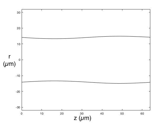
Figure 8: The interface position at time $t=.1$ s. The lower half of the domain is computed by imposing symmetry.

The $w$ component of the velocity and pressure $p$ at times $t=0$s and $t=0.1$s in the computational domain and its reflection over $r=0$ are shown in Figs. 9 and 10, respectively. Note that this method can sharply capture the discontinuities in pressure and the non-smoothness in the velocity. At the time $t=0$ s, the velocity has a parabolic profile, and the pressure is linearly decreasing inside the vessel. At the time $t=0.1$s, the pressure increases at a faster rate where the tube narrows and decreases at a faster rate where the tube widens. The velocity decreases as the tube narrows and increases as the tube widens in the center. Near the distal end of the tube, the velocity decreases again.

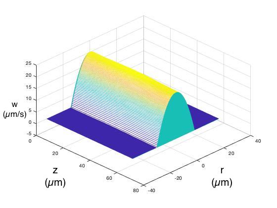
((a)) The $w$ component of velocity at time $t=0$ s exhibits a parabolic profile inside the tube when the interface is straight.

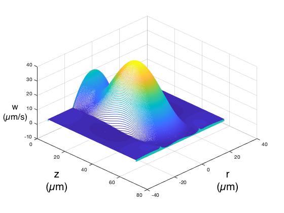
((b)) The $w$ component of velocity at time $t=0.1$ s is greatly affected by the slight change in the interface position caused by the moving tether anchor points.

Figure 9: The $w$ component of velocity at time (a) $t=0$ and at (b) $t=0.1$s are shown in the computational domain and its reflection over $r=0$. The value of $w$ in the lower half of the domain is computed by imposing symmetry.

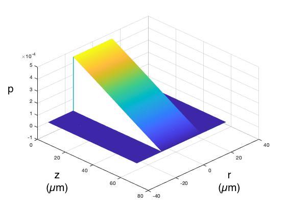
((a)) The pressure $p$ at time $t=0$ in the computational domain is linearly decreasing inside the straight tube.

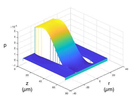
((b)) The pressure $p$ at time $t=0$ in the computational domain is changed by the indentations in the tube walls.

Figure 10: The pressure $p$ at time (a) $t=0$ and at (b) $t=.1$s are shown in the computational domain and its reflection over $r=0$. The value of $p$ in the lower half of the domain is computed by imposing symmetry.

5 Discussion

We have presented a numerical method for simulating viscous fluid flow through an open tube. The model is formulated as an immersed boundary problem, with the channel spanning from one end of the computational domain to the other. We apply the method to the Stokes equations and the Navier Stokes equations. The Stokes equations are solved using a method that is an extension of the immersed interface method, which requires the immersed interface to be closed. This method gives second-order accurate values by incorporating known jumps for the solution and its derivatives into a finite difference method. The Navier-Stokes equations are solved using the velocity decomposition approach. That approach decompose the velocity into a “Stokes” part and a “regular” part. The first part is determined by the Stokes equations and the singular interfacial force. The regular part of the velocity is given by the Navier–Stokes equations with a body force resulting from the Stokes part. The regular velocity is obtained using a time-stepping method that combines the semi-Lagrangian method with the backward difference formula. Numerical examples are presented to demonstrate that, for both the Stokes and Navier-Stokes models, the method converges with second-order spatial and temporal accuracy.

The development of the present method is motivated by our interest in simulating biological problems with flows through biological tubes ^{29, 30, 31, 32, 33, 34, 35, 36, 37, 38, 39, 40, 41, 42, 43, 44, 45, 46, 47} or microfluidic devices.

References

- 1 Patterson SE, Layton AT. Computing Viscous Flow Along a 2D Open Channel Using theImmerse Interface Method. Engineering Report 2021; 3(5): e12334.
- 2 Santhanakrishnan A, Miller LA. Fluid dynamics of heart development. Cell biochemistry and biophysics 2011; 61(1): 1–22.
- 3 Tharakan A, Norton I, Fryer P, Bakalis S. Mass transfer and nutrient absorption in a simulated model of small intestine. Journal of Food Science 2010; 75(6): E339–E346.
- 4 Tang D, Yang C, Walker H, Kobayashi S, Ku DN. Simulating cyclic artery compression using a 3D unsteady model with fluid–structure interactions. Computers & Structures 2002; 80(20-21): 1651–1665.
- 5 Arthurs KM, Moore LC, Peskin CS, Pitman EB, Layton H. Modeling arteriolar flow and mass transport using the immersed boundary method. Journal of Computational Physics 1998; 147(2): 402–440.
- 6 Peskin CS. The immersed boundary method. Acta numerica 2002; 11: 479–517.
- 7 Hou G, Wang J, Layton A. Numerical methods for fluid-structure interaction—a review. Comm Comput Phys 2012; 12: 337–377.
- 8 Peskin CS, McQueen DM. A general method for the computer simulation of biological systems interacting with fluids. In: . 49. London, England: Syndics of the Cambridge University Press,[1947]-2005. ; 1995: 265–276.
- 9 Mittal R, Iaccarino G. Immersed boundary methods. Annu. Rev. Fluid Mech. 2005; 37: 239–261.
- 10 Peskin CS, Printz BF. Improved volume conservation in the computation of flows with immersed elastic boundaries. Journal of computational physics 1993; 105(1): 33–46.
- 11 Mayo A. The fast solution of Poisson’s and the biharmonic equations on irregular regions. SIAM Journal on Numerical Analysis 1984; 21(2): 285–299.
- 12 Leveque RJ, Li Z. The immersed interface method for elliptic equations with discontinuous coefficients and singular sources. SIAM Journal on Numerical Analysis 1994; 31(4): 1019–1044.
- 13 LeVeque RJ, Li Z. Immersed interface methods for Stokes flow with elastic boundaries or surface tension. SIAM Journal on Scientific Computing 1997; 18(3): 709–735.
- 14 Li Z, Lai MC. The immersed interface method for the Navier–Stokes equations with singular forces. Journal of Computational Physics 2001; 171(2): 822–842.
- 15 Lee L, LeVeque RJ. An immersed interface method for incompressible Navier–Stokes equations. SIAM Journal on Scientific Computing 2003; 25(3): 832–856.
- 16 Le DV, Khoo BC, Peraire J. An immersed interface method for viscous incompressible flows involving rigid and flexible boundaries. Journal of Computational Physics 2006; 220(1): 109–138.
- 17 Li Y, Sgouralis I, Layton AT. Computing Viscous Flow in an Elastic Tube.. Numerical Mathematics: Theory, Methods & Applications 2014; 7(4).
- 18 Tan Z, Le DV, Lim KM, Khoo B. An immersed interface method for the incompressible Navier–Stokes equations with discontinuous viscosity across the interface. SIAM Journal on Scientific Computing 2009; 31(3): 1798–1819.
- 19 Xu S, Wang ZJ. An immersed interface method for simulating the interaction of a fluid with moving boundaries. Journal of Computational Physics 2006; 216(2): 454–493.
- 20 Li Y, Williams SA, Layton AT. A hybrid immersed interface method for driven Stokes flow in an elastic tube. Numerical Mathematics: Theory, Methods and Applications 2013; 6(4): 600–616.
- 21 Rosar M, Peskin CS. Fluid flow in collapsible elastic tubes: a three-dimensional numerical model. New York J. Math 2001; 7: 281–302.
- 22 Smith KM, Moore LC, Layton HE. Advective transport of nitric oxide in a mathematical model of the afferent arteriole. American Journal of Physiology-Renal Physiology 2003; 284(5): F1080–F1096.
- 23 Rosar ME. A three-dimensional computer model for fluid flow through a collapsible tube. New York Journal of Mathematics 1994.
- 24 Lai MC, Huang Cy, Huang YM, others . Simulating the axisymmetric interfacial flows with insoluble surfactant by immersed boundary method. Int. J. Numer. Anal. Model 2011; 8(1): 105–117.
- 25 Beale JT, Layton AT. A velocity decomposition approach for moving interfaces in viscous fluids. Journal of Computational Physics 2009; 228(9): 3358–3367.
- 26 Lai MC, Li Z. A remark on jump conditions for the three-dimensional Navier-Stokes equations involving an immersed moving membrane. Applied mathematics letters 2001; 14(2): 149–154.
- 27 Layton A, Spotz W. A semi-Lagrangian double Fourier method for the shallow water equations on the sphere. J Comput Phys 2003; 189: 185–194.
- 28 Xiu D, Karniadakis GE. A semi-Lagrangian high-order method for Navier-Stokes equations. Journal of computational physics 2001; 172(2): 658–684.
- 29 Hu R, McDonough AA, Layton AT. Functional implications of the sex differences in transporter abundance along the rat nephron: modeling and analysis. American Journal of Physiology-Renal Physiology 2019; 317(6): F1462–F1474.
- 30 Layton AT, Edwards A, Vallon V. Renal potassium handling in rats with subtotal nephrectomy: modeling and analysis. American Journal of Physiology-Renal Physiology 2018; 314(4): F643–F657.
- 31 Hu R, McDonough AA, Layton AT. Sex differences in solute transport along the nephrons: effects of Na+ transport inhibition. American Journal of Physiology-Renal Physiology 2020; 319(3): F487–F505.
- 32 Hu R, Layton A. A computational model of kidney function in a patient with diabetes. International Journal of Molecular Sciences 2021; 22(11): 5819.
- 33 Hu R, McDonough AA, Layton AT. Sex differences in solute and water handling in the human kidney: Modeling and functional implications. iScience 2021: 102667.
- 34 Layton AT, Vallon V, Edwards A. Modeling oxygen consumption in the proximal tubule: effects of NHE and SGLT2 inhibition. American Journal of Physiology-Renal Physiology 2015; 308(12): F1343–F1357.
- 35 Layton A, Vallon V, Edwards A. Predicted consequences of diabetes and SGLT inhibition on transport and oxygen consumption along a rat nephron. Am J Physiol Renal Physiol 2016; 310: F1269–F1283.
- 36 Layton AT, Vallon V. SGLT2 inhibition in a kidney with reduced nephron number: modeling and analysis of solute transport and metabolism. American Journal of Physiology-Renal Physiology 2018; 314(5): F969–F984.
- 37 Layton A, Vallon V, Edwards A. A computational model for simulating solute transport and oxygen consumption along the nephrons. Am J Physiol Renal Physiol 2016; 311: F1378–F1390.
- 38 Layton A, Vallon V, Edwards A. Solute transport and oxygen consumption along the nephrons: effects of Na+ transport inhibitors. Am J Physiol Renal Physiol 2016; 311: F1217–F1229.
- 39 Li Q, McDonough AA, Layton HE, Layton AT. Functional implications of sexual dimorphism of transporter patterns along the rat proximal tubule: modeling and analysis. American Journal of Physiology-Renal Physiology 2018; 315(3): F692–F700.
- 40 Edwards A, Castrop H, Laghmani K, Vallon V, Layton A. Effects of NKCC2 isoform regulation on NaCl transport in thick ascending limb and macula densa: a modeling study. Am J Physiol Renal Physiol 2014; 307: F137–F146.
- 41 Layton A, Edwards A, Vallon V. Adaptive changes in GFR, tubular morphology, and transport in subtotal nephrectomized kidneys: modeling and analysis. American Journal of Physiology-Renal Physiology 2017; 313(2): F199–F209.
- 42 Sgouralis I, Evans RG, Layton AT. Renal medullary and urinary oxygen tension during cardiopulmonary bypass in the rat. Mathematical medicine and biology: a journal of the IMA 2017; 34(3): 313–333.
- 43 Sgouralis I, Evans RG, Gardiner BS, Smith JA, Fry BC, Layton AT. Renal hemodynamics, function, and oxygenation during cardiac surgery performed on cardiopulmonary bypass: a modeling study. Physiological reports 2015; 3(1): e12260.
- 44 Chen J, Edwards A, Layton A. Effects of pH and medullary blood flow on oxygen transport and sodium reabsorption in the rat outer medulla. Am J Physiol Renal Physiol 2010; 298: F1369–F1383.
- 45 Chen J, Sgouralis I, Moore LC, Layton HE, Layton AT. A mathematical model of the myogenic response to systolic pressure in the afferent arteriole. American Journal of Physiology-Heart and Circulatory Physiology 2011.
- 46 Fry B, Edwards A, Sgouralis I, Layton A. Impact of renal medullary three-dimensional architecture on oxygen transport. Am J Physiol Renal Physiol 2014; 307: F263–F272.
- 47 Fry BC, Edwards A, Layton AT. Impacts of nitric oxide and superoxide on renal medullary oxygen transport and urine concentration. American Journal of Physiology-Renal Physiology 2015; 308(9): F967–F980.