ABC of the Future

Abstract

Approximate Bayesian computation (ABC) has advanced in two decades from a seminal idea to a practically applicable inference tool for simulator-based statistical models, which are becoming increasingly popular in many research domains. The computational feasibility of ABC for practical applications has been recently boosted by adopting techniques from machine learning to build surrogate models for the approximate likelihood or posterior and by the introduction of a general-purpose software platform with several advanced features, including automated parallelization. Here we demonstrate the strengths of the advances in ABC by going beyond the typical benchmark examples and considering real applications in astronomy, infectious disease epidemiology, personalised cancer therapy and financial prediction. We anticipate that the emerging success of ABC in producing actual added value and quantitative insights in the real world will continue to inspire a plethora of further applications across different fields of science, social science and technology.

keywords — Approximate Bayesian computation, Likelihood-free inference, Simulator-based inference, Bayesian inference

1 Introduction

From its humble beginnings over two decades ago, approximate Bayesian computation, or ABC for short, has more recently been met with ever-increasing excitement and is now regarded as one of the most transformative ideas in the statistical sciences. For in-depth reviews of the history of ABC, its theoretical underpinnings and the most recent developments, see (Marin et al., 2012; Sisson et al., 2018; Beaumont, 2019). In particular, deeper theoretical insights into the large-sample behavior of ABC inference have removed some of the main doubts regarding its statistical validity, and the field is moving rapidly towards a unified understanding of the key aspects that impinge on the asymptotic behavior of ABC approximations. (Fearnhead and Prangle, 2012; Marin et al., 2014; Green et al., 2015; Lintusaari et al., 2017; Frazier et al., 2018; Li and Fearnhead, 2018a, b; Frazier et al., 2020). Nevertheless, the generic application potential of ABC and other likelihood-free inference (LFI) methods has been held back by the computational requirements of its standard inference algorithms and the lack of a suitable all-purpose software implementation. With the advent of more efficient inference strategies adopted from the field of machine learning (Gutmann and Corander, 2016; Gutmann et al., 2018; Lueckmann et al., 2018; Thomas et al., 2021; Kokko et al., 2019; Cranmer et al., 2020; Grazian and Fan, 2019; Papamakarios et al., 2019) and software platforms such as Engine for likelihood-free inference (ELFI) (Lintusaari et al., 2018), ABCpy (Dutta et al., 2017), BSL (An et al., 2019a) and sbi (Tejero-Cantero et al., 2020), to name a few, the immediate prospect of both using and updating the ABC/LFI toolkits for challenging real-world applications certainly looks brighter.

For example, Bayesian optimization for likelihood-free inference (BOLFI), has been shown in several benchmark examples to speed up ABC inference by $3$–$4$ orders of magnitude (Gutmann and Corander, 2016), and multiple successful applications of it beyond typical benchmarks used in the statistical literature have emerged. These include applications in very diverse research fields, such as inverse reinforcement learning for cognitive user interface models (Kangasrääsiö et al., 2017), brain task interleaving modeling (Gebhardt et al., 2020) and more general computational models of cognition (Kangasrääsiö et al., 2019), perturbation modeling and selection in bacterial populations (Corander et al., 2017), direct dark matter detection (Simola et al., 2019), pathogen outbreak modeling (Lintusaari et al., 2019), sound source localisation (Forbes et al., 2021), passenger flow estimation in airports (Ebert et al., 2021), and the modeling of the genetic components that control the transmissibility of pathogens (Shen et al., 2019). To inspire further methodological development, software engineering and dissemination of ABC and other LFI methods, we present here an array of real applications and discuss both the benefits and challenges that lie ahead for this exciting subfield of statistics.

2 Statistical Methodology

2.1 Preliminaries

We briefly introduce the main concepts and the notation used in the following sections, using the simplest form of ABC algorithm for the purpose of illustration. More detailed description of the methods used in the examples, i.e. approximate Bayesian computation–population Monte Carlo (ABC-PMC) (Beaumont et al., 2009) and BOLFI (Gutmann and Corander, 2016) can be found in the following sections.

Bayesian inference is based on calculating the posterior distribution

$$p(\theta\mid y_{\text{\tiny obs}})\propto p(y_{\text{\tiny obs}}\mid\theta)p(\theta)$$ (1)

of the parameters $\theta$ given the observed data $y_{\text{\tiny obs}}$. The commonly employed methods of conducting inference based on the posterior (e.g. optimization, importance sampling, Markov chain Monte Carlo (MCMC)) all require pointwise evaluation of the likelihood, $p(y_{\text{\tiny obs}}\mid\theta)$, at any $\theta$. ABC provides an inferential framework for situations where the likelihood function is not available, or whose evaluation is too computationally challenging, by replacing likelihood evaluation with simulation of the data–generating process, where the latter task is often still feasible even when the former is not.

The rejection ABC algorithm in Algorithm 1 (Tavaré et al., 1997; Pritchard et al., 1999) is the basic formulation of an ABC method. Assuming that the simulator parameter $\theta\in\mathbb{R}^{p}$ is the target of the statistical inference, the rejection ABC algorithm produces $N$ independent samples from an approximate ABC posterior distribution

$$\pi_{\epsilon}(\theta\mid y_{\text{\tiny obs}})\propto\int{\color[rgb]{0,0,0}p}(y^{\prime}\mid\theta){\color[rgb]{0,0,0}p}(\theta)\mathbb{I}_{A_{\epsilon,y_{\text{\tiny obs}}}}(y^{\prime})\text{d}y^{\prime},$$ (2)

where $y^{\prime}$ is artificial data simulated from the generative model, $\mathbb{I}_{A_{\epsilon,y_{\text{\tiny obs}}}}(\cdot)$ is the indicator function for the set $A_{\epsilon,y_{\text{\tiny obs}}}=\{y^{\prime}\mid d(y_{\text{\tiny obs}},y^{\prime})\leq\epsilon\}$, which is defined via a distance metric $d(\cdot,\cdot)$ and a threshold parameter $\epsilon$.

The ABC posterior as defined by (2) is not conditioning on the data exactly, but on a set of artificial data following the distribution of the generative model that is within a tolerance $\epsilon$ from the observed data, as determined by the difference $d(y_{\text{\tiny obs}},y^{\prime})$ between observed and artificial data. Because the relative volume of $A_{\epsilon,y_{\text{\tiny obs}}}$ becomes vanishingly small when the dimension of the data $y_{\text{\tiny obs}}$ increases, sampling-based algorithms such as rejection ABC reduce the sample space in order to perform adequately. Traditionally, this is done by defining a set of summary statistics $s(\cdot)$. Ideally, the summarising function would be a sufficient statistic, but this is rarely available in problems with intractable likelihoods. In practice, $s(\cdot)$ are chosen according to a number of different principles, aimed to maximize the informativeness of the summaries in some sense (Joyce and Marjoram, 2008; Blum, 2010; Drovandi et al., 2011; Fearnhead and Prangle, 2012; Drovandi et al., 2015; Martin et al., 2019). The core of Algorithm 1 is simple and straightforward to implement in most programming languages.

Algorithm 1 Rejection ABC algorithm for $\theta$

for $i=1,\ldots,N$ do

     $d^{\prime}=\infty$

     while $d^{\prime}>\epsilon$ do

         Sample from the prior, $\theta^{\prime}\sim{\color[rgb]{0,0,0}p}(\theta)$

         Simulate from the generative model, $y^{\prime}\sim{\color[rgb]{0,0,0}p}\left(y\mid\theta^{\prime}\right)$

         Calculate distance, $d^{\prime}=d(s(y_{\text{\tiny obs}}),s(y^{\prime}))$

     end while

     Set $\theta^{(i)}=\theta^{\prime}$

end for

2.2 ABC–PMC algorithm

Although the rejection ABC algorithm is still being used frequently as a comparison method in the ABC and LFI literature, there are few applications where it would not be beneficial to instead take advantage of more sophisticated versions of this basic algorithm (Beaumont et al., 2009; Blum, 2010; Csilléry et al., 2010; Drovandi and Pettitt, 2011; Marin et al., 2012; Moral et al., 2012; Clarté et al., 2020; Rodrigues et al., 2020; Simola et al., 2020). The ABC-PMC approach by Beaumont et al. (2009) is an extension of the rejection ABC algorithm based on importance sampling, and aims to improve the efficiency of the procedure by retrieving a sequence of intermediate distributions. The steps of the method are summarized in Algorithm 2. The first iteration of the ABC–PMC algorithm corresponds to the four steps of the basic rejection ABC algorithm with $\epsilon_{1}$. Starting from the second iteration $t\geq 2$, a particle is sampled with replacement from the set of importance weighted particles at iteration $t-1$, it is moved using e.g. a Gaussian kernel, and accepted or rejected based on $\epsilon_{t}<\epsilon_{t-1}$. The importance weight for particle $J=1,\ldots,N$ at iteration $t$ is

$$W_{t}^{(J)}\propto{\color[rgb]{0,0,0}p}(\theta_{t}^{(J)})/\sum_{K=1}^{N}W_{t-1}^{(K)}\phi\left[\tau_{t-1}^{-1/2}\left(\theta_{t}^{(J)}-\theta_{t-1}^{(K)}\right)\right],$$

where $\phi(\cdot)$ is a multivariate Gaussian kernel with mean 0 and identity covariance, and $\tau_{t-1}$ is twice the (weighted) sample covariance of the particles from iteration $t-1$, as recommended in Beaumont et al. (2009).

Algorithm 2 ABC–PMC algorithm for $\theta$

Set $\epsilon_{1}>\ldots>\epsilon_{T}$

if $t=1$ then

     for $J=1,\ldots,N$ do

         while $d_{1}^{(J)}>\epsilon_{1}$ do

              Propose $\theta^{(J)}\sim{\color[rgb]{0,0,0}p}(\theta)$

              Generate $y^{\prime}\sim{\color[rgb]{0,0,0}p}\left(y\mid\theta^{(J)}\right)$

              Calculate $d_{1}^{(J)}={\color[rgb]{0,0,0}d}(s(y_{\text{\tiny obs}}),s(y^{\prime}))$

         end while

         Set weight $W_{1}^{(J)}=N^{-1}$

     end for

else if $2\leq t\leq T$ then

     Set $\tau_{t}=2\cdot\text{cov}\left(\{\theta_{t-1}^{(J)},W_{t-1}^{(J)}\}_{J=1}^{N}\right)$

     for $J=1,\ldots,N$ do

         while $d_{t}^{(J)}>\epsilon_{t}$ do

              Select $\theta_{t}^{*}$ from $\theta_{t-1}^{(J)}$ with probabilities $\left\{W_{t-1}^{(J)}/\sum_{K=1}^{N}W_{t-1}^{(K)}\right\}_{J=1}^{N}$

              Propose $\theta_{t}^{(J)}\sim N(\theta_{t}^{*},\tau_{t})$

              Generate $y^{\prime}\sim{\color[rgb]{0,0,0}p}\left(y\mid\theta_{t}^{(J)}\right)$

              Calculate $d_{t}^{(J)}={\color[rgb]{0,0,0}d}(s(y_{\text{\tiny obs}}),s(y^{\prime}))$

         end while

         Set weight $W_{t}^{(J)}\propto{\color[rgb]{0,0,0}p}(\theta_{t}^{(J)})/\sum_{K=1}^{N}W_{t-1}^{(K)}\phi\left[\tau_{t-1}^{-1/2}\left(\theta_{t}^{(J)}-\theta_{t-1}^{(K)}\right)\right]$

     end for

end if

As a final remark on the ABC–PMC algorithm, both the total number of iterations $T$ and the series of decreasing tolerances $\epsilon_{1}>\epsilon_{2}>\cdots>\epsilon_{T}$ must be selected in advance by the researcher, which might have an impact on the computational performance of the procedure, as well as on the attainability of a suitably accurate approximation of the exact posterior distribution (Silk et al., 2013; Simola et al., 2020). For this reason, rather than defining in advance the series of decreasing tolerances, other choices are possible. In particular, adaptively selecting the tolerance for some iteration $t$ based on a previously defined quantile of the distances of the accepted particles from the previous iteration $t-1$ improves the efficiency of the algorithm in terms of how many times the forward model is used (Lenormand et al., 2013; Weyant et al., 2013; Ishida et al., 2015; Cisewski-Kehe et al., 2019; Simola et al., 2020). For these reasons also a tuning step is often necessary in order to balance the trade–off between computational efficiency and the reliability of the inferential results.

2.3 BOLFI algorithm

Although potentially orders of magnitude more efficient than the basic rejection ABC algorithm, ABC–PMC is based on the idea of identifying relevant regions of the parameter space by finding proposal distributions such that the corresponding simulated datasets are similar within a tolerance to the observed dataset, according to pre-defined summary statistics. As often only weak information is available in advance about what regions are relevant, this requires a large number of datasets to be simulated through the forward model. Lintusaari et al. (2018) notes, for example, that the number of simulated datasets required in the implementation of a sequential ABC sampler like Algorithm 2 is usually at least of order $10^{6}$. If model simulation itself is heavy, the total computational cost of the sequential algorithm becomes very high.

To reduce the need for a large number of potentially costly model simulations, active learning methods adapt the querying process according to different strategies. BOLFI uses Bayesian optimization (Gutmann and Corander, 2016) to construct iteratively a probabilistic surrogate model for the relationship between parameters $\theta^{\prime}$ and discrepancies $d(\theta^{\prime})={\color[rgb]{0,0,0}d}(s(y^{\prime}),s(y_{\text{\tiny obs}}))$ using the growing evidence set $\mathcal{E}_{t}$, which consists of pairs $\{(\theta_{i},d(\theta_{i}))\}_{i=1}^{t}$. The original formulation of BOLFI uses a Gaussian process (GP) as the surrogate model for the discrepancy function, and new evidence $\{(\theta_{t+1},d(\theta_{t+1}))\}$ is sampled from relevant regions of the parameter space. Relevant regions are determined to be parts of the space where the discrepancy is small. The probabilistic model is defined as $d(\theta)\mid\mathcal{E}_{t}\sim GP(\mu_{t}(\theta),v_{t}(\theta)+\sigma^{2})$, where $GP$ is a Gaussian process with mean and variance functions,

$$\mu_{t}(\theta) =k_{t}(\theta)^{T}K_{t}^{-1}[d(\theta_{1}),\ldots,d(\theta_{t})]^{T}$$ (3)

$$v_{t}(\theta)+\sigma^{2} =k(\theta,\theta)-k_{t}(\theta)^{T}K_{t}^{-1}k_{t}(\theta)+\sigma^{2}.$$ (4)

The vector $k_{t}(\theta)=\begin{bmatrix}k(\theta,\theta_{1}),\ldots,k(\theta,\theta_{t})\end{bmatrix}^{T}$ and matrix $K_{t}=[k(\theta_{i},\theta_{j})]\in\mathbb{R}^{t\times t}$ are defined via covariance functions $k(\theta^{\prime},\theta^{\prime\prime})$.

A common choice for a covariance function is the squared exponential covariance function

$$k(\theta^{\prime},\theta^{\prime\prime}) =\sigma_{f}^{2}\exp\left(\sum_{j=1}^{d}\frac{1}{\lambda_{j}^{2}}(\theta^{\prime}_{j}-\theta^{\prime\prime}_{j})^{2}\right),$$ (5)

where parameters $\theta^{\prime}_{j}$ and $\theta^{\prime\prime}_{j}$ are the $j$th elements of $\theta^{\prime}$ and $\theta^{\prime\prime}$. When fitting a GP to the evidence set, the hyperparameters $\sigma$, $\sigma_{f}$, and $\lambda_{j}$ can be optimized iteratively (Rasmussen and Williams, 2006). In practice, it is not necessary to update the hyperparameters given each additional evidence point; instead, a more efficient strategy is to update them with every $T_{\text{update}}$ additional points, for some specified value for $T_{\text{update}}$.

Finally, from $d(\theta)$ we can retrieve a suitable pointwise approximation to the likelihood function

$$L(\theta)\approx\Phi\left(\frac{h-\mu_{t}(\theta)}{\sqrt{v_{t}(\theta)+\sigma^{2}}}\right),$$ (6)

where $\Phi(\cdot)$ is the Gaussian cumulative density, and $h$ is a threshold parameter which we choose to be the minimum of the mean discrepancy $\mu_{t}(\theta)$, although other choices are reasonable. The discrepancies in the evidence set can be log-transformed for possibly improving the GP-fit as advised in Gutmann and Corander (2016). The rest of the steps of the algorithm remain the same.

In practice, an acquisition function is used to determine the locations of relevant parameter space, and there are several reasonable choices for it. Some are directly based on optimizing the density fitting (Järvenpää et al., 2019) while some are efficient for finding the optimum of the function, such as the lower confidence bound selection criterion (LCBSC) (Srinivas et al., 2010; Brochu et al., 2010). LCBSC is defined as

$$\mathcal{A}_{t}(\theta) =\mu_{t}(\theta)-\sqrt{\eta^{2}_{t}v_{t}(\theta)},$$ (7)

where $\eta^{2}_{t}=2\log\left(t^{\frac{d}{2}+2}\pi^{2}/3\epsilon_{\eta}\right)$ is a coefficient depending on the iteration $t$, the dimension of the parameter space $d$ and the tunable parameter $\epsilon_{\eta}$. The parameter value is obtained by minimizing (7) and varying it randomly to further balance exploration and exploitation of the probabilistic function $d(\theta)$. Our approach is to query the simulator at $\theta_{t}$, where

$$\theta_{t}\sim TN(\hat{\theta}_{t},\sigma^{2}_{\text{acq}},a_{L},a_{U}),$$ (8)

where $TN(\hat{\theta}_{t},\sigma^{2}_{\text{acq}},a_{L},a_{U})$ is a normal distribution truncated to interval $[a_{L},a_{U}]$ with mean $\hat{\theta}_{t}=\arg\min_{\theta}\mathcal{A}_{t}(\theta)$ and tunable variance $\sigma^{2}_{\text{acq}}$. Variance $\sigma^{2}_{\text{acq}}$ control the variation from the LCBSC minimum. The interval $[a_{L},a_{U}]$ is the optimization region for the parameter.

BOLFI can be thought as an extension of either an ABC- or a synthetic likelihood (SL)-type method (Wood, 2010). As an SL-type method, the likelihood surrogate and the prior can be used as a target for an MCMC or a Hamiltonian Monte Carlo (HMC) sampling algorithm to draw an approximate posterior sample of size $N_{\text{sample}}$. A popular HMC sampling algorithm is the no-u-turn sampler (NUTS) (Hoffman and Gelman, 2014) which avoids certain sensitivity issues regarding user-defined parameters which the algorithm sets automatically. In this study we use the BOLFI implementation available in ELFI, and the specific version of it is presented in Algorithm 3.

Algorithm 3 BOLFI

for $t=1,\ldots,N_{\text{init}}$ do

     Generate $\theta_{t}\sim{\color[rgb]{0,0,0}p}(\theta)$,

     Generate $y^{\prime}\sim{\color[rgb]{0,0,0}p}\left(y\mid\theta_{t}\right)$

     Calculate $d_{t}={\color[rgb]{0,0,0}d}(s(y_{\text{\tiny obs}}),s(y^{\prime}))$

end for

Set $\mathcal{E}_{N_{\text{init}}}=\{(\theta_{t},d_{t})\}_{t=1}^{N_{\text{init}}}$

Fit $d(\theta)|\mathcal{E}_{N_{\text{init}}}\sim GP(\mu_{N_{\text{init}}}(\theta),v_{N_{\text{init}}}+\sigma^{2})$

Set k = 0

for $t=N_{\text{init}}+1,\ldots,N_{\mathcal{E}}$ do

     if $t\equiv T_{\text{update}}\pmod{T_{\text{update}}}$ then

         Optimize GP-hyperparameters

     end if

     Calculate $\eta^{2}_{t}=2\log\left(t^{\frac{d}{2}+2}\pi^{2}/3\epsilon_{\eta}\right)$

     Calculate $\hat{\theta}_{t}=\arg\min_{\theta}\mu_{t}(\theta)-\sqrt{\eta^{2}_{t}v_{t}(\theta)}$

      Generate $\theta_{t}\sim TN(\hat{\theta}_{t},\sigma^{2}_{\text{acq}},a_{L},a_{U})$

     Generate $y^{\prime}\sim{\color[rgb]{0,0,0}p}\left(y\mid\theta_{t}\right)$

     Calculate $d_{t}={\color[rgb]{0,0,0}d}(s(y_{\text{\tiny obs}}),s(y^{\prime}))$

     Set $\mathcal{E}_{t}=\mathcal{E}_{t-1}\cup\{(\theta_{t},d_{t})\}$

     Fit $d(\theta)\mid\mathcal{E}_{t}\sim GP(\mu_{t}(\theta),v_{t}+\sigma^{2})$ based on $\mathcal{E}_{t}$

     Set k = k + 1

end for

Define $L(\theta)\approx\Phi\left(\frac{h-\mu_{t}(\theta)}{\sqrt{v_{t}(\theta)+\sigma^{2}}}\right)$

Generate $N_{\text{sample}}$ draws from approximate posterior $\propto L(\theta){\color[rgb]{0,0,0}p}(\theta)$

2.4 Recent progress in method development

The features of rejection ABC, i.e. the distance function, the distance threshold and the summarising statistics are still common in many modern ABC algorithms, even if newer methods have achieved superior performance relative to the original formulation of the method.

The basic rejection ABC uses samples generated from the prior, which can be extremely ineffective depending on the informativeness of the prior. ABC-PMC and ABC-sequential Monte Carlo (ABC-SMC) methods (Toni et al., 2009) improve on rejection ABC by sequentially constructing better proposal distributions. Sequential ABC methods have further been improved upon e.g. by introducing adaptivity to the threshold selection (Simola et al., 2020) and the distance function (Prangle, 2017). Other approaches have been introduced to help with summary statistic design and selection (Fearnhead and Prangle, 2012; Thomas et al., 2021). MCMC procedures can also used to generate samples from the approximate posterior distributions (Marjoram et al., 2003; Marjoram, 2013; Vihola and Franks, 2020), and improving their applicability to high-dimensional problems is an on-going research problem (Rodrigues et al., 2020; Clarté et al., 2020).

Parametric approaches such as SL trade the requirement for a distance function and a threshold for a pointwise approximation of the likelihood by a parametric distribution such as a normal distribution. The moments of the approximating likelihood are, in turn, estimated using simulator draws that are possibly summarised (Wood, 2010; Price et al., 2018). The parametric approximation of the posterior enables the use of a variety of methods to draw a representative sample of the posterior (An et al., 2019b). SL methods have also been extended to high-dimensional parameter spaces (Ong et al., 2018).

Recently, density estimation techniques based on deep neural network architectures have been developed for likelihood-free inference (Grazian and Fan, 2019; Lueckmann et al., 2018; Papamakarios et al., 2019). These approaches are similar to the SL-type methods where the likelihood is approximated with a parametric surrogate, but in the place of the parametric distribution, neural network architectures such as autoregressive flows or emulator networks are used to fit either a surrogate model for the likelihood (local approach) or for the simulator (global approach). Furthermore, these methods have also been combined with active learning approaches to minimize the required number of simulator queries. Lueckmann et al. (2018) proposed to minimize the variance of the posterior surrogate as suggested by Järvenpää et al. (2019) in local inference and to maximize information gain in global inference (Houlsby et al., 2011; Gal et al., 2017; Depeweg et al., 2017).

3 ABC in infectious disease epidemiology with application to Ebola outbreaks

Simulator-based inference is well suited to infectious disease epidemiology. For example, it has been used to resolve the outbreak dynamics of stochastic birth-death-mutation models (Lintusaari et al., 2019), and to infer the transmission dynamics of the Ebola haemorrhagic fever outbreak in 1995 in the Democratic Republic of Congo (McKinley et al., 2009) and the COVID-19 pandemic (Chinazzi et al., 2020). In this case study, we demonstrate the application of simulator models to gain insight into the epidemic caused by the emergence of the Ebola virus in West Africa in 2014 as reported by the WHO Ebola Response Team (Team WER) (WHO Ebola Response Team, 2014) to infer the basic reproduction number $R_{0}$, i.e. the mean value of secondary infections caused by an infectee when no control measures are in place. The computational complexity of the recent, individual-based simulator models can be substantial and the pace at which inference can be delivered is of particular importance to determine the severity of the situation, and the predicted progress under different hypotheses. Therefore, active learning-based methods such as BOLFI in Algorithm 3 provide a strategy to minimize the number of simulator queries and to quickly approximate the posterior for $R_{0}$.

3.1 Team WER model

WHO Ebola Response Team (2014) estimated the basic reproduction number by modeling the incidence of onset $I(\cdot)$ at time $t$ with a Poisson process

$$I(t)\sim\mathsf{Poisson}\left(R_{0}\sum_{s=1}^{T_{\text{exp}}}\omega I(t-s)\right),\quad t=1,\ldots,T_{\text{exp}}$$ (9)

which is defined via the basic reproduction number $R_{0}$, the serial interval parameter $\omega$, which is the time difference between the onset of symptoms of the infector and the infectee, and the incidence history $I(0),\ldots,I(t-1)$. The serial interval parameter $\omega$ was determined heuristically from the contact tracing data. It was approximated as gamma-distributed with mean $15$ and coefficient of variation $0.66$. Finally, the time interval $[0,T_{\text{exp}}]$ is the initial period of exponential growth of infections.

In this case, the likelihood for the observed time series can be written as

$$p(I(1),\ldots,I(T_{\text{exp}})\mid R_{0},\omega)=\prod_{t=1}^{T_{\text{exp}}}\mathsf{P}(I(t)=k\mid R_{0},I(1),\ldots,I(t-1),\omega),$$ (10)

and the posterior distribution can be solved analytically when $R_{0}$ is modeled as gamma-distributed a priori. However, Britton and Tomba (2019) argued that even though this population level model has good predictive power, it would tend to lead to underestimation of $R_{0}$. The main causes of the underestimation in the model are the use of the serial intervals instead of generation times which indicate the time between infections of the infectee and infector, and the handling of the contact tracing when there are multiple possible infectors. Both of these aspects, plus other complex factors in the observation process, are simpler to take into account when using a forward simulator-based modeling approach, such as the one described in the next subsection.

3.2 Description of the simulator

We simulate an outbreak of a virus in a homogeneous and infinite community. The general simulation model follows closely the description in Britton and Tomba (2019). The main difference from the model used by WHO Ebola Response Team (2014), is that the forward simulation program generates the state of each infected individual as described by the diagram in Figure 1 instead of via a population level Poisson-process model. Each infected individual will be in one of four possible states: latent, infectious, recovered or perished. After the initial infection, an individual enters the latent period $t_{\text{lat}}$ of the infection. It is modeled as $t_{\text{lat}}\sim\Gamma(2,5)$, where $\Gamma(\alpha,\beta)$ is a gamma-distribution with shape $\alpha$ and scale $\beta$. The latent period is followed by the infectious period $t_{\text{inf}}\sim\Gamma(1,5)$ in which the transfer of the infection to other individuals is possible. The probability of a new infection after $s$ time units since the initial infection follows the infection rate $R_{0}f_{G}(s)$ defined by $R_{0}$ and the generation time distribution $f_{G}(\cdot)$. The individual survives the infectious period with probability $p_{\text{reco}}=0.3$ after a recovery period of $t_{\text{reco}}\sim\Gamma(4,3)$, or perishes with probability (1-$p_{\text{reco}}$) after a period of $t_{\text{die}}\sim\Gamma(4/9,9)$.

For simplicity, we assume that there is no delay in reporting the infection once symptoms arise, and that all of the cases are reported. Assumptions concerning possible reporting bias could be built into the model in a similar fashion as for the other quantities. The time period between infection and symptoms is defined as the incubation period which is the latent period multiplied by an incubation factor $\gamma\sim\text{Uni}\left(0.8,1.2\right)$.

The simulation always starts with a single infected individual and iterates in steps of $\Delta t=0.2$ days until either $104$ weeks pass or $100,000$ individuals have been infected. During each time step the status of each infected individual is checked, and if the current status is infectious, a new individual is infected with probability $p_{\text{inf}}=\Delta t/\Delta T$, where $\Delta T=\hat{t}_{\text{inf}}/R_{0}$ is the mean time between infections and $\hat{t}_{\text{inf}}$ is the mean duration of infectivity.

Notice that in principle it could be possible to construct a likelihood function in this example. However, as the state of each of the infected individual is modeled separately and the number of infected individuals grows exponentially, the resulting combinatorial complexity very quickly prohibits the construction of the likelihood function outside of very small scale simulations.

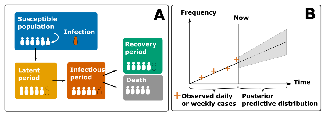
Figure 1: Panel A: In the generative model, each infected subject is in one of the four stages. After the initial infection, the subject is in latent stage and becomes infectious after that. The infectious period ends either in recovery or in death. Panel B: The generative model can be used with the approximate posterior distribution of the basic reproduction number to probabilistically forecast how the infection will spread in the following weeks.

3.3 Inference with BOLFI

The observed data consisted of the daily cumulative count of confirmed cases from the beginning of the $2014$ epidemic for which we infer $R_{0}$. We used the same initial time periods $[0,T_{\text{exp}}]$ for estimating $R_{0}$ as used in WHO Ebola Response Team (2014). The inference was performed separately for Guinea and Liberia using data from March $22$ – March $30$ 2014 and June $16$ – August $20$ 2014, respectively. Subsequent data from the following days were used to illustrate the progression of the virus. In the original study, the authors determined that the initial growth period would be over during the later time period.

The fact that we do not know the true onset of the virus is taken into account by generating artificial counts until we obtain one that exceeds the first observed count, and then continuing the simulation for the same number of days that is in the observed dataset. This way the artificial datasets will have a similar level of variability to the observed one.

The prior for $R_{0}$ is modeled as a truncated normal distribution $TN(1.7,0.5,1.05,4)$. As summary statistic we used the median of slopes of log-transformed case counts that were calculated with consecutive datapoints. As the discrepancy measure ${\color[rgb]{0,0,0}d}(\cdot,\cdot)$ we used the logarithm of the euclidean distance. The BOLFI parameters are listed in Table 1.

To verify $R_{0}$ inference performance, a sample of size $500$ was drawn from the approximate posterior distribution obtained by BOLFI using NUTS sampler. The approximate posterior sample was propagated using the forward simulator, which allows for the investigation of the prediction intervals as a function of time. The propagation of the sample for the following days was visually compared to the actual observed cumulative case count.

BOLFI-parameter	value
$N_{\text{init}}$	5
$N_{\mathcal{E}}$	100
$T_{\text{update}}$	5
$\sigma^{2}_{\text{acq}}$	0.1
$N_{\text{sample}}$	2000

Table 1: BOLFI parameters for the inference of the epidemiological model

3.4 Results using empirical data

The inference results for Guinea and Liberia are illustrated in Figure 2. For Guinea and Liberia, the inferred estimates and $95\%$ credible intervals (CIs) of the basic reproduction number are quite consistent with those reported by WHO Ebola Response Team (2014). For Guinea, they reported an estimate $1.71$ with $95\%$ CI of $1.44$–$2.01$, whereas the BOLFI posterior had a mean of $1.72$ and a $95\%$ CI of $1.19$–$2.33$. For Liberia, Team WER reported an estimate $1.83$ with $95\%$ CI, $1.72$–$1.94$ and BOLFI provided an approximate posterior with mean $1.87$ and $95\%$ CI $1.49$–$2.18$. Reference Althaus (2014) reported maximum likelihood estimates $1.51$ ($95\%$-confidence interval: $1.50-1.52$) and $1.59$ ($95\%$-confidence interval: $1.57-1.60$), for Guinea and Liberia, respectively. The wider uncertainty about $R_{0}$ in our case study CIs reflects the more complex underlying modeling assumptions, and taking such uncertainty appropriately into account may be critical in epidemic management situations.

Forward propagated posterior prediction results consisting of the pointwise median of the simulated trajectories and the $80\%$- and $95\%$-probability bands are also reported in Figure 2 along with the observations used in the inference and some out-of-sample observations that were not used in inference, but are used to illustrate forecasting accuracy. WHO Ebola Response Team (2014) assumed, on a basis of a visual inspection, that the initial period of exponential growth would be $30$ March for Guinea and $24$ August for Liberia which are illustrated with the gray vertical lines on Figure 2. Dates are reported as counts since the beginning of the epidemic (March $22$). Our model fit is consistent with the initial growth period assumption as the observed data counts after the assumed initial growth period diverge quickly from the probable prediction curves.

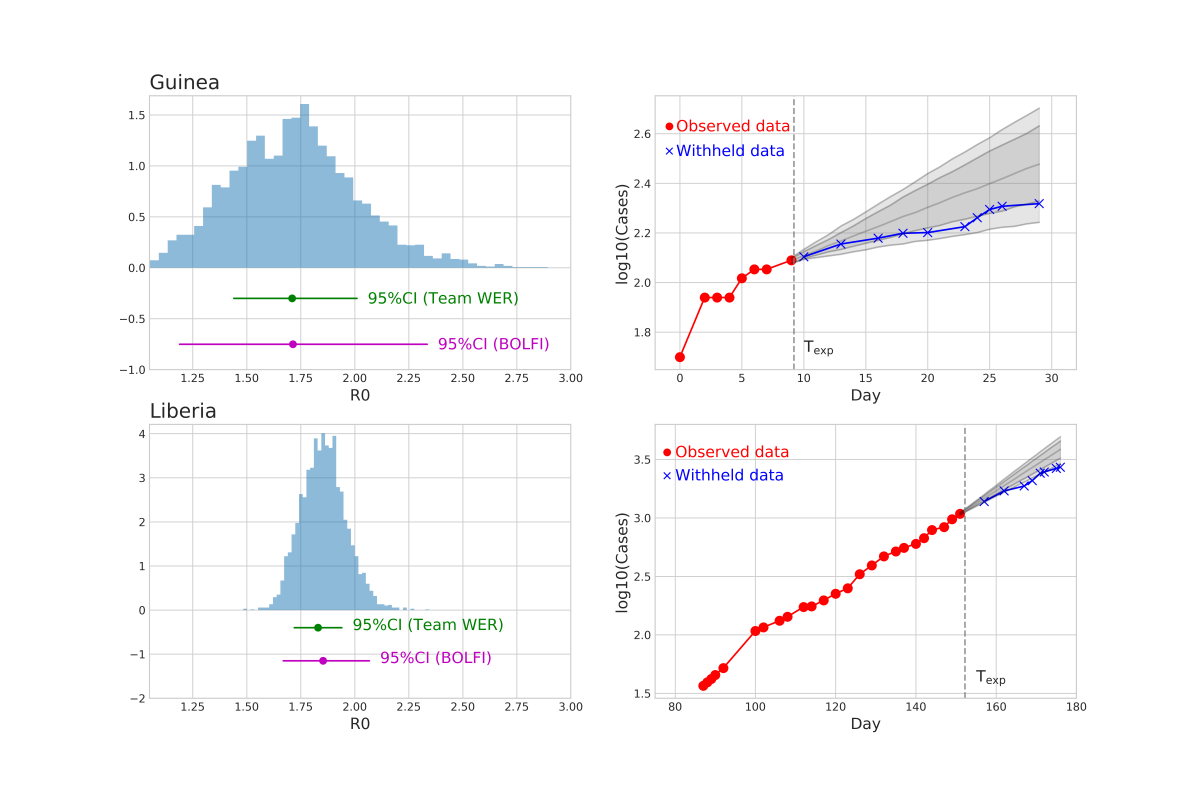
Figure 2: Left: Approximate posterior distributions for $R_{0}$ using data from the initial unconstrained growth period. Results indicate that the subject-level modeling increases the uncertainty about the $R_{0}$ value relative to results reported in WHO Ebola Response Team (2014). Right: The forecast of the number of cumulative infections along with observed data that were used in inference and data withheld from the inference. Ribbons on the plot indicate pointwise $80\%$ and $95\%$ probability intervals of the forecast. Comparison of forecast and withheld data indicates that period of initial growth $T_{\text{exp}}$ as reported in WHO Ebola Response Team (2014) is reasonable.

4 ABC in personalised cancer treatment with application to breast tumor modeling

Personalised cancer treatment is an application area where simulator-based inference has a lot of potential, given the constantly improving biological generative models for the evolution of the disease under treatment (Sottoriva and Tavaré, 2010; Kozłowska et al., 2018; Lai et al., 2019, 2021). Realistic biological generative tumor models that are built up from the molecular and cellular processes result typically in a level of complexity that renders analytical solutions infeasible. Using simulator-based methods we are able to conduct inference on such detailed models, which could in the future be used to optimize personalised treatments to achieve the best possible therapy outcomes. However, the complexity of the biological modeling often makes the generative modeling computationally demanding and only active learning based methods such as BOLFI (Algorithm 3) enable the inference to be performed within a reasonable time.

4.1 Description of the Simulator

We consider an example of breast cancer tumor modeling that is a combination of empirical data and detailed computer simulation. The system is partly initialised and tuned based on a biopsy from a real patient, but we use only simulated data to demonstrate the inference and prediction procedure.

The cancer simulator we use is a multi-scale pharmacokinetic and pharmacodynamic model describing the response of a cross-section of breast tumor tissue to a combination of chemotheraupetic and anti-angiogenic agents (Lai et al., 2019). Mathematically, it consists of a hybrid cellular automaton model (Ribba et al., 2004; Alarcón et al., 2010) that couples stochastic and discrete model formalisms with deterministic and continuous components accounting for biological processes at different spatio-temporal scales; see Figure 3. There are multiple parameters in the model influencing the evolution of cancer cells, stromal cells and tumour vessels, which are all modeled as individual agents. Many of the parameters can be inferred and fixed via various means but some of the unknown parameters have to be inferred based on the reaction of the tumour to the treatment. Here we focus on the inference of two key parameters determining the outcome of each patient to the drug treatment. Those parameters account for the sensitivity of cancer cells to the chemotherapy, $\alpha$, and the minimal cell cycle length of cancer cells, $T_{\text{c}}$. We can write the simulator as a nonlinear time series model for the evolution of state $x_{t}$

$$x_{t}=f_{t}(\alpha,T_{\text{c}},x_{t-1},v_{t}),\quad t=1,2,\ldots,T,$$ (11)

where $f_{t}$ is the nonlinear transition model at $t$, which is the time for the temporally discretized simulator with $30$ minute increments, and $v_{t}$ is the stochastic component of the simulator. The simulated state $x_{t}$ consists of cells, vessels, and extracellular concentrations of oxygen, Avastin and vascular endothelial growth factor (VEGF) within the simulation grid, which here is a $33\times 20$ rectangular grid representing a specific two-dimensional cross-section of the tumor.

The time series model is not available for constant monitoring but some of the components can be indirectly measured at sparse time points using methods such as magnetic resonance imaging. For simplicity we assume that it is possible to measure the true state of the system

$$y_{t_{k}} =x_{t_{k}},\quad k=1,2,\ldots,$$ (12)

In this proof-of-concept study we assume that observations can be collected every three days $t_{k}=k\cdot 3\cdot 48,\leavevmode\nobreak\ k=1,2,\ldots,6$.

The drug is administered for the patient every $3$ weeks, i.e. at times $t^{\text{drug}}_{k}=k\cdot 21\cdot 48,\leavevmode\nobreak\ k=0,1,2,3$ and we aim to infer the parameters within the first $3$-week treatment period, as we would want to forecast whether or not the chosen treatment is effective before the second dose. This dose could be adjusted, given the inferred parameters, to achieve an optimal outcome. Being able to reliably infer the parameters using as little data as possible from the beginning of the cancer evolution curve would enable simulated testing of personalised treatment strategies that are anticipated to be efficient for the specific patient.

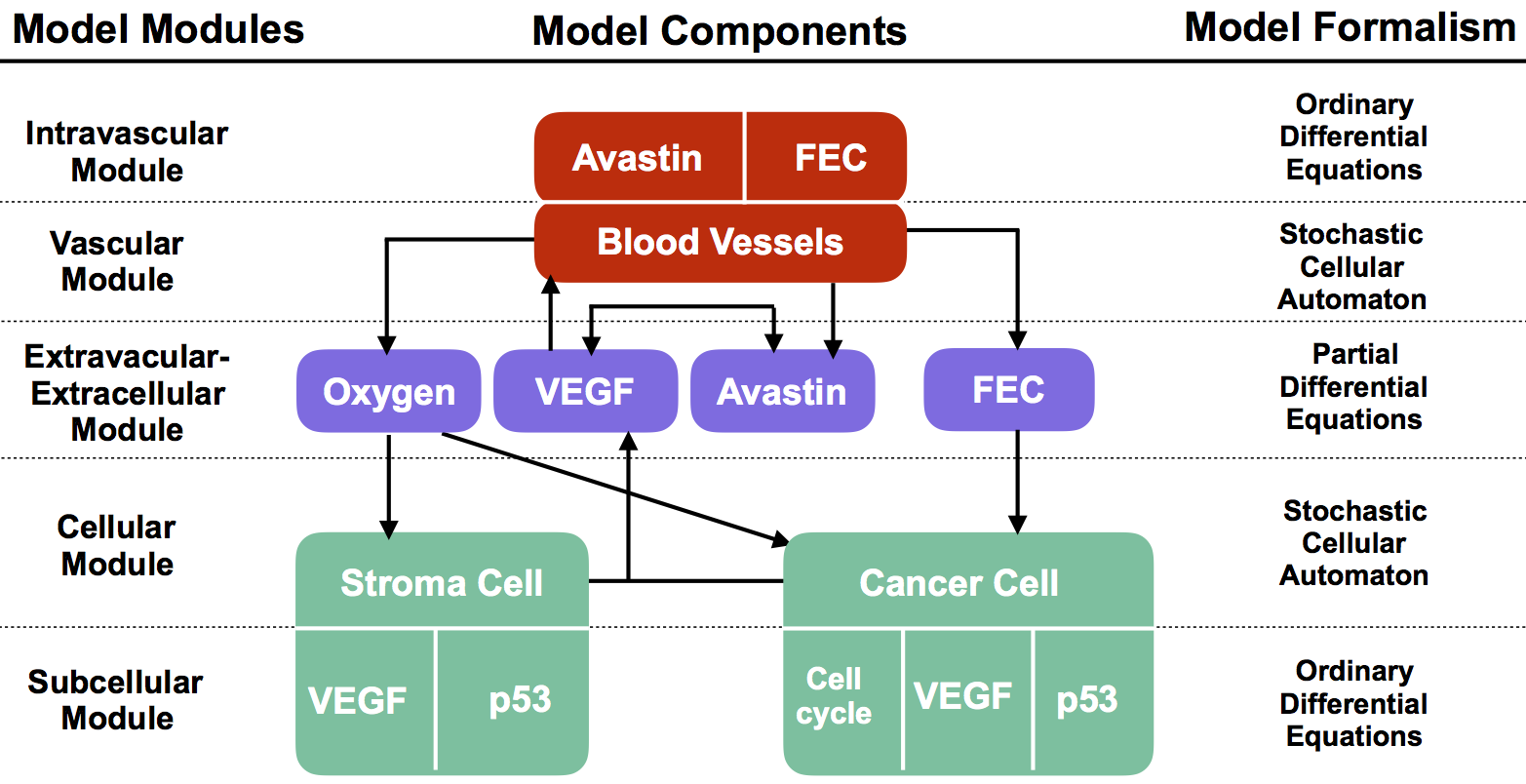
Figure 3: Modular structure of the hybrid cellular automaton describing the response of breast tumor tissue to a cocktail of chemoterapies (FEC) and Avastin. The diagram shows the main components of each module and the interactions among them. The right column shows the different model formalisms used for each of the model modules. See  (Lai et al., 2019) for full model details and its patient-specific parameterisation.

4.2 Inference with BOLFI

We generate the fake observed data using fixed parameter values $T_{\text{c}}=14.69$ and $\alpha=3.0$, and predetermined treatment protocol, and investigate how well we can infer the set parameters and how accurately we are able to forecast the disease progress based on the data collected within the first treatment period. If we were able to infer the patient specific parameter values based on the observed data, then we would be able to forecast how the patient defined by the parameter values would react also to different treatment protocols within the accuracy of the simulator. In our inference framework the results are approximations to the posterior distribution of the parameters $p(\alpha,T_{\text{c}}\mid y_{t_{1}},\ldots y_{t_{6}})$, conditioned on the state observed at $t_{1},\ldots t_{6}$. Prior distributions for the unknown parameters are modelled as uniform $\alpha\sim\text{Uni}\left(1,4\right)$ and $T_{\text{c}}\sim\text{Uni}\left(1,21\right)$

As summary statistics we use the proportions of cancerous cells in the simulation grid at each observation time,

$$s_{k}:=s(y_{t_{k}}) =\frac{1}{660}\sum_{i=1}^{660}y_{t_{k},\text{cells}}^{(i)},\quad k=1,\ldots,6$$ (13)

where $660=33\cdot 20$, is the size of the simulation grid and $y_{t,\text{cells}}^{(i)},i=1,\ldots,660$ is the vectorized simulation grid with binary value $1$ when the $i$th grid location contains a cancer cell. The simulations are computationally very demanding and we use BOLFI to produce the approximation of the posterior. The BOLFI parameters are listed in Table 2. We use the log-transformed euclidean distance for the response of the surrogate model within BOLFI.

BOLFI-parameter	value
$N_{\text{init}}$	30
$N_{\mathcal{E}}$	150
$T_{\text{update}}$	10
$\sigma^{2}_{\text{acq}}$	[0.5, 0.1]
$N_{\text{sample}}$	2000

Table 2: BOLFI parameters for the inference of the breast cancer model

After obtaining an approximate posterior curve based on the likelihood surrogate provided by BOLFI, NUTS is used to draw a sample from it, and the generative model is used to propagate the posterior sample in time under the selected treatment. This results in a simulation-based estimate of the posterior predictive distribution of the state $p(x_{t_{\text{end}}}\mid s_{1},\ldots s_{6})$. Here we use the twelve week mark $t_{\text{end}}=4032$ as the end point. This time interval contains four full treatment periods.

4.3 Results

The inference results are illustrated in Figure 4. We see that the posterior distributions have the probability mass peaks located closely around the true values. Importantly, we are able to use the posterior distributions to probabilistically investigate how the disease will evolve under treatment. In Figure 5 we plot the summarised state of the cancer cells for $12$ week treatment period and compare it to the trajectory simulated given the true parameter values. The results indicate that the forecast is quite consistent given the inferred posterior distributions and that the current treatment most likely will not erase the cancerous growth, and other treatments should be investigated for a better outcome.

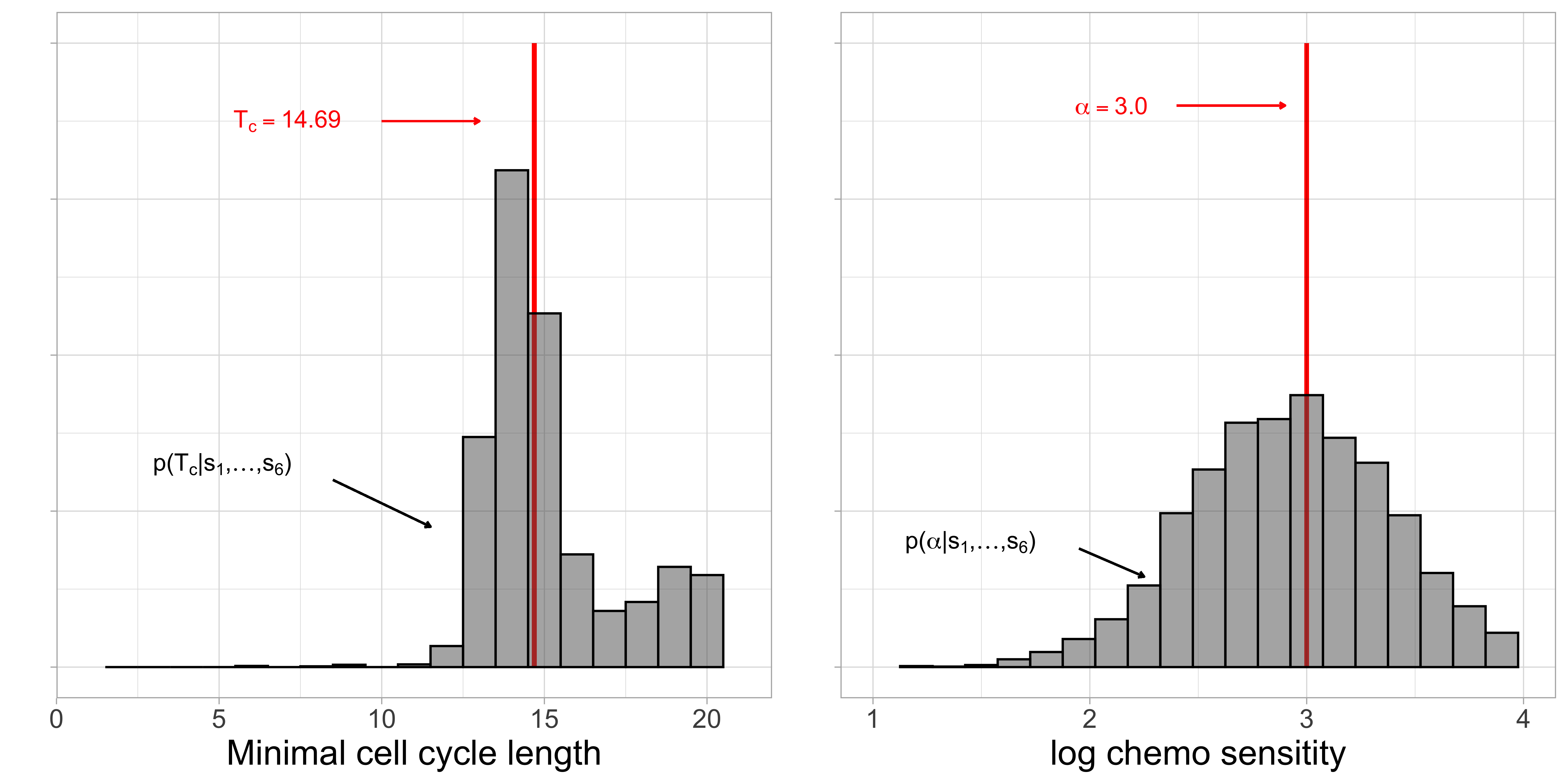
Figure 4: Approximated posterior distributions of the posterior marginals. The red vertical lines on the first two subplots indicate the true simulation values which were used for simulating the cancer cell growth trajectory.

Figure 5: Simulated trajectories of the evolution of cancer cell proportions in the simulation grid given the true parameter values, and the forecast of the trajectory as simulated given the posterior distribution of the parameter values. The simulation end point is highlighted as the histogram on the right.

5 ABC in astronomy with an application to supernova models

Likelihood–free inference is becoming increasingly important in astronomy, where physical models cannot often be fully characterized in terms of a tractable likelihood function (Schafer and Freeman, 2012; Cameron and Pettitt, 2012; Weyant et al., 2013; Ishida et al., 2015; Leclercq, 2018; Picchini et al., 2020). Here we evaluate the performance improvement arising from using BOLFI (Algorithm 3) instead of the ABC–PMC algorithm (introduced in Section 2.2) on an astronomical model from Jennings and Madigan (2017). The ABC–PMC version proposed for this example is slightly different from Algorithm 2. In particular, the version employed for this example requires us to properly tune the final number of iterations $T$, the first tolerance $\epsilon_{1}$ and the quantile $q_{t}$ used for adaptively decreasing the series of tolerances. We did so by following the suggestions in Lenormand et al. (2013) and Weyant et al. (2013). The choices for these three quantities are highlighted in Section 5.1.

Starting with the SuperNova ANAlysis (SNANA) light curve package by Kessler et al. (2009) and the corresponding implementation of the SALT–II light curve fitter presented in Guy et al. (2010), a sample of $400$ supernovae with redshift range $z\in[0.5,1.0]$ have been simulated and then binned into $i=20$ redshift bins. A model that describes the distance modulus as a function of redshift $z$ is defined as:

$$\mu_{i}^{\text{model}}(z_{i};\Omega_{m},w_{0})\propto 5\log_{10}\biggl{(}\frac{c(1+z_{i})}{h_{0}}\biggr{)}\int_{0}^{z_{i}}\frac{dz^{\prime}}{E(z^{\prime})},$$ (14)

where $E(z)=\sqrt{\Omega_{m}(1+z)^{3}+(1-\Omega_{m})\exp\left(3\int_{0}^{z}\text{d}\ln(1+z^{\prime})[1+w(z^{\prime})]\right)}$.

The true cosmological parameters used to generate the “observed” data $\mu$ are the matter density of the universe $\Omega_{m}=0.3$, the dark energy density of the universe $\Omega_{\Lambda}=(1-\Omega_{m})=0.7$, the present value of the dark energy equation $\omega_{0}=-1.0$ and, finally, the current Hubble constant $h_{0}=0.7$. In the following, $\Omega_{\Lambda}$ and $h_{0}$ are considered known and fixed at their input values. The goal is to estimate the two cosmological parameters $\Omega_{m}$ and $\omega_{0}$. The original example as presented in Jennings and Madigan (2017) is available in the astroABC Python package.

Jennings and Madigan (2017) added artificial noise to the data simulated through (14) by using a skew–normal distribution (Azzalini, 1985) with location, scale and skewness parameters fixed at $-0.1$, $0.3$ and $5.0$, respectively. By doing so, the commonly used MCMC algorithm for Bayesian statistical inference is not applicable. In fact, in order the perform the analyses by using the MCMC algorithm, Jennings and Madigan (2017) tried to add artificial noise to the data simulated through Eq. (14) by using a normal distribution with location and scale parameters fixed at $-0.1$ and $0.3$, respectively. The results obtained by the MCMC algorithm (see Section 5 in Jennings and Madigan (2017)) led to a poor estimation of the parameters of interest and therefore an ABC based approach is preferred (Jennings and Madigan, 2017).

The goal of the analysis presented in Jennings and Madigan (2017) was to present a comparison between this slightly more complicated model (for which the ABC–PMC algorithm is required) and a simplified version for which artificial noise is not added (for which the likelihood function is tractable and therefore MCMC is possible). The contour plot of the joint distribution ($\Omega_{m}$, $\omega_{0}$) obtained by using the MCMC algorithm and the marginal posterior means for $\Omega_{m}$ and $\omega_{0}$ are available in Jennings and Madigan (2017). Beyond retrieving reliable summaries such as marginal posterior means and marginal highest posterior density (HPD) intervals for the parameters of interest, it is of relevance from a physics standpoint to evaluate how well a likelihood-free inference approach preserves the so–called “banana–shape” (Kessler et al., 2013; Hinton et al., 2019) that describes the relation between $\Omega_{m}$ and $\omega_{0}$. The “banana–shape” is not expected to significantly change after the artificial noise is added to the data, as shown by Jennings and Madigan (2017).

In order to use BOLFI (introduced in Section 2.3) and the ABC–PMC sampler for the estimation of the matter density of the universe parameter $\Omega_{m}$ and the dark energy equation parameter $\omega_{0}$, two additional quantities must be specified. As highlighted in Section 2, the distance function used to compare the observed and the simulated data and the prior distributions for the parameters of interest (i.e. for this example $\Omega_{m}$ and $\omega_{0}$) must be defined. Since in this section we want to compare the performance of BOLFI with the ABC–PMC sampler, we performed the analysis for both methods by using the same specifications recommended in Jennings and Madigan (2017). The metric ${\color[rgb]{0,0,0}d(\cdot,\cdot)}$ that compares the observed data $\mu$ with the simulated data $\mu_{\text{sim}}(z)$ is defined as:

$${\color[rgb]{0,0,0}d}(\mu,\mu_{\text{sim}}(z))=\sum_{i}\frac{(\mu_{i}-\mu_{\text{sim}}(z_{i}))^{2}}{2\sigma_{i}^{2}},$$ (15)

where $\sigma_{i}$ is the error on the data point $\mu_{i}$, estimated by calculating the sample variance of the observation in the $i^{th}$ bin. We note that, in this example, Jennings and Madigan (2017) do not formally define a summary statistic for the data. Therefore the summary statistic is equivalent to the $20$ dimensional vector of the data. The prior distributions, $\Omega_{m}\sim N(0.3,0.5)$ and $\omega_{0}\sim N(-1.0,0.5)$, are chosen, where the prior for $\Omega_{m}$ is consistent with the $(0,1)$ range for this parameter.

5.1 ABC-PMC inference and acceleration by BOLFI

The ABC–PMC sampler from the astroABC package was run using $N=1000$ particles, a total number of iterations $T=20$ and a quantile equal to $q_{t}=0.75$, which is used to reduce the ABC tolerance parameter through the iterations. It follows that, with respect to the ABC–PMC sampler defined in Algorithm 2, the vector of the ABC tolerances $\epsilon_{1},\dots,\epsilon_{20}$ is not tuned in advance by the researcher but instead defined through the approach suggested by Lenormand et al. (2013), among others. The perturbation kernel used from the second iteration onwards in Algorithm 2 follows the recommended Gaussian distribution, having variance equal to twice the empirical coverage amongst the particles for both $\Omega_{m}$ and $\omega_{0}$. Following the choices by Jennings and Madigan (2017), the first tolerance was fixed to $\epsilon_{1}=500$ and the final tolerance was $\epsilon_{20}=29.82$. We tried different combinations of $T,q_{t}$ in order to identify a suitable level for the final tolerance at which to stop the ABC–PMC algorithm, resulting in $\epsilon_{T}$ close to $30$.

BOLFI-parameter	value
$N_{\text{init}}$	50
$N_{\mathcal{E}}$	300
$T_{\text{update}}$	1
$\sigma^{2}_{\text{acq}}$	1
$N_{\text{sample}}$	1000

Table 3: BOLFI parameters for the estimation of the supernova model

The computational efficiency of both the ABC–PMC sampler and BOLFI was investigated. Our parameter choices for BOLFI are summarized in Table 3. We used a Metropolis-Hasting algorithm to produce the $N_{\text{sample}}$ approximate posterior draws. With the selected particle sample size of $N=1000$, the ABC–PMC sampler takes $90$ minutes to produce the final ABC posterior distribution. In comparison, BOLFI produces the posterior distribution in $3$ minutes. The gain in computational efficiency is a clear advantage obtained by using BOLFI over the ABC–PMC sampler. Figure 6 displays the contour plots of the joint distribution ($\Omega_{m}$, $\omega_{0}$) obtained by the ABC–PMC sampler and by BOLFI, while the point estimates for $\Omega_{m}$ and $\omega_{0}$ obtained by the ABC–PMC analysis (the weighted marginal posterior means) and the estimates retrieved by BOLFI (the marginal posterior means and marginal posterior medians) are summarized in Table 4. It is possible to note that BOLFI provides marginal posterior means closer to the true values ($\Omega_{m}=0.29$ and $\omega_{0}=-1.06$) compared with the corresponding estimates provided by the ABC–PMC ($\Omega_{m}=0.36$ and $\omega_{0}=-1.22$). Both procedures are able to reconstruct the expected “banana–shape”, although the contour plot obtained by BOLFI presents a smaller lower tail compared with the “banana–shape” retrieved by using the ABC–PMC algorithm. This observation is also confirmed by looking at the marginal $90\%$ HPD credible intervals for $\Omega_{m}$ and $\omega_{0}$, reported in parentheses in Table 4. However, repeated experiments would be required to quantify how well the methods based on different approximations actually estimate the posterior distributions.

Figure 6: (left) Contour plot of the joint distribution ($\Omega_{m}$, $\omega_{0}$) obtained by the ABC–PMC sampler and (right) contour plot of the joint distribution ($\Omega_{m}$, $\omega_{0}$) obtained by BOLFI. The true values ($\Omega_{m}=0.3$, $\omega_{0}=1$) are highlighted with a red circle. Relevant regions of the parameter space are inferred and for both methods the marginal posterior means (and for BOLFI also the marginal posterior medians) are highlighted (see also Table 4). The point estimates obtained by BOLFI are closer to the true values for $\Omega_{m}$ and $\omega_{0}$ compared with the corresponding estimates provided by ABC–PMC. The expected “banana–shape” is reconstructed by both methods, although the contour plot obtained by BOLFI presents a smaller lower tail compared with the “banana–shape” retrieved by using the ABC–PMC algorithm.

	True values	ABC–PMC ($90\%$ HPD)	BOLFI mean ($90\%$ HPD)	BOLFI median ($90\%$ HPD)
$\Omega_{m}$	$0.3$	$0.36$ $(0.18,0.54)$	$0.29$ $(0.055,0.48)$	$0.31$ $(0.055,0.48)$
$\omega_{0}$	$-1$	$-1.22$ $(-2.11,-0.62)$	$-1.06$ $(-1.56,-0.61)$	$-0.98$ $(-1.56,-0.61)$

Table 4: Results obtained by using the ABC–PMC sampler and BOLFI. Together with the obtained point estimates of $\Omega_{m}$ and $\omega_{0}$ (the weighted marginal posterior means for the ABC–PMC analyses and the marginal posterior means and marginal posterior medians for BOLFI), the marginal HPD credible intervals $90\%$ are displayed. BOLFI provides point estimates for the parameters that are closer to the true values compared with the corresponding estimates retrieved by the ABC–PMC sampler. HPD credible intervals $90\%$ for $\Omega_{m}$ and $\omega_{0}$ indicate that the probability mass in the “banana–shape” produced by BOLFI is within a more compact region with with a smaller lower tail compared with the “banana–shape” retrieved by using the ABC–PMC algorithm.

6 ABC forecasting with an application to optimal portfolio allocation

Thus far the discussion has centred primarily on the use of ABC as an inferential method, and on improving the performance of more basic versions of ABC via BOLFI. Whilst BOLFI has been used for prediction in two of the three previous illustrations, any comparison with predictions that would have been produced via exact (likelihood-based) Bayesian inference has not been possible, due simply to the fact that the likelihood function is inaccessible (or, at the very least, challenging) in the given examples.

In this section, we step back from the illustration of ABC in situations where it is essential, to an artificial situation in which the exact posterior and, hence, the exact predictive, is available. The aim of the exercise is to illustrate that an ABC-based predictive distribution can be a very accurate approximation of the exact predictive and, hence, yield equally reliable forecasts. This then provides some reassurance that prediction based on an LFI method has value in those cases where it is indeed the only option, such as those illustrated in this paper. We revert here to the simplest form of rejection ABC in order to emphasize that predictive accuracy does not necessarily depend on using an optimal version of the inferential algorithm.

Let $Y_{n+1}$ denote a scalar random variable, observed at time $n+1$, and generated according to $p(y_{n+1}|\theta,y_{\text{\tiny obs}})$, where $y_{\text{\tiny obs}}=[y_{1},y_{2},...,y_{n}]{{}^{T}}.$ The exact Bayesian predictive (or forecast distribution - we use the terms ‘forecast’ and ‘prediction’, and their variants, synonymously) is $p(y_{n+1}|y_{\text{\tiny obs}})=\int p(y_{n+1}|\theta,y_{\text{\tiny obs}})p(\theta|y_{\text{\tiny obs}})\text{d}\theta\mathbf{,}$ where $p(\theta|y_{\text{\tiny obs}})$ is the exact posterior, defined in the usual way, and $y_{n+1}$ denotes a value in the support of $Y_{n+1}$. In cases where $p(y_{\text{\tiny obs}}|\theta)$ and, hence, $p(\theta|y_{\text{\tiny obs}})$, is inaccessible, $p(y_{n+1}|y_{\text{\tiny obs}})$ is also inaccessible, and a natural solution is to define the approximate Bayesian predictive, $g(y_{n+1}|y_{\text{\tiny obs}})=\int_{\Theta}p(y_{n+1}|\theta,y_{\text{\tiny obs}})\pi_{\epsilon}(\theta\mid y_{\text{\tiny obs}})\text{d}\theta\mathbf{,}$ with $g(y_{n+1}|y_{\text{\tiny obs}})$ produced using the ABC posterior in (2), $\pi_{\epsilon}(\theta\mid y_{\text{\tiny obs}})$, which could be accessed using either Algorithm 1 or Algorithm 2. Alternatively, BOLFI (Algorithm 3) could be used to produce an approximate posterior sample, as described in Section 2.3, noting that a notational change would be required to represent this approximate posterior in the expression for $g(y_{n+1}|y_{\text{\tiny obs}})$.

In an extensive exploration, Frazier et al. (2019) demonstrate, both theoretically and in practical situations, that the differences between $g(y_{n+1}|y_{\text{\tiny obs}})$ and $p(y_{n+1}|y_{\text{\tiny obs}})$ can be negligible, despite there sometimes being substantial differences between the approximate and exact posteriors. Moreover, the authors also demonstrate that ABC-based forecasting can produce reliable forecasts in a fraction of the time required for exact methods, owing to the speed with which $\pi_{\epsilon}(\theta\mid y_{\text{\tiny obs}})$ can be constructed, relative to $p(\theta|y_{\text{\tiny obs}})$.

The simplicity and computational speed of ABC-based forecasting is important in the sphere of economics and finance, where the need to predict the actions, and interactions, of large numbers of economic ‘agents’ leads to complex dynamic models that often challenge the MCMC toolkit and exact Bayesian forecasting. To illustrate this novel use of ABC, we document the performance of ABC-based forecasting, relative to exact forecasting, in a particular empirical example: the production of a utility-optimizing financial portfolio. We reiterate that our illustration is based on the simplest version of ABC, as given in Algorithm 1.

6.1 Optimal Portfolio Allocation: the Role of Prediction

At time $n$, an investor chooses to allocate her wealth $W_{n}$ across $m$ possible investment choices, where at time $(n+1)$ the different investment choices yield random returns denoted by $R_{n+1,i}$, $i=1,2,...,m$, with $R_{n+1}=[R_{n+1,1},...,R_{n+1,m}]{{}^{T}}$. For $\Delta_{m}:=\{{\alpha}\in[0,1]^{m}:\sum_{i=1}^{m}\alpha_{i}=1\}$, the individual’s wealth at time $(n+1)$ is given by $W_{n+1}=W_{n}[1+{\alpha}{{}^{T}}R_{n+1}]$. The goal of portfolio analysis is to discern an “optimal” allocation rule ${\alpha}^{\text{opt}}\in\Delta_{m}$ for the portfolio ${\alpha}{{}^{T}}R_{n+1}$.

The portfolio allocation problem exhibits different solutions depending on the definition of “optimality”. A common approach in economics and finance is to find ${\alpha}^{\text{opt}}$ by maximizing expected utility (of wealth) using von Neumann-Morgenstern expected utility (EU) theory (von Neumann and Morgenstern, 1953): For $u(\cdot):[0,\infty)\rightarrow\mathbb{R}$ a utility function, and $\mathbb{E}_{n}(\cdot)$ denoting expectation conditional on information available at time $n$, the optimal allocation rule is

$${\alpha}_{n+1}^{\text{opt}}=\arg\max_{{\alpha}_{n+1}\in\Delta_{m}}\mathbb{E}_{n}[u(W_{n+1})].$$ (16)

For this illustration we consider the canonical risk-averse investor with power utility function, $u(W_{n+1})=\frac{W_{n+1}^{1-\gamma}}{1-\gamma}$, where $\gamma>1$ denotes the risk aversion parameter. Given a model for conditional returns, $p(R_{n+1}|R_{\text{\tiny obs}})$, where $R_{\text{\tiny obs}}=[R_{1},R_{2},...,R_{n}]{{}^{T}}$, the allocation rule that maximizes the expected utility is given by

$${\alpha}_{n+1}^{\text{opt}} =\arg\max_{{\alpha}_{n+1}\in\Delta_{m}}E_{n}\left(u(W_{n+1})\right)=\arg\max_{{\alpha}_{n+1}\in\Delta_{m}}\int u(W_{n+1})p(R_{n+1}|R_{\text{\tiny obs}})\text{d}R_{n+1}.$$ (17)

Given that $p(R_{n+1}|R_{\text{\tiny obs}})$ is typically unavailable in closed-form, we must resort to simulation to compute the integral in (17): if we can obtain $M$ draws from $p(R_{n+1}|R_{\text{\tiny obs}})$, denoted as $R_{n+1}^{(j)}$, $j=1,...,M$, the value of $\mathbf{\alpha}_{n+1}^{\text{opt}}$ can be approximated numerically by solving

$$\hat{{\alpha}}_{n+1}^{\text{opt}}\equiv\arg\max_{{\alpha}_{n+1}\in\Delta_{m}}\sum_{j=1}^{M}u\left(W_{n}\left[1+{\alpha}_{n+1}{{}^{T}}R_{n+1}^{(j)}\right]\right)/M.$$ (18)

The optimally allocated portfolio at time $n+1$ is then given by $W_{n+1}^{\text{opt}}=W_{n}[1+\widehat{{\alpha}}_{n+1}^{\text{opt}^{T}}R_{n+1}^{\text{obs}}]$, with utility, $u(W_{n+1}^{\text{opt}})$, where $R_{n+1}^{\text{obs}}$ denotes the observed value of $R_{n+1}$. Repeating this exercise over an evaluation period yields a series of such utility values, which can be averaged to produce an estimate of $\mathbb{E}_{n}[u(W_{n+1}^{\text{opt}})]$, $\widehat{\mathbb{E}}_{n}[u(W_{n+1}^{\text{opt}})].$ In what follows, we demonstrate that, in this particular representative example, there is negligible difference between the values of $\widehat{\mathbb{E}}_{n}[u(W_{n+1}^{\text{opt}})]$ produced via exact and approximate predictives associated with a given model for $R_{n+1}$.

6.2 Empirical Example

For the illustration we consider a very simple portfolio, $W_{n+1}=W_{n}[1+{\alpha}_{n+1}{{}^{T}}R_{n+1}],$ where $R_{n+1}=[\exp(y_{n+1}),\exp(rf_{n+1})]{{}^{T}}$ and ${\alpha}_{n+1}=[\alpha_{n+1},1-\alpha_{n+1}]{{}^{T}},$ with $y_{n+1}$ the logarithmic return on the S&P500 market portfolio and $rf_{n+1}$ the (known) logarithmic return on a one-month constant maturity US Treasury Bill, over the period $n$ to $(n+1).$ The monthly S&P500 Total Returns index is sourced from the Chicago Board of Options Exchange (CBOE), and captures both capital gains as well as dividend yields. The Treasury Bill is sourced from the Federal Reserve St Louis (FRED) database. The weight $\alpha_{n+1}\in[0,1]$ determines the proportion of wealth allocated to the risky market portfolio, and is to be chosen according to (18). (See, for example, (Billio et al., 2013).) The monthly data extends from June 1986 to June 2018, totaling 384 observations. The first 324 observations are reserved for inference/training and the final 60 observations (five years) used to estimate expected utility.

We produce the 60 one-step-ahead exact and approximate predictive distributions over the evaluation period based on the following stochastic volatility model for $y_{t}$,

$$y_{t} =\mu+\sqrt{V_{t}}\varepsilon_{t}$$ (19)

$$\ln V_{t} =\omega+\rho\ln V_{t-1}+\sigma v_{t},$$ (20)

where $\varepsilon_{t}\overset{\text{i.i.d.}}{\sim}N(0,1)$ and $v_{t}\overset{\text{i.i.d.}}{\sim}N(0,1)$, with $\varepsilon_{t}$ and $v_{t}$ independent for all $t=1,2,...,n.$ The unknowns comprise the static parameter vector, $\theta=[\rho,\sigma,\omega,\mu]{{}^{T}}$, the vector of (in-sample) latent volatilities, ${V}=[V_{1},V_{2},...,V_{n}]{{}^{T}}$, and the unknown $V_{n+1}$ on which $y_{n+1}$ is conditioned. This model is adequate for capturing the behaviour of monthly returns, and allows for a ready application of an exact algorithm, for this comparative exercise.

Expanding windows are used to produce five predictives - one exact and four approximate - for the 60 time points in the evaluation period, with draws of $\theta$ updated only yearly in all cases. Draws from $p(\theta,{V|}y_{\text{\tiny obs}})$, used to estimate the exact predictive, are produced using a particle Metropolis Hastings (PMH) scheme (Andrieu and Doucet, 2010). The four approximate predictives are produced using the auxiliary likelihood-based ABC approach of Martin et al. (2019) to specify the summary statistics in Algorithm 1. Four alternative models from the generalized autoregressive conditionally heteroscedastic (GARCH) family of volatility models are chosen to define the auxiliary likelihood: a GARCH model with normal errors, a GARCH model with Student’s t errors, an asymmetric GARCH with normal errors, and an asymmetric GARCH model with Student’s t errors. We refer the reader to Chapter 9 of Brooks (2014) for a description of these, and related, models; we simply highlight here that such conditionally deterministic volatility models are suitable for an auxiliary likelihood-based version of ABC, given the closed-form nature of their likelihoods. A nearest-neighbour version of rejection ABC is used, with $N=34992$ and a selection probability of $0.86\%$. See Frazier et al. (2018) for an explanation of the rule adopted to determine these values for a given sample size, $n.$

For each predictive, $M=2000$ draws are used to produce an optimal weight, as per (18), the associated optimal portfolio, and its utility. The 60 values of utility are then averaged for a particular predictive method, with five such numbers produced.

Before discussing the resulting (estimated) expected utilities, we present representative exact and approximate predictives in Panels A and B of Figure 7, for two particular months. We label the predictive estimated using PMH as ‘Exact’ and the approximate predictives constructed using each of these four auxiliary models listed above as: ‘ABC1’, ‘ABC2’, ‘ABC3’ and ‘ABC4’, respectively. The plots demonstrate that there is very little to distinguish between the approximate and exact predictive methods, in particular for June 2018. The similarity between the exact and approximate predictives is further borne out in the expected utility calculations. For a fixed risk aversion parameter of $\gamma=4$, the exact approach yields expected utility of $-4.72$, while the four approximate methods yield expected utilities of $-4.69,$ $-4.70,$ $-4.69$ and $-4.69$. Moreover, the computation time required to produce the exact expected utility is ten times larger than the time required to produce the expected utility via the slowest of the approximate methods, and fifteen times greater than the computation time for the fastest approximate method. A comprehensive set of expected utility estimates were produced, for different degrees of risk aversion, with the same negligible difference between exact and approximate results being in evidence.

We close this section by noting that the close match of the exact and approximate predictives is not simply an artifact of the particular predictive model chosen. In Frazier et al. (2019) (cited earlier), comparable numerical results are documented for a range of different models, including for both continuous and discrete data. Moreover, under the required regularity conditions for Bayesian consistency of both the exact and ABC posteriors, the one-step-ahead exact and ABC-based predictives are shown to merge in the sense that, for a large enough sample size, and for models of any fixed dimension, the predictive distributions are identical.

Figure 7: One-step-ahead predictive densities for September 2014 (Panel A) and June 2018 (Panel B): exact (PMH-based) and approximate (ABC-based).

7 Discussion

ABC and similar likelihood-free inference methods are emerging as an important part of the analysis toolbox in various application areas where we are able to simulate realistic data, but the models are too complicated for likelihood-based inference. Here we have demonstrated various aspects of using this approach in challenging real-world applications that go beyond the typical benchmark examples used in the literature.

A particularly interesting combination of inference and generative modeling is the possibility of learning the parameters of a system based on observed data and simulating the performance under various scenarios, treatments or interventions. For example, one of our case studies involved predicting a patient-specific cancer treatment outcome, which could in the future be an important part of treatment planning, especially as the mathematical modeling of disease evolution under treatments is rapidly improving (Kozłowska et al., 2018). A similar application is found in policy planning for epidemics, as the models of infection control are improving, and different ‘what-if’-scenarios can be explored. Such activities have recently been extensively performed across the world during the Covid-19 pandemic and the iteratively improving understanding about the epidemiology of the virus illustrates the need for proper representations of uncertainties in the model components.

As the modeling proficiency increases, we will be faced with even more difficult inference tasks in higher dimensional domains, with computationally heavier simulators and, in some applications, even requirements for carrying out the inference (and prediction) in real-time. These challenges call for further advances from the statistics and computation community on both the inference algorithms and their efficient implementation via user-friendly software.

References

- Alarcón et al. [2010] T. Alarcón, H. M. Byrne, and P. K. Maini. A multiple scale model for tumor growth. Multiscale Modeling Simulation, 3(2):440, 2010. ISSN 1540-3459. doi: 10.1137/040603760.
- Althaus [2014] C. L. Althaus. Estimating the reproduction number of ebola virus (ebov) during the 2014 outbreak in west africa. PLoS currents, 6, 2014.
- An et al. [2019a] Z. An, L. F. South, and C. Drovandi. BSL: An R Package for Efficient Parameter Estimation for Simulation-Based Models via Bayesian Synthetic Likelihood. arXiv preprint 1907.10940, 2019a.
- An et al. [2019b] Z. An, L. F. South, D. J. Nott, and C. C. Drovandi. Accelerating Bayesian synthetic likelihood with the graphical lasso. Journal of Computational and Graphical Statistics, 28(2):471–475, 2019b.
- Andrieu and Doucet [2010] C. Andrieu and A. Doucet. Particle Markov chain Monte Carlo methods. Journal of the Royal Statistical Society, Series B, 72:263–342, 2010.
- Azzalini [1985] A. Azzalini. A class of distributions which includes the normal ones. Scandinavian journal of statistics, pages 171–178, 1985.
- Beaumont [2019] M. A. Beaumont. Approximate Bayesian Computation. Annual Review of Statistics and Its Application, 6(1):379–403, 2019. doi: 10.1146/annurev-statistics-030718-105212.
- Beaumont et al. [2009] M. A. Beaumont, J.-M. Cornuet, J.-M. Marin, and C. P. Robert. Adaptive approximate Bayesian computation. Biometrika, 96(4):983 – 990, 2009.
- Billio et al. [2013] M. Billio, R. Casarin, F. Ravazzola, and H. K. van Dijk. Time-varying combinations of predictive densities using nonlinear filtering. Journal of Econometrics, 177:213–232, 2013.
- Blum [2010] M. Blum. Approximate Bayesian computation: A nonparametric perspective. Journal of American Statistical Association, 105(491):1178 – 1187, 2010.
- Britton and Tomba [2019] T. Britton and G. S. Tomba. Estimation in emerging epidemics: biases and remedies. Journal of the Royal Society, Interface, 16(150):20180670, 2019. doi: 10.1098/rsif.2018.0670.
- Brochu et al. [2010] E. Brochu, V. M. Cora, and N. de Freitas. A tutorial on Bayesian optimization of expensive cost functions, with application to active user modeling and hierarchical reinforcement learning. arXiv preprint arXiv:1012.2599, 2010.
- Brooks [2014] C. Brooks. Introductory Econometrics for Finance. Cambridge University Press, 2014.
- Cameron and Pettitt [2012] E. Cameron and A. N. Pettitt. Approximate bayesian computation for astronomical model analysis: A case study in galaxy demographics and morphological transformation at high redshift. Monthly Notices of the Royal Astronomical Society, 425:44–65, September 2012.
- Chinazzi et al. [2020] M. Chinazzi, J. T. Davis, M. Ajelli, C. Gioannini, M. Litvinova, S. Merler, A. Pastore y Piontti, K. Mu, L. Rossi, K. Sun, C. Viboud, X. Xiong, H. Yu, M. E. Halloran, I. M. Longini, and A. Vespignani. The effect of travel restrictions on the spread of the 2019 novel coronavirus (covid-19) outbreak. Science, 368(6489):395–400, 2020. ISSN 0036-8075. doi: 10.1126/science.aba9757.
- Cisewski-Kehe et al. [2019] J. Cisewski-Kehe, G. Weller, C. Schafer, et al. A preferential attachment model for the stellar initial mass function. Electronic Journal of Statistics, 13(1):1580–1607, 2019.
- Clarté et al. [2020] G. Clarté, C. P. Robert, R. J. Ryder, and J. Stoehr. Componentwise approximate Bayesian computation via Gibbs-like steps. Biometrika, 11 2020. ISSN 0006-3444. doi: 10.1093/biomet/asaa090.
- Corander et al. [2017] J. Corander, C. Fraser, M. U. Gutmann, B. Arnold, W. P. Hanage, S. D. Bentley, M. Lipsitch, and N. J. Croucher. Frequency-dependent selection in vaccine-associated pneumococcal population dynamics. Narure Ecology & Evolution, 1(12):1950–1960, 2017. doi: 10.1038/s41559-017-0337-x.
- Cranmer et al. [2020] K. Cranmer, J. Brehmer, and G. Louppe. The frontier of simulation-based inference. Proceedings of the National Academy of Sciences, 117(48):30055–30062, 2020. ISSN 0027-8424. doi: 10.1073/pnas.1912789117.
- Csilléry et al. [2010] K. Csilléry, M. G. Blum, O. E. Gaggiotti, and O. François. Approximate Bayesian computation (ABC) in practice. Trends in ecology & evolution, 25(7):410 – 418, 2010.
- Depeweg et al. [2017] S. Depeweg, J. M. Hernández-Lobato, F. Doshi-Velez, and S. Udluft. Decomposition of uncertainty in bayesian deep learning for efficient and risk-sensitive learning. arXiv preprint arXiv:1710.07283, 2017.
- Drovandi et al. [2011] C. Drovandi, A. Pettitt, and M. Faddy. Approximate bayesian computation using indirect inference. Journal of the Royal Statistical Society, Series C, 60:1–21, 2011.
- Drovandi et al. [2015] C. Drovandi, A. Pettitt, and A. Lee. Bayesian indirect inference using a parametric auxiliary model. Statistical Science, 30:72–95, 2015.
- Drovandi and Pettitt [2011] C. C. Drovandi and A. N. Pettitt. Estimation of parameters for macroparasite population evolution using approximate bayesian computation. biometrics. Statistics and Computing, 67(1):225–233, 2011.
- Dutta et al. [2017] R. Dutta, M. Schoengens, J.-P. Onnela, and A. Mira. Abcpy: A user-friendly, extensible, and parallel library for approximate bayesian computation. In Proceedings of the Platform for Advanced Scientific Computing Conference, PASC ’17, pages 8:1–8:9, New York, NY, USA, 2017. Association for Computing Machinery, ACM. ISBN 978-1-4503-5062-4. doi: 10.1145/3093172.3093233.
- Ebert et al. [2021] A. Ebert, R. Dutta, K. Mengersen, A. Mira, F. Ruggeri, and P. Wu. Likelihood-free parameter estimation for dynamic queueing networks: Case study of passenger flow in an international airport terminal. Journal of the Royal Statistical Society: Series C (Applied Statistics), 70(3):770–792, 2021. doi: https://doi.org/10.1111/rssc.12487.
- Fearnhead and Prangle [2012] P. Fearnhead and D. Prangle. Constructing summary statistics for approximate bayesian computation: semi-automatic approximate bayesian computation. Journal of the Royal Statistical Society: Series B (Statistical Methodology), 74(3):419–474, 2012. doi: 10.1111/j.1467-9868.2011.01010.x.
- Forbes et al. [2021] F. Forbes, H. D. Nguyen, T. T. Nguyen, and J. Arbel. Approximate Bayesian computation with surrogate posteriors. working paper or preprint, Feb. 2021.
- Frazier et al. [2018] D. T. Frazier, G. M. Martin, C. P. Robert, and J. Rousseau. Asymptotic properties of approximate bayesian computation. Biometrika, 105:593–607, 2018.
- Frazier et al. [2019] D. T. Frazier, W. Maneesoonthorn, G. M. Martin, and B. P. McCabe. Approximate Bayesian forecasting. International Journal of Forecasting, 35(2):521–539, 2019.
- Frazier et al. [2020] D. T. Frazier, C. P. Robert, and J. Rousseau. Model misspecification in approximate Bayesian computation: consequences and diagnostics. Journal of the Royal Statistical Society, Series B, 2020.
- Gal et al. [2017] Y. Gal, R. Islam, and Z. Ghahramani. Deep bayesian active learning with image data. arXiv preprint arXiv:1703.02910, 2017.
- Gebhardt et al. [2020] C. Gebhardt, A. Oulasvirta, and O. Hilliges. Hierarchical reinforcement learning explains task interleaving behavior. Computational Brain & Behavior, 2020.
- Grazian and Fan [2019] C. Grazian and Y. Fan. A review of approximate bayesian computation methods via density estimation: Inference for simulator-models. WIREs Computational Statistics, n/a(n/a):e1486, 2019. doi: 10.1002/wics.1486.
- Green et al. [2015] P. J. Green, K. Łatuszyński, M. Pereyra, and C. P. Robert. Bayesian computation: a summary of the current state, and samples backwards and forwards. Statistics and Computating, pages 835–862, 2015.
- Gutmann and Corander [2016] M. U. Gutmann and J. Corander. Bayesian optimization for likelihood-free inference of simulator-based statistical models. Journal of Machine Learning Research, 2016.
- Gutmann et al. [2018] M. U. Gutmann, R. Dutta, S. Kaski, and J. Corander. Likelihood-free inference via classification. Statistics and Computing, 28(2):411–425, Mar 2018. ISSN 1573-1375. doi: 10.1007/s11222-017-9738-6.
- Guy et al. [2010] J. Guy, M. Sullivan, A. Conley, N. Regnault, P. Astier, C. Balland, S. Basa, R. Carlberg, D. Fouchez, D. Hardin, et al. The supernova legacy survey 3-year sample: Type ia supernovae photometric distances and cosmological constraints. Astronomy & Astrophysics, 523:A7, 2010.
- Hinton et al. [2019] S. R. Hinton, T. Davis, A. G. Kim, D. Brout, C. B. D’Andrea, R. Kessler, J. Lasker, C. Lidman, E. Macaulay, A. Möller, et al. Steve: a hierarchical bayesian model for supernova cosmology. The Astrophysical Journal, 876(1):15, 2019.
- Hoffman and Gelman [2014] M. D. Hoffman and A. Gelman. The no-u-turn sampler: Adaptively setting path lengths in hamiltonian monte carlo. Journal of Machine Learning Research, 15(47):1593–1623, 2014.
- Houlsby et al. [2011] N. Houlsby, F. Huszár, Z. Ghahramani, and M. Lengyel. Bayesian Active Learning for Classification and Preference Learning. arXiv preprint arXiv:1112.5745, 2011.
- Ishida et al. [2015] E. E. O. Ishida, S. D. P. Vitenti, M. Penna-Lima, J. Cisewski, R. S. de Souza, A. M. M. Trindade, E. Cameron, and V. C. Busti. cosmoabc: Likelihood-free inference via population monte carlo approximate bayesian computation. Astronomy and Computing, 13(C), 11 2015. doi: 10.1016/j.ascom.2015.09.001.